Distributed Primal Decomposition for Large-Scale MILPs

Abstract

This paper deals with a distributed Mixed-Integer Linear Programming (MILP) set-up arising in several control applications. Agents of a network aim to minimize the sum of local linear cost functions subject to both individual constraints and a linear coupling constraint involving all the decision variables. A key, challenging feature of the considered set-up is that some components of the decision variables must assume integer values. The addressed MILPs are NP-hard, nonconvex and large-scale. Moreover, several additional challenges arise in a distributed framework due to the coupling constraint, so that feasible solutions with guaranteed suboptimality bounds are of interest. We propose a fully distributed algorithm based on a primal decomposition approach and an appropriate tightening of the coupling constraint. The algorithm is guaranteed to provide feasible solutions in finite time. Moreover, asymptotic and finite-time suboptimality bounds are established for the computed solution. Montecarlo simulations highlight the extremely low suboptimality bounds achieved by the algorithm.

I Introduction

In this paper, we investigate large-scale Mixed-Integer Linear Programs (MILPs) that are to be solved by a network of agents without a central coordinator. The goal is to minimize the sum of objective functions while satisfying individual constraints and a common, non-sparse coupling constraint. We term these MILPs constraint coupled. Due to the mixed-integer decision variable, the large-scale size and the coupling constraint, these problems turn out to be extremely challenging in a distributed context. This typically arise in several relevant control applications, such as microgrid control, economic dispatch in power systems, task assignment in cooperative robotics. An interesting scenario arises in distributed Model Predictive Control (MPC), where a large set of nonlinear control systems must cooperatively solve a common control task and their states, outputs and/or inputs are coupled through a coupling constraint. Here, the constraint-coupled structure results directly from the problem formulation, and the integrality constraints stem from the MILP approximation of the original optimal control problem [2]. In cooperative MPC schemes, such a complex optimization problem should be ideally solved at each control iteration (see e.g. [3, 4, 5, 6, 7]). Being these problems NP-hard, it is not computationally affordable to achieve exact optimality, however feasible (suboptimal) solutions are often sufficient to guarantee stability. It is thus of great interest to compute “good-quality” feasible solutions of large-scale MILPs.

Since our paper deals with constraint-coupled optimization, we organize the relevant literature in two parts. First, we review existing methods for convex constraint-coupled problems. In the tutorial paper [8], parallel decomposition techniques are reviewed. A distributed gradient descent method is proposed in [9] to solve smooth resource allocation problems. In [10] a regularized saddle-point algorithm for convex optimization problems over networks is analyzed. In [11, 12] distributed algorithms based on Laplacian-gradient dynamics are used to solve economic dispatch over digraphs. In [13, 14] distributed dual decomposition-based algorithms for constraint-coupled problems are analyzed, while [15] proposes a distributed algorithm based on successive duality steps. Approaches for constraint coupled problems based on augmented Lagrangian methods with consensus schemes are investigated in [16, 17]. Finally, a discussion on approaches for convex constraint-coupled problems can be found in the recent survey paper [18].

Second, we review parallel and distributed algorithms for MILPs. In [19] a Lagrange relaxation approach is applied to demand response control in smart grids. In [20] a heuristic for embedded mixed-integer programming is studied to obtain approximate solutions. A first attempt to obtain a distributed approximate solution for MILPs is [21]. Recently, a distributed algorithm has been investigated in [22] to solve a different class of MILPs with shared decision variable. A pioneering work on fast, master-client parallel algorithms to find approximate solutions of our problem set-up is [23]. In [24], an enhanced version has been proposed to improve the quality of the solution. A distributed implementation of [24] is proposed in [25].

The contributions of this paper are as follows. We first focus on constraint-coupled convex problems and provide a distributed algorithm based on a combined relaxation and primal decomposition approach. Thanks to this first analysis, as second and main contribution of the paper, we then propose a distributed optimization algorithm for the fast computation of feasible solutions to large-scale, constraint-coupled MILPs. Our algorithm builds on the distributed primal decomposition applied to a convex approximation of the target MILP with restricted coupling constraint. For the mixed-integer solution estimate computed by the proposed distributed method, we are able to: (i) establish both asymptotic and finite-time feasibility, and (ii) provide both asymptotic and finite-time suboptimality bounds. Thanks to the primal decomposition reformulation, the proposed restriction of the coupling constraint turns out to be tighter than the state of the art. Through an extensive numerical study on randomly generated MILPs, we show that our approach is able to achieve interestingly low suboptimality gaps.

The paper unfolds as follows. In Section II, we introduce the MILP set-up together with useful preliminaries. In Section III, we propose our distributed algorithm which is analyzed in Section IV. In Section V, a numerical study is presented. All the proofs of the theoretical results are deferred to the appendix.

II Optimization Set-up and Preliminaries

In this section, we introduce the problem set-up together with some preliminaries that act as building blocks for the development of our methodology.

II-A Constraint-Coupled Mixed-Integer Linear Program

Let us consider a network of $N$ agents aiming to solve the optimization problem

$$\begin{split}\min_{x_{1},\ldots,x_{N}}\>&\>\textstyle\sum\limits_{i=1}^{N}c_{i}^{\top}x_{i}\\ \textnormal{subj. to}\>&\>\textstyle\sum\limits_{i=1}^{N}A_{i}x_{i}\leq b\\ &\>x_{i}\in X_{i}^{\textsc{milp}},\hskip 42.67912pti\in\{1,\ldots,N\},\end{split}$$ (1)

where, for all $i\in\{1,\ldots,N\}$, the decision variable $x_{i}$ has $p_{i}+q_{i}$ components and the mixed-integer constraint set is of the form $X_{i}^{\textsc{milp}}=P_{i}\cap({\mathbb{Z}}^{p_{i}}\times^{q_{i}})$, for some nonempty compact polyhedron $P_{i}\subset^{p_{i}+q_{i}}$. The decision variables are intertwined by $S$ linear coupling constraints, described by the matrices $A_{i}\in^{S\times(p_{i}+q_{i})}$ and the vector $b\in^{S}$. We assume that problem (1) is feasible and denote by $(x_{1}^{\star},\ldots,x_{N}^{\star})$ an optimal solution with cost $J^{\textsc{milp}}=\sum_{i=1}^{N}c_{i}^{\top}x_{i}^{\star}$. In many control applications, the number of decision variables is typically much larger than the number of coupling constraints. Therefore, in this paper we let $N\gg S$, leading to large-scale instances of problem (1).

We assume each agent $i$ has a partial knowledge of problem (1), i.e., it knows only its local data $X_{i}^{\textsc{milp}}$, $c_{i}$, $A_{i}$ and $b$. The goal for each agent is to compute its portion $x_{i}^{\star}$ of an optimal solution of (1), by means of neighboring communication and local computation. Agents communicate according to a connected and undirected graph $\mathcal{G}=(\{1,\ldots,N\},\mathcal{E})$, where $\mathcal{E}\subseteq\{1,\ldots,N\}^{2}$ is the set of edges. The set of neighbors of $i$ in $\mathcal{G}$ is $\mathcal{N}_{i}=\left\{j\in\{1,\ldots,N\}\mid(i,j)\in\mathcal{E}\right\}$.

To solve MILP (1), one can employ enumeration schemes, such as branch-and-bound or cutting-plane techniques. However, this would not exploit its separable structure and would result into a computationally intensive algorithm. Therefore, in the next subsection we introduce an approximate version of the problem that preserves its structure while allowing for the application of efficient decomposition techniques.

II-B Linear Programming Approximation of the Target MILP

Following [23, 25, 24, 26], let us consider a modified version of problem (1) where the right-hand side of the coupling constraint is restricted by a vector $\sigma\geq 0$ and each mixed-integer set $X_{i}^{\textsc{milp}}$ is replaced by its convex hull, denoted by $\textnormal{conv}(X_{i}^{\textsc{milp}})$. The following convex problem is obtained

$$\begin{split}\min_{z_{1},\ldots,z_{N}}\>&\>\textstyle\sum\limits_{i=1}^{N}c_{i}^{\top}z_{i}\\ \textnormal{subj. to}\>&\>\textstyle\sum\limits_{i=1}^{N}A_{i}z_{i}\leq b-\sigma\\ &\>z_{i}\in\textnormal{conv}(X_{i}^{\textsc{milp}}),\hskip 19.91684pti\in\{1,\ldots,N\},\end{split}$$ (2)

where $z_{i}\in^{p_{i}+q_{i}}$ for all $i\in\{1,\ldots,N\}$. We introduced $z_{i}$ to clearly distinguish continuous variables from their mixed-integer counterparts in problem (1). When $\sigma=0$, problem (2) is a relaxation of problem (1) and preserves its feasibility. When $\sigma>0$, as done in related approaches [23, 25, 24], feasibility of problem (2) must be also assumed (see Assumption IV.1).

The main point in solving the (convex) problem (2) in place of the (nonconvex) original MILP (1) is to reconstruct a feasible solution of (1) starting from a solution of (2). The restriction $\sigma$ is designed to guarantee that the solution is feasible for the coupling constraint and depends on the specific mixed-integer reconstruction procedure. Due to the feasibility assumption, the larger is $\sigma$, the narrower is the class of problems to which the approach can be applied. Notably, our method is no worse than [23] in terms of needed $\sigma$. In fact, numerical experiments highlight an extremely lower restriction magnitude, which, as a byproduct, results also in much less suboptimality of the computed solution.

Next, we introduce a key result based on the Shapley-Folkman lemma.

Proposition II.1.

Let problem (2) be feasible and let $(\bar{z}_{1},\ldots,\bar{z}_{N})$ be any vertex of its feasible set. Then, there exists an index set $I_{\mathbb{Z}}\subseteq\{1,\ldots,N\}$, with cardinality $|I_{\mathbb{Z}}|\geq N-S$, such that $\bar{z}_{i}\in X_{i}^{\textsc{milp}}$ for all $i\in I_{\mathbb{Z}}$. $\square$

A proof is given in the early reference [26] (see also [23] for a more recent proof). Since Proposition II.1 gives a bound on the number of portions that are not mixed integer, the leading idea is to adapt only these portions while keeping the others intact. The approach will heavily rely on a primal decomposition framework whose foundations are reviewed in the next subsection.

II-C Primal Decomposition Review

Primal decomposition is a powerful tool to recast constraint-coupled convex programs such as (2) into a master-subproblem architecture [27]. The right-hand side vector $b-\sigma$ of the coupling constraint is interpreted as a given (limited) resource to be shared among agents. Thus, local allocation vectors $y_{i}\in^{S}$ for all $i$ are introduced such that $\sum_{i=1}^{N}y_{i}=b-\sigma$. To determine the allocations, a master problem is introduced

$$\begin{split}\min_{y_{1},\ldots,y_{N}}\>&\>\textstyle\sum\limits_{i=1}^{N}p_{i}(y_{i})\\ \textnormal{subj. to}\>&\>\textstyle\sum\limits_{i=1}^{N}y_{i}=b-\sigma\\ &\>y_{i}\in Y_{i},\hskip 34.14322pti\in\{1,\ldots,N\},\end{split}$$ (3)

where, for each $i\in\{1,\ldots,N\}$, $p_{i}:^{S}\rightarrow$ is defined as the optimal cost of the $i$-th (linear programming) subproblem

$$\begin{split}p_{i}(y_{i})=\>\min_{z_{i}}\>&\>c_{i}^{\top}z_{i}\\ \textnormal{subj. to}\>&\>A_{i}z_{i}\leq y_{i}\\ &\>z_{i}\in\textnormal{conv}(X_{i}^{\textsc{milp}}).\end{split}$$ (4)

In problem (3), the constraint $Y_{i}\subseteq^{S}$ is the set of $y_{i}$ for which problem (4) is feasible, i.e., such that there exists $z_{i}\in\textnormal{conv}(X_{i}^{\textsc{milp}})$ satisfying the local allocation constraint $A_{i}z_{i}\leq y_{i}$. The following lemma ([27, Lemma 1]) establishes the equivalence between LP (2) and problems (3)–(4).

Lemma II.2.

Let (2) be feasible. Then, (i) the optimal costs of problems (2) and (3) are equal; (ii) if $(y_{1}^{\star},\ldots,y_{N}^{\star})$ is optimal for (3) and, for all $i$, $z_{i}^{\star}$ is optimal for (4) (with $y_{i}=y_{i}^{\star}$), then $(z_{1}^{\star},\ldots,z_{N}^{\star})$ is an optimal solution of (2). $\square$

Note that, given an optimal allocation $(y_{1}^{\star},\ldots,y_{N}^{\star})$, each node can retrieve its portion of an optimal solution of problem (2) by relying only on its local allocation $y_{i}^{\star}$.

III Distributed Primal Decomposition for MILPs

In this section we propose a novel distributed algorithm to compute a feasible solution of MILP (1). A cornerstone of the proposed strategy is the distributed primal decomposition method to solve the convex problem (2). We first present this scheme. Then, we formally describe our algorithm for MILPs together with its underlying rationale.

III-A Distributed Primal Decomposition for Convex Problems

As already discussed, agents can compute the solution to (2) by independently solving problem (4), provided that an optimal allocation $(y_{1}^{\star},\ldots,y_{N}^{\star})$ is available. To compute such optimal allocation, one can think of applying a projected subgradient method to problem (3). By denoting $p(y)=\sum_{i=1}^{N}p_{i}(y_{i})$ the cost function of problem (3) and by letting $t\geq 0$ be an iteration index, the update reads $y^{t+1}=[y^{t}-\alpha^{t}\nabla p(y^{t})]_{\mathcal{Y}}$, where $\alpha^{t}$ is the step-size and $[\cdot]_{\mathcal{Y}}$ denotes the Euclidean projection onto the feasible set of problem (3). The constraints $y_{i}\in Y_{i}$ in $\mathcal{Y}$ can be handled by resorting to a relaxation approach similar to the one used in [15]. As for the constraint $\sum_{i=1}^{N}y_{i}=b-\sigma$, the projection admits a closed-form solution that reads

$$y_{i}^{t+1}=y_{i}^{t}-\frac{\alpha^{t}}{N}\textstyle\sum\limits_{j=1}^{N}\big{(}\nabla p_{i}(y_{i}^{t})-\nabla p_{j}(y_{j}^{t})\big{)},\hskip 22.76228pt\forall\>i$$ (5)

where $\alpha^{t}$ is the step-size. However, the update (5) requires knowledge of the entire vector $(\nabla p_{1}(y_{1}^{t}),\ldots,\nabla p_{N}(y_{N}^{t}))$ and therefore cannot be performed in a distributed way. We next present an effective approach that bridges this gap.

Each agent $i$ maintains a local allocation estimate $y_{i}^{t}$. At each iteration $t\geq 0$, agents compute $\mu_{i}^{t}$ as a Lagrange multiplier of

$$\begin{split}\min_{z_{i},v_{i}}\hskip 34.14322pt&\>c_{i}^{\top}z_{i}+Mv_{i}\\ \textnormal{subj. to}\hskip 8.5359pt\>\mu_{i}:\>&\>A_{i}z_{i}\leq y_{i}^{t}+v_{i}\mathds{1}\\ &\>z_{i}\in\textnormal{conv}(X_{i}^{\textsc{milp}}),\>\>v_{i}\geq 0,\end{split}$$ (6)

where $M>0$ and $\mathds{1}$ is the vector of ones. Then, each agent $i$ receives $\mu_{j}^{t}$ from its neighbors $j\in\mathcal{N}_{i}$ and updates $y_{i}^{t}$ with

$$y_{i}^{t+1}=y_{i}^{t}+\alpha^{t}\textstyle\sum\limits_{j\in\mathcal{N}_{i}}\big{(}\mu_{i}^{t}-\mu_{j}^{t}\big{)},$$ (7)

where $\alpha^{t}$ is the step-size. Note that problem (6) is a modified version of (4) that is feasible for all $y_{i}$ and that $\nabla p_{i}(y_{i}^{t})=\mu_{i}^{t}$ [28, Section 5.4.4]. It is introduced to take into account the constraints $y_{i}\in Y_{i}$ in (3). Intuitively, update (7) is obtained by making the centralized update (5) match the graph sparsity. As for the step-size in (7), the following standard assumption is made.

Assumption III.1.

The step-size sequence $\{\alpha^{t}\}_{t\geq 0}$, with each $\alpha^{t}\geq 0$, satisfies $\sum_{t=0}^{\infty}\alpha^{t}=\infty$, $\sum_{t=0}^{\infty}\big{(}\alpha^{t}\big{)}^{2}<\infty$. $\square$

Next, we formalize the convergence result properties of the distributed primal decomposition algorithm for convex problems described by (6)–(7).

Proposition III.2.

Let Assumption III.1 hold. Moreover, let problem (2) be feasible and let the local allocation vectors $y_{i}^{0}$ be initialized such that $\sum_{i=1}^{N}y_{i}^{0}=b-\sigma$. Then, for a sufficiently large $M>0$, the distributed algorithm (6)–(7) generates an allocation vector sequence $\{y_{1}^{t},\ldots,y_{N}^{t}\}_{t\geq 0}$ and a primal sequence $\{z_{1}^{t},\ldots,z_{N}^{t}\}_{t\geq 0}$ (solutions of problem (6) for all $t\geq 0$) such that

1. $\sum_{i=1}^{N}y_{i}^{t}=b-\sigma$, for all $t\geq 0$;

2. $\operatornamewithlimits{lim\vphantom{p}}_{t\to\infty}\|y_{i}^{t}-y_{i}^{\star}\|=0$ for all $i\in\{1,\ldots,N\}$, where $(y_{1}^{\star},\ldots,y_{N}^{\star})$ is an optimal solution of (3);

3. every limit point of $\{z_{1}^{t},\ldots,z_{N}^{t}\}_{t\geq 0}$ is an optimal (feasible) solution of problem (2). $\square$

The proof relies on a primal decomposition reinterpretation of the algorithm in [15] and is omitted for space constraints. Operatively, the parameter $M>0$ can be chosen by using an iterative update scheme as proposed in [26].

III-B Distributed Algorithm Description

We are now ready to formally introduce our Distributed Primal Decomposition for MILPs. Each agent $i$ maintains a mixed-integer solution estimate $x_{i}^{t}\in X_{i}^{\textsc{milp}}$ and a local allocation estimate $y_{i}^{t}\in^{S}$. At each iteration $t\geq 0$, the local allocation estimate $y_{i}^{t}$ is updated according to (6)–(7). After $T_{f}>0$ iterations, agents compute a tentative mixed-integer solution $x_{i}^{T_{f}}$, based on the last computed allocation $y_{i}^{T_{f}}$ (cf. (8)). Here the notation $\mathop{\rm lex\text{-}min}$ denotes that $\rho_{i},\xi_{i}$ and $x_{i}$ are minimized in a lexicographic order [18]. In Section III-C, we discuss in more detail the meaning of problem (8) and an operative way to solve it. Algorithm 1 summarizes the steps from the perspective of agent $i$.

Initialization: Set $T_{f}>0$, $y_{i}^{0}$ such that $\sum_{i=1}^{N}y_{i}^{0}=b-\sigma$

Evolution: For $t=0,1,\ldots,T_{f}$ do

    Compute $\mu_{i}^{t}$ as a Lagrange multiplier of (6)

    Receive $\mu_{j}^{t}$ from $j\in\mathcal{N}_{i}$ and update $y_{i}^{t+1}$ with (7)

Return $x_{i}^{T_{f}}$ as optimal solution of

$$\begin{split}\mathop{\rm lex\text{-}min}_{\rho_{i},\xi_{i},x_{i}}\>&\>\rho_{i}\\ \textnormal{subj. to}\>&\>c_{i}^{\top}x_{i}\leq\xi_{i}\\ &\>A_{i}x_{i}\leq y_{i}^{T_{f}}+\rho_{i}\mathds{1}\\ &\>x_{i}\in X_{i}^{\textsc{milp}},\>\>\rho_{i}\geq 0.\end{split}$$ (8)

Algorithm 1 Distributed Primal Decomposition for MILPs

A sensible choice for $y_{i}^{0}$ is $y_{i}^{0}=(b-\sigma)/N$. By Proposition III.2, the local allocation vectors $\{y_{1}^{t},\ldots,y_{N}^{t}\}_{t\geq 0}$ converge asymptotically to an optimal solution $(y_{1}^{\star},\ldots,y_{N}^{\star})$ of problem (3). Moreover, owing to Proposition II.1, the asymptotic solution $z_{i}^{\star}$ of problem (6) is already mixed integer for at least $N-S$ agents. As for the remaining (at most) $S$ agents, a recovery procedure is needed to guarantee that they also have have a mixed-integer solution. This is done via step (8). In order to allow for a premature halt of the algorithm, we let all the agents perform (8). In Section IV, an asymptotic and finite-time analysis of Algorithm 1 is provided.

From an implementation point of view, an explicit description of $\textnormal{conv}(X_{i}^{\textsc{milp}})$ in terms of inequalities might not be available. Nevertheless, agents can still obtain an estimate of $\mu_{i}^{t}$ by locally running a dual subgradient method on (6), which involves the solution of small (local) MILPs without needing $\textnormal{conv}(X_{i}^{\textsc{milp}})$. The main limitation of the algorithm is only due to the local computation capability of each node.

III-C Discussion on Mixed-Integer Solution Recovery

In this subsection, we describe in more detail the approach behind problem (8) and how it allows agents to recover a “good” solution of MILP (1). We first describe the procedure at steady state and then show how we cope with the finite number of iterations $T_{f}$.

Let $(z_{1}^{\star},\ldots,z_{N}^{\star})$ be an optimal solution of the approximate problem (2) and let $(y_{1}^{\star},\ldots,y_{N}^{\star})$ be a corresponding allocation of the master problem (3), computed asymptotically by Algorithm 1. A straight approach to recover a mixed-integer solution would be to solve for all $i$ the optimization problem

$$\begin{split}\min_{x_{i}}\>&\>c_{i}^{\top}x_{i}\\ \textnormal{subj. to}\>&\>A_{i}x_{i}\leq y_{i}^{\star}\\ &\>x_{i}\in X_{i}^{\textsc{milp}}.\end{split}$$ (9)

Problem (9) is a (small) local MILP that is reminiscent of the subproblem (4). Depending on the allocation constraint $A_{i}x_{i}\leq y_{i}^{\star}$, problem (9) may be feasible or not. Figure 1 (left) shows an example with $z_{i}\in{\mathbb{Z}}\times$, in which (9) is feasible.

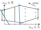
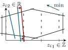
Figure 1: Black lines represent $P_{i}$ while the blue lines are the two components of $A_{i}z_{i}\leq y_{i}^{\star}$. The resulting feasible set is denoted with solid vertical lines. Left: the problem is feasible and admits an optimal solution (red dot), which is mixed integer. Right: the problem is infeasible and the constraint $A_{i}z_{i}\leq y_{i}^{\star}$ is enlarged just enough to include the closest mixed-integer vector (red dot).

In view of Proposition II.1, at least $N-S$ portions $z_{i}^{\star}$ of optimal solution are already mixed-integer and thus optimal for the corresponding local MILPs (9). Recall that $N\gg S$, thus the majority of subproblems (9) are feasible, while the total number of (possibly) infeasible instances is at most $S$. If (9) is infeasible for some agent $i$, we let the agent find a mixed-integer vector with the minimal violation of the allocation constraint as depicted in Figure 1 (right).

The procedure just outlined for the asymptotic case is entirely encoded in problem (8). To see this, let us now show how to operatively solve (8) with $y_{i}^{\star}$ in place of $y_{i}^{T_{f}}$. First, the needed violation of the allocation constraint is determined by computing $\rho^{\infty}_{i}$ as the optimal cost of

$$\begin{split}\min_{\rho_{i},x_{i}}\>&\>\rho_{i}\\ \textnormal{subj. to}\>&\>A_{i}x_{i}\leq y_{i}^{\star}+\rho_{i}\mathds{1}\\ &\>x_{i}\in X_{i}^{\textsc{milp}},\>\>\rho_{i}\geq 0.\end{split}$$ (10)

Then, the value of $\rho_{i}$ is fixed to $\rho^{\infty}_{i}$ and problem (10) is re-optimized with its cost function replaced by $c_{i}^{\top}x_{i}$ to compute $x^{\infty}_{i}$. If problem (9) is feasible, then $\rho^{\infty}_{i}=0$ and the procedure is equivalent to solving (9). Instead, if problem (9) is infeasible, a violation $\rho^{\infty}_{i}\mathds{1}$ of the allocation constraint is permitted.

Due to the violations, the aggregate mixed-integer solution $(x^{\infty}_{1},\ldots,x^{\infty}_{N})$ may exceed the restricted total resource $b-\sigma$. Indeed, although it may not hold $\sum_{i=1}^{N}A_{i}x^{\infty}_{i}\leq b-\sigma$, in the next subsection we show how to design the restriction $\sigma$ to ensure that our original goal $\sum_{i=1}^{N}A_{i}x^{\infty}_{i}\leq b$ is achieved.

Now, let us discuss how this approach can be adapted to cope with the finite number of iterations. The local allocation $y_{i}^{t}$ can be thought of as $y_{i}^{t}=y_{i}^{\star}+\Delta_{i}^{t}$, where $\{\Delta_{i}^{t}\}_{t\geq 0}\to 0$ as $t$ goes to infinity. By looking at problem (10), it is natural to expect that $\rho_{i}^{t}\leq\rho^{\infty}_{i}+\Delta_{i}^{t}$. Thus, we let all the agents perform step (8) (implemented as in the asymptotic case). By employing an additional (small) restriction, we can guarantee that – after a sufficiently large time – the total violation is embedded into the restriction. A detailed analysis of this approach is given in Section IV-B.

III-D Design of the Coupling Constraint Restriction

As already discussed, the purpose of the restriction $\sigma$ is to compensate for possible violations of problem (8). Intuitively, we wish to make $\sigma$ as small as possible for two reasons: the larger is $\sigma$, then (i) the more likely is (2) to be infeasible, (ii) the higher is the cost of the optimal solution $(z_{1}^{\star},\ldots,z_{N}^{\star})$ of (2), which in turn deteriorates the cost of $(x^{\infty}_{1},\ldots,x^{\infty}_{N})$.

We now propose a method to find a small a-priori restriction to guarantee feasibility of the computed solution. As before, we focus on the asymptotic case, while the extension to finite time is given in the following sections. Intuitively, the restriction must take into account the worst-case violation due to the mismatch between $(x^{\infty}_{1},\ldots,x^{\infty}_{N})$ and $(z_{1}^{\star},\ldots,z_{N}^{\star})$. Such worst case occurs when all the (at most $S$) agents for which $z_{i}^{\star}\notin X_{i}^{\textsc{milp}}$ have infeasible instances of (9), leading to a positive violation $\rho^{\infty}_{i}>0$. Thus, we define the a-priori restriction $\sigma^{\infty}\in^{S}$ as

$$\sigma^{\infty}=S\cdot\max_{i\in\{1,\ldots,N\}}\sigma_{i}^{\textsc{loc}},$$ (11)

where $\sigma_{i}^{\textsc{loc}}\in^{S}$ is the worst-case violation of agent $i$ and $\max$ is intended component wise (we stick to this convention from now on).

Let us now quantify $\sigma_{i}^{\textsc{loc}}$. Since $\textnormal{conv}(X_{i}^{\textsc{milp}})$ is bounded, it is possible to find a lower-bound vector, which we denote by $L_{i}\in^{S}$, for any admissible local allocation $y_{i}$,

$$L_{i}\triangleq\!\min_{x_{i}\in\textnormal{conv}(X_{i}^{\textsc{milp}})}A_{i}x_{i}=\!\min_{x_{i}\in X_{i}^{\textsc{milp}}}A_{i}x_{i},$$ (12)

By construction, it holds $L_{i}\leq A_{i}z_{i}^{\star}\leq y_{i}^{\star}$. Recall that each agent computes the needed violation through problem (10). Then, the worst-case violation that may occur at steady-state is $\rho_{i}^{\textsc{max}}\mathds{1}$, where we define $\rho_{i}^{\textsc{max}}$ as

$$\begin{split}\rho_{i}^{\textsc{max}}\triangleq\min_{x_{i}\in X_{i}^{\textsc{milp}}}\>&\>\max_{s\in\{1,\ldots,S\}}\>[A_{i}x_{i}-L_{i}]_{s},\end{split}$$ (13)

where the notation $[\cdot]_{s}$ denotes the $s$-th component of a vector. Note that the optimization in (13) allows each agent $i$ to find the “first” feasible vector, i.e., with minimal resource usage.

In order to reduce possible conservativeness of the violation, which can occur when $\rho_{i}^{\textsc{max}}>\max_{x_{i}\in X_{i}^{\textsc{milp}}}[A_{i}x_{i}-L_{i}]_{s}$ for some component $s$ of the coupling constraint, the computation of $\sigma_{i}^{\textsc{loc}}$ can be replaced by the saturated version

$$\sigma_{i}^{\textsc{loc}}=\min\Big{\{}\rho_{i}^{\textsc{max}}\mathds{1},\>\>\max_{x_{i}\in X_{i}^{\textsc{milp}}}\>(A_{i}x_{i}-L_{i})\Big{\}}.$$

In numerical computations, we have found that usually $\rho_{i}^{\textsc{max}}\ll\max_{x_{i}\in X_{i}^{\textsc{milp}}}\>[A_{i}x_{i}-L_{i}]_{s}$, leading to $\sigma_{i}^{\textsc{loc}}=\rho_{i}^{\textsc{max}}\mathds{1}$.

We point out that the computation of $\sigma^{\infty}$ must be performed in the initialization phase, which can be also carried out in a fully distributed way by using a max-consensus algorithm. In Figure 2, we illustrate an example of the restriction.

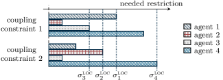
Figure 2: Graphical representation of the restriction for $N=4$ agents and $S=2$ coupling constraints. Each bar represents the quantity $[A_{i}x_{i}-L_{i}]_{s}$ at an optimal solution of (13), which is the violation associated to the first feasible vector with minimal resource usage. The dotted lines represent $\rho_{i}^{\textsc{max}}$ for all $i$, which here coincide with $\sigma_{i}^{\textsc{loc}}$.

Remark III.3.

In [23], an alternative approach based on dual decomposition is explored to compute a feasible solution for MILP (1). The restriction proposed in [23] is

$$\sigma^{\textsc{dd}}=S\cdot\max_{i\in\{1,\ldots,N\}}\>\max_{x_{i}\in X_{i}^{\textsc{milp}}}(A_{i}x_{i}-L_{i}),$$ (14)

The term $\displaystyle\max_{x_{i}\in X_{i}^{\textsc{milp}}}(A_{i}x_{i}-L_{i})$ may be overly conservative and in our approach it is replaced with $\sigma_{i}^{\textsc{loc}}$, which can be thought of as the resource utilization of a feasible vector closest to $L_{i}$. Independently of the problem at hand, it holds $\sigma^{\infty}\leq\sigma^{\textsc{dd}}$. $\square$

IV Analysis of Distributed Algorithm

In this section we provide both asymptotic and finite-time analyses of Algorithm 1 under the following assumption.

Assumption IV.1.

For a given $\sigma\geq 0$, the optimal solution of problem (2) is unique. $\square$

This assumption ensures that the optimal solution of (2) is a vertex (hence Proposition II.1 applies). It can be guaranteed by simply adding a small, random perturbation to the cost vectors $c_{i}$. Notice that Assumption IV.1 is also needed in dual decomposition approaches such as [23, 24, 25]. Notably, dual decomposition approaches require also uniqueness of the dual optimal solution of problem (2), while our approach is less restrictive since this is not necessary.

IV-A Asymptotic analysis

First, we proceed under the assumption that $\sigma=\sigma^{\infty}$ as in (11) and that the algorithm is executed until convergence to an optimal allocation $(y_{1}^{\star},\ldots,y_{N}^{\star})$, i.e., an optimal solution of problem (3). Indeed, steps (6)–(7) implement the distributed algorithm in Section III-A for the solution of problem (2), so that Proposition III.2 (ii) applies.

The next theorem shows feasibility of the computed mixed-integer solution for the target MILP (1).

Theorem IV.2 (Feasibility).

Let $\sigma=\sigma^{\infty}$ as in (11), and let problem (2) be feasible and satisfy Assumption IV.1. Let $(y_{1}^{\star},\ldots,y_{N}^{\star})$ be an optimal solution of problem (3). Then, the vector $(x^{\infty}_{1},\ldots,x^{\infty}_{N})$, with each $x^{\infty}_{i}$ optimal solution of (8) with $y_{i}^{t}=y_{i}^{\star}$, is feasible for MILP (1), i.e., $x^{\infty}_{i}\in X_{i}^{\textsc{milp}}$ for all $i\in\{1,\ldots,N\}$ and $\sum_{i=1}^{N}A_{i}x^{\infty}_{i}\leq b$. $\square$

The proof of Theorem IV.2 is given in appendix.

Remark IV.3.

The proof of Theorem IV.2 reveals that the same result can be obtained by using an allocation $(y_{1},\ldots,y_{N})$ associated to any vertex of the feasible set of problem (2) (rather than an optimal allocation $(y_{1}^{\star},\ldots,y_{N}^{\star})$). Proposition II.1 can still be applied and the proof remains unchanged. $\square$

Theorem IV.2 guarantees that the computed solution is feasible for the target MILP (1), but, in general, there is a certain degree of suboptimality. In the following, we provide suboptimality bounds under Slater’s constraint qualification.

Assumption IV.4.

For a given $\sigma>0$, there exists a vector $(\widehat{z}_{1},\ldots,\widehat{z}_{N})$, with $\widehat{z}_{i}\in\textnormal{conv}(X_{i}^{\textsc{milp}})$ for all $i$, such that

$$\zeta \triangleq\min_{s\in\{1,\ldots,S\}}\Big{[}b-\sigma-\textstyle\sum\limits_{i=1}^{N}A_{i}\widehat{z}_{i}\Big{]}_{s}>0.$$ (15)

The cost of $(\widehat{z}_{1},\ldots,\widehat{z}_{N})$ is denoted by $J^{\textsc{sl}}=\sum_{i=1}^{N}c_{i}^{\top}\widehat{z}_{i}$. $\square$

The following result establishes an a-priori suboptimality bound on the mixed-integer solution with $\sigma=\sigma^{\infty}$ as in (11). Due to space constraints, the proofs of Theorem IV.5 and Corollary IV.6 are omitted. The reader is referred to [23] for similar results.

Theorem IV.5 (A-Priori Suboptimality Bound).

Consider the same assumptions and quantities of Theorem IV.2 and let also Assumption IV.4 hold. Then, $(x^{\infty}_{1},\ldots,x^{\infty}_{N})$ satisfies the suboptimality bound $\sum_{i=1}^{N}c_{i}^{\top}x^{\infty}_{i}-J^{\textsc{milp}}\leq B$, where $J^{\textsc{milp}}$ is the optimal cost of (1) and $B$ is defined as

$$B\triangleq\bigg{(}S+\frac{N\|\sigma^{\infty}\|_{\infty}}{\zeta}\bigg{)}\max_{i\in\{1,\ldots,N\}}\>\gamma_{i},$$

with $\zeta$ defined in (15), and $\displaystyle\gamma_{i}\triangleq\!\!\max_{x_{i}\in X_{i}^{\textsc{milp}}}\!c_{i}^{\top}x_{i}-\!\!\min_{x_{i}\in X_{i}^{\textsc{milp}}}\!c_{i}^{\top}x_{i}$. $\square$

Note that, although the bound provided by Theorem IV.5 is formally analogous to [23, Theorem 3.3], there is an implicit difference due to the restriction values (cf. Remark III.3). In particular, our bound is tighter since $\sigma^{\infty}$ is less than or equal to the restriction proposed by [23].

A tighter bound can be derived by using the steady-state solution of the algorithm and computing also the primal solution of (6) for all $i$. For this reason, we call this bound a posteriori, since it depends on the solution computed by Algorithm 1.

Corollary IV.6 (A-Posteriori Suboptimality Bound).

Consider the same assumptions and quantities of Theorem IV.5. Then, $\sum_{i=1}^{N}c_{i}^{\top}x^{\infty}_{i}-J^{\textsc{milp}}\leq B^{\prime}$, where $B^{\prime}$ is defined as

$$B^{\prime}\triangleq\textstyle\sum\limits_{i\in I_{\mathbb{R}}}(c_{i}^{\top}x^{\infty}_{i}\!-\!c_{i}^{\top}z_{i}^{\star})+\frac{\|\sigma^{\infty}\|_{\infty}}{\zeta}(J^{\textsc{sl}}\!-\!\textstyle\sum\limits_{i=1}^{N}\!c_{i}^{\top}z_{i}^{\star}),$$ (16)

with $\zeta$ and $J^{\textsc{sl}}$ defined in Assumption IV.4 and $I_{\mathbb{R}}$ containing the indices of agents such that $z_{i}^{\star}\notin X_{i}^{\textsc{milp}}$ ($|I_{\mathbb{R}}|\leq S$). $\square$

IV-B Finite-time Analysis

In this section, we provide a finite-time analysis of the distributed algorithm. All the proofs of this subsection are given in appendix. To this end, we assume that the restriction is equal to an enlarged version of the asymptotic restriction in (11), i.e.,

$$\sigma^{\textsc{ft}}=\sigma^{\infty}+\delta\mathds{1},$$ (17)

for an arbitrary $\delta>0$. We assume problem (2) is feasible with this new restriction. We provide two results that extend the results of Section IV-A to a finite-time setting.

At a high level, finite-time feasibility hinges upon the fact that the allocation sequence $\{y_{1}^{t},\ldots,y_{N}^{t}\}_{t\geq 0}$ approaches an optimal allocation. Eventually, the additional restriction $\delta$ can embed the distance of the current allocation estimate to optimality. The next theorem formalizes this result.

Theorem IV.7 (Finite-time feasibility).

Let $\sigma=\sigma^{\textsc{ft}}$ as in (17), for some $\delta>0$, and let problem (2) be feasible and satisfy Assumption IV.1. Consider the mixed-integer sequence $\{x_{1}^{t},\ldots,x_{N}^{t}\}_{t\geq 0}$ generated by Algorithm 1 under Assumption III.1, with $\sum_{i=1}^{N}y_{i}^{0}=b-\sigma^{\textsc{ft}}$. There exists a sufficiently large time $T_{\delta}>0$ such that the vector $(x_{1}^{t},\ldots,x_{N}^{t})$ is a feasible solution for problem (1), i.e., $x_{i}^{t}\in X_{i}^{\textsc{milp}}$ for all $i\in\{1,\ldots,N\}$ and $\sum_{i=1}^{N}A_{i}x_{i}^{t}\leq b$, for all $t\geq T_{\delta}$. $\square$

In principle, the smaller is $\delta$, the longer it takes for the mixed-integer vector $(x_{1}^{t},\ldots,x_{N}^{t})$ to satisfy the coupling constraint. As a function of $\delta$, there is a trade-off between the number of iterations to guarantee solution feasibility and how strict is the assumption that problem (2) is feasible.

Next, we provide a suboptimality bound that can be evaluated when the algorithm is halted.

Theorem IV.8 (Finite-time suboptimality bound).

Consider the same assumptions and quantities of Theorem IV.7 and let also Assumption IV.4 hold. Moreover, let $\epsilon_{i}>0$ for $i\in\{1,\ldots,N\}$. Then, there exists a time $T_{\epsilon}>0$ such that the vector $(x_{1}^{t},\ldots,x_{N}^{t})$ satisfies the suboptimality bound $\sum_{i=1}^{N}c_{i}^{\top}x_{i}^{t}-J^{\textsc{milp}}\leq B^{t}$ for all $t\geq T_{\epsilon}$, with $B^{t}$ being

$$B^{t}\triangleq\textstyle\sum\limits_{i=1}^{N}(c_{i}^{\top}x_{i}^{t}-J_{i}^{\textsc{lp},t})+\textstyle\sum\limits_{i=1}^{N}\epsilon_{i}\|\mu_{i}^{t}\|_{1}+\Gamma\|\sigma^{\textsc{ft}}\|_{\infty},$$ (18)

where $J^{\textsc{milp}}$ is the optimal cost of (1), $J_{i}^{\textsc{lp},t}$ and $\mu_{i}^{t}$ are the optimal cost and a Lagrange multiplier of (6) at time $t$, $\Gamma=\frac{N}{\zeta}\textstyle\sum\limits_{i=1}^{N}\Big{(}\max\limits_{x_{i}\in X_{i}^{\textsc{milp}}}c_{i}^{\top}x_{i}-\min\limits_{x_{i}\in X_{i}^{\textsc{milp}}}c_{i}^{\top}x_{i}\Big{)}$, and $\zeta$ associated to any Slater point (cf. Assumption IV.4). $\square$

We point out that, differently from the asymptotic case, the bound (18) does not depend on the solution of (6), but only on its optimal cost. Moreover, notice that the bound (18) is a posteriori, while if an a-priori bound with restriction $\sigma^{\textsc{ft}}$ is desired, it still has the form of Theorem IV.5 (since it does not depend on the algorithmic evolution).

V Monte Carlo Numerical Computations

In this section, we provide a computational study on randomly generated MILPs to compare Algorithm 1 with [23]. The distributed algorithms are emulated using a single machine with the Matlab software and the local MILPs are solved using the integrated numerical solver.

We consider large-scale problems with a total of $4500$ optimization variables ($3000$ are integer and $1500$ are continuous). There are $N=300$ agents and $S=5$ coupling constraints. The local constraints $X_{i}^{\textsc{milp}}$ are subsets of ${\mathbb{Z}}^{10}\times^{5}$ satisfying $D_{i}x_{i}\leq d_{i}$, where $D_{i}$ and $d_{i}\in^{20}$ have random entries in $[0,1]$ and $[20,40]$ respectively. Box constraints $-60\,\mathds{1}\leq x_{i}\leq 60\,\mathds{1}$ are added to ensure compactness. The cost vector is $c_{i}=D_{i}^{\top}\hat{c}_{i}$, where $\hat{c}_{i}$ has random entries in $[0,5]$. As for the coupling, the matrices $A_{i}$ are random with entries in $[0,1]$ and the resource vector $b\in^{5}$ is random with values in two different intervals. Specifically, we first pick values in $[-20N,-15N]$, which results in a “loose” $b$, then we pick values in $[-180N,-175N]$, which results in a “tight” $b$.

A total of $100$ MILPs with loose $b$ and $100$ MILPs with tight $b$ are generated. For each problem, we check feasibility of problem (2) for both our method and the method in [23]. Then, both algorithms are executed up to asymptotic convergence to evaluate the mixed-integer solution suboptimality. The results are summarized in Figures 3 and 4, where the restriction size is computed as $\|\sigma\|/\|b\|$ and the suboptimality is computed as $\big{(}\sum_{i=1}^{N}c_{i}^{\top}x^{\infty}_{i}-q^{\star}\big{)}/q^{\star}$, with $q^{\star}$ being the optimal cost of (2). The number of solvable instances is the number of problems for which problem (2) is feasible. For loose $b$, both methods are always applicable. However, our approach provides better solution performance than [23]. For tight resource vectors, our method is still applicable in the 70% of the cases, and provides an average suboptimality of 6.91%, while the approach in [23] cannot be applied due to infeasibility of the approximate problem (2) (caused by the too large needed restrictions). It is worth noting that the generation interval $[-180N,-175N]$ cannot be further tightened. Indeed, for smaller values of $b$, the target MILP (1) becomes infeasible.

Finally, we show the evolution of Algorithm 1 on a single instance over an Erdős-Rényi graph with edge probability $0.2$. Figure 5 shows the value of the coupling constraints along the algorithmic evolution, with $\delta=0.5$ (cf. (17)). Note that feasibility is achieved in finite time (within 400 iterations), confirming Theorem IV.7. In order to detect feasibility, agents can run a consensus-based scheme from time to time to check whether the current solution satisfies the coupling constraints.

	Algorithm 1		[23]
	$b$ loose	$b$ tight	$b$ loose	$b$ tight
# solvable problems	100%	70%	100%	0%
size of restriction	7.4%	0.72%	66.9%	6.63%
suboptimality of solution	0.06%	6.91%	0.7%	N.A.

Figure 3: Montecarlo simulations on random MILPs: performance comparison of Algorithm 1 and of the method in [23]. The second and the third row are averaged over the Monte Carlo runs. See the text for further details.

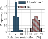
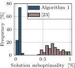
Figure 4: Montecarlo simulations on random MILPs with loose $b$: comparison histograms of Algorithm 1 and of the method in [23]. See the text for details.

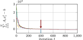
Figure 5: Components of the coupling constraint associated to $(x_{1}^{t},\ldots,x_{N}^{t})$ generated by Algorithm 1 on a random MILP. The agents are assumed to compute the mixed-integer solution according to (8) at each iteration.

VI Conclusions

In this paper we proposed a distributed algorithm to compute a feasible solution to large-scale MILPs with high optimality degree. The method is based on a primal decomposition approach and a suitable restriction of the coupling constraint and guarantees feasibility of the computed mixed-integer vectors in finite time. Asymptotic and finite-time results for feasibility and suboptimality bounds are proved. Numerical simulations highlight the efficacy of the proposed methodology.

Appendix A Proofs

A-A Proof of Theorem IV.2

For the sake of analysis, let us denote by $(z_{1}^{\star},\ldots,z_{N}^{\star})$ the optimal solution of the restricted LP (2). By Assumption IV.1, $(z_{1}^{\star},\ldots,z_{N}^{\star})$ is a vertex, so that by Proposition II.1 there exists $I_{\mathbb{Z}}\subseteq\{1,\ldots,N\}$, with $|I_{\mathbb{Z}}|\geq N-S$, such that $z_{i}^{\star}\in X_{i}^{\textsc{milp}}$ for all $i\in I_{\mathbb{Z}}$. By Lemma II.2, $z_{i}^{\star}$ is an optimal solution of problem (4), with $y_{i}=y_{i}^{\star}$, for all $i\in\{1,\ldots,N\}$. Thus, for all $i\in I_{\mathbb{Z}}$, $z_{i}^{\star}\in X_{i}^{\textsc{milp}}$ is the optimal solution of (8) with $y_{i}^{t}=y_{i}^{\star}$. Then, it holds $A_{i}x^{\infty}_{i}\leq y_{i}^{\star}$ for all $i\in I_{\mathbb{Z}}$.

Let us focus on the set $I_{\mathbb{R}}=\{1,\ldots,N\}\setminus I_{\mathbb{Z}}$, which contains indices such that $z_{i}^{\star}\notin X_{i}^{\textsc{milp}}$. Let us further partition $I_{\mathbb{R}}=I_{\textsc{feas}}\cup I_{\textsc{infeas}}$, where the indices collected in $I_{\textsc{feas}}$ correspond to feasible subproblems (4), from which it follows that $A_{i}x^{\infty}_{i}\leq y_{i}^{\star}$ for all $i\in I_{\textsc{feas}}$, while the remaining index set $I_{\textsc{infeas}}$ corresponds to infeasible subproblems (4). We have

$$A_{i}x^{\infty}_{i}\stackrel{{\scriptstyle(a)}}{{\leq}}y_{i}^{\star}+\rho^{\infty}_{i}\mathds{1}\stackrel{{\scriptstyle(b)}}{{\leq}}y_{i}^{\star}+\rho_{i}^{\textsc{max}}\mathds{1},\hskip 28.45274pt\forall\>i\in I_{\textsc{infeas}},$$

where (a) follows by construction of $x^{\infty}_{i}$ and (b) follows since any optimal solution of problem (13), say $x^{\textsc{L}}_{i}$, is feasible for problem (10) (since $A_{i}x^{\textsc{L}}_{i}\leq L_{i}+\rho_{i}^{\textsc{max}}\leq y_{i}^{\star}+\rho_{i}^{\textsc{max}}$), from which it follows that $\rho^{\infty}_{i}\leq\rho_{i}^{\textsc{max}}$ (by optimality). Also, notice that, since $x^{\infty}_{i}\in X_{i}^{\textsc{milp}}$, then $[A_{i}x^{\infty}_{i}]_{s}\leq\max_{x_{i}\in X_{i}^{\textsc{milp}}}[A_{i}x_{i}]_{s}$ for all $s$ and it holds $A_{i}x^{\infty}_{i}-y_{i}^{\star}\leq\max_{x_{i}\in X_{i}^{\textsc{milp}}}A_{i}x_{i}-y_{i}^{\star}\leq\max_{x_{i}\in X_{i}^{\textsc{milp}}}A_{i}x_{i}-L_{i}$, where $\max$ is intended component wise. It follows that $A_{i}x^{\infty}_{i}\leq y_{i}^{\star}+\sigma_{i}^{\textsc{loc}}$ for all $i\in I_{\textsc{infeas}}$. By summing over $i\in I_{\textsc{infeas}}$ the term $\sigma_{i}^{\textsc{loc}}$, we obtain

$$\textstyle\sum\limits_{i\in I_{\textsc{infeas}}}\sigma_{i}^{\textsc{loc}} \leq|I_{\textsc{infeas}}|\>\max_{i\in I_{\textsc{infeas}}}\sigma_{i}^{\textsc{loc}}$$

$$\leq S\max_{i\in\{1,\ldots,N\}}\sigma_{i}^{\textsc{loc}}=\sigma^{\infty},$$ (19)

where $\max$ is intended component wise. Collecting the previous conditions leads to

$$\textstyle\sum\limits_{i=1}^{N}A_{i}x^{\infty}_{i} =\textstyle\sum\limits_{i\in I_{\mathbb{Z}}}A_{i}x^{\infty}_{i}+\!\!\textstyle\sum\limits_{i\in I_{\textsc{feas}}}A_{i}x^{\infty}_{i}+\!\!\textstyle\sum\limits_{i\in I_{\textsc{infeas}}}A_{i}x^{\infty}_{i}$$

$$\leq\textstyle\sum\limits_{i=1}^{N}y_{i}^{\star}+\textstyle\sum\limits_{i\in I_{\textsc{infeas}}}\sigma_{i}^{\textsc{loc}}\leq b-\sigma^{\infty}+\sigma^{\infty}=b,$$

where we used $\sum_{i=1}^{N}y_{i}^{\star}=b-\sigma^{\infty}$. The proof follows. $\square$

A-B Proof of Theorem IV.7

Let $\{y_{1}^{t},\ldots,y_{N}^{t}\}_{t\geq 0}$ denote the allocation vector sequence generated by Algorithm 1. By Proposition III.2, the sequence $\{y_{1}^{t},\ldots,y_{N}^{t}\}_{t\geq 0}$ converges to an optimal solution $(y_{1}^{\star},\ldots,y_{N}^{\star})$ of problem (3) with $\sigma=\sigma^{\infty}+\delta\mathds{1}$. Thus, for all $i\in\{1,\ldots,N\}$ and $\epsilon_{i}>0$, there exists $T_{\epsilon_{i}}>0$ such that $t\geq T_{\epsilon_{i}}\Rightarrow\|y_{i}^{t}-y_{i}^{\star}\|_{\infty}\leq\epsilon_{i}$. If we let $T=\max_{i\in\{1,\ldots,N\}}T_{\epsilon_{i}}$, then $y_{i}^{t}\leq y_{i}^{\star}+\epsilon_{i}\mathds{1}$ for all $t\geq T$ and $i\in\{1,\ldots,N\}$.

To prove the statement, we compare the state of the algorithm at an iteration $t\geq T_{\delta}$ and the quantities that would be computed at infinity, for all $i\in\{1,\ldots,N\}$. To this end, let us denote by $(\rho^{\infty}_{i},x^{\infty}_{i})$ the optimal solution of problem (8) with $y_{i}^{t}=y_{i}^{\star}$ (we discard the $\xi_{i}$ part of the solution). As shown in Section III-C, in order to compute $\rho_{i}^{t}$, agents can equivalently solve

$$\begin{split}\min_{\rho_{i},x_{i}}\>&\>\rho_{i}\\ \textnormal{subj. to}\>&\>A_{i}x_{i}\leq y_{i}^{t}+\rho_{i}\mathds{1}\\ &\>x_{i}\in X_{i}^{\textsc{milp}},\>\>\rho_{i}\geq 0.\end{split}$$ (20)

The pair $(\epsilon_{i}+\rho^{\infty}_{i},x^{\infty}_{i})$ is feasible for problem (20) for all $t\geq T$. Indeed, it holds $x^{\infty}_{i}\in X_{i}$, $\epsilon_{i}+\rho^{\infty}_{i}\geq 0$, and moreover $A_{i}x^{\infty}_{i}\leq y_{i}^{\star}+\rho^{\infty}_{i}\mathds{1}\leq y_{i}^{t}+\epsilon_{i}\mathds{1}+\rho^{\infty}_{i}\mathds{1}$ for all $t\geq T$. Being $\rho_{i}^{t}$ the optimal cost of (20), we have $\rho_{i}^{t}\leq\epsilon_{i}+\rho^{\infty}_{i}$ for all $t\geq T$.

We now follow arguments similar to the proof of Theorem IV.2. For all $i\in\{1,\ldots,N\}$, let $z_{i}^{\star}$ denote the optimal solution of problem (2). For the sake of analysis, let us split the agent set $\{1,\ldots,N\}$ as $I_{\mathbb{Z}}\cup I_{\textsc{feas}}\cup I_{\textsc{infeas}}$, where $I_{\mathbb{Z}}$ contains agents for which $z_{i}^{\star}\in X_{i}^{\textsc{milp}}$, $I_{\textsc{feas}}$ contains agents for which $z_{i}^{\star}\notin X_{i}^{\textsc{milp}}$ and $\rho^{\infty}_{i}=0$, and $I_{\textsc{infeas}}$ contains agents for which $z_{i}^{\star}\notin X_{i}^{\textsc{milp}}$ and $\rho^{\infty}_{i}>0$. Using the same arguments of Theorem IV.2, for all $i\in I_{\mathbb{Z}}$ it holds $\rho^{\infty}_{i}=0$.

Now, let us consider the agents $i\in I_{\mathbb{Z}}\cup I_{\textsc{feas}}$. By construction, it holds

$$A_{i}x_{i}^{t}\leq y_{i}^{t}+\rho_{i}^{t}\leq y_{i}^{t}+\epsilon_{i},\>\forall\>i\in I_{\mathbb{Z}}\!\cup\!I_{\textsc{feas}}\text{ and }t\geq T_{\delta},$$ (21)

where we also used $\rho_{i}^{t}\leq\epsilon_{i}+\rho^{\infty}_{i}$. As for the agents $i\in I_{\textsc{infeas}}$, again by $\rho_{i}^{t}\leq\epsilon_{i}+\rho^{\infty}_{i}$, it holds $A_{i}x_{i}^{t}-y_{i}^{t}\leq\rho_{i}^{t}\mathds{1}\leq\rho^{\infty}_{i}\mathds{1}+\epsilon_{i}\mathds{1}$ for all $t\geq T_{\delta}$, or equivalently $A_{i}x_{i}^{t}-y_{i}^{t}-\epsilon_{i}\mathds{1}\leq\rho^{\infty}_{i}\mathds{1}$, for all $t\geq T_{\delta}$. Moreover, note that, for $t\geq T_{\delta}$, it holds $A_{i}x_{i}^{t}-y_{i}^{t}-\epsilon_{i}\mathds{1}\leq A_{i}x_{i}^{t}-y_{i}^{t}\leq\max_{x_{i}\in X_{i}^{\textsc{milp}}}A_{i}x_{i}-L_{i}$, where $\max$ is intended component wise. Using the definition of $\sigma_{i}^{\textsc{loc}}$ in Section III-D and rearranging the terms, we obtain

$$A_{i}x_{i}^{t}\leq y_{i}^{t}+\sigma_{i}^{\textsc{loc}}+\epsilon_{i}\mathds{1},\hskip 14.22636pt\forall\>i\in I_{\textsc{infeas}}\text{ and }t\geq T_{\delta}.$$ (22)

Finally, by using (21) and (22), we can write

$$\textstyle\sum\limits_{i=1}^{N}A_{i}x_{i}^{t} =\textstyle\sum\limits_{i=1}^{N}(y_{i}^{t}+\epsilon_{i}\mathds{1})+\textstyle\sum\limits_{i\in I_{\textsc{infeas}}}\sigma_{i}^{\textsc{loc}}$$

$$\leq b-\sigma^{\infty}-\delta\mathds{1}+\textstyle\sum\limits_{i=1}^{N}\epsilon_{i}\mathds{1}+\sigma^{\infty},\hskip 28.45274pt\forall t\geq T,$$

which follows since $\sum_{i=1}^{N}y_{i}^{t}=\sum_{i=1}^{N}y_{i}^{0}=b-\sigma^{\infty}-\delta\mathds{1}$ (cf. also Proposition III.2 (i)) and by (19). Since $\epsilon_{i}$ are arbitrary, choosing $\epsilon_{i}=\delta/N$ for all $i$ implies $\sum_{i=1}^{N}A_{i}x_{i}^{t}\leq b$ for all $t\geq T_{\delta}\triangleq T$, which concludes the proof. $\square$

A-C Proof of Theorem IV.8

Let $\{y_{1}^{t},\ldots,y_{N}^{t}\}_{t\geq 0}$ denote the allocation vector sequence generated by Algorithm 1. By following similar arguments as in the proof of Theorem IV.7, we conclude that, for fixed $\epsilon_{i}>0$, there exists a sufficiently large $T>0$ such that $\|y_{i}^{\star}-y_{i}^{t}\|_{\infty}\leq\epsilon_{i}$ for all $t\geq T$ and $i\in\{1,\ldots,N\}$.

As done in [23, Theorem 3.3], let us split the suboptimality bound as $\sum_{i=1}^{N}c_{i}^{\top}x_{i}^{t}\!-\!J^{\textsc{milp}}=\sum_{i=1}^{N}(c_{i}^{\top}x_{i}^{t}-J_{i}^{\textsc{lp},t})+\big{(}\sum_{i=1}^{N}J_{i}^{\textsc{lp},t}-J^{\textsc{lp},\sigma^{\textsc{ft}}}\big{)}+\big{(}J^{\textsc{lp},\sigma^{\textsc{ft}}}\!-\!J^{\textsc{lp}}\big{)}\!+\!\big{(}J^{\textsc{lp}}\!-\!J^{\textsc{milp}}\big{)},$ where $J^{\textsc{lp},\sigma^{\textsc{ft}}}$ denotes the optimal cost of problem (2) with $\sigma=\sigma^{\textsc{ft}}$. The first term $\sum_{i=1}^{N}(c_{i}^{\top}x_{i}^{t}-J_{i}^{\textsc{lp},t})$ can be explicitly computed. As for the last two terms, by following similar arguments as in [23], we conclude that $\big{(}J^{\textsc{lp},\sigma^{\textsc{ft}}}-J^{\textsc{lp}}\big{)}+\big{(}J^{\textsc{lp}}-J^{\textsc{milp}}\big{)}\leq\Gamma\|\sigma^{\textsc{ft}}\|_{\infty}$. Let us analyze in detail the second term.

Notice that $J^{\textsc{lp},\sigma^{\textsc{ft}}}$ can be seen as the optimal cost of a perturbed version of the problem having optimal cost $\sum_{i=1}^{N}J_{i}^{\textsc{lp},t}$, namely the aggregate problem solved by the agents at iteration $t$, i.e.,

$$\begin{split}\min_{\begin{subarray}{c}z_{1},\ldots,z_{N},\\ v_{1},\ldots,v_{N}\end{subarray}}\>&\>\textstyle\sum\limits_{i=1}^{N}(c_{i}^{\top}z_{i}+Mv_{i})\\ \textnormal{subj. to}\>&\>A_{i}z_{i}\leq y_{i}^{t}+v_{i}\mathds{1},\hskip 56.9055pt\forall\>i,\\ &\>z_{i}\in\textnormal{conv}(X_{i}^{\textsc{milp}}),\>\>v_{i}\geq 0,\hskip 17.07182pt\forall\>i,\end{split}$$ (23)

In particular, the constraints $A_{i}z_{i}\leq y_{i}^{t}+v_{i}\mathds{1}$ are perturbed by $y_{i}^{\star}-y_{i}^{t}$ to obtain $A_{i}z_{i}\leq y_{i}^{\star}+v_{i}\mathds{1}$. By applying perturbation theory [29], we have for all $t\geq T$

$$\textstyle\sum\limits_{i=1}^{N}J_{i}^{\textsc{lp},t}\!-\!J^{\textsc{lp},\sigma^{\textsc{ft}}}\!\leq\textstyle\sum\limits_{i=1}^{N}\|y_{i}^{\star}-y_{i}^{t}\|_{\infty}\|\mu_{i}^{t}\|_{1}\leq\textstyle\sum\limits_{i=1}^{N}\epsilon_{i}\|\mu_{i}^{t}\|_{1}. \square$$

Supplement to the paper:
Distributed Primal Decomposition for Large-Scale MILPs
Andrea Camisa, , Ivano Notarnicola, , Giuseppe Notarstefano,

A-D Proof of Proposition III.2

Let $M>0$ be sufficiently large such that [15, Lemma III.2] applies. To prove the result, we prove the equivalence of the distributed algorithm (7) with the algorithm in [15]. Therefore, let us first recall the algorithm in [15], which reads as follows. Each agent $i$ maintains variables $\lambda_{ij}^{t}$, $j\in\mathcal{N}_{i}$. At each iteration, agents gather $\lambda_{ji}^{t}$ from $j\in\mathcal{N}_{i}$ and compute $\big{(}(z_{i}^{t},v_{i}^{t}),\mu_{i}^{t}\big{)}$ as a primal-dual optimal solution pair of

$$\begin{split}\min_{z_{i},v_{i}}\hskip 28.45274pt&\>c_{i}^{\top}z_{i}+Mv_{i}\\ \textnormal{subj. to}\hskip 2.84544pt\>\mu_{i}:&\>A_{i}z_{i}-\frac{b-\sigma}{N}+\!\sum_{j\in\mathcal{N}_{i}}\!\!\big{(}\lambda_{ij}^{t}-\lambda_{ji}^{t}\big{)}\leq v_{i}\mathds{1}\\ &\>z_{i}\in\textnormal{conv}(X_{i}^{\textsc{milp}}),\>\>v_{i}\geq 0.\end{split}$$ (24)

Then, they gather $\mu_{j}^{t}$ from $j\in\mathcal{N}_{i}$ and update $\lambda_{ij}^{t}$ with

$$\lambda_{ij}^{t+1}=\lambda_{ij}^{t}-\gamma^{t}\big{(}\mu_{i}^{t}-\mu_{j}^{t}\big{)}\hskip 19.91684pt\forall\>j\in\mathcal{N}_{i},$$ (25)

where $\gamma^{t}$ is the step size.

We now show that the update (25) is equivalent to (7) up to a change of variable. To this end, let us define for all $t\geq 0$

$$y_{i}^{t}\triangleq-\sum_{j\in\mathcal{N}_{i}}\big{(}\lambda_{ij}^{t}-\lambda_{ji}^{t}\big{)}+\frac{b-\sigma}{N},\hskip 8.5359pti\in\{1,\ldots,N\}.$$ (26)

Then, it holds

$$\sum_{i=1}^{N}y_{i}^{t} =\underbrace{\sum_{i=1}^{N}\sum_{j\in\mathcal{N}_{i}}\big{(}\lambda_{ji}^{t}-\lambda_{ij}^{t}\big{)}}_{=\>0}+\sum_{i=1}^{N}\frac{b-\sigma}{N}$$

$$=b-\sigma\hskip 113.81102pt\forall\>t\geq 0,$$

which follows since the graph is undirected. This motivates the assumption $\sum_{i=1}^{N}y_{i}^{0}=b-\sigma$ and proves (i).

To prove (ii), we simply note that the update of $y_{i}^{t}$, as defined in (26), reads

$$y_{i}^{t+1} =\frac{b-\sigma}{N}+\sum_{j\in\mathcal{N}_{i}}\big{(}\lambda_{ji}^{t+1}-\lambda_{ij}^{t+1}\big{)}$$

$$=\frac{b-\sigma}{N}+\sum_{j\in\mathcal{N}_{i}}\big{(}\lambda_{ji}^{t}-\lambda_{ij}^{t}\big{)}+2\gamma^{t}\sum_{j\in\mathcal{N}_{i}}\big{(}\mu_{i}^{t}-\mu_{j}^{t}\big{)}$$

$$=y_{i}^{t}+2\gamma^{t}\sum_{j\in\mathcal{N}_{i}}\big{(}\mu_{i}^{t}-\mu_{j}^{t}\big{)},\hskip 19.91684pti\in\{1,\ldots,N\},$$

where we point out that each $\mu_{i}^{t}$ is a dual optimal solution of (24), or, equivalently, a Lagrange multiplier of (6). Then, by defining the step-size sequence $\alpha^{t}\triangleq 2\gamma^{t}$, we see that the update (25) coincides with (7). As proven in [15], the sequence $\{(\lambda_{ij}^{t})_{(i,j)\in\mathcal{E}}\}_{t\geq 0}$ converges to an optimal solution $(\lambda_{ij}^{\star})_{(i,j)\in\mathcal{E}}$ of a suitable reformulation of (3) (in terms of the variables $\lambda_{ij}$). Therefore, the sequence $\{y_{1}^{t},\ldots,y_{N}^{t}\}$ converges to some $(y_{1}^{\star},\ldots,y_{N}^{\star})$, which is feasible for problem (3) (by (i)) and cost-optimal (by optimality of $(\lambda_{ij}^{\star})_{(i,j)\in\mathcal{E}}$). This concludes the proof of (ii). As problem (24) is equivalent to (6), part (iii) follows by [15, Theorem 2.4 (ii)]. $\square$

A-E Proof of Theorem IV.5

Following the ideas in [23, Theorem 3.3], let us split the bound as

$$\begin{split}&\sum_{i=1}^{N}c_{i}^{\top}x^{\infty}_{i}-J^{\textsc{milp}}=\\ &\!\sum_{i=1}^{N}(c_{i}^{\top}x^{\infty}_{i}\!-\!c_{i}^{\top}z_{i}^{\star})+\Big{(}\sum_{i=1}^{N}c_{i}^{\top}z_{i}^{\star}\!-\!J^{\textsc{lp}}\Big{)}+\big{(}J^{\textsc{lp}}\!-\!J^{\textsc{milp}}\big{)},\end{split}$$

where $(z_{1}^{\star},\ldots,z_{N}^{\star})$ is the optimal solution of problem (2) and $J^{\textsc{lp}}$ denotes the optimal cost of problem (2) with $\sigma=0$. Next, we analyze each term independently.

(i) $\sum_{i=1}^{N}(c_{i}^{\top}x^{\infty}_{i}\!-\!c_{i}^{\top}z_{i}^{\star})$. By Proposition II.1, there exists $I_{\mathbb{Z}}$, with $|I_{\mathbb{Z}}|\geq N-S$, such that $z_{i}^{\star}\in X_{i}^{\textsc{milp}}$ for all $i\in I_{\mathbb{Z}}$. Thus, for $i\in I_{\mathbb{Z}}$, it holds $x^{\infty}_{i}=z_{i}^{\star}$, implying $c_{i}^{\top}x^{\infty}_{i}\!-\!c_{i}^{\top}z_{i}^{\star}=0$. Therefore, by defining $I_{\mathbb{R}}\triangleq\{1,\ldots,N\}\setminus I_{\mathbb{Z}}$, the sum reduces to

$$\sum_{i=1}^{N}(c_{i}^{\top}x^{\infty}_{i}\!-\!c_{i}^{\top}z_{i}^{\star})=\sum_{i\in I_{\mathbb{R}}}(c_{i}^{\top}x^{\infty}_{i}\!-\!c_{i}^{\top}z_{i}^{\star}),$$ (27)

with $|I_{\mathbb{R}}|\leq S$. Since $c_{i}^{\top}x^{\infty}_{i}\leq\max\limits_{x_{i}\in X_{i}^{\textsc{milp}}}c_{i}^{\top}x_{i}$ and $\min\limits_{x_{i}\in X_{i}^{\textsc{milp}}}c_{i}^{\top}x_{i}\leq c_{i}^{\top}z_{i}^{\star}$, it follows that

$$\sum_{i=1}^{N}(c_{i}^{\top}x^{\infty}_{i}\!-\!c_{i}^{\top}z_{i}^{\star})\leq\sum_{i\in I_{\mathbb{R}}}\gamma_{i}\leq S\max_{i\in\{1,\ldots,N\}}\gamma_{i}.$$

(ii) $\sum_{i=1}^{N}c_{i}^{\top}z_{i}^{\star}-J^{\textsc{lp}}$. By following similar arguments to [23, Theorem 3.3], one can show that

$$\sum_{i=1}^{N}c_{i}^{\top}z_{i}^{\star}-J^{\textsc{lp}}\leq\frac{\|\sigma^{\infty}\|_{\infty}}{\zeta}\sum_{i=1}^{N}(c_{i}^{\top}\widehat{z}_{i}-c_{i}^{\top}z_{i}^{\star}),$$ (28)

where $(\widehat{z}_{1},\ldots,\widehat{z}_{N})$ is any Slater point (cf. Assumption IV.4). Since $c_{i}^{\top}\widehat{z}_{i}\leq\max\limits_{x_{i}\in X_{i}^{\textsc{milp}}}c_{i}^{\top}x_{i}$ and $\min\limits_{x_{i}\in X_{i}^{\textsc{milp}}}c_{i}^{\top}x_{i}\leq c_{i}^{\top}z_{i}^{\star}$, it follows that

$$\sum_{i=1}^{N}c_{i}^{\top}z_{i}^{\star}-J^{\textsc{lp}} \leq\frac{\|\sigma^{\infty}\|_{\infty}}{\zeta}\sum_{i=1}^{N}\gamma_{i}$$

$$\leq\frac{N\|\sigma^{\infty}\|_{\infty}}{\zeta}\max_{i\in\{1,\ldots,N\}}\gamma_{i}.$$

(iii) $J^{\textsc{lp}}-J^{\textsc{milp}}$. Being $J^{\textsc{lp}}$ the cost of (2) with $\sigma=0$, which is a relaxed version of (1), then $J^{\textsc{lp}}-J^{\textsc{milp}}\leq 0$. Combining the results above, the bound follows. $\square$

A-F Proof of Corollary IV.6

It is sufficient to follow the same line of Theorem IV.5, but stopping the proof of (i) at (27) and stopping the proof of (ii) at (28). $\square$

References

- [1] A. Camisa, I. Notarnicola, and G. Notarstefano, “A primal decomposition method with suboptimality bounds for distributed mixed-integer linear programming,” in IEEE Conference on Decision and Control, 2018, pp. 3391–3396.
- [2] A. Bemporad and M. Morari, “Control of systems integrating logic, dynamics, and constraints,” Automatica, vol. 35, no. 3, pp. 407–427, 1999.
- [3] Y. Kuwata and J. P. How, “Cooperative distributed robust trajectory optimization using receding horizon MILP,” IEEE Transactions on Control Systems Technology, vol. 19, no. 2, pp. 423–431, 2010.
- [4] M. A. Müller, M. Reble, and F. Allgöwer, “A general distributed MPC framework for cooperative control,” IFAC Proceedings Volumes, vol. 44, no. 1, pp. 7987–7992, 2011.
- [5] Q. Tran-Dinh, I. Necoara, and M. Diehl, “A dual decomposition algorithm for separable nonconvex optimization using the penalty function framework,” in IEEE Conference on Decision and Control (CDC), 2013, pp. 2372–2377.
- [6] P. Giselsson, M. D. Doan, T. Keviczky, B. De Schutter, and A. Rantzer, “Accelerated gradient methods and dual decomposition in distributed Model Predictive Control,” Automatica, vol. 49, no. 3, pp. 829–833, 2013.
- [7] Z. Wang and C.-J. Ong, “Accelerated distributed MPC of linear discrete-time systems with coupled constraints,” IEEE Transactions on Automatic Control, vol. 63, no. 11, pp. 3838–3849, 2018.
- [8] I. Necoara, V. Nedelcu, and I. Dumitrache, “Parallel and distributed optimization methods for estimation and control in networks,” Journal of Process Control, vol. 21, no. 5, pp. 756–766, 2011.
- [9] H. Lakshmanan and D. P. De Farias, “Decentralized resource allocation in dynamic networks of agents,” SIAM Journal on Optimization, vol. 19, no. 2, pp. 911–940, 2008.
- [10] A. Simonetto, T. Keviczky, and M. Johansson, “A regularized saddle-point algorithm for networked optimization with resource allocation constraints,” in IEEE Conf. on Decision and Control (CDC), 2012, pp. 7476–7481.
- [11] A. Cherukuri and J. Cortés, “Distributed generator coordination for initialization and anytime optimization in economic dispatch,” IEEE Trans. on Control of Network Systems, vol. 2, no. 3, pp. 226–237, 2015.
- [12] ——, “Initialization-free distributed coordination for economic dispatch under varying loads and generator commitment,” Automatica, vol. 74, pp. 183–193, 2016.
- [13] A. Simonetto and H. Jamali-Rad, “Primal recovery from consensus-based dual decomposition for distributed convex optimization,” Journal of Optim. Theory and Applications, vol. 168, no. 1, pp. 172–197, 2016.
- [14] A. Falsone, K. Margellos, S. Garatti, and M. Prandini, “Dual decomposition for multi-agent distributed optimization with coupling constraints,” Automatica, vol. 84, pp. 149–158, 2017.
- [15] I. Notarnicola and G. Notarstefano, “Constraint-coupled distributed optimization: A relaxation and duality approach,” IEEE Transactions on Control of Network Systems, vol. 7, no. 1, pp. 483–492, 2020.
- [16] Y. Zhang and M. M. Zavlanos, “A consensus-based distributed augmented Lagrangian method,” in IEEE Conference on Decision and Control (CDC), 2018, pp. 1763–1768.
- [17] A. Falsone, I. Notarnicola, G. Notarstefano, and M. Prandini, “Tracking-ADMM for distributed constraint-coupled optimization,” Automatica, vol. 117, p. 108962, 2020.
- [18] G. Notarstefano, I. Notarnicola, and A. Camisa, “Distributed optimization for smart cyber-physical networks,” Foundations and Trends® in Systems and Control, vol. 7, no. 3, pp. 253–383, 2019.
- [19] S.-J. Kim and G. B. Giannakis, “Scalable and robust demand response with mixed-integer constraints,” IEEE Transactions on Smart Grid, vol. 4, no. 4, pp. 2089–2099, 2013.
- [20] R. Takapoui, N. Moehle, S. Boyd, and A. Bemporad, “A simple effective heuristic for embedded mixed-integer quadratic programming,” International Journal of Control, pp. 1–11, 2017.
- [21] Y. Kuwata and J. P. How, “Cooperative distributed robust trajectory optimization using receding horizon MILP,” IEEE Transctions on Control Systems Technology, vol. 19, no. 2, pp. 423–431, 2011.
- [22] A. Testa, A. Rucco, and G. Notarstefano, “Distributed mixed-integer linear programming via cut generation and constraint exchange,” IEEE Transactions on Automatic Control, vol. 65, no. 4, pp. 1456–1467, 2019.
- [23] R. Vujanic, P. M. Esfahani, P. J. Goulart, S. Mariéthoz, and M. Morari, “A decomposition method for large scale MILPs, with performance guarantees and a power system application,” Automatica, vol. 67, no. 5, pp. 144–156, 2016.
- [24] A. Falsone, K. Margellos, and M. Prandini, “A decentralized approach to multi-agent MILPs: finite-time feasibility and performance guarantees,” Automatica, vol. 103, pp. 141–150, 2019.
- [25] ——, “A distributed iterative algorithm for multi-agent MILPs: finite-time feasibility and performance characterization,” IEEE Control Systems Letters, vol. 2, no. 4, pp. 563–568, 2018.
- [26] D. P. Bertsekas, Constrained optimization and Lagrange multiplier methods. Academic Press, 1982.
- [27] G. J. Silverman, “Primal decomposition of mathematical programs by resource allocation: I–basic theory and a direction-finding procedure,” Operations Research, vol. 20, no. 1, pp. 58–74, 1972.
- [28] D. P. Bertsekas, Nonlinear programming. Athena scientific, 1999.
- [29] S. Boyd and L. Vandenberghe, Convex optimization. Cambridge university press, 2004.