TOI-954 b and K2-329 b: Short-Period Saturn-Mass Planets that Test whether Irradiation Leads to Inflation

Abstract

We report the discovery of two short-period Saturn-mass planets, one transiting the G subgiant TOI-954 (TIC 44792534, $V=10.343$, $T=9.78$) observed in TESS sectors 4 and 5, and one transiting the G dwarf K2-329 (, $V=12.70$, $K=10.67$) observed in K2 campaigns 12 and 19. We confirm and characterize these two planets with a variety of ground-based archival and follow-up observations, including photometry, reconnaissance spectroscopy, precise radial velocity, and high-resolution imaging. Combining all available data, we find that TOI-954 b has a radius of $0.852_{-0.062}^{+0.053}\text{\,}\mathrm{\mathnormal{R}}_{\mathrm{J}}$ and a mass of $0.174_{-0.017}^{+0.018}\text{\,}\mathrm{\mathnormal{M}}_{\mathrm{J}}$ and is in a 3.68 day orbit, while K2-329 b has a radius of $0.774_{-0.024}^{+0.026}\text{\,}\mathrm{\mathnormal{R}}_{\mathrm{J}}$ and a mass of $0.260_{-0.022}^{+0.020}\text{\,}\mathrm{\mathnormal{M}}_{\mathrm{J}}$ and is in a 12.46 day orbit. As TOI-954 b is 30 times more irradiated than K2-329 b but more or less the same size, these two planets provide an opportunity to test whether irradiation leads to inflation of Saturn-mass planets and contribute to future comparative studies that explore Saturn-mass planets at contrasting points in their lifetimes.

1 Introduction

Hot Saturns, with masses between $0.10.4\text{\,}\mathrm{\mathnormal{M}}_{\mathrm{J}}$ and periods shorter than 20 days, are the lower-mass cousins of hot Jupiters ($0.413\text{\,}\mathrm{\mathnormal{M}}_{\mathrm{J}}$). Like hot Jupiters, hot Saturns’ relatively large sizes make it possible to detect their transits with small, ground-based telescopes (e.g. Brahm et al., 2018), and their short periods and relatively high masses make it possible to measure their masses with only a handful of radial velocity (RV) observations (e.g. Petigura et al., 2017). Space-based observatories like NASA’s Transiting Exoplanet Survey Satellite (TESS, Ricker et al., 2015) and the now-retired Kepler (Borucki et al., 2010), with their high photometric precision and nearly continuous observations, are especially well suited to discover transiting hot Saturns en masse.

The occurrence rate of hot Saturns appears to be lower than other types of short-period exoplanets. Petigura et al. (2018) found that hot Saturns are intrinsically rarer than both hot Jupiters and hot Neptunes, even after accounting for selection effects. This occurrence rate “valley” may be an indication that hot Saturns are the smallest planets formed via runaway gas accretion. An in-depth study of their population can help us further understand the divergent formation pathways of small planets and gas giants.

Table 1: Summary of Photometric Observations

Instrument and Field	UT Date(s)	No. Images	Cadence	Filter	Additional Parameter
			(s)
TOI-954
TESS sector 4 camera 2 CCD 2	2018 Oct 18–Nov 15	732	1800	TESS	$D=0.0363_{-0.0045}^{+0.0046}$
TESS sector 5 camera 2 CCD 1	2018 Nov 15–Dec 11	1074	1800	TESS
HATSouth	2014 Sep 9–2015 Mar 6	22351	370	$r$	$D=(0.9_{-0.7}^{+1.5})\times 10^{-5}$
LCOGT SAAO $1\text{\,}\mathrm{m}$	2019 Nov 3	396	30	$z_{\mathrm{s}}$	$C=1.809_{-0.049}^{+0.052}$
LCOGT SAAO $1\text{\,}\mathrm{m}$	2019 Dec 21	299	30	$z_{\mathrm{s}}$
LCOGT SAAO $1\text{\,}\mathrm{m}$	2020 Jan 12	250	30	$z_{\mathrm{s}}$
K2-329
K2 campaign 12	2016 Dec 15–2017 Mar 4	3314	1764	Kepler	…
K2 campaign 19	2018 Aug 30–Sep 26	11595	59	Kepler	…
PEST	2017 Nov 14	117	120	$R_{\mathrm{c}}$	$\mathrm{Jitter}=0.00232\pm 0.00037$
PvdK $24^{\prime\prime}$	2018 Jul 9	78	90	$r^{\prime}$	…

The hot Saturns discovered thus far are in line with a broader trend that associates the presence of short-period planets and of large planets with higher host star metallicity (Mulders et al., 2016; Dong et al., 2018; Petigura et al., 2018). In fact, Petigura et al. (2018) found that hot Saturns (roughly corresponding to what they called “hot sub-Saturns”) have the highest mean stellar metallicity among all period and size bins. Virtually no hot Saturn has been found to orbit any metal-poor ($[\mathrm{Fe/H}]<-0.05$) star, with the notable exceptions of HD 221416 b (Huber et al., 2019) and KELT-6 b (Collins et al., 2014). This evidence suggests some kind of mechanism connected to high stellar metallicity that leads to these short-period large planets.

Hot Saturns show a wide diversity in mean density, ranging from $0.095\text{\,}\mathrm{g}\text{\,}{\mathrm{cm}}^{-3}$. For planets of a similar size, hot Saturns tend to have large scatter in mass (Petigura et al., 2017). Because they have lower surface gravities than typical hot Jupiters, hot Saturns are some of the best targets for transmission spectroscopy observations (Wakeford et al., 2018). It is with this diversity and potential for future characterization in mind that we search for new transiting hot Saturns.

In this paper, we report the discovery of two hot Saturns, TOI-954 b and K2-329 b. As they orbit bright stars, we are able to confirm the two planets with precise RV measurements. While the planets have similar sizes and masses and both orbit high-metallicity G stars, the two host stars are at different evolutionary stages; TOI-954 is evolved, while K2-329 is on the main sequence. Combining a more luminous host star and a smaller orbital distance, TOI-954 b is 30 times more irradiated than K2-329 b. This dramatic contrast allows us to probe a region of the parameter space where theories on planetary inflation are poorly tested.

Our paper is organized as follows. In Section 2, we describe the observations leading to the detection and confirmation of the two planets. In Section 3, we describe our data analysis procedures and report our best estimates for the physical and orbital parameters for those systems. Finally, in Section 4, we discuss the two new discoveries in the context of other known hot Saturns, focusing on reinflation and orbital eccentricity.

2 Observations

2.1 Photometry

In this subsection, we describe the photometric observations we use to perform our analysis. A summary of the observations can be found in Table 1. The light curves of TOI-954 are shown in Figure 1, and those of K2-329 are shown in Figure 2.

2.1.1 TESS Photometry

(a) TESS Detrended Light Curve
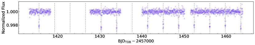
(b) TESS Phase-Folded Light Curve	(d) LCOGT Detrended Light Curves
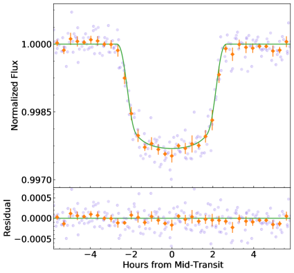
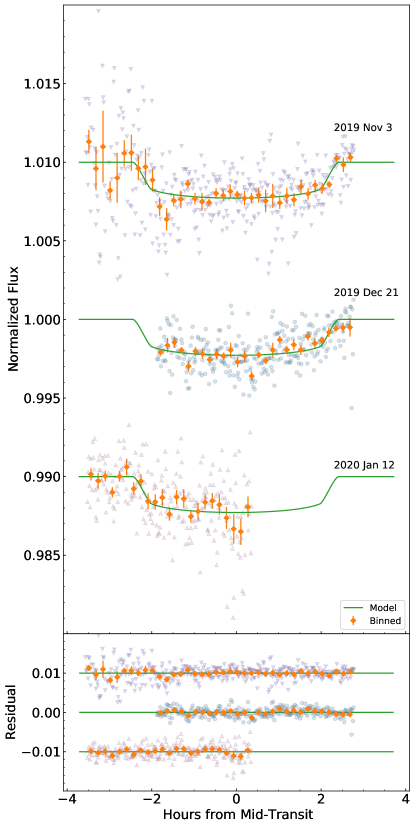
(c) HATSouth Phase-Folded Light Curve

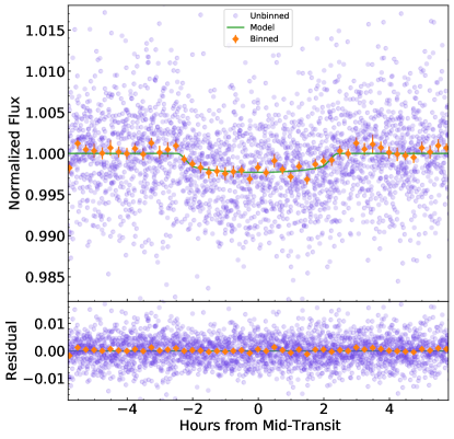
Figure 1: Light curves of TOI-954. The model plotted is the MCMC best-fit solution to the global model. The binned points indicate the mean of each bin, with error bars representing the standard error of the mean. (a) TESS detrended 30 minute cadence light curve. (b) TESS detrended and phase-folded 30 minute cadence light curve after correcting for dilution (Section 2.1.3), focusing on the transit. The bins are 20 minutes. (c) HATSouth TFA detrended and phase-folded light curve after correcting for dilution (Section 2.1.3), focusing on the transit. The bins are 15 minutes. The $y$-axes are restricted for the convenience of presentation, although the outliers are included in the per-bin calculations. (d) LCOGT detrended light curves. The bins are 10 minutes.

TESS observed TOI-954 in sector 4 (UT 2018 October 18–November 15) on camera 2 CCD 2 and in sector 5 (UT 2018 November 15–December 11) on camera 2 CCD 1 with a 30 minute cadence in the full-frame images (FFIs). The MIT Quick Look Pipeline (QLP; Huang et al., 2020a, b) detected the candidate with a signal–to–pink noise ratio of $52.4$. The candidate showed consistent transit depths in all five apertures used by QLP and appeared to be on target in the difference image analysis. The TESS Science Office released the candidate as a TESS object of interest (TOI) after deeming it to have passed all of the vetting criteria (Guerrero et al., 2020).

We used the SPOC-calibrated FFIs (Jenkins et al., 2016), obtained from the TESSCut service (Brasseur et al., 2019), to produce the detrended light curve used in this paper. We used a 45 pixel aperture (a $7\times 7$ square without the four pixels at its corners) centered on the target. This aperture included an unresolved nearby star TIC 44792537 ($\Delta T=3.29$, $48.\mathrm{″}5$ separation, $\mathrm{PA}=$$$) from the TESS Input Catalog (TIC 8; Stassun et al., 2019), which we would correct for by simultaneously fitting a dilution factor in the global model (Section 3.3). We rejected outliers due to spacecraft momentum dumps using the pointing quaternion time series. We also rejected cadences affected by stray light from Earth between JD $2,458,422.2$ and $2,458,423.5$ in orbit 15 (sector 4; Fausnaugh et al., 2019a). No such stray light contamination affected camera 2 in Sector 5 (Fausnaugh et al., 2019b). Orbit 15 was also affected by an instrument anomaly that prevented data collection from JD $2,458,418.54$ to $2,458,421.21$ (Fausnaugh et al., 2019a). We detrended the light curve by simultaneously modeling the spacecraft systematics, transits, and low-frequency variability following Vanderburg et al. (2016). As TESS observed the last transit of TOI-954 b close to the spacecraft’s perigee, the light curve was affected by excessive systematic noise, so we removed that transit from our subsequent analysis to obtain a more accurate transit depth.

2.1.2 K2 Photometry

(a) K2 Campaign 12 Long-Cadence Detrended Light Curve

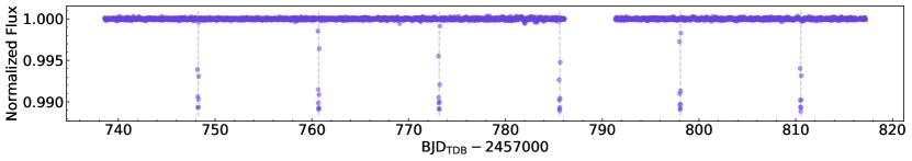
(b) K2 Campaign 19 Short-Cadence Detrended Light Curve

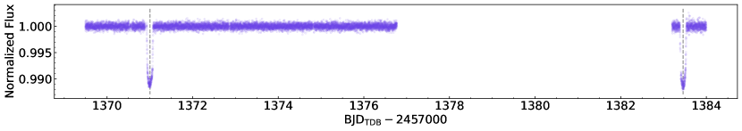
       (c) K2 Campaign 12 Long-Cadence Phase-Folded Light Curve (d) PEST Light Curve                   

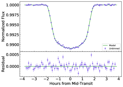
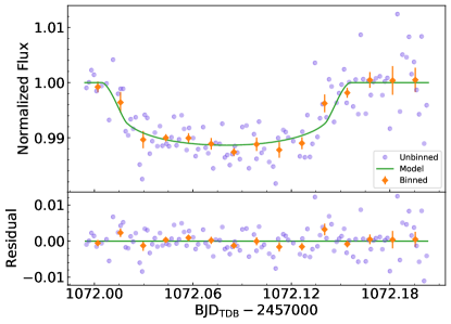
(e) K2 Campaign 19 Short-Cadence Detrended Light Curves

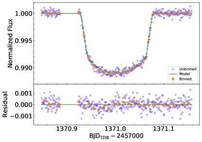
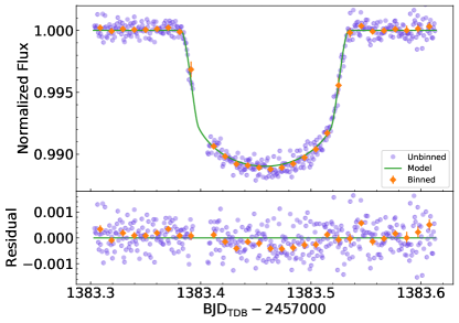
Figure 2: Light curves of K2-329. The model plotted is the MCMC best-fit solution to the global model. (a) K2 campaign 12 long-cadence detrended light curve. (b) K2 campaign 19 short-cadence detrended light curve. (c) K2 campaign 12 long cadence detrended and phase-folded light curve. The noise is estimated from the out-of-transit portions of the light curve. (d) PEST observations. The binned points indicate the mean of each bin (20 minutes), with error bars representing the standard error of the mean. (e) K2 Campaign 19 short cadence detrended light curves. The two transits covered by this campaign are shown side by side. The binned points indicate the mean of each bin (15 minutes). The error bars are the standard error of the mean multiplied by a factor $\beta$ that accounts for the excess red noise (Section 2.1.2). For the two transits, $\beta\approx 1.3$ and $1.6$, respectively.

The object K2-329 was observed in K2 campaign 12 (UT 2016 December 15–2017 March 4) with the 29.4 minute long cadence as part of four GO programs. It was also observed during campaign 19 (UT 2018 August 30–September 26) as part of four long-cadence and one short-cadence ($58.3\text{\,}\mathrm{s}$) guest observer programs.

We initially identified the planet candidate in a box least-squares (BLS) search (Kovács et al., 2002; Vanderburg et al., 2016) of light curves produced by Vanderburg & Johnson (2014) in K2 data from campaign 12. After identifying the planet candidate, we rederived the campaign 12 light curve by simultaneously modeling the spacecraft systematics, transits, and low-frequency variability following Vanderburg et al. (2016).

We took a more custom approach to reducing the campaign 19 data. By the time K2 began executing this campaign, it was critically low on fuel, so the spacecraft exhibited erratic pointing behavior and was only able to observe for about a month before completely exhausting its fuel reserves (K2 Science Office, 2020, accessed on 2020 March 4). Nevertheless, K2 managed to achieve fairly typical pointing performance for about a week between UT 2018 September 8 and 15, during which time K2-329 b transited once. We reduced the data collected during this time interval as usual, producing a first-pass light curve following Vanderburg & Johnson (2014) and refining the systematics correction with a simultaneous fit to the transit of K2-329 b, systematics, and low-frequency variability (Vanderburg et al., 2016).

After UT 2018 September 15, K2’s thruster corrections became less effective, and its pointing began to drift farther and less predictably than usual. We managed to recover a second usable transit of K2-329 b before the end of campaign 19 by performing a simplified systematics correction to a 0.8 day window of data surrounding K2-329 b’s transit. Here again, we simultaneously fit the transit of K2-329 b with a model for stellar variability and K2 pointing systematics. This time, however, we did not attempt to separate the stellar variability from the spacecraft’s pointing drift systematics and modeled both with an aggressive basis spline (with knots spaced every 0.2 days instead of the typical 0.75 days used in a standard K2 reduction), introducing a discontinuity when K2 fired its thrusters (which only happened once during the 0.8 day window). We subtracted the best-fit spline from the original light curve to yield a systematics-free transit.

We estimated the excess red noise affecting the two transits in the Campaign 19 short cadence data following the method described by Winn et al. (2008). We calculated the $\beta$ factor (the effective increase to flux uncertainty due to time-correlated noise) to be $1.3$ for the first transit and $1.6$ for the second, at a timescale comparable to the transit duration. Thus, we multiplied our white-noise estimates for the two transits by their respective $\beta$ factors to obtain the photometric uncertainties we used to calculate the global model posterior (Section 3.3).

2.1.3 Ground-based Follow-up Photometry

Table 2: HATSouth Photometric Measurements of TOI-954

$\mathrm{BJD}_{\mathrm{TDB}}$		Raw Mag.		EPD Mag.		TFA Mag.	Uncertainty	Flag
${}-$2,400,000$$
56983.74903	10.41281	10.35094	10.34490	0.00121	0
56983.75455	10.40697	10.34580	10.34342	0.00121	1
56983.75856	10.40240	10.33414	10.34393	0.00121	0
56983.76259	10.39569	10.32704	10.33661	0.00120	1
56983.76884	10.39573	10.34297	10.34667	0.00121	0
56983.77290	10.40901	10.33885	10.34718	0.00121	0
56983.77695	10.40787	10.34479	10.34520	0.00121	0
56983.78253	10.40622	10.33925	10.33945	0.00121	1
56983.78654	10.40170	10.33649	10.33636	0.00121	1
56983.79106	10.40960	10.34238	10.34526	0.00121	0
56983.79659	10.41026	10.34137	10.34823	0.00121	1
56983.80074	10.41835	10.35022	10.34657	0.00122	0
56983.80476	10.41969	10.34276	10.34678	0.00122	0
56983.81011	10.41058	10.32626	10.34037	0.00121	0
56983.81468	10.42444	10.36145	10.35338	0.00122	1
56983.81878	10.42908	10.36117	10.35667	0.00122	0
56983.82426	10.42465	10.35300	10.34349	0.00122	1
56983.82834	10.42461	10.34070	10.34959	0.00122	1
56983.83246	10.43064	10.34189	10.35611	0.00123	0
56983.83846	10.42909	10.34239	10.34314	0.00122	0
56983.84263	10.43798	10.34189	10.34984	0.00123	0
56983.84664	10.43480	10.33644	10.34282	0.00123	0
56983.85218	10.44484	10.34619	10.34190	0.00124	0
56983.85624	10.45349	10.34244	10.34576	0.00124	0
56983.86080	10.52435	10.33869	10.34762	0.00129	0
56983.86621	10.48563	10.34870	10.34910	0.00130	0
56983.87025	10.46183	10.33230	10.35159	0.00136	0
56984.51946	10.47864	10.36408	10.34731	0.00129	0
56984.52352	10.46848	10.35617	10.34055	0.00126	0
56984.52758	10.46211	10.34552	10.33378	0.00125	0
56984.53352	10.45185	10.32801	10.33251	0.00124	1
56984.53812	10.44663	10.32807	10.33958	0.00123	0
56984.54214	10.45214	10.34555	10.34681	0.00124	0
56984.54819	10.44286	10.34677	10.33815	0.00123	0
56984.55233	10.43931	10.33513	10.34743	0.00123	0
56984.55643	10.44049	10.34325	10.33722	0.00123	1
56984.56297	10.44801	10.35086	10.34400	0.00123	0
56984.56709	10.44393	10.34679	10.34967	0.00123	1
56984.57119	10.43688	10.34890	10.34800	0.00123	0
56984.57646	10.44848	10.36341	10.35508	0.00123	1
56984.58053	10.43158	10.35575	10.34443	0.00123	0

Note. — Two detrended magnitudes are given: one using the external parameter decorrelation (EPD; Bakos et al., 2010) method and one using the TFA (Kovács et al., 2005). A nonzero flag value indicates that an observation is affected by anomalously high systematics and excluded from the global model.

(This table is available in its entirety in machine-readable form.)

The HATSouth (Bakos et al., 2013) survey observed TOI-954 before TESS launched, for a total of $36,396$ observations in the $r$ band at an average cadence of 6 minutes from UT 2014 September 9 to 2015 March 6. The star was slightly saturated for the HATSouth observation, but with the help of the trend-filtering algorithm (TFA; Kovács et al., 2005), we were able to pick up the signal in the light curve. While we were not able to use the HATSouth light curve to confirm whether the transit is on target, its long baseline helped us improve the precision of the planet’s orbital period by an order of magnitude. We listed the measurement data in Table 2.

The object TOI-954 was also observed as part of the TESS Follow-up Program (TFOP). We attempted to observe an ingress on UT 2019 August 3 from the $0.7\text{\,}\mathrm{m}$ PlaneWave CDK700 telescope at Maunakea Observatories, Hawaii, stopping at twilight. The limited precision of the light curve prevented us from either confirming or ruling out the ingress, but we were able to rule out that the transit could have been caused by background eclipsing binaries within $40\mathrm{″}$. The light-curve time series can be found on the ExoFOP-TESS website.

A full transit of TOI-954 was observed in the Pan-STARSS $z_{\mathrm{s}}$ band on UT 2019 November 3 and December 21 and 2020 January 12 using a $1.0\text{\,}\mathrm{m}$ telescope at the LCOGT South African Astronomical Observatory (SAAO) node in Sutherland, South Africa. The LCOGT observations were calibrated with the standard BANZAI pipeline, and the light curves were extracted using AstroImageJ (AIJ; Collins et al., 2017). The observation used a $6\mathrm{″}$ aperture, and recovered the expected transit signal. The detrended light curves can also be found on the ExoFOP-TESS website. The UT 2019 December 21 data were not included in the global model fitting (Section 3.3) because they did not contain enough out-of-transit observations to allow us to accurately measure the transit depth.

Table 3: PEST Photometric Measurements of K2-329

HJD${}_{\mathrm{UTC}}-$2,400,000$$		Magnitude	Uncertainty
58071.9943414	12.4795	0.0028
58071.9958805	12.4784	0.0027
58071.9974061	12.4760	0.0027
58071.9989486	12.4769	0.0026
58072.0004769	12.4801	0.0026
58072.0035502	12.4791	0.0026
58072.0065972	12.4786	0.0026
58072.0081422	12.4858	0.0026
58072.0105639	12.4739	0.0026
58072.0136167	12.4806	0.0025
58072.0151562	12.4796	0.0026
58072.0167014	12.4796	0.0026
58072.0182275	12.4880	0.0026
58072.0197626	12.4888	0.0025
58072.0213111	12.4856	0.0026
58072.0228323	12.4875	0.0026
58072.0243530	12.4852	0.0025
58072.0268029	12.4946	0.0025
58072.0283283	12.4975	0.0026
58072.0298796	12.4847	0.0025
58072.0314200	12.4853	0.0025
58072.0329524	12.4924	0.0026
58072.0344828	12.4899	0.0025
58072.0360143	12.4882	0.0025
58072.0375664	12.4909	0.0025
58072.0391149	12.4869	0.0026
58072.0406562	12.4908	0.0025
58072.0431032	12.4904	0.0025
58072.0446452	12.4909	0.0025
58072.0461702	12.4891	0.0025
58072.0477101	12.4850	0.0025
58072.0492365	12.4907	0.0025
58072.0507722	12.4895	0.0025
58072.0523084	12.4847	0.0025
58072.0538298	12.4874	0.0025
58072.0553637	12.4916	0.0025
58072.0568884	12.4872	0.0025
58072.0593443	12.4892	0.0025
58072.0608676	12.4928	0.0025
58072.0624086	12.4914	0.0025

Note. — We present the observation times in HJD_UTC as originally reported; however, they have been converted to $\mathrm{BJD}_{\mathrm{TDB}}$ before inclusion in the global model (Section 3.3), following the methods described by Eastman et al. (2010). The magnitudes reported in this table are not detrended.

(This table is available in its entirety in machine-readable form.)

On UT 2017 November 14, K2-329 was observed by the Perth Exoplanet Survey Telescope (PEST) with 117 observations at $120\text{\,}\mathrm{s}$ cadence in the $R_{\mathrm{c}}$ band. PEST is a $12^{\prime\prime}$ Meade LX200 SCT Schmidt–Cassegrain telescope equipped with an SBIG ST-8XME camera located in a suburb of Perth, Australia. The PEST pipeline automatically reduced and calibrated the images, producing a light curve, which was normalized for transit model fitting (Tan, n.d.). The transit arrived on time, and we were able to recover a full transit of the planet (Figure 2(c)), allowing us to improve the precision of the planet’s orbital period. We report the measurement data in Table 3.

On UT 2018 July 9, K2-329 was also observed by the $24^{\prime\prime}$ telescope at the Peter van de Kamp Observatory of Swarthmore College, Pennsylvania. We made 78 measurements in the $r^{\prime}$ filter with an exposure time of $90\text{\,}\mathrm{s}$. We observed an egress of K2-329 b on the expected target under good sky conditions. We decided to not include this partially observed transit in our global model fitting (Section 3.3).

2.2 Spectroscopy

We now describe the spectroscopic observations we use to confirm the planets of TOI-954 and of K2-329. A summary of those observations can be found in Table 4.

Table 4: Summary of Spectroscopic Observations

Instrument	UT Date(s)	No. Spectra	Resolution	S/N Range	Wavelengths	Jitter		$\gamma$
			$\Delta\lambda/\lambda/1000$	($5000\text{\,}\mathrm{\SIUnitSymbolAngstrom}$)	($\mathrm{\SIUnitSymbolAngstrom}$)	($\mathrm{m}\text{\,}{\mathrm{s}}^{-1}$)		($\mathrm{m}\text{\,}{\mathrm{s}}^{-1}$)
TOI-954
ANU $2.3\text{\,}\mathrm{m}$	2019 Feb 18–22	3	23	49.6–75.8	3900–6700	…		…
CHIRON	2019 Feb 22–27	5	80	67.7–76.1	4100–8700	$6.6$	${}_{-4.7}^{+9.7}$	$-8826.0$	$\pm 7.3$
CORALIE	2019 Aug 19–Sep 30	19	60	10.0–31.7	3900–6800	$4.9$	${}_{-3.3}^{+4.2}$	$-7347.2$	${}_{-2.9}^{+3.0}$
HARPS	2019 Sep 27–30	4	115	33.6–80.4	3780–6910	$2.5$	${}_{-1.8}^{+4.3}$	$-7321.4$	$\pm 2.1$
Minerva-Australis	2019 Sep 8–Nov 10	12	80	…	5000–6300	$16.0$	${}_{-4.0}^{+5.7}$	$8.2$	${}_{-4.8}^{+5.5}$
PFS	2019 Jul 11–Sep 15	8	130	45–75	3910–7340	$6.8$	${}_{-2.2}^{+3.5}$	$-14.3$	${}_{-2.6}^{+2.9}$
TRES	2019 Mar 1	1	44	30.3	3850–9096	…		…
K2-329
FEROS	2017 Oct 14–2018 Jul 15	27	48	45–55	3500–9200	$17.0$	${}_{-2.8}^{+3.4}$	$-16999.0$	${}_{-4.2}^{+4.1}$
FIES	2017 Aug 16 and 18	2	67	…	3650–9125	…		…
HARPS	2017 Nov 6–2018 Sep 6	13	115	17–35	3780–6910	$5.0$	${}_{-3.1}^{+3.8}$	$-16982.9$	$\pm 2.8$
PFS	2018 May 24–Oct 26	10	130	30–90	3910–7340	$3.7$	${}_{-1.2}^{+1.7}$	$0.8$	$\pm 1.4$
TRES	2017 Sep 10 and 28	2	44	26.8–31.3	3850–9096	…		…

Note. — The jitter parameter is added in quadrature to the reported RV uncertainties in Table 5 and Table 6. The $\gamma$ parameter is a constant offset added to RV measurements of a given RV instrument. The jitter and $\gamma$ values are empirically determined by a global model fit for each star system (see Section 3.3).

2.2.1 Reconnaissance Spectroscopy

Three spectra of TOI-954 were taken with the echelle spectrograph on the Australia National University (ANU) $2.3\text{\,}\mathrm{m}$ telescope for TOI-954 from UT 2019 February 18 to 2019 February 22, covering the wavelength region of $39006700\text{\,}\mathrm{\SIUnitSymbolAngstrom}$ with a spectral resolution $R\approx$23,000$$. These spectra can be found on the ExoFOP-TESS website. The observations suggested that there was no RV variation on the order of $500\text{\,}\mathrm{m}\text{\,}{\mathrm{s}}^{-1}$. We therefore moved on to higher-precision instruments for mass measurements of TOI-954 b.

The Tillinghast Reflector Echelle Spectrograph (TRES; Szentgyorgyi, 2004) on the $1.5\text{\,}\mathrm{m}$ telescope at the Fred L. Whipple Observatory in Arizona was used to obtain spectra for both TOI-954 (UT 2019 March 1) and K2-329 (UT 2017 September 10 and 28). TRES is a fiber-fed echelle spectrograph with a spectral resolution of $R\approx$44,000$$ over the wavelength region of $38509100\text{\,}\mathrm{\SIUnitSymbolAngstrom}$. The observing strategy and data reduction process were described by Buchhave et al. (2012). Each spectrum was obtained from a combination of three consecutive observations for optimal cosmic-ray rejection, and the wavelength solution was provided by bracketing ThAr hollow cathode lamp exposures. The TRES spectra used in this paper can be found on the ExoFOP-TESS and ExoFOP-K2 websites.

We did not find evidence of strong stellar activity for either TOI-954 or K2-329 in the TRES spectra. The Ca II H and K emission lines were absent.

The object K2-329 was also observed with the FIbre-fed Echelle Spectrograph (FIES; Frandsen & Lindberg, 1999; Telting et al., 2014) mounted at the $2.56\text{\,}\mathrm{m}$ Nordic Optical Telescope (NOT) of Roque de los Muchachos Observatory (La Palma, Spain). The observations were carried out on 2 nights (UT 2017 August 16 and 18) using the high-resolution fiber, which provides a resolving power of $67,000$ in the wavelength range $36509125\text{\,}\mathrm{\SIUnitSymbolAngstrom}$. The observing strategy follows the one adopted for TRES observations.

2.2.2 Precise RVs

The high-precision RV measurements used in this paper are presented in Table 5 and Figure 3 for TOI-954; those for K2-329 are presented in Table 6 and Figure 4. We now proceed to describe these observations in detail.

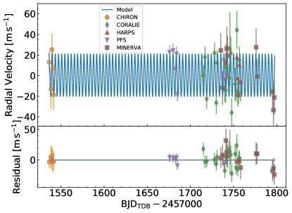
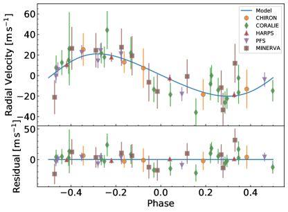
Figure 3: Precise RV measurements of TOI-954. The model plotted is the MCMC median of the global model. A empirically derived per-instrument offset $\gamma$ has been subtracted from the raw RV measurements. The error bars represent the reported uncertainty and the empirically derived per-instrument jitter, added in quadrature. These RV measurements are also listed in Table 5. Top: RV measurements plotted against time. Bottom: phase-folded RV measurements.

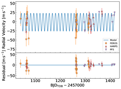
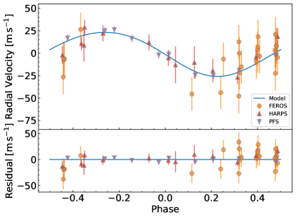
Figure 4: Precise RV measurements of K2-329. The model plotted is the MCMC median of the global model. A empirically derived per-instrument offset $\gamma$ has been subtracted from the raw RV measurements. The error bars represent the reported uncertainty and the empirically derived per-instrument jitter, added in quadrature. These RV measurements are also listed in Table 6. Top: RV measurements plotted against time. Bottom: phase-folded RV measurements.

Table 5: Precise RV Measurements of TOI-954

BJD		RV		Uncertainty	Instrument
		($\mathrm{m}\text{\,}{\mathrm{s}}^{-1}$)		($\mathrm{m}\text{\,}{\mathrm{s}}^{-1}$)
2458536.59568	-8812.91816	8.13894	CHIRON
2458538.60658	-8839.10797	17.70062	CHIRON
2458539.60827	-8800.58690	14.49605	CHIRON
2458540.59466	-8818.69516	18.01763	CHIRON
2458541.57702	-8844.42831	13.41980	CHIRON
2458714.906319	-7347.17	8.83	CORALIE
2458716.832690	-7329.20	9.01	CORALIE
2458718.846938	-7369.61	8.71	CORALIE
2458727.837791	-7325.22	8.84	CORALIE
2458729.867972	-7373.46	9.72	CORALIE
2458730.875885	-7334.57	11.22	CORALIE
2458739.756150	-7360.71	11.34	CORALIE
2458740.811585	-7361.33	10.84	CORALIE
2458741.835606	-7339.48	10.79	CORALIE
2458744.829962	-7349.56	11.96	CORALIE
2458745.737422	-7321.07	35.27	CORALIE
2458746.749066	-7325.21	14.84	CORALIE
2458747.815505	-7383.09	12.90	CORALIE
2458751.740085	-7355.34	15.11	CORALIE
2458752.761760	-7361.95	9.22	CORALIE
2458753.728396	-7302.87	17.82	CORALIE
2458754.766691	-7365.72	10.48	CORALIE
2458755.885741	-7363.77	9.77	CORALIE
2458756.781573	-7332.19	12.27	CORALIE
2458753.799037	-7303.56	3.63	HARPS
2458754.756737	-7324.01	2.46	HARPS
2458755.813724	-7340.08	1.49	HARPS
2458756.749928	-7310.85	2.72	HARPS
2458735.11924305	32.749	5.2134	MINERVA-Australis
2458737.17597222	-3.6402	4.8895	MINERVA-Australis
2458741.08650462	20.146	9.9089	MINERVA-Australis
2458742.09328703	34.614	13.336	MINERVA-Australis
2458743.08164351	27.424	10.512	MINERVA-Australis
2458758.09859953	1.6529	9.5847	MINERVA-Australis
2458776.07408564	35.803	8.5726	MINERVA-Australis
2458777.15123842	7.3249	4.8943	MINERVA-Australis
2458795.08677083	-7.3261	5.2078	MINERVA-Australis
2458796.16503472	-25.319	4.4132	MINERVA-Australis
2458797.08497685	-12.976	4.3832	MINERVA-Australis
2458798.21734953	-38.352	4.4889	MINERVA-Australis
2458675.92609	8.36	1.44	PFS
2458679.92171	10.10	1.17	PFS
2458682.90503	-8.29	1.08	PFS
2458683.94257	6.87	1.37	PFS
2458684.94079	-32.33	0.90	PFS
2458737.88787	-18.21	1.34	PFS
2458738.83838	0.00	1.27	PFS
2458741.83181	-14.90	1.13	PFS

Note. — The RVs given represent absolute relative motion to the solar system barycenter, except for those from Minerva-Australis and PFS, where the mean relative motion has been subtracted. See Table 4 for the constant RV offsets derived by the global model for each instrument.

(This table is available in machine-redable form.)

Table 6: Precise RV Measurements of K2-329

BJD		RV		Uncertainty	Instrument
		($\mathrm{m}\text{\,}{\mathrm{s}}^{-1}$)		($\mathrm{m}\text{\,}{\mathrm{s}}^{-1}$)
2458040.70773863	-16990.7	10.5	FEROS
2458063.59792602	-17046.9	9.3	FEROS
2458064.54347944	-17008.4	9.1	FEROS
2458064.61015499	-17001.6	9.5	FEROS
2458065.63009163	-16991.1	10.6	FEROS
2458065.57747400	-16978.0	9.0	FEROS
2458067.51507559	-16972.5	8.1	FEROS
2458073.51680660	-17044.5	7.7	FEROS
2458261.90205817	-17043.0	7.6	FEROS
2458262.90253453	-16999.1	7.5	FEROS
2458262.88111421	-16986.3	8.3	FEROS
2458262.92396402	-17020.9	7.6	FEROS
2458263.90571009	-16992.3	7.6	FEROS
2458263.92368049	-16980.6	7.5	FEROS
2458263.88775467	-16995.1	7.5	FEROS
2458264.85218595	-17021.5	8.9	FEROS
2458264.87014076	-17000.3	8.0	FEROS
2458264.88809828	-16996.0	8.2	FEROS
2458264.83421933	-16995.5	9.1	FEROS
2458265.91063007	-17005.3	8.2	FEROS
2458265.85674146	-17025.6	9.0	FEROS
2458265.89267519	-17006.7	9.3	FEROS
2458265.87470911	-17004.9	8.5	FEROS
2458311.86733030	-17005.6	7.7	FEROS
2458312.83754233	-17014.2	7.1	FEROS
2458313.81862457	-17002.4	7.5	FEROS
2458314.78898939	-17003.7	9.2	FEROS
2458063.53094302	-17009.9	5.2	HARPS
2458064.52324815	-16987.5	6.8	HARPS
2458066.52560427	-16985.0	8.6	HARPS
2458067.55479447	-16972.1	5.5	HARPS
2458314.80212100	-16964.4	8.5	HARPS
2458316.79691151	-16974.2	17.3	HARPS
2458321.73828811	-16995.9	19.8	HARPS
2458322.75617163	-16993.3	17.2	HARPS
2458323.74986105	-17002.3	12.2	HARPS
2458332.75758515	-16970.9	7.3	HARPS
2458333.80634123	-16988.3	7.3	HARPS
2458366.64961358	-16954.1	6.8	HARPS
2458367.64086452	-16960.8	7.3	HARPS
2458262.89585	-18.20	2.40	PFS
2458264.89722	-1.71	2.67	PFS
2458295.92099	-1.29	1.44	PFS
2458297.89449	-23.55	1.48	PFS
2458298.87651	-24.14	1.51	PFS
2458355.79845	26.91	1.51	PFS
2458406.56625	17.06	2.02	PFS
2458408.56428	-0.47	2.01	PFS
2458415.55544	17.61	1.71	PFS
2458417.55814	25.62	2.11	PFS

Note. — The RVs given represent absolute relative motion to the solar system barycenter, except for those from PFS, where the mean relative motion has been subtracted. See Table 4 for the constant radial velocity offsets derived by the global model for each instrument.

(This table is available in machine-redable form.)

One of our main sources of precise RV data was the iodine-fed Planet Finder Spectrograph (PFS; Crane et al., 2006, 2008, 2010) on the $6.5\text{\,}\mathrm{m}$ Magellan II Telescope at Las Campanas Observatory in Chile. In 2019 July and September, TOI-954 was observed for a total of eight RVs with a 20 minute exposure time for TESS follow-up. The iodine data and iodine-free templates were taken through a $0.\mathrm{″}3$ slit, resulting in $R\approx$130,000$$. The mean internal uncertainty was $1.2\text{\,}\mathrm{m}\text{\,}{\mathrm{s}}^{-1}$, and the signal-to-noise ratio (S/N) ranged from 45 to 75 in the iodine region at the peak of the blaze. Between 2018 May and October, K2-329 was observed for a total of 10 RVs for K2 follow-up. The same $0.\mathrm{″}3$ slit was used with $3\times 3$ binning, resulting in $R\approx$43,000$$. The exposure times ranged from 33 to 50 minutes, achieving an S/N of ${\sim}\mspace{2.0mu}$30–90 in the iodine region at the peak of the blaze and a mean internal uncertainty of $1.9\text{\,}\mathrm{m}\text{\,}{\mathrm{s}}^{-1}$. All PFS data were reduced with a custom IDL pipeline that flat-fielded, removed cosmic rays, and subtracted scattered light. Further details about the iodine cell RV extraction method can be found in Butler et al. (1996).

The High Accuracy Radial velocity Planet Searcher (HARPS; Mayor et al., 2003) also contributed a significant portion of the precise RV data used in this paper. HARPS is fiber-fed by the Cassegrain focus of the $3.6\text{\,}\mathrm{m}$ telescope at La Silla Observatory in Chile. We obtained four spectra of TOI-954 during consecutive nights, UT 2019 September 27–30, in good seeing conditions (${\sim}\mspace{2.0mu}$$1.\mathrm{″}0$). The exposure time was 20 minutes, leading to an S/N of 33.6–80.4 at $5000\text{\,}\mathrm{\SIUnitSymbolAngstrom}$. HARPS also observed K2-329 for two pairs of consecutive nights in UT 2017 November, five nights in UT 2018 July, and a pair of consecutive nights each in UT 2018 August and September, for a total of 13 spectra. We adopted exposure times of $15001800\text{\,}\mathrm{s}$ for K2-329, which resulted in spectra with an S/N per resolution element of 17–35.

The rest of the spectrographs observed either one of the two planets. The FEROS spectrograph (Kaufer et al., 1999), mounted on the MPG/ESO $2.2\text{\,}\mathrm{m}$ telescope at La Silla observatory in Chile, observed 27 spectra of K2-329 at $R\approx$48,000$$ between UT 2017 October 14 and 2018 July 15. Each spectrum achieved an S/N of 50 per spectral resolution element with exposure times of $1200\text{\,}\mathrm{s}$. The instrumental drift was determined via comparison with a simultaneous fiber illuminated with a ThAr+Ne lamp. The data were processed with the CERES suite of echelle pipelines (Brahm et al., 2017), which produce RVs and bisector spans in addition to reduced spectra.

The final two spectrographs observed TOI-954 only. We obtained a total of seven spectra using the CHIRON echelle spectrograph (Tokovinin et al., 2013) on the SMARTS $1.5\text{\,}\mathrm{m}$ telescope located at the Cerro Tololo Inter-American Observatory (CTIO), Chile, between UT 2019 February 22 and 27. CHIRON was fed via an image slicer and a fiber bundle, yielding a resolving power of $R\approx$80,000$$ over the wavelength range of $41008700\text{\,}\mathrm{\SIUnitSymbolAngstrom}$. Our observations were obtained at an exposure time of $900\text{\,}\mathrm{s}$, achieving an average S/N of 65 over the Mg b lines. The RVs were derived via a least-squares deconvolution between the observed spectra and synthetic nonrotating spectral templates generated via the ATLAS9 stellar models (Castelli & Kurucz, 2004).

Last but not least, we observed TOI-954 with the fiber-fed spectrograph CORALIE ($R\approx 60000$, Queloz et al., 2001) on the Swiss $1.2\text{\,}\mathrm{m}$ Euler telescope located at La Silla Observatory (ESO, Chile). We acquired 19 RV measurements between UT 2019 August 19 and September 29, with the first CORALIE fiber on the star and the second one connected to a Fabry–Pérot etalon for simultaneous wavelength calibration, yielding an S/N of 10.0–31.7 over the wavelength range of $39006800\text{\,}\mathrm{\SIUnitSymbolAngstrom}$. The RVs were computed for each epoch by cross-correlating with a G2 mask using the standard CORALIE Data Reduction Software (DRS; Pepe et al., 2002), which also produced various line-profile diagnostics such as cross-correlating bisector span, FWHM, and contrast. The typical RV uncertainty achieved for the star was $11\text{\,}\mathrm{m}\text{\,}{\mathrm{s}}^{-1}$.

We observed TOI-954 with the Minerva-Australis telescope array (Addison et al., 2019, 2020) at Mt. Kent Observatory in Queensland, Australia, for 12 RV measurements between UT 2019 September 8 and November 10. Minerva-Australis is a set of PlanetWave CDK700 telescopes connected by fibers to a single KiwiSpec R4-100 spectrograph (Barnes et al., 2012), yielding a resolution of $R\approx 80,000$ with wavelength coverage from $50006300\text{\,}\mathrm{\SIUnitSymbolAngstrom}$. We calculated the radial velocities using least-squares analysis, correcting for instrumental drift with simultaneous observations of a ThAr lamp. We measured an RMS scatter of $18\text{\,}\mathrm{m}\text{\,}{\mathrm{s}}^{-1}$ from the median Markov Chain Monte Carlo (MCMC) solution to the global model (Section 3.3). We discarded one RV measurement made on UT 2019 November 10 ($\mathrm{BJD}_{\mathrm{TDB}}$ $2,458,798.2173$) for the global model fitting (Section 3.3) because it was a $>4\sigma$ outlier.

2.3 High Spatial Resolution Imaging

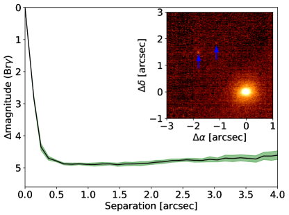
Figure 5: The VLT/NaCo image of TOI-954 and sensitivity to background companions at close separations. The sensitivity is shown in the main plot, and the inset shows the central portion of the image itself, with the star offset so that the companions can be more clearly seen. Both visual companions are highlighted with blue arrows. The northern companion is a marginal detection of just $3\sigma$, but the southern companion is well above our detection threshold.

We collected AO images of TOI-954 with VLT/NAOS–CONICA (NaCo; Lenzen et al., 2003; Rousset et al., 2003) on UT 2019 September 14 to search for nearby companions. Nine exposures were collected in the Br$\gamma$ filter, each with an integration time of $30\text{\,}\mathrm{s}$. The telescope was dithered by $2\mathrm{″}$ between each individual image. We used a custom IDL code to process the data following standard practice; bad pixels were removed, data were flat-fielded, a sky background was constructed from the dithered frames and subtracted, and the images were finally aligned and coadded. When visually inspecting the data, we found two visual companions: a firm detection of a companion at $2.\mathrm{″}3$ and a marginal detection of a companion at $2.\mathrm{″}1$, at approximately $3\sigma$. Both companions are to the NE of the target and mutually separated by $781\text{\,}\mathrm{mas}$.

We calculate our sensitivity to background stars by injecting model companions into the data and scaling their brightness until they are detected at $5\sigma$. This process is repeated at a range of angles and radii, and the final sensitivity is averaged azimuthally. The brighter companion is masked out during this sensitivity calculation. A plot of the sensitivity to companions is shown in Figure 5, which also includes a thumbnail image of the target with the two companions highlighted.

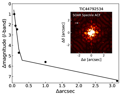
Figure 6: SOAR observation of TOI-954. The $5\sigma$ detection sensitivity is plotted with the speckle imaging ACF inset. The companion is mirrored in the ACF, but its true position ($\mathrm{PA}=$$$) is marked with an arrow.

We also searched for nearby sources to TOI-954 with SOAR speckle imaging (Tokovinin, 2018) on UT 2019 August 12, observing in a similar visible bandpass as TESS. Further details of the observations are available from Ziegler et al. (2020). Confirming the finding from NaCo, a faint companion ($\delta m_{I}=6.2$) was detected at a separation of $2.\mathrm{″}35$. The contamination from the star is negligible, implying a planetary radius correction factor of $1.002$ due to dilution of the transit depth. The $5\sigma$ detection sensitivity and the speckle autocorrelation function (ACF) from the SOAR observation are plotted in Figure 6.

(a) 2017 August 14
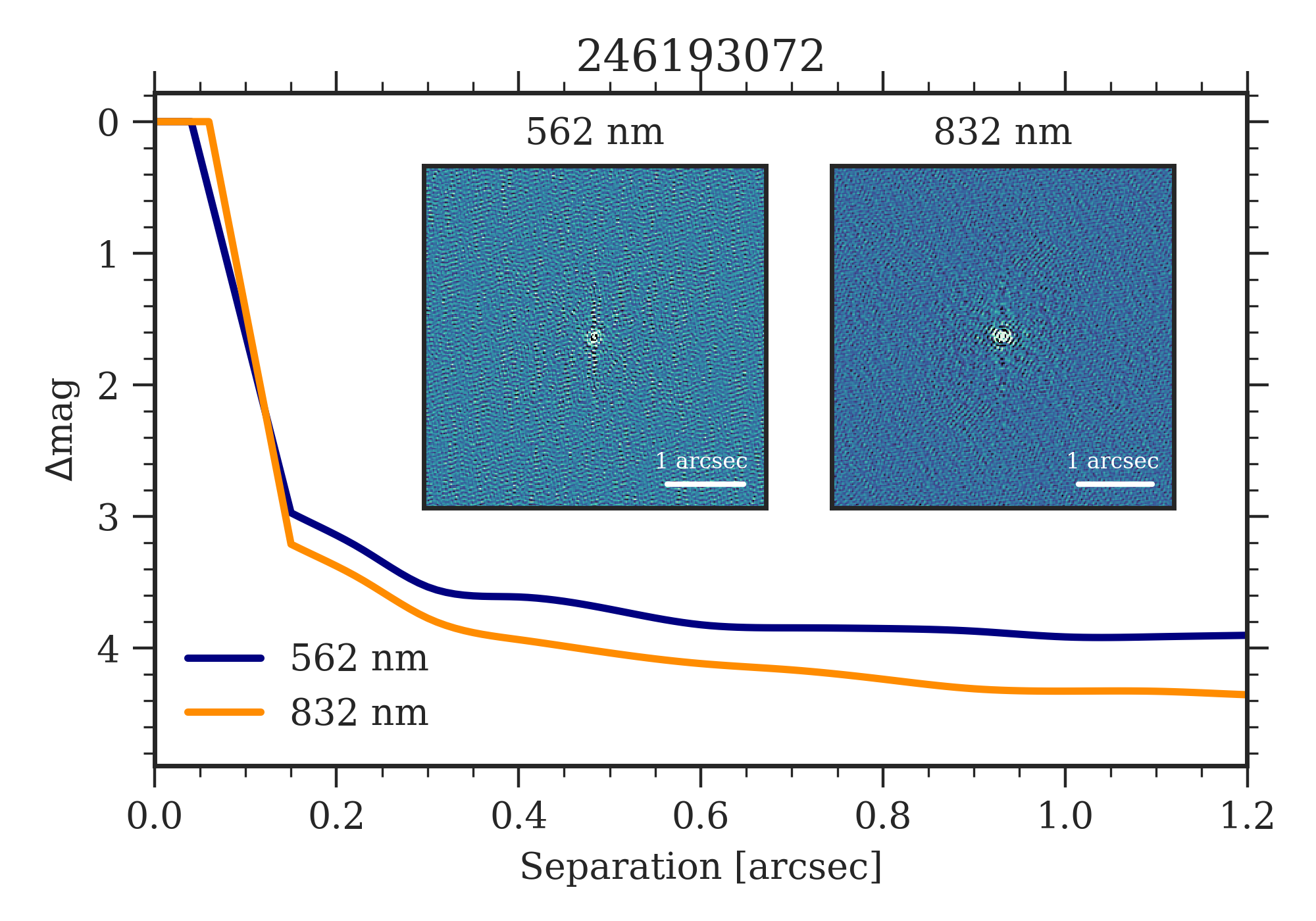
(b) 2017 September 5

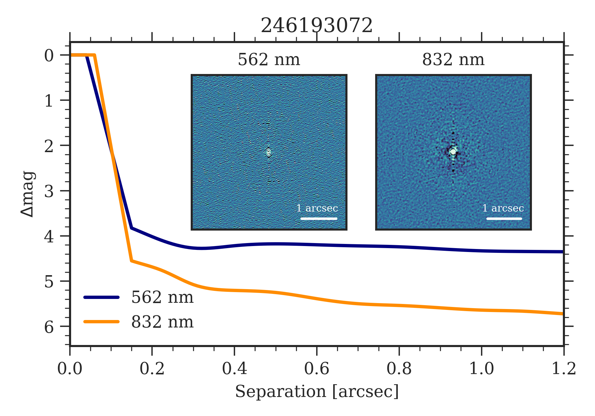
Figure 7: WIYN observations of K2-329 on UT 2017 August 14 (top) and UT 2017 September 5 (bottom). The $5\sigma$ contrast curves are plotted with the reconstructed images. No companions are detected.

We acquired speckle imaging data of K2-329 with the NN-Explore Exoplanet Stellar Speckle Imager (NESSI; Scott et al., 2018) installed on the $3.5\text{\,}\mathrm{m}$ telescope at WIYN Observatory on 2 nights, UT 2017 August 14 and September 5. The observations were in two passbands, $562832\text{\,}\mathrm{n}\mathrm{m}$. Plots of the contrast curves with the reconstructed images inset can be found in Figure 7. The conditions were slightly more favorable on September 5, which led to better contrast in both channels. No companions were detected.

3 Analysis

3.1 Confirmation of TOI-954 b and K2-329 b

Our follow-up observations rule out common astrophysical false positives that may be mistaken for a transiting planet. The transit signals for both TOI-954 b and K2-329 b are confirmed to be on target by ground-based observations. We have also detected strong RV signals matching the transit-derived orbital periods for both planets. We can rule out that the TOI-954 b signal is contaminated by the stars at a separation of ${\sim}\mspace{2.0mu}$$2\mathrm{″}$ because the PFS slit ($0.\mathrm{″}3$) excludes those sources. Speckle imaging did not detect any stars that could contaminate the signal of K2-329 b. Therefore, we confirm the two planets with high confidence.

3.2 Stellar Parameters

3.2.1 Reconnaissance Spectra

We used the Stellar Parameter Classification tool (SPC; Buchhave et al., 2012) to extract stellar parameters such as $T_{\mathrm{eff}}$, $\log g$, metallicity, and $v\sin i$ from the TRES spectra. We were able to determine that TOI-954 is slightly evolved off the main sequence and that K2-329 is a main-sequence star with $T_{\mathrm{eff}}=$5359\pm 50\text{\,}\mathrm{K}$$, $\log g=4.6\pm 0.1$, $[\mathrm{Fe/H}]=0.16\pm 0.08$, and $v\sin i=$1.9\pm 0.5\text{\,}\mathrm{km}\text{\,}{\mathrm{s}}^{-1}$$.

Because we only obtained a relatively low S/N spectrum for TOI-954 from TRES, we opted to use the stellar parameters derived from the average of seven CHIRON spectra. The CHIRON spectra were calibrated against a library of ${\sim}\mspace{2.0mu}$$10,000$ observed spectra classified by the SPC pipeline, interpolated via a gradient-boosting regressor. We derived $T_{\mathrm{eff}}=$5710\pm 51\text{\,}\mathrm{K}$$, $\log g=4.00\pm 0.05$, $[\mathrm{Fe/H}]=0.21\pm 0.05$, and $v\sin i=$5.6\pm 0.5\text{\,}\mathrm{km}\text{\,}{\mathrm{s}}^{-1}$$ for TOI-954 from the CHIRON spectra.

As a sanity check, we also determined the stellar parameters of K2-329 from the coadded FIES spectra. We followed the method outlined in Gandolfi et al. (2017) and used a customized IDL software suite that fitted spectral features sensitive to different photospheric parameters with ATLAS 9 model atmospheres (Castelli & Kurucz, 2004). The results corroborated the stellar parameters derived from the TRES spectra to within $1\sigma$.

The $T_{\mathrm{eff}}$ and $[\mathrm{Fe/H}]$ of both stars are used as Gaussian priors in our global model fitting (Section 3.3). The $\log g$ values, however, are not used to constrain the global model and thus serve as an independent check on the stellar density as constrained by the transit light curve.

3.2.2 Spectral Energy Distribution

(a) TOI-954

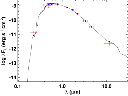
(b) K2-329

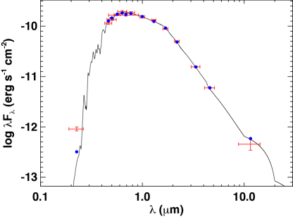
Figure 8: The SED for TOI-954 (top) and K2-329 (bottom). Red symbols represent the observed photometric measurements, where the horizontal bars represent the effective width of the passband. Blue symbols are the model fluxes from the best-fit Kurucz atmosphere model (black).

As an independent check on the derived stellar parameters, we performed an analysis of the broadband spectral energy distribution (SED) together with the Gaia parallax in order to determine an empirical measurement of the stellar radius, following the procedures described by Stassun & Torres (2016) and Stassun et al. (2017, 2018). We obtained the $B_{\mathrm{T}}V_{\mathrm{T}}$ magnitudes from Tycho-2, the BVgri magnitudes from APASS, the $JHK_{S}$ magnitudes from the Two Micron All Sky Survey (2MASS), the W1–W3 magnitudes from the Wide-field Infrared Survey Explorer, the $G$ magnitude from Gaia, and the Galaxy Evolution Explorer near-UV flux. Together, the available photometry spanned the full stellar SED over the wavelength range $0.210\text{\,}\mathrm{\SIUnitSymbolMicro m}$ (see Figure 8).

We performed separate fits for TOI-954 and K2-329 using Kurucz stellar atmosphere models with the priors on effective temperature ($T_{\mathrm{eff}}$), surface gravity ($\log g$), and metallicity ($[\mathrm{Fe/H}]$) from the reconnaissance spectroscopic values. The remaining free parameter was the extinction ($A_{V}$), which we limited to the maximum line-of-sight extinction from the Schlegel et al. (1998) dust maps. The resulting fits were very good (Figure 8), with a reduced $\chi^{2}=2.3$ and a best-fit extinction of $A_{V}=0.06\pm 0.06$ for TOI-954 and a reduced $\chi^{2}=1.58$ and a best-fit $A_{V}=0.09\pm 0.03$ for K2-329. We adopted these $A_{V}$ values as Gaussian priors for bolometric corrections in our global model (Section 3.3). The NUV flux of TOI-954 implies a modest level of chromospheric activity.

Integrating the unextincted model SEDs gave a bolometric flux of $F_{\mathrm{bol}}=$(1.975\pm 0.093)\times 10^{-9}\text{\,}\mathrm{erg}\text{\,}{\mathrm{s}}^{-1}\text{\,}{\mathrm{cm}}^{-2}$$ at Earth for TOI-954 and $F_{\mathrm{bol}}=$(2.880\pm 0.033)\times 10^{-10}\text{\,}\mathrm{erg}\text{\,}{\mathrm{s}}^{-1}\text{\,}{\mathrm{cm}}^{-2}$$ at Earth for K2-329. Taking the $F_{\mathrm{bol}}$ and $T_{\mathrm{eff}}$ together with the Gaia parallax, adjusted by $+0.08\text{\,}\mathrm{mas}$ to account for the systematic offset reported by Stassun & Torres (2018), gave stellar radii of $1.898\pm 0.058\text{\,}\mathrm{\mathnormal{R}}_{\mathrm{\odot}}$ for TOI-954 and $0.804\pm 0.017\text{\,}\mathrm{\mathnormal{R}}_{\mathrm{\odot}}$ for K2-329.

3.3 Global Modeling

For each of the TOI-954 and the K2-329 planetary systems, we used the Emcee Python package (Foreman-Mackey et al., 2013) to perform a global MCMC model fit for planet properties, orbital parameters, and stellar properties. We ran the MCMC sampler over $500,000$ iterations for each system, with 350 walkers for TOI-954 and 250 walkers for K2-329. We calculated the integrated autocorrelation time, or roughly the number of iterative steps it takes for a walker chain to generate an independent sample from the posterior distribution, following Goodman & Weare (2010) and empirically found it to be in the range of $750020,000$ steps for the TOI-954 system model and $600011,000$ steps for the K2-329 system model. Based on this autocorrelation timescale, we discarded the first $100,000$ iterations as burn-in.

Table 7: Quadratic Limb-darkening Parameters

Filter	$u_{1}$		$u_{2}$
TOI-954
TESS	$0.25$	${}_{-0.14}^{+0.16}$	$0.29$	${}_{-0.19}^{+0.20}$
$r$	$0.483$	${}_{-0.034}^{+0.033}$	$0.163$	${}_{-0.051}^{+0.053}$
$z_{\mathrm{s}}$	$0.32$	$\pm 0.31$	$0.199$	${}_{-0.058}^{+0.057}$
K2-329
Kepler	$0.535$	$\pm 0.022$	$-0.002$	${}_{-0.045}^{+0.044}$
$R_{\mathrm{c}}$	$0.542$	${}_{-0.033}^{+0.033}$	$0.185$	${}_{-0.059}^{+0.057}$

Note. — In the MCMC global modeling fit, we used the triangle sampling parameterization $(q_{1},q_{2})$ of the quadratic limb-darkening law by Kipping (2013). We used the least-squares values tabulated by Claret (2017) for TESS and Claret et al. (2013) for all other filters as Gaussian priors, taking the average deviation between the least-squares and the flux-conservation methods as the standard error. Here we report the posterior distribution (16th, 50th, and 84th percentiles) of the conventional $(u_{1},u_{2})$ quadratic limb-darkening parameters, converted from the MCMC samples of $(q_{1},q_{2})$.

For each system, we modeled the detrended and normalized light curves (after rejecting out-of-transit outliers $>4\sigma$) with the Batman package (Kreidberg, 2015). In each model, we constrained the impact parameter so that the planet transits (i.e. $|b|<1+$\mathrm{\mathnormal{R}}_{\mathrm{p}}$/$\mathrm{\mathnormal{R}}_{\mathrm{\star}}$$), and the radius of the planet is additionally constrained to be within 0.4 of the stellar radius. We also restricted the eccentricity to be less than $0.9$ because the Kepler solver in Batman may fail at extremely high eccentricities. For each transit in the LCOGT, PEST, and K2 campaign 19 data, we also simultaneously fitted and subtracted a weighted least-squares linear trend across the transit from the model residuals before calculating the $\chi^{2}$ for the model posterior.

We added a variety of additional parameters to improve the light curves’ fit to the data; these additional parameters are reported in Table 1. We included a dilution factor for the TESS light curve with a Gaussian prior centered at $0.0460$ and a width of $0.0046$, which is the theoretical dilution from the unresolved star in our aperture calculated using TESS magnitudes in TIC 8. As the TFA detrending method tended to make the transit depth shallower than the true transit in HATSouth light curves, we included an additional dilution factor in the model with a flat prior in $(0,1)$. To account for possible underestimation of the noise of LCOGT and PEST measurements, we multiplied the quoted LCOGT noise by a factor $\geq 1$ and added a nonnegative jitter term in quadrature to the quoted PEST noise as free parameters in their respective global model. We did not add any additional jitter to either the TESS or K2 light curves because the global model consistently preferred a value of zero during trial runs.

We note that the MCMC posterior solution for the TOI-954 system prefers a value much lower than the prior for the TESS light-curve dilution factor. We believe that this apparent discrepancy arises because the dilution-corrected TESS light curve and the LCOGT light curves imply slightly different transit depths for the planet, which is captured by the global model in the larger uncertainties for the radius of TOI-954 b it reports.

We used the triangular sampling of the quadratic limb-darkening law coefficients recommended by Kipping (2013), and constrained the coefficients using Gaussian priors. The priors were centered on values interpolated using the gradient-boosting regressor in the Scikit-learn package from the least-squares fitted values tabulated by Claret (2017) for TESS and Claret et al. (2013) for all other filters. The posterior distributions of the quadratic limb-darkening parameters are reported in Table 7.

We modeled the corresponding RVs with Radvel (Fulton et al., 2018) in the joint fit. For each spectroscopic instrument, we introduced a constant offset term $\gamma$ to the reported RVs and added a jitter term in quadrature with the reported errors, allowing the model to adjust each freely. The $\gamma$ terms are unconstrained, while the jitter terms are constrained to be nonnegative. Those additional RV parameters are reported in Table 4. We did not find any statistically significant long-term trends in the RV measurements of either star.

To simultaneously constrain stellar properties, we fitted for initial stellar mass, initial stellar metallicity, and age in our global model. Those three parameters served as independent variables of the MIST isochrones (Choi et al., 2016; Dotter, 2016), which we interpolated with the Isochrones Python package (Morton, 2015). We constrained the initial stellar mass to not exceed the valid range for the MIST isochrones $[0.1,300]\,$\mathrm{\mathnormal{M}}_{\mathrm{\odot}}$$ and the stellar age to $[10^{-4},14]\,$\mathrm{Gyr}$$. The isochrone interpolation produced the current mass, metallicity ($[\mathrm{Fe/H}]$), $T_{\mathrm{eff}}$, and $\log g$ of the star, as well as the predicted Gaia absolute magnitudes. The transit light curves implicitly constrained the mass and $\log g$. To account for the theoretical uncertainty of the underlying stellar evolutionary model, we added a random Gaussian noise of 5% to the current stellar mass at each iterative step. We used the values derived from the reconnaissance spectra (CHIRON for TOI-954, TRES for K2-329; see Section 2.2.1) as Gaussian priors for the metallicity and $T_{\mathrm{eff}}$.

We used the three Gaia magnitudes $G$, $G_{\mathrm{RP}}$, and $G_{\mathrm{BP}}$ to constrain the absolute magnitudes obtained from the isochrone interpolation. To apply bolometric corrections to the absolute magnitudes, we randomly drew values of $A_{V}$ extinctions from a normal distribution based on the results of the independent SED analysis described in Section 3.2.2. The isochrone-derived absolute magnitudes were then compared to those computed from the photometric and parallax measurements in Gaia DR2. We added an additional jitter, constrained to within $[0,0.2)$, in quadrature to the three Gaia magnitudes as a free parameter to the model to account for additional systematic uncertainties. As with the independent SED analysis, we added a systematic offset of $+0.082\pm 0.033\text{\,}\mathrm{mas}$ reported by Stassun & Torres (2018) to the Gaia parallaxes.

Table 8: Stellar Parameters

Parameter Unit	TOI-954		K2-329		Source
Identifying Information
$\alpha$ R.A. (J2015.5) h:m:s	$04\mathrm{°}⁤07\mathrm{\prime }⁤45.\mathrm{″}854$		$23\mathrm{°}⁤24\mathrm{\prime }⁤32.\mathrm{″}491$		Gaia DR2
$\delta$ Decl. (J2015.5) d:m:s	$-25\mathrm{°}⁤12\mathrm{\prime }⁤31.\mathrm{″}69$		$-05\mathrm{°}⁤09\mathrm{\prime }⁤50.\mathrm{″}92$		Gaia DR2
2MASS ID	J04074585–2512312		J23243247–0509507		TIC 8
TIC ID	44792534		301258470		TIC 8
	…		246193072		EPIC
Space observations	TESS sectors 4 and 5		K2 campaigns 12 and 19
Parallax mas	$4.242$	$\pm 0.046$	$4.341$	$\pm 0.053$	Gaia DR2
$\mu_{\alpha}$, R.A. proper motion …$\mathrm{mas}\text{\,}{\mathrm{yr}}^{-1}$	$-5.787$	$\pm 0.042$	$14.169$	$\pm 0.063$	Gaia DR2
$\mu_{\delta}$, decl. proper motion …$\mathrm{mas}\text{\,}{\mathrm{yr}}^{-1}$	$-29.623$	$\pm 0.045$	$-12.389$	$\pm 0.052$	Gaia DR2
Photometric Properties
TESS mag	$9.779$	$\pm 0.006$	$11.904$	$\pm 0.006$	TIC 8
Kepler mag	…		12.463		EPIC
$B$ mag	$11.153$	$\pm 0.063$	$13.542$	$\pm 0.070$	TIC 8
$V$ mag	$10.343$	$\pm 0.005$	$12.697$	$\pm 0.080$	TIC 8
$J$ mag	$9.180$	$\pm 0.024$	$11.174$	$\pm 0.023$	TIC 8
$H$ mag	$8.891$	$\pm 0.026$	$10.798$	$\pm 0.028$	TIC 8
$K$ mag	$8.779$	$\pm 0.023$	$10.668$	$\pm 0.023$	TIC 8
$G$ mag	$10.2321$	$\pm 0.0002$	$12.4462$	$\pm 0.0003$	Gaia DR2
$G_{\mathrm{BP}}$ mag	$10.5978$	$\pm 0.0006$	$12.9023$	$\pm 0.0015$	Gaia DR2
$G_{\mathrm{RP}}$ mag	$9.7328$	$\pm 0.0005$	$11.8537$	$\pm 0.0013$	Gaia DR2
JitterG mag	$0.026$	${}_{-0.019}^{+0.052}$	$0.039$	${}_{-0.029}^{+0.080}$	Sampled
Stellar Properties
$T_{\mathrm{eff}}$, effective temperature K	$5710$	${}_{-49}^{+53}$	$5282$	${}_{-39}^{+40}$	Derived
$[\mathrm{Fe/H}]$, metallicity dex	$0.215$	${}_{-0.051}^{+0.050}$	$0.098$	${}_{-0.070}^{+0.065}$	Sampled
$\log g$, surface gravity dex	$3.962$	${}_{-0.024}^{+0.026}$	$4.566$	${}_{-0.021}^{+0.013}$	Derived
$v\sin i$, rotational speed $\mathrm{km}\text{\,}{\mathrm{s}}^{-1}$	$5.6$	$\pm 0.5$	$1.9$	$\pm 0.5$	Spectroscopy
$M_{\star}$, mass $\mathrm{\mathnormal{M}}_{\mathrm{\odot}}$	$1.201$	${}_{-0.064}^{+0.066}$	$0.901$	${}_{-0.049}^{+0.048}$	Sampled
$R_{\star}$, radius $\mathrm{\mathnormal{R}}_{\mathrm{\odot}}$	$1.892$	${}_{-0.076}^{+0.077}$	$0.822$	${}_{-0.024}^{+0.026}$	Derived
$\rho_{\star}$, density $\mathrm{g}\text{\,}{\mathrm{cm}}^{-3}$	$0.249$	${}_{-0.021}^{+0.025}$	$2.30$	${}_{-0.16}^{+0.12}$	Derived
$L_{\star}$, luminosity $L_{\odot}$	$3.43$	${}_{-0.23}^{+0.24}$	$0.473$	${}_{-0.028}^{+0.033}$	Derived
Age Gyr	$6.14$	${}_{-0.30}^{+0.30}$	$1.8$	${}_{-1.3}^{+2.2}$	Sampled

Note. — The values from this work are the medians and 16th and 84th percentiles of the MCMC-derived posterior distribution. All solar-scaled units in this paper are defined and calculated as the recommended nominal values adopted in IAU 2015 Resolution B3 (Prša et al., 2016).

References. — Sampled: this work. Derived: calculated from the sampled parameters with the MIST isochrone models (Dotter, 2016; Choi et al., 2016). Spectroscopy: derived from reconnaissance spectra only; not part of the global model. EPIC: Huber et al. (2016). Gaia DR2: Gaia Collaboration et al. (2018). TIC 8: Stassun et al. (2019).

Table 9: Planetary and System Parameters

Parameter Unit	TOI-954 b		K2-329 b
Sampled Parameters
$T_{c}$, time of conjunction BJD	$2458411.90651$	${}_{-0.00078}^{+0.00084}$	$2457773.157267$	${}_{-0.000075}^{+0.000073}$
$P$, period day	$3.6849729$	${}_{-0.0000028}^{+0.0000027}$	$12.4551225$	$\pm 0.0000031$
$K$, RV semiamplitude $\mathrm{m}\text{\,}{\mathrm{s}}^{-1}$	$20.7$	${}_{-1.9}^{+2.0}$	$24.6$	${}_{-1.8}^{+1.6}$
$\sqrt{e}\sin\omega$	$-0.35$	${}_{-0.20}^{+0.49}$	$0.081$	${}_{-0.094}^{+0.089}$
$\sqrt{e}\cos\omega$	$0.07$	${}_{-0.13}^{+0.06}$	$-0.23$	${}_{-0.08}^{+0.13}$
$b\equiv a\cos{i}/R_{\star}$	$0.56$	${}_{-0.24}^{+0.04}$	$0.364$	${}_{-0.048}^{+0.039}$
$R_{p}/R_{\star}$	$0.0462$	${}_{-0.0023}^{+0.0019}$	$0.09679$	${}_{-0.00057}^{+0.00056}$
Derived Parameters
$T_{14}$, total transit duration hour	$5.09$	${}_{-0.37}^{+0.93}$	$3.621$	${}_{-0.017}^{+0.019}$
$e$, eccentricity	$0.14$	${}_{-0.11}^{+0.18}$	$0.0697$	${}_{-0.040}^{+0.041}$
$e$, eccentricity (95th percentile)	0.37		$0.140$
$\omega$, argument of periastron …degree	$276$	${}_{-174}^{+9}$	$161$	${}_{-30}^{+22}$
$a$, semimajor axis au	$0.04963$	${}_{-0.00090}^{+0.00089}$	$0.1016$	${}_{-0.0019}^{+0.0018}$
$a/R_{\star}$	$5.63$	${}_{-0.17}^{+0.18}$	$26.62$	${}_{-0.61}^{+0.46}$
$i$, inclination degree	$84.4$	${}_{-0.6}^{+2.5}$	$89.22$	${}_{-0.09}^{+0.11}$
$$\mathrm{\mathnormal{M}}_{\mathrm{p}}$\sin i$, minimum mass $\mathrm{\mathnormal{M}}_{\mathrm{J}}$	$0.174$	${}_{-0.017}^{+0.018}$	$0.260$	${}_{-0.022}^{+0.020}$
$\mathrm{\mathnormal{M}}_{\mathrm{p}}$, mass $\mathrm{\mathnormal{M}}_{\mathrm{J}}$	$0.174$	${}_{-0.017}^{+0.018}$	$0.260$	${}_{-0.022}^{+0.020}$
$\mathrm{\mathnormal{R}}_{\mathrm{p}}$, radius $\mathrm{\mathnormal{R}}_{\mathrm{J}}$	$0.852$	${}_{-0.062}^{+0.053}$	$0.774$	${}_{-0.024}^{+0.026}$
$\mathrm{\mathnormal{\rho}}_{\mathrm{p}}$, density $\mathrm{g}\text{\,}{\mathrm{cm}}^{-3}$	$0.35$	${}_{-0.07}^{+0.10}$	$0.694$	${}_{-0.072}^{+0.070}$
Stellar irradiation $\mathrm{erg}\text{\,}{\mathrm{s}}^{-1}\text{\,}{\mathrm{cm}}^{-2}$	$(1.896$	${}_{-0.085}^{+0.090})\times 10^{9}$	$(6.22$	${}_{-0.22}^{+0.30})\times 10^{7}$
$T_{\mathrm{eq}}$, equilibrium temperature K	$1526$	${}_{-164}^{+123}$	$650$	${}_{-70}^{+53}$

Note. — The values given are the medians and 16th and 84th percentiles of the MCMC-derived marginalized posterior distribution. All Jupiter-scaled units in this paper are defined and calculated as the recommended nominal values adopted in IAU 2015 Resolution B3 (Prša et al., 2016). The Jupiter radius $\mathrm{\mathnormal{R}}_{\mathrm{J}}$ is taken to be the equatorial radius.

The resulting posterior distributions show an excellent fit with the observations (Figures 1–4). The final median and 16th, 84th percentile values of the stellar and planetary system parameters are reported in Tables 3.3 and 9. Representative MCMC samples of the posterior distributions for the two models are reported separately in Tables 10 and 13.

We also ran an independent global analysis of the available photometric and RV measurements of K2-329 using EXOFASTv2 (Eastman et al., 2013, 2019). The results of the EXOFASTv2 analysis were consistent ($<1\sigma$) with the analysis described above in this section.

4 Discussion

(a)                                                                    (b)

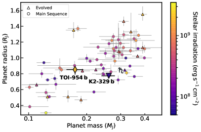
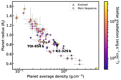
(c)                                                                    (d)

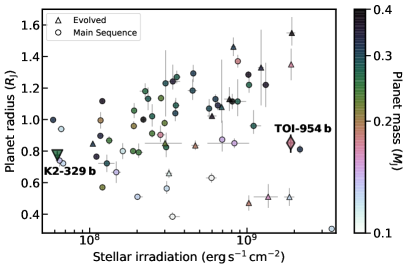
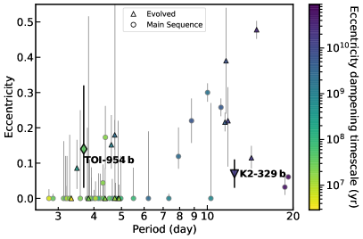
Figure 9: Planets TOI-954 b and K2-329 b compared to planets of similar mass (measured to better than 50%) and period ($0.1\leq$\mathrm{\mathnormal{M}}_{\mathrm{p}}$/$\mathrm{\mathnormal{M}}_{\mathrm{J}}$\leq 0.4$, $P<20\ \mathrm{days}$). The planet parameters were retrieved from the NASA Exoplanet Archive on 2020 October 16 (Akeson et al., 2013), preferring those by Bonomo et al. (2017) where possible. Upward triangles represent planets around stars that are off the main sequence, while circles represent planets around stars on the main sequence. The evolutionary stage of the stars is determined by comparing the absolute Gaia $G$ magnitude and the color using the Gaia $G_{\mathrm{BP}}$ and $G_{\mathrm{RP}}$ bands with the theoretical MIST terminal-age main-sequence isochrones. Saturn is included in panels (a) and (b) for comparison. In panel (d), only planets with quoted uncertainties in eccentricity are plotted. Most of the plotted eccentricity upper limits are at the $2\sigma$ significance level, but a few are at $1\sigma$ or even $3\sigma$. We choose to present the upper limits in the literature as is, because it is impossible to convert the upper limits to a uniform significance level without access to their underlying posterior distributions. The eccentricity dampening timescale ($\tau_{\mathrm{ep}}$) is the characteristic time for tidal effects to circularize a planet’s orbit. It is calculated according to Equation (1) in Dobbs-Dixon et al. (2004) with the quality factor $Q^{\prime}_{p}$ assumed to be $10^{5}$.

In order to understand how TOI-954 b and K2-329 b fit into the landscape of known planets, we compare them to transiting planets of similar size, mass, and period ($0.1\leq$\mathrm{\mathnormal{M}}_{\mathrm{p}}$/$\mathrm{\mathnormal{M}}_{\mathrm{J}}$\leq 0.5$$0.1\leq$\mathrm{\mathnormal{M}}_{\mathrm{p}}$/$\mathrm{\mathnormal{M}}_{\mathrm{J}}$\leq 0.4$, $P<$20\text{\,}\mathrm{d}$$) with mass measurements better than 50% and radius measurements better than 20% in Figure 9. This includes all “hot” giant planets around Saturn’s mass.

We use the parameters from the new planetary systems table on the NASA Exoplanet Archive website (Akeson et al., 2013, accessed on 2020 October 16). Unlike the traditional confirmed planets table, the planetary systems table presents all available planetary and stellar parameters from the literature, so we are free to choose sets of parameters that produce more uniform results.

We use the following procedures to choose between different sets of parameters for a given planet.

1. We prefer the parameters from Bonomo et al. (2017), if available, because they provide eccentricity and mass measurements from HARPS-N for the largest number of planets under consideration.

2. We prefer parameters with quoted uncertainties on eccentricity; that is, the fit allows the eccentricity to vary rather than assuming a circular orbit.

3. If there is more than one set of parameters with similar quoted uncertainties, we use the one with the “default parameter set” flag; that is, the one presented in the traditional confirmed planets table.

These procedures yield 65 planets that satisfy our selection criteria, 50 of which have quoted uncertainties on their eccentricity measurements.

4.1 Stellar Irradiation and Reinflation

Both of our planets are around the lower ranges of mass and size for gas giants. The planet TOI-954 b has about two-thirds of the mass of K2-329 b, but its size is 10% larger. Figure 9(a) plots the measured masses and sizes and the derived stellar irradiation of the selected planets, highlighting the two Saturn-sized planets from this work. Figures 9(b) and (c) cast the same information in different axes.

For our sample of hot Saturns, there is a weak positive correlation between a planet’s mass and size, but the scatter is large. A weak positive correlation has also been noted by Hatzes & Rauer (2015) and Chen & Kipping (2017) at the smaller end of gas giants, although they each used subtly different binning under which our planet population does not neatly fall. We consider further investigation of this weak correlation to be outside the scope of this work, and we make no further attempt to compare our results quantitatively.

Neither planet is appreciably inflated compared to planets within the same mass bin, even though TOI-954 b receives 30 times the stellar irradiation of K2-329 b. We note that the first hot Saturn discovered by TESS, HD 221416 b, is also around an evolved star and has almost the same mass and radius within $1\sigma$ compared to TOI-954 b, but receives five times less stellar irradiation. Previous studies of giant planets have empirically derived a limit on stellar irradiation of $\langle S\rangle\approx$2\text{\times}{10}^{8}\text{\,}\mathrm{erg}\text{\,}{\mathrm{s}}^{-1}\text{\,}{\mathrm{cm}}^{-2}$$, below which planet inflation is not usually observed (Demory & Seager, 2011; Miller & Fortney, 2011). An uninflated Saturn orbiting a main-sequence host star with irradiation of ${\sim}\mspace{2.0mu}$$6\text{\times}{10}^{7}\text{\,}\mathrm{erg}\text{\,}{\mathrm{s}}^{-1}\text{\,}{\mathrm{cm}}^{-2}$, K2-329 b fits this expectation.

However, that TOI-954 b remains uninflated around a moderately evolved star seems to contradict proposed mechanisms that explain the inflated radii of gas giants in terms of the current value of the stellar irradiation (Burrows et al., 2007; Fortney et al., 2007). Based on data available at the time, Hartman et al. (2016) found that the hot Jupiters with radii exceeding $1.5\text{\,}\mathrm{\mathnormal{R}}_{\mathrm{J}}$ tend to be found around evolved stars rather than main-sequence stars, possibly because the increased luminosity of evolved stars causes the hot Jupiter to inflate. At an age of $6\text{\,}\mathrm{Gyr}$, which is more than $80\%$ of the way through its total life span, TOI-954 gives us a rare example of an evolved star with a dense hot Saturn. One possible explanation for this apparent paradox is that the reinflation mechanism is less effective for lower-mass giant planets, for which the core-to-envelope mass ratio is higher (Miller & Fortney, 2011; Enoch et al., 2012). As uninflated hot Jupiters around evolved stars are precisely the kind of planets that ground-based surveys would miss, space-based exoplanet survey missions like TESS will be able to tell us how common such planets are.

4.2 Eccentricity and Tidal Circularization

Since TOI-954 b and K2-329 b differ in semimajor axes by a factor of 2 and are around stars at different life stages, we would like to investigate whether their nearly circular orbits are consistent with tidal dissipation. The posterior distributions for the eccentricities of both planets are consistent with that of a circular orbit once we account for the bias toward higher eccentricities described by Lucy & Sweeney (1971). Nevertheless, the posterior distributions suggest that we cannot rule out a small but nonzero eccentricity at the $2\sigma$ level for either of the two planets on a purely observational basis.

The timescale for eccentricity dampening is given by Goldreich & Soter (1966) as

$$\tau_{\mathrm{ep}}=\frac{4}{63}\frac{Q^{\prime}_{\mathrm{p}}}{n}\frac{M_{\mathrm{p}}}{M_{\star}}\left(\frac{a}{R_{\mathrm{p}}}\right)^{5},$$ (1)

where $n=\sqrt{GM_{\star}/a^{3}}$ is the mean motion of the planet, and $Q^{\prime}_{\mathrm{p}}$ is the modified tidal quality factor. Calculating or even estimating $Q^{\prime}_{\mathrm{p}}$ is a notoriously hard problem. Here we adopt a value of $Q^{\prime}_{\mathrm{p}}{}=10^{5}$, assuming that it is not too different from the present best estimate for Saturn using Cassini observations of its moons (Lainey et al., 2017). Under this order-of-magnitude estimation, we calculate that the $\tau_{\mathrm{ep}}$ for TOI-954 b is $0.04\text{\,}\mathrm{Gyr}$ and that for K2-329 b is $15\text{\,}\mathrm{Gyr}$. This is consistent with TOI-954 b having circularized before reaching its current age, but the case for K2-329 b warrants closer inspection.

There are two possible explanations that can reconcile the apparently circular orbit of K2-329 b with its eccentricity dampening timescale, which is on the order of the current age of the universe. The first explanation is that the interior structure of K2-329 b is dramatically different from Saturn’s, such that its $Q^{\prime}_{\mathrm{p}}$ is an order of magnitude smaller, which brings the $\tau_{\mathrm{ep}}$ in line with the estimated age of the star. This is not implausible, given the huge uncertainties in estimating $Q^{\prime}_{\mathrm{p}}$ from a theoretical basis (Goldreich & Soter, 1966). The other explanation is that some mechanism other than tidal dissipation is responsible for circularizing the orbit of K2-329 b. This scenario rules out high-eccentricity migration as the formation pathway for K2-329 b, and instead points to disk migration or in situ formation as possible mechanisms. Either way, only future investigations into the interior structures and formation pathways of short-period giant planets could provide us with a definitive answer.

150pt

Table 10: MCMC Samples of the Posterior Distribution of the TOI-954 System Global Model

$\ln(\mathrm{prob})$	$T_{c}-$2,458,000$$	$P$	$K$	$\sqrt{e}\cos\omega$	$\sqrt{e}\sin\omega$	$b$	$$\mathrm{\mathnormal{R}}_{\mathrm{p}}$/$\mathrm{\mathnormal{R}}_{\mathrm{\star}}$$	$q_{1,TESS}$	$q_{2,TESS}$	$q_{1,r}$	$q_{2,r}$
	$\mathrm{BJD}_{\mathrm{TDB}}$	(day)	($\mathrm{m}\text{\,}{\mathrm{s}}^{-1}$)
-14354.44023	1411.904941	3.684967688	17.93949680	-0.1321959630	0.1994653707	0.4438686995	0.04485989839	0.5085029466	0.3006750291	0.5163011227	0.3154157370
-14347.22724	1411.906643	3.684973192	20.75783768	-0.1470678602	0.2588783622	0.05981187401	0.04338220271	0.5905204601	0.2547819277	0.2703767257	0.4323913481
-14352.88142	1411.905847	3.684973180	19.21590553	0.1036840949	-0.06051571668	0.06463619662	0.04338529032	0.7100074508	0.2643213422	0.3484777441	0.4038090189
-14340.22022	1411.906707	3.684969887	22.60743336	-0.03903125394	0.2787585995	0.1646960200	0.04378903058	0.4681846915	0.3345654345	0.2879253417	0.4313357366
-14345.25183	1411.906510	3.684972419	18.54777627	0.08148884905	-0.5760585941	0.5564955516	0.04769200456	0.2457396253	0.2319848422	0.4746678117	0.3392692825
-14338.41898	1411.907719	3.684972127	21.84105097	0.1437721897	-0.5550702656	0.5945629825	0.04803778206	0.09007431795	0.2880662791	0.4417166309	0.3586039049
-14354.28326	1411.905692	3.684973177	22.61778834	0.03625643523	-0.5737580300	0.5876941678	0.04774484122	0.05174179627	0.7234900406	0.3731319902	0.3931272665
-14341.49854	1411.906795	3.684975454	21.31097357	0.08128176625	-0.5406874196	0.5955651435	0.04835495284	0.1389292374	0.3041011897	0.5299276078	0.3853730486
-14341.43762	1411.906658	3.684976182	19.82065313	-0.06303504949	0.2370810200	0.2181803543	0.04375055243	0.5268741112	0.2835063251	0.4364446033	0.3662910117
-14346.35703	1411.905627	3.684973458	17.23247567	0.03295028209	-0.3071263492	0.5828023314	0.04638902008	0.1637512634	0.2059385337	0.3339720351	0.4543123464
-14337.43893	1411.906118	3.684974089	18.81482023	0.06271621477	-0.5058124843	0.5791370381	0.04733862278	0.2747636805	0.1011482824	0.4951416609	0.3499220283
-14348.23500	1411.905989	3.684971157	25.59307727	-0.1583322795	0.2436815449	0.1052972631	0.04302472352	0.7794911465	0.2336998563	0.3689845205	0.4013567264
-14335.27738	1411.906735	3.684973915	20.22030064	0.1483815795	-0.4049339034	0.5951231807	0.04730661203	0.1734650151	0.1827774447	0.4996120404	0.3184169612
-14339.55455	1411.906185	3.684974464	19.67575117	-0.07034729041	0.2257495232	0.4380603490	0.04488916414	0.6281338767	0.1316341167	0.3884916023	0.3840553854
-14350.36375	1411.904869	3.684966998	20.68640930	-0.003319478407	-0.05019737051	0.3732592289	0.04393217416	0.6217080146	0.3005437417	0.4190346249	0.3799096822
-14339.97917	1411.907245	3.684976999	22.27986690	0.005131115091	-0.5147591338	0.5933582051	0.04774696096	0.3035273222	0.3267617896	0.5218413146	0.3723322275
-14345.31232	1411.906206	3.684968273	20.99129342	0.02247086520	0.1007588562	0.4466256045	0.04410637996	0.5400836900	0.1511046601	0.3850686064	0.3878407228
-14341.67816	1411.907309	3.684976490	17.78596649	0.06372446126	-0.4557761007	0.5974025277	0.04719486840	0.1594767443	0.09728917632	0.3764136196	0.3683304861
-14331.72344	1411.905958	3.684969672	21.76715677	0.09957060199	-0.09439000641	0.4646776031	0.04480180311	0.5932157536	0.1384442778	0.3364832924	0.4089113585
-14335.36406	1411.906224	3.684972072	21.55223063	0.1256627660	-0.3802145670	0.5568186558	0.04600932199	0.2622893636	0.1541895825	0.5324306499	0.3748288960
-14341.20333	1411.907222	3.684974876	21.79091895	0.1025398826	-0.3367783723	0.5158244938	0.04584547138	0.2841291446	0.2727021669	0.3994056942	0.3689905959
-14337.59830	1411.905951	3.684972413	21.06307807	0.0005353252144	0.08995562398	0.5070891553	0.04504412599	0.3177855513	0.2247290990	0.4047661945	0.3631466132
-14338.03126	1411.906391	3.684970001	24.16027431	-0.1617030780	0.2382183638	0.1964510917	0.04348256551	0.6857136671	0.1628751384	0.3704709731	0.3553858418
-14336.68867	1411.906092	3.684970163	21.06430985	0.08456468853	0.08397766818	0.3751925416	0.04421586467	0.8280251055	0.1829022314	0.5206016071	0.3394633500
-14347.09751	1411.906494	3.684968443	22.22161625	0.0009649445689	0.07164441523	0.2460708003	0.04336521144	0.5892065349	0.3694563621	0.5131371091	0.3506272133
-14351.73395	1411.906676	3.684973375	17.96121667	-0.04969993654	0.1982609904	0.1731649834	0.04329559104	0.8640311436	0.1509516960	0.5162851669	0.3735274039
-14346.56720	1411.907471	3.684978017	23.44786465	0.1593834289	-0.1610965562	0.4748392021	0.04503793264	0.4822695702	0.1665862166	0.3979304734	0.3918512060
-14356.34227	1411.906892	3.684972014	20.61160384	0.1112040759	-0.1466707139	0.3183631848	0.04389241941	0.6822461708	0.1684345403	0.3691392496	0.3574990317
-14336.54598	1411.906537	3.684974359	20.57568508	0.09307898747	-0.5356326155	0.5936841303	0.04766538989	0.1928450212	0.1362587927	0.3249889814	0.4345648770
-14345.05049	1411.906287	3.684973235	18.62240006	-0.08167320902	0.1328646244	0.1664352216	0.04370064023	0.3039776191	0.4557217266	0.4506124606	0.3527705190
-14346.14623	1411.906705	3.684972632	24.33169243	-0.1122754667	0.1183417164	0.3346694916	0.04426426509	0.5712488860	0.2989092867	0.4225259041	0.3730318492
-14355.05078	1411.905681	3.684969354	20.59627822	0.1434136373	-0.08272873859	0.2947494264	0.04342023442	0.7909987359	0.2561993288	0.3654090202	0.3612451668
-14336.45289	1411.906863	3.684973913	19.52599955	-0.07487505747	0.2503513018	0.2045794971	0.04373946603	0.6568896863	0.2424556110	0.3468749270	0.3919479925
-14346.22757	1411.907521	3.684972801	20.00260768	0.1163266802	-0.07066492419	0.4534207034	0.04475738492	0.7484458779	0.1642910050	0.3739162695	0.3775028523
-14347.61110	1411.905376	3.684969990	20.70984310	-0.05126948533	0.2697624584	0.2009483906	0.04296586054	0.8359839523	0.1255459343	0.4391808687	0.3412227685
-14338.19926	1411.907811	3.684975892	20.47352672	0.07581075787	-0.5869472772	0.6017090910	0.04810123185	0.01853912027	0.7815641718	0.3014104884	0.4442844274
-14342.08726	1411.906187	3.684969084	20.02839433	-0.004565593104	0.3097572041	0.09379264034	0.04274079017	0.5615150112	0.3132433019	0.4772986708	0.3020935814
-14338.59795	1411.906291	3.684972221	21.80814275	-0.2446106866	0.1427809932	0.3185367463	0.04391230083	0.4544389462	0.3327295658	0.4120598490	0.3396520775
-14337.75724	1411.906274	3.684971486	22.90067581	0.1208747527	-0.4932922494	0.5929823974	0.04767080487	0.1800976269	0.1285746232	0.3927563382	0.3990204496
-14334.36458	1411.906477	3.684973082	18.90906159	0.04435296295	-0.4752331848	0.5872245223	0.04725479068	0.1900903255	0.2033680790	0.4061012472	0.3735344208

Note. — This table is available in its entirety in machine-readable form.

150pt

10 $q_{1,z_{\mathrm{s}}}$ $q_{2,z_{\mathrm{s}}}$ $$\mathrm{\mathnormal{M}}_{\mathrm{\star}}$_{0}$ Age $[\mathrm{Fe/H}]_{0}$ $D_{\mathrm{TESS}}$ $D_{\mathrm{HATS}}$ $C_{\mathrm{LCOGT}}$ $\gamma_{\mathrm{CHIRON}}$ $\gamma_{\mathrm{CORALIE}}$ $\gamma_{\mathrm{HARPS}}$ $\gamma_{\mathrm{PFS}}$ ($\mathrm{\mathnormal{M}}_{\mathrm{\odot}}$) ($\mathrm{Gyr}$) (dex) ($\mathrm{m}\text{\,}{\mathrm{s}}^{-1}$) ($\mathrm{m}\text{\,}{\mathrm{s}}^{-1}$) ($\mathrm{m}\text{\,}{\mathrm{s}}^{-1}$) ($\mathrm{m}\text{\,}{\mathrm{s}}^{-1}$) 0.3877730397 0.2758543226 1.223467441 5.683577481 0.2193189960 0.02528028062 1.040006626E-05 1.829901464 -8841.035817 -7347.298656 -7320.362720 -12.37423810 0.2644189443 0.3303547631 1.188821640 6.208531239 0.2275659284 0.03410290818 1.270651350E-05 1.828699023 -8831.948588 -7350.426027 -7318.228388 -12.07386531 0.2029125999 0.3375359681 1.285280887 4.492632011 0.2514601055 0.03379996276 3.863416147E-05 1.872203176 -8797.505904 -7345.867011 -7322.612163 -18.86731976 0.3433325600 0.3080209178 1.213206739 5.930744577 0.2484305461 0.04053131188 3.371767377E-06 1.789181241 -8826.306308 -7346.123978 -7330.845584 -14.28096754 0.3302481880 0.2879429666 1.328252919 4.179472397 0.3345612161 0.03761823635 4.572284952E-06 1.813761353 -8830.647347 -7348.127143 -7318.355431 -7.825585713 0.2734566166 0.2803173291 1.183986752 6.382777973 0.2152513601 0.03617816605 4.389649959E-05 1.855372886 -8824.320814 -7350.834176 -7318.949805 -15.88999885 0.2881986492 0.2394012679 1.188226123 6.431456155 0.2593972958 0.04613567764 8.275080300E-06 1.798427175 -8826.195052 -7350.928488 -7331.530795 -21.31681053 0.1490642148 0.3830242181 1.179978664 6.585374418 0.2189121719 0.04256104367 2.711080661E-05 1.859636055 -8817.723714 -7349.181549 -7322.137215 -16.24425184 0.4332264728 0.2473914107 1.177254900 6.383512003 0.2007912804 0.04264215163 9.301526159E-06 1.895952598 -8825.037739 -7348.757400 -7323.186189 -13.80774716 0.2867652405 0.2854867110 1.198882373 6.263346582 0.2337154064 0.03648821575 3.236805382E-06 1.795281062 -8824.245563 -7344.228504 -7322.433812 -13.60455006 0.2719484330 0.2868005955 1.183180165 6.186926196 0.1826721012 0.03168096077 8.270891914E-06 1.782988766 -8823.999346 -7350.223210 -7322.506253 -7.857324957 0.2437400710 0.2613229355 1.209218767 5.926610035 0.2426396049 0.04375856662 6.237687869E-07 1.778700832 -8807.813278 -7348.904125 -7324.471983 -19.78192044 0.2652828180 0.3145689859 1.180389894 6.428011124 0.2012333414 0.03134108589 2.379072381E-06 1.757917986 -8819.080358 -7343.840823 -7323.352247 -15.12826666 0.2493684719 0.3345163699 1.196126106 6.002800584 0.1757505290 0.02990726886 5.255591549E-06 1.833834096 -8816.469214 -7347.101321 -7322.346843 -9.411521681 0.4341037277 0.2431441726 1.201829662 6.133575993 0.2680511198 0.03820708618 8.347366308E-06 1.762129770 -8846.467933 -7348.388438 -7321.988914 -14.72824872 0.2788113579 0.2903011030 1.200524787 6.116670079 0.2185001677 0.03273905786 1.455566739E-05 1.859218979 -8821.116022 -7344.616593 -7319.357724 -19.09675290 0.4185901784 0.3070247347 1.209430860 6.241579701 0.2972515930 0.03547639672 1.075811673E-06 1.811841181 -8828.553427 -7350.494995 -7319.691494 -13.83627263 0.2289828990 0.2783163557 1.178754228 6.045644215 0.1272373430 0.03835144084 9.083398820E-06 1.818742114 -8817.720341 -7345.975817 -7321.580034 -16.63199429 0.2244471159 0.3578005554 1.176030063 6.552381370 0.2064540753 0.03136287168 1.072799654E-06 1.784404258 -8825.235474 -7345.619914 -7320.992766 -15.12524281 0.2799515568 0.3264811027 1.192363971 6.523716435 0.2769860323 0.04225660543 2.015248075E-05 1.802201924 -8826.275478 -7347.545539 -7321.688829 -14.45798964 0.3077526213 0.2949811906 1.190779839 6.393658256 0.2572537660 0.04430239788 2.542151003E-05 1.861104102 -8820.378411 -7345.021127 -7323.060378 -11.98473415 0.3019664942 0.3313821744 1.191697912 6.136562106 0.1785916202 0.02760536747 5.291938909E-06 1.889447201 -8821.541270 -7350.961392 -7322.245760 -15.80959800 0.3156493827 0.3209293954 1.183885632 6.263171080 0.1957587174 0.03883087319 8.342213507E-06 1.753360980 -8830.090702 -7344.771798 -7320.059892 -18.24218682 0.2899112629 0.2877722326 1.209869398 6.029909287 0.2679537143 0.03909113351 2.741967536E-06 1.790294172 -8823.849201 -7346.217782 -7320.627159 -16.42762405 0.3392360803 0.2915215742 1.194791344 6.172913430 0.2443477519 0.03072611789 1.215813918E-06 1.806075690 -8814.378269 -7351.560326 -7322.870481 -15.68620869 0.2105383765 0.3591274162 1.196521209 6.068105605 0.2338199196 0.03946363289 5.385968016E-06 1.763073114 -8825.918967 -7351.896770 -7310.754319 -11.80349166 0.3167096010 0.3013326068 1.182303528 6.403781488 0.2271149911 0.04109875804 7.678369020E-06 1.754320576 -8831.952716 -7351.754046 -7331.379635 -16.77918426 0.3821448520 0.2791165556 1.347317272 3.934392788 0.3014302672 0.02885023553 2.445509380E-06 1.737901248 -8820.579677 -7343.602254 -7317.633215 -7.867900055 0.2165943076 0.3635355571 1.181519840 6.393015042 0.2021487138 0.03002857506 1.705734758E-05 1.769764920 -8824.453292 -7345.506611 -7324.273572 -14.27407904 0.2427174123 0.3063163211 1.334882255 3.848882101 0.2379513865 0.03493853912 5.573697825E-06 1.828267379 -8825.491700 -7347.539412 -7320.610149 -15.17407663 0.3773304611 0.2495196712 1.157570412 6.736330536 0.1785851954 0.04507839940 1.965151408E-05 1.875677390 -8814.345106 -7341.668587 -7321.174301 -17.64596773 0.3677569042 0.3024836460 1.183369807 6.089580856 0.2151081942 0.03307871097 2.305554888E-05 1.761946770 -8830.007230 -7340.788464 -7320.023374 -12.58180985 0.2868644472 0.3075321202 1.199491167 6.322856512 0.2789884882 0.04124663405 8.062803614E-06 1.737093604 -8830.999985 -7347.908241 -7320.778705 -14.98488652 0.1518656025 0.3731067289 1.221202694 5.990927397 0.3239990863 0.03661275054 1.636545774E-05 1.846703598 -8833.346249 -7346.211631 -7320.881671 -11.94110430 0.3472821522 0.3278869853 1.209654020 6.017522498 0.2611074931 0.02951890790 2.524419403E-05 1.766513299 -8829.835354 -7345.097944 -7313.115782 -15.99873265 0.3302583453 0.2928952592 1.213187374 6.025413095 0.2822762448 0.03351253197 2.345895249E-05 1.794704359 -8815.618509 -7347.727419 -7325.640264 -11.54817883 0.3604860976 0.2372683889 1.161906207 6.602236404 0.1625857749 0.03611731799 6.051464290E-06 1.849068497 -8828.534827 -7348.772390 -7320.397536 -13.39325890 0.3055625411 0.2833887697 1.200616115 5.958183085 0.2081244246 0.03710032962 7.662052411E-06 1.889390757 -8814.523964 -7346.493705 -7321.560691 -16.39882944 0.2183407779 0.3334764758 1.167464281 6.595685530 0.1706446957 0.04465379713 1.188814320E-06 1.784200119 -8829.638549 -7345.749504 -7331.837892 -13.33772114 0.1984973341 0.3176988338 1.211401687 5.986831712 0.2574753237 0.04071822733 6.944352539E-06 1.738252774 -8820.792068 -7346.869812 -7318.929360 -18.62511727

Table 11: MCMC Samples of the Posterior Distribution of the TOI-954 System Global Model, continued

Note. — This table is available in its entirety in machine-readable form.

150pt

10 $\gamma_{\mathrm{Minerva}}$ $\sigma_{\mathrm{CHIRON}}$ $\sigma_{\mathrm{CORALIE}}$ $\sigma_{\mathrm{HARPS}}$ $\sigma_{\mathrm{PFS}}$ $\sigma_{\mathrm{Minerva}}$ $\sigma_{\mathrm{Gaia}}$ $\mathrm{\mathnormal{M}}_{\mathrm{\star}}$ $T_{\mathrm{eff}}$ $\log g$ $[\mathrm{Fe/H}]$ $A_{V}$ ($\mathrm{m}\text{\,}{\mathrm{s}}^{-1}$) ($\mathrm{m}\text{\,}{\mathrm{s}}^{-1}$) ($\mathrm{m}\text{\,}{\mathrm{s}}^{-1}$) ($\mathrm{m}\text{\,}{\mathrm{s}}^{-1}$) ($\mathrm{m}\text{\,}{\mathrm{s}}^{-1}$) ($\mathrm{m}\text{\,}{\mathrm{s}}^{-1}$) (mag) ($\mathrm{\mathnormal{M}}_{\mathrm{\odot}}$) (K) dex (cgs) (dex) (mag) 4.913117106 11.80783509 2.931753686 1.878447865 4.094919393 10.29846034 0.04480028421 1.192716790 5731.284349 3.937569753 0.2045896312 0.1342397046 8.406623049 8.507686535 4.095164200 17.82453025 5.761413217 21.44129287 0.1387982466 1.312030934 5766.495460 3.996230807 0.2081991686 0.03136706608 14.08058982 35.00147701 6.976980739 0.006700955315 7.011269208 22.69133925 0.02813423692 1.355467134 5842.101206 4.072250717 0.2483260967 0.01103046308 14.07196053 6.516747088 3.641491102 6.648112996 3.600161745 20.46339681 0.02165150310 1.116850021 5738.920651 3.968491838 0.2352644563 0.09220223772 17.83442702 19.37917339 4.946833459 4.400141229 8.448334079 22.81689764 0.03678679989 1.409331713 5810.987252 4.052233097 0.3551318105 0.09655895941 0.02070557530 0.1838163759 0.01884944914 6.572272709 8.816697741 10.71240378 0.01771027079 1.197184830 5698.049438 3.966029128 0.1988657039 0.07204926153 19.33146403 2.119878200 7.496396568 7.244874987 13.82749980 31.20356312 0.03234060104 1.191986489 5701.755811 3.987839806 0.2470259390 0.008689247956 22.31817399 14.53796836 7.228652374 2.876562533 9.579588294 22.46036001 0.02344168207 1.121046806 5620.892916 3.944791607 0.2131999711 0.02219366333 3.563450731 0.6326510575 2.328799450 4.850152210 5.048973375 18.46258980 0.005206092754 1.148838044 5738.815236 3.981172492 0.1766869121 0.04003253252 5.211869777 22.68132680 0.3886761662 3.229266879 11.75815156 16.14897382 0.1318140004 1.207345586 5641.225872 3.940678100 0.2282473431 0.1142067055 5.867777159 6.027676764 3.871804703 2.440999499 10.79981040 25.20618901 0.03851062694 1.198638210 5757.133651 3.970316009 0.1563077667 0.08707005101 13.12721861 14.16861893 5.237943523 8.618002679 5.047610494 21.83843607 0.03807088465 1.225428141 5766.891370 3.980813485 0.2276395038 0.06939327379 3.553915186 6.697281174 3.790026877 1.436510543 4.988250649 11.21374102 0.001245845221 1.301749658 5677.895835 3.954064226 0.1872169392 0.04428581592 10.07683623 2.262685133 1.394595490 1.814924650 6.625348552 14.08536319 0.008265903646 1.236933927 5713.514355 3.935563801 0.1591434201 0.1572896005 15.38205475 148.9552268 4.947382397 1.646634530 5.750661050 19.84380454 0.04088647710 1.238186677 5740.948969 3.991439253 0.2577384914 0.05245038966 8.501750140 5.975969973 5.087348735 2.714587521 8.788953561 21.93928510 0.01907940284 1.152517280 5688.277418 3.946539235 0.2063048264 0.1028350231 7.620126703 6.389034882 3.048123872 5.409479019 6.240166004 13.83408160 0.06316473292 1.239610868 5622.325442 3.949449878 0.2989037720 0.08211061640 2.384338383 28.23580994 2.216949723 1.202927742 7.158482918 21.45862679 0.06710510119 1.204985283 5774.143575 3.947488034 0.09757203443 0.1519931079 9.847416448 2.954566110 4.078009569 0.7098452990 3.769144029 10.18785021 0.003184479935 1.170790712 5664.013015 3.956631710 0.1938552674 0.02689107850 7.858651224 4.358018399 4.332878809 0.2889593087 7.628840794 11.17817194 0.02357488530 1.127662373 5619.166822 3.958680453 0.2750989725 0.01441750085 12.79539951 3.656249098 11.00378023 4.810279063 8.262648896 15.63901817 0.01515699739 1.124039792 5696.251860 3.981667765 0.2449298045 0.01853188891 17.57572294 5.489734815 7.921830527 0.3917720695 6.117191837 19.87373193 0.01196837009 1.200820433 5674.034045 3.928531963 0.1674968515 0.1264494478 11.31171174 13.47250797 8.460501682 1.152617508 3.258410329 13.26054508 0.01082942966 1.113646202 5729.830713 3.966712649 0.1741093055 0.08288150331 17.63126710 1.324405317 6.424960035 0.7664411932 5.947849451 15.96548940 0.02915466899 1.233188304 5728.602003 3.976544583 0.2580902788 0.05346639719 10.29838012 20.59583343 14.72302473 2.699006146 9.260274359 15.05063889 0.02158589407 1.053021347 5758.553809 3.996251584 0.2293050828 0.05607924634 2.301710166 8.603827153 3.913863029 10.17692491 5.934916770 22.17351879 0.05496868073 1.125217368 5781.301533 3.997093024 0.2162152021 0.07765417492 5.734065828 10.66699673 0.6402156742 18.33114864 6.091916926 18.05614901 0.04624798310 1.303722370 5725.824839 3.986516216 0.2081678801 0.005525742263 7.495799525 2.298097149 13.48711243 4.226697186 24.88042920 14.60113047 0.06654212462 1.315684180 5835.910718 4.036930392 0.3250835609 0.1359233895 10.66596925 7.410046673 6.991311445 0.9115583912 10.15575511 14.61677579 0.03855745182 1.158683470 5689.631304 3.957702921 0.1864715297 0.05984142201 15.37069314 6.327783774 8.586967656 1.557868354 6.461052241 19.90169740 0.01386945092 1.323691854 5902.529793 4.047888287 0.2477031133 0.1296306728 11.61966651 6.274351121 4.661149511 2.270231225 6.276731826 12.95163133 0.02865177169 1.138278877 5705.807785 3.976050971 0.1563257835 0.01801473150 5.937221618 52.13329126 1.891143185 4.312582419 7.016582114 17.17910388 0.05383297394 1.195867742 5833.523333 4.026028345 0.1920930055 0.06029690521 3.630854451 4.300307167 7.368921843 1.501226267 5.893777414 15.99124839 0.02302487413 1.129131298 5665.420549 3.968470089 0.2730388398 0.004402878085 9.107783648 7.575949745 7.012400524 4.286923791 10.18420065 14.69097605 0.02751335604 1.249228026 5688.846060 3.970306306 0.3244272135 0.07695520214 11.57790494 1.488862253 8.140773542 5.585207704 5.353476122 20.37856312 0.05466481150 1.253790899 5732.584046 3.975589616 0.2500479839 0.1280071044 12.24469287 11.01476964 0.2445814819 5.203025939 6.937963082 13.21743100 0.01761201361 1.333395780 5711.395727 3.971654192 0.2751385976 0.08820161698 8.168354247 1.283724756 6.696077100 4.099055005 6.575974022 15.59417273 0.0002357175641 1.156060805 5696.956337 3.957756004 0.1429033286 0.03989873459 4.127732845 12.34611369 7.442641655 3.992511434 3.239300168 16.24363736 0.01395903093 1.165629618 5769.391641 3.970547838 0.1857060013 0.1105679583 2.955543186 0.2316528802 1.442505945 11.37524050 5.696059698 21.59925361 0.006289368820 1.030917382 5645.240341 3.938164470 0.1600860550 0.05562087269 7.877529543 8.557819461 4.429692884 4.696823526 9.174484819 13.49100335 0.01702212584 1.263610913 5731.465835 3.971634017 0.2458971457 0.09272161878

Table 12: MCMC Samples of the Posterior Distribution of the TOI-954 System Global Model, continued

Note. — This table is available in its entirety in machine-readable form.

200pt

Table 13: MCMC Chains from Global Model Fitting of K2-329

$\ln(\mathrm{prob})$	$T_{c}-2454833$	$P$	$K$	$\sqrt{e}\cos\omega$	$\sqrt{e}\sin\omega$	$b$	$$\mathrm{\mathnormal{R}}_{\mathrm{p}}$/$\mathrm{\mathnormal{R}}_{\mathrm{\star}}$$	$q_{1,Kp}$	$q_{2,Kp}$	$q_{1,R_{\mathrm{c}}}$	$q_{2,R_{\mathrm{c}}}$	$$\mathrm{\mathnormal{M}}_{\mathrm{\star}}$_{0}$	Age
	$\mathrm{BJD}_{\mathrm{TDB}}$	(day)	($\mathrm{m}\text{\,}{\mathrm{s}}^{-1}$)									($\mathrm{\mathnormal{M}}_{\mathrm{\odot}}$)	($\mathrm{Gyr}$)
9030.186315	2940.157243	12.45512562	20.56601563	-0.2720677634	-0.05093490589	0.4086270170	0.09756262281	0.2793360027	0.4718267777	0.5584847432	0.3680928959	0.9164980254	0.2716261012
9028.646788	2940.157320	12.45512261	23.46413567	-0.2637666133	0.1273939573	0.2424894930	0.09554129052	0.3482502978	0.4461379077	0.6860412212	0.3255358883	0.8886869605	1.966543666
9019.066395	2940.157442	12.45511398	25.82428284	-0.2722661847	0.1566868578	0.3631822807	0.09685327914	0.2448005327	0.5840225232	0.4356197655	0.3986996156	0.8903151189	4.765447530
9030.701337	2940.157294	12.45512641	26.99085863	-0.09567391021	-0.05474587440	0.4265447408	0.09756948529	0.2762762805	0.5483463051	0.5310874441	0.3687939038	0.8975483490	2.599495029
9026.810889	2940.157308	12.45512165	20.90472432	0.1543200682	-0.01250867347	0.3477047141	0.09659560606	0.3044600244	0.4661613346	0.6005465665	0.3612164923	0.9132745204	0.4123369852
9025.000904	2940.157275	12.45511796	23.88060574	0.01474868634	0.1946254453	0.3983025384	0.09741434271	0.2447636188	0.5497223171	0.5229856234	0.4178944872	0.8678692066	4.280864864
9028.810561	2940.157177	12.45513040	25.61321224	-0.3055556357	0.1237041438	0.2263905754	0.09581476769	0.2714943517	0.5077245354	0.4916869276	0.3535972491	0.9061917477	0.2629036005
9033.741343	2940.157306	12.45512085	26.35508132	-0.3309005399	0.03130792873	0.3727059201	0.09682899174	0.2808511621	0.5170698342	0.6271042593	0.3478391712	0.9043651351	1.435053620
9025.233071	2940.157211	12.45512511	22.28906522	-0.1252359578	0.1998893268	0.2970575248	0.09611080562	0.2678139335	0.5215226029	0.5179156383	0.4034357411	0.8835300668	2.808092504
9034.396425	2940.157246	12.45512242	21.77867933	-0.2506131206	0.1281167171	0.2826127292	0.09575630745	0.3357788869	0.4388244844	0.5498015043	0.3678371907	0.8775184508	1.574103279
9032.386749	2940.157316	12.45512263	26.42899528	-0.2768530921	0.07079903188	0.3299538041	0.09622294241	0.3110059444	0.5017271267	0.6403464103	0.3103246988	0.8912041322	2.552825078
9034.456833	2940.157221	12.45512691	24.91658814	-0.2638119273	0.07526987488	0.2891071232	0.09601246825	0.3100458964	0.4543586313	0.3901594156	0.4511326761	0.9249305225	0.3499671027
9031.027030	2940.157314	12.45512234	22.44398240	-0.2488323130	0.07222002323	0.2695096248	0.09538851156	0.3762204668	0.4150962327	0.5607598861	0.3426925057	0.8818576064	1.465937607
9031.855324	2940.157209	12.45512545	25.00653167	-0.2254374465	0.03336957080	0.3541544370	0.09703573586	0.2558602704	0.5446425393	0.4915776937	0.3872660785	0.8915138663	0.8675418747
9032.505365	2940.157257	12.45512606	26.36736386	-0.2088444834	0.1577836761	0.3038029833	0.09642644372	0.2500208689	0.5620857896	0.5431548657	0.3634151987	0.8945128174	2.121103643
9030.162700	2940.157200	12.45512239	22.29810913	-0.3104654293	0.1372487790	0.4560738799	0.09758243208	0.2911223756	0.4772347213	0.4734006756	0.4020026277	0.8608677332	8.055674129
9032.424064	2940.157296	12.45511854	25.12159573	0.09363066716	-0.04489802256	0.3570176985	0.09680647551	0.2739056856	0.5424325476	0.5833737838	0.3831716148	0.8962886433	2.122750419
9033.194525	2940.157271	12.45512145	24.68954975	-0.2603135493	0.1801376044	0.3717805490	0.09679105956	0.2638948301	0.5619077814	0.5266685973	0.3870735356	0.9027255962	3.514625915
9032.799839	2940.157137	12.45512147	23.76513865	-0.2576906509	0.2176437180	0.3797844534	0.09674006111	0.2879732501	0.5020657098	0.5644662528	0.3560344196	0.8817978513	6.537262268
9033.814696	2940.157292	12.45512364	24.63792087	-0.2867964316	-0.05471525640	0.4146227391	0.09748247703	0.2765910557	0.5207609601	0.6195410945	0.3332648100	0.8967332385	0.9867299870
9015.384090	2940.157109	12.45512644	24.62322400	0.04149317211	0.06146205384	0.4072335019	0.09727450932	0.2760995736	0.5806179483	0.7447304519	0.3536503512	0.9273634518	0.4748768228
9028.917069	2940.157259	12.45512262	22.53611809	0.09255373477	0.06760447856	0.4232350960	0.09749448057	0.2897817478	0.4778429471	0.4267162038	0.4051381754	0.9308320111	0.9381137145
9030.007819	2940.157223	12.45512491	26.30801239	-0.1558783232	0.02716873102	0.3370871441	0.09678340167	0.2788298063	0.4785606472	0.4809590921	0.4119755656	0.8902685780	0.6500916401
9030.012865	2940.157277	12.45511946	22.78156296	-0.3563693872	0.07563848018	0.3016102345	0.09602873156	0.3200209880	0.4363747572	0.5999623716	0.3243059883	0.8819976807	2.131245224
9032.482524	2940.157240	12.45511867	24.63500373	-0.2175260190	0.05978725035	0.3794037471	0.09689903311	0.2992957087	0.4833220392	0.4521017948	0.3934466932	0.9176458733	1.139045188
9030.723132	2940.157379	12.45511849	25.41361476	-0.2519305301	0.008347532640	0.3741333634	0.09683966210	0.3060060131	0.4663451566	0.5640508466	0.3547036568	0.9015023516	0.7895645913
9029.086963	2940.157300	12.45512090	26.38714860	-0.2493640922	0.2110184519	0.3642955543	0.09684462518	0.2713298432	0.5013325377	0.5807193296	0.3601693407	0.9085089798	6.009454530
9033.202281	2940.157362	12.45512161	26.67510025	-0.2875575853	0.03945424767	0.4333934181	0.09772790083	0.2607997907	0.5401638276	0.5613693380	0.3797207846	0.8903806385	3.274889093
9033.926934	2940.157129	12.45512598	23.69906171	-0.2759662093	0.02425994092	0.3721233293	0.09708015676	0.2776312146	0.5068067620	0.6121307921	0.3544870153	0.8957547579	1.504118921
9028.090482	2940.157223	12.45512023	20.98101253	-0.1437736863	-0.04874003464	0.4332163478	0.09807795540	0.2356842113	0.5874802170	0.7578131104	0.3145929614	0.8984002184	1.851117382
9025.367350	2940.157321	12.45512297	18.82915680	-0.2003746794	0.1449210640	0.3515362579	0.09644904672	0.2945613680	0.5025204833	0.5126778124	0.4207223701	0.9189836025	2.142203765
9031.228110	2940.157251	12.45511789	23.19467994	-0.3208909375	0.009818677124	0.3757268704	0.09698040918	0.2798154577	0.4722182089	0.5185740787	0.3707205450	0.9158902728	0.3880841795
9024.205210	2940.157454	12.45511933	23.67576431	-0.1972182063	-0.04899478901	0.3575259452	0.09678886140	0.2804870844	0.5216895123	0.4481496301	0.4147153130	0.8658790848	1.157401863
9030.452297	2940.157310	12.45511720	22.54384054	-0.1876029699	0.04047476942	0.3714148586	0.09720247667	0.2402272524	0.5610116016	0.4818513913	0.3914228497	0.8864300686	1.889068301
9030.669104	2940.157200	12.45512683	21.67559349	-0.2604466501	0.1442098216	0.3794101331	0.09654716779	0.3443920236	0.4261694710	0.5402810197	0.3588858644	0.8904461498	4.063394757
9033.161702	2940.157321	12.45511900	24.89990735	-0.1610580905	0.1969612781	0.3847155735	0.09713458515	0.2563181872	0.5395767857	0.5001970516	0.4123744672	0.8561404028	6.827279998
9025.936565	2940.157391	12.45512021	26.45843996	-0.2858815902	0.1481158535	0.3985160567	0.09689635131	0.3048857082	0.4792874894	0.7173478060	0.3387693557	0.8963835788	5.697772098
9027.303352	2940.157353	12.45512282	25.53851303	-0.1395790216	0.07863888710	0.3518060376	0.09669658522	0.2686282596	0.5302908409	0.6752654643	0.3624906978	0.8889396480	1.521362850
9033.458382	2940.157294	12.45512183	23.08605913	-0.08917373111	0.2422073072	0.2145733987	0.09558820407	0.2891356013	0.4986695935	0.5103258634	0.3734914973	0.8774202935	2.167557525
9032.954743	2940.157302	12.45512007	25.83384412	-0.3116018376	0.08838955294	0.3769955032	0.09691491219	0.2948222948	0.4811202733	0.5906567344	0.3332350332	0.8976326928	2.919940091

Note. — This table is available in its entirety in machine-readable form.

205pt

11 $[\mathrm{Fe/H}]_{0}$ $\sigma_{\mathrm{PEST}}$ $\gamma_{\mathrm{FEROS}}$ $\gamma_{\mathrm{HARPS}}$ $\gamma_{\mathrm{PFS}}$ $\sigma_{\mathrm{FEROS}}$ $\sigma_{\mathrm{HARPS}}$ $\sigma_{\mathrm{PFS}}$ $\sigma_{\mathrm{Gaia}}$ $\mathrm{\mathnormal{M}}_{\mathrm{\star}}$ $T_{\mathrm{eff}}$ $\log g$ $[\mathrm{Fe/H}]$ $A_{V}$ (dex) ($\mathrm{m}\text{\,}{\mathrm{s}}^{-1}$) ($\mathrm{m}\text{\,}{\mathrm{s}}^{-1}$) ($\mathrm{m}\text{\,}{\mathrm{s}}^{-1}$) ($\mathrm{m}\text{\,}{\mathrm{s}}^{-1}$) ($\mathrm{m}\text{\,}{\mathrm{s}}^{-1}$) ($\mathrm{m}\text{\,}{\mathrm{s}}^{-1}$) (mag) ($\mathrm{\mathnormal{M}}_{\mathrm{\odot}}$) (K) dex (cgs) (dex) (mag) 0.1067472846 0.002295298344 -17000.20888 -16980.01836 -0.1349523945 17.54211334 4.347131013 4.902039183 0.1030793367 0.9468298273 5262.157394 4.579652770 0.1544892802 0.05603475074 0.04006723270 0.002012772325 -16993.48997 -16984.57233 0.2317459247 18.83289560 1.534166414 3.690704396 0.06754909507 0.8430637766 5279.781709 4.567779742 0.06761418847 0.09774834280 0.1772763964 0.003735519623 -16997.31034 -16983.48886 1.919175728 11.13976590 3.455383736 1.504493500 0.02382188014 0.8798104862 5167.821368 4.540016004 0.1940271931 0.09933061924 0.08056193366 0.002129071992 -16998.62380 -16984.20833 1.391843624 19.52987952 3.652537582 3.597829329 0.05602356562 0.8856640205 5281.637757 4.557093263 0.1055326539 0.1317277318 0.08868968073 0.002299946889 -17001.29128 -16985.61597 0.7763066214 23.30827709 1.426333615 6.095073278 0.08453888953 0.8477593447 5283.435685 4.578515825 0.1338508866 0.1021427142 -0.004141030805 0.002346784897 -16995.40113 -16979.05105 1.311991174 17.90302183 11.36634868 3.860725887 0.1141486634 0.9179740089 5298.076979 4.547418398 -0.0005308913197 0.1019990887 0.008289072968 0.002565125175 -17003.80185 -16985.30257 2.519088845 17.74207034 0.5588223166 5.271083855 0.05966098790 0.9053959538 5357.729187 4.581942062 0.04918065132 0.1475731608 0.05546687583 0.002539916708 -17002.01870 -16980.39011 1.450221779 20.00197191 11.17886818 2.131267261 0.07009740759 0.9183952833 5321.167628 4.567819302 0.08870814425 0.1153523402 0.04581985619 0.002758082449 -16992.66663 -16985.88286 2.887513566 17.32002788 4.034844223 5.146304685 0.05090912150 0.8895325817 5267.780473 4.560220625 0.06646148225 0.1024913294 -0.01509570930 0.001890767687 -16999.79665 -16981.83529 2.429900422 16.83394168 6.351907733 4.270526647 0.01167836270 0.9303034786 5296.391365 4.576645815 0.01232667236 0.07443200349 0.09612472436 0.002508905460 -16998.08015 -16981.18945 0.6168003521 17.85561584 1.597753950 2.554074201 0.005745753486 0.8437302395 5227.477134 4.561728062 0.1232046745 0.06809470113 0.1304501914 0.002771594868 -16992.73436 -16983.40014 1.173137588 15.66371296 3.385892671 3.429236081 0.003691080904 0.8474482544 5271.017599 4.575242366 0.1791012990 0.1322967636 -0.05074210170 0.002383689254 -17001.02069 -16983.06698 0.6986417891 16.71875041 2.235542694 3.015000769 0.1252313983 0.8439107707 5368.577630 4.576038209 -0.02427191132 0.1579018341 -0.005627884190 0.001943777833 -16996.70622 -16985.08332 -1.987181959 17.05251966 3.722273604 4.288478453 0.04547944312 0.9095405827 5331.277816 4.579139593 0.02862337326 0.1032990534 0.09435851674 0.001928710168 -16996.66106 -16980.36597 0.8101121825 18.40927171 0.3236596374 3.767146628 0.02661271315 0.8783141709 5235.424990 4.565227352 0.1249373512 0.07320728311 0.07799380927 0.002181404360 -16999.68548 -16983.22231 -0.7188172432 14.79691617 4.092690362 5.891297018 0.03960571032 0.8979726180 5239.997996 4.507772032 0.05999886079 0.1216115401 0.07171633357 0.002504800558 -16994.46714 -16981.64704 1.069107252 15.79932201 8.181928232 4.356120293 0.01562893266 0.7795995005 5276.001312 4.563426352 0.1002557634 0.1283475843 0.08729300400 0.002064813951 -16998.36053 -16982.06165 0.9177453928 16.58169916 2.365137525 5.090594402 0.1807509487 0.9526603293 5319.081738 4.542107982 0.1043709740 0.1231837109 0.1384384107 0.002269691633 -17009.45953 -16983.48104 0.1365339380 18.10370755 5.990631893 2.927023662 0.001127107908 0.9066321354 5223.868344 4.519030996 0.1375899594 0.1516727496 0.02934686316 0.002557659470 -17004.79339 -16979.99727 0.7387377089 20.85353474 8.241606335 2.180475664 0.04059190063 0.9459432814 5309.261728 4.576166787 0.06488567854 0.1033271373 0.1586177077 0.001433918498 -16990.85191 -16981.77419 3.306513082 14.22088662 6.376785289 6.838085311 0.01957658071 1.000827330 5246.104031 4.572659421 0.2081309095 0.1261102351 0.1793458391 0.002842203553 -16996.82011 -16986.54076 0.9860413207 16.71288883 11.60123858 5.719895773 0.01464752931 0.9900017622 5246.006749 4.565257187 0.2262153818 0.1202009892 0.04522864857 0.001869724455 -16998.49912 -16978.98948 0.1754043530 20.11707252 9.481499089 2.282640809 0.03966895999 0.8779575214 5247.867426 4.583904527 0.08524151381 0.08033685379 -0.01340667690 0.002526608780 -17000.84149 -16983.56724 -1.373368934 16.60880492 6.768414365 6.117204170 0.04591400546 0.8816788224 5330.430457 4.567411498 0.008646459610 0.1203286173 0.09443408168 0.002122534113 -17001.51209 -16987.91182 -0.6894916436 16.95140513 3.605853050 4.244751372 0.09244849896 0.9178887677 5315.676454 4.566458138 0.1331700344 0.09951815448 0.05572101837 0.002393842976 -17002.03930 -16985.22820 1.253240848 17.43990175 18.27769974 4.291414687 0.03535438633 0.9235192589 5288.707122 4.577468452 0.09505569778 0.1016837287 0.2312026258 0.002888195009 -16998.41017 -16981.86424 0.7488585413 14.77685458 2.202477121 3.957219429 0.1479616017 0.8202541275 5208.453418 4.515072170 0.2426581929 0.1054168545 0.1029434406 0.001845108734 -16995.74005 -16983.79678 0.3327538097 15.90309904 4.518923864 4.470092914 0.04991446888 0.9610246800 5232.269991 4.553605626 0.1244391522 0.08252748404 0.05309628686 0.002159469178 -16996.09624 -16986.47596 0.3984961007 17.57705383 10.57424995 3.082352703 0.03979904231 0.8962388817 5283.287930 4.570628536 0.08572520448 0.08586189814 0.07292565430 0.002425734914 -16997.64063 -16984.34796 -0.3262286635 19.63841522 3.463988103 4.111668042 0.03006232855 0.9396074699 5277.562405 4.565863053 0.1039768636 0.1115405137 0.1234817428 0.001498037503 -17004.89146 -16983.50921 1.109900642 14.18506845 3.174678990 5.599390764 0.1179672361 0.8846147004 5303.529953 4.553176384 0.1553047431 0.1375370376 0.1130282428 0.002515319646 -16998.50921 -16985.69089 -1.171428016 11.84676700 7.984478888 4.968205019 0.02187878308 0.9435140594 5256.696000 4.578012726 0.1601410838 0.09396631619 -0.03919969376 0.001820250084 -16996.71556 -16985.78730 2.630264883 18.00543276 4.981436803 5.401721010 0.02940716843 0.8784696565 5264.150793 4.587142375 -0.008743736223 0.06005346434 -0.01190615515 0.002003258966 -16997.94580 -16982.21389 1.195357517 18.68726760 4.570444939 1.974482539 0.09421797659 0.8644565404 5343.346538 4.568256617 0.01237824158 0.1339318471 0.09453776765 0.003014052825 -17001.00203 -16981.52754 2.919802198 16.32589820 4.483059850 3.620512861 0.09197313342 0.9338102348 5264.162009 4.542873638 0.1084143501 0.1165613845 0.05540738354 0.002250593708 -16996.92826 -16980.95885 2.365003412 17.60498443 8.321640063 2.967705295 0.03719175450 0.8316403786 5216.250324 4.526815783 0.04492130087 0.1057559596 0.1358063835 0.001750942534 -17001.28867 -16983.61164 4.518031896 11.16718412 4.205925033 3.362333781 0.1147203230 0.8400701722 5276.013631 4.519275371 0.1399245331 0.1338361434 0.03844058226 0.002556962704 -17000.71313 -16978.74640 -1.936519929 20.27875801 1.042637648 2.304653351 0.01622794540 0.9002545818 5272.430456 4.573132162 0.06991915110 0.1095326859 -0.01200913928 0.002133379963 -16997.46321 -16979.46720 -0.5809969008 21.43096704 4.256258402 4.444883139 0.002071142173 0.9123416778 5306.098662 4.569250316 0.009976464461 0.1331505863 0.1289033098 0.002546789921 -17002.01502 -16986.41576 0.8333170442 13.37606126 0.2282957654 3.766475566 0.04115436671 0.9294784578 5221.552232 4.555389704 0.1554884223 0.06978906375

Table 14: MCMC Chains from Global Model Fitting of K2-329, continued

Note. — This table is available in its entirety in machine-readable form.

References

- Addison et al. (2019) Addison, B., Wright, D. J., Wittenmyer, R. A., et al. 2019, PASP, 131, 115003, doi: 10.1088/1538-3873/ab03aa
- Addison et al. (2020) Addison, B. C., Wright, D. J., Nicholson, B. A., et al. 2020, arXiv e-prints, arXiv:2001.07345. https://arxiv.org/abs/2001.07345
- Akeson et al. (2013) Akeson, R. L., Chen, X., Ciardi, D., et al. 2013, PASP, 125, 989, doi: 10.1086/672273
- Astropy Collaboration et al. (2013) Astropy Collaboration, Robitaille, T. P., Tollerud, E. J., et al. 2013, A&A, 558, A33, doi: 10.1051/0004-6361/201322068
- Astropy Collaboration et al. (2018) Astropy Collaboration, Price-Whelan, A. M., Sipőcz, B. M., et al. 2018, AJ, 156, 123, doi: 10.3847/1538-3881/aabc4f
- Bakos et al. (2010) Bakos, G. Á., Torres, G., Pál, A., et al. 2010, ApJ, 710, 1724, doi: 10.1088/0004-637X/710/2/1724
- Bakos et al. (2013) Bakos, G. Á., Csubry, Z., Penev, K., et al. 2013, PASP, 125, 154, doi: 10.1086/669529
- Barnes et al. (2012) Barnes, S. I., Gibson, S., Nield, K., & Cochrane, D. 2012, in Proc. SPIE, Vol. 8446, 844688, doi: 10.1117/12.926527
- Bonomo et al. (2017) Bonomo, A. S., Desidera, S., Benatti, S., et al. 2017, A&A, 602, A107, doi: 10.1051/0004-6361/201629882
- Borucki et al. (2010) Borucki, W. J., Koch, D., Basri, G., et al. 2010, Science, 327, 977, doi: 10.1126/science.1185402
- Brahm et al. (2017) Brahm, R., Jordán, A., & Espinoza, N. 2017, PASP, 129, 034002, doi: 10.1088/1538-3873/aa5455
- Brahm et al. (2018) Brahm, R., Hartman, J. D., Jordán, A., et al. 2018, AJ, 155, 112, doi: 10.3847/1538-3881/aaa898
- Brasseur et al. (2019) Brasseur, C. E., Phillip, C., Fleming, S. W., Mullally, S. E., & White, R. L. 2019, Astrocut: Tools for creating cutouts of TESS images. http://ascl.net/1905.007
- Buchhave et al. (2012) Buchhave, L. A., Latham, D. W., Johansen, A., et al. 2012, Nature, 486, 375, doi: 10.1038/nature11121
- Burrows et al. (2007) Burrows, A., Hubeny, I., Budaj, J., & Hubbard, W. B. 2007, ApJ, 661, 502, doi: 10.1086/514326
- Butler et al. (1996) Butler, R. P., Marcy, G. W., Williams, E., et al. 1996, PASP, 108, 500, doi: 10.1086/133755
- Castelli & Kurucz (2004) Castelli, F., & Kurucz, R. L. 2004, ArXiv Astrophysics e-prints. https://arxiv.org/abs/astro-ph/0405087
- Chen & Kipping (2017) Chen, J., & Kipping, D. 2017, ApJ, 834, 17, doi: 10.3847/1538-4357/834/1/17
- Choi et al. (2016) Choi, J., Dotter, A., Conroy, C., et al. 2016, ApJ, 823, 102, doi: 10.3847/0004-637X/823/2/102
- Claret (2017) Claret, A. 2017, A&A, 600, A30, doi: 10.1051/0004-6361/201629705
- Claret et al. (2013) Claret, A., Hauschildt, P. H., & Witte, S. 2013, A&A, 552, A16, doi: 10.1051/0004-6361/201220942
- Collins et al. (2017) Collins, K. A., Kielkopf, J. F., Stassun, K. G., & Hessman, F. V. 2017, AJ, 153, 77, doi: 10.3847/1538-3881/153/2/77
- Collins et al. (2014) Collins, K. A., Eastman, J. D., Beatty, T. G., et al. 2014, AJ, 147, 39, doi: 10.1088/0004-6256/147/2/39
- Crane et al. (2006) Crane, J. D., Shectman, S. A., & Butler, R. P. 2006, in Proceedings of the SPIE, Vol. 6269, doi: 10.1117/12.672339
- Crane et al. (2010) Crane, J. D., Shectman, S. A., Butler, R. P., et al. 2010, in Proceedings of the SPIE, Vol. 7735, doi: 10.1117/12.857792
- Crane et al. (2008) Crane, J. D., Shectman, S. A., Butler, R. P., Thompson, I. B., & Burley, G. S. 2008, in Proceedings of the SPIE, Vol. 7014, doi: 10.1117/12.789637
- Demory & Seager (2011) Demory, B.-O., & Seager, S. 2011, ApJS, 197, 12, doi: 10.1088/0067-0049/197/1/12
- Dobbs-Dixon et al. (2004) Dobbs-Dixon, I., Lin, D. N. C., & Mardling, R. A. 2004, ApJ, 610, 464, doi: 10.1086/421510
- Dong et al. (2018) Dong, S., Xie, J.-W., Zhou, J.-L., Zheng, Z., & Luo, A. 2018, Proceedings of the National Academy of Science, 115, 266, doi: 10.1073/pnas.1711406115
- Dotter (2016) Dotter, A. 2016, ApJS, 222, 8, doi: 10.3847/0067-0049/222/1/8
- Eastman et al. (2013) Eastman, J., Gaudi, B. S., & Agol, E. 2013, PASP, 125, 83, doi: 10.1086/669497
- Eastman et al. (2010) Eastman, J., Siverd, R., & Gaudi, B. S. 2010, PASP, 122, 935, doi: 10.1086/655938
- Eastman et al. (2019) Eastman, J. D., Rodriguez, J. E., Agol, E., et al. 2019, arXiv e-prints. https://arxiv.org/abs/1907.09480
- Enoch et al. (2012) Enoch, B., Collier Cameron, A., & Horne, K. 2012, A&A, 540, A99, doi: 10.1051/0004-6361/201117317
- Fausnaugh et al. (2019a) Fausnaugh, M. M., Burke, C. J., Caldwell, D. A., et al. 2019a. https://archive.stsci.edu/missions/tess/doc/tess_drn/tess_sector_04_drn05_v04.pdf
- Fausnaugh et al. (2019b) —. 2019b. https://archive.stsci.edu/missions/tess/doc/tess_drn/tess_sector_05_drn07_v02.pdf
- Foreman-Mackey et al. (2013) Foreman-Mackey, D., Hogg, D. W., Lang, D., & Goodman, J. 2013, PASP, 125, 306, doi: 10.1086/670067
- Foreman-Mackey et al. (2019) Foreman-Mackey, D., Farr, W. M., Sinha, M., et al. 2019, emcee v3: A Python ensemble sampling toolkit for affine-invariant MCMC, v3.0.2, Zenodo, doi: 10.5281/zenodo.3543502
- Fortney et al. (2007) Fortney, J. J., Marley, M. S., & Barnes, J. W. 2007, ApJ, 659, 1661, doi: 10.1086/512120
- Frandsen & Lindberg (1999) Frandsen, S., & Lindberg, B. 1999, in Astrophysics with the NOT, ed. H. Karttunen & V. Piirola, 71
- Fulton et al. (2019) Fulton, B., Blunt, S., Hurt, S., et al. 2019, California-Planet-Search/radvel, v1.3.2, Zenodo, doi: 10.5281/zenodo.3586003
- Fulton et al. (2018) Fulton, B. J., Petigura, E. A., Blunt, S., & Sinukoff, E. 2018, PASP, 130, 044504, doi: 10.1088/1538-3873/aaaaa8
- Gaia Collaboration et al. (2018) Gaia Collaboration, Brown, A. G. A., Vallenari, A., et al. 2018, A&A, 616, A1, doi: 10.1051/0004-6361/201833051
- Gandolfi et al. (2017) Gandolfi, D., Barragán, O., Hatzes, A. P., et al. 2017, AJ, 154, 123, doi: 10.3847/1538-3881/aa832a
- Goldreich & Soter (1966) Goldreich, P., & Soter, S. 1966, Icarus, 5, 375, doi: 10.1016/0019-1035(66)90051-0
- Goodman & Weare (2010) Goodman, J., & Weare, J. 2010, Communications in Applied Mathematics and Computational Science, 5, 65, doi: 10.2140/camcos.2010.5.65
- Guerrero et al. (2020) Guerrero, N., Seager, S., Huang, C. X., et al. 2020, The TESS Objects of Interest Catalog from the TESS Prime Mission
- Harris et al. (2020) Harris, C. R., Millman, K. J., van der Walt, S. J., et al. 2020, Nature, 585, 357, doi: 10.1038/s41586-020-2649-2
- Hartman & Bakos (2016) Hartman, J. D., & Bakos, G. A. 2016, A&C, 17, 1, doi: 10.1016/j.ascom.2016.05.006
- Hartman et al. (2016) Hartman, J. D., Bakos, G. Á., Bhatti, W., et al. 2016, AJ, 152, 182, doi: 10.3847/0004-6256/152/6/182
- Hatzes & Rauer (2015) Hatzes, A. P., & Rauer, H. 2015, ApJ, 810, L25, doi: 10.1088/2041-8205/810/2/L25
- Huang et al. (2020a) Huang, C. X., Vanderburg, A., Pál, A., et al. 2020a, RNAAS, 4, 204, doi: 10.3847/2515-5172/abca2e
- Huang et al. (2020b) —. 2020b, RNAAS, 4, 206, doi: 10.3847/2515-5172/abca2d
- Huber et al. (2016) Huber, D., Bryson, S. T., Haas, M. R., et al. 2016, ApJS, 224, 2, doi: 10.3847/0067-0049/224/1/2
- Huber et al. (2019) Huber, D., Chaplin, W. J., Chontos, A., et al. 2019, AJ, 157, 245, doi: 10.3847/1538-3881/ab1488
- Hunter (2007) Hunter, J. D. 2007, Computing in Science Engineering, 9, 90, doi: 10.1109/MCSE.2007.55
- Jenkins et al. (2016) Jenkins, J. M., Twicken, J. D., McCauliff, S., et al. 2016, in Proc. SPIE, Vol. 9913, Software and Cyberinfrastructure for Astronomy IV, 99133E, doi: 10.1117/12.2233418
- Jensen (2013) Jensen, E. 2013, Tapir: A web interface for transit/eclipse observability. http://ascl.net/1306.007
- K2 Science Office (2020) K2 Science Office. 2020. https://keplerscience.arc.nasa.gov/k2-data-release-notes.html#k2-campaign-19
- Kaufer et al. (1999) Kaufer, A., Stahl, O., Tubbesing, S., et al. 1999, The Messenger, 95, 8. http://articles.adsabs.harvard.edu/full/1999Msngr..95....8K
- Kipping (2013) Kipping, D. M. 2013, MNRAS, 435, 2152, doi: 10.1093/mnras/stt1435
- Kovács et al. (2005) Kovács, G., Bakos, G., & Noyes, R. W. 2005, MNRAS, 356, 557, doi: 10.1111/j.1365-2966.2004.08479.x
- Kovács et al. (2002) Kovács, G., Zucker, S., & Mazeh, T. 2002, A&A, 391, 369, doi: 10.1051/0004-6361:20020802
- Kreidberg (2015) Kreidberg, L. 2015, PASP, 127, 1161, doi: 10.1086/683602
- Lainey et al. (2017) Lainey, V., Jacobson, R. A., Tajeddine, R., et al. 2017, Icarus, 281, 286, doi: 10.1016/j.icarus.2016.07.014
- Lenzen et al. (2003) Lenzen, R., Hartung, M., Brandner, W., et al. 2003, in Proceedings of the SPIE, Vol. 4841 (SPIE), 944–952, doi: 10.1117/12.460044
- Li et al. (2018) Li, J., Caldwell, D. A., Jenkins, J. M., et al. 2018, in American Astronomical Society Meeting Abstracts, Vol. 232, 120.03
- Lucy & Sweeney (1971) Lucy, L. B., & Sweeney, M. A. 1971, AJ, 76, 544, doi: 10.1086/111159
- Mayor et al. (2003) Mayor, M., Pepe, F., Queloz, D., et al. 2003, The Messenger, 114, 20. http://www.eso.org/sci/publications/messenger/archive/no.114-dec03/messenger-no114-20-24.pdf
- Miller & Fortney (2011) Miller, N., & Fortney, J. J. 2011, ApJ, 736, L29, doi: 10.1088/2041-8205/736/2/L29
- Morton (2015) Morton, T. D. 2015, isochrones: Stellar model grid package, v2.1. http://ascl.net/1503.010
- Mulders et al. (2016) Mulders, G. D., Pascucci, I., Apai, D., Frasca, A., & Molenda-Żakowicz, J. 2016, AJ, 152, 187, doi: 10.3847/0004-6256/152/6/187
- Pandas Development Team (2020) Pandas Development Team. 2020, pandas-dev/pandas: Pandas 1.0.3, v1.0.3, Zenodo, doi: 10.5281/zenodo.3715232
- Pedregosa et al. (2011) Pedregosa, F., Varoquaux, G., Gramfort, A., et al. 2011, Journal of Machine Learning Research, 12, 2825. https://dl.acm.org/doi/10.5555/1953048.2078195
- Pepe et al. (2002) Pepe, F., Mayor, M., Rupprecht, G., et al. 2002, The Messenger, 110, 9. http://articles.adsabs.harvard.edu/full/2002Msngr.110....9P
- Petigura et al. (2017) Petigura, E. A., Sinukoff, E., Lopez, E. D., et al. 2017, AJ, 153, 142, doi: 10.3847/1538-3881/aa5ea5
- Petigura et al. (2018) Petigura, E. A., Marcy, G. W., Winn, J. N., et al. 2018, AJ, 155, 89, doi: 10.3847/1538-3881/aaa54c
- Prša et al. (2016) Prša, A., Harmanec, P., Torres, G., et al. 2016, AJ, 152, 41, doi: 10.3847/0004-6256/152/2/41
- Queloz et al. (2001) Queloz, D., Mayor, M., Udry, S., et al. 2001, The Messenger, 105, 1. http://articles.adsabs.harvard.edu/full/2001Msngr.105....1Q
- Ricker et al. (2015) Ricker, G. R., Winn, J. N., Vanderspek, R., et al. 2015, Journal of Astronomical Telescopes, Instruments, and Systems, 1, 014003, doi: 10.1117/1.JATIS.1.1.014003
- Rousset et al. (2003) Rousset, G., Lacombe, F., Puget, P., et al. 2003, in Proc. SPIE, Vol. 4839, 140–149, doi: 10.1117/12.459332
- Schlegel et al. (1998) Schlegel, D. J., Finkbeiner, D. P., & Davis, M. 1998, ApJ, 500, 525, doi: 10.1086/305772
- Scott et al. (2018) Scott, N. J., Howell, S. B., Horch, E. P., & Everett, M. E. 2018, PASP, 130, 054502, doi: 10.1088/1538-3873/aab484
- Stassun et al. (2017) Stassun, K. G., Collins, K. A., & Gaudi, B. S. 2017, AJ, 153, 136, doi: 10.3847/1538-3881/aa5df3
- Stassun et al. (2018) Stassun, K. G., Corsaro, E., Pepper, J. A., & Gaudi, B. S. 2018, AJ, 155, 22, doi: 10.3847/1538-3881/aa998a
- Stassun & Torres (2016) Stassun, K. G., & Torres, G. 2016, AJ, 152, 180, doi: 10.3847/0004-6256/152/6/180
- Stassun & Torres (2018) —. 2018, ApJ, 862, 61, doi: 10.3847/1538-4357/aacafc
- Stassun et al. (2019) Stassun, K. G., Oelkers, R. J., Paegert, M., et al. 2019, AJ, 158, 138, doi: 10.3847/1538-3881/ab3467
- Szentgyorgyi (2004) Szentgyorgyi, A. 2004. http://www.sao.arizona.edu/FLWO/60/TRES/TRESdesign.pdf
- Tan (n.d.) Tan, T.-G. n.d. http://pestobservatory.com/the-pest-pipeline/
- Telting et al. (2014) Telting, J. H., Avila, G., Buchhave, L., et al. 2014, Astronomische Nachrichten, 335, 41, doi: 10.1002/asna.201312007
- Tokovinin (2018) Tokovinin, A. 2018, PASP, 130, 035002, doi: 10.1088/1538-3873/aaa7d9
- Tokovinin et al. (2013) Tokovinin, A., Fischer, D. A., Bonati, M., et al. 2013, PASP, 125, 1336, doi: 10.1086/674012
- Twicken et al. (2018) Twicken, J. D., Catanzarite, J. H., Clarke, B. D., et al. 2018, PASP, 130, 064502, doi: 10.1088/1538-3873/aab694
- Vanderburg & Johnson (2014) Vanderburg, A., & Johnson, J. A. 2014, PASP, 126, 948, doi: 10.1086/678764
- Vanderburg et al. (2016) Vanderburg, A., Latham, D. W., Buchhave, L. A., et al. 2016, ApJS, 222, 14, doi: 10.3847/0067-0049/222/1/14
- Virtanen et al. (2020) Virtanen, P., Gommers, R., Oliphant, T. E., et al. 2020, Nature Methods, 17, 261, doi: 10.1038/s41592-019-0686-2
- Wakeford et al. (2018) Wakeford, H. R., Sing, D. K., Deming, D., et al. 2018, AJ, 155, 29, doi: 10.3847/1538-3881/aa9e4e
- Winn et al. (2008) Winn, J. N., Holman, M. J., Torres, G., et al. 2008, ApJ, 683, 1076, doi: 10.1086/589737
- Ziegler et al. (2020) Ziegler, C., Tokovinin, A., Briceño, C., et al. 2020, AJ, 159, 19, doi: 10.3847/1538-3881/ab55e9