Abstract

Isotropic functions of positions ${\bf r}_{1},{\bf r}_{2},\ldots,{\bf r}_{N}$, i.e. functions invariant under simultaneous rotations of all the coordinates, are conveniently formed using spherical harmonics and Clebsch-Gordan coefficients. An orthonormal basis of such functions provides a formalism suitable for analyzing isotropic distributions such as those that arise in cosmology, for instance in the clustering of galaxies as revealed by large-scale structure surveys. The algebraic properties of the basis functions are conveniently expressed in terms of 6-$j$ and 9-$j$ symbols. The calculation of relations among the basis functions is facilitated by “Yutsis” diagrams for the addition and recoupling of angular momenta.

1 Introduction

Analyses of angular behavior are ubiquitous in many branches of physics and astronomy. For instance in extracting physical parameters from measurements of the Cosmic Microwave Background (CMB), we compute the angular power spectrum, bispectrum (Luo, 1994; Spergel & Goldberg, 1999), and trispectrum (Hu, 2001) of temperature (and more recently polarization) anisotropies. This approach is also used on multiple concentric spherical shells at different redshifts for intensity mapping (Liu et al., 2016). Similarly, in projected large-scale structure surveys we often compute angular two- and three-point correlation functions or their Fourier-space analogs the power spectrum and bispectrum (e.g. Verde et al. 2000). More recently, methods have been developed for using “local” angular expansions (about each galaxy in a survey) to compute the full three-dimensional three-point correlation functions (Slepian & Eisenstein 2015a, b, 2018). A similar expansion approach has been developed for the bispectrum (Sugiyama et al., 2018, 2020). Angular behavior is also often considered to quantify dependence of clustering statistics on the line of sight in the presence of redshift-space distortions (RSD; e.g. Hamilton 1998). However in this work we will focus solely on analyses where the underlying signal is fully isotropic (forthcoming work treats the RSD; Li & Slepian in prep.)

Spherical harmonics are the traditional means for expressing angular dependence. It is often the case that the angular behavior of a multi-body distribution depends only on the relative orientations of the bodies. For the case of two positions, the spherical harmonic addition theorem provides the means for representing such behavior in terms of Legendre polynomials $P_{\ell}$. If ${\hat{\bf r}}_{1}$ and ${\hat{\bf r}}_{2}$ represent the directions to the points ${\bf r}_{1}$ and ${\bf r}_{2}$ then

$$P_{\ell}({\hat{\bf r}}_{1}\cdot{\hat{\bf r}}_{2})=\frac{4\pi}{2\ell+1}\sum_{m=-\ell}^{\ell}Y_{\ell m}({\hat{\bf r}}_{1})Y^{*}_{\ell m}({\hat{\bf r}}_{2}),$$ (1)

where $Y_{\ell m}$ is a spherical harmonic. Here the limits on the sum over $m$ are explicit, but in the rest of this work, it will be implicit that $|m_{i}|\leq\ell_{i}$ any time we consider a set of angular momenta $\ell_{i}$. The Legendre polynomials then give the basis for an expansion of functions invariant under simultaneous rotations of ${\hat{\bf r}}_{1}$ and ${\hat{\bf r}}_{2}$. Our purpose here is to provide a convenient generalization of this identity for more than two directions. That is, we construct a set of functions of the unit vectors ${\hat{\bf r}}_{i},i=1,\ldots,N$ that are invariant under simultaneous rotation of all the arguments and are adequate for expanding all functions sharing this invariance.

As briefly noted already, our immediate motivation comes from cosmology. Correlations in density distributions play a central role in observational cosmology (e.g. Peebles 1980). The two-point correlation function and power spectrum of the density distribution are the primary examples. However, multi-point distributions, especially the three-point correlation function, contain valuable additional information (e.g. Sefusatti & Scoccimarro 2005 Figure 3), reaching signal-to-noise greater than the two-point correlation function on scales of about $5\;{\rm Mpc}/h$ for a Sloan Digital Sky Survey (SDSS)-like volume. The 2-Point Correlation Function (2PCF), by hypothesis, depends simply on the distance between the points. For the 3-Point Correlation Function (3PCF) it suffices to consider two sides of the triangle and an expansion in Legendre polynomials of the dependence on the cosine of the included angle. For the $N$-Point Correlation Functions with $N>3$, there are challenges that go beyond those of the 3PCF in terms of both formalism and computability. The formalism we develop here is particularly useful for $N$-Point Correlation Functions. Computability will be discussed in a separate paper (Slepian, Cahn & Eisenstein in prep.).

One approach to the formalism is to use a Cartesian representation. From the collection ${\hat{\bf r}}_{1},{\hat{\bf r}}_{2},\ldots,{\hat{\bf r}}_{N}$ we can always form functions that are invariant under the simultaneous rotation of all the ${\hat{\bf r}}_{1},{\hat{\bf r}}_{2},\ldots,{\hat{\bf r}}_{N}$ by taking multinomials created from the scalar and cross products ${\hat{\bf r}}_{i}\cdot{\hat{\bf r}}_{j}$, ${\hat{\bf r}}_{i}\cdot({\hat{\bf r}}_{j}\times{\hat{\bf r}}_{k}).$ Multinomials with an odd number of cross products are parity-odd. Those with an even number of cross products can be written in terms of dot-products alone and are parity even. Examples are given in Appendix A.

However, as we encounter polynomials of higher degree it becomes more convenient to work with functions built from spherical harmonics. Because rotations are generated by operators that have the quantum mechanical interpretation of angular momentum, we will use that language here. We take advantage of the standard techniques for combining states of well-defined angular momentum to create functions that are invariant under rotations and that possess orthogonality properties analogous to those for Legendre polynomials and spherical harmonics. Because these functions, which we indicate by ${\cal P}$, are isotropic, we anticipate that final results will be expressed in terms only of the angular momenta $L$ involved without reference to specific components along any axis, generically $L_{z}=m$. Moreover, rotationally-invariant functions are necessarily eigenstates of the total angular momentum operator ${\bf L}=\sum_{i}{\bf L}_{i}$ with eigenvalue $L=0$.

Our generalization of the addition theorem for spherical harmonics is a set of basis functions ${\cal P}({\bf R})$, with ${\bf R}\equiv({\bf r}_{1},{\bf r}_{2},\ldots,{\bf r}_{N})$, invariant under simultaneous rotations ${\cal R}$ of all the coordinates:

$${\cal P}({\cal R}{\bf R})={\cal P}({\bf R}).$$ (2)

In carrying out computations with these functions we encounter products of these functions. We also encounter functions whose arguments are permuted. We show here how to evaluate these operations, relying on techniques developed long ago in studies of atomic and nuclear physics. We find it convenient to use so-called Yutsis diagrams (Yutsis et al., 1962) to address complicated combinations of angular momenta. These are described in Appendix C.

We briefly discuss a few related works. During late stages of the preparation of this work, we became aware of Mitsou et al. (2020), which develops a general construction for $N$-point angular functions. Like our work, the starting point is averaging over rotations, and like our work, Mitsou et al. (2020) use spherical harmonics. They define “multilateral Wigner symbols” (see their Figure 1) to represent the addition of arbitrary numbers of angular momenta. These symbols include intermediate sums which show how the different primary angular momenta (those on each spherical harmonic) are coupling. These intermediates form internal diagonals on their diagrams. Mitsou et al. (2020) note there is an ambiguity as to which common origin point their diagonals share, and that different choices are related by the Wigner 6-$j$ symbols. Their work does not use Yutsis diagrams; our work takes advantage of this previously developed framework for handling angular momentum coupling. This framework allows us to efficiently obtain explicit expressions in terms of 3-$j$ symbols both for our basis functions and for reductions of products and reorderings.

Within the CMB literature, a number of authors have developed the formalism for describing angular correlations on a single spherical shell, most prominently Spergel & Goldberg (1999) for the angular bispectrum (harmonic-space analog of a three-point correlation function with all three points on the same spherical shell) and Hu (2001); Okamoto & Hu (2002) for the angular trispectrum (harmonic-space analog of a four-point correlation function with all four points on the same spherical shell). Kamionkowski et al. (2011); Regan et al. (2010); Abramo & Pereira (2010); Lacasa (2014) discuss both bispectrum and trispectrum in the context of Primordial Non-Gaussianity (PNG; Bartolo et al. 2004 for a review), and these last two works also consider the problem of angular N-point correlation functions respectively for $N=5$ and for arbitrary $N$; footnote 2 of Mitsou et al. (2020) gives further useful discussion.

2 Overview of Method

To introduce our method, we show the relationship of the simplest ${\cal P}$ to the addition theorem above. Spherical harmonics are eigenstates of the operators ${\bf L}^{2}$ and ${\bf L}_{z}$. The standard Clebsch-Gordan coefficients (Cohl, 2018) enable us to create functions of ${\hat{\bf r}}_{1}$ and ${\hat{\bf r}}_{2}$, acted on by ${\bf L}_{1}$ and ${\bf L}_{2}$, that are eigenstates of ${\bf L}^{2}=({\bf L}_{1}+{\bf L}_{2})^{2}$ and ${\bf L}_{z}={\bf L}_{1z}+{\bf L}_{2z}$ with $L_{z}=m$. In particular, a rotationally-invariant function can be obtained with $L_{1}=L_{2}\equiv\Lambda$ as

$${\cal P}_{\Lambda,\Lambda}({\hat{\bf r}}_{1},{\hat{\bf r}}_{2}) = \sum_{m_{1},m_{2}}\left<\Lambda m_{1}\Lambda m_{2}|00\right>Y_{\Lambda m_{1}}({\hat{\bf r}}_{1})Y_{\Lambda m_{2}}({\hat{\bf r}}_{2})$$ (3)

$$= \sum_{m}\frac{(-1)^{\Lambda-m}}{\sqrt{2\Lambda+1}}Y_{\Lambda m}({\hat{\bf r}}_{1})Y_{\Lambda-m}({\hat{\bf r}}_{2})$$

$$= \sum_{m}\frac{(-1)^{\Lambda}}{\sqrt{2\Lambda+1}}Y_{\Lambda m}({\hat{\bf r}}_{1})Y^{*}_{\Lambda m}({\hat{\bf r}}_{2})$$

$$= \frac{\sqrt{2\Lambda+1}}{4\pi}(-1)^{\Lambda}P_{\Lambda}({\hat{\bf r}}_{1}\cdot{\hat{\bf r}}_{2}).$$

To pass from first to the second equality, we substituted the value of the Clebsch-Gordan coefficient. Going from the second to the third equality, we used that $Y_{\ell m}^{*}(\hat{r})=(-1)^{m}Y_{\ell-m}(\hat{r})$. We then used the spherical harmonic addition theorem (1) to resum the spherical harmonics into a Legendre polynomial.

Advancing now to three directions, the combination of the angular momenta associated with the first two directions, $\Lambda_{1}$ and $\Lambda_{2}$, will give a resulting total angular momentum $\Lambda_{12}$ between $|\Lambda_{1}-\Lambda_{2}|$ and $\Lambda_{1}+\Lambda_{2}$ due to the triangle rule on vector addition. For the total angular momentum of the three vectors to equal zero, the value of the third angular momentum, $\Lambda_{3}$ must then equal $\Lambda_{12}$.

However, once we go beyond three vectors, there are choices to be made. There may be more than one intermediate value $\Lambda_{12}$ that will yield a combination that is rotationally invariant (i.e. one that has total angular momentum zero). If there are just four vectors, the combination of $\Lambda_{12}$ with $\Lambda_{3}$ is uniquely determined to equal $\Lambda_{4}$ since that is the only way the sum of all the angular momenta can be zero. Thus, we do not need to separately specify any intermediate angular momenta (i.e. the sum of two or more).

If there are more than four vectors, we need to specify one or more additional, “intermediate” angular momenta. Each intermediate is governed by a triangle inequality as is usual for angular momentum sums. There are multiple schemes by which one could choose to organize specifying the intermediate angular momenta. We set our canonical choice to be specifying intermediate momenta that are cumulative sums, i.e. $\Lambda_{12},\Lambda_{123},\Lambda_{1234},\ldots$, with the primary momenta indicated as $\Lambda_{1},\Lambda_{2},\ldots,\Lambda_{N}$. We indicate the full set of momenta, including both primary and intermediate, as $\Lambda=(\Lambda_{1},\Lambda_{2},(\Lambda_{12}),\Lambda_{3},\ldots)$, Similarly, we designate the set of all $z$-components as $m=(m_{1},m_{2},m_{3},\ldots)$. Note that $m_{12}$ is uniquely determined to be $m_{1}+m_{2}$, etc.; the $z$ components satisfy simple scalar addition.

We define the isotropic functions of order $N$ as the sum over $z$-components of a product of $N$ spherical harmonics weighted by a factor ${\cal C}^{\Lambda}_{m}$:

$${\cal P}_{\Lambda}({\hat{\bf R}}) = \sum_{m_{1},m_{2},\ldots}{\cal C}^{\Lambda}_{m}\;Y_{\Lambda_{1}m_{1}}({\hat{\bf r}}_{1})\cdots Y_{\Lambda_{N}m_{N}}({\hat{\bf r}}_{N}),$$ (4)

with ${\hat{\bf R}}\equiv({\hat{\bf r}}_{1},\ldots,{\hat{\bf r}}_{N})$ and the weight

$${\cal C}^{\Lambda}_{m}\equiv{\cal C}^{(\Lambda_{1}\Lambda_{2}\Lambda_{12},\ldots)}_{(m_{1}m_{2}m_{3},\ldots)}=\sum_{m_{12},m_{123},\ldots}\left<\Lambda_{1}m_{1}\Lambda_{2}m_{2}|\Lambda_{12}m_{12}\right>\cdots$$ (5)

$$\times\left<\Lambda_{12\ldots N-2}m_{12\ldots N-2}\Lambda_{N-1}m_{N-1}|\Lambda_{12\ldots N-1}m_{12\ldots N-1}\right>$$

$$\times\left<\Lambda_{12\ldots N-1}m_{12\ldots N-1}\Lambda_{N}m_{N}|00\right>,$$

This weight can be straightforwardly applied for $N\geq 4$; for $N=2$ and $N=3$ there are no intermediate momenta, and we discuss that case after the more general, $N\geq 4$ case.

${\cal P}_{\Lambda}({\hat{\bf R}})$ is an eigenfunction of ${\bf L}^{2}$ with $L=0$ and also of $({\bf L}_{1}+{\bf L}_{2})^{2}$ with eigenvalue $\Lambda_{12}(\Lambda_{12}+1)$, and analogously for $({\bf L}_{1}+{\bf L}_{2}+{\bf L}_{3})^{2}$, etc. We do not need to specify separately $\Lambda_{12\ldots N-1}$ since it must be equal to $\Lambda_{N}$: this follows from the last Clebsch-Gordan coefficient. The values of $m_{12},m_{123}\ldots$ are uniquely determined by the $m_{i}$ since the $z$-components satisfy a simple scalar sum rule. We note that in general, if we have $N>3$ vectors we need to specify $N-3$ intermediate values of angular momentum in order to determine uniquely a rotationally invariant function.

Because the parity of $Y_{LM}({\hat{\bf r}})$ is $(-1)^{L}$, the parity of ${\cal P}_{\Lambda}$ is determined by the sum of the primary components $\sum_{i}\Lambda_{i}$. If this sum is even, ${\cal P}_{\Lambda}$ is even under inversion of all the coordinates ${\hat{\bf r}}_{i}\to-{\hat{\bf r}}_{i}$. Conversely, if this sum is odd, ${\cal P}_{\Lambda}$ is odd. Moreover, if the sum is even, ${\cal P}_{\Lambda}$ is purely real while if the sum is odd, ${\cal P}_{\Lambda}$ is purely imaginary. We now prove this last claim.

First, our spherical harmonics (with the usual Condon-Shortley conventions) satisfy

$$Y_{LM}^{*}({\hat{\bf r}})=(-1)^{M}Y_{L,-M}({\hat{\bf r}}),$$ (6)

and

$$\left<L_{1},-M_{1},L_{2},-M_{2}|L,-M\right>=(-1)^{L_{1}+L_{2}-L}\left<L_{1},M_{1},L_{2},M_{2}|L,M\right>.$$ (7)

Inserting Eq. (7) into Eq. (5) and noting that the final angular momentum in Eq. (5) is zero, we find

$${\cal C}^{\Lambda}_{-M}={\cal E}(\Lambda){\cal C}^{\Lambda}_{M}$$ (8)

where because of its ubiquity we have defined

$${\cal E}(\Lambda)\equiv(-1)^{\sum_{i}\Lambda_{i}}$$ (9)

which is $+1$ for parity-even $\Lambda$ and $-1$ for parity-odd $\Lambda$. We note that the sum above is taken only over what we term “primary” angular momenta, i.e. it does not include any intermediate angular momenta (which specify how primaries, or primaries and intermediates, couple to each other).

Thus

$${\cal P}^{*}_{\Lambda}({\hat{\bf R}}) = \sum_{m_{1},m_{2},\ldots}{\cal C}^{\Lambda}_{M}\;Y^{*}_{\Lambda_{1}m_{1}}({\hat{\bf r}}_{1})\cdots Y^{*}_{\Lambda_{N}m_{n}}({\hat{\bf r}}_{N})$$

$$= \sum_{m_{1},m_{2},\ldots}{\cal C}^{\Lambda}_{M}\;Y_{\Lambda_{1}-m_{1}}({\hat{\bf r}}_{1})\cdots Y_{\Lambda_{N}-m_{N}}({\hat{\bf r}}_{N})(-1)^{\sum_{i}m_{i}}$$

where we used Eq. (6) and the reality of ${\cal C}^{\Lambda}_{M}$. Now the sum of the $m_{i}$ is zero since the total $L$ is zero. So, using Eq. (8) we find

$${\cal P}^{*}_{\Lambda}({\hat{\bf R}}) = \sum_{m_{1},m_{2},\ldots}{\cal E}(\Lambda){\cal C}^{\Lambda}_{-M}Y_{\Lambda_{1}-m_{1}}({\hat{\bf r}}_{1})\cdots Y_{\Lambda_{N}-m_{N}}({\hat{\bf r}}_{N})$$ (11)

$$= {\cal E}(\Lambda){\cal P}_{\Lambda}({\hat{\bf R}}).$$

To obtain the second line, we noticed that we can flip all of the signs on the $z$-components with no change since we are summing over all values positive and negative in any case. From Eq. (11) we thus see that if $\Lambda$ is even, and hence ${\cal E}(\Lambda)=+1$, then ${\cal P}={\cal P}^{*}$ so ${\cal P}$ must be purely real. If $\Lambda$ is odd, and hence ${\cal E}(\Lambda)=-1$, then ${\cal P}^{*}=-{\cal P}$ and ${\cal P}$ must be purely imaginary.

It is convenient to re-express ${\cal C}^{\Lambda}_{M}$ (Eq. 5) in terms of 3-$j$ symbols rather than Clebsch-Gordan coefficients using the relations in Appendix B. We note again that ${\cal E}(\Lambda)$ (Eq. 9) involves a sum over primary angular momenta only. We have

$$C^{\Lambda}_{m} = {\cal E}(\Lambda)\sqrt{2\Lambda_{12}+1}\times\cdots\times\sqrt{2\Lambda_{12\ldots N-2}+1}$$ (19)

$$\times\sum_{m_{12}\ldots}(-1)^{\kappa}\left(\begin{array}[]{ccc}{\Lambda_{1}}\!&{\Lambda_{2}}\!&{\Lambda_{12}}\!\\ {m_{1}}\!&{m_{2}}\!&{-m_{12}}\!\\ \end{array}\right)\left(\begin{array}[]{ccc}{\Lambda_{12}}\!&{\Lambda_{3}}\!&{\Lambda_{123}}\!\\ {m_{12}}\!&{m_{3}}\!&{-m_{123}}\!\\ \end{array}\right)\cdots$$

$$\qquad\times\left(\begin{array}[]{ccc}{\Lambda_{12\ldots N-2}}\!&{\Lambda_{N-1}}\!&{\Lambda_{N}}\!\\ {m_{12\ldots N-2}}\!&{m_{N-1}}\!&{m_{N}}\!\\ \end{array}\right)$$

where

$$\kappa=(\Lambda_{12}-m_{12}+\Lambda_{123}-m_{123}+\cdots+\Lambda_{12\ldots N-2}-m_{12\ldots N-2}).$$ (20)

The factor $(-1)^{\kappa}$, which has contributions from every intermediate $\Lambda$, is essential to the use of Yutsis diagrams, as described in Appendix C. The quantities $m_{12},m_{123},$ etc. appearing in $\kappa$ are uniquely determined by the $m_{i}$. Thus the factor $(-1)^{\kappa}$ could be taken outside the summation with the understanding that $m_{12}=m_{1}+m_{2}$, etc.

We also introduce more abstract notation for the isotropic states ${\cal P}_{\Lambda}$:

$${\cal P}_{\Lambda}\to\left.|\Lambda\right>=\sum_{m_{1},m_{2},\ldots}{\cal C}^{\Lambda}_{m}|\Lambda_{1}m_{1}\left.\right>|\Lambda_{2}m_{2}\left.\right>\cdots|\Lambda_{N}m_{N}\left.\right>$$ (21)

where ${\bf L}_{i}$ acts on the state $|\Lambda_{i},m_{i}\left>\right.$ in the conventional fashion of rotation generators with ${\bf L}_{i}^{2}|\Lambda_{i},m_{i}\left>\right.=\Lambda_{i}(\Lambda_{i}+1)|\Lambda_{i},m_{i}\left>\right.$.

The cases $N=2$ (Eq. 3) and $N=3$ have no intermediate $\Lambda_{12\ldots}$ values. Applying Eq. (5) with no intermediate momenta, we find:

$${\cal C}^{(\Lambda_{1},\Lambda_{2})}_{(m_{1},m_{2})} = \frac{(-1)^{\Lambda_{1}-m_{1}}}{\sqrt{2\Lambda_{1}+1}}\;\delta^{{\rm K}}_{\Lambda_{1},\Lambda_{2}}\delta^{{\rm K}}_{m_{1},-m_{2}},$$ (22)

and applying it with $\Lambda_{12}\equiv\Lambda_{3}$ we find

$${\cal C}^{(\Lambda_{1},\Lambda_{2},\Lambda_{3})}_{(m_{1},m_{2},m_{3})} = (-1)^{\Lambda_{1}+\Lambda_{2}+\Lambda_{3}}\left(\begin{array}[]{ccc}{\Lambda_{1}}\!&{\Lambda_{2}}\!&{\Lambda_{3}}\!\\ {m_{1}}\!&{m_{2}}\!&{m_{3}}\!\\ \end{array}\right).$$ (25)

$\delta^{{\rm K}}$ is a Kronecker delta, unity when its arguments are equal and zero otherwise. The Cartesian versions of some simple ${\cal P}_{\Lambda}$ functions are given in Appendix A.

3 Orthonormality and Completeness of ${\cal P}$ Functions

The Clebsch-Gordan coefficients

$$\left<L_{1}m_{1}L_{2}m_{2}|Lm\right>=\left<Lm|L_{1}m_{1}L_{2}m_{2}\right>$$ (26)

satisfy the orthonormality conditions

$$\sum_{L,m}\left<L_{1}m_{1}L_{2}m_{2}|Lm\right>\left<Lm|L^{\prime}_{1}m^{\prime}_{1}L^{\prime}_{2}m^{\prime}_{2}\right> = \delta^{{\rm K}}_{L_{1}L^{\prime}_{1}}\delta^{{\rm K}}_{L_{2}L^{\prime}_{2}}\delta^{{\rm K}}_{m_{1}m^{\prime}_{1}}\delta^{{\rm K}}_{m_{2}m^{\prime}_{2}}\delta^{{\rm K}}\{L_{1},L_{2},L\},$$

$$\sum_{m_{1},m_{2}}\left<Lm|L_{1}m_{1}L_{2}m_{2}\right>\left<L_{1}m_{1}L_{2}m_{2}|L^{\prime}m^{\prime}\right> = \delta^{{\rm K}}_{LL^{\prime}}\delta^{{\rm K}}_{mm^{\prime}}\delta^{{\rm K}}\{L_{1},L_{2},L\},$$ (27)

where $\delta^{{\rm K}}\{L_{1},L_{2},L\}$ enforces the triangularity condition: it is unity if $|L_{1}-L_{2}|\leq L\leq L_{1}+L_{2}$ and is zero otherwise. Writing $d{\hat{\bf r}}$ for $d\Omega$, the orthonormality of the spherical harmonics

$$\int\ d\hat{\bf r}\,Y_{LM}(\hat{\bf r})Y_{L^{\prime}M^{\prime}}^{*}(\hat{\bf r})=\delta^{{\rm K}}_{LL^{\prime}}\delta^{{\rm K}}_{MM^{\prime}},$$ (28)

together with the orthonormality of the Clebsch-Gordan coefficients results in the orthonormality of the ${\cal P}_{\Lambda}$:

$$\int\,d{\hat{\bf R}}\,{\cal P}_{\Lambda}({\hat{\bf R}}){\cal P}^{*}_{\Lambda^{\prime}}({\hat{\bf R}})=\delta^{{\rm K}}_{\Lambda_{1}\Lambda^{\prime}_{1}}\delta^{{\rm K}}_{\Lambda_{2}\Lambda^{\prime}_{2}}\delta^{{\rm K}}_{\Lambda_{12}\Lambda^{\prime}_{12}}\cdots$$ (29)

recall that ${\hat{\bf R}}$ stands for ${\hat{\bf r}}_{1},{\hat{\bf r}}_{2},\ldots,{\hat{\bf r}}_{N}$, and similarly $d{\hat{\bf R}}=d{\hat{\bf r}}_{1}\,d{\hat{\bf r}}_{2}\cdots d{\hat{\bf r}}_{N}$. The complex conjugation above is trivial since the functions are either purely real or purely imaginary.

Clearly for functions of $N$ angular variables the set of all products $\prod_{i}Y_{\Lambda_{i}m_{i}}({\hat{\bf r}}_{i})$ is complete, enabling us to express any function of the variables as a linear combination of these functions. To expand just those functions that are rotationally invariant we need only the linear combinations of the products of spherical harmonics that are themselves rotationally invariant.

It follows that we can expand any isotropic function $F_{\rm{iso}}({\bf R})$ as

$$F_{\rm{iso}}({\bf R}) = \sum_{\Lambda}{\cal Z}_{\Lambda}(R){\cal P}_{\Lambda}({\hat{\bf R}}),$$ (30)

where $R=(r_{1},r_{2},\ldots,r_{N})=(|{\bf r}_{1}|,|{\bf r}_{2}|,\ldots,|{\bf r}_{N}|)$ and the radial coefficients ${\cal Z}_{\Lambda}(R)$ are obtained by orthogonality as

$${\cal Z}_{\Lambda}(R) = \int d{\hat{\bf R}}\;F_{\rm{iso}}({\bf R}){\cal P}^{*}_{\Lambda}({\hat{\bf R}}).$$ (31)

Again, the sum is over all possible $\Lambda$.

4 Isotropy from Rotational Averaging

Functions that are isotropic can be generated by averaging over the rotation group. We indicate a single 3D rotation by ${\cal R}:{\bf r}_{1},\ldots,{\bf r}_{N}\to{\cal R}{\bf r}_{1},\ldots,{\cal R}{\bf r}_{N}$ and the invariant integration element by $d{\cal R}$ with the normalization

$$\int d{\cal R}=1.$$ (32)

Given some function $F({\bf R})$, the rotational average

$${\cal F}({\bf R})\equiv\int d{\cal R}\;F({\cal R}{\bf R})$$ (33)

is isotropic, as we will now show.

For any fixed rotation ${\cal R}^{\prime}$ we have $d({\cal R}{\cal R}^{\prime})=d{\cal R}$ because, when we average, it does not matter with what rotation we begin. Thus

$${\cal F}({\cal R}^{\prime}{\bf R})=\int d{\cal R}\;F({\cal R}({\cal R}^{\prime}{\bf R}))=\int d({\cal R}{\cal R}^{\prime})\;F({\cal R}({\cal R}^{\prime}{\bf R}))={\cal F}({\bf R}),$$ (34)

demonstrating isotropy. Moreover, if we denote rotational averaging as an operator $\bf{\Pi}$, so that ${\bf\Pi}(F({\bf R}))={\cal F}({\bf R})$, then ${\bf\Pi}$ is a projection operator because it satisfies ${\bf\Pi}^{2}={\bf\Pi}$:

$${\bf\Pi}({\bf\Pi}({F}({\bf R})) = \int d{\cal R}^{\prime}\;\int d{\cal R}\;F({\cal R}({\cal R}^{\prime}{\bf R}))$$ (35)

$$= \int d{\cal R}^{\prime}\;{\cal F}({\bf R})={\cal F}({\bf R})={\bf\Pi}(F({\bf R}).$$

${\bf\Pi}$ projects out the $L=0$ states and can be represented symbolically by

$${\bf\Pi}\to\sum_{\Lambda}|\Lambda\big{>}\big{<}\Lambda|.$$ (36)

To find the rotational average of a product of spherical harmonics we use the correspondence Eq. (21).

Then the projection of the $L=0$ component is determined by the correspondences

$$\prod_{i}Y_{\Lambda_{i}m_{i}}({\hat{\bf r}}_{i}) \to \prod_{i}|\Lambda_{i}m_{i}\big{>},$$ (37)

$$\int d{\cal R}\prod_{i}Y_{\Lambda_{i}m_{i}}({\cal R}{\hat{\bf r}}_{i}) = {\bf\Pi}\left\{\prod_{i}Y_{\Lambda_{i}m_{i}}({\hat{\bf r}}_{i})\right\}\to\sum_{\Lambda}|\Lambda\big{>}\big{<}\Lambda|\prod_{i}|\Lambda_{i}m_{i}\big{>}.$$

From Eq. (21) we have that

$$\big{<}\Lambda|\prod_{i}|\Lambda_{i}m_{i}\big{>}={\cal C}^{\Lambda}_{m}.$$ (38)

Inserting Eq. (38) in Eq. (37) we see that

$$\int d{\cal R}\prod_{i}Y_{\Lambda_{i}m_{i}}({\cal R}{\hat{\bf r}}_{i})\to\sum_{\Lambda}|\Lambda\big{>}{\cal C}^{\Lambda}_{m}.$$ (39)

Finally using the correspondence Eq. (21) in Eq. (39) we obtain

$$\int d{\cal R}\prod_{i}Y_{\Lambda_{i}m_{i}}({\cal R}{\hat{\bf r}}_{i})=\sum_{\Lambda}{\cal C}^{\Lambda}_{m}{\cal P}_{\Lambda}({\hat{\bf R}})$$ (40)

where the sum over $\Lambda$ includes all those that can be made from the primary $\Lambda_{i}$. This relation will be used repeatedly.

As an important application of this result consider the special case where ${\hat{\bf r}}_{i}={\hat{\bf z}}$ for all $i$. Then using

$$Y_{\ell m}({\hat{\bf z}})=\delta^{{\rm K}}_{m0}\sqrt{\frac{2\ell+1}{4\pi}}$$ (41)

we find

$${\cal P}_{\Lambda}({\hat{\bf z}},{\hat{\bf z}},\ldots,{\hat{\bf z}})=(4\pi)^{-N/2}\prod_{j=1}^{N}\sqrt{2\Lambda_{j}+1}\;{\cal C}^{\Lambda}_{0}$$ (42)

and

$$\int d{\cal R}\prod_{j=1}^{N}Y_{\Lambda_{j}M_{j}}({\cal R}{\hat{\bf z}}) = (4\pi)^{-N/2}\prod_{j=1}^{N}\sqrt{2\Lambda_{j}+1}\;\sum_{\Lambda}{\cal C}^{\Lambda}_{M}{\cal C}^{\Lambda}_{0}$$ (43)

$$= \frac{1}{4\pi}\int d{\hat{\bf r}}\prod_{j=1}^{N}Y_{\Lambda_{j}M_{j}}({\hat{\bf r}})$$

where the sum is over all $\Lambda$ consistent with the given $\Lambda_{j}$, $M$ stands for all the $M_{j}$, and the subscript $0$ stands for a sequence of $N$ zeros.

We define

$${\cal D}^{\rm P}_{\Lambda}=\prod_{j=1}^{N}\sqrt{2\Lambda_{j}+1},$$ (44)

where superscript “${\rm P}$” denotes that ${\cal D}$ is evaluated at the $primary$ angular momenta $only$, rather than intermediate momenta resulting from couplings within a rotation-invariant function. With this definition, for any unit vector ${\hat{\bf r}}$ we find

$$\int d{\hat{\bf r}}\prod_{j=1}^{N}Y_{\Lambda_{j}M_{j}}({\hat{\bf r}})=(4\pi)^{1-N/2}\sum_{\Lambda}{\cal D}^{\rm P}_{\Lambda}{\cal C}^{\Lambda}_{0}{\cal C}^{\Lambda}_{M}.$$ (45)

5 Contraction of ${\cal P}_{\Lambda}$ functions

We now consider integrating out two of the directions, ${\hat{\bf r}}_{i}$ and ${\hat{\bf r}}_{j}$ by setting ${\hat{\bf r}}_{i}={\hat{\bf r}}_{j}={\hat{\bf r}}$ and then integrating over $d^{2}{\hat{\bf r}}$, as below:

$$\int d^{2}{\hat{\bf r}}\,{\cal P}_{\Lambda}({\hat{\bf r}}_{1},\ldots,{\hat{\bf r}}_{i}={\hat{\bf r}},\ldots,{\hat{\bf r}}_{j}={\hat{\bf r}},\ldots,{\hat{\bf r}}_{N}).$$ (46)

This integral will vanish unless $\Lambda_{i}=\Lambda_{j}$.

For simplicity, suppose $i=1,j=2$. Then we would have

$$\int d^{2}{\hat{\bf r}}\,\sum_{m_{1},m_{2},\ldots}Y_{\Lambda_{1}m_{1}}({\hat{\bf r}})Y_{\Lambda_{2}m_{2}}({\hat{\bf r}})\left<\Lambda_{1}m_{1}\Lambda_{2}m_{2}|\Lambda_{12}m_{12}\right>\left<\Lambda_{12}m_{12}\Lambda_{3}m_{3}|\ldots.\right>\cdots.$$

$$\qquad=\sum_{m_{1},m_{2},\ldots}(-1)^{m_{1}}\delta^{{\rm K}}_{\Lambda_{1}\Lambda_{2}}\delta^{{\rm K}}_{m_{1},-m_{2}}\left<\Lambda_{1}m_{1}\Lambda_{2}m_{2}|\Lambda_{12}m_{12}\right>\left<\Lambda_{12}m_{12}\Lambda_{3}m_{3}|\ldots.\right>\cdots.$$

But we can use

$$\left<00|\Lambda m_{1}\Lambda m_{2}\right>=\frac{(-1)^{\Lambda-m_{1}}\delta^{K}_{m_{1},-m_{2}}}{\sqrt{2\Lambda+1}}$$ (48)

to write

$$\int d^{2}{\hat{\bf r}}\,\sum_{m_{1},m_{2},\ldots}Y_{\Lambda_{1}m_{1}}({\hat{\bf r}})Y_{\Lambda_{2}m_{2}}({\hat{\bf r}})\left<\Lambda_{1}m_{1}\Lambda_{2}m_{2}|\Lambda_{12}m_{12}\right>\left<\Lambda_{12}m_{12}\Lambda_{3}m_{3}|\ldots.\right>\cdots.$$

$$\qquad=\sqrt{2\Lambda_{1}+1}(-1)^{\Lambda_{1}}\delta^{{\rm K}}_{\Lambda_{1}\Lambda_{2}}\sum_{m_{1},m_{2},\ldots}\left<00|\Lambda_{1}m_{1}\Lambda_{2}m_{2}\right>\left<\Lambda_{1}m_{1}\Lambda_{2}m_{2}|\Lambda_{12}m_{12}\right>$$

$$\qquad\qquad\qquad\times\left<\Lambda_{12}m_{12}\Lambda_{3}m_{3}|\ldots.\right>\ldots.$$

$$\qquad=\sqrt{2\Lambda_{1}+1}(-1)^{\Lambda_{1}}\delta^{{\rm K}}_{\Lambda_{1}\Lambda_{2}}\delta^{{\rm K}}_{\Lambda_{12},0}\delta^{{\rm K}}_{m_{12},0}\left<\Lambda_{12}m_{12}\Lambda_{3}m_{3}|\ldots.\right>\cdots.$$ (49)

This relation shows that the contracted ${\cal P}$ is non-zero only if $\Lambda_{1}=\Lambda_{2}$ and $\Lambda_{12}=0$, conditions as anticipated as a consequence of rotational averaging. Thus if initially $\Lambda=(\Lambda_{1},\Lambda_{2}=\Lambda_{1},\Lambda_{12}=0,\Lambda_{3},\Lambda_{123}=\Lambda_{3},\Lambda_{4},\ldots)$ then defining $\Lambda^{\prime}=(\Lambda_{3},\Lambda_{4},\Lambda_{1234}\ldots)$ we have

$$\int d^{2}{\hat{\bf r}}\,{\cal P}_{\Lambda}({\hat{\bf r}},{\hat{\bf r}},{\hat{\bf r}}_{3},\ldots,{\hat{\bf r}}_{N})=\sqrt{2\Lambda_{1}+1}(-1)^{\Lambda_{1}}{\cal P}_{\Lambda^{\prime}}.$$ (50)

In the event that the two variables to be contracted are not ${\hat{\bf r}}_{1}$ and ${\hat{\bf r}}_{2}$, we can use the techniques of §7 to move the involved variables to the first two positions. The resulting sum of ${\cal P}$ can then be treated as described above.

As a simple example consider

$$\int d{\hat{\bf r}}\;{\cal P}_{11(0)11}({\hat{\bf r}},{\hat{\bf r}},{\hat{\bf r}}_{3},{\hat{\bf r}}_{4}) = \int d{\hat{\bf r}}\;\frac{3}{(4\pi)^{2}}({\hat{\bf r}}\cdot{\hat{\bf r}})({\hat{\bf r}}_{3}\cdot{\hat{\bf r}}_{4})=\frac{3}{4\pi}({\hat{\bf r}}_{3}\cdot{\hat{\bf r}}_{4})$$ (51)

$$= -\sqrt{3}{\cal P}_{11}({\hat{\bf r}}_{3},{\hat{\bf r}}_{4}).$$

6 Reduction of Products of ${\cal P}_{\Lambda}$ Functions

The completeness of the ${\cal P}_{\Lambda}$ functions means that it is always possible to express a product of ${\cal P}_{\Lambda}$ functions as a sum of ${\cal P}_{\Lambda}$ functions:

$${\cal P}_{\Lambda}({\hat{\bf R}}){\cal P}_{\Lambda^{\prime}}({\hat{\bf R}})=\sum_{\Lambda^{\prime\prime}}{\cal E}(\Lambda^{\prime}){\cal G}^{\Lambda\Lambda^{\prime}\Lambda^{\prime\prime}}{\cal P}_{\Lambda^{\prime\prime}}({\hat{\bf R}}).$$ (52)

We recall that ${\cal E}(\Lambda)$ is defined in Eq. (9), and is $+1$ for even-parity $\Lambda^{\prime\prime}$ and $-1$ for odd-parity $\Lambda^{\prime\prime}$. We have chosen ${\cal G}$ for “Gaunt” because the coefficient ${\cal G}$ is a generalized Gaunt integral. Here $\Lambda$ stands for $\Lambda_{1},\Lambda_{2},\ldots,\Lambda_{12},\Lambda_{123}\ldots,\Lambda_{N}$ etc. and similarly for $\Lambda^{\prime}$ and ${\Lambda^{\prime\prime}}$, while ${\hat{\bf R}}=({\hat{\bf r}}_{1},\ldots,{\hat{\bf r}}_{N})$. We have inserted the factor ${\cal E}(\Lambda^{\prime})$ so that ${\cal G}^{\Lambda\Lambda^{\prime}\Lambda^{\prime\prime}}$ will be completely symmetric in its arguments. Using orthonormality and the parity relation ${\cal P}_{\Lambda^{\prime\prime}}^{*}({\hat{\bf R}})={\cal E}(\Lambda^{\prime\prime}){\cal P}_{\Lambda^{\prime\prime}}({\hat{\bf R}})$ (see Eq. 9), we find

$${\cal G}^{\Lambda\Lambda^{\prime}\Lambda^{\prime\prime}} = \int d{\hat{\bf R}}\,{\cal P}_{\Lambda}({\hat{\bf R}}){\cal P}_{\Lambda^{\prime}}({\hat{\bf R}}){\cal P}_{\Lambda^{\prime\prime}}({\hat{\bf R}})$$

$$= \sum_{MM^{\prime}M^{\prime\prime}}{\cal C}^{\Lambda}_{M}\,{\cal C}^{\Lambda^{\prime}}_{M^{\prime}}\,{\cal C}^{{\Lambda^{\prime\prime}}}_{M^{\prime\prime}}\,\int d{\hat{\bf R}}\,\,\left[Y_{\Lambda_{1}M_{1}}({\hat{\bf r}}_{1})\cdots Y_{\Lambda_{N}M_{N}}({\hat{\bf r}}_{N})\right]$$

$$\;\;\times\,\left[Y_{\Lambda^{\prime}_{1}M^{\prime}_{1}}({\hat{\bf r}}_{1})\cdots Y_{\Lambda^{\prime}_{N}M^{\prime}_{N}}({\hat{\bf r}}_{N})\right]\left[Y_{{\Lambda^{\prime\prime}}_{1}M^{\prime\prime}_{1}}({\hat{\bf r}}_{1})\cdots Y_{{\Lambda^{\prime\prime}}_{N}M^{\prime\prime}_{N}}({\hat{\bf r}}_{N})\right].$$

Here $M$ stands for the complete expression $(M_{1},M_{2},M_{12})\ldots,M_{N}$, as in Eqs. (5) and (19).

The angular integrals are given by Eq. (45) with $N=3$. This is because we are integrating across each angular variable ${\hat{\bf r}}_{i}$ separately, and each appears three times. We write out the $i^{th}$ such integral below to show explicitly the values of the components $\Lambda_{i}$ of $\Lambda$ and similarly for $M$; there will be $N$ copies of this integral as $i$ runs from $1$ to $N$.

$$\int d{\hat{\bf r}}_{i}\;Y_{\Lambda_{i}M_{i}}({\hat{\bf r}}_{i})Y_{\Lambda^{\prime}_{i}M^{\prime}_{i}}({\hat{\bf r}}_{i})Y_{{\Lambda^{\prime\prime}}_{i}M^{\prime\prime}_{i}}({\hat{\bf r}}_{i})$$

$$=(4\pi)^{-1/2}{\cal D}^{\rm P}_{(\Lambda_{i}\Lambda_{i}^{\prime}\Lambda_{i}^{\prime\prime})}{\cal C}^{(\Lambda_{i}\Lambda_{i}^{\prime}\Lambda_{i}^{\prime\prime})}_{0}{\cal C}^{(\Lambda_{i}\Lambda_{i}^{\prime}\Lambda_{i}^{\prime\prime})}_{(M_{i}M_{i}^{\prime}M_{i}^{\prime\prime})};$$ (54)

${\cal D}^{\rm P}$ is defined in Eq. (44) and ${\cal C}$ in Eq. (5). Altogether

$${\cal G}^{\Lambda\Lambda^{\prime}\Lambda^{\prime\prime}}=(4\pi)^{-N/2}\left[\prod_{i}{\cal D}^{\rm P}_{(\Lambda_{i}\Lambda_{i}^{\prime}\Lambda_{i}^{\prime\prime})}{\cal C}^{(\Lambda_{i}\Lambda_{i}^{\prime}\Lambda_{i}^{\prime\prime})}_{0}\right]{\cal Q}^{\Lambda\Lambda^{\prime}\Lambda^{\prime\prime}}$$ (55)

where we have defined

$${\cal Q}^{\Lambda\Lambda^{\prime}\Lambda^{\prime\prime}}\equiv\sum_{M_{i},M^{\prime}_{i},M^{\prime\prime}_{i}}\left[\prod_{i=1}^{N}{\cal C}^{(\Lambda_{i}\Lambda^{\prime}_{i}\Lambda^{\prime\prime}_{i})}_{(M_{i},M^{\prime}_{i}M^{\prime\prime}_{i})}\right]{\cal C}^{\Lambda}_{M}{\cal C}^{\Lambda^{\prime}}_{M^{\prime}}{\cal C}^{\Lambda^{\prime\prime}}_{M^{\prime\prime}}$$ (56)

with $M=(M_{1},M_{2},\ldots,M_{N})$ and similarly for $M^{\prime}$ and $M^{\prime\prime}$. The $N$-fold product of ${\cal D}^{P}$ in Eq. (55) and the $N$-fold product of ${\cal C}$ within ${\cal Q}$ come from Eq. (54); the factor of ${\cal C}^{\Lambda}_{M}{\cal C}^{\Lambda^{\prime}}_{M^{\prime}}{\cal C}^{\Lambda^{\prime\prime}}_{M^{\prime\prime}}$ within ${\cal Q}$ comes from the pre-factor on the angular integral in Eq. (6) and originally stems from the pre-factors of the three ${\cal P}$ involved in this calculation.

6.1 Evaluation of $Q^{\Lambda\Lambda^{\prime}\Lambda^{\prime\prime}}$

Parity requires that among $\Lambda,\Lambda^{\prime},\Lambda^{\prime\prime}$ either two or none are parity-odd so

$$\prod_{i=1}^{N}{\cal C}^{(\Lambda_{i}\Lambda^{\prime}_{i}\Lambda^{\prime\prime}_{i})}_{(M_{i}M^{\prime}_{i}M^{\prime\prime}_{i})}=\prod_{i=1}^{N}{\cal C}^{(\Lambda_{i}\Lambda^{\prime}_{i}\Lambda^{\prime\prime}_{i})}_{(-M_{i}-M^{\prime}_{i}-M^{\prime\prime}_{i})}$$ (57)

and using Eq. (19) for the ${\cal C}$ we can write

$${\cal Q}^{\Lambda\Lambda^{\prime}{\Lambda^{\prime\prime}}}=\sqrt{(2\Lambda_{12}+1)\cdots(2\Lambda_{12\ldots N-2}+1)}$$ (58)

$$\times\sqrt{(2\Lambda^{\prime}_{12}+1)\cdots(2\Lambda^{\prime}_{12\ldots N-2}+1)}\sqrt{(2{\Lambda^{\prime\prime}}_{12}+1)\cdots(2{\Lambda^{\prime\prime}}_{12\ldots N-2}+1)}$$

$$\times\sum_{M_{i}M_{12},M_{123}\ldots}(-1)^{\kappa_{\Lambda}}\left(\begin{array}[]{ccc}{\Lambda_{1}}\!&{\Lambda_{2}}\!&{\Lambda_{12}}\!\\ {M_{1}}\!&{M_{2}}\!&{-M_{12}}\!\\ \end{array}\right)\ldots\left(\begin{array}[]{ccc}{\Lambda_{12\ldots N-2}}\!&{\Lambda_{N-1}}\!&{\Lambda_{N}}\!\\ {M_{12\ldots N-2}}\!&{M_{N-1}}\!&{M_{N}}\!\\ \end{array}\right)$$ (63)

$$\times\sum_{M^{\prime}_{i},M^{\prime}_{12},M^{\prime}_{123}\ldots}(-1)^{\kappa_{\Lambda^{\prime}}}\left(\begin{array}[]{ccc}{\Lambda^{\prime}_{1}}\!&{\Lambda^{\prime}_{2}}\!&{\Lambda^{\prime}_{12}}\!\\ {M^{\prime}_{1}}\!&{M^{\prime}_{2}}\!&{-M^{\prime}_{12}}\!\\ \end{array}\right)\ldots\left(\begin{array}[]{ccc}{\Lambda^{\prime}_{12\ldots N-2}}\!&{\Lambda^{\prime}_{N-1}}\!&{\Lambda^{\prime}_{N}}\!\\ {M^{\prime}_{12\ldots N-2}}\!&{M^{\prime}_{N-1}}\!&{M^{\prime}_{N}}\!\\ \end{array}\right)$$ (68)

$$\times\sum_{M^{\prime\prime}_{i},M^{\prime\prime}_{12},M^{\prime\prime}_{123}\ldots}(-1)^{\kappa_{\Lambda^{\prime\prime}}}\left(\begin{array}[]{ccc}{{\Lambda^{\prime\prime}}_{1}}\!&{{\Lambda^{\prime\prime}}_{2}}\!&{{\Lambda^{\prime\prime}}_{12}}\!\\ {M^{\prime\prime}_{1}}\!&{M^{\prime\prime}_{2}}\!&{-M^{\prime\prime}_{12}}\!\\ \end{array}\right)\ldots\left(\begin{array}[]{ccc}{{\Lambda^{\prime\prime}}_{12\ldots N-2}}\!&{{\Lambda^{\prime\prime}}_{N-1}}\!&{{\Lambda^{\prime\prime}}_{N}}\!\\ {M^{\prime\prime}_{12\ldots N-2}}\!&{M^{\prime\prime}_{N-1}}\!&{M^{\prime\prime}_{N}}\!\\ \end{array}\right)$$ (73)

$$\times\left(\begin{array}[]{ccc}{\Lambda_{1}}\!&{\Lambda^{\prime}_{1}}\!&{{\Lambda^{\prime\prime}}_{1}}\!\\ {-M_{1}}\!&{-M^{\prime}_{1}}\!&{-M^{\prime\prime}_{1}}\!\\ \end{array}\right)\ldots\left(\begin{array}[]{ccc}{\Lambda_{N}}\!&{\Lambda^{\prime}_{N}}\!&{{\Lambda^{\prime\prime}}_{N}}\!\\ {-M_{N}}\!&{-M^{\prime}_{N}}\!&{-M^{\prime\prime}_{N}}\!\\ \end{array}\right).$$ (78)

The pre-factors and the three lines of sums stem from the individual ${\cal C}$, while the last line of 3-$j$ symbols coupling unprimed, primed, and double-primed momenta stems from the angular integrals over each ${\hat{\bf r}}_{i}$. Here the factors of $(-1)$ are determined by Eq. (20)

$$\kappa_{\Lambda}=\Lambda_{12}-M_{12}+\ldots+\Lambda_{12\ldots N-2}-M_{12\ldots N-2}$$ (79)

and similarly for $\kappa_{\Lambda^{\prime}}$ and $\kappa_{\Lambda^{\prime\prime}}$. Any possible factor $(-1)^{\sum_{i}(\Lambda_{i}+\Lambda^{\prime}_{i}+\Lambda^{\prime\prime}_{i})}$ can be ignored because, of the set ${\cal P}_{\Lambda},{\cal P}_{\Lambda^{\prime}}$ and ${\cal P}_{\Lambda^{\prime\prime}}$, either none or two of them are odd parity.

We separate the result into two factors:

$${\cal Q}^{\Lambda\Lambda^{\prime}\Lambda^{\prime\prime}}={\cal D}^{\rm I}_{\Lambda\Lambda^{\prime}\Lambda^{\prime\prime}}{\cal S}^{\Lambda\Lambda^{\prime}\Lambda^{\prime\prime}}$$ (80)

with

$${\cal D}^{\rm I}_{\Lambda\Lambda^{\prime}\Lambda^{\prime\prime}} \equiv \sqrt{(2\Lambda_{12}+1)\ldots(2\Lambda_{12\ldots N-2}+1)}\sqrt{(2\Lambda^{\prime}_{12}+1)\ldots(2\Lambda^{\prime}_{12\ldots N-2}+1)}$$ (81)

$$\qquad\qquad\times\sqrt{(2{\Lambda^{\prime\prime}}_{12}+1)\ldots(2{\Lambda^{\prime\prime}}_{12\ldots N-2}+1)}.$$

${\cal D}^{\rm I}$ is the analog of ${\cal D}^{\rm P}$ as defined in Eq. (44) but is a product over only the $intermediate$ angular momenta, which come from coupling within each rotation-invariant function; hence the superscript “${\rm I}$”. ${\cal S}^{\Lambda\Lambda^{\prime}\Lambda^{\prime\prime}}$, for “sums”, is given by the remaining four lines of Eq. (58) (the three sums and then the final line’s 3-$j$ symbols). We note that only ${\cal Q}$ with intermediate momenta require a factor ${\cal D}^{\rm I}$; otherwise this factor is unity.

In the expression for ${\cal S}$ every $M$-type index occurs twice with, once with a positive sign and once with a negative sign. Each occurrence has the same $\Lambda$-type value. The intermediate quantities occur in $\kappa$ always as differences such as $\Lambda_{12}-M_{12}$. Analogous differences like $\Lambda_{1}-M_{1}$ can be added in to the power because sums such as $M_{1}+\ldots+M_{N}$ vanish and because the sum $\sum_{i}(\Lambda_{i}+\Lambda^{\prime}_{i}+{\Lambda^{\prime\prime}}_{i})$ is necessarily even by parity arguments. As a consequence, for every entry column with $j$ over $m$ in a 3-$j$ symbol there is a factor $(-1)^{j-m}$. Thus ${\cal S}^{\Lambda\Lambda^{\prime}\Lambda^{\prime\prime}}$ fulfills all the requirements described in Appendix C to be expressed as a Yutsis diagram.

6.2 ${\cal G}^{\Lambda\Lambda^{\prime}\Lambda^{\prime\prime}}$ for $N=2$

Eq. (55) is the generalization of the Gaunt integral, which evaluates the integral of the product of three Legendre polynomials between $-1$ and $1$. Explicitly, for $N=2$, with $\Lambda=(\ell,\ell),\Lambda^{\prime}=(\ell^{\prime},\ell^{\prime}),\Lambda^{\prime\prime}=(\ell^{\prime\prime},\ell^{\prime\prime})$, we use Eq. (55) to obtain ${\cal G}$. First, we have from Eq. (44) that

$${\cal D}^{\rm P}_{(\ell\ell^{\prime}\ell^{\prime\prime})}\mathcal{C}_{0}^{(\ell\ell^{\prime}\ell^{\prime\prime})}=\sqrt{(2\ell+1)(2\ell^{\prime}+1)(2\ell^{\prime\prime}+1)}\left(\begin{array}[]{ccc}{\ell}\!&{\ell^{\prime}}\!&{\ell^{\prime\prime}}\!\\ {0}\!&{0}\!&{0}\!\\ \end{array}\right).$$ (82)

The 3-$j$ symbol requires that $\ell+\ell^{\prime}+\ell^{\prime\prime}$ is even, a consequence of parity. We next find that ${\cal Q}$ is

$${\cal Q}^{\Lambda\Lambda^{\prime}\Lambda^{\prime\prime}}=\left[(2\ell+1)(2\ell^{\prime}+1)(2\ell^{\prime\prime}+1)\right]^{-1/2}$$

$$\times\sum_{m_{1},m^{\prime}_{1},m^{\prime\prime}_{1}}\left(\begin{array}[]{ccc}{\ell}\!&{\ell^{\prime}}\!&{\ell^{\prime\prime}}\!\\ {m_{1}}\!&{m^{\prime}_{1}}\!&{m^{\prime\prime}_{1}}\!\\ \end{array}\right)\left(\begin{array}[]{ccc}{\ell}\!&{\ell^{\prime}}\!&{\ell^{\prime\prime}}\!\\ {-m_{1}}\!&{-m^{\prime}_{1}}\!&{-m^{\prime\prime}_{1}}\!\\ \end{array}\right)$$ (87)

$$=\left[(2\ell+1)(2\ell^{\prime}+1)(2\ell^{\prime\prime}+1)\right]^{-1/2},$$ (88)

where we applied the orthogonality relation for 3-$j$ symbols Eq. (B.17) to perform the sums in the middle line. Combining ${\cal D}$ and ${\cal Q}$ as dictated by Eq. (55) for ${\cal G}$ we obtain

$${\cal G}^{\Lambda\Lambda^{\prime}\Lambda^{\prime\prime}} = \frac{\sqrt{(2\ell+1)(2\ell^{\prime}+1)(2\ell^{\prime\prime}+1)}}{4\pi}\left(\begin{array}[]{ccc}{\ell}\!&{\ell^{\prime}}\!&{\ell^{\prime\prime}}\!\\ {0}\!&{0}\!&{0}\!\\ \end{array}\right)^{2},$$ (91)

in agreement (up to pre-factors) with the Gaunt integral

$$\int_{-1}^{1}d\mu\;P_{\ell}(\mu)P_{\ell^{\prime}}(\mu)P_{\ell^{\prime\prime}}(\mu)=2\left(\begin{array}[]{ccc}{\ell}\!&{\ell^{\prime}}\!&{\ell^{\prime\prime}}\!\\ {0}\!&{0}\!&{0}\!\\ \end{array}\right)^{2}.$$ (92)

We can demonstrate this with a calculation in Cartesian form for $N=2$ using the examples in Appendix A.

$${\cal P}_{00}({\hat{\bf r}}_{1},{\hat{\bf r}}_{2}) = \frac{1}{4\pi}$$

$${\cal P}_{11}({\hat{\bf r}}_{1},{\hat{\bf r}}_{2}) =- \sqrt{\frac{3}{(4\pi)^{2}}}\;\left({\hat{\bf r}}_{1}\cdot{\hat{\bf r}}_{2}\right)$$

$${\cal P}_{22}({\hat{\bf r}}_{1},{\hat{\bf r}}_{2}) = \frac{3}{2}\sqrt{\frac{5}{(4\pi)^{2}}}\left[({\hat{\bf r}}_{1}\cdot{\hat{\bf r}}_{2})^{2}-\frac{1}{3}\right]$$ (93)

from which we find directly that

$${\cal P}_{11}({\hat{\bf r}}_{1},{\hat{\bf r}}_{2}){\cal P}_{11}({\hat{\bf r}}_{1},{\hat{\bf r}}_{2})=\frac{3}{(4\pi)^{2}}({\hat{\bf r}}_{1}\cdot{\hat{\bf r}}_{2})^{2}$$

$$=\frac{1}{4\pi}\left[\frac{2}{\sqrt{5}}{\cal P}_{22}({\hat{\bf r}}_{1},{\hat{\bf r}}_{2})+{\cal P}_{00}({\hat{\bf r}}_{1},{\hat{\bf r}}_{2})\right].$$ (94)

Alternatively, inserting the appropriate values of the angular momenta into Eq. (92) for ${\cal G}$ for the $N=2$ functions, and then using that

$$\left(\begin{array}[]{ccc}{1}\!&{1}\!&{2}\!\\ {0}\!&{0}\!&{0}\!\\ \end{array}\right)^{2}=\frac{2}{15};\quad\left(\begin{array}[]{ccc}{1}\!&{1}\!&{0}\!\\ {0}\!&{0}\!&{0}\!\\ \end{array}\right)^{2}=\frac{1}{3},$$ (95)

we find agreement with the coefficients obtained by explicit calculation in Eq. (94).

6.3 Products of ${\cal P}_{\Lambda}$ for $N=3$

We indicate the components of $\Lambda$ by $\Lambda_{1},\Lambda_{2},\Lambda_{3}$, and similarly for $\Lambda^{\prime}$ and $\Lambda^{\prime\prime}$. For $N=3$ there is no independent $\Lambda_{12}$, but rather $\Lambda_{12}=\Lambda_{3}$. We recall that for ${\cal G}^{\Lambda\Lambda^{\prime}\Lambda^{\prime\prime}}$ (Eq. 55), we need the ${\cal D}^{\rm P}_{\Lambda_{i}\Lambda^{\prime}_{i}\Lambda^{\prime\prime}_{i}}$ and also ${\cal Q}^{\Lambda\Lambda^{\prime}\Lambda^{\prime\prime}}$. We focus first on ${\cal Q}^{\Lambda\Lambda^{\prime}\Lambda^{\prime\prime}}$, which is split into ${{\cal D}^{\rm I}_{\Lambda\Lambda^{\prime}\Lambda^{\prime\prime}}}$ and ${\cal S}^{\Lambda,\Lambda^{\prime},\Lambda^{\prime\prime}}$ via Eq. (80). Since there is no independent $\Lambda_{12}$, ${{\cal D}^{\rm I}_{\Lambda\Lambda^{\prime}\Lambda^{\prime\prime}}}=1$ and we have from Eq. (80) that

$${\cal Q}^{\Lambda\Lambda^{\prime}\Lambda^{\prime\prime}}={\cal S}^{\Lambda\Lambda^{\prime}\Lambda^{\prime\prime}}=$$

$$\sum_{M,M^{\prime},M^{\prime\prime}}\left(\begin{array}[]{ccc}{\Lambda_{1}}\!&{\Lambda_{2}}\!&{\Lambda_{3}}\!\\ {M_{1}}\!&{M_{2}}\!&{M_{3}}\!\\ \end{array}\right)\left(\begin{array}[]{ccc}{\Lambda^{\prime}_{1}}\!&{\Lambda^{\prime}_{2}}\!&{\Lambda^{\prime}_{3}}\!\\ {M^{\prime}_{1}}\!&{M^{\prime}_{2}}\!&{M^{\prime}_{3}}\!\\ \end{array}\right)\left(\begin{array}[]{ccc}{{\Lambda^{\prime\prime}}_{1}}\!&{{\Lambda^{\prime\prime}}_{2}}\!&{{\Lambda^{\prime\prime}}_{3}}\!\\ {M^{\prime\prime}_{1}}\!&{M^{\prime\prime}_{2}}\!&{M^{\prime\prime}_{3}}\!\\ \end{array}\right)$$ (102)

$$\times\left(\begin{array}[]{ccc}{\Lambda_{1}}\!&{\Lambda^{\prime}_{1}}\!&{{\Lambda^{\prime\prime}}_{1}}\!\\ {-M_{1}}\!&{-M^{\prime}_{1}}\!&{-M^{\prime\prime}_{1}}\!\\ \end{array}\right)\left(\begin{array}[]{ccc}{\Lambda_{2}}\!&{\Lambda^{\prime}_{2}}\!&{{\Lambda^{\prime\prime}}_{2}}\!\\ {-M_{2}}\!&{-M^{\prime}_{2}}\!&{-M^{\prime\prime}_{2}}\!\\ \end{array}\right)\left(\begin{array}[]{ccc}{\Lambda_{3}}\!&{\Lambda^{\prime}_{3}}\!&{{\Lambda^{\prime\prime}}_{3}}\!\\ {-M_{3}}\!&{-M^{\prime}_{3}}\!&{-M^{\prime\prime}_{3}}\!\\ \end{array}\right).$$ (109)

This expression satisfies the conditions for a Yutsis diagram, as described more fully in Appendix C and summarized below:

1. Each 3-$j$ symbol is represented by a vertex joining three lines.

2. A line connects vertices with elements of the form $(j,m)$ and $(j,-m)$.

3. At each vertex assign $+$ if the order, left to right, of the $j_{i}$ in the 3-$j$ symbol is counterclockwise in the diagram. Otherwise assign $-$.

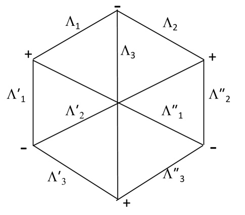
Figure 6.1: Yutsis diagram representing Eq. (6.3). We note that to determine signs at the vertices for some pairs (e.g. $\Lambda_{1}^{\prime},\Lambda_{3}^{\prime}$ one needs to read the 3-$j$ in a cyclic (ring-like) fashion. For instance, with the ordering $\Lambda_{1}^{\prime}\Lambda_{2}^{\prime}\Lambda_{3}^{\prime}$, one should read cyclically as $\Lambda_{1}^{\prime}\Lambda_{2}^{\prime}\Lambda_{3}^{\prime}\Lambda_{1}^{\prime}\ldots$ so that $\Lambda_{3}^{\prime}$ in fact comes before $\Lambda_{1}^{\prime}$. This ordering is obtained by moving clockwise on the Yutsis diagram above, so we assign a $-$ sign at the vertex between $\Lambda_{3}^{\prime}$ and $\Lambda_{1}^{\prime}$.

We find the representation of Eq. (6.3) shown in Fig. 6.1. Comparing with Fig. C.2 or Eq. (B.95) we identify the 9-$j$ symbol

$${\cal Q}^{\Lambda\Lambda^{\prime}\Lambda^{\prime\prime}}={\cal S}^{\Lambda\Lambda^{\prime}\Lambda^{\prime\prime}}=\left\{\begin{array}[]{ccc}{\Lambda_{1}}&{\Lambda^{\prime}_{1}}&{{\Lambda^{\prime\prime}}_{1}}\\ {\Lambda_{2}}&{\Lambda^{\prime}_{2}}&{{\Lambda^{\prime\prime}}_{2}}\\ {\Lambda_{3}}&{\Lambda^{\prime}_{3}}&{{\Lambda^{\prime\prime}}_{3}}\end{array}\right\}.$$ (110)

Inserting this result into Eq. (55), as well as computing ${\cal D}^{\rm P}$ and inserting it also, we find

$${\cal G}^{\Lambda\Lambda^{\prime}\Lambda^{\prime\prime}} =(4\pi)^{-3/2}\left[\prod_{i=1}^{3}\sqrt{(2\Lambda_{i}+1)(2\Lambda^{\prime}_{i}+1)(2\Lambda^{\prime\prime}_{i}+1)}\left(\begin{array}[]{ccc}{\Lambda_{i}}\!&{\Lambda^{\prime}_{i}}\!&{{\Lambda^{\prime\prime}}_{i}}\!\\ {0}\!&{0}\!&{0}\!\\ \end{array}\right)\right]$$ (113)

$$\times\left\{\begin{array}[]{ccc}{\Lambda_{1}}&{\Lambda^{\prime}_{1}}&{{\Lambda^{\prime\prime}}_{1}}\\ {\Lambda_{2}}&{\Lambda^{\prime}_{2}}&{{\Lambda^{\prime\prime}}_{2}}\\ {\Lambda_{3}}&{\Lambda^{\prime}_{3}}&{{\Lambda^{\prime\prime}}_{3}}\end{array}\right\}.$$ (117)

As an example, let us consider ${\cal P}_{110}({\hat{\bf r}}_{1},{\hat{\bf r}}_{2},{\hat{\bf r}}_{3}){\cal P}_{011}({\hat{\bf r}}_{1},{\hat{\bf r}}_{2},{\hat{\bf r}}_{3})$, where we indicate $\Lambda$ in the subscripts by $\Lambda_{1},\Lambda_{2},\Lambda_{3}$. We will use:

$${\cal P}_{110}({\hat{\bf r}}_{1},{\hat{\bf r}}_{2},{\hat{\bf r}}_{3}) = -\sqrt{\frac{3}{(4\pi)^{3}}}\left({\hat{\bf r}}_{1}\cdot{\hat{\bf r}}_{2}\right),$$

$${\cal P}_{011}({\hat{\bf r}}_{1},{\hat{\bf r}}_{2},{\hat{\bf r}}_{3}) = -\sqrt{\frac{3}{(4\pi)^{3}}}\left({\hat{\bf r}}_{2}\cdot{\hat{\bf r}}_{3}\right),$$

$${\cal P}_{121}({\hat{\bf r}}_{1},{\hat{\bf r}}_{2},{\hat{\bf r}}_{3}) = \sqrt{\frac{27}{2(4\pi)^{3}}}\left[({\hat{\bf r}}_{1}\cdot{\hat{\bf r}}_{2})\,({\hat{\bf r}}_{3}\cdot{\hat{\bf r}}_{2})-\frac{1}{3}{\hat{\bf r}}_{1}\cdot{\hat{\bf r}}_{3}\right].$$ (118)

We note that the second line comes from simply interchanging arguments $3\leftrightarrow 1$ in the first line; ${\cal P}_{121}$ similarly comes from interchanging $2\leftrightarrow 3$ in ${\cal P}_{112}$ as given in Appendix A. We now may determine the product

$${\cal P}_{110}({\hat{\bf r}}_{1},{\hat{\bf r}}_{2},{\hat{\bf r}}_{3}){\cal P}_{011}({\hat{\bf r}}_{1},{\hat{\bf r}}_{2},{\hat{\bf r}}_{3})=\frac{3}{(4\pi)^{3}}({\hat{\bf r}}_{1}\cdot{\hat{\bf r}}_{2})\,({\hat{\bf r}}_{2}\cdot{\hat{\bf r}}_{3})$$

$$\qquad=\frac{1}{(4\pi)^{3/2}}\left[\sqrt{\frac{2}{3}}{\cal P}_{121}({\hat{\bf r}}_{1},{\hat{\bf r}}_{2},{\hat{\bf r}}_{3})-\sqrt{\frac{1}{3}}{\cal P}_{101}({\hat{\bf r}}_{1},{\hat{\bf r}}_{2},{\hat{\bf r}}_{3})\right].$$ (119)

We note that ${\cal P}_{101}$ is obtained by interchanging arguments as $1\leftrightarrow 2$ in ${\cal P}_{011}$ of Eq. (118).

We can compare Eq. (119) to our general result Eq. (52) using the values

$${\cal G}^{(110)(011)(121)} = \frac{27\sqrt{5}}{(4\pi)^{3/2}}\left\{\begin{array}[]{ccc}{1}&{1}&{0}\\ {0}&{1}&{1}\\ {1}&{2}&{1}\end{array}\right\}\left(\begin{array}[]{ccc}{1}\!&{1}\!&{0}\!\\ {0}\!&{0}\!&{0}\!\\ \end{array}\right)\left(\begin{array}[]{ccc}{0}\!&{1}\!&{1}\!\\ {0}\!&{0}\!&{0}\!\\ \end{array}\right)\left(\begin{array}[]{ccc}{1}\!&{2}\!&{1}\!\\ {0}\!&{0}\!&{0}\!\\ \end{array}\right)$$ (129)

$$= \frac{27\sqrt{5}}{(4\pi)^{3/2}}\frac{1}{9}\left(-\frac{1}{\sqrt{3}}\right)^{2}\sqrt{\frac{2}{15}}=\frac{1}{(4\pi)^{3/2}}\;\sqrt{\frac{2}{3}}.$$ (130)

and

$${\cal G}^{(110)(011)(101)} = \frac{27}{(4\pi)^{3/2}}\left\{\begin{array}[]{ccc}{1}&{1}&{0}\\ {0}&{1}&{1}\\ {1}&{0}&{1}\end{array}\right\}\left(\begin{array}[]{ccc}{1}\!&{1}\!&{0}\!\\ {0}\!&{0}\!&{0}\!\\ \end{array}\right)\left(\begin{array}[]{ccc}{0}\!&{1}\!&{1}\!\\ {0}\!&{0}\!&{0}\!\\ \end{array}\right)\left(\begin{array}[]{ccc}{1}\!&{0}\!&{1}\!\\ {0}\!&{0}\!&{0}\!\\ \end{array}\right)$$ (140)

$$= \frac{27}{(4\pi)^{3/2}}\frac{1}{9}\left(-\frac{1}{\sqrt{3}}\right)^{3}=\frac{1}{(4\pi)^{3/2}}\left(-\sqrt{\frac{1}{3}}\right).$$ (141)

We have used sympy.physics.wigner to evaluate the 9-$j$ and 3-$j$ symbols above; these can also be computed using a program by A. Stone available through a web interface. We find agreement between the coefficients as given by Eqs. (130) and (141) and as given by Eq. (119).

An example involving parity-odd functions is

$${\cal P}_{111}({\hat{\bf r}}_{1},{\hat{\bf r}}_{2},{\hat{\bf r}}_{3}){\cal P}_{111}({\hat{\bf r}}_{1},{\hat{\bf r}}_{2},{\hat{\bf r}}_{3})=\frac{1}{(4\pi)^{3/2}}\Big{[}\frac{\sqrt{14}}{5}{\cal P}_{222}({\hat{\bf r}}_{1},{\hat{\bf r}}_{2},{\hat{\bf r}}_{3})+$$

$$\qquad+\frac{1}{\sqrt{5}}\left[{\cal P}_{220}({\hat{\bf r}}_{1},{\hat{\bf r}}_{2},{\hat{\bf r}}_{3})+{\cal P}_{202}({\hat{\bf r}}_{1},{\hat{\bf r}}_{2},{\hat{\bf r}}_{3})+{\cal P}_{022}({\hat{\bf r}}_{1},{\hat{\bf r}}_{2},{\hat{\bf r}}_{3})\right]$$

$$\qquad\qquad-{\cal P}_{000}({\hat{\bf r}}_{1},{\hat{\bf r}}_{2},{\hat{\bf r}}_{3})\Big{]}.$$ (142)

The functions used above are listed in Appendix A. We inserted in Eq. (117) $(\Lambda_{1},\Lambda_{2},\Lambda_{3})=(1,1,1)$, $(\Lambda^{\prime}_{1},\Lambda^{\prime}_{2},\Lambda^{\prime}_{3})=(1,1,1)$, and $(\Lambda^{\prime\prime}_{1},\Lambda^{\prime\prime}_{2},\Lambda^{\prime\prime}_{3})=(2,2,2)$ to obtain the ${\cal P}_{222}$ coefficient, $(\Lambda^{\prime\prime}_{1},\Lambda^{\prime\prime}_{2},\Lambda^{\prime\prime}_{3})=(2,2,0)$ to obtain the ${\cal P}_{220}$ coefficient, $(\Lambda^{\prime\prime}_{1},\Lambda^{\prime\prime}_{2},\Lambda^{\prime\prime}_{3})=(2,0,2)$ to obtain the ${\cal P}_{202}$ coefficient, etc. We note that the middle three coefficients must be the same by inspection because of the interchange symmetry of the left-hand side.

6.4 Products of ${\cal P}_{\Lambda}$ for $N=4$

For $N=4$ there are intermediate angular momenta: $\Lambda_{12},\;\Lambda^{\prime}_{12},$ and $\Lambda^{\prime\prime}_{12}$. We recall that the general expansion coefficients are given by Eq. (58), and the phases required for the Yutsis diagram are supplied by the factor $(-1)^{\kappa_{\Lambda}+\kappa_{\Lambda^{\prime}}+\kappa_{\Lambda^{\prime\prime}}}$ in this result, where $\kappa$ is itself defined in Eq. (79). To construct the Yutsis diagram it suffices to examine the upper portions of the 3-$j$ symbols dictated by Eq. (58) since all the various $m_{i}$ are simply summed over. The upper portion written out schematically is:

$$(\Lambda_{1},\Lambda_{2},\Lambda_{12});(\Lambda^{\prime}_{1},\Lambda^{\prime}_{2},\Lambda^{\prime}_{12});({\Lambda^{\prime\prime}}_{1},{\Lambda^{\prime\prime}}_{2},{\Lambda^{\prime\prime}}_{12});$$

$$(\Lambda_{12},\Lambda_{3},\Lambda_{4});(\Lambda^{\prime}_{12},\Lambda^{\prime}_{3},\Lambda^{\prime}_{4})({\Lambda^{\prime\prime}}_{12},{\Lambda^{\prime\prime}}_{3},{\Lambda^{\prime\prime}}_{4});$$

$$(\Lambda_{1},\Lambda^{\prime}_{1},{\Lambda^{\prime\prime}}_{1});(\Lambda_{2},\Lambda^{\prime}_{2},{\Lambda^{\prime\prime}}_{2});(\Lambda_{3},\Lambda^{\prime}_{3},{\Lambda^{\prime\prime}}_{3});(\Lambda_{4},\Lambda^{\prime}_{4},{\Lambda^{\prime\prime}}_{4}).$$ (143)

From this we derive the Yutsis diagram in Fig. 6.2.

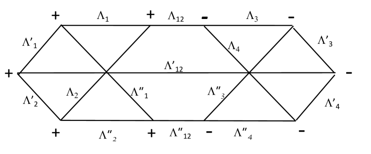
Figure 6.2: Yutsis diagram describing the coefficient of ${\cal P}_{\Lambda^{\prime\prime}}$ in the product of the four-point functions ${\cal P}_{\Lambda}$ and ${\cal P}_{\Lambda^{\prime}}$.

The plus and minus signs are determined by the order of the $j$ values in the various 3-$j$ symbols. To reach the canonical forms we change some of the signs to produce Fig. 6.3. At each vertex where the sign is reversed a factor $(-1)^{j_{a}+j_{b}+j_{c}}$ is induced, where $j_{a},j_{b}$ and $j_{c}$ are the angular momenta in the associated 3-$j$ symbol. In our set of flips, the overall factor is $-1$ raised to the sum of the $\Lambda_{i}$, the $\Lambda^{\prime}_{i}$, the ${\Lambda^{\prime\prime}}_{i}$, and $2(\Lambda_{12}+\Lambda^{\prime}_{12}+{\Lambda^{\prime\prime}}_{12})$. This sum is even, so the overall factor is unity.

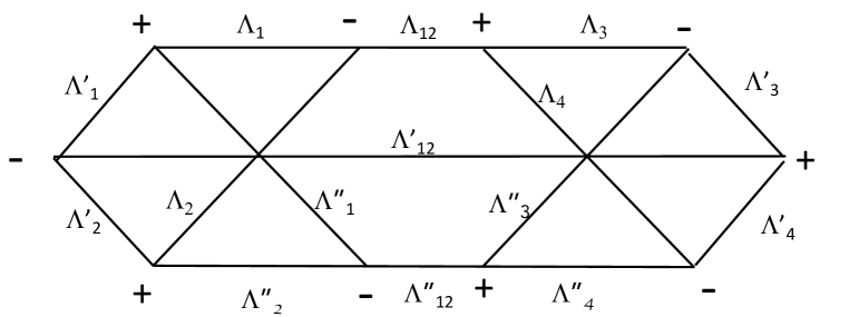
Figure 6.3: Yutsis diagram describing the coefficient of ${\cal P}_{\Lambda^{\prime\prime}}$ in the product of the four-point functions ${\cal P}_{\Lambda}$ and ${\cal P}_{\Lambda^{\prime}}$, but with the factors associated with some vertices changed to create the canonical alternating signs at the vertices.

Yutsis et al. (1962) show that any diagram that can be separated into two disconnected pieces by cutting just three lines is a product of two simpler factors. This is a consequence of their theorem (see Appendix D) that a product $F_{(j_{1},m_{1}),(j_{2},m_{2}),(j_{3},m_{3})}$ of 3-$j$ symbols with three unsummed $j,m$ columns, $(j_{1},m_{1}),(j_{2},m_{2}),(j_{3},m_{3})$, is necessarily proportional to a 3-$j$ symbol

$$F_{(j_{1},m_{1}),(j_{2},m_{2}),(j_{3},m_{3})}=\left(\begin{array}[]{ccc}{j_{1}}\!&{j_{2}}\!&{j_{3}}\!\\ {m_{1}}\!&{m_{2}}\!&{m_{3}}\!\\ \end{array}\right)F.$$ (144)

The factored diagram stemming from Fig. 6.3 is shown in Fig. 6.4.

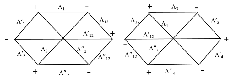
Figure 6.4: Yutsis diagram showing the result of cutting the three lines in Fig. 6.3 corresponding to $\Lambda_{12},\Lambda^{\prime}_{12},$ and $\Lambda^{\prime\prime}_{12}$.

To compute ${\cal G}^{\Lambda\Lambda^{\prime}\Lambda^{\prime\prime}}$ using Eq. (55), we need ${\cal Q}^{\Lambda\Lambda^{\prime}\Lambda^{\prime\prime}}$, which in turn requires ${\cal S}^{\Lambda\Lambda^{\prime}\Lambda^{\prime\prime}}$ by Eq. (80). Comparing the two diagrams in Fig. 6.4 to that for the canonical 9-j symbol, given in Fig. C.2, we find that

$${\cal S}^{\Lambda\Lambda^{\prime}\Lambda^{\prime\prime}} = \left\{\begin{array}[]{ccc}{\Lambda_{1}}&{\Lambda_{12}}&{\Lambda_{2}}\\ {\Lambda^{\prime}_{1}}&{\Lambda^{\prime}_{12}}&{\Lambda^{\prime}_{2}}\\ {{\Lambda^{\prime\prime}}_{1}}&{\Lambda^{\prime\prime}_{12}}&{{\Lambda^{\prime\prime}}_{2}}\end{array}\right\}\left\{\begin{array}[]{ccc}{\Lambda_{3}}&{\Lambda_{12}}&{\Lambda_{4}}\\ {\Lambda^{\prime}_{3}}&{\Lambda^{\prime}_{12}}&{\Lambda^{\prime}_{4}}\\ {{\Lambda^{\prime\prime}}_{3}}&{{\Lambda^{\prime\prime}}_{12}}&{{\Lambda^{\prime\prime}}_{4}}\end{array}\right\}$$ (151)

$$= \left\{\begin{array}[]{ccc}{\Lambda_{1}}&{\Lambda_{2}}&{\Lambda_{12}}\\ {\Lambda^{\prime}_{1}}&{\Lambda^{\prime}_{2}}&{\Lambda^{\prime}_{12}}\\ {{\Lambda^{\prime\prime}}_{1}}&{{\Lambda^{\prime\prime}}_{2}}&{{\Lambda^{\prime\prime}}_{12}}\end{array}\right\}\left\{\begin{array}[]{ccc}{\Lambda_{12}}&{\Lambda_{3}}&{\Lambda_{4}}\\ {\Lambda^{\prime}_{12}}&{\Lambda^{\prime}_{3}}&{\Lambda^{\prime}_{4}}\\ {{\Lambda^{\prime\prime}}_{12}}&{{\Lambda^{\prime\prime}}_{3}}&{{\Lambda^{\prime\prime}}_{4}}\end{array}\right\}.$$ (158)

We note that we chose $j_{1}=\Lambda_{1}$, $j_{2}=\Lambda_{12}$ when comparing the left-hand Yutsis diagram of Fig. 6.4 to Fig. C.2. For the right-hand Yutsis diagram of Fig. 6.4, we chose $j_{1}=\Lambda_{3}$, $j_{2}=\Lambda_{12}$ when comparing to Fig. C.2; this was motivated by wanting to preserve mirror symmetry regarding the role of $\Lambda_{12}$ between the two halves of Fig. 6.4. We note that the signs in Fig. 6.4 flip under this symmetry, as is indeed seen in the diagrams. We note also that the rearrangement of the columns going from the first to the second line above leaves the overall sign unchanged. The coefficient we seek is, using Eqs. (55), (80), and (81):

$${\cal G}^{\Lambda\Lambda^{\prime}\Lambda^{\prime\prime}} =\sqrt{(2\Lambda_{12}+1)(2\Lambda^{\prime}_{12}+1)(2{\Lambda^{\prime\prime}}_{12}+1)}$$

$$\times(4\pi)^{-2}\prod_{i=1}^{4}\sqrt{(2\Lambda_{i}+1)(2\Lambda^{\prime}_{i}+1)(2{\Lambda^{\prime\prime}}_{i}+1)}\left(\begin{array}[]{ccc}{\Lambda_{i}}\!&{\Lambda^{\prime}_{i}}\!&{{\Lambda^{\prime\prime}}_{i}}\!\\ {0}\!&{0}\!&{0}\!\\ \end{array}\right)$$ (161)

$$\times\left\{\begin{array}[]{ccc}{\Lambda_{1}}&{\Lambda_{2}}&{\Lambda_{12}}\\ {\Lambda^{\prime}_{1}}&{\Lambda^{\prime}_{2}}&{\Lambda^{\prime}_{12}}\\ {{\Lambda^{\prime\prime}}_{1}}&{{\Lambda^{\prime\prime}}_{2}}&{{\Lambda^{\prime\prime}}_{12}}\end{array}\right\}\left\{\begin{array}[]{ccc}{\Lambda_{12}}&{\Lambda_{3}}&{\Lambda_{4}}\\ {\Lambda^{\prime}_{12}}&{\Lambda^{\prime}_{3}}&{\Lambda^{\prime}_{4}}\\ {{\Lambda^{\prime\prime}}_{12}}&{{\Lambda^{\prime\prime}}_{3}}&{{\Lambda^{\prime\prime}}_{4}}\end{array}\right\}.$$ (168)

As an example, we calculate ${\cal P}_{11(1)11}{\cal P}_{10(1)01}$. By applying the triangle rule on angular momentum addition, we see that the possible values for ${\Lambda^{\prime\prime}}_{i}$ are ${\Lambda^{\prime\prime}}_{1}=0,1,2$, ${\Lambda^{\prime\prime}}_{2}=1$, ${\Lambda^{\prime\prime}}_{3}=1$, ${\Lambda^{\prime\prime}}_{4}=0,1,2$ and ${\Lambda^{\prime\prime}}_{12}=0,1,2$. Algebraic manipulation of the Cartesian forms in Eq. (A.3) shows

$${\cal P}_{11(1)11}({\hat{\bf r}}_{1},{\hat{\bf r}}_{2},{\hat{\bf r}}_{3},{\hat{\bf r}}_{4}){\cal P}_{10(1)01}({\hat{\bf r}}_{1},{\hat{\bf r}}_{2},{\hat{\bf r}}_{3},{\hat{\bf r}}_{4})$$

$$\quad=\frac{1}{(4\pi)^{2}}\bigg{[}\frac{3}{2\sqrt{5}}{\cal P}_{21(2)12}({\hat{\bf r}}_{1},{\hat{\bf r}}_{2},{\hat{\bf r}}_{3},{\hat{\bf r}}_{4})-\frac{1}{2\sqrt{3}}{\cal P}_{21(1)12}({\hat{\bf r}}_{1},{\hat{\bf r}}_{2},{\hat{\bf r}}_{3},{\hat{\bf r}}_{4})$$

$$\qquad\qquad-\frac{1}{\sqrt{6}}\left[{\cal P}_{21(1)10}({\hat{\bf r}}_{1},{\hat{\bf r}}_{2},{\hat{\bf r}}_{3},{\hat{\bf r}}_{4})+{\cal P}_{01(1)12}({\hat{\bf r}}_{1},{\hat{\bf r}}_{2},{\hat{\bf r}}_{3},{\hat{\bf r}}_{4})\right]$$

$$\qquad\qquad\qquad-\frac{1}{\sqrt{3}}{\cal P}_{01(1)10}({\hat{\bf r}}_{1},{\hat{\bf r}}_{2},{\hat{\bf r}}_{3},{\hat{\bf r}}_{4})\bigg{]}.$$ (169)

The same result is obtained from Eq. (168), which can be evaluated conveniently with the python package sympy.physics.wigner. We note that mapping ${\hat{\bf r}}_{4}\to{\hat{\bf r}}_{1}$ converts ${\cal P}_{21(1)10}$ to ${\cal P}_{01(1)12}$, and given that the Universe is insensitive to our choice of labels, this implies that these two functions’ coefficients must be the same in our expansion above.

As a second example we consider a product with a parity-odd factor. Using Eq. (168) we obtain:

$${\cal P}_{11(1)10}({\hat{\bf r}}_{1},{\hat{\bf r}}_{2},{\hat{\bf r}}_{3},{\hat{\bf r}}_{4}){\cal P}_{10(1)01}({\hat{\bf r}}_{1},{\hat{\bf r}}_{2},{\hat{\bf r}}_{3},{\hat{\bf r}}_{4})$$

$$\qquad=\frac{1}{(4\pi)^{2}}\bigg{[}\sqrt{\frac{1}{2}}{\cal P}_{21(2)11}({\hat{\bf r}}_{1},{\hat{\bf r}}_{2},{\hat{\bf r}}_{3},{\hat{\bf r}}_{4})-\sqrt{\frac{1}{6}}{\cal P}_{21(1)11}({\hat{\bf r}}_{1},{\hat{\bf r}}_{2},{\hat{\bf r}}_{3},{\hat{\bf r}}_{4})$$

$$\qquad\qquad-\sqrt{\frac{1}{3}}{\cal P}_{01(1)11}({\hat{\bf r}}_{1},{\hat{\bf r}}_{2},{\hat{\bf r}}_{3},{\hat{\bf r}}_{4})\bigg{]}.$$ (170)

6.5 Products of ${\cal P}_{\Lambda}$ for $N=5$

For $N=5$ there are two sets of intermediate angular momenta: $\Lambda_{12},\Lambda^{\prime}_{12},{\Lambda^{\prime\prime}}_{12}$ and $\Lambda_{123},\Lambda^{\prime}_{123},{\Lambda^{\prime\prime}}_{123}$. The phases required for the Yutsis diagram are supplied by the factor $(-1)^{\kappa_{\Lambda}+\kappa_{\Lambda^{\prime}}+\kappa_{\Lambda^{\prime\prime}}}$, itself defined in Eq. (79). To construct the Yutsis diagram it suffices to examine the upper portions of the 3-$j$ symbols in $\mathcal{G}$ (Eq. 55) and specifically its factor $\mathcal{Q}$ as defined in Eq. (58):

$$(\Lambda_{1},\Lambda_{2},\Lambda_{12});(\Lambda^{\prime}_{1},\Lambda^{\prime}_{2},\Lambda^{\prime}_{12});({\Lambda^{\prime\prime}}_{1},{\Lambda^{\prime\prime}}_{2},{\Lambda^{\prime\prime}}_{12});$$ (171)

$$(\Lambda_{12},\Lambda_{3},\Lambda_{123});(\Lambda^{\prime}_{12},\Lambda^{\prime}_{3},\Lambda^{\prime}_{123});({\Lambda^{\prime\prime}}_{12},{\Lambda^{\prime\prime}}_{3},{\Lambda^{\prime\prime}}_{123});$$

$$(\Lambda_{123},\Lambda_{4},\Lambda_{5});(\Lambda^{\prime}_{123},\Lambda^{\prime}_{4},\Lambda^{\prime}_{5});({\Lambda^{\prime\prime}}_{123},{\Lambda^{\prime\prime}}_{4},{\Lambda^{\prime\prime}}_{5});$$

$$(\Lambda_{1},\Lambda^{\prime}_{1},{\Lambda^{\prime\prime}}_{1});(\Lambda_{2},\Lambda^{\prime}_{2},{\Lambda^{\prime\prime}}_{2});(\Lambda_{3},\Lambda^{\prime}_{3},{\Lambda^{\prime\prime}}_{3});(\Lambda_{4},\Lambda^{\prime}_{4},{\Lambda^{\prime\prime}}_{4});(\Lambda_{5},\Lambda^{\prime}_{5},{\Lambda^{\prime\prime}}_{5}).$$

From this we derive the diagram in Fig. 6.5.

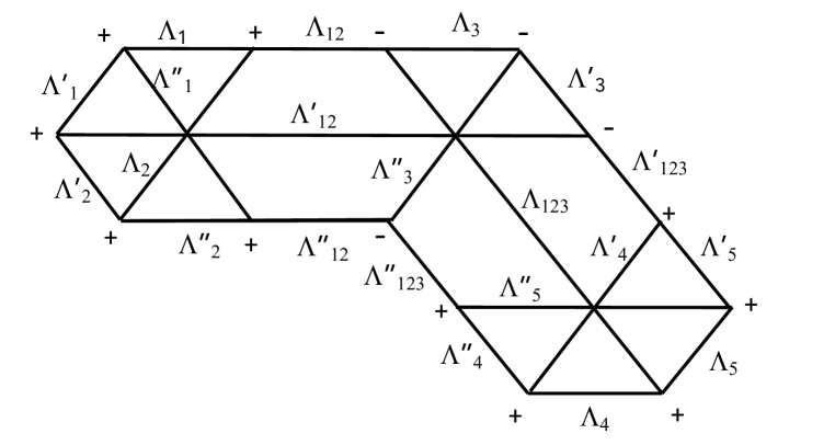
Figure 6.5: Yutsis diagram describing the coefficient of ${\cal P}_{\Lambda^{\prime\prime}}$ in the product of the five-point functions ${\cal P}_{\Lambda}$ and ${\cal P}_{\Lambda^{\prime}}$; the diagram is derived from Eq. (171). We will cut it across the set of three lines representing the intermediate momenta $\Lambda_{12},\Lambda^{\prime}_{12},\Lambda_{12}^{\prime\prime}$ and also across the set of three lines representing $\Lambda_{123},\Lambda^{\prime}_{123},\Lambda_{123}^{\prime\prime}$ to obtain Fig. 6.6.

This diagram can be divided into three separate pieces by cutting through three lines in two different places. We cut through the lines representing $\Lambda_{12},\Lambda^{\prime}_{12}$ and $\Lambda^{\prime\prime}_{12}$ and also the lines representing $\Lambda_{132},\Lambda^{\prime}_{123},\Lambda^{\prime\prime}_{123}$. Notably, these are the lines representing all of the intermediate momenta. The result is shown in Fig. 6.6.

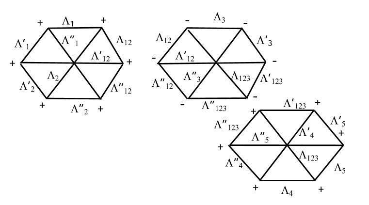
Figure 6.6: Yutsis diagram Fig. 6.5 factored by cutting that diagram at the lines representing the intermediate momenta, as detailed in the caption for Fig. 6.5.

To bring the three separate diagrams to canonical form for 9-$j$ symbols introduces a factor $(-1)^{\sum_{i=1}^{5}(\Lambda_{i}+\Lambda^{\prime}_{i}+{\Lambda^{\prime\prime}}_{i})}$, which is simply $+1$ by consideration of parity.

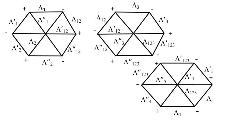
Figure 6.7: The Yutsis diagram for $N=5$ (Fig. 6.5) after splitting (Fig. 6.6) and now with canonical signs at the vertices (compare with Fig. 6.6).

Comparing with Fig. C.2 showing the canonical diagram for a 9-$j$ symbol we find that the three diagrams give directly

$${\cal S}^{\Lambda\Lambda^{\prime}\Lambda^{\prime\prime}}$$ (172)

$$=\left\{\begin{array}[]{ccc}{\Lambda_{1}}&{\Lambda_{12}}&{\Lambda_{2}}\\ {\Lambda^{\prime}_{1}}&{\Lambda^{\prime}_{12}}&{\Lambda^{\prime}_{2}}\\ {{\Lambda^{\prime\prime}}_{1}}&{{\Lambda^{\prime\prime}}_{12}}&{{\Lambda^{\prime\prime}}_{2}}\end{array}\right\}\left\{\begin{array}[]{ccc}{\Lambda_{3}}&{\Lambda_{12}}&{\Lambda_{123}}\\ {\Lambda^{\prime}_{3}}&{\Lambda^{\prime}_{12}}&{\Lambda^{\prime}_{123}}\\ {{\Lambda^{\prime\prime}}_{3}}&{{\Lambda^{\prime\prime}}_{12}}&{{\Lambda^{\prime\prime}}_{123}}\end{array}\right\}\left\{\begin{array}[]{ccc}{\Lambda_{5}}&{\Lambda_{4}}&{\Lambda_{123}}\\ {\Lambda^{\prime}_{5}}&{\Lambda^{\prime}_{4}}&{\Lambda^{\prime}_{123}}\\ {{\Lambda^{\prime\prime}}_{5}}&{{\Lambda^{\prime\prime}}_{4}}&{{\Lambda^{\prime\prime}}_{123}}\end{array}\right\}$$ (182)

$$=\left\{\begin{array}[]{ccc}{\Lambda_{1}}&{\Lambda_{2}}&{\Lambda_{12}}\\ {\Lambda^{\prime}_{1}}&{\Lambda^{\prime}_{2}}&{\Lambda^{\prime}_{12}}\\ {{\Lambda^{\prime\prime}}_{1}}&{{\Lambda^{\prime\prime}}_{2}}&{{\Lambda^{\prime\prime}}_{12}}\end{array}\right\}\left\{\begin{array}[]{ccc}{\Lambda_{12}}&{\Lambda_{3}}&{\Lambda_{123}}\\ {\Lambda^{\prime}_{12}}&{\Lambda^{\prime}_{3}}&{\Lambda^{\prime}_{123}}\\ {{\Lambda^{\prime\prime}}_{12}}&{{\Lambda^{\prime\prime}}_{3}}&{{\Lambda^{\prime\prime}}_{123}}\end{array}\right\}\left\{\begin{array}[]{ccc}{\Lambda_{123}}&{\Lambda_{4}}&{\Lambda_{5}}\\ {\Lambda^{\prime}_{123}}&{\Lambda^{\prime}_{4}}&{\Lambda^{\prime}_{5}}\\ {{\Lambda^{\prime\prime}}_{123}}&{{\Lambda^{\prime\prime}}_{4}}&{{\Lambda^{\prime\prime}}_{5}}\end{array}\right\}.$$ (192)

We recall that ${\cal S}^{\Lambda\Lambda^{\prime}\Lambda^{\prime\prime}}$ is one of the two factors in $\mathcal{Q}$, which in turn enters $\mathcal{G}$, the overall expansion coefficient for turning a product of two isotropic functions into a sum over single ones. We recall further that ${\cal S}^{\Lambda\Lambda^{\prime}\Lambda^{\prime\prime}}$ is defined through Eqs. (58 ) and (80). When comparing Fig. 6.7 with Fig. C.2 we identify for the first diagram $j_{1}=\Lambda_{1},j_{2}=\Lambda_{12}$, etc. For the second diagram, we identify $j_{1}=\Lambda_{3},j_{2}=\Lambda_{12}$, etc. For the third diagram, we identify $j_{1}=\Lambda_{5},j_{2}=\Lambda_{4}$, etc. These choices give the 9-$j$ symbols in the first line above. We have made them with the same reasoning about mirror symmetry about the points where the diagrams separated as discussed below Eq. (151). We can then use the symmetries of the 9-$j$ symbol (described in Appendix B, §B.3) to interchange two columns in each of the 9-$j$ symbols. Because parity requires ${\cal E}(\Lambda){\cal E}(\Lambda^{\prime}){\cal E}(\Lambda^{\prime\prime})=1$, this does not change the overall sign.

The full coefficient we seek is then

$${\cal G}_{\Lambda\Lambda^{\prime}}^{\Lambda^{\prime\prime}} = \sqrt{(2\Lambda_{12}+1)(2\Lambda^{\prime}_{12}+1)(2{\Lambda^{\prime\prime}}_{12}+1)(2\Lambda_{123}+1)(2\Lambda^{\prime}_{123}+1)(2{\Lambda^{\prime\prime}}_{123}+1)}$$ (205)

$$\times(4\pi)^{-5/2}\left[\prod_{i=1}^{5}\sqrt{(2\Lambda_{i}+1)(2\Lambda^{\prime}_{i}+1)(2{\Lambda^{\prime\prime}}_{i}+1)}\left(\begin{array}[]{ccc}{\Lambda_{i}}\!&{\Lambda^{\prime}_{i}}\!&{{\Lambda^{\prime\prime}}_{i}}\!\\ {0}\!&{0}\!&{0}\!\\ \end{array}\right)\right]$$

$$\quad\times\left\{\begin{array}[]{ccc}{\Lambda_{1}}&{\Lambda_{2}}&{\Lambda_{12}}\\ {\Lambda^{\prime}_{1}}&{\Lambda^{\prime}_{2}}&{\Lambda^{\prime}_{12}}\\ {{\Lambda^{\prime\prime}}_{1}}&{{\Lambda^{\prime\prime}}_{2}}&{{\Lambda^{\prime\prime}}_{12}}\end{array}\right\}\left\{\begin{array}[]{ccc}{\Lambda_{12}}&{\Lambda_{3}}&{\Lambda_{123}}\\ {\Lambda^{\prime}_{12}}&{\Lambda^{\prime}_{3}}&{\Lambda^{\prime}_{123}}\\ {{\Lambda^{\prime\prime}}_{12}}&{{\Lambda^{\prime\prime}}_{3}}&{{\Lambda^{\prime\prime}}_{123}}\end{array}\right\}\left\{\begin{array}[]{ccc}{\Lambda_{123}}&{\Lambda_{4}}&{\Lambda_{5}}\\ {\Lambda^{\prime}_{123}}&{\Lambda^{\prime}_{4}}&{\Lambda^{\prime}_{5}}\\ {{\Lambda^{\prime\prime}}_{123}}&{{\Lambda^{\prime\prime}}_{4}}&{{\Lambda^{\prime\prime}}_{5}}\end{array}\right\}.$$

7 Reordering of arguments in ${\cal P}_{\Lambda}$

The ${\cal P}_{\Lambda}({\hat{\bf r}}_{1},\ldots,{\hat{\bf r}}_{N})$ provide an orthonormal basis for expanding isotropic functions of ${\hat{\bf r}}_{i}$, $i=1,\ldots,N$. The definition of the canonical order $i=1,\ldots,N$ must be supplied, for example by an ordering of the $r_{i}\equiv|{\bf r}_{i}|$. A computation in terms of the ${\cal P}_{\Lambda}$ can, however, lead to an expression in terms of a ${\cal P}_{\Lambda}$ whose arguments are not in the canonical order. Including these additional isotropic functions would result in an over-complete basis, which would prevent identification of physically significant quantities. So motivated, we consider a reordering of ${\hat{\bf r}}_{1},\ldots,{\hat{\bf r}}_{N}$ as ${\hat{\bf r}}_{F1},\ldots,{\hat{\bf r}}_{FN}$ and our ${\cal P}_{\Lambda}$ evaluated at those arguments, as ${\cal P}_{\Lambda}({\hat{\bf r}}_{F1},\ldots,,{\hat{\bf r}}_{FN})$. Since the canonically-ordered ${\cal P}_{\Lambda}$ are a complete basis, the non-canonically ordered function must be expressible in terms of a sum of canonically ordered ones, each weighted by a coefficient ${\cal B}^{F}_{\Lambda,\Lambda^{\prime}}$:

$${\cal P}_{\Lambda}({\hat{\bf r}}_{F1},\ldots,{\hat{\bf r}}_{FN})=\sum_{\Lambda^{\prime}}{\cal B}^{F}_{\Lambda,\Lambda^{\prime}}{\cal P}_{\Lambda^{\prime}}({\hat{\bf r}}_{1},\ldots,{\hat{\bf r}}_{N}).$$ (206)

Using Eq. (5), orthogonality then determines that

$${\cal B}^{F}_{\Lambda,\Lambda^{\prime}} = \int d{\hat{\bf R}}\,{\cal P}_{\Lambda}({\hat{\bf r}}_{F1},\ldots,{\hat{\bf r}}_{FN}){\cal P}^{*}_{\Lambda^{\prime}}({\hat{\bf r}}_{1},\ldots,{\hat{\bf r}}_{N})$$ (207)

$$= \int d{\hat{\bf R}}\,\sum_{M_{i},M^{\prime}_{j}}{\cal C}^{\Lambda}_{M}\prod_{i=1}^{N}Y_{\Lambda_{i}M_{i}}({\hat{\bf r}}_{Fi})\;{\cal C}^{\Lambda^{\prime}}_{M^{\prime}}\prod_{j=1}^{N}Y^{*}_{\Lambda^{\prime}_{j}M^{\prime}_{j}}({\hat{\bf r}}_{j})$$

where $d{\hat{\bf R}}\,=d{\hat{\bf r}}\,_{1}\cdots d{\hat{\bf r}}\,_{N}$ and we used the definition Eq. (4) of ${\cal P}$.

Now, $F$ takes $i$ to some value within the original set $1,\ldots,N$. Hence $\Lambda_{1},M_{1}$ now goes with an argument $\hat{\bf r}_{F1}$, etc. We integrate a spherical harmonic of this argument against the conjugate harmonic with the same argument, so from the transformation of e.g. $\hat{\bf r}_{1}$ we have (pulling out from Eq. (207) the $j=F1$ piece)

$$\int d\hat{\bf r}_{F1}\;Y_{\Lambda_{1}M_{1}}(\hat{\bf r}_{F1})Y^{*}_{\Lambda^{\prime}_{F1}M^{\prime}_{F1}}(\hat{\bf r}_{F1}),$$ (208)

and similarly for the transformations of the other $\hat{\bf r}_{i}$.

By orthogonality of the spherical harmonics, we thus see that the integral in Eq. (207) will vanish unless $\Lambda_{1}=\Lambda^{\prime}_{F1}$, and the same argument applies to $\Lambda_{2}=\Lambda^{\prime}_{F2}$, etc. Thus overall we conclude that ${\cal B}^{F}_{\Lambda,\Lambda^{\prime}}$ must include a factor of $\delta^{{\rm K}}_{\Lambda_{1}\Lambda^{\prime}_{F1}}\cdots\delta^{{\rm K}}_{\Lambda_{N}\Lambda^{\prime}_{FN}}$.

The notation simplifies if we use the inverse permutation $G=F^{-1}$. When we use $G$, the Kronecker delta factor derived above becomes $\prod_{i=1}^{N}\delta^{{\rm K}}_{\Lambda^{\prime}_{i}\Lambda_{Gi}}$. We note that the Kronecker deltas act only on the primary momenta, not the intermediate ones, so primed intermediate momenta remain in the calculation. Performing all of the angular integrals in Eq. (207) and then applying the resulting Kronecker deltas to the $primary$ primed momenta, we obtain

$${\cal B}^{F=G^{-1}}_{\Lambda,\Lambda^{\prime}}=\sum_{M_{i}}{\cal C}^{(\Lambda_{1},\Lambda_{2},\Lambda_{12},\ldots\Lambda_{N})}_{(M_{1},M_{2},\ldots M_{N})}{\cal C}^{(\Lambda_{G1},\Lambda_{G2},\Lambda^{\prime}_{12},\ldots\Lambda_{GN})}_{(M_{G1},M_{G2},\ldots M_{GN})}\prod_{i=1}^{N}\delta^{{\rm K}}_{\Lambda^{\prime}_{i}\Lambda_{Gi}}.$$ (209)

We note that the permutation $F$ or $G$ does not appear explicitly in the intermediate momenta $\Lambda_{12},\Lambda^{\prime}_{12}$, etc. Their values are specified initially and are not altered by the permutation. Though we have applied the Kronecker delta factor to the second ${\cal C}$, we still need to include it on the righthand side to specify the values of the $\Lambda^{\prime}_{i}$.

Now, given $\Lambda=\Lambda_{1},\Lambda_{2},\Lambda_{12},\ldots,\Lambda_{N}$ and the permutation $F$, our task is to find the coefficients ${\cal B}^{F}_{\Lambda,\Lambda^{\prime}}$, for the (fixed) values of the intermediate $\Lambda^{\prime}_{12}$, etc.

Re-expressing Eq. (209) using 3-$j$ symbols as in Eq. (19) we find

$${\cal B}^{F=G^{-1}}_{\Lambda,\Lambda^{\prime}} = {\cal E}(\Lambda^{\prime})\sum_{M_{i}}{\cal C}^{(\Lambda_{1},\Lambda_{2},\Lambda_{12},\ldots\Lambda_{N})}_{(M_{1},M_{2},\ldots M_{N})}{\cal C}^{(\Lambda_{G1},\Lambda_{G2},\Lambda^{\prime}_{12},\ldots\Lambda_{GN})}_{(-M_{G1},-M_{G2},\ldots-M_{GN})}\prod_{i=1}^{N}\delta^{{\rm K}}_{\Lambda^{\prime}_{i}\Lambda_{Gi}}$$ (225)

$$= {\cal E}(\Lambda^{\prime})\prod_{i=1}^{N}\delta^{{\rm K}}_{\Lambda^{\prime}_{i}\Lambda_{Gi}}\sum_{M_{i},M_{12}\ldots M^{\prime}_{12}\ldots}(-1)^{(\Lambda_{12}-M_{12}+\ldots)}(-1)^{(\Lambda^{\prime}_{12}-M^{\prime}_{12}+\ldots)}$$

$$\qquad\times\sqrt{2\Lambda_{12}+1}\sqrt{2\Lambda^{\prime}_{12}+1}\cdots\sqrt{2\Lambda_{12\ldots N-2}+1}\sqrt{2\Lambda^{\prime}_{12\ldots N-2}+1}$$

$$\qquad\times\left(\begin{array}[]{ccc}{\Lambda_{1}}\!&{\Lambda_{2}}\!&{\Lambda_{12}}\!\\ {M_{1}}\!&{M_{2}}\!&{-M_{12}}\!\\ \end{array}\right)\left(\begin{array}[]{ccc}{\Lambda_{12}}\!&{\Lambda_{3}}\!&{\Lambda_{123}}\!\\ {M_{12}}\!&{M_{3}}\!&{-M_{123}}\!\\ \end{array}\right)\ldots$$

$$\qquad\qquad\qquad\qquad\qquad\qquad\times\left(\begin{array}[]{ccc}{\Lambda_{12\ldots N-2}}\!&{\Lambda_{N-1}}\!&{\Lambda_{N}}\!\\ {M_{12\ldots N-2}}\!&{M_{N-1}}\!&{M_{N}}\!\\ \end{array}\right)$$

$$\qquad\times\left(\begin{array}[]{ccc}{\Lambda_{G1}}\!&{\Lambda_{G2}}\!&{\Lambda^{\prime}_{12}}\!\\ {-M_{G1}}\!&{-M_{G2}}\!&{M^{\prime}_{12}}\!\\ \end{array}\right)\left(\begin{array}[]{ccc}{\Lambda^{\prime}_{12}}\!&{\Lambda_{G3}}\!&{\Lambda^{\prime}_{123}}\!\\ {-M^{\prime}_{12}}\!&{-M_{G3}}\!&{M^{\prime}_{123}}\!\\ \end{array}\right)\ldots$$

$$\qquad\qquad\qquad\qquad\qquad\qquad\times\left(\begin{array}[]{ccc}{\Lambda^{\prime}_{12\ldots N-2}}\!&{\Lambda_{G(N-1)}}\!&{\Lambda^{\prime}_{GN}}\!\\ {-M^{\prime}_{12\ldots N-2}}\!&{-M_{G(N-1)}}\!&{-M_{GN}}\!\\ \end{array}\right).$$

The factors ${\cal E}(\Lambda^{\prime})={\cal E}(\Lambda)$ and $(-1)^{(\Lambda_{12}-M_{12}+\ldots\Lambda^{\prime}_{12}-M^{\prime}_{12}+\ldots)}$ are just what is required to make the product of the 3-$j$ symbols describable with Yutsis diagrams.

We now discuss some very simple limits to gain intuition about the behavior of ${\cal B}$. First, consider the case where the permutation $F$ leaves alone “1” and “2”, i.e. $G1=1$ and $G2=2$. We may then use the orthogonality relation on the 3-$j$ symbols (B.16), which we rewrite here with the relevant angular momenta filled in for clarity:

$$\sum_{M_{1},M_{2}}\left(\begin{array}[]{ccc}{\Lambda_{1}}\!&{\Lambda_{2}}\!&{\Lambda_{12}}\!\\ {M_{1}}\!&{M_{2}}\!&{-M_{12}}\!\\ \end{array}\right)\left(\begin{array}[]{ccc}{\Lambda_{1}}\!&{\Lambda_{2}}\!&{\Lambda^{\prime}_{12}}\!\\ {-M_{1}}\!&{-M_{2}}\!&{M^{\prime}_{12}}\!\\ \end{array}\right)$$ (230)

$$\qquad=\frac{\delta^{{\rm K}}_{\Lambda_{12}\Lambda^{\prime}_{12}}\delta^{{\rm K}}_{M_{12}M^{\prime}_{12}}}{2\Lambda_{12}+1}(-1)^{\Lambda_{1}+\Lambda_{2}+\Lambda_{12}}.$$

Inserting this in Eq. (225) we find

$${\cal B}^{F=G^{-1}}_{\Lambda,\Lambda^{\prime}}={\cal E}(\Lambda^{\prime})\delta^{{\rm K}}_{\Lambda_{12},\Lambda^{\prime}_{12}}\prod_{i=1}^{N}\delta^{{\rm K}}_{\Lambda^{\prime}_{i}\Lambda_{Gi}}\sum_{M_{12},M_{3}\ldots,\atop M_{123}\ldots M^{\prime}_{123}\ldots}(-1)^{\Lambda_{1}+\Lambda_{2}+\Lambda_{12}}$$ (231)

$$\times(-1)^{(\Lambda_{123}-M_{123}+\Lambda^{\prime}_{123}-M^{\prime}_{123}+\ldots)}\times\sqrt{2\Lambda_{123}+1}\sqrt{2\Lambda^{\prime}_{123}+1}$$

$$\times\left(\begin{array}[]{ccc}{\Lambda_{12}}\!&{\Lambda_{3}}\!&{\Lambda_{123}}\!\\ {M_{12}}\!&{M_{3}}\!&{-M_{123}}\!\\ \end{array}\right)\cdots\left(\begin{array}[]{ccc}{\Lambda_{12\ldots N-2}}\!&{\Lambda_{N-1}}\!&{\Lambda_{N}}\!\\ {M_{12\ldots N-2}}\!&{M_{N-1}}\!&{M_{N}}\!\\ \end{array}\right)$$ (236)

$$\times\left(\begin{array}[]{ccc}{\Lambda_{12}}\!&{\Lambda_{G3}}\!&{\Lambda^{\prime}_{123}}\!\\ {-M_{12}}\!&{-M_{G3}}\!&{M^{\prime}_{123}}\!\\ \end{array}\right)\cdots\left(\begin{array}[]{ccc}{\Lambda^{\prime}_{12\ldots N-2}}\!&{\Lambda_{G(N-1)}}\!&{\Lambda^{\prime}_{GN}}\!\\ {-M^{\prime}_{12\ldots N-2}}\!&{-M_{G(N-1)}}\!&{-M_{GN}}\!\\ \end{array}\right).$$ (241)

Now specializing further to the case where $F$ is the identity permutation, so that $Gi=i$, we recover

$${\cal B}^{F}_{\Lambda\Lambda^{\prime}}=\delta^{{\rm K}}_{\Lambda_{12}\Lambda^{\prime}_{12}}\delta^{{\rm K}}_{\Lambda_{123}\Lambda^{\prime}_{123}}\cdots\prod_{i=1}^{N}\delta^{{\rm K}}_{\Lambda_{i}\Lambda^{\prime}_{Fi}}$$ (242)

Returning now to the consideration of a general permutation, $F$, we see that the cases $N=2$ and $N=3$ are trivial since they have no intermediate value $\Lambda_{12}$. For $N=2$, from Eq. (3) we have simply

$${\cal B}^{F}_{\Lambda_{1},\Lambda^{\prime}_{1}}=\delta^{{\rm K}}_{\Lambda_{1}\Lambda^{\prime}_{1}}.$$ (243)

$${\cal B}^{F=G^{-1}}_{\Lambda_{1},\Lambda_{2}\Lambda_{3},\Lambda_{G1},\Lambda_{G2},\Lambda_{G3}}=P(F)\prod_{i=1}^{N}\delta^{{\rm K}}_{\Lambda^{\prime}_{i}\Lambda_{Gi}}$$ (244)

where $P(F)=P(G)$ is $+1$ unless $both$ the permutation $F$ is odd $and$ $\sum_{i}\Lambda_{i}$ is odd in which case $P(F)=-1$. This behavior is seen, for example, in the explicit Cartesian representations of ${\cal P}_{111}$ and ${\cal P}_{112}$ in Appendix A, §A.2. For instance, one can explicitly find that

$${\cal P}_{110}(\hat{\bf r}_{1},\hat{\bf r}_{3},\hat{\bf r}_{2})={\cal P}_{101}(\hat{\bf r}_{1},\hat{\bf r}_{2},\hat{\bf r}_{3})$$ (245)

and this agrees with Eq. (244). To use the latter, we note that $\Lambda_{G1}=\Lambda_{1}=1,\Lambda_{G2}=\Lambda_{3}=0$, and $\Lambda_{G3}=\Lambda_{2}=1$, and the permutation is odd but the overall parity of the isotropic function involved is even. It is necessary that one has both an odd permutation and and an odd sum to get a minus sign. For instance, the identity permutation is even, but one could have an odd $\sum_{i}\Lambda_{i}$, yet clearly there should be no negative sign.

Now we consider a case where the permutation and $\sum_{i}\Lambda_{i}$ are both odd, and by explicit computation find that

$${\cal P}_{111}(\hat{\bf r}_{1},\hat{\bf r}_{3},\hat{\bf r}_{2})=-{\cal P}_{111}(\hat{\bf r}_{1},\hat{\bf r}_{2},\hat{\bf r}_{3})$$ (246)

This is in agreement with our result from Eq. (244).

7.1 Reordering for $N=4$

Applying the general formula Eq. (225) to the case $N=4$ we obtain

$${\cal B}^{F}_{\Lambda,\Lambda^{\prime}} = {\cal E}(\Lambda^{\prime})\prod_{i=1}^{4}\delta^{{\rm K}}_{\Lambda^{\prime}_{i}\Lambda_{Gi}}(-1)^{\Lambda_{12}-M_{12}+\Lambda^{\prime}_{12}-M^{\prime}_{12}}\sqrt{2\Lambda_{12}+1}\sqrt{2\Lambda^{\prime}_{12}+1}$$ (256)

$$\times\quad\sum_{M_{i},M^{\prime}_{12},M_{12}}\left(\begin{array}[]{ccc}{\Lambda_{1}}\!&{\Lambda_{2}}\!&{\Lambda_{12}}\!\\ {M_{1}}\!&{M_{2}}\!&{-M_{12}}\!\\ \end{array}\right)\left(\begin{array}[]{ccc}{\Lambda_{12}}\!&{\Lambda_{3}}\!&{\Lambda_{4}}\!\\ {M_{12}}\!&{M_{3}}\!&{M_{4}}\!\\ \end{array}\right)$$

$$\quad\times\left(\begin{array}[]{ccc}{\Lambda_{G1}}\!&{\Lambda_{G2}}\!&{\Lambda^{\prime}_{12}}\!\\ {-M_{G1}}\!&{-M_{G2}}\!&{M^{\prime}_{12}}\!\\ \end{array}\right)\left(\begin{array}[]{ccc}{\Lambda^{\prime}_{12}}\!&{\Lambda_{G3}}\!&{\Lambda_{G4}}\!\\ {-M^{\prime}_{12}}\!&{-M_{G3}}\!&{-M_{G4}}\!\\ \end{array}\right).$$

Recall that the $\Lambda_{Gi}$ are simply a permutation of the $\Lambda_{i}$ and similarly the $M_{Gi}$ are the same permutation of the $M_{i}$. Thus the sum over the $M_{i}$ implies a sum over the $M_{Gi}$.

7.1.1 Identity and related permutations

Consider first the case where $F$ is simply the identity mapping, so $F=G^{-1}=I$. As shown in Eq. (242) this results in the factor $\delta^{{\rm K}}_{\Lambda_{12}\Lambda^{\prime}_{12}}.$ Interchanging the values of ${G1}$ and ${G2}$ in the 3-$j$ symbol in the third line of Eq. (256) will introduce a factor $(-1)^{\Lambda_{G1}+\Lambda_{G2}+\Lambda^{\prime}_{12}}$ (via the 3-$j$ symbol identity Eq. B.15). Likewise, the same result applies $mutatis$ $mutandis$ when we interchange the values of $G3$ and $G4$. These considerations enable us to deduce the result for eight of the 24 permutations of the $\Lambda_{i}$; these results are displayed in Table 7.1.

Prefactor: $\delta^{{\rm K}}_{\Lambda_{12}\Lambda^{\prime}_{12}}\prod_{i=1}^{4}\delta^{{\rm K}}_{\Lambda^{\prime}_{i}\Lambda_{Gi}}$

$F$	$G=F^{-1}$	phase
$(1234)\to(1234)$	$(1234)\to(1234)$	$1$
$(1234)\to(1243)$	$(1234)\to(1243)$	$(-1)^{\Lambda_{3}+\Lambda_{4}+\Lambda_{12}}$
$(1234)\to(2134)$	$(1234)\to(2134)$	$(-1)^{\Lambda_{1}+\Lambda_{2}+\Lambda_{12}}$
$(1234)\to(2143)$	$(1234)\to(2143)$	$(-1)^{\Lambda_{1}+\Lambda_{2}+\Lambda_{3}+\Lambda_{4}}$
$(1234)\to(3412)$	$(1234)\to(3412)$	$1$
$(1234)\to(3421)$	$(1234)\to(4312)$	$(-1)^{\Lambda_{3}+\Lambda_{4}+\Lambda_{12}}$
$(1234)\to(4312)$	$(1234)\to(3421)$	$(-1)^{\Lambda_{1}+\Lambda_{2}+\Lambda_{12}}$
$(1234)\to(4321)$	$(1234)\to(4321)$	$(-1)^{\Lambda_{1}+\Lambda_{2}+\Lambda_{3}+\Lambda_{4}}$

Table 7.1: Factor converting the $N=4$ isotropic functions to standard ordering of angular arguments for eight permutations as discussed in §7.1.1. The value of ${\cal B}^{F}_{\Lambda\Lambda^{\prime}}$ is given by the product of the prefactor given above the table and the phase of the corresponding permutation $F$. The phase stems from the properties of the 3-$j$ symbols under permutations. To find the inverse, $G$ of $F$ one simply reverses the action of $F$. If $F:(1234)\to(abcd)$ then $G:(abcd)\to(1234)$. Rearranging $abcd$ in numerical order and $(1234)$ in the same way provides the output of $G$ on $(1234)$. Thus if $F:(1234)\to(3124)$ then $G(1234)\to(2314)$. We observe that moving a whole pair relative to another pair, e.g. as in the fifth row, gives no phase. However, flipping $within$ a pair gives a phase equal to $(-1)$ raised to the sum of the angular momenta associated with that pair, plus the intermediate momenta, e.g. as in the second row. This rule also captures the fourth row and the last row, as one can interpret those rows as having a factor of $(-1)^{2\Lambda_{12}}=1$, one from each of the two “within-pair” flips.

7.1.2 General Case for $N=4$

We can represent Eq. (256) with Yutsis diagrams. There are three distinct classes, which can be understood by examining the indices $G1,G2,G3$, and $G4$. These four are a permutation of $(1,2,3,4)$. The value $1$ must occur either in the pair $G1,G2$ or $G3,G4$. If the $1$ occurs in a pair with $2$, then the result is found in Table 7.1. In these eight permutations where $1$ and $2$ are paired, the first two elements, $G1,G2$ is either $(1,2)$ (or $(2,1)$) or $3,4$ (or $(4,3)$). The intermediate $\Lambda^{\prime}_{12}$ must then be $\Lambda_{12}$. These results are thus obtained without needing to construct Yutsis diagrams, which will be required for the other 16 cases. To summarize this result, for the $N=4$ case, the intermediate angular momentum represents coupling of the first and second primaries together, and that must be equal to the coupling of the third and fourth together. In view of this equality, as long as we preserved the two pairings that each couple together into the intermediate, we were able to switch the ordering of these two pairs (so that the third and fourth momenta become the first and second).

For the remaining 16 permutations, where 1 and 2 are not paired with each other, $\Lambda^{\prime}_{12}$ and $\Lambda_{12}$ are not necessarily equal. If the $1$ occurs in a pair with $4$, the resulting Yutsis diagram is shown in Fig. 7.1. The phase is given in Table 7.2. Otherwise, $1$ occurs with $3$ and the Yutsis diagram is shown in Fig. 7.2 and the phase is given in Table 7.3. In this way we have determined ${\cal B}^{F}_{\Lambda,\Lambda^{\prime}}$ for the 16 remaining permutations.

We now display two specific simple examples of reordering for $N=4$. We note that the lefthand side in each expression below is $not$ in canonical order, while the functions on the righthand side are.

$${\cal P}_{11(0)11}({\hat{\bf r}}_{1},{\hat{\bf r}}_{3},{\hat{\bf r}}_{2},{\hat{\bf r}}_{4}) = \frac{3}{(4\pi)^{2}}({\hat{\bf r}}_{1}\cdot{\hat{\bf r}}_{3})({\hat{\bf r}}_{2}\cdot{\hat{\bf r}}_{4})$$ (257)

$$= \frac{\sqrt{5}}{3}{\cal P}_{11(2)11}({\hat{\bf r}}_{1},{\hat{\bf r}}_{2},{\hat{\bf r}}_{3},{\hat{\bf r}}_{4})+\frac{1}{\sqrt{3}}{\cal P}_{11(1)11}({\hat{\bf r}}_{1},{\hat{\bf r}}_{2},{\hat{\bf r}}_{3},{\hat{\bf r}}_{4})$$

$$\qquad\qquad+\frac{1}{3}{\cal P}_{11(0)11}({\hat{\bf r}}_{1},{\hat{\bf r}}_{2},{\hat{\bf r}}_{3},{\hat{\bf r}}_{4}).$$

$${\cal P}_{11(2)11}({\hat{\bf r}}_{1},{\hat{\bf r}}_{3},{\hat{\bf r}}_{2},{\hat{\bf r}}_{4}) = \frac{9}{2\sqrt{5}(4\pi)^{2}}\bigg{[}({\hat{\bf r}}_{1}\cdot{\hat{\bf r}}_{2})({\hat{\bf r}}_{3}\cdot{\hat{\bf r}}_{4})+({\hat{\bf r}}_{1}\cdot{\hat{\bf r}}_{4})({\hat{\bf r}}_{2}\cdot{\hat{\bf r}}_{3})$$ (258)

$$\qquad\qquad\qquad\qquad\qquad\qquad-\frac{2}{3}({\hat{\bf r}}_{1}\cdot{\hat{\bf r}}_{3})({\hat{\bf r}}_{2}\cdot{\hat{\bf r}}_{4})\bigg{]}$$

$$= \frac{1}{6}{\cal P}_{11(2)11}({\hat{\bf r}}_{1},{\hat{\bf r}}_{2},{\hat{\bf r}}_{3},{\hat{\bf r}}_{4})-\frac{\sqrt{5}}{2\sqrt{3}}{\cal P}_{11(1)11}({\hat{\bf r}}_{1},{\hat{\bf r}}_{2},{\hat{\bf r}}_{3},{\hat{\bf r}}_{4})$$

$$\qquad\qquad+\frac{\sqrt{5}}{3}{\cal P}_{11(0)11}({\hat{\bf r}}_{1},{\hat{\bf r}}_{2},{\hat{\bf r}}_{3},{\hat{\bf r}}_{4}).$$

These relations can be determined directly from the Cartesian representations or by use of Table 7.3.

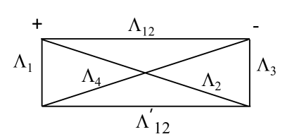
Figure 7.1: The Yutsis diagram reordering arguments of the $N=4$ isotropic function when $\Lambda_{1}$ shares a vertex with $\Lambda_{4}$; this stems from Eq. (256) with particular choices of the $Gi$. The three lines coming from the upper left and upper right vertices are given by the top rows of the first two 3-$j$ symbols in Eq. (256). The signs at these vertices are determined by the ordering of angular momenta in these first two 3-$j$ symbols. Our sign convention for the Yutsis diagrams is defined just below Eq. (6.3). The lines coming from, and the signs at, the lower left and right vertices are determined by the specific values of $G1,G2,G3,$ and $G4$. For instance, if $G1=1$ and $G2=4$ the lower left vertex should be marked with a $-$, reflecting that we must read the lines emanating from that vertex clockwise if we read them in the order dictated by the first 3-$j$ symbol in the last line of Eq. (256). If $G3=3$ and $G4=2$ the lower right vertex receives a $+$ mark, reflecting that we must read the lines emanating from that vertex counterclockwise if we read them in the order dictated by the second 3-$j$ symbol in the last line of Eq. (256). Comparing with Fig. C.1, the value of the diagram here, with $G1=1$, $G2=4$, $G3=3$, and $G4=2$, is given by a 6-$j$ symbol with no additional phase as shown in Table 7.2. Changing the order of $(G1,G2)$ introduces a phase $(-1)^{\Lambda_{G1}+\Lambda_{G2}+\Lambda^{\prime}_{12}}$ and similarly for changing the order of $(G3,G4)$. See Table 7.2.

Figure 7.2: The Yutsis diagram reordering arguments of the $N=4$ isotropic function when $\Lambda_{1}$ shares a vertex with $\Lambda_{3}$, that is, they occur in the same 3-$j$ symbol in the last line of Eq. (256). This diagram is the same as that in Fig. 7.1 save for switching $\Lambda_{3}$ with $\Lambda_{4}$. The orientations at the upper vertices are determined by the ordering of the angular momenta in the first two 3-$j$ symbols in Eq. (256). The signs at the lower vertices are determined by the $Gi$, appearing in the 3-$j$ symbols in the last line of Eq. (256). For instance, if $G1=1$ and $G2=3$, the lower lefthand vertex should be marked with a $-$. This sign is because reading in the order the momenta are listed in the relevant 3-$j$ symbol means going clockwise around the vertex. For the analogous reason, if $G3=4$ and $G4=2$, the lower righthand vertex receives a $+$ mark. Comparing this Figure with Fig. C.1, the value of the diagram is given by a 6-$j$ symbol, with the addition of the phase $(-1)^{\Lambda_{3}+\Lambda_{4}+\Lambda_{12}}$, required to bring the upper right vertex to its canonical value. See Table 7.3.

Prefactor: $\left\{\begin{array}[]{ccc}{\Lambda_{1}}&{\Lambda_{2}}&{\Lambda_{12}}\\ {\Lambda_{3}}&{\Lambda_{4}}&{\Lambda^{\prime}_{12}}\\ \end{array}\right\}\sqrt{(2\Lambda_{12}+1)(2\Lambda^{\prime}_{12}+1)}\prod_{i=1}^{4}\delta^{{\rm K}}_{\Lambda^{\prime}_{i}\Lambda_{Gi}}$

$F$	$G=F^{-1}$	phase
$(1234)\to(1342)$	$(1234)\to(1423)$	$(-1)^{\Lambda_{2}+\Lambda_{3}+\Lambda^{\prime}_{12}}$
$(1234)\to(1432)$	$(1234)\to(1432)$	$1$
$(1234)\to(2341)$	$(1234)\to(4123)$	$(-1)^{\Lambda_{1}+\Lambda_{2}+\Lambda_{3}+\Lambda_{4}}$
$(1234)\to(2431)$	$(1234)\to(4132)$	$(-1)^{\Lambda_{1}+\Lambda_{4}+\Lambda^{\prime}_{12}}$
$(1234)\to(3124)$	$(1234)\to(2314)$	$(-1)^{\Lambda_{2}+\Lambda_{3}+\Lambda^{\prime}_{12}}$
$(1234)\to(3214)$	$(1234)\to(3214)$	$1$
$(1234)\to(4123)$	$(1234)\to(2341)$	$(-1)^{\Lambda_{1}+\Lambda_{2}+\Lambda_{3}+\Lambda_{4}}$
$(1234)\to(4213)$	$(1234)\to(3241)$	$(-1)^{\Lambda_{1}+\Lambda_{4}+\Lambda^{\prime}_{12}}$

Table 7.2: Factor converting the $N=4$ isotropic functions to the standard ordering of angular arguments for eight permutations, all of which are proportional to one 6-$j$ symbol. The value of ${\cal B}^{F}_{\Lambda\Lambda^{\prime}}$ is given by the product of the prefactor and the phase of the corresponding permutation $F$. The diagram corresponding to this Table is given in Fig. 7.1.

Prefactor: $\left\{\begin{array}[]{ccc}{\Lambda_{1}}&{\Lambda_{2}}&{\Lambda_{12}}\\ {\Lambda_{4}}&{\Lambda_{3}}&{\Lambda^{\prime}_{12}}\\ \end{array}\right\}\sqrt{(2\Lambda_{12}+1)(2\Lambda^{\prime}_{12}+1)}\prod_{i=1}^{4}\delta^{{\rm K}}_{\Lambda^{\prime}_{i}\Lambda_{Gi}}$

$F$	$G=F^{-1}$	phase
$(1234)\to(1324)$	$(1234)\to(1324)$	$(-1)^{\Lambda_{2}+\Lambda_{3}+\Lambda_{12}+\Lambda^{\prime}_{12}}$
$(1234)\to(1423)$	$(1234)\to(1342)$	$(-1)^{\Lambda_{3}+\Lambda_{4}+\Lambda_{12}}$
$(1234)\to(2314)$	$(1234)\to(3124)$	$(-1)^{\Lambda_{1}+\Lambda_{2}+\Lambda_{12}}$
$(1234)\to(2413)$	$(1234)\to(3142)$	$(-1)^{\Lambda_{1}+\Lambda_{4}+\Lambda_{12}+\Lambda^{\prime}_{12}}$
$(1234)\to(3142)$	$(1234)\to(2413)$	$(-1)^{\Lambda_{2}+\Lambda_{3}+\Lambda_{12}+\Lambda^{\prime}_{12}}$
$(1234)\to(3241)$	$(1234)\to(4213)$	$(-1)^{\Lambda_{3}+\Lambda_{4}+\Lambda_{12}}$
$(1234)\to(4132)$	$(1234)\to(2431)$	$(-1)^{\Lambda_{1}+\Lambda_{2}+\Lambda_{12}}$
$(1234)\to(4231)$	$(1234)\to(4231)$	$(-1)^{\Lambda_{1}+\Lambda_{4}+\Lambda_{12}+\Lambda^{\prime}_{12}}$

Table 7.3: Factor converting the $N=4$ isotropic functions to the standard ordering of angular arguments for eight permutations, all of which are proportional to a second 6-$j$ symbol The value of ${\cal B}^{F}_{\Lambda\Lambda^{\prime}}$ is given by the product of the prefactor and the phase of the corresponding permutation $F$. The diagram corresponding to this Table is given in Fig. 7.2.

7.2 Reordering for $N=5$

By analogy with the $N=4$ case, we have for $N=5$ that

$${\cal B}^{F=G^{-1}}_{\Lambda,\Lambda^{\prime}}=\int d{\hat{\bf R}}\,{\cal P}_{\Lambda^{\prime}}({\hat{\bf r}}_{1},\ldots,{\hat{\bf r}}_{5}){\cal P}^{*}_{\Lambda}({\hat{\bf r}}_{F1},\ldots,{\hat{\bf r}}_{F5})$$

$$={\cal E}(\Lambda^{\prime})\sqrt{2\Lambda_{12}+1}\sqrt{2\Lambda^{\prime}_{12}+1}\sqrt{2\Lambda_{123}+1}\sqrt{2\Lambda^{\prime}_{123}+1}\prod_{i=1}^{5}\delta^{{\rm K}}_{\Lambda^{\prime}_{i}\Lambda_{Gi}}$$

$$\times\sum_{M_{i},M_{12},M^{\prime}_{12}\ldots}(-1)^{\Lambda_{12}-M_{12}+\Lambda_{123}-M_{123}+\Lambda^{\prime}_{12}-M^{\prime}_{12}+\Lambda^{\prime}_{123}-M^{\prime}_{123}}$$

$$\quad\times\left(\begin{array}[]{ccc}{\Lambda_{1}}\!&{\Lambda_{2}}\!&{\Lambda_{12}}\!\\ {M_{1}}\!&{M_{2}}\!&{-M_{12}}\!\\ \end{array}\right)\left(\begin{array}[]{ccc}{\Lambda_{12}}\!&{\Lambda_{3}}\!&{\Lambda_{123}}\!\\ {M_{12}}\!&{M_{3}}\!&{-M_{123}}\!\\ \end{array}\right)\left(\begin{array}[]{ccc}{\Lambda_{123}}\!&{\Lambda_{4}}\!&{\Lambda_{5}}\!\\ {M_{123}}\!&{M_{4}}\!&{M_{5}}\!\\ \end{array}\right)$$ (265)

$$\quad\times\left(\begin{array}[]{ccc}{\Lambda_{G1}}\!&{\Lambda_{G2}}\!&{\Lambda^{\prime}_{12}}\!\\ {-M_{G1}}\!&{-M_{G2}}\!&{-M^{\prime}_{12}}\!\\ \end{array}\right)\left(\begin{array}[]{ccc}{\Lambda^{\prime}_{12}}\!&{\Lambda_{G3}}\!&{\Lambda^{\prime}_{123}}\!\\ {M^{\prime}_{12}}\!&{-M_{G3}}\!&{-M_{123}}\!\\ \end{array}\right)$$ (270)

$$\qquad\qquad\qquad\times\left(\begin{array}[]{ccc}{\Lambda^{\prime}_{123}}\!&{\Lambda_{G4}}\!&{\Lambda_{G5}}\!\\ {M^{\prime}_{123}}\!&{-M_{G4}}\!&{-M_{G5}}\!\\ \end{array}\right).$$ (273)

Again, the factor ${\cal E}(\Lambda)$ and the power of $(-1)$ supply what is needed for a treatment with Yutsis diagrams. The situation is displayed in Fig. 7.3.

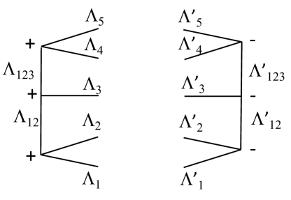
Figure 7.3: The Yutsis diagram reordering the arguments of an $N=5$ isotropic function. The permutation is not yet specified.

The values of ${\cal B}^{F}_{\Lambda\Lambda^{\prime}}$ fall into several distinct groups defined by the nature of the Yutsis diagram associated with the permutation $F$, leading to results that include a single 6-$j$ symbol, a product of two 6-$j$ symbols, a 9-$j$ symbol, or no such symbol.

Let us begin with a simple circumstance where $F$ is such that $G1=1,\;G2=2$. Then we can do the sum over $M_{1}$ and $M_{2}$ as before. This will leave us with

$${\cal B}^{F=G^{-1}}_{\Lambda,\Lambda^{\prime}} = \sqrt{2\Lambda_{123}+1}\sqrt{2\Lambda^{\prime}_{123}+1}\delta^{{\rm K}}_{\Lambda_{12}\Lambda^{\prime}_{12}}\sum_{M_{i},M_{12},M^{\prime}_{12}}(-1)^{\Lambda_{123}-M_{123}+\Lambda^{\prime}_{123}-M^{\prime}_{123}}$$ (283)

$$\quad\times\left(\begin{array}[]{ccc}{\Lambda_{12}}\!&{\Lambda_{3}}\!&{\Lambda_{123}}\!\\ {M_{12}}\!&{M_{3}}\!&{-m_{123}}\!\\ \end{array}\right)\left(\begin{array}[]{ccc}{\Lambda_{123}}\!&{\Lambda_{4}}\!&{\Lambda_{5}}\!\\ {M_{123}}\!&{M_{4}}\!&{M_{5}}\!\\ \end{array}\right)$$

$$\quad\times\left(\begin{array}[]{ccc}{\Lambda_{12}}\!&{\Lambda_{G3}}\!&{\Lambda^{\prime}_{123}}\!\\ {-m_{12}}\!&{-M_{G3}}\!&{-M_{123}}\!\\ \end{array}\right)\left(\begin{array}[]{ccc}{\Lambda^{\prime}_{123}}\!&{\Lambda_{G4}}\!&{\Lambda_{G5}}\!\\ {M^{\prime}_{123}}\!&{-M_{G4}}\!&{-M_{G5}}\!\\ \end{array}\right)\prod_{i=1}^{5}\delta^{{\rm K}}_{\Lambda^{\prime}_{i}\Lambda_{Gi}}.$$

In general, the condition $G1=1,\;G2=2$ yields a 6-$j$ symbol. For example, if $G(3)=4,G(4)=3$, and $G(5)=5$, so that $G$ maps $(12345)\to(12435)$, we will have the Yutsis diagram in Fig. 7.4.

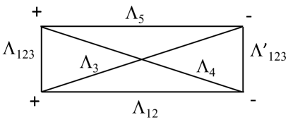
Figure 7.4: The Yutsis diagram reordering arguments of the $N=5$ isotropic function with the permutation $G$ that maps $(12345)\to(12435)$.

The 6-$j$ symbol is

$$\left\{\begin{array}[]{ccc}{\Lambda_{12}}&{\Lambda_{3}}&{\Lambda_{123}}\\ {\Lambda_{5}}&{\Lambda_{4}}&{\Lambda^{\prime}_{123}}\\ \end{array}\right\}$$ (284)

and there is a factor $(-1)^{\Lambda_{3}+\Lambda_{4}+\Lambda_{123}+\Lambda^{\prime}_{123}}$ arising from returning the vertex signs to canonical form.

7.2.1 Permutations requiring no 6-$j$ or 9-$j$ symbol

If, however, we choose a permutation like $G$: $(12345)\to(21345)$ we see that both the sum over $M_{1}$ and $M_{2}$ and the sum over $M_{4}$ and $M_{5}$ are trivial reductions. In particular, they are equivalent to the identity permutation up to an overall sign which is determined by the factors associated with the changes like $(12)\to(21)$. Clearly there are four such permutations in which each pair $(12)$ and $(45)$ transforms into itself. In addition, there are four more permutations like $G:(12345)\to(45312)$ in which $(1,2)$ and $(4,5)$ transform into each other. Thus there are eight permutations for which

$${\cal B}^{F}_{\Lambda,\Lambda^{\prime}}=\pm\delta^{{\rm K}}_{\Lambda_{12}\Lambda^{\prime}_{12}}\delta^{{\rm K}}_{\Lambda_{123}\Lambda^{\prime}_{123}}\prod\delta^{{\rm K}}_{\Lambda_{i},\Lambda_{Gi}}.$$ (285)

7.2.2 Permutations resulting in one 6-$j$ symbol

In contrast the number of permutations of the sort $G$: $(12345)\to(12435)$ in which $(12)$ transforms separately and $(345)$ transforms so that “3” is no longer in its original position is $2\times 4=8$. There are eight more of the form $G:(12345)\to(34512)$, where the $(12)$ pair are at the end. Similarly, there are 16 where we use $(45)$ in place of $(12)$. Altogether, there are 32 permutations giving rise to a 6-$j$ symbol.

7.2.3 Permutations yielding a 9-$j$ symbol

Now consider permutations that lead to no simple sums, i.e. neither pair $(12)$ or $(45)$ is left intact. In one class, $3$ is left in its original position, for example, $G$: $(12345)\to(14325)$. The Yutsis diagram is shown in Fig. 7.5.

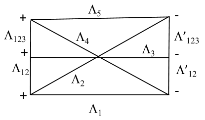
Figure 7.5: The Yutsis diagram reordering arguments of $N=5$ isotropic function with permutation $G:(12345)\to(14325)$. It is clear by comparison with Fig. C.2 that this is a 9-$j$ symbol.

Up to a sign and the factor

$$\sqrt{(2\Lambda_{12}+1)(2\Lambda^{\prime}_{12}+1)(2\Lambda_{123}+1)(2\Lambda^{\prime}_{123}+1)}$$ (286)

the result is

$$\left\{\begin{array}[]{ccc}{\Lambda_{12}}&{\Lambda_{1}}&{\Lambda_{2}}\\ {\Lambda_{123}}&{\Lambda_{4}}&{\Lambda_{5}}\\ {\Lambda_{3}}&{\Lambda^{\prime}_{12}}&{\Lambda^{\prime}_{123}}\end{array}\right\}.$$ (287)

There are 16 permutations in this class.

7.2.4 Permutations yielding two 6-$j$ symbols

Next consider permutations of the form $G$: $(12345)\to(31xxx)$ that have not been considered so far. The third element cannot be $2$ since this would leave the last two elements to be $(45)$ and these have already been counted. This leaves four possibilities. But in place of 1, we could use $2,4$ or $5$, each of which would itself provide four possibilities. Thus there are 16 new permutations beginning with $3$. But then we could equally well put the $3$ anywhere else but in its original position, so there are 64 permutations in this category.

An example is $G$: $(12345)\to(31425)$, whose diagram in shown in Fig. 7.6.

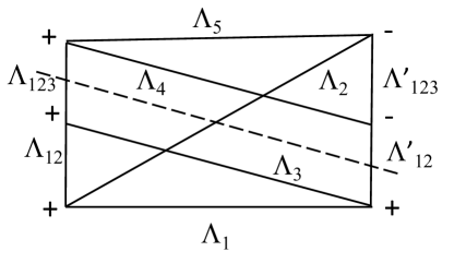
Figure 7.6: The Yutsis diagram reordering arguments of the $N=5$ isotropic functions. The permutation is $G:(12345)\to(31425)$. The dotted line shows how the figure can be split into two separate pieces while crossing only three lines. As a result, this diagram will represent the product of two 6-$j$ symbols.

Applying the factorization theorem described in Appendix D, which shows that a diagram that can be split into two separate pieces by a single cut crossing only three lines, we turn the diagram in Fig. 7.6 into the two diagrams shown in Fig. 7.7.

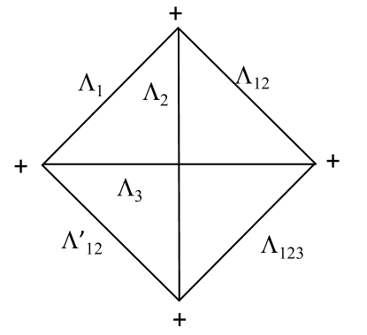
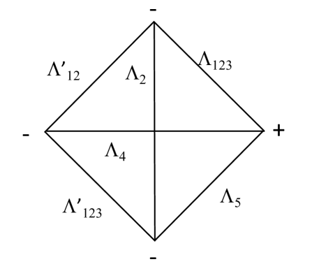
Figure 7.7: The two diagrams obtained by splitting Fig. 7.6. The signs do not have the canonical values, which would require alternating signs along the periphery.

The diagrams in Fig. 7.7 have the value

$$\left\{\begin{array}[]{ccc}{\Lambda_{1}}&{\Lambda_{2}}&{\Lambda_{12}}\\ {\Lambda_{123}}&{\Lambda_{3}}&{\Lambda^{\prime}_{12}}\\ \end{array}\right\}\left\{\begin{array}[]{ccc}{\Lambda^{\prime}_{12}}&{\Lambda_{2}}&{\Lambda_{123}}\\ {\Lambda_{5}}&{\Lambda_{4}}&{\Lambda^{\prime}_{123}}\\ \end{array}\right\}(-1)^{\Lambda_{1}+\Lambda_{3}+\Lambda_{4}+\Lambda^{\prime}_{123}}$$ (288)

where the phase arises from restoring the canonical signs at the vertices.

Altogether we have eight permutations leading to values of ${\cal B}^{F}_{\Lambda,\Lambda^{\prime}}$ that have no 6-$j$ or 9-$j$ symbols in their expression, 32 that are proportional to a single 6-$j$ symbol, 16 that lead to a 9-$j$ symbol and 64 of the sort we last considered. These account for all 120 permutations.

8 Summary

A complete basis set of isotropic functions of unit vectors ${\cal P}_{\Lambda}({\hat{\bf R}}={\hat{\bf r}}_{1},{\hat{\bf r}}_{2},\ldots,{\hat{\bf r}}_{N})$ is conveniently constructed from spherical harmonics and Clebsch-Gordan coefficients. The quantity $\Lambda$ is specified by $N$ primary angular momenta $\Lambda_{i}$ together with $N-3$ intermediate angular momenta $\Lambda_{12},\Lambda_{123},\ldots$ if $N>3$. The ${\cal P}_{\Lambda}$ are eigenfunctions of each ${\bf L}_{i}^{2}$ and of $({\bf L}_{1}+{\bf L}_{2})^{2},({\bf L}_{1}+{\bf L}_{2}+{\bf L}_{3})^{2},$ etc. Moreover, the ${\cal P}_{\Lambda}$ are orthonormal (§3). This basis set provides a convenient means of representing any isotropic function as

$$F_{\rm{iso}}({\bf R}) = \sum_{\Lambda}{\cal Z}_{\Lambda}(R){\cal P}_{\Lambda}({\hat{\bf R}}),$$

$${\cal Z}_{\Lambda}(R) = \int d{\hat{\bf R}}\,F_{\rm{iso}}({\bf R}){\cal P}^{*}_{\Lambda}({\hat{\bf R}})$$ (289)

with $R\equiv(r_{1},r_{2},\ldots,r_{N})=(|{\bf r}_{1}|,|{\bf r}_{2}|,\ldots,|{\bf r}_{N}|)$.

Because the ${\cal P}_{\Lambda}$ functions are complete it is always possible to express a product of two ${\cal P}_{\Lambda}$ functions as a sum over single ${\cal P}_{\Lambda}$ functions (§6):

$${\cal P}_{\Lambda}({\hat{\bf R}}){\cal P}_{\Lambda^{\prime}}({\hat{\bf R}})=\sum_{\Lambda^{\prime\prime}}{\cal E}(\Lambda^{\prime}){\cal G}^{\Lambda\Lambda^{\prime}\Lambda^{\prime\prime}}{\cal P}_{\Lambda^{\prime\prime}}({\hat{\bf R}})$$ (290)

where ${\cal E}(\Lambda^{\prime})=\sum_{i}\Lambda_{i}$ and ${\cal G}^{\Lambda\Lambda^{\prime}\Lambda^{\prime\prime}}$ can be computed in terms of 6-$j$ and 9-$j$ symbols. This is done conveniently with the diagrams developed by Yutsis et al. (1962). The quantity ${\cal G}^{\Lambda\Lambda^{\prime}\Lambda^{\prime\prime}}$ is a generalization of the Gaunt integral to which it corresponds for $N=2$.

Permuting the arguments ${\hat{\bf r}}_{1},\ldots,{\hat{\bf r}}_{N}\to{\hat{\bf r}}_{F1},\ldots,{\hat{\bf r}}_{FN}$ of a ${\cal P}_{\Lambda}$ function produces, in general, a new function that can be expressed in terms of the canonical basis (§7):

$${\cal P}_{\Lambda}({\hat{\bf r}}_{F1},\ldots,{\hat{\bf r}}_{FN})=\sum_{\Lambda^{\prime}}{\cal B}^{F}_{\Lambda,\Lambda^{\prime}}{\cal P}_{\Lambda^{\prime}}({\hat{\bf r}}_{1},\ldots,{\hat{\bf r}}_{N}).$$ (291)

The coefficients ${\cal B}^{F}_{\Lambda,\Lambda^{\prime}}$ (see Eq. 207) can be computed again in terms of 6-$j$ and 9-$j$ symbols using Yutsis diagrams.

These relations provide a powerful means of expressing multibody correlations and for calculating covariances between the correlations as explained in Slepian, Cahn & Eisenstein (in prep.).

Appendix A Cartesian representations of some rotationally invariant functions

It is instructive to examine explicit representations of some of the simplest ${\cal P}_{\Lambda}$ functions. These can be used to confirm some of the general relations obtained above. We indicate specific values of $\Lambda$ by the sequence $[\Lambda_{1},\Lambda_{2},(\Lambda_{12}),\Lambda_{3},(\Lambda_{123}),\ldots\Lambda_{N-1},\Lambda_{N}]$ since $\Lambda_{12\ldots N-1}=\Lambda_{N}$. Explicitly, we have

A.1 $N=2$

$${\cal P}_{00}({\hat{\bf r}}_{1},{\hat{\bf r}}_{2}) = \frac{1}{4\pi}$$

$${\cal P}_{11}({\hat{\bf r}}_{1},{\hat{\bf r}}_{2}) = -\frac{\sqrt{3}}{4\pi}({\hat{\bf r}}_{1}\cdot{\hat{\bf r}}_{2})$$

$${\cal P}_{22}({\hat{\bf r}}_{1},{\hat{\bf r}}_{2}) = \frac{3}{2}\sqrt{\frac{5}{(4\pi)^{2}}}\left[({\hat{\bf r}}_{1}\cdot{\hat{\bf r}}_{2})^{2}-\frac{1}{3}\right].$$ (A.1)

A.2 $N=3$

$${\cal P}_{110}({\hat{\bf r}}_{1},{\hat{\bf r}}_{2},{\hat{\bf r}}_{3}) = -\frac{1}{4\pi}\sqrt{\frac{3}{4\pi}}({\hat{\bf r}}_{1}\cdot{\hat{\bf r}}_{2})$$

$${\cal P}_{111}({\hat{\bf r}}_{1},{\hat{\bf r}}_{2},{\hat{\bf r}}_{3}) = -\frac{3i}{\sqrt{2}(4\pi)^{3/2}}{\hat{\bf r}}_{1}\cdot({\hat{\bf r}}_{2}\times{\hat{\bf r}}_{3})$$

$${\cal P}_{112}({\hat{\bf r}}_{1},{\hat{\bf r}}_{2},{\hat{\bf r}}_{3}) = \sqrt{\frac{27}{2(4\pi)^{3}}}\left[({\hat{\bf r}}_{1}\cdot{\hat{\bf r}}_{3})({\hat{\bf r}}_{2}\cdot{\hat{\bf r}}_{3})-\frac{1}{3}({\hat{\bf r}}_{1}\cdot{\hat{\bf r}}_{2})\right]$$

$${\cal P}_{222}({\hat{\bf r}}_{1},{\hat{\bf r}}_{2},{\hat{\bf r}}_{3}) = -\frac{45}{\sqrt{14(4\pi)^{3}}}\left[({\hat{\bf r}}_{1}\cdot{\hat{\bf r}}_{2})({\hat{\bf r}}_{1}\cdot{\hat{\bf r}}_{3})({\hat{\bf r}}_{2}\cdot{\hat{\bf r}}_{3})\right.$$ (A.2)

$$\left.-\frac{1}{3}({\hat{\bf r}}_{1}\cdot{\hat{\bf r}}_{2})^{2}-\frac{1}{3}({\hat{\bf r}}_{1}\cdot{\hat{\bf r}}_{3})^{2}-\frac{1}{3}({\hat{\bf r}}_{2}\cdot{\hat{\bf r}}_{3})^{2}+\frac{2}{9}\right].$$

A.3 $N=4$

$${\cal P}_{11(0)11}({\hat{\bf r}}_{1},{\hat{\bf r}}_{2},{\hat{\bf r}}_{3},{\hat{\bf r}}_{4}) = \frac{3}{(4\pi)^{2}}({\hat{\bf r}}_{1}\cdot{\hat{\bf r}}_{2})({\hat{\bf r}}_{3}\cdot{\hat{\bf r}}_{4})$$

$${\cal P}_{10(1)01}({\hat{\bf r}}_{1},{\hat{\bf r}}_{2},{\hat{\bf r}}_{3},{\hat{\bf r}}_{4}) = -\frac{\sqrt{3}}{(4\pi)^{2}}({\hat{\bf r}}_{1}\cdot{\hat{\bf r}}_{4})$$

$${\cal P}_{21(1)12}({\hat{\bf r}}_{1},{\hat{\bf r}}_{2},{\hat{\bf r}}_{3},{\hat{\bf r}}_{4}) = -\frac{9\sqrt{3}}{2(4\pi)^{2}}\left[({\hat{\bf r}}_{1}\cdot{\hat{\bf r}}_{2})({\hat{\bf r}}_{1}\cdot{\hat{\bf r}}_{4})({\hat{\bf r}}_{3}\cdot{\hat{\bf r}}_{4})-\frac{1}{3}({\hat{\bf r}}_{2}\cdot{\hat{\bf r}}_{4})({\hat{\bf r}}_{3}\cdot{\hat{\bf r}}_{4})\right.$$

$$\qquad\qquad\qquad\left.-\frac{1}{3}({\hat{\bf r}}_{1}\cdot{\hat{\bf r}}_{2})({\hat{\bf r}}_{1}\cdot{\hat{\bf r}}_{3})+\frac{1}{9}({\hat{\bf r}}_{2}\cdot{\hat{\bf r}}_{3})\right]$$

$${\cal P}_{21(2)12}({\hat{\bf r}}_{1},{\hat{\bf r}}_{2},{\hat{\bf r}}_{3},{\hat{\bf r}}_{4}) = \frac{3\sqrt{5}}{2(4\pi)^{2}}\left[2({\hat{\bf r}}_{1}\cdot{\hat{\bf r}}_{4})[({\hat{\bf r}}_{1}\cdot{\hat{\bf r}}_{4})({\hat{\bf r}}_{2}\cdot{\hat{\bf r}}_{3})-({\hat{\bf r}}_{1}\cdot{\hat{\bf r}}_{3})({\hat{\bf r}}_{2}\cdot{\hat{\bf r}}_{4})]\right.$$

$$\qquad\qquad\qquad-({\hat{\bf r}}_{1}\cdot{\hat{\bf r}}_{4})({\hat{\bf r}}_{1}\cdot{\hat{\bf r}}_{2})({\hat{\bf r}}_{3}\cdot{\hat{\bf r}}_{4})+({\hat{\bf r}}_{2}\cdot{\hat{\bf r}}_{4})({\hat{\bf r}}_{3}\cdot{\hat{\bf r}}_{4})$$

$$\qquad\qquad\qquad\qquad+\left.({\hat{\bf r}}_{1}\cdot{\hat{\bf r}}_{2})({\hat{\bf r}}_{1}\cdot{\hat{\bf r}}_{3})-({\hat{\bf r}}_{2}\cdot{\hat{\bf r}}_{3})\right]$$

$${\cal P}_{11(2)11}({\hat{\bf r}}_{1},{\hat{\bf r}}_{2},{\hat{\bf r}}_{3},{\hat{\bf r}}_{4}) = \frac{9}{2\sqrt{5}(4\pi)^{2}}\bigg{[}({\hat{\bf r}}_{1}\cdot{\hat{\bf r}}_{3})({\hat{\bf r}}_{2}\cdot{\hat{\bf r}}_{4})+({\hat{\bf r}}_{1}\cdot{\hat{\bf r}}_{4})({\hat{\bf r}}_{2}\cdot{\hat{\bf r}}_{3})$$

$$-\frac{2}{3}({\hat{\bf r}}_{1}\cdot{\hat{\bf r}}_{2})({\hat{\bf r}}_{3}\cdot{\hat{\bf r}}_{4})\bigg{]}$$

$${\cal P}_{11(1)11}({\hat{\bf r}}_{1},{\hat{\bf r}}_{2},{\hat{\bf r}}_{3},{\hat{\bf r}}_{4}) = \frac{3\sqrt{3}}{2(4\pi)^{2}}\left[({\hat{\bf r}}_{1}\cdot{\hat{\bf r}}_{3})({\hat{\bf r}}_{2}\cdot{\hat{\bf r}}_{4})-({\hat{\bf r}}_{1}\cdot{\hat{\bf r}}_{4})({\hat{\bf r}}_{2}\cdot{\hat{\bf r}}_{3})\right]$$

$${\cal P}_{21(1)10}({\hat{\bf r}}_{1},{\hat{\bf r}}_{2},{\hat{\bf r}}_{3},{\hat{\bf r}}_{4}) = \frac{3\sqrt{3}}{\sqrt{2}(4\pi)^{2}}\left[({\hat{\bf r}}_{1}\cdot{\hat{\bf r}}_{2})({\hat{\bf r}}_{1}\cdot{\hat{\bf r}}_{3})-\frac{1}{3}({\hat{\bf r}}_{2}\cdot{\hat{\bf r}}_{3})\right]$$

$${\cal P}_{21(3)12}({\hat{\bf r}}_{1},{\hat{\bf r}}_{2},{\hat{\bf r}}_{3},{\hat{\bf r}}_{4}) = -\frac{15}{2\sqrt{7}(4\pi)^{2}}\left[({\hat{\bf r}}_{1}\cdot{\hat{\bf r}}_{4})^{2}({\hat{\bf r}}_{2}\cdot{\hat{\bf r}}_{3})-\frac{4}{5}({\hat{\bf r}}_{1}\cdot{\hat{\bf r}}_{2})({\hat{\bf r}}_{1}\cdot{\hat{\bf r}}_{4})({\hat{\bf r}}_{3}\cdot{\hat{\bf r}}_{4})\right.$$

$$\qquad+2({\hat{\bf r}}_{1}\cdot{\hat{\bf r}}_{3})({\hat{\bf r}}_{1}\cdot{\hat{\bf r}}_{4})({\hat{\bf r}}_{2}\cdot{\hat{\bf r}}_{4})-\frac{2}{5}({\hat{\bf r}}_{1}\cdot{\hat{\bf r}}_{2})({\hat{\bf r}}_{1}\cdot{\hat{\bf r}}_{3})$$

$$\qquad\left.-\frac{2}{5}({\hat{\bf r}}_{2}\cdot{\hat{\bf r}}_{4})({\hat{\bf r}}_{3}\cdot{\hat{\bf r}}_{4})-\frac{1}{5}({\hat{\bf r}}_{2}\cdot{\hat{\bf r}}_{3})\right]$$

$${\cal P}_{21(2)11}({\hat{\bf r}}_{1},{\hat{\bf r}}_{2},{\hat{\bf r}}_{3},{\hat{\bf r}}_{4}) = i\frac{3\sqrt{3}}{2(4\pi)^{2}}\left[({\hat{\bf r}}_{1}\cdot{\hat{\bf r}}_{3})\ {\hat{\bf r}}_{4}\cdot({\hat{\bf r}}_{1}\times{\hat{\bf r}}_{2})+({\hat{\bf r}}_{1}\cdot{\hat{\bf r}}_{4})\ {\hat{\bf r}}_{3}\cdot({\hat{\bf r}}_{1}\times{\hat{\bf r}}_{2})\right]$$

$${\cal P}_{21(1)11}({\hat{\bf r}}_{1},{\hat{\bf r}}_{2},{\hat{\bf r}}_{3},{\hat{\bf r}}_{4}) = \frac{9i}{2(4\pi)^{2}}\left[({\hat{\bf r}}_{1}\cdot{\hat{\bf r}}_{2}){\hat{\bf r}}_{1}\cdot({\hat{\bf r}}_{3}\times{\hat{\bf r}}_{4})-\frac{1}{3}{\hat{\bf r}}_{2}\cdot({\hat{\bf r}}_{3}\times{\hat{\bf r}}_{4})\right].$$ (A.3)

Appendix B Properties of Wigner Angular Momentum Addition symbols

B.1 3-$j$ symbols

The 3-$j$ symbol or Wigner coefficient is defined in terms of the Clebsch-Gordan coefficient via

$$\left(\begin{array}[]{ccc}{j_{1}}\!&{j_{2}}\!&{j_{3}}\!\\ {m_{1}}\!&{m_{2}}\!&{m_{3}}\!\\ \end{array}\right)=\frac{(-1)^{j_{1}-j_{2}-m_{3}}}{\sqrt{2j_{3}+1}}\left<j_{1}m_{1}j_{2}m_{2}|j_{3}-m_{3}\right>.$$ (B.4)

The 3-$j$ symbols have the symmetries

$$\left(\begin{array}[]{ccc}{j_{1}}\!&{j_{2}}\!&{j_{3}}\!\\ {m_{1}}\!&{m_{2}}\!&{m_{3}}\!\\ \end{array}\right) = \left(\begin{array}[]{ccc}{j_{2}}\!&{j_{3}}\!&{j_{1}}\!\\ {m_{2}}\!&{m_{3}}\!&{m_{1}}\!\\ \end{array}\right)$$ (B.9)

$$= (-1)^{j_{1}+j_{2}+j_{3}}\left(\begin{array}[]{ccc}{j_{2}}\!&{j_{1}}\!&{j_{3}}\!\\ {m_{2}}\!&{m_{1}}\!&{m_{3}}\!\\ \end{array}\right)$$ (B.12)

$$= (-1)^{j_{1}+j_{2}+j_{3}}\left(\begin{array}[]{ccc}{j_{1}}\!&{j_{2}}\!&{j_{3}}\!\\ {-m_{1}}\!&{-m_{2}}\!&{-m_{3}}\!\\ \end{array}\right).$$ (B.15)

The orthogonality relation for 3-$j$ symbols is

$$\sum_{m_{2},m_{3}}\left(\begin{array}[]{ccc}{j_{1}}\!&{j_{2}}\!&{j_{3}}\!\\ {m_{1}}\!&{m_{2}}\!&{m_{3}}\!\\ \end{array}\right)\left(\begin{array}[]{ccc}{j_{4}}\!&{j_{2}}\!&{j_{3}}\!\\ {m_{4}}\!&{m_{2}}\!&{m_{3}}\!\\ \end{array}\right)=\frac{\delta^{{\rm K}}_{j_{1},j_{4}}\delta^{{\rm K}}_{m_{1},m_{4}}}{2j_{1}+1}.$$ (B.16)

Further summing the above result over $m_{1}$ yields

$$\sum_{m_{1},m_{2},m_{3}}\left(\begin{array}[]{ccc}{j_{1}}\!&{j_{2}}\!&{j_{3}}\!\\ {m_{1}}\!&{m_{2}}\!&{m_{3}}\!\\ \end{array}\right)\left(\begin{array}[]{ccc}{j_{1}}\!&{j_{2}}\!&{j_{3}}\!\\ {m_{1}}\!&{m_{2}}\!&{m_{3}}\!\\ \end{array}\right)=1.$$ (B.17)

B.2 6-$j$ symbols

The 6-$j$ symbol is

$$\left\{\begin{array}[]{ccc}{j_{1}}&{j_{2}}&{j_{3}}\\ {j_{4}}&{j_{5}}&{j_{6}}\\ \end{array}\right\}=\sum_{m_{1}\ldots m_{6}}(-1)^{\sum_{k}(j_{k}-m_{k})}\left(\begin{array}[]{ccc}{j_{1}}\!&{j_{2}}\!&{j_{3}}\!\\ {-m_{1}}\!&{-m_{2}}\!&{-m_{3}}\!\\ \end{array}\right)$$ (B.22)

$$\quad\times\left(\begin{array}[]{ccc}{j_{1}}\!&{j_{5}}\!&{j_{6}}\!\\ {m_{1}}\!&{-m_{5}}\!&{m_{6}}\!\\ \end{array}\right)\left(\begin{array}[]{ccc}{j_{4}}\!&{j_{2}}\!&{j_{6}}\!\\ {m_{4}}\!&{m_{2}}\!&{-m_{6}}\!\\ \end{array}\right)$$ (B.27)

$$\quad\times\left(\begin{array}[]{ccc}{j_{4}}\!&{j_{5}}\!&{j_{3}}\!\\ {-m_{4}}\!&{m_{5}}\!&{m_{3}}\!\\ \end{array}\right).$$ (B.30)

The 6-$j$ symbol is invariant under permutations of the columns and also under interchanging the top and bottom elements for any pair of columns.

If an element of a 6-$j$ symbol is zero there is a simplification. Using the rules for permuting rows and columns, a zero can always be brought to the lower right-hand position. The 6-$j$ symbol then becomes

$$\left\{\begin{array}[]{ccc}{j_{1}}&{j_{2}}&{j_{3}}\\ {j_{4}}&{j_{5}}&{0}\\ \end{array}\right\}=\frac{\delta^{{\rm K}}_{j_{2}j_{4}}\delta^{{\rm K}}_{j_{1}j_{5}}}{\sqrt{(2j_{1}+1)(2j_{2}+1)}}(-1)^{j_{1}+j_{2}+j_{3}}\delta^{{\rm K}}\left\{j_{1},j_{2},j_{3}\right\}.$$ (B.31)

where the final factor, $\delta^{{\rm K}}\left\{j_{1},j_{2},j_{3}\right\}$, is zero unless the three elements satisfy the triangular inequality.

It follows from the symmetries of the 6-$j$ symbol that

$$\left\{\begin{array}[]{ccc}{j_{1}}&{j_{2}}&{j_{3}}\\ {j_{4}}&{j_{5}}&{0}\\ \end{array}\right\}=\left\{\begin{array}[]{ccc}{j_{1}}&{j_{3}}&{j_{2}}\\ {j_{4}}&{0}&{j_{5}}\\ \end{array}\right\}=\left\{\begin{array}[]{ccc}{j_{3}}&{j_{1}}&{j_{2}}\\ {0}&{j_{4}}&{j_{5}}\\ \end{array}\right\}$$ (B.38)

$$\left\{\begin{array}[]{ccc}{j_{1}}&{j_{5}}&{0}\\ {j_{4}}&{j_{2}}&{j_{3}}\\ \end{array}\right\}=\left\{\begin{array}[]{ccc}{j_{1}}&{0}&{j_{5}}\\ {j_{4}}&{j_{3}}&{j_{5}}\\ \end{array}\right\}=\left\{\begin{array}[]{ccc}{0}&{j_{1}}&{j_{5}}\\ {j_{3}}&{j_{4}}&{j_{2}}\\ \end{array}\right\}.$$ (B.45)

Finally, we note that there is also a relationship between a 9-$j$ symbol where one element is zero and a 6-$j$ symbol (Eq. B.96).

B.3 9-$j$ symbols

The 9-$j$ symbol can be defined in a variety of ways. The expression in Edmonds (1996), 6.4.4, is the remarkably symmetric

$$\left\{\begin{array}[]{ccc}{j_{11}}&{j_{12}}&{j_{13}}\\ {j_{21}}&{j_{22}}&{j_{23}}\\ {j_{31}}&{j_{32}}&{j_{33}}\end{array}\right\}$$ (B.49)

$$\quad=\sum_{ms}\left(\begin{array}[]{ccc}{j_{11}}\!&{j_{12}}\!&{j_{13}}\!\\ {m_{11}}\!&{m_{12}}\!&{m_{13}}\!\\ \end{array}\right)\left(\begin{array}[]{ccc}{j_{21}}\!&{j_{22}}\!&{j_{23}}\!\\ {m_{21}}\!&{m_{22}}\!&{m_{23}}\!\\ \end{array}\right)\left(\begin{array}[]{ccc}{j_{31}}\!&{j_{32}}\!&{j_{33}}\!\\ {m_{31}}\!&{m_{32}}\!&{m_{33}}\!\\ \end{array}\right)$$ (B.56)

$$\quad\times\left(\begin{array}[]{ccc}{j_{11}}\!&{j_{21}}\!&{j_{31}}\!\\ {m_{11}}\!&{m_{21}}\!&{m_{31}}\!\\ \end{array}\right)\left(\begin{array}[]{ccc}{j_{12}}\!&{j_{22}}\!&{j_{32}}\!\\ {m_{12}}\!&{m_{22}}\!&{m_{32}}\!\\ \end{array}\right)\left(\begin{array}[]{ccc}{j_{13}}\!&{j_{23}}\!&{j_{33}}\!\\ {m_{13}}\!&{m_{23}}\!&{m_{33}}\!\\ \end{array}\right).$$ (B.63)

The 9-$j$ symbol is invariant under even permutations of its columns or rows. Under odd permutations it acquires a phase $(-1)^{J}$ where $J=\sum_{k}j_{k}$. It is also invariant under reflections about either diagonal.

Equivalently we have

$$\left\{\begin{array}[]{ccc}{j_{1}}&{j_{2}}&{j_{3}}\\ {k_{1}}&{k_{2}}&{k_{3}}\\ {\ell_{1}}&{\ell_{2}}&{\ell_{3}}\end{array}\right\} = \sum_{m_{i},n_{i},p_{i}}\left(\begin{array}[]{ccc}{j_{1}}\!&{j_{2}}\!&{j_{3}}\!\\ {m_{1}}\!&{m_{2}}\!&{m_{3}}\!\\ \end{array}\right)\left(\begin{array}[]{ccc}{k_{1}}\!&{k_{2}}\!&{k_{3}}\!\\ {n_{1}}\!&{n_{2}}\!&{n_{3}}\!\\ \end{array}\right)\left(\begin{array}[]{ccc}{\ell_{1}}\!&{\ell_{2}}\!&{\ell_{3}}\!\\ {p_{1}}\!&{p_{2}}\!&{p_{3}}\!\\ \end{array}\right)$$ (B.80)

$$\times\left(\begin{array}[]{ccc}{j_{1}}\!&{k_{1}}\!&{\ell_{1}}\!\\ {m_{1}}\!&{n_{1}}\!&{p_{1}}\!\\ \end{array}\right)\left(\begin{array}[]{ccc}{j_{2}}\!&{k_{2}}\!&{\ell_{2}}\!\\ {m_{2}}\!&{n_{2}}\!&{p_{2}}\!\\ \end{array}\right)\left(\begin{array}[]{ccc}{j_{3}}\!&{k_{3}}\!&{\ell_{3}}\!\\ {m_{3}}\!&{n_{3}}\!&{p_{3}}\!\\ \end{array}\right)$$

$$= \sum_{m_{i},n_{i},p_{i}}(-1)^{J}\left(\begin{array}[]{ccc}{j_{1}}\!&{j_{2}}\!&{j_{3}}\!\\ {m_{1}}\!&{m_{2}}\!&{m_{3}}\!\\ \end{array}\right)\left(\begin{array}[]{ccc}{k_{1}}\!&{k_{2}}\!&{k_{3}}\!\\ {n_{1}}\!&{n_{2}}\!&{n_{3}}\!\\ \end{array}\right)$$ (B.95)

$$\times\left(\begin{array}[]{ccc}{\ell_{1}}\!&{\ell_{2}}\!&{\ell_{3}}\!\\ {p_{1}}\!&{p_{2}}\!&{p_{3}}\!\\ \end{array}\right)\left(\begin{array}[]{ccc}{j_{1}}\!&{k_{1}}\!&{\ell_{1}}\!\\ {-m_{1}}\!&{-n_{1}}\!&{-p_{1}}\!\\ \end{array}\right)$$

$$\times\left(\begin{array}[]{ccc}{j_{2}}\!&{k_{2}}\!&{\ell_{2}}\!\\ {-m_{2}}\!&{-n_{2}}\!&{-p_{2}}\!\\ \end{array}\right)\left(\begin{array}[]{ccc}{j_{3}}\!&{k_{3}}\!&{\ell_{3}}\!\\ {-m_{3}}\!&{-n_{3}}\!&{-p_{3}}\!\\ \end{array}\right).$$

The 9-$j$ symbol with a lower right-hand zero becomes

$$\left\{\begin{array}[]{ccc}{j_{1}}&{j_{2}}&{j_{3}}\\ {j_{4}}&{j_{5}}&{j_{3}}\\ {j_{6}}&{j_{6}}&{0}\end{array}\right\}=\frac{(-1)^{j_{2}+j_{4}+j_{3}+j_{6}}}{\sqrt{(2j_{3}+1)(2j_{6}+1)}}\left\{\begin{array}[]{ccc}{j_{1}}&{j_{2}}&{j_{3}}\\ {j_{5}}&{j_{4}}&{j_{6}}\\ \end{array}\right\}.$$ (B.96)

It follows from the symmetries of the 9-$j$ symbol that

$$\left\{\begin{array}[]{ccc}{j_{1}}&{j_{2}}&{j_{3}}\\ {j_{4}}&{j_{5}}&{j_{3}}\\ {j_{6}}&{j_{6}}&{0}\end{array}\right\}=(-1)^{J}\left\{\begin{array}[]{ccc}{j_{1}}&{j_{3}}&{j_{2}}\\ {j_{4}}&{j_{3}}&{j_{5}}\\ {j_{6}}&{0}&{j_{6}}\end{array}\right\}=\left\{\begin{array}[]{ccc}{j_{3}}&{j_{1}}&{j_{2}}\\ {j_{3}}&{j_{4}}&{j_{5}}\\ {0}&{j_{6}}&{j_{6}}\end{array}\right\}$$ (B.106)

$$=(-1)^{J}\left\{\begin{array}[]{ccc}{j_{1}}&{j_{2}}&{j_{3}}\\ {j_{6}}&{j_{6}}&{0}\\ {j_{4}}&{j_{5}}&{j_{3}}\end{array}\right\}=\left\{\begin{array}[]{ccc}{j_{6}}&{j_{6}}&{0}\\ {j_{1}}&{j_{2}}&{j_{3}}\\ {j_{4}}&{j_{5}}&{j_{3}}\end{array}\right\}=(-1)^{J}\left\{\begin{array}[]{ccc}{j_{6}}&{0}&{j_{6}}\\ {j_{1}}&{j_{3}}&{j_{2}}\\ {j_{4}}&{j_{3}}&{j_{5}}\end{array}\right\}$$ (B.116)

$$=\left\{\begin{array}[]{ccc}{0}&{j_{6}}&{j_{6}}\\ {j_{3}}&{j_{1}}&{j_{2}}\\ {j_{3}}&{j_{4}}&{j_{5}}\end{array}\right\}=(-1)^{J}\left\{\begin{array}[]{ccc}{j_{3}}&{j_{1}}&{j_{2}}\\ {0}&{j_{6}}&{j_{6}}\\ {j_{3}}&{j_{4}}&{j_{5}}\end{array}\right\}=\left\{\begin{array}[]{ccc}{j_{1}}&{j_{3}}&{j_{2}}\\ {j_{6}}&{0}&{j_{6}}\\ {j_{4}}&{j_{3}}&{j_{5}}\end{array}\right\}.$$ (B.126)

Appendix C Yutsis diagrams

A Yutsis diagram (Yutsis et al., 1962) is defined by a product of Wigner coefficients, i.e. 3-$j$ symbols, in which every repeated $j$ occurs once with $m$ and once with $-m$. Every Wigner coefficient is assigned a point and two points are joined if they have a $j$ in common. At each point a $+$ or $-$ is assigned. If the $j$’s in the Wigner symbol, taken in left-to-right order, occur counter-clockwise in the diagram, one assigns a $+$ sign at the point. Otherwise one assigns a $-$ sign. We note that, in order for the initial expression to be described by a Yutsis diagram, the expression must have the phase

$$(-1)^{\sum_{i}(j_{i}-m_{i})}$$ (C.1)

for every $(j_{i},m_{i}),(j_{i},-m_{i})$ that appears in the collection, where $m_{i}$ is summed over.

Applying the rules for Yutsis diagrams to Eq. (B.30) we obtain Fig. C.1 representing

$$\left\{\begin{array}[]{ccc}{j_{1}}&{j_{2}}&{j_{3}}\\ {j_{4}}&{j_{5}}&{j_{6}}\\ \end{array}\right\}.$$ (C.2)

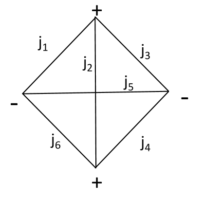
Figure C.1: The Yutsis diagram for a 6-$j$ symbol in canonical form.

Applying these rules to the 9-$j$ symbol in Eq. (B.95),

$$\left\{\begin{array}[]{ccc}{j_{1}}&{j_{2}}&{j_{3}}\\ {k_{1}}&{k_{2}}&{k_{3}}\\ {\ell_{1}}&{\ell_{2}}&{\ell_{3}}\end{array}\right\}$$ (C.3)

we obtain Fig. C.2.

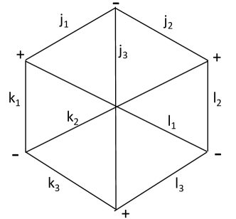
Figure C.2: Yutsis diagram showing the canonical 9-$j$ diagram; see Eq. (C.3). Note that changing sign at all vertices leaves the value unchanged because it introduces a factor $(-1)^{2\sum_{i}(j_{i}+k_{i}+\ell_{i})}=1$. Similarly, the mirror image diagram stands for the same 9-$j$ symbol.

Appendix D Yutsis Theorem on Factorization

Yutsis et al. (1962) prove a general theorem on the factorization of Yutsis diagrams that can be separated into two pieces by cutting through three or fewer lines. We need only a restricted version of the theorem, that which states that a product $R^{j_{1}j_{2}j_{3}}_{m_{1}m_{2}m_{3}}$ of 3-$j$ symbols summed over some indices but not summed over $m_{1},m_{2},m_{3}$ associated with $j_{1},j_{2},j_{3}$ can be written

$$R^{j_{1}j_{2}j_{3}}_{m_{1}m_{2}m_{3}}=\left(\begin{array}[]{ccc}{j_{1}}\!&{j_{2}}\!&{j_{3}}\!\\ {m_{1}}\!&{m_{2}}\!&{m_{3}}\!\\ \end{array}\right)R$$ (D.1)

where the value of $R$ is given by

$$R =\sum_{m_{i}}R^{j_{1}j_{2}j_{3}}_{m_{1}m_{2}m_{2}}\left(\begin{array}[]{ccc}{j_{1}}\!&{j_{2}}\!&{j_{3}}\!\\ {-m_{1}}\!&{-m_{2}}\!&{-m_{3}}\!\\ \end{array}\right)(-1)^{\sum_{i}(j_{i}-mi)}$$ (D.4)

$$=\sum_{m_{i}}R^{j_{1}j_{2}j_{3}}_{m_{1}m_{2}m_{2}}\left(\begin{array}[]{ccc}{j_{1}}\!&{j_{2}}\!&{j_{3}}\!\\ {m_{1}}\!&{m_{2}}\!&{m_{3}}\!\\ \end{array}\right)$$ (D.7)

where we recall that $\sum_{i}m_{i}=0$ and use Eqs. (B.15) and (B.17).

Figure D.1: A Yutsis diagram that can be separated into two separate diagrams by cutting just three lines can be written as the product of two simpler diagrams.

Now consider a diagram that can be separated by a single cut through three lines. Such a diagram can generically be represented by

$$\sum_{m_{i}} A^{j_{1}j_{2}j_{3}}_{m_{1}m_{2}m_{3}}B^{j_{1}j_{2}j_{3}}_{-m_{1}-m_{2}-m_{3}}(-1)^{\sum_{i}(j_{i}-m_{i})}$$ (D.14)

$$=\sum_{m_{i}}\left(\begin{array}[]{ccc}{j_{1}}\!&{j_{2}}\!&{j_{3}}\!\\ {m_{1}}\!&{m_{2}}\!&{m_{3}}\!\\ \end{array}\right)\left(\begin{array}[]{ccc}{j_{1}}\!&{j_{2}}\!&{j_{3}}\!\\ {-m_{1}}\!&{-m_{2}}\!&{-m_{3}}\!\\ \end{array}\right)(-1)^{\sum_{i}(j_{i}-m_{i})}AB$$

$$=AB.$$

The last line comes from the orthogonality relation for 3-$j$ symbols, Eq. (B.16). The signs to be attached to the diagrams for $A$ and $B$ will depend on the orientations of the lines for the $j_{i}$. In Fig. D.1 we see that the two separate diagrams will be identical to the two split pieces, but with a new vertex. In this example, the vertex attached to diagram A will have the opposite sign from the vertex attached to B. The phases introduced thereby will cancel.

References

Abramo &
Pereira (2010)
Abramo L. R., Pereira T. S., 2010, Advances in Astronomy, 2010, 1–25
Bartolo et al. (2004)
Bartolo N., Komatsu E., Matarrese S., Riotto A., 2004, Physics
Reports, 402, 103–266
Book
et al. (2012)
Book L. G., Kamionkowski M., Souradeep T., 2012, PRD, 85, 023010
Castorina &
White (2018)
Castorina E., White M., 2018, MNRAS, 476, 4,
4403–4417
Spergel &
Goldberg (1999)
Spergel D. N., Goldberg D. M., 1999, PRD, 59
Sugiyama
et al. (2018)
Sugiyama N. S., Saito S., Beutler F., Seo H.-J., 2018, MNRAS, 484, 364–384
Sugiyama
et al. (2020)
Sugiyama N. S., Saito S., Beutler F., Seo H.-J., 2020, Towards a
self-consistent analysis of the anisotropic galaxy two- and three-point
correlation functions on large scales: application to mock galaxy catalogues
(arXiv:2010.06179)
Tadros
et al. (1999)
Tadros H., et al., 1999, MNRAS,
305, 527
Verde
et al. (2000)
Verde L., Heavens A. F., Matarrese S., 2000, MNRAS, 318, 584–598