Improved Description of Atomic Environments using Low-cost Polynomial Functions with Compact Support

Abstract

The prediction of chemical properties using Machine Learning (ML) techniques calls for a set of appropriate descriptors that accurately describe atomic and, on a larger scale, molecular environments. A mapping of conformational information on a space spanned by atom-centred symmetry functions (SF) has become a standard technique for energy and force predictions using high-dimensional neural network potentials (HDNNP). An appropriate choice of SFs is particularly crucial for accurate force predictions. Established atom-centred SFs, however, are limited in their flexibility, since their functional form restricts the angular domain that can be sampled without introducing problematic derivative discontinuities. Here, we introduce a class of atom-centred symmetry functions based on polynomials with compact support called polynomial symmetry functions (PSF), which enable a free choice of both, the angular and the radial domain covered. We demonstrate that the accuracy of PSFs is either on par or considerably better than that of conventional, atom-centred symmetry functions. In particular, a generic set of PSFs with an intuitive choice of the angular domain inspired by organic chemistry considerably improves prediction accuracy for organic molecules in the gaseous and liquid phase, with reductions in force prediction errors over a test set approaching 50% for certain systems. Contrary to established atom-centred SFs, computation of PSF does not involve any exponentials, and their intrinsic compact support supersedes use of separate cutoff functions, facilitating the choice of their free parameters. Most importantly, the number of floating point operations required to compute polynomial SFs introduced here is considerably lower than that of other state-of-the-art SFs, enabling their efficient implementation without the need of highly optimised code structures or caching, with speedups with respect to other state-of-the-art SFs reaching a factor of 4.5 to 5. This low-effort performance benefit substantially simplifies their use in new programs and emerging platforms such as graphical processing units (GPU). Overall, polynomial SFs with compact support improve accuracy of both, energy and force predictions with HDNNPs while enabling significant speedups with respect to their well-established counterparts.

I Introduction

In the past decade, computational chemistry has seen a tremendous increase in use of machine learning (ML) techniques to overcome the length- and timescale problem burdening first principles methods[1, 2, 3, 4]. As such, ML techniques have seen particularly beneficial use in Molecular Dynamics (MD) simulations in the condensed phase. By providing highly elaborate fitting mechanisms, ML allows for accurate interpolation between training points on the potential energy surface (PES) generated from a computationally more expensive reference method. This enables, e.g. , MD simulations of water to be performed at the nano- rather than the picosecond scale with forces and energies of first principles accuracy[5, 6]. While still more expensive than classical force fields, ML techniques can incorporate information from the underlying PES well outside of local minima, making the simulation of chemical reactions possible. In contrast to reactive force-fields, no assumptions on the functional form of the interactions and therefore, the underlying PES, have to be made[7, 8]. Instead, the fit is carried out mostly in a black-box manner, with one of the most prominent adjustable input parameters being a set of functions that uniquely describe the environment of every atom in a manner that is invariant both to permutation, rotation and translation[4, 9, 10].

Machine learning techniques commonly used to interpolate between first principles data include kernel-based methods[11, 12, 13, 14] and neural network potentials (NNP)[15, 16]. A prominent framework of the latter is due to Behler and Parrinello[17, 18], who advocated the use of high-dimensional neural network potentials (HDNNP) in combination with atom-centred input functions. In the context of HDNNPs, these functions are commonly referred to as symmetry functions (SF)[19]. Ideally, these functions provide a unique description of the atomic environment of every structure in the training set. Several functional forms have been proposed[20, 21], which commonly include a radial and angular part multiplied by a cutoff function that ensures that the former are naught outside of predefined bounds. SFs are therefore commonly a product of up to three different types of functions, and parametrising them properly for a given chemical system can become non-trivial. An intuitive construction of SFs can be based on structural features of the system at hand. For instance, sufficient spatial resolution could be obtained by taking into account all relevant peaks in the radial distribution function of the system and by covering all chemically relevant angles spanned by an atom and two of its neighbours. The width and centre of a symmetry function should then reflect fluctuations of the quantity it describes in the training data. Such a strategy has successfully been used, e.g.  for the construction of a neural network of water and ice, including different ice phases[22, 23, 5].

However, whereas such a non-automated approach can yield symmetry function sets much smaller than those generated using automated procedures[21, 24], there are some pitfalls associated to an intuitive approach: While the position of the maxima of radial functions can generally be freely chosen within the cutoff radius, this is not necessarily the case for angular terms, which are commonly based on a cosine and which are therefore restricted to peak at either $0$ or $\pi$. Introducing a simple phase shift in the cosine has been shown to work well for energy evaluations[25], but it would be bound to fail for force predictions, since any shift in a cosine will inevitably introduce derivative discontinuities at $0$ and $\pi$: The evaluation of angles is restricted to a domain of $[0,\pi]$, imposing symmetries in the angular functions of the form $f(\vartheta)=f(-\vartheta)$ and $f(\pi+\vartheta)=f(\pi-\vartheta)$. Phase shifts break this symmetry and introduce non-zero derivatives at $f(0)$ and $f(\pi)$. Since derivatives of the angular functions are used to compute forces (vide infra), this results in non-unique descriptions at $\vartheta=0$ and $\vartheta=\pi$.

In order to account for equilibrium angles that are not centred on either peak and which only fluctuate over a few degress – such as a double bond – one therefore uses linear combinations of angular symmetry functions which are centred on either $0$ or $\pi$, increasing the overall number of SFs used. The presence of cutoff functions also obfuscates the choice of input SF parameters: If the SF are constructed from stuctural properties such as the radial distribution function of a liquid, the position of the radial peaks is not easily deduced from the input parameters, since the product of radial term and cutoff function may exhibit a shifted maximum and a more rapid decay with respect to the Gaussian function alone. In particular, if the Gaussian is not centred on the origin, this may lead to a symmetry function that is not symmetric with respect to its peak. Therefore, it is usually necessary to plot every single symmetry function in order to monitor the correspondence between the input parameters and the final system setup. Hence, parametrising symmetry functions based on structural properties can be a cumbersome procedure. While universal rules to generate input SFs have been proposed[21, 24], they often increase the number of SF needed with respect to an optimal, tailored set of parameters. This can hamper performance.

When using high-quality first principles methods to generate the training set, the first principle calculations usually represent the computational bottleneck. However, both the training of the neural network itself as well as its use in productive calculations carry a certain overhead that is typically larger than that of classical force fields. The computational cost of the training is in part associated to the number of symmetry functions used, as well as their computational complexity. While it is possible to store the values of all symmetry functions during training[26], making their calculation necessary only once at the very beginning of the training procedure, this is evidently impossible when the neural network potential is used to predict unknown structures e.g. during a MD run. Factors that contribute to the overhead of symmetry function evaluation are two-fold: The most popular choice for the radial term are Gaussian functions. However, exponentials are comparably expensive to compute. Furthermore, the calculation of a cutoff function (often cosines or hyperbolic tangents) introduces an additional overhead with respect to bare radial functions. To this end, optimised cutoff functions based on polynomials have already been proposed. Still, the disadvantages of the evaluation of exponentials for the radial terms, their possibly becoming asymmetric due to multiplication with a cutoff function and the impracticability of introducing phase shifts in the angular components remain. While strategies to reduce the large number of floating point operations during symmetry function evaluation have been developed, e.g. by grouping and caching[26, 27], this involves intermediate storage of quantities, loop breaks and many if-statements, rendering their implementation cumbersome, reducing code readability and making performance benefits both problem- and architecture dependent.

It would therefore be desirable to have a framework at hand where the number of floating point operations in SF evaluations is substantially reduced, where the SF remain symmetric with respect to their maxima, where the input parameters directly reflect the shape of the resulting function, and where the maximum of the angular component can be adjusted to reflect equilibrium angles. This would alleviate the need to plot every symmetry function during construction, making the resulting procedure more effecient and less error-prone, greatly simplifying the choice of parameters based on structural properties of the system at hand. Most importantly, a reduction of floating point operations supersedes the need of complex code optimisation and renders the efficient implementation of symmetry functions architecture-independent.

In the following, we will demonstrate that further simplifications to existing symmetry functions are possible by replacing the product-based ansatz of radial, angular and cutoff function by a product of polynomials with compact support, making the use of cutoff functions obsolete. Such polynomial symmetry functions have the advantage of allowing for angular terms to be centred anywhere within $\vartheta\in[0,\pi]$ without introducing derivative discontinuities at $\vartheta=0$ and $\vartheta=\pi$. The latter is of particular importance for force evaluations, as discontinutities in symmetry function derivatives will directly impact the forces computed. The evaluation of these polynomial symmetry functions does not involve exponentiation. Instead, the most demanding low-level operation becomes the calculation of an arccosine when computing angular terms. The use of one simple functional form for both angular and radial terms considerably reduces the number of floating point operations associated to the evaluation of a single SF. This does not only result in significant simplifications in the underlying code, but comes at the benefit of speedups of up to a factor of about 4.5 to 5, while their performance with respect to highly optimised cache and grouping based SF implementations still reaches a factor of almost 2 without the need of further algorithmic optimisations.

This text is organised as follows: First, we briefly introduce the concept of HDNNPs and describe the mathematical form of commonly used symmetry functions first proposed by Behler and Parrinello[17, 4]. We then introduce our new polynomial symmetry functions (PSF). We will go on to demonstrate that use of polynomial symmetry functions can improve accuracy of neural network potentials when compared to conventional symmetry functions. To this end, both dynamic and static properties will be compared for a water and copper sulfide model system. By training a HDNNP for the rotation of the amino group of the organic dye DMABN[28, 29], we will show that the angular flexibility of polynomial symmetry functions simplifies the choice of angular parameters compared to Behler-Parrinello type symmetry functions (BPSF). HDNNPs for liquid ethyl benzene and anisole that were trained using both PSF and PBSF will further support this perspective. Finally, we will show that use of PSF in conjunction with recently proposed weighted atom-centred symmetry functions (wACSF)[21] can further improve performance of HDNNPs for predicting enthalpies of formation of the QM9[30] database. We will conclude the discussion by comparing execution times for the evaluation of the NNPs between BPSFs and PSFs, showing that the execution time per symmetry function is substantially reduced for our polynomial ansatz.

II Symmetry Functions for High-Dimensional Neural Network Potentials

II.1 Neural Networks in a Nutshell

First applications of neural network potentials in computational chemistry date back as far as 1995[15]. A considerable advance in the prediction of molecular forces and energies was made in 2007, when Behler and Parrinello[17] proposed to use high-dimensional neural network potentials (HDNNP) in combination with a ficticious decomposition of the potential energy $V$ from $N$ individual atoms:

$$V=\sum_{i}^{N}V_{i}(\mathbf{G}_{i})$$ (1)

The atomic contribution $V_{i}$ depends on the chemical environment of atom $i$, which is described by a tuple of $N_{j}$ input values $\mathbf{G}_{i}=\{G_{1},\dots,G_{j}\}$. The forces on the $k$th atom follow from the gradient:

$$-\nabla_{k}V=-\sum_{i}^{N}\sum_{j}^{N_{j}}\frac{\partial V_{i}}{\partial G_{i,j}}\nabla_{k}G_{i,j}$$ (2)

The $\mathbf{G}_{i}$ are used as the input layer of a feed-forward neural network (Fig. 1) that yields the scalar $V_{i}$. The network itself is constituted by multiple layers of nodes, which are connected to each other by virtue of weights $a_{nm}$. Starting from a set of input values $(\mathbf{G}_{i})$, the data is propagated to node $n$ of hidden layer $k$ as follows:

$$y_{n}^{k}=f_{a}\left(b_{n}^{k}+\sum_{m}^{M_{l}}a_{nm}^{lk}y_{m}^{l}\right),$$ (3)

where $l=k-1$, $y_{n}^{k}$ represents the value of the node and $f_{a}$ is a non-linear activation function. $b_{n}^{k}$ denotes the bias associated to $y_{n}^{k}$ and $M_{l}$ is the number of neurons in layer $l$. One independent neural network per element is used. Together with the biases $b_{n}^{k}$, the weights $a_{nm}$ are the fitting parameters of the HDNNP.

The atomic environment descriptors $\mathbf{G}_{i}$ are commonly called symmetry functions (SF). In order to ensure permutational symmetry, the symmetry functions are identical for all atoms of the same element. However, in order to account for varying chemical environments (bond lengths, van-der-Waals radii, relevant bond angles), they can differ between different elements. An appropriate choice of symmetry functions is crucial in order to reliably discriminate between unique points on the PES.

Figure 1: Schematic representation of a Behler-Parrinello HDNNP for a given element $i$. Three symmetry functions $G_{i}$ are used as input, and the atomic contribution to the total potential energy $V_{i}$ is predicted. Labels correspond to Eq. 3.

Figure 2: Radial (left), angular (middle) and cutoff (right) functions proposed by Behler. Left: Due to the repulsive exchange wall, regions around $r=0$ are never sampled, and the radial function therefore need not be $0$ at $r=0$. Middle: A simple cutoff function with continuous derivatives at $0$ and $r_{c}$ is multiplied with the radial term to obtain a function with compact support. Note that this multiplication shifts the maxima of Gaussians that are not centred on $r_{0}=0$. Right: Minimum and maximum of the cosine are swapped for $\lambda=-1$. Specifying $\zeta>1$ contracts the function towards its maximum.

II.2 Behler-Parrinello Symmetry Functions

In the case of Behler-Parrinello HDNNPs, the input layer consists of scalars obtained from a predetermined set of atom-centred symmetry functions. The choice of symmetry functions should discriminate between all relevant structural features, such that every distinct point on the potential energy surface is described by a unique tuple of symmetry function values. In practice, this is achieved by combining a set of spherically symmetric and angle-dependent functions that have to be parametrised appropriately. Some examples are given in Fig. 2. For the radial part, Behler and Parrinello suggested:

$$f_{\text{B}}^{\text{rad}}(r,r_{s})=e^{-\eta(r-r_{s})^{2}},$$ (4)

where $r$ is an interatomic distance and $r_{s}$ its reference point. An angular dependency can by introduced by a function of the form:

$$f_{\text{B}}^{\text{ang}}(\vartheta,\lambda,\zeta)=\left(1+\lambda\cos(\vartheta)\right)^{\zeta},$$ (5)

where $\vartheta$ is the angle formed by any three atoms, bound by $[0,\pi]$. This function appropriately has $\partial f_{\text{B}}^{\text{ang}}/\partial\vartheta\lvert_{\vartheta=0}=\partial f_{\text{B}}^{\text{ang}}/\partial\vartheta\lvert_{\vartheta=\pi}=0$. For $\lambda=1$, maximum and minimum of the function lie at $0$ and $\pi$, respectively; for $\lambda=-1$, the inverse holds. Chosing $\zeta>1$ allows to contract the function, resulting in a more rapid decay. Values of $\zeta<1$ are not possible, since this would result in non-zero derivatives at the boundaries.

While the form of $f^{\text{ang}}_{\text{B}}(\vartheta,\lambda,\zeta)$ guarantees zero derivatives at the boundaries for appropriate choices of $\lambda$ and $\zeta$, the exponential in $f^{\text{rad}}_{\text{B}}(r,r_{c})$ is finite everywhere. Therefore, a cutoff function with cutoff radius $r_{c}$ is introduced, which ensures that the radial term and its derivatives are zero for all $r>r_{c}$. Common choices of cutoff function $f_{c}(r,r_{c})$ include

$$f_{c}(r,r_{c})=\begin{cases}\frac{1}{2}\left[\cos\left(\frac{\pi r}{r_{c}}\right)+1\right]\quad&\text{for}\quad r\leq r_{c}\\ 0\quad&\text{for}\quad r>r_{c}\end{cases}$$ (6)

or

$$f_{c}(r,r_{c})=\begin{cases}\tanh^{3}\left(1-\frac{r}{r_{c}}\right)\quad&\text{for}\quad r\leq r_{c}\\ 0\quad&\text{for}\quad r>r_{c}\end{cases}$$ (7)

Figure 3: Radial (upper rows) and angular (lower rows) symmetry functions of the Behler-Parrinello type. The reference atom $i$ is positioned at the origin. For radial functions, the plot shows the dependency of $f^{\text{rad}}_{B}$ on the position of neighbour $j$. For angular functions, it is assumed that one neighbouring atom $j$ has a fixed position at $x=0,y=1$, with the plot showing the dependency of $f^{\text{ang}}_{B}$ on the position of the second neighbour $k$.

With this choice of functions, the radial symmetry function $G_{i}$ centred on an atom $i$ is given by a sum over all its neighbours $j$ that are within a $r_{c}$ of $i$:

$$G_{i}^{\text{rad}}(r_{c},r_{s})=\sum_{j\neq i}f^{\text{rad}}_{\text{B}}(r_{ij},r_{s})f_{c}(r_{ij},r_{c}).$$ (8)

Note that such a product may have a width and a maximum different from $f^{\text{rad}}_{\text{B}}$ alone, see also Fig. 2. The angular symmetry function is constructed from a product of angular and radial terms, with the sum encompassing all neighbours $j$ and $k\neq j$. Depending on the radial term, two types of angular symmetry functions can be distinguished, namely narrow $n$,

$$G_{i}^{\text{ang.n}}(r_{c},r_{s},\lambda,\zeta)=2^{(1-\zeta)}\sum_{j\neq i,k>j}f^{\text{rad}}_{\text{B}}(r_{ij},r_{s})f^{\text{rad}}_{\text{B}}(r_{ik},r_{s})f^{\text{rad}}_{\text{B}}(r_{jk},r_{s})f^{\text{ang}}_{\text{B}}(\vartheta_{ijk},\lambda,\zeta)f_{c}(r_{ij},r_{c})f_{c}(r_{ik},r_{c})f_{c}(r_{jk},r_{c}),$$ (9)

which also constrains the interatomic distance between atoms $j$ and $k$, and the wide form $w$:

$$G_{i}^{\text{ang.w}}(r_{c},r_{s},\lambda,\zeta)=2^{(1-\zeta)}\sum_{j\neq i,k>j}f^{\text{rad}}_{\text{B}}(r_{ij},r_{s})f^{\text{rad}}_{\text{B}}(r_{ik},r_{s})f^{\text{ang}}_{\text{B}}(\vartheta_{ijk},\lambda,\zeta)f_{c}(r_{ij},r_{c})f_{c}(r_{ik},r_{c}),$$ (10)

the evaluation of which is more computationally expedient due to the lack of a radial term for $jk$. These symmetry functions have successfully been applied in a wide variety of contexts. Note that the distribution of symmetry function values at $\lambda=-1$ is not symmetric with respect to $\lambda=1$ due the presence of a radial function[21]. Fig. 3 displays the dependency of BPSFs on the position of atomic neighbour(s).

Recently, Singraber et al. have introduced a simple expression for $f_{c}$ based on polynomials[27]:

$$f_{c}^{\text{poly}}(r,r_{c})=\begin{cases}f^{\text{poly2}}\left(\frac{r}{r_{c}}\right)\quad&\text{for}\quad 0\leq r\leq r_{c}\\ 0\quad&\text{for}\quad r>r_{c}\end{cases}$$ (11)

with the polynomial:

$$f^{\text{poly2}}(x)=x^{3}(x(15-6x)-10)+1$$ (12)

with $f^{\text{poly2}}(0)=1$ and $f^{\text{poly2}}(1)=0$. At $x=0$ and $x=1$, Eq. 12 has continuous derivatives up to second order, which ensures a continuous, smooth transition to outside of the compact set. Similar polynomials with continuous derivatives up to even higher order can be easily constructed[27], but their use does not result in any practical benefit[18]. The main advantage of polynomial cutoff functions as introduced in Ref. 27 lies in their expedient evaluation compared to expressions based on hyperbolic tangent or cosine, reducing the overhead due to the cutoff function. However, the computation of costly exponentials is still needed for all radial components. Hence, a grouping strategy was proposed in Ref. 27 which avoids multiple evaluations of the same exponential term, resulting in considerable speedups.

II.3 Polynomial Symmetry Functions with Compact Support

Figure 4: Radial PSF (left), radial PAS (middle) and angular (right) SFs with compact support proposed here. Left: Radial function with point-symmetry around $0.5r_{\text{max}}$. Note that no cutoff function is needed, which enables a precise choice of maxima and shifts. Middle: Asymmetryic radial function with longer tail, with a shape comparable to the product of a Gaussian and a cutoff function in Fig. 2. Right: Angular polynomial SF. Note that the angular domain can be freely chosen and does not need to have maxima at $0$ or $\pi$.

On one hand, the summation over the arguments of $G^{\text{ang}}$ still involves a substantial number of exponential functions that have to be explicitly evaluated even when a grouping strategy is used. On the other hand, the present choice of $f^{\text{ang}}$ implies that, in order to specifically sample angles which are not centred close to either $0$ or $\pi$, a combination of several values of $\lambda$ and $\zeta$ is necessary, since introducing an angular shift $\vartheta_{0}$ would inevitably violate the boundary condition $\partial f^{\text{ang}}/\partial\vartheta=0$ at the bounds of the angular domain. In the following, we will attempt to overcome this issue by constructing a simple set of symmetry functions based on polynomials with compact support which can be used to indiscriminately describe both anglular and radial dependencies.

In order to do so, we generalise Eq. 11 to a generic form, expressed in terms of the boundaries $x_{\text{min}},x_{\text{max}}$ of the underlying domain. In particular, for our polynomial symmetry functions $f_{\text{PSF}}$, we also allow for arguments $x<0$:

$$f_{\text{PSF}}(x,x_{0},\Delta x)=\begin{cases}f^{\text{poly2}}\left(\frac{x-x_{0}}{\Delta x}\right)\quad&\text{for}\quad x_{0}\leq x\leq x_{0}+\Delta x\\ f^{\text{poly2}}\left(\frac{x_{0}-x}{\Delta x}\right)\quad&\text{for}\quad x_{0}-\Delta x\leq x<x_{0}\\ 0\quad&\text{elsewhere}\end{cases}$$ (13)

where $x_{0}=\frac{1}{2}(x_{\text{max}}+x_{\text{min}})$ and $\Delta x=\frac{1}{2}(x_{\text{max}}-x_{\text{min}})$. The resulting function is symmetric with respect to $x_{0}$ and has continuous derivatives – up to an order determined by the construction of $f^{\text{poly2}}$ – on all $\mathbb{R}^{3}$. It is possible to further influence the decay of the radial function by appropriately modifying its argument such that the symmetry function decays more rapidly around its maximum while also approaching $0$ more slowly, thus breaking the point symmetry around $f_{\text{PSF}}(0.5)$. We therefore define the asymmetric polynomial symmetry function (PAS) as:

$$f_{\text{PAS}}(x,x_{0},\Delta x)=\begin{cases}f^{\text{poly2}}\left(\frac{2(x-x_{0})}{\Delta x}-\left(\frac{x-x_{0}}{\Delta x}\right)^{2}\right)\quad&\text{for}\quad x_{0}\leq x\leq x_{0}+\Delta x\\ f^{\text{poly2}}\left(\frac{2(x_{0}-x)}{\Delta x}-\left(\frac{x_{0}-x}{\Delta x}\right)^{2}\right)\quad&\text{for}\quad x_{0}-\Delta x\leq x<x_{0}\\ 0\quad&\text{elsewhere}\end{cases}$$ (14)

which offers the same benefits as $f_{\text{PSF}}$ for $x\in[0,1]$. By construction, $f_{\text{PAS}}$ resembles the shape of the product of a local, narrow Gaussian function with a cutoff function and can therefore be used to adapt existing BPSF-setups to polynomial form. The functional forms of $f_{\text{PAS}}$ and $f_{\text{PSF}}$ are depicted in Fig. 4.

Figure 5: Radial (upper rows) and angular (lower rows) symmetry functions of the PAS type. The reference atom $i$ is positioned at the origin. For radial functions, the plot shows the dependency of $f^{\text{rad}}_{B}$ on the position of neighbour $j$. For angular functions, it is assumed that one neighbouring atom $j$ has a fixed position at $x=0,y=1$, with the plot showing the dependency of $f^{\text{ang}}_{B}$ on the position of the second neighbour $k$. Note that with PSF and PAS it becomes possible to cover specific angular ranges associated, e.g. to double bonds ($60^{\circ}$ angle, lower middle) or tetrahedra ($109.1^{\circ}$, lower right).

The corresponding radial symmetry functions can now be constructed as:

$$G_{i}^{\text{rad/P}}=\sum_{j\neq i}f_{\text{P}}(r_{ij},r_{s},\Delta r).$$ (15)

with $f_{\text{P}}$ either $f_{\text{PSF}}$ or $f_{\text{PAS}}$. Their narrow angular counterparts read:

$$G_{i}^{\text{ang.n/P}}=\sum_{j\neq i,k>j}f_{\text{P}}(r_{ij},r_{s},\Delta r)f_{\text{P}}(r_{ik},r_{s},\Delta r)f_{\text{P}}(r_{jk},r_{s},\Delta r)f_{\text{PSF}}(\vartheta_{ijk},\vartheta_{0},\Delta\vartheta)$$ (16)

while the wide angular functions become:

$$G_{i}^{\text{ang.w/P}}=\sum_{j\neq i,k>j}f_{\text{P}}(r_{ij},r_{s},\Delta r)f_{\text{P}}(r_{ik},r_{s},\Delta r)f_{\text{PSF}}(\vartheta_{ijk},\vartheta_{0},\Delta\vartheta)$$ (17)

where the radial component $f_{\text{P}}$ can again be described by both $f_{\text{PAF}}$ or $f_{\text{PSF}}$. Both types of angular symmetry function can be centred anywhere within $[0,\pi]$, provided that $\partial f_{\text{PSF}}/\partial\delta\lvert_{\vartheta=0}=0$ and $\partial f_{\text{PSF}}/\partial\delta\lvert_{\vartheta=\pi}=0$. This enables chemically intuitive choices of angular maxima, i.e. $60^{\circ}$ for a double bond or $109,4^{\circ}$ for a carbon-carbon single bond. Fig. 5 shows the dependency of PAS-type symmetry functions on the position of atomic neighbour(s).

Eqs 13 to 14 do not involve any exponentials, and the most expensive arithmetic operation, an inverse cosine, has a modest computational footprint.

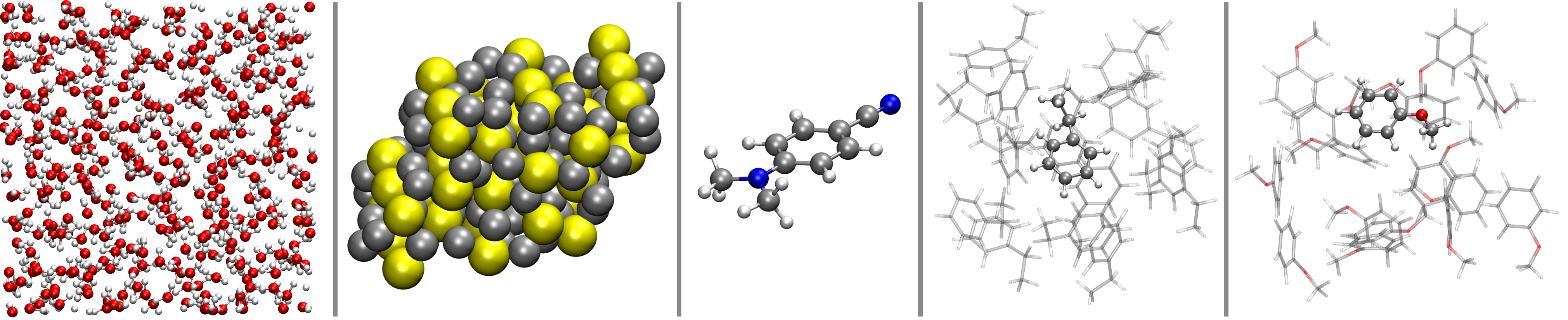
Figure 6: Systems studied here. From left to right: Water, Cu₂S, DMABN, liquid ethyl benzene and anisole.

III Computational Methods

III.1 Training of the HDNNP

All HDNNPs were trained using the n2p2 package[27, 26, 31]. HDNNPs for the prediction of enthalpies of formation in the QM9[30] database were obtained using the protocol of Ref. 21 with five-fold cross validation, but without dataset normalisation. For the remaining setups, 10 training runs per system are carried out with an independent seed for the random number generator each. If the value $G^{i}$ of a given symmetry function never exceeds $10^{-3}$ over the whole test set, the function is discarded before training. The choice of $G^{i}$ is detailed in the Supporting Information. Results discussed in this text refer to the best set of weights out of 10 independent runs (5 for the QM9 set), which are defined as the weights that yield the lowest force root mean-square deviation (RMSD) with respect to a test set constituted by 10% of training-set structures that were randomly removed before training. If several sets of weights yield force RMSDs that are identical to a few %, the set that displays the lowest relative error in energy predictions is used.

III.2 Training Sets

The systems investigated here are depicted in Fig. 6. The training sets for water and copper sulphide correspond to those published in Refs 5 and 26, respectively. Forces and energies for an isolated DMABN molecule, liquid ethyl benzene and anisole (16 molecules in a periodic box) were obtained from high-temperature Car-Parrinello Molecular Dynamics runs performed with the CPMD code[32] using the SCAN exchange-correlation functional[33]. The amino group of DMABN was rotated using a slowly growing harmonic restraint, giving rise to a set of non-equilibrium conformers. Details on the computational setup can be found in the Supporting Information.

 

Figure 7: Force predictions on water set of Ref. 26. Ref denotes references forces and nnp the prediction by the HDNNP. Left: Logarithmic learning curve showing the decrease of the RMSD between predicted and reference forces as a function of training steps (epochs). There are no appreciable differences between BPSF, PSF and PAS. A thin line denotes the target RMSD of 50 meV / Å. Right: Distribution $P(\Delta F)$ of relative force errors, $(\Delta F=F_{\text{nnp}}-F_{\text{ref}})/F_{\text{ref}}$ for BPSF, PSF and PAS.

III.3 Test Sets

Test sets consists of 10% randomly chosen configurations that are removed from the training set before training and which are then used to validate the predictive power of the neural network potential.

III.4 Molecular Dynamics using Neural Network Potentials

All MD simulations using HDNNPs were carried out using the n2p2-interface[27, 31] to the LAMMPS code[34, 35]. System setups are detailed in the Supporting Information.

IV Results and Discussion

IV.1 Water

We first assess the accuracy that can be attained with polynomial SFs by comparing the efficiency and accuracy of both training and productive simulations using identically set up HDNNPs. Two setups of polynomial SFs will be used: One, PSF, consisting entirely of symmetric functions of the form 13, and one mixed setup, PAS, including both symmetric and asymmetric radial components. We will compare against a reference setup using BPSFs, which has successfully been used in Ref. 26 to describe the PES of water and several ice phases. PSF and PAS were constructed by plotting the BPSFs and using their peaks and the full width at half maximum as rough indicators for the polynomial input. For sake of simplicity, the only symmetric radial terms (PSF-type) in the PAS set were those with maximum width; all others were chosen to be of the antisymmetric type.

Figure 8: Properties of water obtained during a molecular dynamics run with HDNNPs trained using BPSF, PSF and PAS. Left: Oxygen-oxygen radial distribution function $g(r)$ averaged over a 2 ns NVT trajectory. $g(r)$ obtained using different symmetry functions practically show no difference. Right: Mean-squared displacements and errors obtained over 2 ns of MD in the NVE ensemble. Error margins for all lines overlap, suggesting equivalency between all symmetry functions investigated here.

First, we compare the learning curves of both methods to assess the efficiency of the training procedure. Here, we define the learning curve as the RMSD between trained energy and forces and their reference as a function of the number of training steps (epochs). Curves for Behler-Parrinello type and polynomial SF setups are plotted in Fig. 7 and are virtually indistinguishable, suggesting that both types of symmetry functions can be trained with equal efficiency. RMSDs at the last training step are comparable between different methods, with the largest remaining force deviation being observed for the PSF setup. Conversely, the lowest force RMSD is observed for the PAS setup. BPSFs yield a training error intermediate between PAS and PSF data.

Figure 9: Predicted (nnp) vs. reference (ref) forces as obtained using BPSF, PSF and PAS. A deviation from the diagonal indicates an error in the force prediction. PAS and PSF further improve the description of the forces largest in magnitude. Absolute deviations from the diagonal are plotted in the top panel.

The same conclusion holds when analysing the distribution of both force and energy errors within the test set: Force RMSDs are 43.7 meV/Å for BPSFs, 48.5 meV/Å for PSF and 43.2 meV/Å for PAS, respectively. Energy RMSDs range from 1.17 meV fo BPSFs to 0.95 meV for PAS. In practical applications, these values could be considered identical. In Fig. 7, we histogram both the relative force error for HDNNPs trained with Behler-Parrinello type and polynomial SFs. The resulting distributions for the test set compare well between PSF, PAS and BPSF: All relative errors show a rapid decay, indicating an excellent quality of the fit. PAS and BPSF show very similar relative error distributions, whereas the distribution of PSF skews very lightly towards the right; however, we will show that this is of no practical relevance. Fig. 9 shows predicted forces against their reference values; ideally, all values should lie on a diagonal. Use of PAS and PSF improves the accuracy of the most extreme force values at either end of the graph, which lie closer to the diagonal than for BPSF. This indicates that, although force RMSDs differ only little between the different SF setups, qualitative improvements to conventional BPSFs are possible by use of a PSF or PAS set.

Fig. 8 provides a practical comparison of the predictive power of the different networks. Both the radial distribution function (left panel) as well as the mean square displacement as a function of time, from which the diffusion coefficient can be derived, (right panel) are practically indistinguishable between BPSF, PAS and PSF. These results further support that polynomial SFs are a viable alternative to the commonly used Behler-Parrinello type functions. The excellent agreement between radial distribution functions and mean-squared displacements obtained from Molecular Dynamics suggest that the small differences in force RMSD over the test set do not entail significant changes in the quality of the predictions made by the HDNNP. Notably, the mean-squared displacements (MSD) for PSF and BPSF are virtually identical.

Figure 10: Force predictions on the Cu₂S test set corresponding to 10% of the structures of the training set of Ref. 26. Ref denotes references forces and nnp the prediction by the HDNNP. Left: Predicted (nnp) vs. reference (ref) forces as obtained using BPSF, PSF and PAS. Shown are the forces largest in magnitude. A deviation from the diagonal indicates an error in the force prediction. PAS and PSF are better able to train the largest forces in the test set, which is reflected in a smaller deviation from the diagonal. Right: Distribution $P(\Delta F)$ of relative force errors, $(\Delta F=F_{\text{nnp}}-F_{\text{ref}})/F_{\text{ref}}$ for BPSF, PSF and PAS.

Figure 11: Force prediction quality for an isolated DMABN molecule, including a rotation of its amino group along a non-equilibrium path. Left: Predicted (nnp) vs. reference (ref) forces as obtained using BPSF, PSF and PAS. A deviation from the diagonal indicates an error in the force prediction. PAS forces remain closer to the diagonal than either BPSF and PSF. Right: Distribution $P(\Delta F)$ of relative force errors, $(\Delta F=F_{\text{nnp}}-F_{\text{ref}})/F_{\text{ref}}$ for BPSF, PSF and PAS. Whereas the distribution for BPSF and PAS are similar, PSF again skew slightly towards the right.

IV.2 Copper sulfide

All symmetry function setups used for water were based on the optimised, hand-selected set of Ref. 5. Such a selection by hand may not always be possible. In the following, we shall further validate the accuracy of PSF and PAS by comparing their performance to the accuracy of a semi-automatically generated set of BPSFs for copper sulfide. It has been show in Ref. 26 that a HDNNP with BPSFs can be successfully used to observe structural phase transitions in this compound.

Fig. 10 compares absolute and relative force errors obtained using BPSFs of Ref. 26 as well as our PSF and PAS. Force RMSDs are 51.9 meV/Å for BPSF, 56.7 meV/Å for PSF and 52.3 meV/Å for PAS, which corresponds roughly to a 10% difference between PSF and BPSF. Again, the performance of BPSF and PAS is on par, whereas use of PSF leads to slightly larger errors, which is also reflected in the relative error distribution skewing lightly to the right. Overall, however, this effect is expected to remain negligible in practical applications. Deviations from the diagonal in the graph comparing prediction and reference forces (Fig. 10, right panel) do not exhibit visible differences, further indicating that the general performance of all symmetry function types investigated here remains comparable and that the differences in force RMSDs observed here are not expected to influence the quality of the predictions in a significant manner. Energy RMSDs remain similar for all methods, spanning a range from 0.99 meV for PAS to 1.06 meV for BPSF.

IV.3 Organic molecules: Gas phase and liquids

In the following, we shall compare the performance of BPSFs generated according to Ref. 24 with our polynomial symmetry functions using an isolated (gas-phase) DMABN molecule and liquid ethyl benzene. We note that optimal symmetry function setups could possibly be found for all SF types investigated here; however, since this is a time-intensive procedure, the main purpose of this comparison is to compare the out-of-the-box performance of some generic sets of SFs.

Figure 12: Force prediction for ethyl benzene in its liquid state. Left: Predicted (nnp) vs. reference (ref) forces as obtained using BPSF, PSF and PAS. A deviation from the diagonal indicates an error in the force prediction. PAS forces remain closer to the diagonal than either BPSF and PSF. Right: Distribution $P(\Delta F)$ of relative force errors, $(\Delta F=F_{\text{nnp}}-F_{\text{ref}})/F_{\text{ref}}$ for BPSF, PSF and PAS. Whereas the distribution for PSF and PAS are similar, BPSFs skew considerably to the right, indicating a substantial difference in accuracy.

Figure 13: Force prediction for liquid anisole. Left: Predicted (nnp) vs. reference (ref) forces as obtained using BPSF, PSF and PAS. A deviation from the diagonal indicates an error in the force prediction. PAS forces remain closer to the diagonal than either BPSF and PSF. Right: Distribution $P(\Delta F)$ of relative force errors, $(\Delta F=F_{\text{nnp}}-F_{\text{ref}})/F_{\text{ref}}$ for BPSF, PSF and PAS. Whereas the distribution for BPSF and PAS are similar, PSF skew slightly towards the right. However, this difference is much less pronounced than the one observed for BPSF in Fig. 12.

To this end, we introduce a simple generation scheme for radial symmetry function parameters given a minimal and maximum width, $\Delta_{\text{min}}$ and $\Delta_{\text{max}}$, and a maximum cutoff radius $r_{c}$. For $N_{0}$ symmetry functions which are symmetric w.r.t to the origin, we choose the width $\Delta^{i}_{0}$ parameters of the $i$-th out of $N_{0}$ PSF or PAS as:

$$\Delta^{0}_{0} =r_{c}$$ (18)

$$\Delta^{i}_{0} =\Delta_{\text{max}}-\frac{(i-1)(\Delta_{\text{max}}-\Delta_{\text{min}})}{N_{0}-2}\quad;\quad i\geq 1$$ (19)

For a given number $N_{s}$ of symmetry functions which are centred at $r_{s}^{i}\neq 0$, we obtain shifts and widths $\Delta^{i}_{s}$ as:

$$\Delta^{i}_{s} =\frac{2r_{c}}{N_{s}+1}$$ (20)

$$r_{s}^{i} =\frac{(i-1)\Delta^{i}_{s}}{2}$$ (21)

This partitioning is reminiscent to the one introduced by Gastegger et al in Ref. 21. Angles were chosen to reflect common structural features encountered in organic chemistry: Linearity for triple bonds, $60^{\circ}$ and $109.1^{\circ}$ angles to describe double- and single carbon-carbon bonds, respectively. This resulted in the following angular functions: $\vartheta_{0}^{1}=0^{\circ}$, $\vartheta_{1}^{1}=90^{\circ}$ and $\vartheta_{3}^{1}=180^{\circ}$ with $\Delta\vartheta^{1,2,3}=90^{\circ}$; $\vartheta_{0}^{4}=60^{\circ}$, $\vartheta_{0}^{5}=120^{\circ}$ and $\vartheta_{0}^{6}=109.1^{\circ}$ with $\Delta\vartheta^{4,5,6}=60^{\circ}$ each. For sake of comparison, the cutoff function distance for BPSFs and the maximum extent of PAS and PSF were set to 15 a.u.

Structures in the DMABN-set cover regions of the PES thermally accessible at 1320K, including a forced rotation around the amino group along a non-equilibrium path. This results in many forces with large magnitude which are well outside of the equilibrium regime in which simple harmonic potentials can also yield good approximations. The DMABN set therefore serves as an assessment for the transferability of our polynomial SFs to structures which are considerably off-equilibrium.

Force RMSDs on the test set amount to 63.2 meV/Å for BPSF, 56.6 meV/Å for PSF and 54.0 meV/Å for PAS. This difference is directly reflected in the right panel of Fig. 11, where the force histograms show an increasing spread towards larger values when going from PAS over PSF to BPSF. Note that this amounts to a difference exceeding 15% between worst (BPSF) and best (PAS) set. Energy RMSDs range from 0.64 meV for PSF to 0.72 meV for BPSF, with the overall error remaining low for all types of functions. The force predictions obtained here imply that for a generic test set containing a significant amount of off-equilibrium structures, generic PAS and PSF sets are able to outperform BPSFs.

We will now show that the same considerations also hold for an organic liquid in which van der Waals interactions dominate. For a test set of liquid ethyl benzene, using the same symmetry function setups as for DMABN, we find force prediction RMSDs of 89.5 meV/Å for BPSFs, 68.9 meV/Å for PSF and 61.7 meV/Å for PAS, respectively. This corresponds to a difference in accuracy approaching 50% between BPSF and PAS. Whereas these considerable differences are not evident from the diagonal force-to-force plot in the left panel of Fig. 12, they become visible in the force histogram in the right panel: Histograms for PSF and PAS are very similar, with the only significant difference being the peak around 0%, but BPSFs skew considerably to the right, and much more so than what was observed for PSF in the case of water or Cu₂S. Energy RMSDs are about 0.05 meV for all SFs studied here, which is of excellent accuracy. For liquid anisole, all symmetry function setups result in about equally accurate predictions: Observed force prediction RMSDs amount to 100.8 meV/Å for BPSFs and a comparable 106.5 meV/Å for PSF, with the lowest deviation again being observed at 98.7 meV/Å for PAS. All SFs yield energy RMSDs that can be considered identical, within a small range from 0.08 meV for BPSF to 0.11 meV for PAS and PSF. Overall, the trends obtained for force predictions in organic molecules indicate that our generic PAS and PSF setups on average exhibit superior transferability between systems, while at the same time retaining lower force errors on the test sets compared to generic BPSFs. Importantly, whereas BPSFs performed considerably worse than polynomial functions for liquid ethyl benzene, neither PAS nor PSF showed a considerably inferior performance with respect to BPSF in any of the other systems investigated here. Energy predictions are much more robust with respect to the choice of system, they remain of comparable accuracy for all SFs investigated here.

IV.4 QM9 Database

In order to pinpoint possible improvements when solely energies are to be treated, we have constructed a set of weighted atom-centred symmetry functions (wACSF) based on PAS and have used this set to predict enthalpies of formation in the QM9 database. In order to render the training more challenging, and contrary to Ref. 21, enthalpies in the dataset were neither normalised nor rescaled. PAS were set up according to the procedure outlined in Section IV.3, employing a maximum width of 8 Å and using a random choice of 10000 structures for training (and testing) as outlined in Ref. 21, the remainder being used as a validation set. Mean absolute errors (MAE) over predicted enthalpies of formation for the remaining $\approx$ 124000 molecules of the database were averaged over 5 independent partionings into train, test and validation sets as in Ref. 21.

As shown in Table 1, while performance on the training set is comparable between the best BPSF set reported in Ref. 21 and PAS, the quality of the predictions on test and validation sets within a given selection of 10000 test- and training structures considerably improves when PAS are used. For the random partitionings into training and test data studied here, errors obtained from HDNNPs trained with PAS are about 5-fold smaller than their BPSF counterparts. It should be noted that once BPSF are used to train a HDNNP on an appropriately normalised and rescaled training set, their performance approaches that of PAS on a non-normalised test set[21]. This indicates that the robustness of the predictions substantially increases when PAS are used, as test and validation error are substantially lower even when the dataset is not subjected to any normalisation.

Table 1: MAE [kcal/mol] over training, test and validation set of the QM9 database as described in the main text. Note that the dataset was not normalised.

MAE	Training	Test	Validation
BPSF	1.51	11.21	10.72
PAS	1.63	2.13	2.24

IV.5 Computational Footprint

Table 2: MD simulation execution time of 360 water molecules (100 timesteps, 4 cores). SFGroups/Caching denotes the algorithmic optimisations outlined in Ref. 27, values in parentheses denote speedups.

Optimization	BPSF	PSF	PAS
None	$37.28$	$7.72\,(\times 4.83)$	$8.07\,(\times 4.62)$
SFGroups/Caching	$12.50$	$6.82\,(\times 1.83)$	$6.90\,(\times 1.81)$
Speedup via Opt.	$\times 2.98$	$\times 1.13$	$\times 1.17$

The choice of symmetry functions has an influence on both, the computational footprint of training as well as the cost of force predictions during production runs. For the former, if SFs can be calculated for all structures in the training set and then stored, it is mainly the number of SFs that influences performance: More SFs imply more weights to be optimised and as such result in higher execution times. Memory requirements will grow as well as the number of symmetry functions increases. Even if a (generic) set of two symmetry functions might comprise the same number of input functions, pruning of functions that never exceed a certain threshold (typically $10^{-3}$) can result in different set sizes during training. In productive MD runs, SFs have to be recalculated for every new structure and hence, performance will not only be determined by their sheer number, but also by the number and type of floating point operations involved in their computation. In the following, we will analyse both performance related aspects.

Table 2 lists the cost of running 100 steps of MD for a periodic box containing 360 water molecules using the HDNNPs investigated here both for a straightforward calculation of all SFs as well as using an optimised algorithm tailored for distributed memory parallelisation on core processing units (CPUs) as reported in Ref. 27. The former serves as a measure for the cost of the floating-point operations associated to every SF type; this corresponds to the limit of all $N$ out of $N$ symmetry functions being independent and differently parametrised. In comparison with the former, the latter indicates the benefit of underlying algorithmic optimisations; this however requires that a subset of the $N$ symmetry functions contain identical parameters and cutoff functions in order to benefit from a grouping and caching strategy. The effective speedups obtained by using PSF or PAS for the water setup reach almost a factor of 5 when no grouping or caching strategy is applied. This indicates that the number of expensive floating point operations is significantly reduced when purely polynomial SFs are used. Vice versa, symmetry function grouping and caching has a much lower influence of execution times of PSF and PAS, where those optimisations reduce the computational cost by about 15%. As would be expected by the larger number of terms involved in the evaluation of PAS, their computation is slightly more expensive than the evaluation of PSF. However, the difference is small enough to be negligible in practice.

In contrast, BPSFs – for which grouping and caching strategies were developed in the first place – benefit from speedups of up to a factor of 3 when grouping and caching strategies are introduced. Note that, by construction, PAS and PSF are not intended to require use of optimisation strategies, which is reflected in comparably modest speedups upon introduction of grouping and caching. Still, even in those cases, PSF and PAS are almost a factor of 2 faster than BPSF. In addition, it should be noted that PAS yield the lowest RMSD on water with the smallest total number of SFs; they therefore do not only lower the computational cost, but also the memory footprint with respect to BPSFs.

Table 3: Number of symmetry functions effectively used during training of the systems investigated here after removing SFs with amplitudes $<10^{-3}$. BPSF-parameters were chosen according to Ref. 24.

System	B	PSF	PAS
Water	57	62	54
Cu2S	138	162	178
DMABN	893	852	841
Ethyl benzene	272	366	368
Anisole	1025	1057	1036

Table 3 compares the numbers of symmetry functions effectively used during training after pruning all SFs that never exceed a magnitude of $10^{-3}$. This provieds a measure for computational cost and memory requirements. Apart from ethyl benzene, in which significantly more SFs of BPSF-type were removed during pruning, numbers are comparable between BPSF, PSF and PAS. It should be noted that all systems except water were trained with automatically generated sets of SF parameters, which also accounts for the different extent of functions with maximum amplitude of $<10^{-3}$ in these setups. In this context, it is interesting to note that in spite of the structural similarities between anisole and ethyl benzene, for BPSFs, there is a significant difference in the number of pruned symmetry functions. For PAS and PSF, no such difference can be observed; this can also account for the larger errors in force RMSDs that are observed when ethyl benzene is trained with a set of BPSFs. Within the hand-picked set of SFs for water, differences between PSF and PAS are notable, with the latter allowing for a reduction of about 15% with respect to the former. BPSFs lie in between. This suggests that, for hand-selected sets, PAS allow for an even smaller number of SFs to be used.

Overall, the performance of PSF and BPSFs was comparable for all systems studied here. Force RMSDs for water and Cu₂S were slightly higher for PSF, however, this was not reflected in the dynamic and structural properties of water obtained by 2 ns of HDNNP-MD, where results using PSF and BPSFs showed excellent agreement. On the other hand, for DMABN and liquid ethyl benzene, PSF considerably outperformed BPSFs. For all systems, PAS were able to outperform either PSF or BPSF. In particular, when used in the wACSF scheme[21], PAS greatly improve performance over BPSF for data sets that are not normalised, indicating superior robustness. We therefore strongly recommend PAS for future HDNNP setups, since they allow to speed up productive MD runs by a factor of 1.8 and further improve accuracy of the HDNNPs. In particular, due to their floating point cost being lower by about a factor of almost 5, we particularly recommend use of PAS for implementations where caching and grouping strategies are not feasible. This can, for instance, be the case when offloading computation of SFs to GPUs, where the resolution of if-statements and loop breaks associated to optimisation schemes can considerably slow down computation with respect to purely arithmetic operations. Not least, thanks to their small computational footprint, PAS can also be used in programs that have not undergone extensive optimisation, and their simple structure facilitates implementation and calculation of derivatives up to an arbitrary order defined by the underlying polynomial.

V Conclusion and Outlook

Here, we have introduced a new family of symmetry functions for Behler-Parrinello HDNNPs, based on polynomials with compact support for both radial and angular environments, which supersedes use of a separate set of radial cutoff functions. The centres and widths of our polynomial symmetry functions can be freely chosen. This is notably the case for angular functions, which have so far been restricted to peak at $0^{\circ}$ or $180^{\circ}$. As long as symmetry of derivatives on $0^{\circ}$ and $180^{\circ}$ is maintained, angular functions can be centred on any point within $[0^{\circ},180^{\circ}]$ and their width $\Delta\vartheta$ can be freely chosen. We have introduced two types of radial symmetry functions, PSF and PAS, with the former being point-symmetric on $[r_{s},r_{s}+\Delta]$, whereas the latter have a long-range tail reminiscent of the product of a cutoff function and a Gaussian. Our polynomial symmetry functions considerably simplify the choice of radial symmetry function parameters with respect to common Gaussian functions, since the position of maxima and minima can be straightforwardly predicted without having to take into account shifts and asymmetries introduced by a cutoff function.

The accuracy of a PSF- and PAS-based setup with respect to conventional BPSFs was assessed for various phases of water, for solid Cu₂S as well as for organic molecules in the gaseous and liquid phase. For water, Cu₂ and DMABN, PSF, PAS and BPSF all showed excellent accuracy. Structural and dynamic properties obtained from 2 ns HDNNP-MD of liquid water revealed no relevant differences between the neural network potentials obtained with any of the three symmetry function types. In the case of off-equilibrium structures of a DMABN molecule in the gas phase, PAS and PSF have outperformed BPSFs for force predictions by 15% and improved energy RMSDs by 50%. This situation was much more prominent for liquid ethyl benzene, where force RMSDs over the test set were more than 50% higher for BPSF than for PSF or PAS. Force prediction errors were generally higher for liquid anisole, however, they remained highly comparable between all types of SFs studied here. Generally, PSF performed on par with BPSF, except for ethyl benzene where they performed considerably better. For all systems studied here, PAS consistently yielded the best results. By using PAS in weighted atom-centred SFs (wACSFs), the predictive power of a HDNNP trained on 10000 non-normalised structures of the QM9 database was considerably improved, with mean absolute errors for training, test and validation set being about five-fold lower than for BPSF-based wACSFs.

We have demonstrated that HDNNP-MD of liquid water is about 2 times faster using PSF or PAS compared to BPSF, constituting a considerable improvement of performance and hence, sampling. In terms of the floating point operations associated to the evaluation of SFs, we found that use of PSF results in speedups of a factor of about 5 with respect to BPSF, and speedups associated to the slightly more complex PAS still exceed a factor of 4.5. The number of symmetry functions used for the systems investigated here were comparable between PSF, PAS and BPSF, although results for the hand-picked set for water indicate that setups with PAS can potentially reduce the number of SFs used with respect to common BPSFs, therefore saving on memory and on the cost of training by reducing the number of fitting parameters. Given the substantial reduction in extensive floating point operations associated to the use of PSF and PAS, and given that accuracy of generic sets of PAS is consistently better than that of BPSF, we advocate use of PAS as a method of choice for future implementations. In particular, their simple structure not only simplifies their implementation and makes their setup straightforward, but their small computational footprint can also facilitate their porting to different system architectures without the need for extensive optimisation.

Overall, we have shown that by constructing SFs with compact support, substantial performance gains of up to a factor of almost 5 can be obtained without impacting accuracy of the resulting HDNNPs. Polynomial SFs are easy to implement and set up, since they allow for a flexible choice of radial and angular domain do not require any cutoff functions. Our polynomial symmetry functions therefore lend themselves for all applications of HDNNPs, be it for equilibrium or off-equilibrium stuctures of isolated molecules, liquids or solids.

References

References

- Dral [2020] P. O. Dral, “Quantum Chemistry in the Age of Machine Learning,” J. Phys. Chem. Lett. 11, 2336–2347 (2020).
- Mater and Coote [2019] A. C. Mater and M. L. Coote, “Deep Learning in Chemistry,” J. Chem. Inf. Model. 59, 2545–2559 (2019).
- Butler et al. [2018] K. T. Butler, D. W. Davies, H. Cartwright, O. Isayev, and A. Walsh, “Machine learning for molecular and materials science,” Nature 559, 547–555 (2018).
- Behler [2016] J. Behler, “Perspective: Machine learning potentials for atomistic simulations,” J. Chem. Phys. 145, 170901 (2016).
- Morawietz et al. [2016] T. Morawietz, A. Singraber, C. Dellago, and J. Behler, “How van der Waals interactions determine the unique properties of water,” Proc. Natl. Acad. Sci. U. S. A. 113, 8368–8373 (2016).
- Cheng et al. [2019] B. Cheng, E. A. Engel, J. Behler, C. Dellago, and M. Ceriotti, “Ab initio thermodynamics of liquid and solid water,” Proc. Natl. Acad. Sci. U. S. A. , 201815117 (2019).
- Senftle et al. [2016] T. P. Senftle, S. Hong, M. M. Islam, S. B. Kylasa, Y. Zheng, Y. K. Shin, C. Junkermeier, R. Engel-Herbert, M. J. Janik, H. M. Aktulga, T. Verstraelen, A. Grama, and A. C. T. van Duin, “The ReaxFF reactive force-field: Development, applications and future directions,” npj Computational Materials 2, 1–14 (2016).
- Barcaro et al. [2019] G. Barcaro, V. Carravetta, L. Sementa, and S. Monti, “Reactive force field simulations of silicon clusters,” Advances in Physics: X 4, 1634487 (2019).
- Deringer, Caro, and Csányi [2019] V. L. Deringer, M. A. Caro, and G. Csányi, “Machine Learning Interatomic Potentials as Emerging Tools for Materials Science,” Adv. Mater. 0, 1902765 (2019).
- Faber et al. [2017] F. A. Faber, L. Hutchison, B. Huang, J. Gilmer, S. S. Schoenholz, G. E. Dahl, O. Vinyals, S. Kearnes, P. F. Riley, and O. A. von Lilienfeld, “Prediction Errors of Molecular Machine Learning Models Lower than Hybrid DFT Error,” J. Chem. Theory Comput. 13, 5255–5264 (2017).
- Bartók, Kondor, and Csányi [2013] A. P. Bartók, R. Kondor, and G. Csányi, “On representing chemical environments,” Phys. Rev. B 87, 184115 (2013).
- Bartók et al. [2010] A. P. Bartók, M. C. Payne, R. Kondor, and G. Csányi, “Gaussian Approximation Potentials: The Accuracy of Quantum Mechanics, without the Electrons,” Phys. Rev. Lett. 104, 136403 (2010).
- Rupp et al. [2012] M. Rupp, A. Tkatchenko, K.-R. Müller, and O. A. von Lilienfeld, “Fast and Accurate Modeling of Molecular Atomization Energies with Machine Learning,” Phys. Rev. Lett. 108, 058301 (2012).
- Thompson et al. [2015] A. P. Thompson, L. P. Swiler, C. R. Trott, S. M. Foiles, and G. J. Tucker, “Spectral neighbor analysis method for automated generation of quantum-accurate interatomic potentials,” J. Comput. Phys. 285, 316–330 (2015).
- Blank et al. [1995] T. B. Blank, S. D. Brown, A. W. Calhoun, and D. J. Doren, “Neural network models of potential energy surfaces,” J. Chem. Phys. 103, 4129–4137 (1995).
- Behler [2011a] J. Behler, “Neural network potential-energy surfaces in chemistry: A tool for large-scale simulations,” Phys. Chem. Chem. Phys. 13, 17930–17955 (2011a).
- Behler and Parrinello [2007] J. Behler and M. Parrinello, “Generalized Neural-Network Representation of High-Dimensional Potential-Energy Surfaces,” Phys. Rev. Lett. 98, 146401 (2007).
- Behler [2015] J. Behler, “Constructing high-dimensional neural network potentials: A tutorial review,” Int. J. Quantum Chem. 115, 1032–1050 (2015).
- Behler [2011b] J. Behler, “Atom-centered symmetry functions for constructing high-dimensional neural network potentials,” J. Chem. Phys. 134, 074106 (2011b).
- Geiger and Dellago [2013] P. Geiger and C. Dellago, “Neural networks for local structure detection in polymorphic systems,” J. Chem. Phys. 139, 164105 (2013).
- Gastegger et al. [2018] M. Gastegger, L. Schwiedrzik, M. Bittermann, F. Berzsenyi, and P. Marquetand, “wACSF—Weighted atom-centered symmetry functions as descriptors in machine learning potentials,” J. Chem. Phys. 148, 241709 (2018).
- Morawietz and Behler [2013a] T. Morawietz and J. Behler, “A Density-Functional Theory-Based Neural Network Potential for Water Clusters Including van der Waals Corrections,” J. Phys. Chem. A 117, 7356–7366 (2013a).
- Morawietz and Behler [2013b] T. Morawietz and J. Behler, “A Full-Dimensional Neural Network Potential-Energy Surface for Water Clusters up to the Hexamer,” Z. Phys. Chem. 227, 1559–1581 (2013b).
- Imbalzano et al. [2018] G. Imbalzano, A. Anelli, D. Giofré, S. Klees, J. Behler, and M. Ceriotti, “Automatic selection of atomic fingerprints and reference configurations for machine-learning potentials,” J. Chem. Phys. 148, 241730 (2018).
- Smith, Isayev, and Roitberg [2017] J. S. Smith, O. Isayev, and A. E. Roitberg, “ANI-1: An extensible neural network potential with DFT accuracy at force field computational cost,” Chem. Sci. 8, 3192–3203 (2017).
- Singraber et al. [2019] A. Singraber, T. Morawietz, J. Behler, and C. Dellago, “Parallel Multistream Training of High-Dimensional Neural Network Potentials,” J. Chem. Theory Comput. 15, 3075–3092 (2019).
- Singraber, Behler, and Dellago [2019] A. Singraber, J. Behler, and C. Dellago, “Library-Based LAMMPS Implementation of High-Dimensional Neural Network Potentials,” J. Chem. Theory Comput. 15, 1827–1840 (2019).
- Bircher and Rothlisberger [2018] M. P. Bircher and U. Rothlisberger, “Plane-Wave Implementation and Performance of à-la-Carte Coulomb-Attenuated Exchange-Correlation Functionals for Predicting Optical Excitation Energies in Some Notorious Cases,” J. Chem. Theory Comput. 14, 3184–3195 (2018).
- Peach et al. [2008] M. J. G. Peach, P. Benfield, T. Helgaker, and D. J. Tozer, “Excitation energies in density functional theory: An evaluation and a diagnostic test,” J. Chem. Phys. 128, 044118 (2008).
- Ramakrishnan et al. [2014] R. Ramakrishnan, P. O. Dral, M. Rupp, and O. A. von Lilienfeld, “Quantum chemistry structures and properties of 134 kilo molecules,” Scientific Data 1, 140022 (2014).
- Singraber [2018] A. Singraber, “N2p2: NeuralNetworkPotentialPackage,” CompPhysVienna (2018).
- CPMD consortium [2000] CPMD consortium, “CPMD,” Jointly by IBM Corp. and by Max Planck Institute, Stuttgart (2000).
- Sun, Ruzsinszky, and Perdew [2015] J. Sun, A. Ruzsinszky, and J. P. Perdew, “Strongly Constrained and Appropriately Normed Semilocal Density Functional,” Phys. Rev. Lett. 115, 036402 (2015).
- Plimpton [1995] S. Plimpton, “Fast Parallel Algorithms for Short-Range Molecular Dynamics,” J. Comput. Phys. 117, 1–19 (1995).
- Plimpton et al. [2004] S. Plimpton, A. Thompson, S. Moore, and A. Kohlmeyer, “LAMMPS Molecular Dynamics Simulator,” (2004).