Physics-Based Deep Learning for
Fiber-Optic Communication Systems

Abstract

We propose a new machine-learning approach for fiber-optic communication systems whose signal propagation is governed by the nonlinear Schrödinger equation (NLSE). Our main observation is that the popular split-step method (SSM) for numerically solving the NLSE has essentially the same functional form as a deep multi-layer neural network; in both cases, one alternates linear steps and pointwise nonlinearities. We exploit this connection by parameterizing the SSM and viewing the linear steps as general linear functions, similar to the weight matrices in a neural network. The resulting physics-based machine-learning model has several advantages over “black-box” function approximators. For example, it allows us to examine and interpret the learned solutions in order to understand why they perform well. As an application, low-complexity nonlinear equalization is considered, where the task is to efficiently invert the NLSE. This is commonly referred to as digital backpropagation (DBP). Rather than employing neural networks, the proposed algorithm, dubbed learned DBP (LDBP), uses the physics-based model with trainable filters in each step and its complexity is reduced by progressively pruning filter taps during gradient descent. Our main finding is that the filters can be pruned to remarkably short lengths—as few as $3$ taps/step—without sacrificing performance. As a result, the complexity can be reduced by orders of magnitude in comparison to prior work. By inspecting the filter responses, an additional theoretical justification for the learned parameter configurations is provided. Our work illustrates that combining data-driven optimization with existing domain knowledge can generate new insights into old communications problems.

I Introduction

Rapid improvements in machine learning over the past decade are beginning to have far-reaching effects. In particular the use of deep learning to progressively process raw input data into a hierarchy of intermediate signal (or feature) vectors has led to breakthroughs in many research fields such as computer vision or natural language processing [1, 2]. The success of deep learning has also fuelled a resurgence of interest in machine-learning techniques for communication systems assuming a wide variety of channels and applications [3, 4, 5, 6]. In this paper, we are interested in the question to what extend supervised learning, and in particular deep learning, can improve physical-layer communication over optical fiber.

The traditional application of supervised learning to physical-layer communication replaces an individual digital signal processing (DSP) block (e.g., equalization or decoding) by a neural network (NN) with the aim of learning better-performing (or less complex) algorithms through data-driven optimization [7]. More generally, one can treat the entire design of a communication system as an end-to-end reconstruction task and jointly optimize transmitter and receiver NNs [8]. Both traditional [9, 10, 11, 12, 13, 14, 15] and end-to-end learning [16, 17, 18, 19, 20, 21] have received considerable attention for optical-fiber systems. However, the reliance on NNs as universal (but sometimes poorly understood) function approximators makes it difficult to incorporate existing domain knowledge or interpret the obtained solutions.

Rather than relying on generic NNs, a different approach is to start from an existing model or model-based algorithm and extensively parameterize it. For iterative algorithms, this can be done by “unfolding” the iterations which gives an equivalent feed-forward computation graph with multiple layers. This methodology has been applied, for example, in the context of decoding linear codes via belief propagation[22], MIMO detection [23], and sparse signal recovery [24, 25]. An overview of applications for communication systems can be found in [26]. Besides unfolding iterative algorithms, there also exist various domain-specific approaches, see, e.g., [8, 27]. As an example, the authors in [8] propose so-called radio-transformer networks (RTNs) that apply predefined correction algorithms to the signal. A separate NN can then be used to provide parameter estimates to the individual RTNs.

The main contribution in this paper is a novel machine-learning approach for fiber-optic systems where signal propagation is governed by the nonlinear Schrödinger equation (NLSE) [28, p. 40]. Our approach is based on the popular split-step method (SSM) for numerically solving the NLSE. The main idea is to exploit the fact that the SSM has essentially the same functional form as a multi-layer NN; in both cases, one alternates linear steps and pointwise nonlinearities. The linear SSM steps correspond to linear transmission effects such as chromatic dispersion (CD). By parameterizing these steps and viewing them as general linear functions, one obtains a parameterized multi-layer model. Compared to standard “black-box” NNs, we show that this physics-based approach has several compelling advantages: it leads to clear hyperparameter choices (such as the number of layers/steps); it provides good initializations for a gradient-based optimization; and it allows us to easily inspect and interpret the learned solutions in order to understand why they work well, thereby providing significant insight into the problem.

The approach in this paper and some of the results have previously appeared in various conference papers [29, 30, 31]. The main purpose of this paper is to provide a comprehensive treatment of the approach, subsuming [29, 30, 31]. This paper also contains several additional contributions:

• We significantly enlarge our simulation setup compared to [29, 30, 31] and provide a thorough numerical investigation of the proposed approach. This includes a characterization of the generalization capabilities of the trained models when varying the transmit power and the employed modulation format, as well as a comparison between different parameter-initialization schemes.

• We conduct an in-depth investigation of the performance–complexity trade-off of the proposed scheme. In particular, we demonstrate that the model complexity in terms of the per-step filter response lengths can be close to the theoretically expected minimum lengths according to the memory introduced by CD (Fig. 6). We also extend this investigation to higher baud-rate ($32$ Gbaud) signals, which allows us to directly compare to prior work in [32], showing significant complexity advantages.

• We also study wavelength division multiplexing (WDM) transmission, where we demonstrate that the resulting relaxed accuracy requirements for solving the NLSE provide an opportunity to further reduce the complexity of the proposed scheme.

• Lastly, we show that our approach generalizes to the so-called enhanced (or filtered) SSM [33, 34] where an additional filtering step is included in the nonlinear steps.

We also note that since the publication of the original paper [29], multiple extensions have appeared in the literature to address issues such as hardware implementation [35], subband processing [36], polarization multiplexing [37, 38], training in the presence of practical impairments (e.g., phase noise) and experimental demonstration [38],[39],[40, 41],[42].

The remainder of the paper is structured as follows. In Sec. II, we give a brief introduction to supervised machine learning and multi-layer NNs. The proposed approach is then discussed in detail in Sec. III. Sec. IV describes its application to nonlinear equalization via digital backpropagation (DBP). Numerical results are presented in Sec. V, some of which are then further examined and interpreted in Sec. VI. Finally, Sec. VII concludes the paper. A list of symbols used in this paper can be found in Table I below.

II Supervised Learning with Neural Networks

We start in this section by briefly reviewing the standard supervised learning setting for feed-forward NNs. It is important to stress, however, that we do not directly use conventional NNs in this work. Instead, their underlying mathematical structure serves as the main motivation for the proposed approach described in the next section.

II-A Neural Networks

A deep feed-forward NN with $\ell$ layers defines a parameterized mapping ${\bm{y}}=\bm{f}_{\theta}({\bm{x}})$ where the input vector ${\bm{x}}\in{\mathcal{X}}$ is mapped to the output vector ${\bm{y}}\in{\mathcal{Y}}$ through a series of affine transformations and pointwise nonlinearities [1], [43, Eq. (6)]. Here, $\theta$ is a parameter vector and ${\mathcal{X}}$ and ${\mathcal{Y}}$ denote the input and output alphabet, respectively. The affine transformations are defined by

$${\bm{\tilde{x}}^{(i)}}=\bm{W}^{(i)}{\bm{x}^{(i-1)}}+\bm{b}^{(i)},\qquad i=1,2,\dots,\ell,$$ (1)

where ${\bm{x}}\triangleq{\bm{x}^{(0)}}$ is the input to the first layer, $\bm{W}^{(i)}$ is a weight matrix, and $\bm{b}^{(i)}$ is a bias vector. The nonlinearities are defined by ${\bm{x}^{(i)}}={\bm{\sigma}}({\bm{\tilde{x}}^{(i)}})$, where ${\bm{\sigma}}$ refers to the element-wise application of some nonlinear activation function ${\sigma}$. Common choices for the activation function include ${\sigma}(z)=\max\{0,z\}$, ${\sigma}(z)=\tanh(z)$, and ${\sigma}(z)=1/(1+e^{-z})$. The final output of the NN after the $\ell$-th layer is ${\bm{y}}\triangleq{\bm{x}^{(\ell)}}$. The block diagram illustrating the entire NN mapping is shown in the bottom part of Fig. 1.

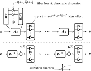
Figure 1: Block diagram of the split-step method to numerically solve the nonlinear Schrödinger equation (top) and the canonical model of a deep feed-forward neural network (bottom).

The parameter vector $\theta$ encapsulates all elements in the weight matrices and bias vectors, where we write $\theta=\{\bm{W}^{(1)},\dots,\bm{W}^{(m)},\bm{b}^{(1)},\dots,\bm{b}^{(m)}\}$ with some abuse of notation. NNs are universal function approximators, in the sense that they can approximate any desired function arbitrarily well by properly choosing the parameters $\theta$ and assuming a sufficiently large network architecture [44].

II-B Supervised Learning

In a supervised learning setting, one has a training set $S\subset{\mathcal{X}}\times{\mathcal{Y}}$ containing a list of input–output pairs that implicitly define a desired mapping. Then, training proceeds by minimizing the empirical training loss $\mathcal{L}_{S}(\theta)$, where the empirical loss $\mathcal{L}_{A}(\theta)$ for a finite set $A\subset{\mathcal{X}}\times{\mathcal{Y}}$ of input–output pairs is defined by

$$\mathcal{L}_{A}(\theta)\triangleq\frac{1}{|A|}\sum_{({\bm{x}},{\bm{y}})\in A}l\big{(}f_{\theta}({\bm{x}}),{\bm{y}}\big{)}$$ (2)

and $l({\hat{\bm{y}}},{\bm{y}})$ is the per-example loss function associated with returning the output ${\hat{\bm{y}}}=\bm{f}_{\theta}({\bm{x}})$ when ${\bm{y}}$ is correct. When the training set is large, the parameter vector $\theta$ is commonly optimized by using a variant of stochastic gradient descent (SGD). In particular, standard mini-batch SGD uses the parameter update

$$\theta_{t+1}=\theta_{t}-{\mu}\nabla\mathcal{L}_{B_{t}}(\theta_{t}),$$ (3)

where ${\mu}$ is the learning rate and $B_{t}\subseteq S$ is the mini-batch used in the $t$-th step. Typically, $B_{t}$ is chosen to be a random subset of $S$ with some fixed size that matches available computational resources, e.g., graphical processing units (GPUs).

Supervised learning is not restricted to NNs and learning algorithms such as SGD can be applied to other function classes as well. Indeed, in this paper, we do not use NNs, but instead exploit the underlying signal-propagation dynamics in optical fiber to construct a suitable model $\bm{f}_{\theta}$.

III Physics-Based Machine-Learning Models

Consider a complex-valued baseband signal $x(t)$, which is transmitted over an optical fiber as illustrated in Fig. 2. The signal propagates according to the NLSE [28, p. 40]

$$\frac{\partial u(z,t)}{\partial z}={-\frac{\alpha}{2}u(z,t)}-\jmath\frac{\beta_{2}}{2}\frac{\partial^{2}}{\partial t^{2}}u(z,t)+\jmath\gamma|u(z,t)|^{2}u(z,t),$$ (4)

where $u(z=0,t)\triangleq x(t)$, $\alpha$ is the loss parameter, $\beta_{2}$ is the CD coefficient, and $\gamma$ is the nonlinear Kerr parameter. The signal after propagation distance $L$ is denoted by $y(t)\triangleq u(z=L,t)$. Note that (4) covers single-polarization systems. The extension to dual-polarization transmission is discussed in Sec. III-D.

Figure 2: Conceptual signal evolution in a single-mode fiber. The nonlinear Schrödinger equation implicitly describes the relationship between the input signal $x(t)=u(z=0,t)$ and the output signal $y(t)=u(z=L,t)$.

III-A The Split-Step Method

In general, (4) does not admit a closed-form solution and must be solved using numerical methods. One of the most popular methods is the SSM which is typically implemented via block-wise processing of sampled (i.e., discrete-time) waveforms. To that end, assume that the signals $x(t)$ and $y(t)$ are sampled at $t=k/f_{\text{s}}$ to give sequences of samples $\{x_{k}\}_{k\in\mathbb{Z}}$ and $\{y_{k}\}_{k\in\mathbb{Z}}$, respectively. We further collect $n$ consecutive samples into the respective vectors $\bm{x}=(x_{1},\dots,x_{n})^{\top}$ and $\bm{y}=(y_{1},\dots,y_{n})^{\top}$, where $\bm{x},\bm{y}\in\mathbb{C}^{n}$. In order to derive the SSM, it is now instructive to consider the time-discretized NLSE

$$\frac{\mathrm{d}\bm{u}(z)}{\mathrm{d}z}={-\frac{\alpha}{2}\bm{u}(z)}+\bm{A}\bm{u}(z)+\jmath\gamma\bm{\rho}(\bm{u}(z)),$$ (5)

where $\bm{A}=\bm{F}^{-1}\operatorname{\text{diag}}(H_{1},\dots,H_{n})\bm{F}$, $\bm{F}$ is the $n\times n$ discrete Fourier transform (DFT) matrix, $H_{k}=\jmath\frac{\beta_{2}}{2}\omega_{k}^{2}$, $\omega_{k}=2\pi f_{k}$ is the $k$-th DFT angular frequency (i.e., $f_{k}/f_{\text{s}}=(k-1)/n$ if $k<n/2$ and $f_{k}/f_{\text{s}}=(k-1-n)/n$ if $k\geq n/2$), and $\bm{\rho}:\mathbb{C}^{n}\to\mathbb{C}^{n}$ is defined as the element-wise application of $\rho(x)=x|x|^{2}$. Eq. (5) is a first-order ordinary differential equation with a vector-valued function $\bm{u}(z)$, where $\bm{u}_{0}\triangleq\bm{u}(0)=\bm{x}$ is the initial boundary condition. Next, the fiber is conceptually divided into $M$ segments of lengths $\delta_{1},\ldots,\delta_{M}$ such that $\sum_{i=1}^{M}\delta_{i}=L$. It is then assumed that for sufficiently small $\delta_{i}$, the effects stemming from the linear and nonlinear terms on the right hand side of (5) can be separated. More precisely, for $\gamma=0$, (5) is linear with solution $\bm{u}(z)=\bm{A}_{z}\bm{u}_{0}$, where $\bm{A}_{z}\triangleq{e^{-\frac{\alpha}{2}z}}e^{z\bm{A}}$ and $e^{z\bm{A}}=\bm{F}^{-1}\operatorname{\text{diag}}(e^{zH_{1}},\dots,e^{zH_{n}})\bm{F}$. For $\alpha=0$ and $\beta_{2}=0$, one may verify that the solution is $\bm{u}(z)=\bm{\sigma}_{z}(\bm{u}_{0})$, where $\bm{\sigma}_{z}:\mathbb{C}^{n}\to\mathbb{C}^{n}$ is the element-wise application of $\sigma_{z}(x)=xe^{\jmath\gamma z|x|^{2}}$. Alternating between these two operators for $z=\delta_{i}$ leads to the SSM

$$\bm{u}_{i}=\bm{\sigma}_{\delta_{i}}\left(\bm{A}_{\delta_{i}}\bm{u}_{i-1}\right),\qquad i=1,2,\dots,M,$$ (6)

where $\bm{u}_{i}$ serves as an estimate $\bm{u}_{i}\approx\bm{u}(\delta_{1}+\dots+\delta_{i})$. We note that it is typically more accurate to also consider the effect of the loss term in the nonlinear step by using $\sigma_{z}(x)=xe^{\jmath\gamma{L_{\text{eff}}(z)}|x|^{2}}$ where $L_{\text{eff}}(z)=(1-e^{-\alpha z})/\alpha$ is the so-called effective nonlinear length. The corresponding block diagram for $\delta_{1}=\cdots=\delta_{M}=\delta$ is shown in the top of Fig. 1.

The degree to which ${\bm{u}_{M}}$ constitutes a good approximation of the sampled signal vector $\bm{y}=\bm{u}(L)$ (and therefore the true waveform $y(t)$ at distance $L$) is now a question of choosing $M$, $f_{\text{s}}$, and $n$. In practice, the sampling frequency $f_{\text{s}}$ and the number of steps $M$ are chosen to ensure sufficient temporal and spatial resolution, respectively. The block length $n$ can be chosen such that the overhead is minimized in overlap-and-save techniques for continuous data transmission.

III-B Parameterizing the Split-Step Method

From the side-by-side comparison in the top and bottom of Fig. 1, it is evident that the SSM has essentially the same functional form as a deep feed-forward NN; in both cases, one alternates between linear (or affine) steps and simple pointwise nonlinearities. The main idea in this paper is to exploit this observation by (i) appropriately parameterizing the SSM, and (ii) applying the obtained parameterized model instead of a generic NN.

Remark 1.

Conventional deep-learning tasks such as speech or object recognition are seemingly unrelated to nonlinear signal propagation over optical fiber. One may therefore wonder if the similarity to the SSM is merely a coincidence. In that regard, some authors argue that deep NNs perform well because their functional form matches the hierarchical or Markovian structure that is present in most real-world data [43]. Indeed, the SSM can be seen as a practical example where such a structure arises, i.e., by decomposing the physical process described by (4) into a hierarchy of elementary steps. Similar observations were made in [45], where the training of deep NNs is augmented by penalizing non-physical solutions.

Our parameterization of the SSM is directly inspired by the functional form of NNs. In particular, instead of using the matrix $\bm{A}_{\delta_{i}}$ in each of the $M$ steps, we propose to fully parameterize all linear steps by assuming general matrices $\bm{A}^{(1)},\dots,\bm{A}^{(\ell)}\in\mathbb{C}^{n\times n}$, similar to the weight matrices in a NN, where $\ell=M$ refers to the number of model steps (or layers). By combining the parameterized linear steps and the standard nonlinearities in the SSM, one obtains a parameterized version of the SSM according to

$$\bm{f}_{\theta}(\bm{x})=\bm{\sigma}_{\ell}(\bm{A}^{(\ell)}\dots\bm{\sigma}_{1}(\bm{A}^{(1)}\bm{x})),$$ (7)

where $\theta=\{\bm{A}^{(1)},\dots,\bm{A}^{(\ell)}\}$ collects all tunable parameters and we have defined $\bm{\sigma}_{i}\triangleq\bm{\sigma}_{\delta_{i}}$.

Remark 2.

The nonlinear operators can also be parameterized [29], e.g., by introducing scaling factors $\eta^{(1)},\dots,\eta^{(\ell)}\in\mathbb{R}$ according to $\sigma_{i}(x)=xe^{\jmath\eta^{(i)}\gamma{L_{\text{eff}}(\delta_{i})}|x|^{2}}$. However, it can be shown that this may lead to an overparameterized model, see Remark 4 below. In this paper, we do not consider this parameterization and assume fixed nonlinearities.

The above parameterization has the drawback that the number of parameters grows quadratically with the block length $n$. A more practical parameterization is obtained by constraining each matrix $\bm{A}^{(i)}$ to an equivalent (circular) convolution with a filter. In this paper, we restrict ourselves to finite impulse response (FIR) filters which are further constrained to be symmetric. In this case, all matrix rows are circularly-shifted versions of $(h^{(i)}_{K_{i}},\dots,h^{(i)}_{1},h^{(i)}_{0},h^{(i)}_{1},\dots,h^{(i)}_{K_{i}},0,\dots,0)$, where $h^{(i)}_{j}\in\mathbb{C}$, $j=-K_{i},\dots,K_{i}$, are the filter coefficients and $T_{i}=2K_{i}+1$ is the filter length. After collecting all tunable coefficients in a vector $\bm{h}^{(i)}\triangleq(h^{(i)}_{0},h^{(i)}_{1},\dots,h^{(i)}_{K_{i}})$, the new parameter vector for the entire model is $\theta=\{\bm{h}^{(1)},\dots,\bm{h}^{(\ell)}\}$. This reduces the number of real parameters per weight matrix from $2n^{2}$ to $2(K_{i}+1)$, where typically $K_{i}\ll n$. This restriction also implies that the resulting model is fully compatible with a time-domain filter implementation [46], where symmetric coefficients can be exploited by using a folded implementation. An example of the resulting DSP structure for $\ell=2$ steps with $T_{1}=5$ and $T_{2}=3$ is shown in Fig. 3.

Figure 3: DSP structure with folded FIR filters for $\ell=2$, $T_{1}=5$, and $T_{2}=3$. Triangles represent the (pointwise) nonlinear steps.

Remark 3.

It is worth pointing out that several problems that have been previously studied for the standard SSM can be regarded as special cases of the proposed model. For example, it is well known that non-uniform step sizes can improve accuracy [47], which leads to the problem of finding an optimized step-size distribution. Another common problem is to properly adjust the nonlinearity parameter in each step (i.e., using $\gamma^{\prime}$ instead of the actual fiber parameter $\gamma$) which is sometimes referred to as “placement” optimization of the nonlinear operator [33]. Since our model implements general linear steps, a step-size optimization can be thought of as being implicitly performed. Moreover, it can be shown that adjusting the nonlinearity parameters is equivalent to rescaling the filter coefficients in the linear steps, thereby adjusting the filter gain. Thus, a joint nonlinear operator placement can also be regarded as a special case. Indeed, the proposed model is more general and can learn and apply arbitrary filter shapes to the signal in a distributed fashion. This includes, e.g., low-pass filters, which have recently been shown to improve simulation accuracy [48].

III-C Generalization to other Split-Step Methods

We now discuss several generalizations of the model (7), focusing on other variants of the SSM.

The numerical method described in Sec. III-A corresponds to the so-called asymmetric version of the SSM. In practice, a symmetric version is typically used because it reduces the approximation error from $\mathcal{O}(M^{-1})$ to $\mathcal{O}(M^{-2})$ at almost no extra cost [28]. The symmetric SSM is defined by

$$\bm{u}_{i}=\bm{A}_{\delta_{i}/2}\bm{\sigma}_{\delta_{i}}\left(\bm{A}_{\delta_{i}/2}\bm{u}_{i-1}\right),\qquad i=1,2,\dots,M.$$ (8)

The model $\bm{f}_{\theta}$ in (7) can also be based on parameterizing the symmetric SSM, which was done in [29, 35]. In that case, the general form in (7) remains valid. The main difference is that $\ell=M+1$, i.e., an $\ell$-step model is based on the symmetric SSM with $\ell-1$ steps. The last model step only corresponds to a linear “half-step” without application of the nonlinear Kerr operator. This can be achieved by setting $\delta_{\ell}=0$, which gives $\sigma_{\ell}(x)=xe^{\jmath\gamma{L_{\text{eff}}(\delta_{\ell})}|x|^{2}}=x$ and thus $\bm{\sigma}_{\ell}(\bm{x})=\bm{x}$.

Remark 4.

For models based on the symmetric SSM, one can also show that introducing scaling factors in the nonlinear steps (as suggested in Remark 2) leads to an overparameterization, in the sense that the parameterization of the nonlinear operators via $\eta^{(1)},\dots,\eta^{(\ell)}$ is redundant. More precisely, consider the model $\bm{f}_{\theta}$ in (7) with parameterized nonlinear steps, i.e., $\theta=\{\bm{h}^{(1)},\dots,\bm{h}^{(\ell)},\eta^{(1)},\dots,\eta^{(\ell)}\}$ and assume that $\eta^{(\ell)}=0$. Then, there always exists $\tilde{\theta}=\{\tilde{\bm{h}}^{(1)},\dots,\tilde{\bm{h}}^{(\ell)},\tilde{\eta}^{(1)},\dots,\tilde{\eta}^{(\ell)}\}$ with $\tilde{\eta}^{(1)}=\cdots=\tilde{\eta}^{(\ell-1)}=1$ and $\tilde{\eta}^{(\ell)}=0$, such that $\bm{f}_{\theta}(\bm{x})=\bm{f}_{\tilde{\theta}}(\bm{x})$ for all $\bm{x}\in\mathbb{C}^{n}$. The proof is based on renormalizing the intermediate signals prior to the nonlinearities and absorbing the normalization constants into the filter coefficients.

Besides using the symmetric SSM, it can also be beneficial to filter the squared modulus of the signal prior to applying the nonlinear phase shift [33]. In the context of nonlinearity compensation, this approach is known as filtered (or low-pass filtered) DBP and variations of this idea have been explored in, e.g., [49, 50, 34]. We adopt the terminology from [34] and refer to the corresponding numerical method as the enhanced SSM (ESSM). The main difference with respect to the standard SSM is that the nonlinear steps are modified according to

$$[\bm{\sigma}_{z}(\bm{x})]_{j}=x_{j}e^{\jmath\gamma{L_{\text{eff}}(z)}\sum_{k=-\kappa}^{\kappa}\eta_{k}|x_{j-k}|^{2}},$$ (9)

where $[\bm{a}]_{j}=a_{j}$ returns the $j$-th entry of $\bm{a}$ and the indexing $x_{j-k}$ is interpreted modulo $n$. Compared to standard nonlinearities, the phase shift at time $j$ now also depends on the signal at other time instances through the filter $\bm{\eta}=(\eta_{-\kappa},\dots,\eta_{0},\dots,\eta_{\kappa})$, where the filter taps are assumed to be real-valued. We propose to generalize the ESSM by again parameterizing all steps according to

$$[\bm{\sigma}_{i}(\bm{x})]_{j}=x_{j}e^{\jmath\gamma{L_{\text{eff}}(z)}\sum_{k=-\kappa_{i}}^{\kappa_{i}}\eta_{k}^{(i)}|x_{j-k}|^{2}},$$ (10)

where $\bm{\eta}^{(i)}=(\eta_{-{\kappa_{i}}}^{(i)},\dots,\eta_{0}^{(i)},\dots,\eta_{\kappa_{i}}^{(i)})$, $i=1,\dots,\ell$, are different filters in each step. The optimization parameters then become $\theta=\{\bm{h}^{(1)},\dots,\bm{h}^{(M)},\bm{\eta}^{(1)},\dots,\bm{\eta}^{(M)}\}$. We demonstrate in Sec. V-C that such a parameterization indeed leads to improvements compared to prior work that uses the same filter $\bm{\eta}$ in each nonlinear step.

Lastly, there are other versions of the SSM where our approach could be applied. One example is the iterative SSM described in [28, Sec. 2.4.1]. This method falls into the class of predictor–corrector methods, where the corrector step is iterative. While we have not explored the parameterization of the iterative SSM in this work, the general idea is to “unroll” the iterations in order to obtain a proper feed-forward computation graph that can again be parameterized.

Remark 5.

Finite-difference methods have also be used extensively to solve the NLSE. In fact, they can be more computationally efficient than the SSM in some applications [28, 2.4.2]. However, to the best of our knowledge, finite-difference methods have not been studied for real-time applications such as DBP. One reason for this might be that many methods that show good performance are implicit, i.e., they require solving a system of equations at each step. This makes it challenging to satisfy a real-time constraint.

III-D Generalization to Dual-Polarization Systems

Our approach also generalizes beyond the standard NLSE in (4) to the case of coupled NLSEs. These arise, for example, in the context of subband processing, where we refer the interested reader to [36] for more details. Another important example is the generalization to dual-polarization systems. In this case, the signal evolution is described by a set of coupled NLSEs that takes into account the interactions between the two (degenerate) polarization modes. In birefringent fibers where polarization states change rapidly along the link, an appropriate approximation is given by the so-called Manakov-PMD equation [51]. Parameterizing the SSM for the Manakov-PMD equation was previously done in [37] (with early work briefly described in [52]) and also recently in [42]. In general, however, these generalizations lead to nontrivial choices for the specific parameterizations of the linear and nonlinear steps, and a detailed discussion is beyond the scope of this paper. Note for example that the parameterizations described in [37] and [42] are different and more research is needed to properly compare the performance of the resulting systems.

IV Application to Nonlinear Interference Mitigation: Learned Digital Backpropagation

As an application, we consider nonlinear equalization via receiver-side digital backpropagation (DBP) [53, 54, 55, 56], with an emphasis on a low-complexity hardware-efficient implementation. DBP exploits the fact that, in the absence of noise, the transmitted signal can be recovered by solving an initial value problem (IVP) using the received signal as a boundary condition [57]. In practice, the received signal first passes through an analog-to-digital converter and the IVP can then be solved approximately via receiver DSP. Here, we apply the parameterized SSM introduced in the last section and show how to optimize it using machine-learning tools. We refer to the resulting approach as learned DBP (LDBP).

A major issue with DBP is the large computational burden associated with a real-time DSP implementation. Thus, various techniques have been proposed to reduce its complexity [55, 58, 33, 59, 60, 49, 9, 50, 61, 10, 62, 34, 46, 63, 64, 65]. In essence, the task is to approximate the solution of a partial differential equation using as few computational resources as possible. We approach this problem from a machine-learning perspective by applying model compression, which is commonly used to reduce the size of NNs [66, 67]. As explained in detail below, we use a pruning-based approach, where the filters in the LDBP model are progressively shortened during SGD.

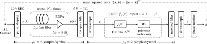
Figure 4: Block diagram showing the entire end-to-end system model.

IV-A System Model

A block diagram of the system model is shown in Fig. 4. The transmitted signal is given by

$$x(t)=\sqrt{P}\sum_{k=-\infty}^{\infty}s_{k}p\left(t-\frac{k}{{R_{\text{s}}}}\right),$$ (11)

where $P$ is the signal power, $\{s_{k}\}_{k\in\mathbb{Z}}$ is a sequence of complex symbols, $p(t)$ is the impulse response of a root-raised cosine (RRC) filter with $10\%$ roll-off factor, and ${R_{\text{s}}}$ is the baud rate. The symbol sequence is assumed to be periodic consisting of repeated versions of the vector $\bm{s}=(s_{1},\dots,s_{N_{\text{sym}}})\in\mathbb{C}^{N_{\text{sym}}}$. The symbols in $\bm{s}$ are independent and identically distributed (i.i.d.) circularly-symmetric complex Gaussian, and further normalized such that $\mathbb{E}[|S_{i}|^{2}]=1$. The signal $x(t)$ is assumed to be transmitted over an optical link consisting of $N_{\text{sp}}$ spans of standard single-mode fiber. Each span has length $L_{\text{sp}}$ and an erbium-doped fiber amplifier (EDFA) with noise figure $N_{\text{F}}$ is inserted after each span to compensate exactly for the incurred signal attenuation. Each EDFA introduces white Gaussian noise with power spectral density $(e^{\alpha L_{\text{sp}}}-1)h\nu_{s}n_{\text{sp}}$ [68, Eq. (54)], where $h$ is Planck’s constant, $\nu_{s}$ is the optical carrier frequency, and $n_{\text{sp}}=N_{\text{F}}(2(1-e^{-\alpha L_{\text{sp}}}))^{-1}$ is the spontaneous emission factor. After propagation distance $L=N_{\text{sp}}L_{\text{sp}}$, the received signal $y(t)$ is low-pass filtered using an ideal brick-wall filter with bandwidth $\Delta B=2f_{\text{s}}$ and sampled at $t=k/f_{\text{s}}$ to give a sequence of received samples $\{r_{k}\}_{k\in\mathbb{Z}}$, where $\rho_{\text{d}}=f_{\text{s}}/{R_{\text{s}}}$ is the digital oversampling factor. The first $n=\rho_{\text{d}}N_{\text{sym}}$ samples are collected into the observation vector $\bm{r}=(r_{1},\dots,r_{n})\in\mathbb{C}^{n}$. Forward propagation is simulated using $\rho_{\text{a}}>\rho_{\text{d}}$ samples/symbol.

The goal is to recover $\bm{s}$ from the observation $\bm{r}$. To that end, we use a receiver DSP chain that consists of three blocks: (i) LDBP, (ii) a digital matched filter (i.e., RRC filter with $10\%$ roll-off factor) followed by downsampling, and (iii) a phase-offset correction. LDBP alternates linear and nonlinear steps according to (7), as shown in Fig. 4. The phase-offset correction is performed according to $\hat{\bm{s}}=\tilde{\bm{s}}e^{-\jmath\hat{\phi}}$, where $\hat{\phi}=\arg(\bm{s}^{\dagger}\tilde{\bm{s}})$ and $\tilde{\bm{s}}$ is the symbol vector after the matched filter. The entire receiver DSP chain can then be written as

$$\hat{\bm{s}}=e^{-\jmath\hat{\phi}}\bm{M}\bm{f}_{\theta}(\bm{r}),$$ (12)

where $\bm{M}\in\mathbb{R}^{N_{\text{sym}}\times n}$ is a circulant matrix that represents the matched filter and downsampling by a factor $\rho_{\text{d}}$.

Remark 6.

Since the matched filter is linear, one could also include it in the LDBP model as a linear layer, as was done in [29]. Note that the phase-offset correction is genie-aided, in the sense that knowledge about the transmitted symbol vector is assumed. Alternatively, the phase-offset rotation could be included in the machine-learning model where $\hat{\phi}$ would then become an additional parameter. In this paper, these algorithms are instead applied as separate receiver DSP block after LDBP.

Remark 7.

Similar to comparable prior work on complexity-reduced DBP (e.g., [55, 33]), our system model does not include various hardware impairments and other imperfections that may arise in practice. However, it has been shown that LDBP can be successfully trained in the presence of such impairments. For example, [38, 39] propose a training method which is blind to timing error, state of polarization rotation, frequency offset, and phase offset. The approach works by first estimating these parameters using a conventional DSP chain and treating the corresponding compensation blocks as static layers during the training. Similar approaches were also proposed in [41, 42] to allow for the training with experimental data sets.

IV-B Joint Parameter Optimization

In order to optimize all parameters in $\theta$, supervised learning is applied as described in Sec. II-B. The training is performed using the Adam optimizer [69], which is a variant of SGD. The chosen loss function is the mean squared error (MSE) between the correct and estimated symbols, i.e., $l(\hat{\bm{s}},\bm{s})=\|\hat{\bm{s}}-\bm{s}\|^{2}/N_{\text{sym}}$, where $\|\bm{s}\|^{2}\triangleq\sum_{i=1}^{N_{\text{sym}}}|s_{i}|^{2}$. The empirical loss in (2) then becomes a Monte Carlo approximation of the expected MSE

$$\mathbb{E}\left[l(\hat{\bm{S}},\bm{S})\right]=\frac{1}{N_{\text{sym}}}\mathbb{E}\left[\|\hat{\bm{S}}-\bm{S}\|^{2}\right],$$ (13)

where the expectation is over the transmitted symbols and the noise generated by the optical amplifiers. Note that minimizing the MSE is equivalent to maximizing the effective SNR

$$\text{SNR}=N_{\text{sym}}\mathbb{E}\left[(\|\hat{\bm{S}}-\bm{S}\|^{2})^{-1}\right].$$ (14)

The effective SNR is used as the figure of merit for the numerical results presented in the next section.

For a fixed link setup, our numerical results show that the optimal parameter vector depends on the input power $P$. Thus, to achieve the best performance one needs to perform a separate optimization for each input power. In order to reduce the training time, we instead perform the optimization over a range of different input powers. More precisely, the particular input power for each transmitted frame is chosen uniformly at random from a discrete set of input powers $\mathcal{P}$. The set $\mathcal{P}$ is chosen based on the particular scenario. The power dependence of the learned solutions will be further investigated in Sec. V-D.

IV-C Parameter Initialization and Filter Pruning

Since SGD is a local search method, choosing a suitable parameter-initialization scheme is important to facilitate successful training. Our approach leverages the fact that the proposed model is based on a well-established numerical method by initializing the parameters such that the initial performance is close to the standard SSM. We also experimented with other initializations, see Sec. V-E.

Our parameter initialization starts by specifying the desired number of SSM steps and this changes the number of layers in the LDBP model. For the asymmetric SSM, the number of steps is directly equivalent to the number of layers, i.e., $\ell=M$. For the symmetric SSM, we have $\ell=M+1$ and the last model layer is a linear half-step without nonlinearity as described in Sec. III-C. To compute the step sizes for a given number of steps per span (StPS), the logarithmic heuristic in [70, Eq. (2)] is used with the recommended adjusting factor $0.4$. This leads to a set of step sizes $\delta_{1},\dots,\delta_{M}$. After combining adjacent half-steps, one obtains the lengths $\delta^{\prime}_{1},\dots,\delta^{\prime}_{\ell}$, which are then used for the filter initialization in each step.

Example 1.

For illustration purposes, let $L_{\text{sp}}=100$ km and $N_{\text{sp}}=2$, and assume that LDBP is based on the symmetric SSM with $2$ StPS. With these assumptions, the logarithmic step-size heuristic in [70] leads to $\delta_{1}=\delta_{3}\approx 70$ km and $\delta_{2}=\delta_{4}\approx 30\,$km. After combining adjacent half-steps, the LDBP model has $\ell=5$ layers and the equivalent step sizes to initialize the FIR filters are $\delta^{\prime}_{1}=35$ km, $\delta^{\prime}_{2}=\delta^{\prime}_{3}=\delta^{\prime}_{4}=50$ km, $\delta^{\prime}_{5}=15$ km. In this case, the initial filter coefficients for $\bm{h}^{(2)}$, $\bm{h}^{(3)}$, and $\bm{h}^{(4)}$ will be the same.  $\triangle$

Based on $\delta^{\prime}_{1},\dots,\delta^{\prime}_{M}$, a least-squares approach is then used for computing the initial filter coefficients. Recall that the ideal frequency response to invert CD over distance $\delta_{i}^{\prime}$ is $H(\omega)=e^{\jmath\xi\omega^{2}}$, where $\xi\triangleq-\beta_{2}\delta_{i}^{\prime}f_{\text{s}}^{2}/2$ and $\omega\triangleq 2\pi f/f_{\text{s}}$. Now, let $\mathcal{F}(\bm{h}^{(i)})=\sum_{k=-K_{i}}^{K_{i}}h_{k}^{(i)}e^{-\jmath k\omega}$ be the discrete-time Fourier transform of $\bm{h}^{(i)}$. The standard approach is to match $\mathcal{F}(\bm{h}^{(i)})$ to $e^{\jmath{\xi}\omega^{2}}$ by minimizing the frequency-response error. After discretizing the problem with $\omega_{i}=2\pi i/N$ for $i=-N/2,\dots,N/2$, one obtains $\min_{\bm{h}^{(i)}}\|\bm{B}\bm{h}^{(i)}-\bm{d}\|^{2}$, where $\bm{d}=(d_{-N/2},\dots,d_{0},\dots,d_{N/2})^{\top}$ with $d_{i}\triangleq e^{\jmath{\xi}\omega_{i}^{2}}$ and $\bm{B}$ is an $(N+1)\times T_{i}$ DFT matrix. In this paper, we use a variation proposed in [71], where the frequency-response error is minimized only within the signal bandwidth and the out-of-band filter gain is further constrained to be below some fixed maximum value, see [71] for more details. This procedure is applied for each of the $M$ filters.

In order to reduce the complexity of the final LDBP model, a simple pruning approach is applied where the filters are successively shortened during the gradient-descent optimization by forcing their outermost taps to zero. More precisely, we start with initial filter lengths $T_{1}^{\prime}>T_{1},\ldots,{T_{\ell}^{\prime}>T_{\ell}}$ which are chosen large enough to ensure good starting performance. The target lengths $T_{1},\dots,T_{\ell}$ implicitly define the filter taps that need to be removed. In our implementation, the affected taps are then multiplied with a binary mask, where all mask values are initially $1$. At certain predefined training iterations, some of the values are then changed to $0$, which effectively removes the corresponding filter taps from the model. Since all filters are assumed to be symmetric, the pruning is done such that each pruning step always removes the two outermost taps of a given filter (both having the same coefficient).

Example 2.

For the model in Example 1, assume that the initial filters have lengths $T_{1}^{\prime}=\cdots=T_{5}^{\prime}=11$ and that the target lengths are set to $T_{1}=\cdots=T_{5}=7$. Thus, the total number of pruning steps is $10$. Assuming, e.g., $100$ total SGD iterations, one filter is pruned every $10$ iterations, on average.  $\triangle$

The above approach does not take into account the importance of the filter taps before pruning them. Nonetheless, we found that it leads to both compact and well-performing models. Moreover, the final effective SNR is relatively insensitive to the pruning details (e.g., which filter tap is pruned in which iteration), as long as the pruning steps are sufficiently spread out and the target lengths $T_{i}$ are not too small. We also found empirically that it is generally beneficial to prune more taps in the beginning of the optimization procedure, rather than to spread out the pruning steps uniformly.

Remark 8.

In the machine-learning literature, pruning is commonly used to compress a large model (e.g., an image classifier) in order to facilitate deployment (e.g., on mobile devices). Similarly, our work shows that there exist compact solutions that could subsequently be deployed in a real-time DSP without performing any real-time optimization or pruning. We have previously studied LDBP from an ASIC implementation perspective in [35], where our particular design assumes that all tap coefficients are fully reconfigurable (but not trainable). Thus, in terms of operation in a real scenario, one option would be to train “offline” a set of different filter configurations for a variety of standard fiber parameters and propagation distances. Afterwards, an “online” testing phase could be used to identify the best-performing filters. To avoid large look-up tables and reduce the associated storage complexity, a conventional function approximator (e.g., a NN) could further be trained (also offline) to learn a smooth dependence between the system parameters (e.g., the fiber length) and the optimized filter coefficients. If more complexity is allowed, one could also try to explore the possibility of fine-tuning a subset of the filter coefficient via implementation of a real-time gradient-descent procedure. This would account for potential mismatches between the best pretrained filter coefficients and the actual optimal ones for the system under consideration. Assuming that the pretrained (i.e., already pruned) solutions provide good starting points for the optimization, no further real-time pruning would be required.

V Numerical Results

In this section, extensive numerical results are presented in order to verify the proposed approach. The numerical value of all system and training parameters can be found in Table I. The conventional asymmetric SSM with $500$ logarithmic StPS is used to simulate forward propagation. To estimate the effective SNR after training, we average over at least $10^{7}$ symbols.

TABLE I: List of symbols and system parameters.

symb.	parameter	comment / numerical value
$\alpha$	fiber loss parameter	$0.2$ dB/km
$\bm{b}^{(i)}$	NN bias vector
$\beta_{2}$	CD coefficient	$-21.683\,$ps2/km
$|\mathcal{B}_{t}|$	mini-batch size	$50$
$\Delta B$	low-pass bandwidth	$f_{\text{s}}$ ($37.5$ GHz in Fig. 9)
$\mathbb{C}$	set of complex numbers
$\delta_{i}/\delta_{i}^{\prime}$	SSM step sizes
$\mu$	learning rate (Adam)	$0.001$
$f_{\text{s}}$	sampling frequency	$\rho_{\text{d}}R_{\text{s}}$
$\mathcal{F}$	discrete-time Fourier trans.
$\gamma$	Kerr coefficient	$1.3$ rad/W/km
$h$	Planck’s constant	$6.626\cdot 10^{-34}$ Js
$\bm{h}^{(i)}$	LDBP filter coeffs.
$\bm{\eta}^{(i)}$	ESSM filter coeffs.
$\kappa/\kappa_{i}$	nonlinear filter param.	$20$ (Fig. 5)
$L_{\text{sp}}$	span length	$80\,$km (Figs. 5, 7), $100\,$km (Figs. 8, 9)
$l$	loss function	mean squared error (MSE)
$\ell$	total LDBP steps/layers	$4$, $25$ (Figs. 5, 7), $21$, $41$ (Figs. 8, 9)
$L$	transmission distance	$N_{\text{sp}}L_{\text{sp}}$
$L_{\text{eff}}$	eff. nonlinear length
$\mathcal{L}$	empirical loss
$M$	SSM steps	$500$ StPS (fwd. propagation)
$n$	samples per frame/block	$\rho_{\text{d}}N_{\text{sym}}$
$N_{\text{sp}}$	number of spans	$25$ (Figs. 5, 7), $10$ (Figs. 8, 9)
$N_{\text{sym}}$	symbols per frame	$1024$ (Figs. 5, 7, 8), $4096$ (Fig. 9)
$N_{\text{F}}$	noise figure	$5$ dB
$n_{\text{sp}}$	spont. emmission factor	$N_{\text{F}}(2(1-e^{-\alpha L_{\text{sp}}}))^{-1}$
$\nu_{s}$	carrier frequency	$1.946\cdot 10^{14}$ Hz
$P$	transmit power	$-12\,$dBm to $8\,$dBm
$\mathcal{P}$	power set for training	scenario-dependent (see text)
$p(t)$	pulse shape	root-raised cosine (10% roll-off)
$\rho_{\text{d}}$	digital oversampling	$2$
$\rho_{\text{a}}$	analog oversampling	$6$ (Figs. 5, 7, 8), $10$ (Fig. 9)
$\rho/\bm{\rho}$	nonlinearity	time-discretized NLSE (5)
$R_{\text{s}}$	symbol rate	$10.7$ Gbd (Figs. 5, 7), $32$ Gbd (Figs. 8, 9)
$\bm{r}$	observation vector
$\mathbb{R}$	set of real numbers
$\bm{s}$	i.i.d. symbol vector	Gaussian (except Fig. 7(b))
$\hat{\bm{s}}$	estimated symbol vector
$\tilde{\bm{s}}$	symbol vector after MF
$\sigma_{i}/\bm{\sigma}_{i}$	LDBP nonlinearity	$\bm{\sigma}_{i}=\bm{\sigma}_{\delta_{i}}$ (SSM nonlinearity)
$T_{i}^{\prime}$	filter len. before pruning	scenario-dependent (see text)
$T_{i}$	filter len. after pruning	scenario-dependent (see text)
$\theta$	parameter vector
$u/\bm{u}$	optical signal
$\bm{W}^{(i)}$	NN weight matrices
$\omega/\omega_{k}$	angular frequency
$\xi$	scaled CD coeff.	$-\beta_{2}\delta_{i}^{\prime}f_{\text{s}}^{2}/2$
$x(t)$	transmitted signal
$y(t)$	received signal
$\mathbb{Z}$	set of integers

V-A Revisiting Ip and Kahn, 2008

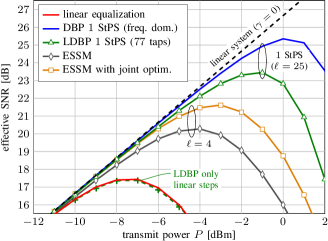
Figure 5: Results for $10.7\,$Gbaud over $25\times 80\,$km fiber (similar to [55]).

We start by revisiting [55], which considers single-channel transmission of a $10.7$-Gbaud signal over $25\times 80\,$km fiber. For this scenario, LDBP is based on the asymmetric SSM with $1$ StPS, i.e., $\ell=25$, and pruning is performed over $150,000$ gradient-descent iterations such that the final model alternates $5$-tap and $3$-tap filters, where initially $T_{i}^{\prime}=9$ for all $i$. The achieved effective SNR after training with $\mathcal{P}=\{-2,-1,0,1\}\,$dBm is shown in Fig. 5 by the green triangles. As a reference, the performance of linear equalization (red) and standard $1$-StPS DBP using frequency-domain filtering (blue) are shown. LDBP achieves a peak SNR of $23.5\,$dB using an overall impulse response length (defined as the length of the filter obtained by convolving all subfilters) of $13\cdot 4+12\cdot 2+1=77$ total taps. The peak-SNR penalty compared to DBP is around $2\,$dB, which allows us to directly compare to the results presented in [55]. Indeed, [55] also considers filter design for $1$-StPS DBP with the intention of quantifying the complexity overhead compared to linear equalization assuming real-time processing. Their filter design is based on frequency-domain sampling and the same filter is used in each step. With these assumptions, it was shown that $70$ taps/step are required to achieve performance within $2\,$dB of frequency-domain DBP—over $20$ times more than the number of taps required by LDBP.

V-B Performance–Complexity Trade-off

To further put the above results into perspective, we perform a similar complexity analysis as in [55], using real multiplications (RMs) as a surrogate. For the nonlinear steps, the exponential function is assumed to be implemented with a look-up table. It then remains to square each sample ($2$ RMs), multiply by $\gamma_{i}$ ($1$ RM), and compute the phase rotation ($4$ RMs). This gives $25\cdot 7=175$ RMs per sample. For the linear steps, one has to account for $13$ filters with $5$ taps and $12$ filters with $3$ taps. All filters have symmetric coefficients and can be be implemented using a folded structure with $h_{0}$-normalization as shown in [30, Fig. 5]. This gives $39\cdot 4=156$ RMs per sample. In comparison, the fractionally-spaced linear equalizer in [55] requires $188$ RMs per data symbol operating at $3/2$ samples/symbol. Thus, LDBP requires $3.5$ times more RMs per symbol. For the same oversampling factor as LDBP, a linear equalizer requires around $69$ taps (see below). This leads to $35\cdot 4=140$ RMs with a folded implementation and a complexity overhead for LDBP of only around $2$. If the linear equalizer is implemented in the frequency domain, the number of RMs is reduced to $n(4\log_{2}n+4)/(n-69)\approx 50$ per sample (see, e.g., [34, Sec. 4]), which increases the estimated complexity overhead factor to $6$. Still, these estimates are orders of magnitude lower than the complexity overhead in [55], which was estimated to be over $100$. For a more accurate estimation of the required hardware complexity, we refer the interested reader to [35], where LDBP is studied from an ASIC implementation perspective including finite-precision aspects.

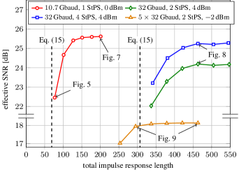
Figure 6: Performance as a function of the total LDBP impulse response length.

In general, the complexity of the linear steps scales directly with the number of filter taps. The red line in Fig. 6 shows the effective SNR of LDBP at $P=0\,$dBm as a function of the overall impulse response length at various levels of pruning. The right-most point of the curve corresponds to $T_{i}=T_{i}^{\prime}=9$ for all $i$, i.e., no pruning. To generate each curve in Fig. 6, we progressively prune the model for a total of $150,000$ gradient-descent iterations, and save the partially pruned model after every $25,000$ iterations. It can be seen that by allowing more than $77$ total taps, performance quickly increases up to around $25.5\,$dB, which is slightly higher than frequency-domain DBP, see Fig. 5. As a reference, the dashed line in Fig. 6 indicates the required number of filter taps that can be expected based on the memory that is introduced by CD. To estimate the memory, one may use the fact that CD leads to a group delay difference of $2\pi|\beta_{2}|\Delta fL$ over bandwidth $\Delta f$ and transmission distance $L$. Normalizing by the sampling interval $f_{\text{s}}^{-1}$, this confines the memory to approximately

$$T_{\text{cd}}=2\pi\beta_{2}\Delta fLf_{\text{s}}$$ (15)

samples. The bandwidth $\Delta f$ depends on the baud rate, the pulse shaping filter and the amount of spectral broadening. For a conservative estimate, we use $\Delta f=(1+0.1)\cdot 10.7\,$GHz (i.e., spectral broadening is ignored) which leads to $T_{\text{cd}}\approx 69$.

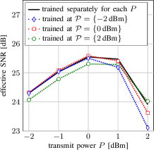
(a)

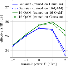
(b)

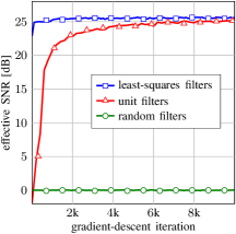
(c)

Figure 7: Additional results for $10.7\,$Gbaud over $25\times 80\,$km fiber: (a) power dependence, (b) modulation-format dependence, (c) parameter-initialization schemes.

V-C Improving the Enhanced SSM (Filtered DBP)

We now consider the ESSM which includes filters in the nonlinear steps. We start with the conventional ESSM, where a single filter is optimized (starting from a unit filter) and then applied in each step. Excluding the overhead due to overlap-and-save techniques, one ESSM step requires $4\log_{2}n+11+\kappa$ RMs per sample [34, Sec. 4, single pol.], where we recall that $2\kappa+1$ is the length of the filter in the nonlinear steps. We perform $4$ steps with $\kappa=20$, which gives roughly the same number of RMs as the $77$-tap LDBP model. The performance after training for $5000$ iterations is shown by the grey diamonds in Fig. 5. The ESSM achieves a smaller peak SNR by around $3\,$dB compared to LDBP, highlighting the advantage of using more steps. With the proposed modification of jointly optimizing all filters and assuming the same filter length as before (i.e., $\kappa_{1}=\ldots=\kappa_{4}=20$), more than $1\,$dB performance improvements over the conventional ESSM can be obtained for the same number of training iterations (yellow squares in Fig. 5).

V-D Generalization Error

Next, we study to what extend the learned solutions generalize beyond the training data, focusing on the transmit power and the employed modulation format. To do this efficiently, we consider the same setup as before, albeit using longer filters ($9$ taps/step) and without performing any pruning. In all cases, we train for $1500$ iterations. Fig. 7 (a) shows the performance after training separately for each input power $P$ (solid black line), compared to the case where training is performed at a specific power and the learned solution is then used at the other powers without retraining. From these results, it is clear that the optimal parameters are power-dependent in general and that the generalization error increases with the distance between the training and testing power. As mentioned in Sec. IV-B, our general approach to achieve a compromise between performance and training time is to optimize over a set of powers $\mathcal{P}$. The set $\mathcal{P}$ corresponds approximately to the power region where the performance peak (in terms of effective SNR) is expected. It is important to stress, however, that training over a large power range is not recommended, since the loss function in this case is dominated by regions with low effective SNR (i.e., large MSE).

Fig. 7 (b) shows the case where the modulation format differs between training and testing. Here, we consider the case where training is performed with Gaussian symbols and the solution is applied to $16$-QAM (and vice versa). In this case, LDBP appears to generalize well beyond the training data, especially in the linear operating regime.

V-E Parameter Initialization

As explained in Sec. IV-C, the filter coefficients are carefully initialized using least-squares fitting to the (per-step) inverse CD response. In general, we found that the chosen parameter initialization plays a critical role in determining the optimization behavior. To illustrate this, Fig. 7 (c) shows the learning curves obtained for the same scenario as in Sec. V-D, trained at $\mathcal{P}=\{0\,\text{dBm}\}$ with three different initialization schemes: least-squares filters, unit filters, and random filters. For the random case, the real and imaginary part of all taps are i.i.d. $\mathcal{N}(0,1)$. All filters are then normalized according to $\bm{h}^{(i)}\leftarrow\bm{h}^{(i)}/\sum_{j=-T_{i}}^{T_{i}}|h_{j}^{(i)}|^{2}$ for $i=1,\ldots,M$, which avoids numerical instabilities. However, the optimization remains essentially “stuck” at $0\,$dBm without improvements, suggesting the existence of a barrier in the optimization landscape that is difficult to overcome. This is somewhat surprising, given the fact that Gaussian initialization is widely used in the machine-learning literature. Unit filters converge to a reasonable SNR, albeit at a much slower convergence speed than the least-squares filters. Even though the final SNR after $10$k iterations is not quite competitive ($25.1\,$dB vs. $25.6\,$dB for least squares), this initialization has the advantage of being agnostic to the link setup, i.e., it does not require knowledge about parameters such as the fiber length or the dispersion coefficient.

V-F Higher Baud Rates

We now move on to higher baud rates and consider single-channel transmission of $32\,$Gbaud over $10\times 100\,$km of fiber. For this case, LDBP is based on the symmetric SSM with logarithmic step sizes. We use $2$ StPS and $4$ StPS, leading to $\ell=21$ and $\ell=41$, respectively. We start by investigating the number of filter taps required to achieve good performance. Results for $\mathcal{P}=\{4\,\text{dBm}\}$ are shown in Fig. 6 by the green ($2$ StPS) and blue ($4$ StPS) lines, assuming again $150,000$ total iterations and saving the partially pruned models after every $25,000$ iterations. As a reference, (15) with $\Delta f=(1+0.1)\cdot 32\,$GHz, $L=1000\,$km, and $f_{\text{s}}=64\,$GHz gives $T_{\text{cd}}=307$ taps, which is shown by the dashed line. Similar to before, the performance drops sharply when the filters are pruned too much and the impulse response length approaches the CD memory. For comparison, we note that Martins et al. consider filter design (and quantization) for time-domain DBP assuming $32\,$Gbaud signals in [32]. Their filters require $301$ taps to account for one span of $108\,$km fiber. Extrapolating to $L=1000\,$km and adjusting for the slighty increased dispersion parameter in [32] ($20.17\,$ ps/nm/km vs $17\,$ ps/nm/km), the total number of taps would be around $301\cdot 1000/108\cdot 17/20.17\approx 2350$ which is significantly larger than the results in Fig. 6.

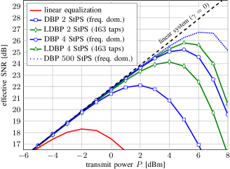
Figure 8: Results for $32\,$Gbaud over $10\times 100\,$km fiber

Another interesting observation from Fig. 6 is that for the same performance, the model with more steps requires fewer total taps, and hence less complexity to implement all linear steps. This is interesting because it is commonly assumed that the complexity of the SSM/DBP simply scales lineary with the number of steps, leading to an undesirable complexity increase. On the other hand, our results show that by carefully optimizing and pruning the linear steps, a very different complexity scaling can be achieved. Indeed, doubling the number of steps reduces the expected CD memory per step in half, which allows us to decrease the per-step complexity by reducing the filter lengths (ideally by half). The additional performance gain due the larger step count can then be traded off for fewer taps, as shown in Fig. 6.

Fig. 8 shows the performance of the two LDBP models with $463$ taps as a function of transmit power, where we retrain the solutions obtained in Fig. 8 with $\mathcal{P}=\{3,4,5\}\,$dBm ($2$ StPS) and $\mathcal{P}=\{4,5,6\}\,$dBm ($4$ StPS) for an additional $1500$ steps. Significant performance improvements are obtained compared to DBP with the the same number of StPS. In particular, the peak SNR is increased by $2.1\,$dB ($2$ StPS) and $0.6\,$dB ($4$ StPS), respectively. In the light of Remark 3, we conjecture that the gains can be partially attributed to the implicit joint optimization of step sizes and nonlinear operator placements.

V-G Wavelength Division Multiplexing

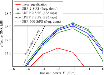
Figure 9: Results for $5\times 32\,$Gbaud (WDM) over $10\times 100\,$km fiber

Lastly, we study WDM transmissions, where it is known that the potential performance gains provided by static single-channel equalizers are limited due to nonlinear interference from neighboring channels, see, e.g., [72]. On the other hand, the resulting accuracy requirements for solving the NLSE are significantly relaxed compared to single-channel transmission because of the lower achievable effective SNRs. This provides an opportunity to further reduce complexity of LDBP by pruning additional filter taps. To demonstrate this, we consider $5\times 32\,$Gbaud WDM channels, where the channel spacing is $37.5\,$GHz. Compared to before, the receiver low-pass bandwidth is reduced to $\Delta B=37.5\,$GHz to filter out the center channel and the oversampling factor to simulate forward propagation as well as the number of symbols per block are increased to $\rho_{\text{a}}=10$ samples/symbols and $N_{\text{sym}}=4096$, respectively. Fig. 9 shows the performance of the $2$-StPS LDBP model with $463$ taps from Fig. 8, retrained for this scenario with $\mathcal{P}=\{-3,-2,-1\}\,$dBm (green diamonds) for $1500$ steps. This model already outperforms “ideal” DBP with $500$ StPS and increasing the number of steps or taps does not lead to significant improvements. On the other hand, further pruning the model by $36$% to $295$ taps only gave a peak-SNR penalty of around $0.2\,$dB (green circles), see also the yellow triangles in Fig. 6.

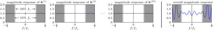
(a) Conventional approach

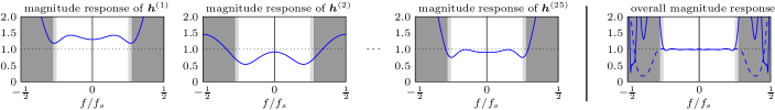
(b) Learned approach

Figure 10: Per-step filter responses (left) and overall filter response (right) for the simulation scenario in [55] at $P=-1\,$dBm, see Sec. V-A.

VI Examining The Learned Solutions

In this section, some of the obtained numerical results will be examined in more detail with a focus on the question “What can be learned from the resulting systems?”. Our goal is to explain why the filters in LDBP can be pruned to such short lengths compared to prior work, while still maintaining good performance. Indeed, we were pleasantly surprised that the machine-learning approach uncovered a simple but effective design strategy that had not been considered earlier. We also provide additional theoretical justifications and interpretations for the learned parameter configurations.

VI-A Conventional Filter Design for Digital Backpropagation

Filter design for the SSM has been considered in multiple prior works, both for enabling real-time DBP [55, 73, 74, 46, 63, 65, 32] and as a means to lower the simulation time of the forward propagation process [75, 76, 77]. The standard filter-design approach is to optimize a single filter and then use it repeatedly in each step. To compute the individual filter coefficients, a wide variety of approaches have been proposed. For instance, since the inverse Fourier transform of the CD response $H(\omega)=e^{\jmath\xi\omega^{2}}$ can be computed analytically, filter coefficients may be obtained through direct sampling and truncation [78]. Other approaches include frequency-domain sampling [55], wavelets [74], truncating the inverse DFT response [29], and least squares [79, 71]. However, all of these methods invariably introduce a truncation error due to the finite number of taps. Since repeating the same filter $M$ times raises the frequency response to the $M$-th power, the standard filter-design approach therefore leads to a coherent accumulation of truncation errors. In essence, using the same filter many times in series magnifies any weakness. To illustrate this, Fig. 10 (a) shows an example of the per-step responses (left) and overall response (right) for the $10.7\,$Gbaud scenario, where a standard least-squares fitting with $15$ taps/step is used. While the individual responses are relatively frequency-flat over the signal bandwidth, the overall response exhibits severe truncation errors.

The problem associated with applying the same filter multiple times in succession is of course well known and recognized in the literature. In fact, when commenting on their results in the book chapter [80], the authors explicitly state that the $70$ taps required for the filters in [55] are “much larger than expected”. They use the term “amplitude ringing” in order to explain this result: “Since backpropagation requires multiple iterations of the linear filter, amplitude distortion due to ringing accumulates” [80] (emphasis by us). The “requirement” mentioned in [55] to repeat the same filter seems to have implicitly guided almost all prior work on filter design for DBP. A notable exception is [73], where a complementary filter pair is optimized, rather than just one filter. While this does lead to improvements, one may argue that using the same filter pair multiple times in succession is again suboptimal and leads to the same “amplitude ringing” problem.

VI-B Learned Filter Responses

The learned per-step filter responses for the LDBP model alternating $5$-tap and $3$-tap filters (see Fig. 5) are shown in the left of Fig. 10 (b). At first glance, they may appear somewhat counterintuitive because these responses are generally much worse approximations to the “ideal” frequency-flat CD response, especially when compared to the filters obtained by least-squares fitting shown in Fig. 10 (a). On the other hand, when inspecting the overall magnitude response shown in the right of Fig. 10 (b), a rather different picture emerges. Indeed, the combined response follows an almost perfectly frequency-flat behavior. Another interesting observation is related to the fact that the learned overall response appears to exhibit a gain in the spectral region corresponding to the excess bandwidth of the pulse-shaping filter, i.e., the region between $50$% and $55$% of $f_{\text{s}}$, shaded in light gray. One may therefore wonder if this gain is of any significance, e.g., in terms of performance. Here, we argue instead that the learned approach has identified this spectral region as less important for the filter design, in the sense that a potentially larger truncation error can be tolerated because this region does not contain much of the signal power. Indeed, if one allows for more filter taps ($9$ taps, dashed line), the learned overall response becomes flat also in this region.

The machine-learning approach demonstrates that a precise approximation of the exact CD response in each step is not necessary for achieving good performance and that sacrificing individual filter accuracy can lead to a much better overall response. A theoretical justification for this observation can be obtained by regarding the filter-design problem for DBP as a multi-objective optimization problem. More precisely, instead of the standard least-squares formulation where only individual responses are optimized to fit the CD response, additional objectives should formulated based on the combined responses of neighboring filters, and in particular the overall response. In order to formalize this, consider the set of objectives

$$\mathcal{F}(\bm{h}^{(i)}) \circeq e^{\jmath\xi\omega^{2}}, i=1,2,\dots,M$$ (16)

$$\mathcal{F}(\bm{h}^{(i)}*\bm{h}^{(i+1)}) \circeq e^{\jmath 2\xi\omega^{2}}, i=1,2,\dots,M-1$$

$$\,\,\,\vdots$$

$$\mathcal{F}(\bm{h}^{(1)}*\cdots*\bm{h}^{(M)}) \circeq e^{\jmath M\xi\omega^{2}},$$

where the symbol $\circeq$ may be interpreted as “should be close to”. The conventional filter-design approach only utilizes the first objective based on the individual responses, in which case one finds that all filters should be the same. However, it can be shown that better filters are obtained by solving an optimization problem that targets all of the above objectives. In particular, keeping the coefficients for all but one filter constant, (16) can be written as a standard weighted LS problem as follows. Since, e.g., $\mathcal{F}(\bm{h}^{(i)}*\bm{h}^{(i+1)})=\mathcal{F}(\bm{h}^{(i)})\mathcal{F}(\bm{h}^{(i+1)})$, we have $(\bm{B}\bm{h}^{(i)})\circ(\bm{B}\bm{h}^{(i+1)})$ in the discretized problem, where $\circ$ denotes element-wise multiplication. Hence, one obtains

$$\min_{\bm{h}^{(i)}}\sum_{j=1}^{O_{i}}\lambda_{j}\|(\bm{B}\bm{h}^{(i)})\circ\bm{e}_{j}-\bm{d}_{j}\|^{2},$$ (17)

where $O_{i}$ is the number of objectives, $\lambda_{j}>0$ are weights, $\bm{e}_{j}$ are constant vectors representing the influence of other filters and $\bm{d}_{j}$ are the discretized objective vectors. This suggests a simple strategy for the joint filter optimization by solving the weighted LS problem for each of the $M$ filters in an iterative fashion. The weights $\lambda_{1},\dots,\lambda_{O_{i}}$ can be chosen based on a suitable system criterion, e.g., effective SNR. In [30], this approach was used to find better initializations compared to the filter truncation method used in [29]. While this approach does give improvements, it is not recommended anymore and we instead observe consistently better results by using the pruning approach described in Sec. IV-C. Nonetheless, we believe that the above formulation as a multi-objective optimization provides valuable insights into the filter-design problem.

Lastly, we point out that the performance when using only the linear steps in LDBP after training reverts approximately to that of a linear equalizer, as shown by the dotted green line (crosses) in Fig. 5. This leads to another intuitive interpretation of the task that is accomplished by deep learning. In particular, the optimized filter coefficients represent an approximate factorization of the overall linear inverse fiber response. At first, this may seem trivial because the linear matrix operator $e^{L\bm{A}}$ can be factored as $e^{\delta\bm{A}}\cdot\dots\cdot e^{\delta\bm{A}}$ with $L=\delta M$ for arbitrary $M$ to represent shorter propagation distances. However, the factorization task becomes nontrivial if we also require the individual operators $e^{\delta\bm{A}}$ to be “cheap”, i.e., implementable using short filters.

Remark 9.

A natural framework to study the factorization of FIR filters is via their $z$-transform. Recall that the $z$-transform of a symmetric FIR filter with $T$ taps is

$$H(z)=\sum_{n=0}^{T-1}h_{n}z^{-n}.$$ (18)

The polynomial $H(z)$ can be factorized according to

$$H(z)=h_{T-1}\prod_{i=1}^{T-1}(z^{-1}-q_{i}),$$ (19)

where $q_{i}$ is the $i$-th root of $H(z)$. This factorization can be interpreted as splitting the original filter into a cascade of $(T-1)/2$ symmetric $3$-tap filters. Note that while this splitting is exact, it is not unique, in the sense that the individual $3$-tap filters can be arbitrarily rescaled while preserving the overall filter gain (e.g., multiplying all coefficients of the first filter by $2$ and dividing all coefficient of any other filter by $2$ gives the same overall response). We experimented with this factorization based on the impulse response of a linear time-domain equalizer for the entire propagation distance. However, this approach gives no control over the individual filter responses, other than the choice of how to distribute the overall gain factor. Moreover, it is not obvious how to achieve a good ordering of sub-filters in the SSM.

VII Conclusions and Future Work

We have proposed a novel machine-learning approach for fiber-optic communication systems based on parameterizing the split-step method for the nonlinear Schrödinger equation. The resulting physics-based model was shown to have a similar mathematical structure compared to standard deep neural networks. It also comes with several compelling advantages:

• Clear hyperparameter choices: A major issue with standard NN models is the absence of clear guidelines for the network design, e.g., choosing the number of layers or the activation function. Our approach is based on a well-known numerical method where the “activation function” corresponds to the Kerr effect and one can leverage prior domain knowledge for selecting hyperparameters, specifically for choosing an appropriate number of layers.

• Good parameter initializations: Deep learning relies on local search methods, i.e., gradient descent. In general, it is nontrivial to find parameter-initialization schemes that facilitate successful training and allow for a reliable convergence to a good solution. For the proposed model, it was shown that good starting points for the optimization can be obtained by initializing parameters close to the standard split-step method.

• Model Interpretability: While neural networks are universal function approximators, it can be difficult to understand their inner workings and interpret the learned parameter configurations. On the other hand, the proposed model is based on familiar building blocks—FIR filters—where the learned frequency responses can reveal new theoretical insights into the obtained solutions.

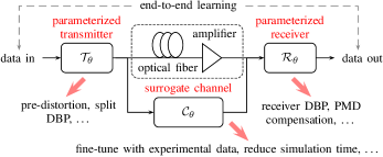
Figure 11: Potential applications of the proposed approach in the context of end-to-end autoencoder learning [8]. $\mathcal{T}_{\theta},\mathcal{R}_{\theta},\mathcal{C}_{\theta}$ are parameterized functions.

For future work, we note that while digital backpropagation is now most often used at the receiver, it was first studied as a transmitter pre-distortion technique [81, 82]. Therefore, besides receiver-side equalization, other potentially interesting applications include the learning of transmitter signaling schemes, or the optimization of both transmitter and receiver models similar to split nonlinearity compensation [83], see Fig. 11. The joint optimization of parameterized transmitters and receivers would also connect our work to the recently proposed end-to-end autoencoder learning approach in [8]. In general, this approach requires a differentiable channel model in order to compute gradients for the transmitter optimization. Since the proposed machine-learning model is based on the NLSE (and thus on the optical fiber channel), it can also serve as the basis for a fine-tuned surrogate channel, e.g., based on experimental data using techniques similar to [84, 85].

References

- [1] Y. LeCun, Y. Bengio, and G. Hinton, “Deep learning,” Nature, vol. 521, no. 7553, pp. 436–444, May 2015.
- [2] I. Goodfellow, Y. Bengio, and A. Courville, Deep Learning, 1st ed. MIT Press, 2016.
- [3] D. Zibar, M. Piels, R. Jones, and C. G. Schaeffer, “Machine learning techniques in optical communication,” J. Lightw. Technol., vol. 34, no. 6, pp. 1442–1452, Mar. 2016.
- [4] T. Wang, C. K. Wen, H. Wang, F. Gao, T. Jiang, and S. Jin, “Deep learning for wireless physical layer: Opportunities and challenges,” China Communications, vol. 14, no. 11, pp. 92–111, Nov. 2017.
- [5] O. Simeone, “A very brief introduction to machine learning with applications to communication systems,” IEEE Trans. Cogn. Commun. Netw., vol. 4, no. 4, pp. 648–664, Dec. 2018.
- [6] F. N. Khan, Q. Fan, C. Lu, and A. P. T. Lau, “An optical communication’s perspective on machine learning and its applications,” J. Lightw. Technol., vol. 37, no. 2, pp. 493–516, Jan. 2019.
- [7] M. Ibnkahla, “Applications of neural networks to digital communications - a survey,” Signal Process., vol. 80, no. 7, pp. 1185–1215, 2000.
- [8] T. O’Shea and J. Hoydis, “An introduction to deep learning for the physical layer,” IEEE Trans. Cogn. Commun. Netw., vol. 3, no. 4, pp. 563–575, Dec. 2017.
- [9] T. Shen and A. Lau, “Fiber nonlinearity compensation using extreme learning machine for DSP-based coherent communication systems,” in Proc. Optoelectronics and Communications Conf. (OECC), Kaohsiung, Taiwan, 2011.
- [10] A. M. Jarajreh, E. Giacoumidis, I. Aldaya, S. T. Le, A. Tsokanos, Z. Ghassemlooy, and N. J. Doran, “Artificial neural network nonlinear equalizer for coherent optical OFDM,” IEEE Photon. Technol. Lett., vol. 27, no. 4, pp. 387–390, Feb. 2015.
- [11] S. Gaiarin, X. Pang, O. Ozolins, R. T. Jones, E. P. Da Silva, R. Schatz, U. Westergren, S. Popov, G. Jacobsen, and D. Zibar, “High speed PAM-8 optical interconnects with digital equalization based on neural network,” in Proc. Asia Communications and Photonics Conf. (ACP), Wuhan, China, 2016.
- [12] S. T. Ahmad and K. P. Kumar, “Radial basis function neural network nonlinear equalizer for 16-QAM coherent optical OFDM,” IEEE Photon. Technol. Lett., vol. 28, no. 22, pp. 2507–2510, Nov. 2016.
- [13] J. Estarán, R. Rios-Müller, M. A. Mestre, F. Jorge, H. Mardoyan, A. Konczykowska, J. Y. Dupuy, and S. Bigo, “Artificial neural networks for linear and non-linear impairment mitigation in high-baudrate IM/DD systems,” in Proc. European Conf. Optical Communication (ECOC), Düsseldorf, Germany, 2016.
- [14] T. A. Eriksson, H. Bülow, and A. Leven, “Applying neural networks in optical communication systems: Possible pitfalls,” IEEE Photon. Technol. Lett., vol. 29, no. 23, pp. 2091–2094, Dec. 2017.
- [15] V. Kamalov, L. Jovanovski, V. Vusirikala, S. Zhang, F. Yaman, K. Nakamura, T. Inoue, E. Mateo, and Y. Inada, “Evolution from 8QAM live traffic to PS 64-QAM with neural-network based nonlinearity compensation on 11000 km open subsea cable,” in Proc. Optical Fiber Communication Conf. (OFC), San Diego, CA, 2018.
- [16] S. Li, C. Häger, N. Garcia, and H. Wymeersch, “Achievable information rates for nonlinear fiber communication via end-to-end autoencoder learning,” in Proc. European Conf. Optical Communication (ECOC), Rome, Italy, 2018.
- [17] R. T. Jones, T. A. Eriksson, M. P. Yankov, and D. Zibar, “Deep learning of geometric constellation shaping including fiber nonlinearities,” in Proc. European Conf. Optical Communication (ECOC), Rome, Italy, 2018.
- [18] B. Karanov, M. Chagnon, F. Thouin, T. A. Eriksson, H. Bulow, D. Lavery, P. Bayvel, and L. Schmalen, “End-to-end deep learning of optical fiber communications,” J. Lightw. Technol., vol. 36, no. 20, pp. 4843–4855, Oct. 2018.
- [19] B. Karanov, D. Lavery, P. Bayvel, and L. Schmalen, “End-to-end optimized transmission over dispersive intensity-modulated channels using bidirectional recurrent neural networks,” Opt. Express, vol. 27, no. 14, pp. 19 650–19 663, Jul. 2019.
- [20] R. T. Jones, M. P. Yankov, and D. Zibar, “End-to-end learning for GMI optimized geometric constellation shape,” in Proc. European Conf. Optical Communication (ECOC), Dublin, Ireland, 2019.
- [21] J. Song, B. Peng, C. Häger, H. Wymeersch, and A. Sahai, “Learning physical-layer communication with quantized feedback,” IEEE Trans. Commun., vol. 68, no. 1, pp. 645–653, Jan. 2020.
- [22] E. Nachmani, E. Marciano, L. Lugosch, W. J. Gross, D. Burshtein, and Y. Be’ery, “Deep learning methods for improved decoding of linear codes,” IEEE J. Sel. Topics Signal Proc., vol. 12, no. 1, pp. 119–131, Feb. 2018.
- [23] N. Samuel, T. Diskin, and A. Wiesel, “Deep MIMO detection,” in Proc. IEEE Int. Workshop on Signal Processing Advances in Wireless Communications (SPAWC), Sapporo, Japan, 2017.
- [24] K. Gregor and Y. Lecun, “Learning fast approximations of sparse coding,” in Proc. Int. Conf. Mach. Learning (ICML), Haifa, Israel, 2010.
- [25] M. Borgerding and P. Schniter, “Onsager-corrected deep learning for sparse linear inverse problems,” in Proc. IEEE Global Conf. Signal and Information Processing (GlobalSIP), Washington, DC, 2016.
- [26] A. Balatsoukas-Stimming and C. Studer, “Deep unfolding for communications systems: A survey and some new directions,” in Proc. IEEE Int. Workshop Signal Processing Systems (SiPS), Nanjing, China, 2019.
- [27] H. He, S. Jin, C.-K. Wen, F. Gao, G. Y. Li, and Z. Xu, “Model-driven deep learning for physical layer communications,” IEEE Wireless Commun., vol. 26, no. 5, pp. 77–83, Oct. 2019.
- [28] G. P. Agrawal, Nonlinear Fiber Optics, 4th ed. Academic Press, 2006.
- [29] C. Häger and H. D. Pfister, “Nonlinear interference mitigation via deep neural networks,” in Proc. Optical Fiber Communication Conf. (OFC), San Diego, CA, 2018.
- [30] ——, “Deep learning of the nonlinear Schrödinger equation in fiber-optic communications,” in Proc. IEEE Int. Symp. Information Theory (ISIT), Vail, CO, 2018.
- [31] M. Lian, C. Häger, and H. D. Pfister, “What can machine learning teach us about communications?” in Proc. IEEE Information Theory Workshop (ITW), Guangzhou, China, 2018.
- [32] C. S. Martins, L. Bertignono, A. Nespola, A. Carena, F. P. Guiomar, and A. N. Pinto, “Efficient time-domain DBP using random step-size and multi-band quantization,” in Proc. Optical Fiber Communication Conf. (OFC), San Diego, CA, 2018.
- [33] L. B. Du and A. J. Lowery, “Improved single channel backpropagation for intra-channel fiber nonlinearity compensation in long-haul optical communication systems.” Opt. Express, vol. 18, no. 16, pp. 17 075–17 088, Jul. 2010.
- [34] M. Secondini, S. Rommel, G. Meloni, F. Fresi, E. Forestieri, and L. Poti, “Single-step digital backpropagation for nonlinearity mitigation,” Photon. Netw. Commun., vol. 31, no. 3, pp. 493–502, 2016.
- [35] C. Fougstedt, C. Häger, L. Svensson, H. D. Pfister, and P. Larsson-Edefors, “ASIC implementation of time-domain digital backpropagation with deep-learned chromatic dispersion filters,” in Proc. European Conf. Optical Communication (ECOC), Rome, Italy, 2018.
- [36] C. Häger and H. D. Pfister, “Wideband time-domain digital backpropagation via subband processing and deep learning,” in Proc. European Conf. Optical Communication (ECOC), Rome, Italy, 2018.
- [37] C. Häger, H. D. Pfister, R. M. Bütler, G. Liga, and A. Alvarado, “Model-based machine learning for joint digital backpropagation and PMD compensation,” in Proc. Optical Fiber Communication Conf. (OFC), San Diego, CA, 2020.
- [38] B. I. Bitachon, A. Ghazisaeidi, B. Baeuerle, M. Eppenberger, and J. Leuthold, “Deep learning based digital back propagation with polarization state rotation & phase noise invariance,” in Proc. Optical Fiber Communication Conf. (OFC), San Diego, CA, 2020.
- [39] B. I. Bitachon, A. Ghazisaeidi, M. Eppenberger, B. Baeurle, M. Ayata, and J. Leuthold, “Deep learning based digital backpropagation demonstrating SNR gain at low complexity in a 1200 km transmission link,” Opt. Express, vol. 28, no. 20, pp. 29 318–29 334, Sep. 2020.
- [40] E. Sillekens, W. Yi, D. Semrau, A. Ottino, B. Karanov, D. Lavery, L. Galdino, P. Bayvel, R. I. Killey, S. Zhou, K. Law, and J. Chen, “Time-domain learned digital back-propagation,” in Proc. IEEE Workshop Signal Processing Systems (SiPS), Coimbra, Portugal, Oct. 2020.
- [41] V. Oliari, S. Goossens, C. Häger, G. Liga, R. M. Bütler, M. van den Hout, S. van der Heide, H. D. Pfister, C. Okonkwo, and A. Alvarado, “Revisiting efficient multi-step nonlinearity compensation with machine learning: An experimental demonstration,” J. Lightw. Technol., vol. 38, no. 12, pp. 3114–3124, Jun. 2020.
- [42] Q. Fan, G. Zhou, T. Gui, C. Lu, and A. P. T. Lau, “Advancing theoretical understanding and practical performance of signal processing for nonlinear optical communications through machine learning,” Nat. Commun., vol. 11, no. 1, pp. 3694–3704, Jul. 2020.
- [43] H. W. Lin, M. Tegmark, and D. Rolnick, “Why does deep and cheap learning work so well?” J. Stat. Phys., vol. 168, no. 6, pp. 1223–1247, Sep. 2017.
- [44] K. Hornik, M. Stinchcombe, and H. White, “Multilayer feedforward networks are universal approximators,” Neural Networks, vol. 2, no. 5, pp. 359–366, 1989.
- [45] M. Raissi, P. Perdikaris, and G. E. Karniadakis, “Physics-informed neural networks: A deep learning framework for solving forward and inverse problems involving nonlinear partial differential equations,” J. Comput. Phys., vol. 378, pp. 686–707, 2019.
- [46] C. Fougstedt, M. Mazur, L. Svensson, H. Eliasson, M. Karlsson, and P. Larsson-Edefors, “Time-domain digital back propagation: Algorithm and finite-precision implementation aspects,” in Proc. Optical Fiber Communication Conf. (OFC), Los Angeles, CA, 2017.
- [47] G. Bosco, A. Carena, V. Curri, R. Gaudino, P. Poggiolini, and S. Benedetto, “Suppression of spurious tones induced by the split-step method in fiber systems simulation,” IEEE Photon. Technol. Lett., vol. 12, no. 5, pp. 489–491, May 2000.
- [48] S. Li, M. Karlsson, and E. Agrell, “Antialiased transmitter-side digital backpropagation,” IEEE Photon. Technol. Lett., vol. 32, no. 18, pp. 1211–1214, Sep. 2020.
- [49] L. Li, Z. Tao, L. Dou, W. Yan, S. Oda, T. Tanimura, T. Hoshida, and J. C. Rasmussen, “Implementation efficient nonlinear equalizer based on correlated digital backpropagation,” in Proc. Optical Fiber Communication Conf. (OFC), Los Angeles, CA, 2011.
- [50] D. Rafique, M. Mussolin, M. Forzati, J. Mårtensson, M. N. Chugtai, and A. D. Ellis, “Compensation of intra-channel nonlinear fibre impairments using simplified digital back-propagation algorithm.” Opt. Express, vol. 19, no. 10, pp. 9453–9460, Apr. 2011.
- [51] P. K. A. Wai, C. R. Menyuk, and H. H. Chen, “Stability of solitons in randomly varying birefringent fibers,” Opt. Lett., vol. 16, no. 16, p. 1231, Aug. 1991.
- [52] C. Häger, H. D. Pfister, R. M. Bütler, G. Liga, and A. Alvarado, “Revisiting multi-step nonlinearity compensation with machine learning,” in Proc. European Conf. Optical Communication (ECOC), Dublin, Ireland, 2019.
- [53] X. Li, X. Chen, G. Goldfarb, E. Mateo, I. Kim, F. Yaman, and G. Li, “Electronic post-compensation of WDM transmission impairments using coherent detection and digital signal processing,” Opt. Express, vol. 16, no. 2, pp. 880–888, Jan. 2008.
- [54] E. Mateo, L. Zhu, and G. Li, “Impact of XPM and FWM on the digital implementation of impairment compensation for WDM transmission using backward propagation,” Opt. Express, vol. 16, no. 20, pp. 16 124–16 137, Sep. 2008.
- [55] E. Ip and J. M. Kahn, “Compensation of dispersion and nonlinear impairments using digital backpropagation,” J. Lightw. Technol., vol. 26, no. 20, pp. 3416–3425, Oct. 2008.
- [56] D. S. Millar, S. Makovejs, C. Behrens, S. Hellerbrand, R. I. Killey, P. Bayvel, and S. J. Savory, “Mitigation of fiber nonlinearity using a digital coherent receiver,” IEEE J. Sel. Topics. Quantum Electron., vol. 16, no. 5, pp. 1217–1226, Sep. 2010.
- [57] C. Paré, A. Villeneuve, P.-A. A. Bélanger, and N. J. Doran, “Compensating for dispersion and the nonlinear Kerr effect without phase conjugation,” Opt. Lett., vol. 21, no. 7, pp. 459–461, Apr. 1996.
- [58] T. Tanimura, T. Hoshida, S. Oda, T. Tanaka, C. Ohsima, Z. Tao, and J. Rasmussen, “Systematic analysis on multi-segment dual-polarisation nonlinear compensation in 112 Gb/s DP-QPSK coherent receiver,” in Proc. European Conf. Optical Communication (ECOC), Vienna, Austria, 2009.
- [59] C. Xie and R. J. Essiambre, “Electronic nonlinearity compensation in 112-Gb/s PDM-QPSK optical coherent transmission systems,” in Proc. European Conf. Optical Communication (ECOC), Torino, Italy, 2010.
- [60] Z. Tao, L. Dou, W. Yan, L. Li, T. Hoshida, and J. C. Rasmussen, “Multiplier-free intrachannel nonlinearity compensating algorithm operating at symbol rate,” J. Lightw. Technol., vol. 29, no. 17, pp. 2570–2576, Sep. 2011.
- [61] X. Liang and S. Kumar, “Multi-stage perturbation theory for compensating intra-channel nonlinear impairments in fiber-optic links,” Opt. Express, vol. 22, no. 24, pp. 29 733–29 745, Nov. 2014.
- [62] E. Giacoumidis, S. T. Le, M. Ghanbarisabagh, M. McCarthy, I. Aldaya, S. Mhatli, M. A. Jarajreh, P. A. Haigh, N. J. Doran, A. D. Ellis, and B. J. Eggleton, “Fiber nonlinearity-induced penalty reduction in CO-OFDM by ANN-based nonlinear equalization,” Opt. Lett., vol. 40, no. 21, pp. 5113–5116, Nov. 2015.
- [63] C. Fougstedt, L. Svensson, M. Mazur, M. Karlsson, and P. Larsson-Edefors, “Finite-precision optimization of time-domain digital back propagation by inter-symbol interference minimization,” in Proc. European Conf. Optical Communication (ECOC), Gothenburg, Sweden, 2017.
- [64] H. Nakashima, T. Oyama, C. Ohshima, Y. Akiyama, Z. Tao, and T. Hoshida, “Digital nonlinear compensation technologies in coherent optical communication systems,” in Proc. Optical Fiber Communication Conf. (OFC), Los Angeles, CA, 2017.
- [65] C. Fougstedt, L. Svensson, M. Mazur, M. Karlsson, and P. Larsson-Edefors, “ASIC implementation of time-domain digital back propagation for coherent receivers,” IEEE Photon. Technol. Lett., vol. 30, no. 13, pp. 1179–1182, Jul. 2018.
- [66] Y. Lecun, J. S. Denker, and S. A. Solla, “Optimal brain damage,” in Proc. Advances in Neural Information Processing Systems (NIPS), Denver, CO, 1989.
- [67] S. Han, H. Mao, and W. J. Dally, “Deep compression: Compressing deep neural networks with pruning, trained quantization and huffman coding,” in Proc. Int. Conf. Learning Representations (ICLR), San Juan, Puerto Rico, 2016.
- [68] R.-J. Essiambre, G. Kramer, P. J. Winzer, G. J. Foschini, and B. Goebel, “Capacity limits of optical fiber networks,” J. Lightw. Technol., vol. 28, no. 4, pp. 662–701, Feb. 2010.
- [69] D. P. Kingma and J. Ba, “Adam: A method for stochastic optimization,” in Proc. Int. Conf. Learning Representations (ICLR), San Diego, CA, 2015.
- [70] J. Zhang, X. Li, and Z. Dong, “Digital nonlinear compensation based on the modified logarithmic step size,” J. Lightw. Technol., vol. 31, no. 22, pp. 3546–3555, Nov. 2013.
- [71] A. Sheikh, C. Fougstedt, A. Graell i Amat, P. Johannisson, P. Larsson-Edefors, and M. Karlsson, “Dispersion compensation FIR filter with improved robustness to coefficient quantization errors,” J. Lightw. Technol., vol. 34, no. 22, pp. 5110–5117, Nov. 2016.
- [72] R. Dar and P. Winzer, “Nonlinear interference mitigation: Methods and potential gain,” J. Lightw. Technol., vol. 35, no. 4, pp. 903–930, Feb. 2017.
- [73] L. Zhu, X. Li, E. Mateo, and G. Li, “Complementary FIR filter pair for distributed impairment compensation of WDM fiber transmission,” IEEE Photon. Technol. Lett., vol. 21, no. 5, pp. 292–294, Mar. 2009.
- [74] G. Goldfarb and G. Li, “Efficient backward-propagation using wavelet-based filtering for fiber backward-propagation,” Opt. Express, vol. 17, no. 11, pp. 814–816, May 2009.
- [75] X. Li, X. Chen, and M. Qasmi, “A broad-band digital filtering approach for time-domain simulation of pulse propagation in optical fiber,” J. Lightw. Technol., vol. 23, no. 2, pp. 864–875, Feb. 2005.
- [76] R. Farhoudi and K. Mehrany, “Time-domain split-step method with variable step-sizes in vectorial pulse propagation by using digital filters,” Opt. Communications, vol. 283, no. 12, pp. 2518–2524, 2010.
- [77] Y. Zhu and D. V. Plant, “Optimal design of dispersion filter for time-domain split-step simulation of pulse propagation in optical fiber,” J. Lightw. Technol., vol. 30, no. 10, pp. 1405–1421, May 2012.
- [78] S. J. Savory, “Digital filters for coherent optical receivers,” Opt. Express, vol. 16, no. 2, pp. 804–817, Jan. 2008.
- [79] A. Eghbali, H. Johansson, O. Gustafsson, and S. J. Savory, “Optimal least-squares FIR digital filters for compensation of chromatic dispersion in digital coherent optical receivers,” J. Lightw. Technol., vol. 32, no. 8, pp. 1449–1456, Apr. 2014.
- [80] E. Ip and J. M. Kahn, “Nonlinear impairment compensation using backpropagation,” Optical Fiber New Developments, Chapter 10, 2009.
- [81] R.-J. Essiambre and P. J. Winzer, “Fibre nonlinearities in electronically pre-distorted transmission,” in Proc. European Conf. Optical Communication (ECOC), Glasgow, UK, 2005.
- [82] K. Roberts, C. Li, L. Strawczynski, M. O’Sullivan, and I. Hardcastle, “Electronic precompensation of optical nonlinearity,” IEEE Photon. Technol. Lett., vol. 18, no. 2, pp. 403–405, Jan. 2006.
- [83] D. Lavery, D. Ives, G. Liga, A. Alvarado, S. J. Savory, and P. Bayvel, “The benefit of split nonlinearity compensation for single-channel optical fiber communications,” IEEE Photon. Technol. Lett., vol. 28, no. 17, pp. 1803–1806, Sep. 2016.
- [84] T. J. O’Shea, T. Roy, and N. West, “Approximating the void: Learning stochastic channel models from observation with variational generative adversarial networks,” in Proc. IEEE Int. Conf. Computing, Networking, and Communications (ICNC), Honolulu, HI, 2019.
- [85] H. Ye, G. Y. Li, B.-H. F. Juang, and K. Sivanesan, “Channel agnostic end-to-end learning based communication systems with conditional gan,” in IEEE Globecom Workshops, Abu Dhabi, United Arab Emirates, 2018.