Graph-based Reinforcement Learning for Active Learning in Real Time:
An Application in Modeling River Networks

Abstract

Effective training of advanced ML models requires large amounts of labeled data, which is often scarce in scientific problems given the substantial human labor and material cost to collect labeled data. This poses a challenge on determining when and where we should deploy measuring instruments (e.g., in-situ sensors) to collect labeled data efficiently. This problem differs from traditional pool-based active learning settings in that the labeling decisions have to be made immediately after we observe the input data that come in a time series. In this paper, we develop a real-time active learning method that uses the spatial and temporal contextual information to select representative query samples in a reinforcement learning framework. To reduce the need for large training data, we further propose to transfer the policy learned from simulation data which is generated by existing physics-based models. We demonstrate the effectiveness of the proposed method by predicting streamflow and water temperature in the Delaware River Basin given a limited budget for collecting labeled data. We further study the spatial and temporal distribution of selected samples to verify the ability of this method in selecting informative samples over space and time.

1 Introduction

The last few years have witnessed a surge of interest in building machine learning (ML) methods for scientific applications in diverse disciplines, e.g., hydrology [12], biological sciences [31], and climate science [6]. Given the promising results from previous research, expectations are rising for using ML to accelerate scientific discovery and help address some of the biggest challenges that are facing humanity such as water quality, climate, and healthcare. However, ML models focus on mining the statistical relationships from data and thus often require large amount of labeled observation data to tune their model parameters.

Figure 1: (a) Pool-based active learning. (b) Real-time active learning.

Collecting labeled data is often expensive in scientific applications due to the substantial manual labor and material cost required to deploy sensors or other measuring instruments. For example, collecting water temperature data commonly requires highly trained scientists to travel to sampling locations and deploy sensors within a lake or stream, incurring personnel and equipment costs for data that may not improve model predictions. To make the data collection more efficient, we aim to develop a data-driven method that assists domain experts in determining when and where to deploy measuring instruments in real time so that data collection can be optimized for training ML models.

Active learning has shown great promise for selecting representative samples [23, 7]. In particular, it aims to find a query strategy based on which we can annotate samples that optimize the training of a predictive ML model. Traditional pool-based active learning methods are focused on selecting query samples from a fixed set of data points (Fig. 1 (a)). These techniques have been widely explored in image recognition [15, 8] and natural language processing [25, 32]. These approaches mostly select samples based on their uncertainty level, which can be measured by Bayesian inference [13] and Monte Carlo drop-out approximation [9]. The samples with higher uncertainty tend to stay closer to the current decision boundary and thus can bring higher information gain to refine the boundary. Some other approaches also explore the diversity of samples so that they can annotate samples different with those that have already been labeled [22, 1, 29].

However, the pool-based active learning approaches cannot be used in scientific problems as they assume all the data points are available in a fixed set while scientific data have to be annotated in real time. When monitoring scientific systems, new labels can only be collected by deploying sensors or other measuring instruments. Such labeling decisions have to be made immediately after we observe the data at the current time, which requires balancing the information gain against the budget cost. Hence, these labeling decisions are made without access to future data and also cannot be changed afterwards. Such a real-time labeling process (also referred to as stream-based selective sampling) is described in Fig. 1.

Moreover, existing approaches do not take into account the representativeness of the selected samples given their spatial and temporal context. Scientific systems commonly involve multiple physical processes that evolve over time and also interact with each other. For example, in a river network, different river segments can have different thermodynamic patterns due to different catchment characteristics as well as climate conditions. Connected river segments can also interact with each other through the water advected from upstream to downstream segments. In this case, new annotated samples can be less helpful if they are selected from river segments that have similar spatio-temporal patterns with previously labeled samples. Instead, the model should take samples that cover different time periods and river segments with distinct properties.

To address these challenges, we propose a new framework Graph-based Reinforcement Learning for Real-Time Labeling (GR-REAL), in which we formulate real-time active learning problem as a Markov decision process. This proposed framework is developed in the context of modeling streamflow and water temperature in river networks but the framework can be generally applied to many complex physical systems with interacting processes. Our method makes labeling decisions based on the spatial and temporal context of each river segment as well as the uncertainty level at the current time. Once we determine the actions of whether to label each segment at the current time step, the collected labels can be used to refine the way we represent the spatio-temporal context and estimate uncertainty for the observed samples at the next time step (i.e., the next state).

In particular, the proposed framework consists of a predictive model and a decision model. The predictive model extracts spatial and temporal dependencies from data and embeds such contextual information in a state vector. The predictive model also generates final predictions and estimates uncertainty based on the obtained embeddings. At the same time, the decision model is responsible for determining whether we will take labeling actions at the current time step based on the embeddings and outputs obtained from the predictive model. The collected labels are then used to refine the predictive model. We train the decision model via reinforcement learning using past observation data. During the training phase, the reward of labeling each river segment at each time step can be estimated as the expectation of accumulated performance improvement via dynamic programming over training sequential data.

Since this proposed data-driven method requires separate training data from the past history, which can be scarce in many scientific systems, we also propose a way to transfer knowledge from existing physics-based models which are commonly used by domain scientists to study environmental and engineering problems. The transferred knowledge can be used to initialize the decision model and thus less training data is required to fine-tune it to a quality model.

We evaluate our proposed framework in predicting streamflow and water temperature in the Delaware River Basin. Our proposed method produces superior prediction performance given limited budget for labeling. We also show that the distribution of collected samples is consistent with the dynamic patterns in river networks.

2 Related Work

Active learning techniques have been used to intelligently select query samples that help improve the learning performance of ML models [23]. These methods have shown much success in annotating image data [15, 8] and text data [25, 32]. In those problems, we can always hire human experts to visually annotate samples at any time after data have been collected because the mapping from input data (e.g., images, text sentences or short phrases) to labels have been perceived by human. The major difference in scientific problems is that the relationships from data samples to labels cannot be fully captured by human but often requires specific measuring instruments deployed by domain scientists. Hence, these measurement must be taken instantly after we observe the data and the decisions cannot be changed afterwards.

Such real-time active learning tasks are also referred to as stream-based selective sampling [23]. Traditional stream-based selective sampling approaches rely on heuristic or statistical metrics to select informative data samples [4, 26, 3] and cannot fully exploit the complex relationships between data samples in a long sequence and estimate the long-term potential reward of labeling each sample. More recently, reinforcement learning has been used to learn how-to-label behaviors [2, 28]. However, these methods do not consider the spatial and temporal context of each sample, which is often important for determining the information gain of labeling the data. Besides, they commonly require a separate large training set, which is hard to obtain in scientific applications.

Recent advances in deep learning models have brought a huge potential for representing spatial and temporal context. For example, the Long-Short Term Memory (LSTM) has found great success in capturing temporal dependencies [12] in scientific problems. Also, the Graph Convolutional Networks (GCN) model has also proven to be effective in representing interactions between multiple objects. Given its unique capacity, GCN has achieved the improved prediction accuracy in several scientific problems [17, 30].

Simulation data have been used to assist in training ML models [12, 19, 24]. Since many ML models require an initial choice of model parameters before training, researchers have explored different ways to physically inform a model starting state. One way to harness physics-based modeling knowledge is to use the physics-based model’s simulated data to pre-train the ML model, which also alleviates data paucity issues. Jia et al. extensively discuss this strategy [12]. They pre-train their Physics-Guided Recurrent Neural Network (PGRNN) models for lake temperature modeling on simulated data generated from a physics-based model and fine-tune it with minimal observed data. They show that pre-training can significantly reduce the training data needed for a quality model. In addition, Read et al. [19] show that such models are able to generalize better to unseen scenarios.

3 Problem Definition and Preliminaries

3.1 Problem definition

Our objective is to model the dynamics of temperature and streamflow in a set of connected river segments given limited budget for collecting labels. We represent the connections amongst these river segments in a graph structure $\mathcal{G}=\{\mathcal{V},\mathcal{E},\textbf{W}\}$, where $\mathcal{V}$ represents the set of $N$ river segments and $\mathcal{E}$ represents the set of connections amongst river segments. Specifically, we create an edge $(i,j)\in\mathcal{E}$ if the segment $j$ is anywhere downstream of the segment $i$. The matrix W represents the adjacency level between each pair of segments, i.e., $\textbf{W}_{ij}=0$ means there is no edge from the segment $i$ to the segment $j$ and a higher value of $\textbf{W}_{ij}$ indicates that the segment $i$ is closer to the segment $j$ in terms of the stream distance. More details of the adjacency matrix are discussed in Section 5.1.

We are provided with a time series of inputs for each river segment at daily scale. The input features $\textbf{x}_{i}^{t}$ for each segment $i$ at time $t$ are a $D$-dimensional vector, which include meteorological drivers, geometric parameters of the segments, etc. (more details can be found in Section 5.1). Assume currently we are at time $T$. Once we observe input features $\{\textbf{x}_{i}^{t}\}_{i=1}^{N}$ at each future time step $t=T+1$ to $T+M$ for all the segments, we have to determine immediately whether to collect labels $\textbf{y}^{t}_{i}$ for each segment $i$. We also have to ensure that the labeling cost will not exceed the budget limit.

To train our proposed model, we assume that we have access to observation data in the history. In particular, for each segment $i$, we have input features $\textbf{X}_{i}=\{\textbf{x}_{i}^{1},\textbf{x}_{i}^{2},...,\textbf{x}_{i}^{T}\}$ and their labels $\textbf{Y}=\{y^{t}_{i}\}$. As elaborated later in the method and result discussion, we also divide the time period from $t=1$ to $T$ into separate training and hold-out periods.

3.2 Physics-based Streamflow and Temperature Model

The Precipitation-Runoff Modeling System (PRMS) [16] and the coupled Stream Network Temperature Model (SNTemp) [21] is a physics-based model that simulates daily streamflow and water temperature for river networks, as well as other variables. PRMS is a one-dimensional, distributed-parameter modeling system that translates spatially-explicit meteorological information into water information including evaporation, transpiration, runoff, infiltration, groundwater flow, and streamflow. PRMS has been used to simulate catchment hydrologic variables relevant to management decisions at regional [14] to national scales [20], among other applications. The SNTemp module for PRMS simulates mean daily stream water temperature for each river segment by solving an energy mass balance model which accounts for the effect of inflows (upstream, groundwater, surface runoff), outflows, and surface heating and cooling on heat transfer in each river segment. The SNTemp module is driven by the same meteorological drivers used in PRMS and also driven by the hydrologic information simulated by PRMS (e.g. streamflow, groundwater flow). Calibration of PRMS-SNTemp is very time-consuming because it involves a large number of parameters (84 parameters) and the parameters interact with each other both within segments and across segments.

4 Method

The proposed GR-REAL framework aims to actively train a predictive model in real time from streaming data, as shown in Fig. 2. At each time, the predictive model embeds currently observed samples by incorporating the spatio-temporal context and provide its outputs (embeddings, predictions and uncertainty) to the decision model. Then the decision model determines to label a subset (or none) of observed samples at the current time. The labeled samples are then used to update the predictive model. In the following, we will describe the predictive model and the decision model.

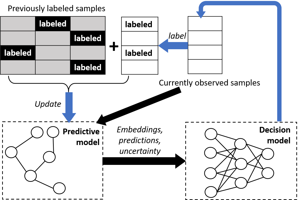
Figure 2: The overview of GR-REAL framework. The black arrows shows the feed-forward process using the predictive model. The blue arrows shows the feedback process by the decision model.

4.1 Recurrent Graph Neural Network

Effective modeling of river segments requires the ability to capture their temporal thermodynamics and the influence received from upstream segments. Hence, we incorporate the information from both previous time steps and neighbors (i.e., upstream segments) when modeling each segment. Our model is based on the LSTM model which has proven to be effective in capturing long-term dependencies. Different from the standard LSTM, we develop a customized recurrent cell that combines the spatial and temporal context.

When applied to each segment $i$ at time $t$, the recurrent cell has a cell state $\textbf{c}_{i}^{t}\in\mathbb{R}^{H}$, which serves as a memory and allows preserving the information from its history and neighborhood. Then the recurrent cell outputs a hidden representation $\textbf{h}_{i}^{t}\in\mathbb{R}^{H}$, from which we generate the target output. In the following, we describe the recurrent process of generating $\textbf{c}_{i}^{t}$ and $\textbf{h}_{i}^{t}$ based on the input $\textbf{x}_{i}^{t}$ and collected information from the previous time $t-1$.

For each river segment $i$ at time $t-1$, the model extracts latent variables which contain relevant information to pass to its downriver segments. We refer to these latent variables as transferred variables. For example, the amount of water advected from each segment and its water temperature can directly impact the change of water temperature for its downriver segments. We generate the transferred variables $\textbf{q}_{i}^{t-1}$ from the hidden representation $\textbf{h}_{i}^{t-1}$ at the previous time step:

(4.1) $$\small\textbf{q}_{i}^{t-1}=\text{tanh}(\textbf{U}_{q}\textbf{h}_{i}^{t-1}+\textbf{b}_{q}),$$

where $\textbf{U}_{q}$ and $\textbf{b}_{q}$ are model parameters.

Similar to LSTM, we generate a candidate cell state $\bar{\textbf{c}}_{i}^{t}$, a forget gate $f_{i}^{t}$ and a input gate $g_{i}^{t}$ by combining $\textbf{{x}}_{i}^{t}$ and the hidden representation at previous time step $\textbf{h}_{i}^{t-1}$, as follows:

(4.2) $$\bar{\textbf{c}}_{i}^{t} =\text{tanh}(\textbf{U}_{c}\textbf{h}_{i}^{t-1}+\textbf{V}_{c}\textbf{x}_{i}^{t}+\textbf{b}_{c}),$$

$$\textbf{f}_{i}^{t} =\sigma(\textbf{U}_{f}\textbf{h}_{i}^{t-1}+\textbf{V}_{f}\textbf{x}_{i}^{t}+\textbf{b}_{f}),$$

$$\textbf{g}_{i}^{t} =\sigma(\textbf{U}_{g}\textbf{h}_{i}^{t-1}+\textbf{V}_{g}\textbf{x}_{i}^{t}+\textbf{b}_{g}),$$

where $\{\textbf{U}_{l},\textbf{V}_{l},\textbf{b}_{l}\}_{l=c,f,g}$ are model parameters.

After gathering the transferred variables for all the segments, we develop a new recurrent cell structure for each segment $i$ that integrates the transferred variables from its upstream segments into the computation of the cell state $\textbf{c}_{i}^{t}$. The forget gate $\textbf{f}_{i}^{t}$ and input gate $\textbf{g}_{i}^{t}$ are used to filter the information from previous time step and current time. This process can be expressed as:

(4.3) $$\small\textbf{c}_{i}^{t}=\textbf{f}_{i}^{t}\otimes(\textbf{c}_{i}^{t-1}+\sum_{(j,i)\in\mathcal{E}}\textbf{W}_{ji}\textbf{q}_{j}^{t-1})+\textbf{g}_{i}^{t}\otimes\bar{\textbf{c}}_{i}^{t},$$

where $\otimes$ denotes the entry-wise product.

We can observe that the forget gate not only filters the previous information from the segment $i$ itself but also from its neighbors (i.e., upstream segments). Each upstream segment $j$ is weighted by the adjacency level $\textbf{A}_{ji}$ between $j$ and $i$. When a river segment has no upstream segments (i.e., head water), the computation of $\textbf{c}_{i}^{t}$ is the same as with the standard LSTM. In Eq. 4.3, we use $\textbf{q}_{j}^{t-1}$ from the previous time step because of the time delay in transferring the influence from upstream to downriver segments (the maximum travel time is approximately one day according to PRMS).

Then we generate the output gate $\textbf{o}^{t}_{i}$ to filter the cell state at $t$ and output the hidden representation:

(4.4) $$\textbf{o}_{i}^{t} =\sigma(\textbf{U}_{o}\textbf{h}_{i}^{t-1}+\textbf{V}_{o}\textbf{x}_{i}^{t}+\textbf{b}_{o}),$$

$$\textbf{h}_{i}^{t} =\textbf{o}_{i}^{t}\otimes\text{tanh}(\textbf{c}_{i}^{t}),$$

where $\{\textbf{U}_{o},\textbf{V}_{o},\textbf{b}_{o}\}$ are model parameters.

Finally, we generate the predicted output from the hidden representation as follows:

(4.5) $$\small\hat{\textbf{y}}_{i}^{t}=\textbf{W}_{y}\textbf{h}_{i}^{t}+\textbf{b}_{y},$$

where $\textbf{W}_{y}$ and $\textbf{b}_{y}$ are model parameters.

After applying this recurrent process to all the time steps, we define a loss using true observations $\textbf{Y}=\{\textbf{y}_{i}^{t}\}$ that are collected at certain time steps and certain segments, as follows:

(4.6) $$\small\mathcal{L}_{\text{RGrN}}=\frac{1}{|\textbf{Y}|}\sum_{\{(i,t)|\textbf{y}_{i}^{t}\in\textbf{Y}\}}(\textbf{y}_{i}^{t}-\hat{\textbf{y}}_{i}^{t})^{2}.$$

4.2 Markov Decision Process for Active Learning

The real-time labeling problem can be naturally formulated as a Markov sequential decision making problem. Here each state corresponds to the current status of the predictive model given the input of currently observed samples. Given the current state, an intelligent agent (i.e., the decision model) needs to take the optimal actions that maximize the potential reward. Here the actions represent the decisions of whether we will label each river segment at the current time $t$. The reward can be measured by the improvement of predictive performance on an independent hold-out dataset. Our goal is to get a decision model that can maximize the gain of performance improvement.

Specifically, we represent the state variable at each time $t$ as $\textbf{S}^{t}\in\mathbb{R}^{N\times(H+3)}$, where each row $\textbf{s}_{i}^{t}=[\textbf{h}_{i}^{t},\hat{\textbf{y}}_{i}^{t},\textbf{u}_{i}^{t},\textbf{b}^{t}]$ is the concatenation of model embeddings $\textbf{h}_{i}^{t}$, prediction $\hat{\textbf{y}}_{i}^{t}$, and uncertainty $\textbf{u}_{i}^{t}$ of the segment $i$ obtained from the predictive model, as well as the remaining budget $\textbf{b}^{t}$. Here the uncertainty level is estimated by Monte Carlo drop-out-based strategy used in previous work [5, 9]. Actions taken at each time are encoded by an $N$-by-$2$ matrix $\textbf{A}^{t}$ where each row $\textbf{a}^{t}_{i.}$ is a one-hot vector indicating whether we label the segment $i$ ([1, 0]) or not ([0, 1]).

The decision model is used to determine optimal actions to take at each time. In particular, the decision model takes the input of current state $\textbf{S}^{t}$ and outputs the potential future reward when the agent performs each possible action $\textbf{A}^{t}$ , i.e., the $Q$ value $Q(\textbf{S}^{t},\textbf{A}^{t})$. To train such a decision model, we need to estimate training labels for the $Q$ values by dynamic programming. Specifically, we consider a set of four-tuple samples over the sequence which consists of $\{\textbf{S}^{t},\textbf{A}^{t},R(\textbf{S}^{t},\textbf{A}^{t}),\textbf{S}^{t+1}\}$, where $R(\textbf{S}^{t},\textbf{A}^{t})$ is the immediate reward of performing actions $\textbf{A}^{t}$ at state $\textbf{S}^{t}$ and this can be measured as the reduction of prediction RMSE on an independent hold-out dataset, and $\textbf{S}^{t+1}$ is the new model state after we observe data at $t+1$. We can estimate the training labels $Q(\textbf{S}^{t},\textbf{A}^{t})$ via dynamic programming, as follows:

(4.7) $$Q(\textbf{S}^{t},\textbf{A}^{t})=R(\textbf{S}^{t},\textbf{A}^{t})+\gamma\max_{\textbf{A}^{t+1}}Q(\textbf{S}^{t+1},\textbf{A}^{t+1}),$$

where $\gamma$ is a discount factor.

During the prediction phase, we can select optimal actions that maximize the $Q$ value, as follows:

(4.8) $$\textbf{A}^{t}_{*}=\text{argmax}_{\textbf{A}^{t}}Q(\textbf{S}^{t},\textbf{A}^{t})$$

Given a large number of river segments, the action space will be exponentially large ($2^{N}$) and thus the model learning can be computationally intractable. In this work, we consider a simplified action space by performing actions independently on each river segment given its current state so we reduce the possible actions to be $2N$. Nevertheless, the selected actions for different river segments are still related to each other since we embed the spatial context of each segment in its state vector.

Algorithm 1 Training procedure of GR-REAL.

0:  Training data $\textbf{X}_{tr}=\{\textbf{x}_{i}^{t}\}$ for $i=1:N$ and $t=1:T1$, and their available labels $\{\textbf{y}_{i}^{t}\}$; Holdout data $\textbf{X}_{hd}=\{\textbf{x}_{i}^{t}\}$ for $i=1:N$ and $t=T1+1:T$, and their available labels $\{\textbf{y}_{i}^{t}\}$;

1:  for training epoch $k\leftarrow 1$ to Train_iteration do

2:     Labeled set $\mathcal{L}=\{\}$, state transition set $\mathcal{M}$={}.

3:     initialize the predictive model.

4:     for time step $t\leftarrow 1$ to $T1$ do

5:        if remaining budget$\leq$0 then

6:           Break

7:        end if

8:        Generate $\textbf{h}^{t}$, $\hat{\textbf{y}}^{t}$, $\textbf{u}^{t}$ by the predictive model.

9:        Concatenate the obtained values into the state vector $\textbf{s}^{t}$.

10:        if $t>1$ then

11:           Add $(\textbf{S}^{t-1},\textbf{S}^{t},\textbf{A}^{t-1},R(\textbf{S}^{t-1},\textbf{A}^{t-1}))$ to $\mathcal{M}$.

12:           Update the decision model using samples in $\mathcal{M}$.

13:        end if

14:        for river segment $i\leftarrow 1$ to $N$ do

15:           Predict $Q(\textbf{s}_{i}^{t},\cdot)$ for different actions by the decision model.

16:           Select the action $\textbf{a}_{i}^{t}$ that leads to the highest $Q$ value.

17:        end for

18:        Update $\mathcal{L}$ with labeled samples and reduce the budget.

19:        Update the predictive model using samples in $\mathcal{L}$ and measure the performance improvement on $\textbf{X}_{hd}$ as the reward $R(\textbf{S}^{t},\textbf{A}^{t})$.

20:     end for

21:  end for

4.3 Implementation details

We summarize the training process in Algorithm 1. Here we wish to clarify the difference between the training procedure and the test procedure. It is noteworthy that we repeatedly train our model by going through the training period for multiple passes (Line 1 in Algorithm 1). This is critical for refining the decision model given the fact that it can make poor decisions (especially for the first few time steps) during the first few passes. When we apply the trained model to the test period (i.e., $T+1$ to $T+M$), we can only take one pass over the test data in a typical setting of real-time active learning. In this case, the decision model cannot change any decisions that have been made in the past.

During the training process, we also allow the selection of random query samples from the training period with a probability of 0.5%. This helps the decision model to explore a diverse set of training samples and thus have a better estimate of the potential reward resulted from each labeling action.

4.4 Policy Transfer

Due to the substantial human effort and material costs to collect observation data, we often have limited data for training ML models. For example, the Delaware River Basin is one of the most widely studied basins in the United States but still has less than 2% daily temperature observation for over 80% of its internal river segments [18]. Such sparse data makes it challenging to train a good decision model.

To address this issue, we propose to transfer the model learned from simulation data produced by physics-based models. Physics-based models are built based on known physical relationships that transform input features to the target variable. In the context of modeling river networks, we use PRMS-SNTemp model to simulate target variables (i.e., temperature and streamflow) given the input drivers. Hence, for the input features $\textbf{x}_{i:N}^{1:T}$ for all the $N$ river segments in a past period with $T$, we can generate their simulated target variables $\textbf{y}_{i:N}^{1:T}$ by running the PRMS-SNTemp model. We can pre-train the decision model using the simulation data. Then we can refine the decision model when it is applied to true observations.

It is noteworthy that simulation data from the PRMS-SNTemp model are imperfect but they only provide a synthetic realization of physical responses of a river systems to a given set of input features. Nevertheless, pre-training a neural network using simulation data allows the network to emulate a synthetic but physically realistic phenomena. When applying the pre-trained model to a real system, we fine-tune the model using true observations. Our hypothesis is that the pre-trained model is much closer to the optimal solution and thus requires less true labeled data to train a good quality model.

5 Experimental Results

5.1 Dataset and test settings

The dataset is pulled from U.S. Geological Survey’s National Water Information System [27] and the Water Quality Portal [18], the largest standardized water quality data set for inland and coastal waterbodies [18]. Observations at a specific latitude and longitude were matched to river segments that vary in length from 48 to 23,120 meters. The river segments were defined by the national geospatial fabric used for the National Hydrologic Model as described by Regan et al. [20], and the river segments are split up to have roughly a one day water travel time. We match observations to river segments by snapping observations to the nearest river segment within a tolerance of 250 meters. Observations farther than 5,000 m along the river channel to the outlet of a segment were omitted from our dataset.

We study a subset of the Delaware River Basin with 42 river segments that feed into the mainstream Delaware River at Wilmington, DE. We use input features at the daily scale from Oct 01, 1980 to Sep 30, 2016 (13,149 dates). The input features have 10 dimensions which include daily average precipitation, daily average air temperature, date of the year, solar radiation, shade fraction, potential evapotranspiration and the geometric features of each segment (e.g., elevation, length, slope and width). Water temperature observations were available for 32 segments but the temperature was observed only on certain dates. The number of temperature observations available for each observed segment ranges from 1 to 9,810 with a total of 51,103 observations across all dates and segments. Streamflow observations were available for 18 segments. The number of streamflow observations available for each observed segment ranges from 4,877 to 13,149 with a total of 206,920 observations across all dates and segments.

We divide the available data into four periods, training period (Oct 01, 1980 - Sep 30, 1989), hold-out period (Oct 01, 1989 - Sep 30, 1998), test period (Oct 01, 1998 - Sep 30, 2007) and evaluation period (Oct 01, 2007 - Sep 30, 2016). We assume the current time $T+1$ starts from Oct 01, 1998, i.e., the start of the testing period. We will apply the trained decision model to the test period to collect new samples and use them to train the predictive model. Then the predictive model will be evaluated in the evaluation period.

We will compare with a set of baselines:

• Random selection: This method assumes the access to the entire set of testing data (so it is a pool-based method). We randomly select a subset of query samples (size equal to the budget) from the test data for labeling.

• Uncertainty: For each time step, we estimate the uncertainty of each data sample (i.e., each node in the graph) using the method presented in previous work [5, 9]. Then we select the query samples if their uncertainty values are above a threshold. Such threshold is estimated in the training period.

• Uncentainty+Centrality+Density (UDC): This is a graph-based active learning method. For each time step, we compute the weighted summation of uncertainty (measured by [5, 9]), the centrality and the density of each node following the previous work [1, 10]. Then we select the query samples if their summation values are above a threshold. Such threshold is estimated in the training period.

• ROAL [11]: This methods solves the real-time labeling problem using reinforcement learning. It considers each segment separately but uses an LSTM to estimate the Q value.

Here the first three baselines use the same predictive model as our proposed GR-REAL method, which uses a one-layer graph structure. Since the adjacency matrix W includes $(i,j)$ pairs for segment $j$ anywhere downstream of segment $i$, the one-layer graph structure can still capture spatial dependencies between river segments that are not directly connected. We generate the adjacency matrix W based on the stream distance between each pair of river segment outlets, represented as $\text{dist}(i,j)$. We standardize the stream distance and then compute the adjacency level as $\textbf{W}_{ij}=1/(1+\text{exp}(\text{dist}(i,j)))$ for each edge $(i,j)\in\mathcal{E}$. The hidden variables in the networks have a dimension of 20. The hyper-parameter $\gamma$ is set as 0.8. For uncertainty estimation, we have used a dropout probability of 0.2 and randomly created 10 different dropout networks. During the training and testing, we also set a yearly limit so as to avoid having too many query samples selected from a single year. Here we set the yearly limit to be $1.2\times\text{Budget}/\#\text{years}$

5.2 Predictive performance

Table 1: RMSE (standard deviation) for streamflow modeling ($m^{3}/s$) with different budgets.

Samples	100	300	500	1000	2000
Random	6.24	5.97	5.92	5.66	5.59
	(0.52)	(0.34)	(0.36)	(0.20)	(0.23)
Uncertain	6.16	5.88	5.83	5.64	5.43
	(0.26)	(0.24)	(0.20)	(0.12)	(0.14)
UDC	6.12	5.84	5.76	5.49	5.44
	(0.23)	(0.26)	(0.19)	(0.12)	(0.12)
ROAL	5.79	5.74	5.70	5.22	5.36
	(0.25)	(0.22)	(0.13)	(0.11)	(0.11)
GR-REAL	5.33	5.40	5.41	4.80	4.78
	(0.21)	(0.22)	(0.14)	(0.11)	(0.08)

Table 2: RMSE (standard deviation) for temperature modeling (${}^{\circ}C$) with different budgets.

Samples	100	300	500	1000	2000
Random	4.42	3.89	3.42	3.31	3.25
	(0.45)	(0.46)	(0.34)	(0.14)	(0.09)
Uncertain	4.16	3.51	3.40	3.28	3.27
	(0.38)	(0.35)	(0.35)	(0.17)	(0.06)
UDC	4.17	3.56	3.33	3.24	3.26
	(0.29)	(0.24)	(0.26)	(0.12)	(0.04)
ROAL	4.04	3.54	3.38	3.24	3.24
	(0.27)	(0.19)	(0.19)	(0.13)	(0.08)
GR-REAL	3.40	3.34	3.29	3.23	3.24
	(0.18)	(0.16)	(0.15)	(0.09)	(0.05)

In Tables 1 and 2, we report the performance of each method with different budget limits (i.e., the number of allowed labeled samples). We repeat each method five times and report mean and standard deviation of prediction RMSE (in the evaluation period). In general, the proposed GR-REAL outperforms other methods by a considerable margin. For temperature modeling, all the methods have similar performance when they have access to sufficient labeled samples (e.g., 2000 samples), but GR-REAL outperforms other methods when we have limited budget. Here the method based on model uncertainty, node density and centrality can be less helpful because these measures indicate only the representativeness of samples at the current time but not the potential future benefit in a real-time sequence. The ROAL method also does not perform as well as the proposed method as it does not take into account the spatial context when estimating the potential reward of labeling each sample.

Figure 3: The relationship between the number of selected query samples and the change of prediction RMSE over time.

In Fig. 3, we show an example for the selected samples by GR-REAL in streamflow modeling (training period). It can be clearly seen that the many samples are labeled right at the time when the predictive model starts to get an increase of prediction error. Then the error decreases after we refine the model using the labeled samples. This shows the effectiveness of the proposed method in automatically detecting query samples which can bring large potential benefit for model training.

5.3 Distribution of selected data

In Fig. 4, we show the distribution of selected data samples over the entire test period for temperature prediction. Given the budget limit of 1000, we observe that GR-REAL selects most samples in the summer period (Fig. 4 (a)), especially before 2004. This is because river temperature in the Delaware River Basin are usually much more variable in summer period and thus more samples are selected to learn these complex dynamic patterns. Since 2004, the model selects fewer data on the same “peak” period since the potential reward for training the model decreases after it has learned from samples in the same period from previous years. When we reduce the budget to 500, GR-REAL also selects more samples in other time periods than the summer period (especially after 2004) because the budget is limited and the model needs to balance the performance over the entire year to get the optimal overall performance.

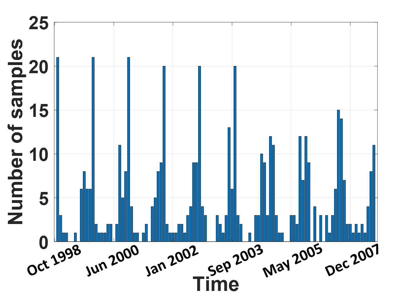
Figure 4: The distribution of selected query sample over time for temperature modeling given the budget of (a) 1000 and (b) 500.

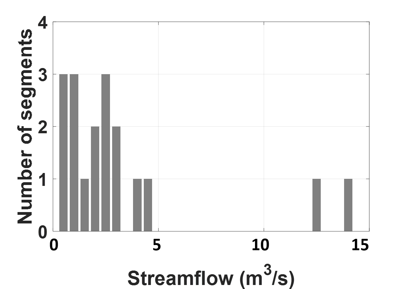
Figure 5: (a) Number of river segments for each streamflow range. (b) Distribution of selected samples over river segments of different streamflow ranges.

For the streamflow modeling, we show the distribution of selected samples over segments with different streamflow ranges. For each segment, we first compute its average streamflow value and we show the histogram of average streamflow over all the 18 segments (which have streamflow observations) in Fig. 5 (a). Then we show in Fig. 5 (b) the distribution of selected samples with respect to the average streamflow of the segments from which the samples are taken. We can see that most samples are selected from the two segments with largest streamflow values and from the segments with average streamflow around 3$m^{3}/s$. We hypothesize that labeled samples from segments with highstreamflow ($>12m^{3}/s$) and middle flow range($1-5m^{3}/s$) are more helpful to refine the model so as to reduce the overall prediction error. In contrast, more samples on low-flow range ($<1m^{3}/s$) can bring limited improvement to the overall error because errors made on low-flow segments tend to be much smaller. This is one limitation of the proposed method as accurate prediction on low-flow segments is also important for understanding the aquatic ecosystem. These limitations may be potential opportunities for future work.

5.4 Performance of different graph models

Here we show how the representation of graphs impacts the learning performance (Table. 3). We consider the following three representation: 1) Downstream-neighbor graph which is the graph used in our implementation. Here we add edges from segment $i$ to segment $j$ if segment $j$ is anywhere downstream of segment $i$. Consider three segments $\{a,b,c\}$ in a upstream-to-downstream consecutive sequence. We will include the edge $ab$, $bc$ and $ac$ in our graph and their adjacency levels are determined by the stream distance. 2) Direct-neighbor graph which only includes connected neighbors. In the above example, we will only create edges of $ab$ and $bc$. 3) No-neighbor graph which is equivalent to an RNN model trained using data from all the segments. The choice of graph representation can affect the selection of representative samples. The improvement from no-neighbor graph to direct-neighbor graph shows that the modeling of spatial context can help select more informative samples. The downstream-neighbor graph results in better performance since a river segment can impact downriver segments that are multi-hops away and thus incorporating multi-hop relationships can help better embed the contextual information.

Table 3: The prediction RMSE (budget=500) using different graph structures.

Graph	streamflow($m^{3}/s$)	temperature(${}^{\circ}C$)
Downstream neighbor	5.41	3.29
Direct neighbor	5.57	3.33
No neighbor	5.71	3.36

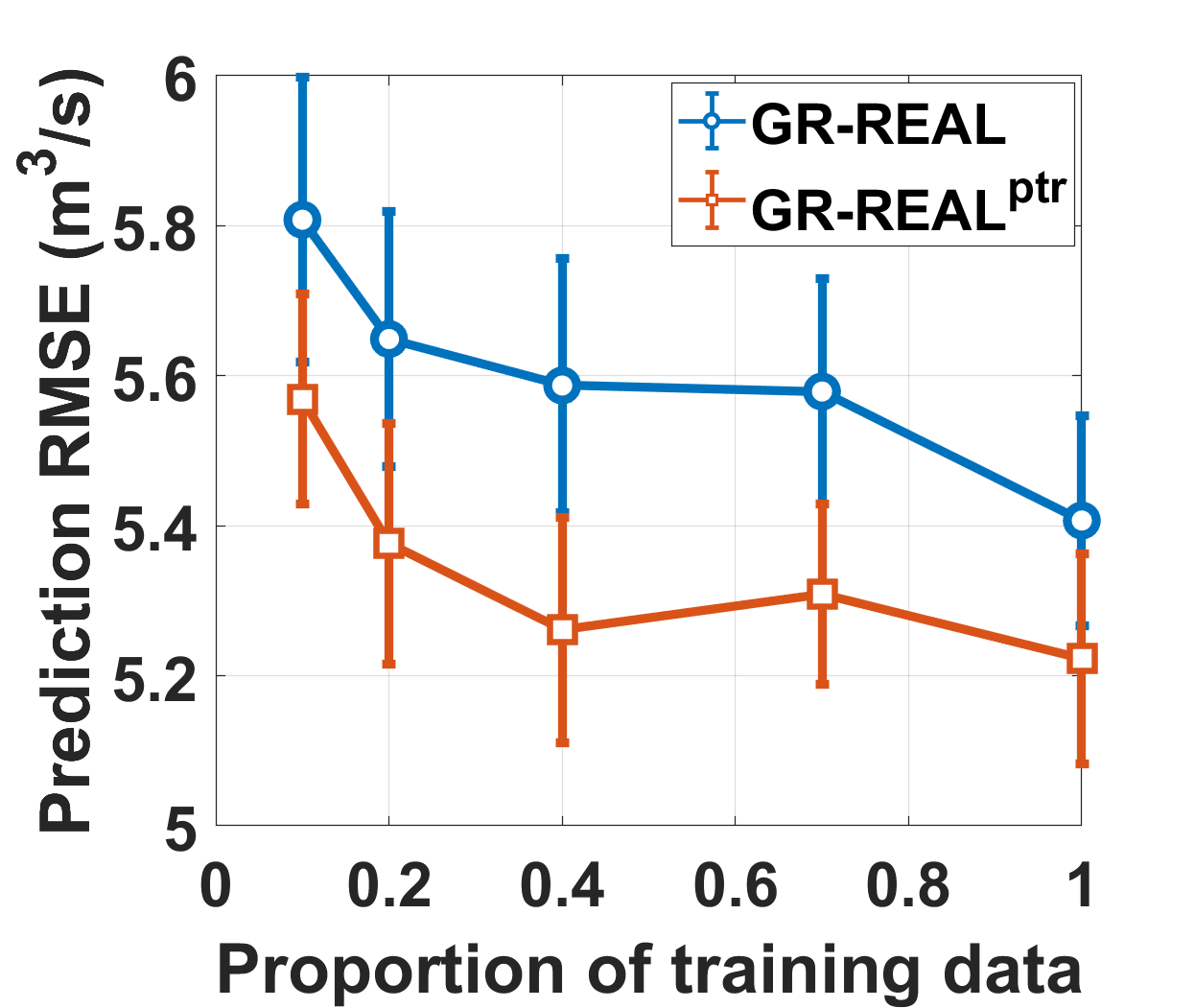
Figure 6: Prediction performance of GR-REAL before and after using the policy transfer in modeling (a) streamflow and (b) water temperature.

5.5 Policy transfer

We also study the efficacy of policy transfer from simulation data when we have access to limited training data. In particular, we randomly reduce the labeled samples for temperature and streamflow in the training period so that GR-REAL will learn different decision models. Then we will evaluate the performance using these decision models as reported in Fig. 6. We can observe that the predictive performance decreases as we reduce the number of training data. This is because we can only learn a sub-optimal decision model using limited training data and thus it may not be able to select the most helpful samples for training the predictive model. However, the method with policy transfer (GR-REAL${}^{\text{ptr}}$) can produce better performance since the model is initialized to be much closer to its optimal state. In temperature prediction, we notice that GR-REAL and GR-REAL${}^{\text{ptr}}$ have similar performance when using more than 70% training data. This is because the training data is sufficient to learn an accurate decision model.

6 Conclusion

In this paper, we propose the GR-REAL framework which uses the spatial and temporal contextual information to select query samples in real time. We demonstrate the effectiveness of GR-REAL in selecting informative samples for modeling streamflow and water temperature in the Delaware River Basin. We also show that policy transfer can further improve the performance when we have less training data. The proposed method may also be used to measure other water quality parameters for which sensors are costly or too difficult to maintain (e.g., metal, nutrients, or algal biomass).

While GR-REAL achieves better predictive performance, it estimates potential reward based on accuracy improvement and thus remains limited in selecting samples that indeed help understand an ecosystem. For example, the GR-REAL ignores low-flow segments as they contribute less to the overall accuracy loss. Studying this element of GR-REAL has promise for future work.

7 Acknowledgments

Any use of trade, firm, or product names is for descriptive purposes only and does not imply endorsement by the U.S. Government.

References

- [1] Hongyun Cai et al. Active learning for graph embedding. arXiv preprint arXiv:1705.05085, 2017.
- [2] Yu Cheng et al. Feedback-driven multiclass active learning for data streams. In CIKM, 2013.
- [3] David A Cohn et al. Active learning with statistical models. JAIR, 1996.
- [4] Ido Dagan and Sean P Engelson. Committee-based sampling for training probabilistic classifiers. In Machine Learning Proceedings. Elsevier, 1995.
- [5] Arka Daw et al. Physics-guided architecture (pga) of neural networks for quantifying uncertainty in lake temperature modeling. In SDM. SIAM, 2020.
- [6] James H Faghmous and Vipin Kumar. A big data guide to understanding climate change: The case for theory-guided data science. Big data, 2014.
- [7] Richard M Felder and Rebecca Brent. Active learning: An introduction. ASQ higher education brief, 2(4):1–5, 2009.
- [8] Yarin Gal et al. Deep bayesian active learning with image data. arXiv preprint arXiv:1703.02910, 2017.
- [9] Yarin Gal and Zoubin Ghahramani. Dropout as a bayesian approximation: Representing model uncertainty in deep learning. In ICML, 2016.
- [10] Li Gao et al. Active discriminative network representation learning. In IJCAI, 2018.
- [11] Honglan Huang et al. On the improvement of reinforcement active learning with the involvement of cross entropy to address one-shot learning problem. PloS one, 2019.
- [12] Xiaowei Jia et al. Physics guided rnns for modeling dynamical systems: A case study in simulating lake temperature profiles. In SDM, 2019.
- [13] Alex Kendall and Yarin Gal. What uncertainties do we need in bayesian deep learning for computer vision? In NeurIPS, 2017.
- [14] Jacob H LaFontaine, Lauren E Hay, Roland J Viger, Steve L Markstrom, R Steve Regan, Caroline M Elliott, and John W Jones. Application of the precipitation-runoff modeling system (prms) in the apalachicola-chattahoochee-flint river basin in the southeastern united states. US Geological Survey Scientific Investigations Report, 5162:1–118, 2013.
- [15] Xin Li and Yuhong Guo. Adaptive active learning for image classification. In CVPR, 2013.
- [16] Steven L Markstrom, Robert S Regan, Lauren E Hay, Roland J Viger, Richard MT Webb, Robert A Payn, and Jacob H LaFontaine. Prms-iv, the precipitation-runoff modeling system, version 4. U.S. Geological Survey Techniques and Methods, book 6, chap B7, 2015.
- [17] Yanlin Qi et al. A hybrid model for spatiotemporal forecasting of pm2. 5 based on graph convolutional neural network and long short-term memory. Science of the Total Environment, 2019.
- [18] Emily K Read et al. Water quality data for national-scale aquatic research: The water quality portal. Water Resources Research, 2017.
- [19] Jordan S Read et al. Process-guided deep learning predictions of lake water temperature. WRR, 2019.
- [20] R Steven Regan, Steven L Markstrom, Lauren E Hay, Roland J Viger, Parker A Norton, Jessica M Driscoll, and Jacob H LaFontaine. Description of the national hydrologic model for use with the precipitation-runoff modeling system (prms). Technical report, US Geological Survey, 2018.
- [21] Michael J Sanders, Steven L Markstrom, R Steven Regan, and R Dwight Atkinson. Documentation of a daily mean stream temperature module—an enhancement to the precipitation-runoff modeling system. Technical report, U.S. Geological Survey Techniques and Methods, book 6, chap. D4, 2017.
- [22] Ozan Sener and Silvio Savarese. Active learning for convolutional neural networks: A core-set approach. arXiv preprint arXiv:1708.00489, 2017.
- [23] Burr Settles. Active learning literature survey. Technical report, University of Wisconsin-Madison Department of Computer Sciences, 2009.
- [24] Shital Shah et al. Airsim: High-fidelity visual and physical simulation for autonomous vehicles. In Field and service robotics. Springer, 2018.
- [25] Yanyao Shen et al. Deep active learning for named entity recognition. arXiv preprint:1707.05928, 2017.
- [26] Jasmina Smailović et al. Stream-based active learning for sentiment analysis in the financial domain. Information sciences, 2014.
- [27] U.S. Geological Survey. Usgs water data for the nation: U.s. geological survey national water information system database. https://doi.org/10.5066/f7p55kjn, 2016. Accessed: June 2019.
- [28] Sarah Wassermann, Thibaut Cuvelier, and Pedro Casas. Ral-improving stream-based active learning by reinforcement learning. 2019.
- [29] Yuexin Wu et al. Active learning for graph neural networks via node feature propagation. arXiv preprint arXiv:1910.07567, 2019.
- [30] Tian Xie et al. Crystal graph convolutional neural networks for an accurate and interpretable prediction of material properties. Physical review letters, 2018.
- [31] Alireza Yazdani et al. Systems biology informed deep learning for inferring parameters and hidden dynamics. bioRxiv, 2019.
- [32] Shusen Zhou et al. Active deep learning method for semi-supervised sentiment classification. Neurocomputing, 2013.