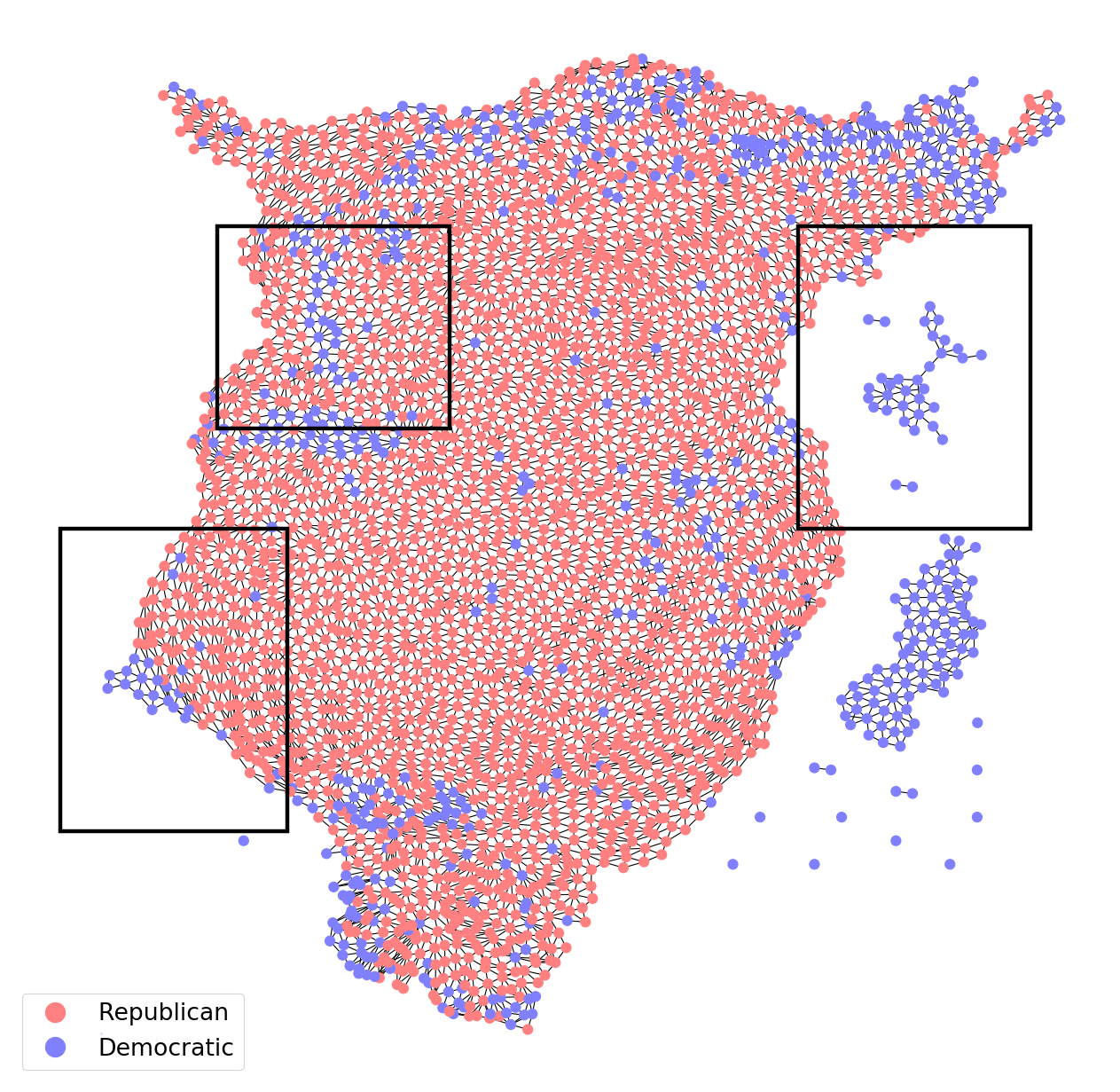
Combining Label Propagation and Simple Models out-performs Graph Neural Networks
Abstract
Graph Neural Networks (GNNs) are the predominant technique for learning over graphs. However, there is relatively little understanding of why GNNs are successful in practice and whether they are necessary for good performance. Here, we show that for many standard transductive node classification benchmarks, we can exceed or match the performance of state-of-the-art GNNs by combining shallow models that ignore the graph structure with two simple post-processing steps that exploit correlation in the label structure: (i) an “error correlation” that spreads residual errors in training data to correct errors in test data and (ii) a “prediction correlation” that smooths the predictions on the test data. We call this overall procedure Correct and Smooth (C&S), and the post-processing steps are implemented via simple modifications to standard label propagation techniques from early graph-based semi-supervised learning methods. Our approach exceeds or nearly matches the performance of state-of-the-art GNNs on a wide variety of benchmarks, with just a small fraction of the parameters and orders of magnitude faster runtime. For instance, we exceed the best known GNN performance on the OGB-Products dataset with 137 times fewer parameters and greater than 100 times less training time. The performance of our methods highlights how directly incorporating label information into the learning algorithm (as was done in traditional techniques) yields easy and substantial performance gains. We can also incorporate our techniques into big GNN models, providing modest gains. Our code for the OGB results is at https://github.com/CUAI/CorrectAndSmooth.
1 Introduction
Following the success of neural networks in computer vision and natural language processing, there are now a wide range of graph neural networks (GNNs) for making predictions involving relational data (Battaglia et al., 2018; Wu et al., 2020). These models have had much success and sit atop leaderboards such as the Open Graph Benchmark (Hu et al., 2020). Often, the methodological developments for GNNs revolve around creating strictly more expressive architectures than basic variants such as the Graph Convolutional Network (GCN) (Kipf & Welling, 2017) or GraphSAGE (Hamilton et al., 2017a); examples include Graph Attention Networks (Veličković et al., 2018), Graph Isomorphism Networks (Xu et al., 2018), and various deep models (Li et al., 2019; Rong et al., 2019; Chen et al., 2020). Many ideas for new GNN architectures are adapted from new architectures in models for language (e.g., attention) or vision (e.g., deep CNNs) with the hopes that success will translate to graphs. However, as these models become more complex, understanding their performance gains is a major challenge, and scaling them to large datasets is difficult.
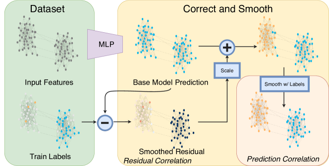
Here, we see how far we can get by combining much simpler models, with an emphasis on understanding where there are easy opportunities for performance improvements in graph learning, particularly transductive node classification. We propose a simple pipeline with three main parts (Figure 1): (i) a base prediction made with node features that ignores the graph structure (e.g., an MLP or linear model); (ii) a correction step, which propagates uncertainties from the training data across the graph to correct the base prediction; and (iii) a smoothing of the predictions over the graph. Steps (ii) and (iii) are just post-processing and use classical methods for graph-based semi-supervised learning, namely, label propagation (Zhu, 2005).111One of the main methods that we use (Zhou et al., 2004) is often called label spreading. The term “label propagation” is used in a variety of contexts (Zhu, 2005; Wang & Zhang, 2007; Raghavan et al., 2007; Gleich & Mahoney, 2015). The salient point for this paper is that we assume positive correlations on neighboring nodes and that the algorithms work by “propagating” information from one node to another. With a few modifications and new deployment of these classic ideas, we achieve state-of-the-art performance on several node classification tasks, outperforming big GNN models. In our framework, the graph structure is not used to learn parameters but instead as a post-processing mechanism. This simplicity leads to models with orders of magnitude fewer parameters that take orders of magnitude less time to train and can easily scale to large graphs. We can also combine our ideas with state-of-the-art GNNs and see modest performance gains.
A major source of our performance improvements is directly using labels for predictions. This idea is not new — early diffusion-based semi-supervised learning algorithms on graphs such as the spectral graph transducer (Joachims, 2003), Gaussian random field models (Zhu et al., 2003), and and label spreading (Zhou et al., 2004) all use this idea. However, the motivation for these methods was semi-supervised learning on point cloud data, so the features were used to construct the graph. Since then, these techniques have been used for learning on relational data from just the labels (i.e., no features) (Koutra et al., 2011; Gleich & Mahoney, 2015; Peel, 2017; Chin et al., 2019) but have largely been ignored in GNNs. That being said, we find that even simple label propagation (which ignores features) does surprisingly well on a number of benchmarks. This provides motivation for combining two orthogonal sources of prediction power — one coming from the node features (ignoring graph structure) and one coming from using the known labels directly in predictions.
Recent research connects GNNs to label propagation (Wang & Leskovec, 2020; Jia & Benson, 2020) as well as Markov Random fields (Qu et al., 2019; Gao et al., 2019), and some techniques use ad hoc incorporation of label information in the features (Shi et al., 2020). However, these approaches are still expensive to train, while we use label propagation in two understandable and low-cost ways. We start with a cheap “base prediction” from a model that ignores graph structure (apart from perhaps a cheap pre-processing feature augmentation step like a spectral embedding). After, we use label propagation for error correction and then to smooth final predictions. These post-processing steps are based on the fact that errors and labels on connected nodes are positively correlated. Assuming similarity between connected nodes is at the center of much network analysis and corresponds to homophily or assortative mixing (McPherson et al., 2001; Newman, 2003; Easley & Kleinberg, 2010). In the semi-supervised learning literature, the analog is the smoothness or cluster assumption (Chapelle et al., 2003; Zhu, 2005). The good performance of label propagation that we see across a wide variety of datasets suggests that these correlations hold on common benchmarks.
Overall, our methodology demonstrates that combining several simple ideas yields excellent performance in transductive node classification at a fraction of the cost, in terms of both model size (i.e., number of parameters) and training time. For example, on the OGB-Products benchmark, we out-perform the current best-known GNN with more than two orders of magnitude fewer parameters and more than two orders of magnitude less training time. However, our goal is not to say that current graph learning methods are poor or inappropriate. Instead, we aim to highlight easier ways in which to improve prediction performance in graph learning and to better understand the source of performance gains. Our main finding is that more direct incorporation of labels into the learning algorithms is key. And by combining our ideas with existing GNNs, we also see improvements, although they are minor. We hope that our approach spurs new ideas that can help in other graph learning tasks, such as inductive node classification, link prediction, and graph prediction.
1.1 Additional related work
The Approximate Personalized Propagation of Neural Predictions (APPNP) framework is most relevant to our work, as they also smooth base predictions (Klicpera et al., 2018). However, they focus on integrating this smoothing into the training process so that their model can be trained end to end. Not only is this significantly more computationally expensive, it also prevents APPNP from incorporating label information at inference. Compared to APPNP, our framework produces more accurate predictions, is faster to train, and more easily scales to large datasets. Our framework also complements the Simplified Graph Convolution (Wu et al., 2019), as well as algorithms designed to increase scalability (Bojchevski et al., 2020; Zeng et al., 2019; Rossi et al., 2020). The primary focus of our approach, however, is using labels directly, and scalability is a byproduct. There is also prior work connecting GCNs and label propagation. Wang & Leskovec (2020) use label propagation as a pre-processing step to weight edges for GNNs, whereas we use label propagation as a post-processing step and avoid GNNs. Jia & Benson (2020) use label propagation with GNNs for regression tasks, and our error correction step adapts some of their ideas for the case of classification. Finally, there are several recent approaches that incorporate nonlinearity into label propagation methods to compete with GNNs and achieve scalability (Eliav & Cohen, 2018; Ibrahim & Gleich, 2019; Tudisco et al., 2020), but these methods focus on settings of low label rates and don’t incorporate feature learning.
2 Correct and Smooth Model
We start with some notation. We assume that we have an undirected graph , where there are nodes with features on each node represented by a matrix . Let be the adjacency matrix of the graph, be the diagonal degree matrix, and be the normalized adjacency matrix . For the prediction problem, the node set is split into a disjoint set of unlabeled nodes and labeled nodes , which are subsets of the indices . We represent the labels by a one-hot-encoding matrix , where is the number of classes (i.e., if is in class , and 0 otherwise), and we further split the labeled nodes into a training set and validation set . Our problem is transductive node classification: assign each node a label in , given , , and .
Our approach starts with a simple base predictor on node features, which does not rely on any learning over the graph. After, we perform two types of label propagation (LP): one that corrects the base predictions by modeling correlated error and one that smooths the final prediction. We call the combination of these two methods Correct and Smooth (C&S; Figure 1). The LPs are only post-processing steps — our pipeline is not trained end-to-end. Furthermore, the graph is only used in these post-processing steps and in a pre-processing step to augment the features , but not for the base predictions. This makes training fast and scalable compared to standard GNN models. Moreover, we take advantage of both LP (which tends to perform fairly well on its own without features) and the node features. We will see that combining these complementary signals yields excellent predictions.
2.1 Simple base predictor
To start, we use a simple base predictor that does not rely on the graph structure. More specifically, we train a model to minimize , where is the th row of , is the th row of , and is a loss function. For this paper, is either a linear model or a shallow multi-layer perceptron (MLP) followed by a softmax, and is the cross-entropy loss. The validation set is used to tune hyperparameters such as learning rates and the hidden layer dimensions for the MLP. From , we get a base prediction , where each row of is a probability distribution resulting from the softmax. Omitting the graph structure for these base predictions avoids the scalability issues with GNNs. In principle, though, we can use any base predictor for , including those based on GNNs, and we explore this in Section 3. However, for our pipeline to be simple and scalable, we just use linear classifiers or MLPs with subsequent post-processing, which we describe next.
2.2 Correcting for error in base predictions with residual propagation
Next, we improve the accuracy of the base prediction by incorporating labels to correlate errors. The key idea is that we expect errors in the base prediction to be positively correlated along edges in the graph. In other words, an error at node increases the chance of a similar error at neighboring nodes of . We should “spread” such uncertainty over the graph. Our approach here is inspired in part by residual propagation (Jia & Benson, 2020), where a similar concept is used for node regression tasks, as well as generalized least squares and correlated error models more broadly (Shalizi, 2013).
To this end, we first define an error matrix , where error is the residual on the training data and zero elsewhere:
| (1) |
The residuals in rows of corresponding to training nodes are zero only when the base predictor makes a perfect predictions. We smooth the error using the label spreading technique of Zhou et al. (2004), optimizing the objective
| (2) |
The first term encourages smoothness of the error estimation over the graph, and is equal to , where is the th column of . The second term keeps the solution close to the initial guess of the error. As in Zhou et al. (2004), the solution can be obtained via the iteration , where and , which converges rapidly to . This iteration is a diffusion, propagation, or spreading of the error, and we add the smoothed errors to the base prediction to get corrected predictions . We emphasize that this is a post-processing technique and there is no coupled training with the base predictions.
This type of propagation is provably the right approach under a Gaussian assumption in regression problems (Jia & Benson, 2020); however, for the classification problems we consider, the smoothed errors might not be at the right scale. We know that in general,
| (3) |
When , we then have that . Thus, the propagation cannot completely correct the errors on all nodes in the graph, as it does not have enough “total mass,” and we find that adjusting the scale of the residual can help substantially in practice. To do this, we propose two variations of scaling the residual.
Autoscale. Intuitively, we want to scale the size of errors in to be approximately the size of the errors in . We only know the true errors at labeled nodes, so we approximate the scale with the average error over the training nodes. Formally, let correspond to the th row of , and define . Then the corrected predictions on an unlabeled node is given by for .
Scaled Fixed Diffusion (FDiff-scale). Alternatively, we can use a diffusion like the one from Zhu et al. (2003), which keeps the known errors at training nodes fixed. More specifically, we iterate and keep fixed until convergence to , starting with . Intuitively, this fixes error values where we know the error (on the labeled nodes ), while other nodes keep averaging over the values of their neighbors until convergence. With this type of propagation, the maximum and minimum values of entries in do not go beyond those in . We still find it effective to learn a scaling hyperparameter to produce .
2.3 Smoothing final predictions with Prediction Correlation
At this point, we have a score vector , obtained from correcting the base predictor with a model for the correlated error . To make a final prediction, we further smooth the corrected predictions. The motivation is that adjacent nodes in the graph are likely to have similar labels, which is expected given homophily or assortative properties of a network. Thus, we can encourage smoothness over the distribution over labels by another label propagation. First, we start with our best guess of the labels:
| (4) |
Here, we set the training nodes back to their true labels and use the corrected predictions for the validation and unlabeled nodes (we can also use the true validation labels, which we discuss later in the experiments). We then iterate with until convergence to give the final prediction . The classification for a node is .
As with error correlation, the smoothing here is a post-processing step, decoupled from the other steps. This type of prediction smoothing is similar in spirit to APPNP (Klicpera et al., 2018), which we compare against later. However, APPNP is trained end-to-end, propagates on final-layer representations instead of softmaxes, does not use labels, and is motivated differently.
2.4 Summary and additional considerations
To review our pipeline, we start with a cheap base prediction , using only node features but not the graph structure. After, we estimate errors by propagating known errors on the training data, resulting in error-corrected predictions . Finally, we treat these as score vectors on unlabeled nodes, and combine them with the known labels through another LP step to produce smoothed final predictions. We refer to this general pipeline as Correct and Smooth (C&S).
Before showing that this pipeline achieves state-of-the-art performance on transductive node classification, we briefly describe another simple way of improving performance: feature augmentation. The hallmark of deep learning is that we can learn features instead of engineering them. However, GNNs still rely on informative input features to make predictions. There are numerous ways to get useful features from just the graph topology to augment the raw node features (Henderson et al., 2011; 2012; Hamilton et al., 2017b). In our pipeline, we augment features with a regularized spectral embedding (Chaudhuri et al., 2012; Zhang & Rohe, 2018) coming from the leading eigenvectors of the matrix , where is a vector of all ones, is a regularization parameter set to the average degree, and is diagonal with th diagonal entry equal to . The underlying matrix is dense, but we can apply matrix-vector products in time linear in the number of edges and use iterative eigensolvers to compute the embeddings quickly.
3 Experiments on Transductive Node Classification
| Datasets | Classes | Nodes | Edges | Parameter | Accuracy | Time |
|---|---|---|---|---|---|---|
| Arxiv | 40 | 169,343 | 1,166,243 | -84.9% | + 0.97 | 9.89 s |
| Products | 47 | 2,449,029 | 61,859,140 | -93.47% | +1.53 | 170.6 s |
| Cora | 7 | 2,708 | 5,429 | -98.37% | + 1.09 | 0.5 s |
| Citeseer | 6 | 3,327 | 4,732 | -89.68% | - 0.69 | 0.48 s |
| Pubmed | 3 | 19,717 | 44,338 | -96.00% | - 0.30 | 0.85 s |
| 42 | 1,005 | 25,571 | - 97.89% | + 4.26 | 42.83 s | |
| Rice31 | 10 | 4,087 | 184,828 | - 99.02% | + 1.39 | 39.33 s |
| US County | 2 | 3,234 | 12,717 | - 74.56% | + 1.77 | 39.05 s |
| wikiCS | 10 | 11,701 | 216,123 | - 84.88% | + 2.03 | 7.09 s |
To demonstrate the effectiveness of our methods, we use nine datasets (Table 1). The Arxiv and Products datasets are from the Open Graph Benchmark (OGB) (Hu et al., 2020); the Cora, Citeseer, and Pubmed are three classic citation network benchmarks (Getoor et al., 2001; Getoor, 2005; Namata et al., 2012); and wikiCS is a web graph (Mernyei & Cangea, 2020). In these datasets, classes are categories of papers, products, or pages, and features are derived from text. We also use a Facebook social network of Rice University, where classes are dorm residences and features are attributes such as gender, major, and class year, amongst others (Traud et al., 2012), as well as a geographic dataset of US counties where classes are 2016 election outcomes and features are demographic (Jia & Benson, 2020). Finally, we use an email dataset of a European research institute, where classes are department membership and there are no features (Leskovec et al., 2007; Yin et al., 2017).
Data splits. The training/validation/test splits for Arxiv and Products are given by the benchmark, and the splits for wikiCS come from Mernyei & Cangea (2020). For the Rice, US counties, and email data, we use 40%/10%/50% random splits, and for the smaller citation networks, we use 60%/20%/20% random splits, as in Wang & Leskovec (2020) (in contrast to lower label rate settings (Yang et al., 2016)) to ameliorate sensitivity to hyperparameters. In all of our experiments, the standard deviations in prediction accuracy over splits is typically less than 1% and does not change our qualitative comparisons.
Base predictors and other models. We use Linear and MLP models as simple base predictors, where the input features are the raw node features and the spectral embedding. We also use a Plain Linear model that only uses the raw features for comparison and Label Propagation (LP; specifically, the Zhou et al. (2004) version), which only uses labels. For comparable GNN models to our framework (in terms of simplicity or style), we use GCN, SGC, and APPNP. For the GCN models, we added extra residual connections from the input to every layer and from every layer to the output, which produced better results. The number of layers and hidden channels for the GCNs are the same as the MLPs. Thus, GCNs here represent a class of GCN-type models and not the original model Kipf & Welling (2017).
Finally, we include several “state-of-the-art” (SOTA) baselines. For Arxiv and Products, this is UniMP (Shi et al., 2020) (top of OGB leaderboard, as of October 1, 2020). For Cora, Citeseer and Pubmed, we reuse the top performance scores from Chen et al. (2020). For Email and US County, we use GCNII (Chen et al., 2020). For Rice31, we use GCN with spectral and node2vec (Grover & Leskovec, 2016) embeddings (this is the best GNN-based model that we found). For wikiCS, we use APPNP as reported by Mernyei & Cangea (2020). We select a set of fixed hyperparameters using the validation set. See the appendix for additional model architecture details.
3.1 First results on node classification
| Methods | Base Model | Arxiv | Products | Cora | Citeseer | Pubmed |
|---|---|---|---|---|---|---|
| LP | — | 68.5 | 74.76 | 86.50 | 70.64 | 83.74 |
| Plain GCN | — | 71.74 | 75.64 | 85.77 | 73.68 | 88.13 |
| SGC | Plain Linear | 69.39 | 68.83 | 86.81 | 72.04 | 84.04 |
| APPNP | Plain Linear | 66.38 | OOM | 87.87 | 76.53 | 89.40 |
| SOTA | — | 73.79 | 82.56 | 88.49 | 77.99 | 90.30 |
| Plain Linear | 52.32 | 47.73 | 73.85 | 70.27 | 87.10 | |
| Base | Linear | 70.08 | 50.05 | 74.75 | 70.51 | 87.19 |
| Prediction | MLP | 71.51 | 63.41 | 74.06 | 68.10 | 86.85 |
| Plain Linear | 71.11 | 80.24 | 88.62 | 76.31 | 89.99 | |
| Autoscale | Linear | 72.07 | 80.25 | 88.73 | 76.75 | 89.93 |
| MLP | 72.62 | 78.60 | 87.39 | 76.31 | 89.33 | |
| Plain Linear | 70.60 | 82.54 | 89.05 | 76.22 | 89.74 | |
| FDiff- | Linear | 71.57 | 83.01 | 88.66 | 77.06 | 89.51 |
| scale | MLP | 72.43 | 84.18 | 87.39 | 76.42 | 89.23 |
| Methods | Base Model | Rice31 | US County | wikiCS | ||
| LP | — | 70.69 | 82.19 | 87.90 | 76.72 | |
| Plain GCN | — | — | 15.45 | 84.13 | 78.61 | |
| SGC | Plain Linear | — | 16.59 | 83.92 | 72.86 | |
| APPNP | Plain Linear | 70.28 | 11.34 | 84.14 | 69.83 | |
| SOTA | — | 71.96 | 86.50 | 88.08 | 79.84 | |
| Plain Linear | — | 9.84 | 75.74 | 72.45 | ||
| Base | Linear | 66.24 | 70.26 | 84.07 | 74.29 | |
| Prediction | MLP | 69.13 | 17.16 | 87.70 | 73.07 | |
| Plain Linear | — | 75.99 | 85.25 | 79.57 | ||
| Autoscale | Linear | 72.50 | 86.42 | 86.15 | 79.53 | |
| MLP | 74.55 | 85.50 | 89.64 | 78.10 | ||
| Plain Linear | — | 73.66 | 87.38 | 79.54 | ||
| FDiff- | Linear | 72.53 | 87.55 | 88.11 | 79.25 | |
| scale | MLP | 75.74 | 85.74 | 89.85 | 78.24 |
In our first set of results, we only use the training labels in our C&S framework, as these are what GNNs typically use to train models. For the results discussed here, this is generous to our baselines. The ability to include validation labels is an advantage of our approach (and label propagation in general), and this improves performance of our framework even further (Table 1). We discuss this in the next section.
Table 2 reports the results, and we highlight a few important findings. First, within our model, there are substantial gains from the LP post-processing steps (for instance, on Products, the MLP base prediction goes from 63% to 84%). Second, even the Plain Linear model with C&S is sufficient to outperform plain GCNs in many cases, and LP (a method with no learnable parameters) is often fairly competitive with GCNs. This is striking given that the main motivation for GCNs was to address the fact that connected nodes may not have similar labels (Kipf & Welling, 2017). Our results suggest that directly incorporating correlation in the graph with simple use of the features is often a better idea. Third, our model variants can out-perform SOTA on Products, Cora, Email, Rice31, and US County (often substantially so). On the other datasets, there is not much difference between our best-performing model and the SOTA.
To get a sense of how much using ground truth labels directly helps, we also experiment with a version of C&S without labels. Instead of running our LP steps, we just smooth the output of the base predictors using the approach of Zhou et al. (2004) and call this the Basic Model. We see that the linear and MLP base predictor can often exceed the performance of a GCN (Table 3). Again, these results suggest that smoothed outputs are important, and that the original motivations for GCNs are misleading. Instead, we hypothesize that GCNs gain performance by having smoothed outputs over the graph, a similar observation made by Wu et al. (2019). However, there are still gaps in performance between our models here and those in Table 2 that directly use labels. Next, we see how to improve performance of C&S even further by using more labels.
| Base Model | Arxiv | Products |
|---|---|---|
| Plain Linear | 63.30 | 66.27 |
| Linear | 71.42 | 78.73 |
| MLP | 72.48 | 80.34 |
| Plain GCN | 71.74 | 75.64 |
3.2 Further improvements by using more labels
| Methods | Base Model | Arxiv | Products | Cora | Citeseer | Pubmed |
|---|---|---|---|---|---|---|
| Plain Linear | 72.71 | 80.55 | 89.54 | 76.83 | 90.01 | |
| Autoscale | Linear | 73.78 | 80.56 | 89.77 | 77.11 | 89.98 |
| MLP | 74.02 | 79.29 | 88.55 | 76.36 | 89.50 | |
| Plain Linear | 72.42 | 82.89 | 89.47 | 77.08 | 89.74 | |
| FDiff- | Linear | 72.93 | 83.27 | 89.53 | 77.29 | 89.57 |
| scale | MLP | 73.46 | 84.55 | 88.18 | 76.41 | 89.38 |
| SOTA | — | 73.65 | 82.56 | 88.49 | 77.99 | 90.30 |
| Methods | Base Model | Rice31 | US County | wikiCS | ||
| Plain Linear | — | 76.59 | 85.22 | 81.87 | ||
| Autoscale | Linear | 73.33 | 87.25 | 86.38 | 81.57 | |
| MLP | 73.45 | 86.13 | 89.71 | 80.75 | ||
| Plain Linear | — | 75.31 | 88.16 | 81.18 | ||
| FDiff- | Linear | 72.57 | 87.89 | 88.06 | 81.06 | |
| scale | MLP | 76.22 | 86.26 | 90.05 | 80.83 | |
| SOTA | — | 71.96 | 86.50 | 88.08 | 79.84 |
We improve the C&S performance by using both training and validation labels in Equation 4 instead of just the training labels. Importantly, we do not use validation labels to update the base prediction model — they are just used to select hyperparameters. Using validation labels boosts performance even further: Table 4 shows results, Table 1 shows gains over SOTA, and the appendix has more details. The ability to incorporate labels is a benefit of our approach. On the other hand, GNNs do not have this advantage, as they often rely on early stopping to prevent overfitting, may not always benefit from more data (e.g., under distributional shift), and do not directly use labels. Thus, our comparisons in Table 2 are more generous than needed. With validation labels, our best model out-performs SOTA in seven of nine datasets, often by substantial margins (Table 1).
The evaluation procedure for GNN benchmarks differ from those for LP. For GNNs, a sizable validation set is often used (and needed) for substantial hyperparameter tuning, as well as early stopping. With LP, one can use the entire set of labeled nodes with cross-validation to select the single hyperparameter . Given the setup of transductive node classification, however, there is no reason not to use validation labels at inference if they are helpful (e.g., via LP in our case). The results in Tables 1 and 4 show the true performance of our model and is the proper point of comparison.
Overall, our results highlight two important findings. First, big and expensive-to-train GNN models are not actually necessary for good performance for transductive node classification on many datasets. Second, combining classical label propagation ideas with simple base predictors outperforms graph neural networks on these tasks.
| Dataset | Model | Performance |
| GAT | 73.56 | |
| ogbn-arxiv | GAT + C&S | 73.86 |
| SOTA | 73.79 | |
| US County | GCNII (SOTA) | 88.08 |
| GCNII + C&S | 89.59 |
3.3 Faster training and improving existing GNNs
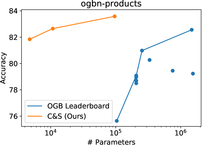
Our C&S framework often requires significantly fewer parameters compared to GNNs or other SOTA solutions. As an example, we plot parameters vs. performance for Products in Figure 2. While having fewer parameters can be useful, the real gain is in faster training time, and our models are typically orders of magnitude faster to train than models with comparable accuracy because we do not use the graph structure for our base predictions. As one example, although our MLP + C&S model based for the Arxiv dataset has a similar number of parameters compared to the GCN + labels method on the OGB leaderboards, our model runs 7 times faster per epoch and converges much faster. In addition, compared to the SOTA for the Products dataset, our framework with a linear base predictor has higher accuracy, trains over 100 times faster, and has 137 times fewer parameters.
We also evaluated our methods on an even larger dataset, the papers100M benchmarks (Hu et al., 2020). Here, we obtain 65.33% using C&S with the Linear model as the base predictor, which out-performs the state-of-the-art on October 1, 2020 (63.29%). Due to computational limits, we could not run exhaustive benchmarks of other GNN models on this dataset.
Our pipeline can also be used to improve the performance of GNNs in general. We applied our error correction and final prediction smoothing to more complex base predictors such as GCNII or GAT. This improves our results on some datasets, including beating SOTA on ogbn-arxiv (Table 5). However, the performance improvements are sometimes only minor, suggesting that big models might be capturing the same signal as our simple C&S framework.
3.4 Performance visualization

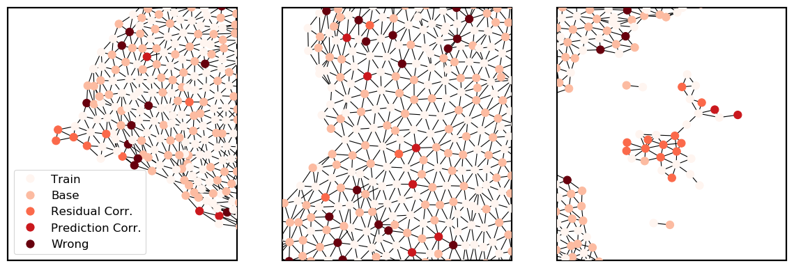
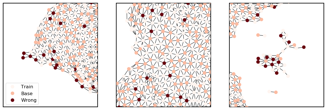
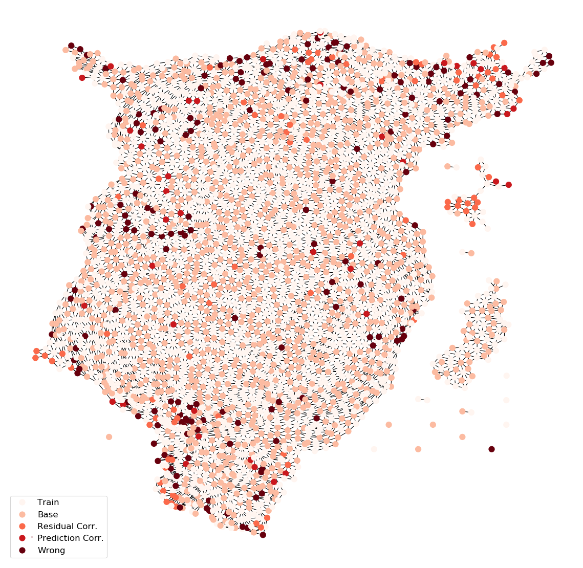
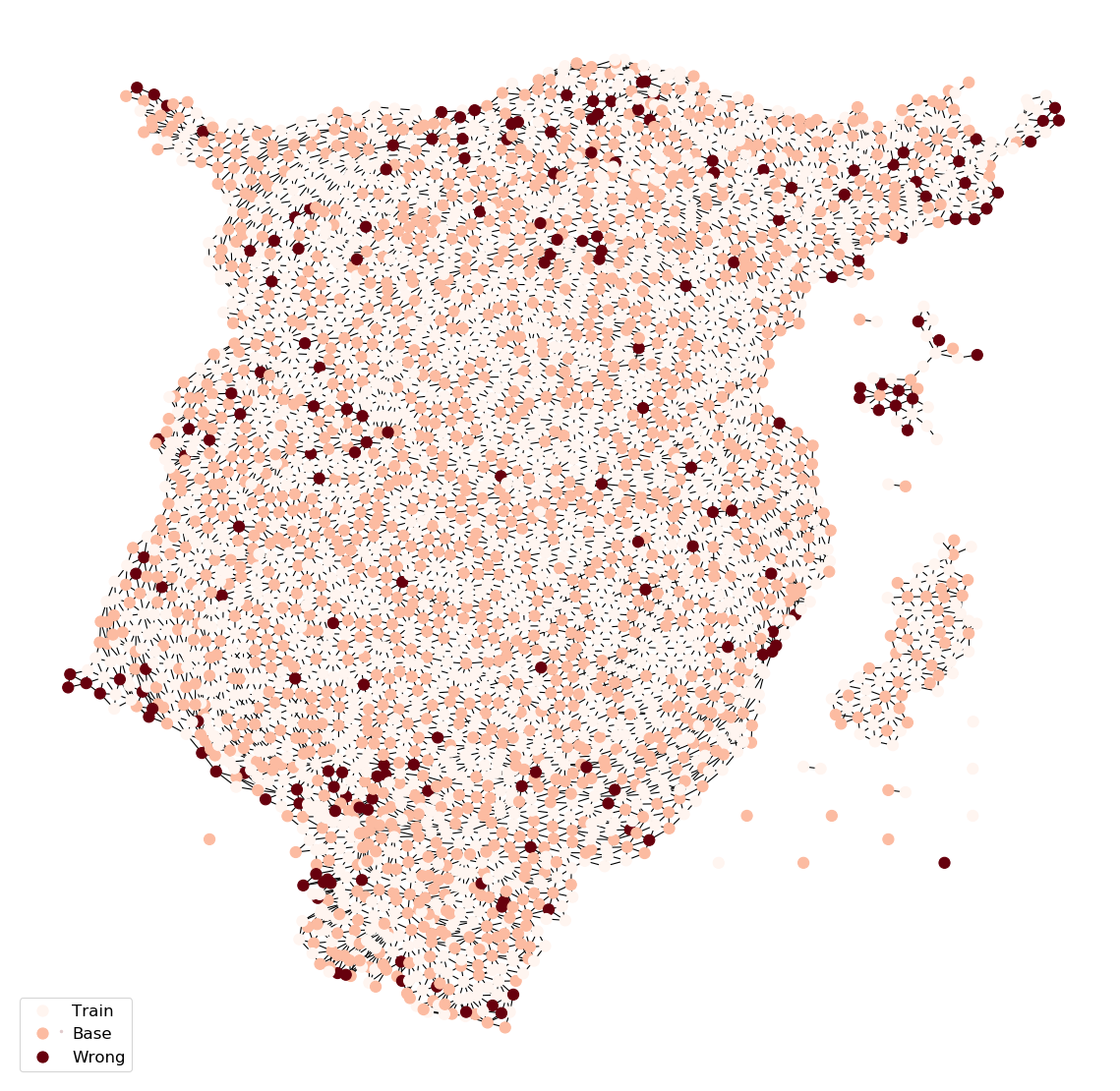
To aid in understanding the performance of our C&S framework, we visualize the predictions on the US County dataset (Figure 3). As expected, the residual error correlation tends to correct nodes where neighboring counties provide relevant information. For example, we see that many errors in the base predictions are corrected by the residual correlation (Figure 3(b), left and right panels) In these cases, which correspond to parts of Texas and Hawaii, the demographic features of the counties are outliers compared to the rest of the country, leading both the linear model and GCN astray. The residual correlation from neighboring counties is able to fix the predictions. We also see that the final prediction correlation will smooth the prediction, as shown in the center panel of Figure 3(b) so that the errors can be fixed based on the correct classification of the neighbors. We observe similar behavior on the Rice31 dataset (see the appendix).
4 Discussion
GNN models are becoming more expressive, more parameterized, and more expensive to train. Our results suggest that we should explore other techniques for improving performance, such as label propagation and feature augmentation. In particular, label propagation and its variants are longstanding, powerful ideas. More directly incorporating them into graph learning models has major benefits, and we have shown that these can lead to both better predictions and faster training.
Acknowledgments. This research was supported by Facebook AI, NSF Award DMS-1830274, ARO Award W911NF19-1-0057, ARO MURI, and JP Morgan Chase & Co.
We would also like to thank the rest of Cornell University Artificial Intelligence for their support and discussion. In addition, we’d like to thank Matthias Fey and Marc Brockschmidt for insightful discussions.
References
- Battaglia et al. (2018) P. Battaglia, Jessica B. Hamrick, V. Bapst, A. Sanchez-Gonzalez, V. Zambaldi, Mateusz Malinowski, Andrea Tacchetti, D. Raposo, Adam Santoro, R. Faulkner, Çaglar Gülçehre, H. Song, A. Ballard, J. Gilmer, G. Dahl, Ashish Vaswani, Kelsey R. Allen, C. Nash, V. Langston, Chris Dyer, N. Heess, Daan Wierstra, Pushmeet Kohli, M. Botvinick, Oriol Vinyals, Y. Li, and Razvan Pascanu. Relational inductive biases, deep learning, and graph networks. ArXiv, abs/1806.01261, 2018.
- Bojchevski et al. (2020) Aleksandar Bojchevski, Johannes Klicpera, Bryan Perozzi, Amol Kapoor, Martin Blais, Benedek Rózemberczki, Michal Lukasik, and Stephan Günnemann. Scaling graph neural networks with approximate pagerank. In Proceedings of the 26th ACM SIGKDD International Conference on Knowledge Discovery and Data Mining, pp. 2464–2473, 2020.
- Chapelle et al. (2003) Olivier Chapelle, Jason Weston, and Bernhard Schölkopf. Cluster kernels for semi-supervised learning. In Advances in neural information processing systems, pp. 601–608, 2003.
- Chaudhuri et al. (2012) Kamalika Chaudhuri, Fan Chung, and Alexander Tsiatas. Spectral clustering of graphs with general degrees in the extended planted partition model. In Conference on Learning Theory, pp. 35–1, 2012.
- Chen et al. (2020) Ming Chen, Zhewei Wei, Zengfeng Huang, Bolin Ding, and Yaliang Li. Simple and deep graph convolutional networks. In Proceedings of the International Conference on Machine Learning, 2020.
- Chin et al. (2019) Alex Chin, Yatong Chen, Kristen M. Altenburger, and Johan Ugander. Decoupled smoothing on graphs. In The World Wide Web Conference, pp. 263–272, 2019.
- Easley & Kleinberg (2010) David Easley and Jon Kleinberg. Networks, crowds, and markets. Cambridge University Press, 2010.
- Eliav & Cohen (2018) Buchnik Eliav and Edith Cohen. Bootstrapped graph diffusions: Exposing the power of nonlinearity. Proceedings of the ACM on Measurement and Analysis of Computing Systems, 2(1):1–19, 2018.
- Fey & Lenssen (2019) Matthias Fey and Jan Eric Lenssen. Fast graph representation learning with pytorch geometric, 2019.
- Gao et al. (2019) Hongchang Gao, Jian Pei, and Heng Huang. Conditional random field enhanced graph convolutional neural networks. In Proceedings of the 25th ACM SIGKDD International Conference on Knowledge Discovery and Data Mining, pp. 276–284, 2019.
- Getoor (2005) Lise Getoor. Link-based classification. In Advanced Methods for Knowledge Discovery from Complex Data, pp. 189–207. Springer, 2005.
- Getoor et al. (2001) Lise Getoor, Nir Friedman, Daphne Koller, and Benjamin Taskar. Learning probabilistic models of relational structure. In International Conference on Machine Learning, pp. 170–177, 2001.
- Gleich & Mahoney (2015) David F Gleich and Michael W Mahoney. Using local spectral methods to robustify graph-based learning algorithms. In Proceedings of the 21th ACM SIGKDD International Conference on Knowledge Discovery and Data Mining, pp. 359–368, 2015.
- Grover & Leskovec (2016) Aditya Grover and J. Leskovec. node2vec: Scalable feature learning for networks. Proceedings of the 22nd ACM SIGKDD International Conference on Knowledge Discovery and Data Mining, 2016.
- Hamilton et al. (2017a) Will Hamilton, Zhitao Ying, and Jure Leskovec. Inductive representation learning on large graphs. In Advances in neural information processing systems, pp. 1024–1034, 2017a.
- Hamilton et al. (2017b) William L Hamilton, Rex Ying, and Jure Leskovec. Representation learning on graphs: Methods and applications. IEEE Data Engineering Bulletin, 2017b.
- Henderson et al. (2011) Keith Henderson, Brian Gallagher, Lei Li, Leman Akoglu, Tina Eliassi-Rad, Hanghang Tong, and Christos Faloutsos. It’s who you know: graph mining using recursive structural features. In Proceedings of the 17th ACM SIGKDD International Conference on Knowledge Discovery and Data Mining, pp. 663–671, 2011.
- Henderson et al. (2012) Keith Henderson, Brian Gallagher, Tina Eliassi-Rad, Hanghang Tong, Sugato Basu, Leman Akoglu, Danai Koutra, Christos Faloutsos, and Lei Li. RolX: structural role extraction & mining in large graphs. In Proceedings of the 18th ACM SIGKDD International Conference on Knowledge Discovery and Data Mining, pp. 1231–1239, 2012.
- Hu et al. (2020) Weihua Hu, M. Fey, M. Zitnik, Yuxiao Dong, H. Ren, Bowen Liu, Michele Catasta, and J. Leskovec. Open graph benchmark: Datasets for machine learning on graphs. ArXiv, abs/2005.00687, 2020.
- Ibrahim & Gleich (2019) Rania Ibrahim and David Gleich. Nonlinear diffusion for community detection and semi-supervised learning. In The World Wide Web Conference, pp. 739–750, 2019.
- Jia & Benson (2020) Junteng Jia and Austin R. Benson. Residual correlation in graph neural network regression. In Proceedings of the 26th ACM SIGKDD International Conference on Knowledge Discovery and Data Mining. ACM Press, 2020.
- Joachims (2003) Thorsten Joachims. Transductive learning via spectral graph partitioning. In Proceedings of the International Conference on Machine Learning, pp. 290–297, 2003.
- Kipf & Welling (2017) Thomas N. Kipf and Max Welling. Semi-supervised classification with graph convolutional networks. In International Conference on Learning Representations, 2017.
- Klicpera et al. (2018) Johannes Klicpera, Aleksandar Bojchevski, and Stephan Günnemann. Predict then propagate: Graph neural networks meet personalized pagerank. In International Conference on Learning Representations, 2018.
- Koutra et al. (2011) Danai Koutra, Tai-You Ke, U Kang, Duen Horng Polo Chau, Hsing-Kuo Kenneth Pao, and Christos Faloutsos. Unifying guilt-by-association approaches: Theorems and fast algorithms. In Joint European Conference on Machine Learning and Knowledge Discovery in Databases, pp. 245–260. Springer, 2011.
- Leskovec et al. (2007) Jure Leskovec, Jon Kleinberg, and Christos Faloutsos. Graph evolution: Densification and shrinking diameters. ACM transactions on Knowledge Discovery from Data, 1(1):2–es, 2007.
- Li et al. (2019) Guohao Li, Matthias Müller, Ali Thabet, and Bernard Ghanem. Deepgcns: Can gcns go as deep as cnns? In The IEEE International Conference on Computer Vision, 2019.
- McInnes et al. (2018) Leland McInnes, John Healy, Nathaniel Saul, and Lukas Großberger. UMAP: Uniform Manifold Approximation and Projection. Journal of Open Source Software, 3(29), 2018.
- McPherson et al. (2001) Miller McPherson, Lynn Smith-Lovin, and James M Cook. Birds of a feather: Homophily in social networks. Annual Review of Sociology, 27(1):415–444, 2001.
- Mernyei & Cangea (2020) P’eter Mernyei and Cătălina Cangea. Wiki-cs: A wikipedia-based benchmark for graph neural networks. ArXiv, abs/2007.02901, 2020.
- Namata et al. (2012) Galileo Namata, Ben London, Lise Getoor, and Bert Huang. Query-driven active surveying for collective classification. In 10th International Workshop on Mining and Learning with Graphs, volume 8, 2012.
- Newman (2003) Mark EJ Newman. Mixing patterns in networks. Physical Review E, 67(2):026126, 2003.
- Paszke et al. (2019) Adam Paszke, Sam Gross, Francisco Massa, Adam Lerer, James Bradbury, Gregory Chanan, Trevor Killeen, Zeming Lin, Natalia Gimelshein, Luca Antiga, Alban Desmaison, Andreas Kopf, Edward Yang, Zachary DeVito, Martin Raison, Alykhan Tejani, Sasank Chilamkurthy, Benoit Steiner, Lu Fang, Junjie Bai, and Soumith Chintala. Pytorch: An imperative style, high-performance deep learning library. In H. Wallach, H. Larochelle, A. Beygelzimer, F. d'Alché-Buc, E. Fox, and R. Garnett (eds.), Advances in Neural Information Processing Systems 32, pp. 8024–8035. Curran Associates, Inc., 2019. URL http://papers.neurips.cc/paper/9015-pytorch-an-imperative-style-high-performance-deep-learning-library.pdf.
- Peel (2017) Leto Peel. Graph-based semi-supervised learning for relational networks. In Proceedings of the 2017 SIAM International Conference on Data Mining, pp. 435–443. SIAM, 2017.
- Qu et al. (2019) Meng Qu, Yoshua Bengio, and Jian Tang. GMNN: Graph markov neural networks. In International Conference on Machine Learning, pp. 5241–5250, 2019.
- Raghavan et al. (2007) Usha Nandini Raghavan, Réka Albert, and Soundar Kumara. Near linear time algorithm to detect community structures in large-scale networks. Physical Review E, 76(3):036106, 2007.
- Rong et al. (2019) Yu Rong, Wenbing Huang, Tingyang Xu, and Junzhou Huang. Dropedge: Towards deep graph convolutional networks on node classification. In International Conference on Learning Representations, 2019.
- Rossi et al. (2020) Emanuele Rossi, Fabrizio Frasca, Ben Chamberlain, Davide Eynard, Michael Bronstein, and Federico Monti. SIGN: Scalable inception graph neural networks. arXiv:2004.11198, 2020.
- Shalizi (2013) Cosma Shalizi. Advanced data analysis from an elementary point of view. Cambridge University Press, 2013.
- Shi et al. (2020) Yunsheng Shi, Zhengjie Huang, Shikun Feng, and Yu Sun. Masked label prediction: Unified massage passing model for semi-supervised classification. arXiv:2009.03509, 2020.
- Traud et al. (2012) Amanda L Traud, Peter J Mucha, and Mason A Porter. Social structure of facebook networks. Physica A: Statistical Mechanics and its Applications, 391(16):4165–4180, 2012.
- Tudisco et al. (2020) Francesco Tudisco, Austin R Benson, and Konstantin Prokopchik. Nonlinear higher-order label spreading. arXiv:2006.04762, 2020.
- Veličković et al. (2018) Petar Veličković, Guillem Cucurull, Arantxa Casanova, Adriana Romero, Pietro Liò, and Yoshua Bengio. Graph Attention Networks. International Conference on Learning Representations, 2018.
- Wang & Zhang (2007) Fei Wang and Changshui Zhang. Label propagation through linear neighborhoods. IEEE Transactions on Knowledge and Data Engineering, 20(1):55–67, 2007.
- Wang & Leskovec (2020) Hongwei Wang and Jure Leskovec. Unifying graph convolutional neural networks and label propagation. arXiv:2002.06755, 2020.
- Wu et al. (2019) Felix Wu, Amauri Souza, Tianyi Zhang, Christopher Fifty, Tao Yu, and Kilian Weinberger. Simplifying graph convolutional networks. In Proceedings of the 36th International Conference on Machine Learning, pp. 6861–6871. PMLR, 2019.
- Wu et al. (2020) Zonghan Wu, Shirui Pan, Fengwen Chen, Guodong Long, C. Zhang, and Philip S. Yu. A comprehensive survey on graph neural networks. IEEE Transactions on Neural Networks and Learning Systems, 2020.
- Xu et al. (2018) Keyulu Xu, Weihua Hu, Jure Leskovec, and Stefanie Jegelka. How powerful are graph neural networks? In International Conference on Learning Representations, 2018.
- Yang et al. (2016) Zhilin Yang, William Cohen, and Ruslan Salakhudinov. Revisiting semi-supervised learning with graph embeddings. In International conference on machine learning, pp. 40–48, 2016.
- Yin et al. (2017) Hao Yin, Austin R Benson, Jure Leskovec, and David F Gleich. Local higher-order graph clustering. In Proceedings of the 23rd ACM SIGKDD International Conference on Knowledge Discovery and Data Mining, pp. 555–564, 2017.
- Zeng et al. (2019) Hanqing Zeng, Hongkuan Zhou, Ajitesh Srivastava, Rajgopal Kannan, and Viktor Prasanna. GraphSAINT: Graph sampling based inductive learning method. In International Conference on Learning Representations, 2019.
- Zhang & Rohe (2018) Yilin Zhang and Karl Rohe. Understanding regularized spectral clustering via graph conductance. In Advances in Neural Information Processing Systems, pp. 10631–10640, 2018.
- Zhou et al. (2004) Dengyong Zhou, Olivier Bousquet, Thomas N Lal, Jason Weston, and Bernhard Schölkopf. Learning with local and global consistency. In Advances in neural information processing systems, pp. 321–328, 2004.
- Zhu et al. (2003) Xiaojin Zhu, Zoubin Ghahramani, and J. Lafferty. Semi-supervised learning using gaussian fields and harmonic functions. In Proceedings of the International Conference on Machine Learning, 2003.
- Zhu (2005) Xiaojin Jerry Zhu. Semi-supervised learning literature survey. Technical report, University of Wisconsin-Madison Department of Computer Sciences, 2005.
Appendix A Model Details
Here we provide some more details on the models that we use. In all cases we use the Adam optimizer and tune the learning rate. We follow the models and hyperparameters provided in OGB (Hu et al., 2020) and wikiCS (Mernyei & Cangea, 2020) and manually tune some hyperparameters on the validation data for the potential better performance.
For our MLPs, every linear layer is followed by batch normalization, ReLU activation, and 0.5 dropout. The other parameters depend on the dataset as follows.
-
•
OGB datasets: 3 layers and 256 hidden channels with learning rate equal to 0.01.
- •
-
•
wikiCS: 3 layers and 256 hidden channels with learning rate equal to 0.005.
- •
Most of the “State-of-the-Art” models are taken from benchmark datasets. We determined SOTA for Email, US County, and Rice31 based on all other models used in the paper. The best performing SOTA baselines were as follows. For Email, GCNII with 5 layers, 256 hidden channels, learning rate equal to 0.01. For US County, GCNII with 8 layers, 256 hidden channels, learning rate equal to 0.03. For Rice31, we reused our base GCN architecture and trained it over spectral and node2vec embeddings. This significantly outperformed the other GNN variants.
Appendix B Performance Results with only Residual Correlation
Table 6 shows results when using residual correlation but not smoothing in the final predictions, i.e., just the “C” step of our C&S framework. The results indicate both the label propagation steps matter significantly for the final improvements.
| Methods | Base Model | Arxiv | Products | Cora | Citeseer | Pubmed |
|---|---|---|---|---|---|---|
| Plain Linear | 66.89 | 74.63 | 79.56 | 72.56 | 88.56 | |
| Autoscale | Linear | 71.52 | 70.93 | 79.08 | 70.77 | 88.84 |
| MLP | 71.97 | 69.85 | 74.11 | 71.78 | 87.35 | |
| Plain Linear | 65.62 | 80.97 | 76.48 | 70.48 | 87.52 | |
| FDiff- | Linear | 70.26 | 73.89 | 79.32 | 70.53 | 84.47 |
| scale | MLP | 71.55 | 72.72 | 74.36 | 71.45 | 86.97 |
| Methods | Base Model | Rice31 | US County | wikiCS | ||
| Plain Linear | — | 43.97 | 82.60 | 77.49 | ||
| Autoscale | Linear | 73.39 | 86.19 | 84.08 | 74.06 | |
| MLP | 71.64 | 84.61 | 88.83 | 78.72 | ||
| Plain Linear | — | 72.44 | 87.16 | 75.98 | ||
| FDiff- | Linear | 71.31 | 85.22 | 88.27 | 73.86 | |
| scale | MLP | 72.59 | 85.42 | 89.62 | 78.40 |
Appendix C Additional visualization
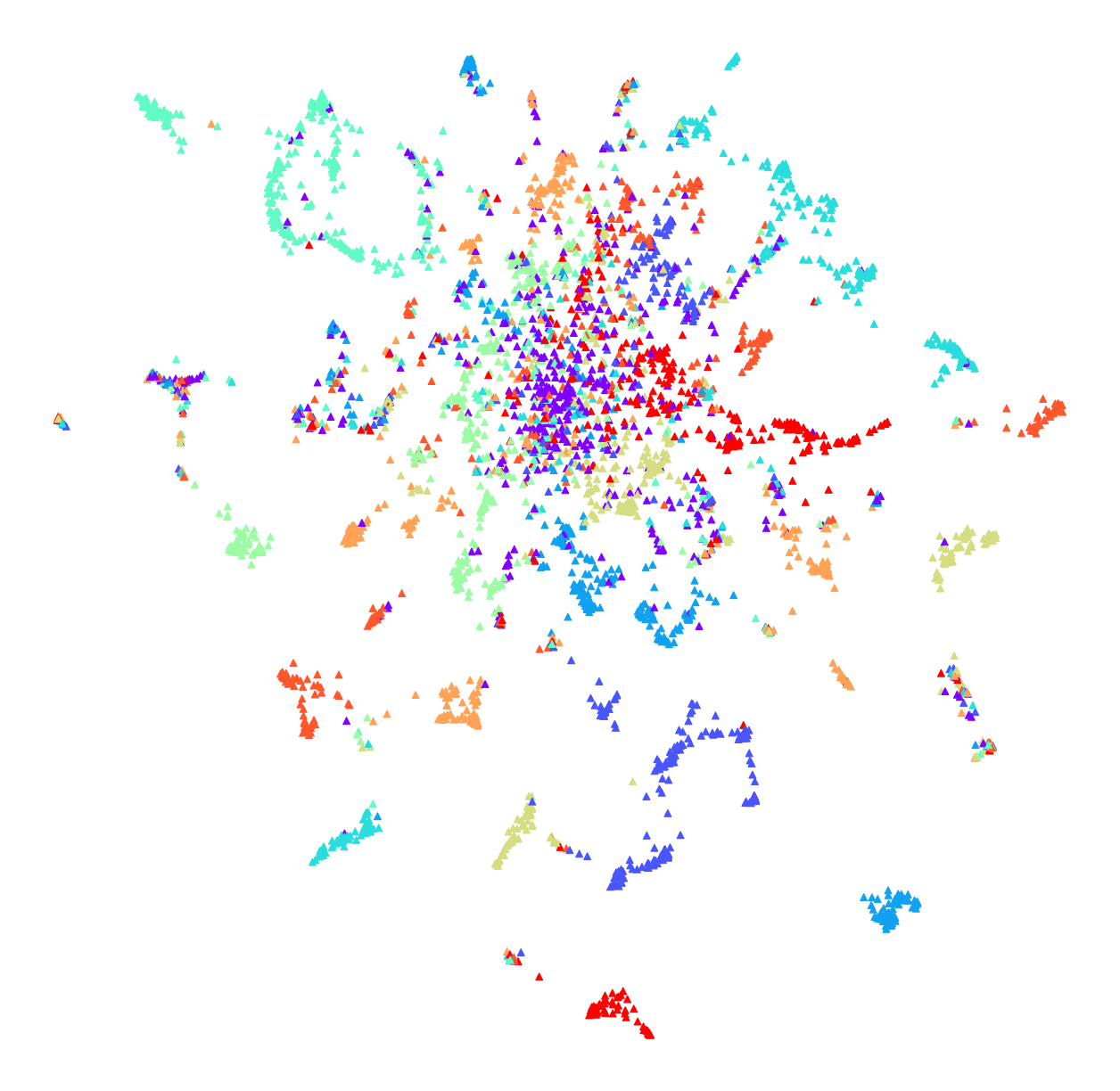
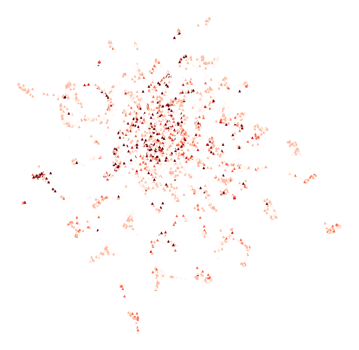
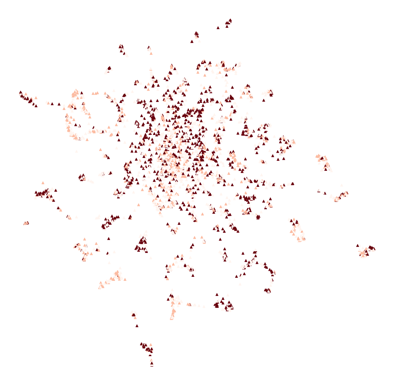
Visualizations of the US County and Rice31 dataset are shown in Figures 4, 5, 6, 7, 8 and 9. The Rice31 visualization is generated by projecting the 128-dimensional spectral embedding used in the main text down to two dimensions with UMAP (McInnes et al., 2018).
