A Linear Quadratic Partially Observed Stackelberg Stochastic Differential Game with Applications thanks: This work is supported by National Key R&D Program of China (Grant No. 2018YFB1305400), National Natural Science Foundations of China (Grant Nos. 11971266, 11831010, 11571205), and Shandong Provincial Natural Science Foundations (Grant Nos. ZR2020ZD24, ZR2019ZD42).

Yueyang Zheng , Jingtao Shi School of Mathematics, Shandong University, Jinan 250100, P.R.China, E-mail: zhengyueyang0106@163.comCorresponding author. School of Mathematics, Shandong University, Jinan 250100, P.R.China, E-mail: shijingtao@sdu.edu.cn

Abstract: This paper is concerned with a linear-quadratic partially observed Stackelberg stochastic differential game with correlated state and observation noises, where the diffusion coefficient does not contain the control variable and the control set is not necessarily convex. Both the leader and the follower have their own observation equations, and the information filtration available to the leader is contained in that to the follower. By spike variational, state decomposition and backward separation techniques, necessary and sufficient conditions of the Stackelberg equilibrium points are derived. In the follower’s problem, the state estimation feedback of optimal control can be represented by a forward-backward stochastic differential filtering equation and some Riccati equation. In the leader’s problem, via the innovation process, the state estimation feedback of optimal control is represented by a stochastic differential filtering equation, a semi-martingale process and three high-dimensional Riccati equations. At the same time, the uniqueness and existence of solutions to adjoint equations can be guaranteed by a new combined idea, and a kind of fully coupled forward-backward stochastic differential equations with filtering is studied as a by-product. Then we give explicit expressions of Stackelberg equilibrium points in a special case. As a practical application, an inspiring dynamic advertising problem with asymmetric information is studied, and the effectiveness and reasonability of the theoretical result is illustrated by numerical simulations. Moreover, the relationship between optimal control, state estimate and some practical parameters is analyzed in detail.

Keywords: Stackelberg stochastic differential game, leader and follower, partial observation, linear-quadratic control, state decomposition, backward separation, stochastic filtering, Stackelberg equilibrium point

Mathematics Subject Classification: 93E20, 49K45, 49N10, 49N70, 60H10

1 Introduction

Among various dynamic games, the Stackelberg game was introduced firstly by Stackelberg [35], which is a kind of hierarchical noncooperative game (Başar and Olsder [1]). The Stackelberg game is also know as the leader-follower game, whose economic background can be derived from some markets where certain companies have advantages of domination over others. In the Stackelberg game, there are usually two players with asymmetric roles, one follower and one leader. The leader claims his/her strategy in advance, and the follower, considering the given leader’s strategy, makes an instantaneous reaction by optimizing his/her cost functional. Then, by taking the rational response of the follower into account, the leader would like to seek an optimal strategy to optimize his/her cost functional. Therefore, one player must make a decision after the other player’s decision is made. Since its meaningful structure and background, the Stackelberg game has received substantial interest. Especially, the leader-follower’s feature can be applied in many aspects, such as the newsvendor/wholesaler problem (Øksendal et al. [28]), the optimal reinsurance problem (Chen and Shen [8]), the operations management and marketing channel problem (Li and Sethi [19]) and the principal-agent/optimal contract problem (Cvitanić and Zhang [9]).

In the past decades, there have been a great deal of significant works on this issue. Let us mention a few. First, Castanon and Athans [7] studied an LQ stochastic dynamic Stackelberg strategies in the early, and obtained a feedback Stackelberg solution for two-person nonzero sum game. An indefinite LQ leader-follower stochastic differential game with random coefficients and control-dependent diffusion was studied by Yong [51]. Forward-backward stochastic differential equations (FBSDEs for short) and Riccati equations are applied to obtain the state feedback representation of the open-loop Stackelberg equilibrium points. Başar et al. [2] introduced the notion of mixed leadership in nonzero-sum differential games where one player could act as both leader and follower, depending on the control variable. Bensoussan et al. [6] introduced several solution concepts in terms of the players’ information sets, and derived the maximum principle for the leader’s global Stackelberg solution under the adapted closed-loop memoryless information structure. Mukaidani and Xu [27] investigated the Stackelberg games for linear stochastic systems governed by Itô differential equations with multiple followers. The Stackelberg strategies, obtained by using sets of cross-coupled algebraic nonlinear matrix equations, are developed under two different settings: the followers act either cooperatively to attain Pareto optimality or non-cooperatively to arrive at a Nash equilibrium. Xu and Zhang [49] and Xu et al. [48] investigated the LQ Stackelberg differential games with time delay. Li and Yu [18] proved the solvability of a kind of coupled FBSDEs with a multilevel self-similar domination-monotonicity structure, then it is used to characterize the unique equilibrium of an LQ generalized Stackelberg stochastic differential game with hierarchy in a closed form. Moon and Başar [26] considered the LQ mean-field Stackelberg differential game with the adapted open-loop information structure of the leader where the N𝑁N followers play a Nash game. Lin et al. [24] studied the open-loop LQ Stackelberg game of the mean-field stochastic systems and obtained the feedback representation form involving the new state and its mean. Du and Wu [11] investigated an LQ Stackelberg game of mean-field backward stochastic differential equations (BSDEs for short). Zheng and Shi [55] researched the Stackelberg game of BSDEs with complete information. Bensoussan et al. [5] characterized the feedback equilibrium of a general infinite horizon Stackelberg-Nash differential game where the roles of the players are mixed. Recently, Huang et al. [13] studied a controlled linear-quadratic-Gaussian large population system combining major leader, minor leaders and minor followers. The Stackelberg-Nash-Cournot (SNC for short) approximate equilibrium is derived from the combination of a major-minor mean-field game and a leader-follower Stackelberg game, and the feedback form of the SNC approximate equilibrium strategy is obtained via some coupled Riccati equations. Feng et al. [12] considered the LQ Stackelberg game of BSDEs with constraints.

Noticing all the Stackelberg game considered in the above are set in the complete information background. In other word, both the leader and the follower can observe the state process of the stochastic system directly, which, however, is impractical in reality. Actually, both of them can only acquire partial information because of the information-delay, market competition, private information and limitation policy by the government. Therefore, it is necessary to study the Stackelberg game with partial and asymmetric information. There exist a number of works on this issue, very recently. Shi et al. [31, 32] studied the Stackelberg stochastic differential game and introduced a new explanation for the asymmetric information feature, that the information available to the follower is based on the some sub-σ𝜎\sigma-algebra of that available to the leader. Shi et al. [33] investigated the LQ Stackelberg stochastic differential game with overlapping information, where the follower’s and the leader’s information have some joint part, while they have no inclusion relations. Wang et al. [37] discussed an asymmetric information mean-field type LQ Stackelberg stochastic differential game with one leader and two followers. Zheng and Shi [56] investigated a LQ Stackelberg game of BSDEs with partial information, where the information of the leader is a sub-σ𝜎\sigma-algebra of that of the follower.

However, the asymmetric information feature in the above literatures only shows that all the partial information available to the leader and the follower are generated by the noisy processes - standard Brownian motions. In reality, the player’s available information usually comes from the observation process. For example, in the financial market, the investor can only observe the security prices. Therefore, the investors would like to make their portfolio selection based on the information filtration generated by the security prices process (Xiong and Zhou [46]). The essential works associated with the partially observed problem is the filtering estimate problem which consists of two processes: the signal process and the observation process. Then the aim of the filtering theory is to estimate the signal process based on the information generated by the observation processes (Liptser and Shiryayev [25], Bensoussan [3], Xiong [45] and Wang and Wu [38]). Partially observed optimal control and differential game problems have been studied by many researchers, such as Li and Tang [20], Tang [36], Wang and Wu [39], Huang et al. [14], Wu [43], Shi and Wu [34], Wang et al. [40, 41, 42], Wu and Zhuang [44], Xiong et al. [47]. Up to now, few studies have focussed on the partially observed Stackelberg differential game. Li et al. [21] derived the necessary condition of this leader-follower stochastic differential game under a partially observed information where the controlled system equation and the observation equation are looked as the equality constraints. Zheng and Shi [57] studied a Stackelberg stochastic differential game with asymmetric noisy observation where the follower cannot observe the state process directly, while the leader can completely observe it. Very recently, Li et al. [22] investigated an LQ Gaussian Stackelberg stochastic differential game under asymmetric information. Two decision makers implement control strategies using different information patterns: The follower uses its observation information to design its strategy, whereas the leader implements its strategy using global information.

Our work distinguishes itself from the existing literature in the following aspects:

(1) To our best acknowledge, there is no previous research on the LQ partially observed Stackelberg stochastic differential game using the state decomposition and backward separation techniques, where the leader and the follower have their own observation equations different from each other. For technical need, in this paper we assume that the information filtration available to the leader is included in that available to the follower, compared to Li et al. [21] where both the leader and the follower’s controls are adapted to the filtration generated by the same observation process and Li et al. [22], Zheng and Shi [57] where the information available to the leader is more than that available to the follower. However, it is not a trivial setting on account of the technical difficulty appeared in the follower’s part when utilizing the state decomposition technique. First, different from Xiong et al. [47], in which the Girsanov’s theorem and measure transformation method are used, in this paper we apply state decomposition and backward separation techniques from Wang et al. [41], although in [47] two observation equations are also considered. Secondly, different from Wu and Zhuang [44] where the controls of two players are adapted to the filtration generated by the same observation process, therefore, the similar result can be obtained easily as Lemma 2.1 in [41]. Different from [41] in which they consider the control problem, in this paper the Stackelberg game is researched and it fails to proceed in the follower’s part without our new assumption (Lemma 3.1), since the two control variables appears in the hierarchical structure. Moreover, many practical examples, such as the market channel and operations management problems, can be applied to verify the assumption’s reasonability.

(2) For characterizing the adaptation and relationship of these filtrations well appearing in this paper, in Remark 2.2, we make a detailed analysis for the partially observed problem, especially for the essence of observation equations. More importantly, we compare it with the partial information problem which should be another case, and show their intrinsic distinctions.

(3) We need to solve a partially observed optimal control problem of FBSDFEs in the leader’s problem, after dealing with the partially observed optimal control problem of the follower. However, different from all the existing literatures of Stackelberg stochastic differential game with partial information, in which the state equation’s driven noises of the leader only contains the independent tsubscript𝑡\mathcal{F}_{t}-standard Brownian motions, in this paper when observing the equations (3.35) and (3.49) (or (3.51)), the appearance of a new tY1superscriptsubscript𝑡subscript𝑌1\mathcal{F}_{t}^{Y_{1}}-Brownian motion W~~𝑊\widetilde{W} (the innovation process) makes our leader’s problem become an entirely new problem which is not investigated before. Therefore, we have to consider a kind of state equations with the fact that W~~𝑊\widetilde{W} is not independent of the standard Brownian motions W𝑊W or W¯¯𝑊\bar{W}. Moreover, the foremost issue in this step, is to guarantee the uniqueness and existence of solution to this kind of equations. We solve this difficult problem by a new combined idea from Yong [51] and Lim and Zhou [23].

(4) It is worth noting that we are supposed to give the existence and uniqueness of solution to (3.53) with three different Brownian motions first, then decouple it for obtaining the state estimation feedback of optimal control. Motivated by the usual step and the classical method in Peng and Wu [30], we study a kind of fully coupled FBSDEs with filtering which can be regarded as a special case of (3.53), and get the existence and uniqueness of their solutions by constructing a contraction mapping and using fixed-point theorem. However, we fail to prove the unique solvability of the FBSDFE (3.53), because it is not only a fully coupled one, but also contains two kinds of filtering form, (X^,Y^)^𝑋^𝑌(\hat{X},\hat{Y}) and (Xˇ,Yˇ)ˇ𝑋ˇ𝑌(\check{X},\check{Y}). Therefore, we can not solve it directly by existing methods. Fortunately, we find an idea to obtain its unique solvability as follows: we first obtain the existence of solution to (3.53) by decoupling technique as usual, and further guarantee that the solution is indeed unique inspired by the method in [23]. More importantly, the existence and uniqueness of adjoint equations (3.41) and (3.42) in the leader’s problem should also be given. In fact, we also have difficult in dealing with it because of the existence of W,W¯,W~𝑊¯𝑊~𝑊W,\bar{W},\widetilde{W}. But we can observe that the adjoint equations are related to (3.53), therefore, we can solve (3.53) first and consequently ensure the unique solvability of (3.41) and (3.42).

(5) The semi-martingale ΦΦ\Phi of (3.76) is introduced in the relation (3.62) between Y𝑌Y and X,X^,Xˇ𝑋^𝑋ˇ𝑋X,\hat{X},\check{X}. However, different from [21], the ΦΦ\Phi is not only used to “absorb” the W~~𝑊\widetilde{W} in the filtering equations (3.66), but also to explain the reasonable existence of W~~𝑊\widetilde{W} appeared in the leader’s state and adjoint equations as a driven noise which is control-independent. Moreover, for obtaining the state estimation feedback of the Stackelberg equilibrium point, we make a detailed analysis on the filtrations generated by Y1,Y2subscript𝑌1subscript𝑌2Y_{1},Y_{2} and W~~𝑊\widetilde{W}, respectively, and discuss their relationships in order to facilitate the filtering problem.

(6) For giving an explicit form for Stackelberg equilibrium points, we reduce the original problem to a special one under some conditions and obtain some explicit expressions. Then an application to the dynamic advertising problem with asymmetric information is studied, which extends an example in Jorgensen et al. [17] to the stochastic case with partially observable information. This inspiring motivation is an excellent explanation for the condition that both the leader and the follower can not observe the complete information, and the information available to the leader is less than that available to the follower. Its numerical simulation is also given to verify the effectiveness of the proposed theoretical results, moreover, we also analyze the relationship between the optimal advertising effort, brand image and its estimate and some practical parameters.

The rest of this article is organized as follows. In Section 2, we formulate an LQ partially observed Stackelberg stochastic differential game model and adopt the state decomposition technique to deal with it. In Section 3, the necessary and sufficient conditions of the partially observed optimal control problem of the follower are given by using the backward separation technique, and the state estimation feedback representation is obtained via an FBSDFE and one Riccati equation in Section 3.1. In Section 3.2, we prove the maximum principle of the partially observed optimal control problem of FBSDFEs of the leader, and give the sufficient condition of the optimal control. For obtaining the state estimate feedback, we first obtain the unique solvability of leader’s state in a form of FBSDFE by a new combined idea. Then the optimal control can be represented by an SDFE, three high-dimensional Riccati equations and a semi-martingale. In Section 4, we focus on a special partially observed case and give the explicit expressions of Stackelberg equilibrium points. In Section 5, a practical application to the dynamic advertising problem is studied, and its numerical simulation is given to illustrate the effectiveness of the proposed theoretical results. Moreover, the relationship between the Stackelberg equilibrium points, state estimate and some practical parameters is also discussed. Finally, some concluding remarks are list in Section 6.

2 Problem Formulation

Let T>0𝑇0T>0 be fixed. Consider a complete filtered probability space (Ω,,(tW,W¯)0tT,)Ωsubscriptsuperscriptsubscript𝑡𝑊¯𝑊0𝑡𝑇(\Omega,\mathcal{F},(\mathcal{F}_{t}^{W,\bar{W}})_{0\leq t\leq T},\mathbb{P}) and two one-dimensional independent standard Brownian motions W()𝑊W(\cdot) and W¯()¯𝑊\bar{W}(\cdot) defined in 2superscript2\mathbb{R}^{2} with W(0)=W¯(0)=0𝑊0¯𝑊00W(0)=\bar{W}(0)=0, which generates the filtration tW,W¯:=σ{W(r),W¯(r):0rt}assignsuperscriptsubscript𝑡𝑊¯𝑊𝜎conditional-set𝑊𝑟¯𝑊𝑟0𝑟𝑡\mathcal{F}_{t}^{W,\bar{W}}:=\sigma\{W(r),\bar{W}(r):0\leq r\leq t\} augmented by all the \mathbb{P}-null sets in \mathcal{F}. We set ttW,W¯subscript𝑡superscriptsubscript𝑡𝑊¯𝑊\mathcal{F}_{t}\equiv\mathcal{F}_{t}^{W,\bar{W}} if there is no ambiguity. In this paper, LT2(Ω,)superscriptsubscript𝐿subscript𝑇2ΩL_{\mathcal{F}_{T}}^{2}(\Omega,\mathbb{R}) denotes the set of \mathbb{R}-valued, Tsubscript𝑇\mathcal{F}_{T}-measurable, square-integrable random variables, L2(0,T;)subscriptsuperscript𝐿20𝑇L^{2}_{\mathcal{F}}(0,T;\mathbb{R}) denotes the set of \mathbb{R}-valued, tsubscript𝑡\mathcal{F}_{t}-adapted, square integrable processes on [0,T]0𝑇[0,T], and L(0,T;)superscript𝐿0𝑇L^{\infty}(0,T;\mathbb{R}) denotes the set of \mathbb{R}-valued, bounded functions on [0,T]0𝑇[0,T]. For any stochastic process Δ():[0,T]×Ω:Δ0𝑇Ω\Delta(\cdot):[0,T]\times\Omega\rightarrow\mathbb{R}, tΔsuperscriptsubscript𝑡Δ\mathcal{F}_{t}^{\Delta} denote the filtration generated by stochastic process Δ()Δ\Delta(\cdot) in [0,t]0𝑡[0,t], that is, tΔ:=σ{Δ(r):0rt}assignsuperscriptsubscript𝑡Δ𝜎conditional-setΔ𝑟0𝑟𝑡\mathcal{F}_{t}^{\Delta}:=\sigma\{\Delta(r):0\leq r\leq t\}.

We consider the following controlled linear stochastic differential equation (SDE for short):

{dxv1,v2(t)=[A(t)xv1,v2(t)+B1(t)v1(t)+B2(t)v2(t)+α(t)]dt+c(t)dW(t)+c¯(t)dW¯(t),t[0,T],xv1,v2(0)=x0,\left\{\begin{aligned} dx^{v_{1},v_{2}}(t)&=\big{[}A(t)x^{v_{1},v_{2}}(t)+B_{1}(t)v_{1}(t)+B_{2}(t)v_{2}(t)+\alpha(t)\big{]}dt\\ &\quad+c(t)dW(t)+\bar{c}(t)d\bar{W}(t),\ t\in[0,T],\\ x^{v_{1},v_{2}}(0)&=x_{0},\end{aligned}\right. (2.1)

and the observation processes of the follower and the leader satisfy

{dY1v1,v2(t)=[f1(t)xv1,v2(t)+g(t)]dt+dW(t),t[0,T],Y1v1,v2(0)=0,\left\{\begin{aligned} dY_{1}^{v_{1},v_{2}}(t)&=\big{[}f_{1}(t)x^{v_{1},v_{2}}(t)+g(t)\big{]}dt+dW(t),\ t\in[0,T],\\ Y_{1}^{v_{1},v_{2}}(0)&=0,\end{aligned}\right. (2.2)
{dY2v2(t)=[f2(t)+v2(t)]dt+dW(t),t[0,T],Y2v2(0)=0,\left\{\begin{aligned} dY_{2}^{v_{2}}(t)&=\big{[}f_{2}(t)+v_{2}(t)\big{]}dt+dW(t),\ t\in[0,T],\\ Y_{2}^{v_{2}}(0)&=0,\end{aligned}\right. (2.3)

respectively. Here (v1(),v2())2subscript𝑣1subscript𝑣2superscript2(v_{1}(\cdot),v_{2}(\cdot))\in\mathbb{R}^{2} are the control process pair of the follower and the leader, (xv1,v2(),Y1v1,v2())2superscript𝑥subscript𝑣1subscript𝑣2superscriptsubscript𝑌1subscript𝑣1subscript𝑣2superscript2(x^{v_{1},v_{2}}(\cdot),Y_{1}^{v_{1},v_{2}}(\cdot))\in\mathbb{R}^{2} are the state process and corresponding follower’s observation process related to (v1(),v2())subscript𝑣1subscript𝑣2(v_{1}(\cdot),v_{2}(\cdot)), and Y2v2()superscriptsubscript𝑌2subscript𝑣2Y_{2}^{v_{2}}(\cdot)\in\mathbb{R} is the leader’s observation process independent of the control v1()subscript𝑣1v_{1}(\cdot).

Remark 2.1.

Observing the leader’s observation equation (2.3), we can see that the drift term, which is free of xv1,v2superscript𝑥subscript𝑣1subscript𝑣2x^{v_{1},v_{2}}, is chosen by the leader, then it is easy to check that tY2v2=tWsuperscriptsubscript𝑡superscriptsubscript𝑌2subscript𝑣2superscriptsubscript𝑡𝑊\mathcal{F}_{t}^{Y_{2}^{v_{2}}}=\mathcal{F}_{t}^{W}. In other words, the observation filtration is influenced by the control process v2()subscript𝑣2v_{2}(\cdot) in form, but the circular dependence between Y2v2()superscriptsubscript𝑌2subscript𝑣2Y_{2}^{v_{2}}(\cdot) and v2()subscript𝑣2v_{2}(\cdot) disappear because of the fact v2()tY2v2=tWsubscript𝑣2superscriptsubscript𝑡superscriptsubscript𝑌2subscript𝑣2superscriptsubscript𝑡𝑊v_{2}(\cdot)\in\mathcal{F}_{t}^{Y_{2}^{v_{2}}}=\mathcal{F}_{t}^{W}. Moreover, due to the state decomposition in the following, (2.10) implies tY20=tWsuperscriptsubscript𝑡superscriptsubscript𝑌20superscriptsubscript𝑡𝑊\mathcal{F}_{t}^{Y_{2}^{0}}=\mathcal{F}_{t}^{W}. Therefore, we get an important result that tY2v2=tY20=tWsuperscriptsubscript𝑡superscriptsubscript𝑌2subscript𝑣2superscriptsubscript𝑡superscriptsubscript𝑌20superscriptsubscript𝑡𝑊\mathcal{F}_{t}^{Y_{2}^{v_{2}}}=\mathcal{F}_{t}^{Y_{2}^{0}}=\mathcal{F}_{t}^{W}, which is one of the main conclusion used many times in the following discussion.

Remark 2.2.

We note that the leader’s observation equation of Y2v2()superscriptsubscript𝑌2subscript𝑣2Y_{2}^{v_{2}}(\cdot) is not general enough. Indeed, we consider that the drift term of (2.3) is not related to the state variable xv1,v2()superscript𝑥subscript𝑣1subscript𝑣2x^{v_{1},v_{2}}(\cdot), but is related to the leader’s control variable v2()subscript𝑣2v_{2}(\cdot) directly. It is necessary to explain why we set the form and illustrate the difficulties with the general form. If we consider the general form of Y2()subscript𝑌2Y_{2}(\cdot) as the following

{dY2v1,v2(t)=[f2(t)xv1,v2(t)+g2(t)]dt+dW(t),t[0,T],Y2v1,v2(0)=0,\left\{\begin{aligned} dY_{2}^{v_{1},v_{2}}(t)&=\big{[}f_{2}(t)x^{v_{1},v_{2}}(t)+g_{2}(t)\big{]}dt+dW(t),\ t\in[0,T],\\ Y_{2}^{v_{1},v_{2}}(0)&=0,\end{aligned}\right. (2.4)

and we separate Y2v1,v2()superscriptsubscript𝑌2subscript𝑣1subscript𝑣2Y_{2}^{v_{1},v_{2}}(\cdot) into two parts:

{dY20(t)=f2(t)x0(t)dt+dW(t),t[0,T],Y20(0)=0,\left\{\begin{aligned} dY_{2}^{0}(t)&=f_{2}(t)x^{0}(t)dt+dW(t),\ t\in[0,T],\\ Y_{2}^{0}(0)&=0,\end{aligned}\right. (2.5)

and

{dY21(t)=[f2(t)x1(t)+g2(t)]dt,t[0,T],Y21(0)=0.\left\{\begin{aligned} dY_{2}^{1}(t)&=\big{[}f_{2}(t)x^{1}(t)+g_{2}(t)\big{]}dt,\ t\in[0,T],\\ Y_{2}^{1}(0)&=0.\end{aligned}\right. (2.6)

Observing the above equations (2.5) and (2.6), and combining the separated equations (2.7), (2.8), (2.9), (2.11), (2.12) in the following, two challenging problems arise naturally in Section 3.2. The first one is the appearance of another new tY2v¯1,v2superscriptsubscript𝑡superscriptsubscript𝑌2subscript¯𝑣1subscript𝑣2\mathcal{F}_{t}^{Y_{2}^{\bar{v}_{1},v_{2}}}-adapted Brownian motion W~2subscript~𝑊2\widetilde{W}_{2} which is also called the innovation process when we calculate the filtering equations with respect to tY2v¯1,v2superscriptsubscript𝑡superscriptsubscript𝑌2subscript¯𝑣1subscript𝑣2\mathcal{F}_{t}^{Y_{2}^{\bar{v}_{1},v_{2}}} in the leader’s problem, which make the problem more complicated taking the W,W¯,W~𝑊¯𝑊~𝑊W,\bar{W},\widetilde{W} and W~2subscript~𝑊2\widetilde{W}_{2} into account. The second one is that, under the assumption in Lemma 3.1, we fail to guarantee that tY2v¯1,v2=tY20superscriptsubscript𝑡superscriptsubscript𝑌2subscript¯𝑣1subscript𝑣2superscriptsubscript𝑡superscriptsubscript𝑌20\mathcal{F}_{t}^{Y_{2}^{\bar{v}_{1},v_{2}}}=\mathcal{F}_{t}^{Y_{2}^{0}} holds which make it impossible for us to overcome the circular dependency between v2subscript𝑣2v_{2} and tY2v¯1,v2superscriptsubscript𝑡superscriptsubscript𝑌2subscript¯𝑣1subscript𝑣2\mathcal{F}_{t}^{Y_{2}^{\bar{v}_{1},v_{2}}}.

From what has been discussed above, we consider the form in (2.3) which is convenient to study the leader’s problem although the circulation still exists.

Now some assumptions are needed.

(A1) A(),B1(),B2(),α(),c(),c¯(),f1(),f2()𝐴subscript𝐵1subscript𝐵2𝛼𝑐¯𝑐subscript𝑓1subscript𝑓2A(\cdot),B_{1}(\cdot),B_{2}(\cdot),\alpha(\cdot),c(\cdot),\bar{c}(\cdot),f_{1}(\cdot),f_{2}(\cdot) and g()𝑔g(\cdot) are uniformly bounded, deterministic functions. x0subscript𝑥0x_{0} is a constant.

Under (𝐀𝟏)𝐀𝟏\bf(A1), for any given v1()L2(0,T;)subscript𝑣1subscriptsuperscript𝐿20𝑇v_{1}(\cdot)\in L^{2}_{\mathcal{F}}(0,T;\mathbb{R}) and v2()L2(0,T;)subscript𝑣2subscriptsuperscript𝐿20𝑇v_{2}(\cdot)\in L^{2}_{\mathcal{F}}(0,T;\mathbb{R}), the SDE (2.1) admits a unique solution xv1,v2()L2(0,T;)superscript𝑥subscript𝑣1subscript𝑣2subscriptsuperscript𝐿20𝑇x^{v_{1},v_{2}}(\cdot)\in L^{2}_{\mathcal{F}}(0,T;\mathbb{R}).

For the LQ partially observed Stackelberg differential game problem, we firstly consider the optimal control problem of the follower with the given control v2()subscript𝑣2v_{2}(\cdot) of the leader. Therefore, it is natural to determine the control v1()subscript𝑣1v_{1}(\cdot) by the observation Y1v1,v2()superscriptsubscript𝑌1subscript𝑣1subscript𝑣2Y_{1}^{v_{1},v_{2}}(\cdot), which, however, depends on the controls (v1(),v2())subscript𝑣1subscript𝑣2(v_{1}(\cdot),v_{2}(\cdot)) via the state xv1,v2()superscript𝑥subscript𝑣1subscript𝑣2x^{v_{1},v_{2}}(\cdot) in (2.2). In other words, v1()subscript𝑣1v_{1}(\cdot) has an effect on Y1v1,v2()superscriptsubscript𝑌1subscript𝑣1subscript𝑣2Y_{1}^{v_{1},v_{2}}(\cdot). The circular dependence between Y1v1,v2superscriptsubscript𝑌1subscript𝑣1subscript𝑣2Y_{1}^{v_{1},v_{2}} and v1()subscript𝑣1v_{1}(\cdot) results in an intrinsic difficulty to study such a class of problems. In the following, we will apply the state decomposition technique [3, 4] and backward separation technique [41] to overcome this obstacle.

We first separate the state xv1,v2()superscript𝑥subscript𝑣1subscript𝑣2x^{v_{1},v_{2}}(\cdot), the observations Y1v1,v2()superscriptsubscript𝑌1subscript𝑣1subscript𝑣2Y_{1}^{v_{1},v_{2}}(\cdot) and Y2v2()superscriptsubscript𝑌2subscript𝑣2Y_{2}^{v_{2}}(\cdot) into

{xv1,v2()=x0()+x1();Y1v1,v2()=Y10()+Y11();Y2v2()=Y20()+Y21(),\left\{\begin{aligned} &x^{v_{1},v_{2}}(\cdot)=x^{0}(\cdot)+x^{1}(\cdot);\\ &Y_{1}^{v_{1},v_{2}}(\cdot)=Y_{1}^{0}(\cdot)+Y_{1}^{1}(\cdot);\\ &Y_{2}^{v_{2}}(\cdot)=Y_{2}^{0}(\cdot)+Y_{2}^{1}(\cdot),\end{aligned}\right. (2.7)

where x0(),Y10()superscript𝑥0superscriptsubscript𝑌10x^{0}(\cdot),Y_{1}^{0}(\cdot) and Y20()superscriptsubscript𝑌20Y_{2}^{0}(\cdot) are independent of the control process vi()(i=1,2)subscript𝑣𝑖𝑖12v_{i}(\cdot)(i=1,2). Let v1()subscript𝑣1v_{1}(\cdot) be adapted to σ{Y1v1,v2(s),0st}𝜎superscriptsubscript𝑌1subscript𝑣1subscript𝑣2𝑠0𝑠𝑡\sigma\{Y_{1}^{v_{1},v_{2}}(s),0\leq s\leq t\} and σ{Y10(s),0st}𝜎superscriptsubscript𝑌10𝑠0𝑠𝑡\sigma\{Y_{1}^{0}(s),0\leq s\leq t\}.

We define the processes x0(),Y10()superscript𝑥0superscriptsubscript𝑌10x^{0}(\cdot),Y_{1}^{0}(\cdot) and Y20()superscriptsubscript𝑌20Y_{2}^{0}(\cdot) by

{dx0(t)=A(t)x0(t)dt+c(t)dW(t)+c¯(t)dW¯(t),t[0,T],x0(0)=x0,\left\{\begin{aligned} dx^{0}(t)&=A(t)x^{0}(t)dt+c(t)dW(t)+\bar{c}(t)d\bar{W}(t),\ t\in[0,T],\\ x^{0}(0)&=x_{0},\end{aligned}\right. (2.8)
{dY10(t)=f1(t)x0(t)dt+dW(t),t[0,T],Y10(0)=0,\left\{\begin{aligned} dY_{1}^{0}(t)&=f_{1}(t)x^{0}(t)dt+dW(t),\ t\in[0,T],\\ Y_{1}^{0}(0)&=0,\end{aligned}\right. (2.9)

and

{dY20(t)=dW(t),t[0,T],Y20(0)=0.\left\{\begin{aligned} dY_{2}^{0}(t)&=dW(t),\ t\in[0,T],\\ Y_{2}^{0}(0)&=0.\end{aligned}\right. (2.10)

Then define the processes x1(),Y11()superscript𝑥1superscriptsubscript𝑌11x^{1}(\cdot),Y_{1}^{1}(\cdot) and Y21()superscriptsubscript𝑌21Y_{2}^{1}(\cdot) by

{dx1(t)=[A(t)x1(t)+B1(t)v1(t)+B2(t)v2(t)+α(t)]dt,t[0,T],x1(0)=0,\left\{\begin{aligned} dx^{1}(t)&=\big{[}A(t)x^{1}(t)+B_{1}(t)v_{1}(t)+B_{2}(t)v_{2}(t)+\alpha(t)\big{]}dt,\ t\in[0,T],\\ x^{1}(0)&=0,\end{aligned}\right. (2.11)
{dY11(t)=[f1(t)x1(t)+g(t)]dt,t[0,T],Y11(0)=0,\left\{\begin{aligned} dY_{1}^{1}(t)&=\big{[}f_{1}(t)x^{1}(t)+g(t)\big{]}dt,\ t\in[0,T],\\ Y_{1}^{1}(0)&=0,\end{aligned}\right. (2.12)

and

{dY21(t)=[f2(t)+v2(t)]dt,t[0,T],Y21(0)=0,\left\{\begin{aligned} dY_{2}^{1}(t)&=\big{[}f_{2}(t)+v_{2}(t)\big{]}dt,\ t\in[0,T],\\ Y_{2}^{1}(0)&=0,\end{aligned}\right. (2.13)

It is not hard to see that, under the assumption (𝐀𝟏)𝐀𝟏\bf(A1), (2.8), (2.9), (2.10), (2.11), (2.12) and (2.13) admit unique solutions, respectively.

First, by Remark 2.1, the admissible control set of the leader is defined by

𝒰adl[0,T]=superscriptsubscript𝒰𝑎𝑑𝑙0𝑇absent\displaystyle\mathcal{U}_{ad}^{l}[0,T]= {v2()|v2() is -valued and tY2v2-adapted process\displaystyle\Big{\{}v_{2}(\cdot)\big{|}v_{2}(\cdot)\mbox{ is }\mathbb{R}\mbox{-valued and }\mathcal{F}_{t}^{Y_{2}^{v_{2}}}\mbox{-adapted process} (2.14)
 such that 𝔼[sup0tT(v2(t))2]<}.\displaystyle\mbox{\ \ such that }\mathbb{E}\Big{[}\sup_{0\leq t\leq T}(v_{2}(t))^{2}\Big{]}<\infty\Big{\}}.
Definition 2.1.

A control process v2()subscript𝑣2v_{2}(\cdot) is called admissible for the leader, if v2()𝒰adl[0,T]subscript𝑣2superscriptsubscript𝒰𝑎𝑑𝑙0𝑇v_{2}(\cdot)\in\mathcal{U}_{ad}^{l}[0,T].

In order to overcome the circular dependence between the control and the controlled filtration, a definition of the admissible control of the follower is given based on the separation processes.

Next, we consider the follower’s problem. Set

𝒰adf0[0,T]:=assignsuperscriptsubscript𝒰𝑎𝑑𝑓00𝑇absent\displaystyle\mathcal{U}_{ad}^{f0}[0,T]:= {v1()|v1() is -valued and tY10-adapted process\displaystyle\Big{\{}v_{1}(\cdot)\big{|}v_{1}(\cdot)\mbox{ is }\mathbb{R}\mbox{-valued and }\mathcal{F}_{t}^{Y_{1}^{0}}\mbox{-adapted process} (2.15)
 such that 𝔼[sup0tT(v1(t))2]<}.\displaystyle\mbox{\ \ such that }\mathbb{E}\Big{[}\sup_{0\leq t\leq T}(v_{1}(t))^{2}\Big{]}<\infty\Big{\}}.
Definition 2.2.

A control process v1()subscript𝑣1v_{1}(\cdot) is called admissible for the follower, for the given v2()𝒰adl[0,T]subscript𝑣2superscriptsubscript𝒰𝑎𝑑𝑙0𝑇v_{2}(\cdot)\in\mathcal{U}_{ad}^{l}[0,T], if v1()𝒰adf0[0,T]subscript𝑣1superscriptsubscript𝒰𝑎𝑑𝑓00𝑇v_{1}(\cdot)\in\mathcal{U}_{ad}^{f0}[0,T] is tY1v1,v2superscriptsubscript𝑡superscriptsubscript𝑌1subscript𝑣1subscript𝑣2\mathcal{F}_{t}^{Y_{1}^{v_{1},v_{2}}}-adapted. And the set of these admissible controls is denoted by 𝒰adf[0,T]superscriptsubscript𝒰𝑎𝑑𝑓0𝑇\mathcal{U}_{ad}^{f}[0,T].

In the game, the follower would like to choose an tY1v¯1,v2superscriptsubscript𝑡superscriptsubscript𝑌1subscript¯𝑣1subscript𝑣2\mathcal{F}_{t}^{Y_{1}^{\bar{v}_{1},v_{2}}}-adapted optimal control v¯1()𝒰adf[0,T]subscript¯𝑣1superscriptsubscript𝒰𝑎𝑑𝑓0𝑇\bar{v}_{1}(\cdot)\in\mathcal{U}_{ad}^{f}[0,T] such that his/her cost functional

J1(v1(),v2())subscript𝐽1subscript𝑣1subscript𝑣2\displaystyle J_{1}(v_{1}(\cdot),v_{2}(\cdot)) =12𝔼{0T[L(t)(xv1,v2(t))2+R(t)v12(t)+2l(t)xv1,v2(t)+2r(t)v1(t)]dt\displaystyle=\frac{1}{2}\mathbb{E}\bigg{\{}\int_{0}^{T}\big{[}L(t)(x^{v_{1},v_{2}}(t))^{2}+R(t)v_{1}^{2}(t)+2l(t)x^{v_{1},v_{2}}(t)+2r(t)v_{1}(t)\big{]}dt (2.16)
+M(xv1,v2(T))2+2mxv1,v2(T)}\displaystyle\qquad\qquad+M(x^{v_{1},v_{2}}(T))^{2}+2mx^{v_{1},v_{2}}(T)\bigg{\}}

is minimized.

In the leader’s game, knowing that the follower would take v¯1()𝒰adf[0,T]subscript¯𝑣1superscriptsubscript𝒰𝑎𝑑𝑓0𝑇\bar{v}_{1}(\cdot)\in\mathcal{U}_{ad}^{f}[0,T], the leader would like to choose an tY2v¯2superscriptsubscript𝑡superscriptsubscript𝑌2subscript¯𝑣2\mathcal{F}_{t}^{Y_{2}^{\bar{v}_{2}}}-adapted optimal control v¯2()𝒰adl[0,T]subscript¯𝑣2superscriptsubscript𝒰𝑎𝑑𝑙0𝑇\bar{v}_{2}(\cdot)\in\mathcal{U}_{ad}^{l}[0,T] such that his/her cost functional

J2(v2())J2(v¯1(),v2())subscript𝐽2subscript𝑣2subscript𝐽2subscript¯𝑣1subscript𝑣2\displaystyle J_{2}(v_{2}(\cdot))\equiv J_{2}(\bar{v}_{1}(\cdot),v_{2}(\cdot)) =12𝔼{0T[L¯(t)(xv2(t))2+R¯(t)v22(t)+2l¯(t)xv2(t)\displaystyle=\frac{1}{2}\mathbb{E}\bigg{\{}\int_{0}^{T}\big{[}\bar{L}(t)(x^{v_{2}}(t))^{2}+\bar{R}(t)v_{2}^{2}(t)+2\bar{l}(t)x^{v_{2}}(t) (2.17)
+2r¯(t)v2(t)]dt+M¯(xv2(T))2+2m¯xv2(T)}\displaystyle\qquad\qquad+2\bar{r}(t)v_{2}(t)\big{]}dt+\bar{M}(x^{v_{2}}(T))^{2}+2\bar{m}x^{v_{2}}(T)\bigg{\}}

is minimized. The following assumption is introduced necessarily.

(A2) L()0,L¯()0,R()0,R¯()0,l(),l¯(),r()formulae-sequence𝐿0formulae-sequence¯𝐿0formulae-sequence𝑅0¯𝑅0𝑙¯𝑙𝑟L(\cdot)\geq 0,\bar{L}(\cdot)\geq 0,R(\cdot)\geq 0,\bar{R}(\cdot)\geq 0,l(\cdot),\bar{l}(\cdot),r(\cdot) and r¯()¯𝑟\bar{r}(\cdot) are uniformly bounded, deterministic functions. M0,M¯0formulae-sequence𝑀0¯𝑀0M\geq 0,\bar{M}\geq 0 and m,m¯𝑚¯𝑚m,\bar{m} are constants.

Similar to the idea in Section 2.3.2 of [3], we give a more restrictive definition of admissibility, which is helpful to overcome the circulation and to apply the filtering formula in the following procedure. More precisely, we consider the admissible control v1()subscript𝑣1v_{1}(\cdot) is adapted both to the filtration tY1v1,v2superscriptsubscript𝑡superscriptsubscript𝑌1subscript𝑣1subscript𝑣2\mathcal{F}_{t}^{Y_{1}^{v_{1},v_{2}}} and to the uncontrolled filtration tY10superscriptsubscript𝑡superscriptsubscript𝑌10\mathcal{F}_{t}^{Y_{1}^{0}}.

Remark 2.3.

When it comes to the partially observed problem, there is often a misleading for the filtrations. To be specific, we obtain an uncontrolled state equation and observation equation after using state decomposition technique, that is, the equations (2.8) and (2.9). By Lemma 3.1 in the next section, we have tY1v1,v2=tY10superscriptsubscript𝑡superscriptsubscript𝑌1subscript𝑣1subscript𝑣2superscriptsubscript𝑡superscriptsubscript𝑌10\mathcal{F}_{t}^{Y_{1}^{v_{1},v_{2}}}=\mathcal{F}_{t}^{Y_{1}^{0}}. In this case, the misunderstanding is that one will think that tY10=tW,x0=tW,W¯superscriptsubscript𝑡superscriptsubscript𝑌10superscriptsubscript𝑡𝑊superscript𝑥0superscriptsubscript𝑡𝑊¯𝑊\mathcal{F}_{t}^{Y_{1}^{0}}=\mathcal{F}_{t}^{W,x^{0}}=\mathcal{F}_{t}^{W,\bar{W}}, which means that the controller seems to know the complete information, and the observation equation, to some degree, loses its original meaning. The misleading result is mainly due to the misunderstanding for observation equations. Indeed, we have to know, in fact, that the state equation, x()=x1()+x0()𝑥superscript𝑥1superscript𝑥0x(\cdot)=x^{1}(\cdot)+x^{0}(\cdot), can not be observed directly although we will think of tx0=tW,W¯superscriptsubscript𝑡superscript𝑥0superscriptsubscript𝑡𝑊¯𝑊\mathcal{F}_{t}^{x^{0}}=\mathcal{F}_{t}^{W,\bar{W}} in the mathematical form of (2.8), that is, we do not know any information about xv1,v2(x0)superscript𝑥subscript𝑣1subscript𝑣2superscript𝑥0x^{v_{1},v_{2}}(x^{0}), thus we should only focus on the information tY1v1,v2superscriptsubscript𝑡superscriptsubscript𝑌1subscript𝑣1subscript𝑣2\mathcal{F}_{t}^{Y_{1}^{v_{1},v_{2}}} instead of tx0superscriptsubscript𝑡superscript𝑥0\mathcal{F}_{t}^{x^{0}}.

Therefore, we will correct the meaning of observation equation in the partially observed problem. We have to emphasize that the state equation can not be observed directly, therefore, by follower’s observation equation, the right hand of (2.2)((2.9)) is unknown because of the existence of state variable xv1,v2(x0)superscript𝑥subscript𝑣1subscript𝑣2superscript𝑥0x^{v_{1},v_{2}}(x^{0}), and it is unreasonable to consider the information generated by the right hand of (2.2)((2.9)), but we can obtain the partial information by the observation process Y1(Y10)subscript𝑌1superscriptsubscript𝑌10Y_{1}(Y_{1}^{0}), which is the left hand of (2.2)((2.9)). In other word, the observation process is the only channel for us to partially offer information which can not be observed by the right hand of (2.2)((2.9)). Moreover, due to the absence of state variable x()𝑥x(\cdot) in the drift term of the leader’s observation equation (2.3), the drift term is observable because it only contains v2()tY2v2subscript𝑣2superscriptsubscript𝑡superscriptsubscript𝑌2subscript𝑣2v_{2}(\cdot)\in\mathcal{F}_{t}^{Y_{2}^{v_{2}}}. So we can get tY2v2=tWsuperscriptsubscript𝑡superscriptsubscript𝑌2subscript𝑣2superscriptsubscript𝑡𝑊\mathcal{F}_{t}^{Y_{2}^{v_{2}}}=\mathcal{F}_{t}^{W} by connecting the left hand and right hand of (2.3). Now, we can find that the essential difference between (2.2) and (2.3) is the existence of state variable x()𝑥x(\cdot). In conclusion, we can only concentrate on the observation process Y1()(Y10())subscript𝑌1superscriptsubscript𝑌10Y_{1}(\cdot)(Y_{1}^{0}(\cdot)) in the case of unobservable drift, and it is noteworthy that there is no relation between both sides of (2.2)((2.9)), that is, the only information available to the follower root in Y1()(Y10())subscript𝑌1superscriptsubscript𝑌10Y_{1}(\cdot)(Y_{1}^{0}(\cdot)) and do not mix Y1()(Y10())subscript𝑌1superscriptsubscript𝑌10Y_{1}(\cdot)(Y_{1}^{0}(\cdot)) and right hand of (2.2)((2.9)). But in the case of observable drift which is usually adapted to filtration generated by the observation process itself, it is rigorous to obtain explicit expression of tY2v2superscriptsubscript𝑡superscriptsubscript𝑌2subscript𝑣2\mathcal{F}_{t}^{Y_{2}^{v_{2}}} by combining Y2()subscript𝑌2Y_{2}(\cdot) and the drift term in the right hand of (2.3).

However, if the observation equations are considered in the following case:

dY1(t)=v1(t)dt+dW(t),𝑑subscript𝑌1𝑡subscript𝑣1𝑡𝑑𝑡𝑑𝑊𝑡\displaystyle dY_{1}(t)=v_{1}(t)dt+dW(t), (2.18)
dY2(t)=v2(t)dt+dW(t),𝑑subscript𝑌2𝑡subscript𝑣2𝑡𝑑𝑡𝑑𝑊𝑡\displaystyle dY_{2}(t)=v_{2}(t)dt+dW(t),

where both the drifts are observable for the follower and the leader. By the same analysis in Remark 2.1, it is easy to verify that tY1=tW=tY2superscriptsubscript𝑡subscript𝑌1superscriptsubscript𝑡𝑊superscriptsubscript𝑡subscript𝑌2\mathcal{F}_{t}^{Y_{1}}=\mathcal{F}_{t}^{W}=\mathcal{F}_{t}^{Y_{2}}. In this case, we can understand that the informations that they can observe are just the filtration generated by some Brownian motion in the state equation. It is equivalent to recognize that both of them can directly observe the state equation partially. In particular, if we consider the case that

dY1(t)=dW(t),𝑑subscript𝑌1𝑡𝑑𝑊𝑡\displaystyle dY_{1}(t)=dW(t), (2.19)
dY2(t)=dW(t),𝑑subscript𝑌2𝑡𝑑𝑊𝑡\displaystyle dY_{2}(t)=dW(t),

it can also be understood as we analyzed above. The similar situation can be referred to [32], which is related to the partial information problem. However, it should be stressed that the partial information question is quite different form the partially observed one.

Overall, we conclude that partial information problem can be regraded as a kind of direct partial observation, instead, partially observed problem can be treated as a kind of indirect partial observation.

Remark 2.4.

In the observation equations of Y1()subscript𝑌1Y_{1}(\cdot) and Y2()subscript𝑌2Y_{2}(\cdot), one can also consider that the driven noises are not the same, that is, it is natural to consider the case:

{dY1v1,v2(t)=[f1(t)xv1,v2(t)+g(t)]dt+dW(t),t[0,T],Y1v1,v2(0)=0,\left\{\begin{aligned} dY_{1}^{v_{1},v_{2}}(t)&=\big{[}f_{1}(t)x^{v_{1},v_{2}}(t)+g(t)\big{]}dt+dW(t),\ t\in[0,T],\\ Y_{1}^{v_{1},v_{2}}(0)&=0,\end{aligned}\right. (2.20)
{dY2v2(t)=[f2(t)+v2(t)]dt+dW¯(t),t[0,T],Y2v2(0)=0.\left\{\begin{aligned} dY_{2}^{v_{2}}(t)&=\big{[}f_{2}(t)+v_{2}(t)\big{]}dt+d\bar{W}(t),\ t\in[0,T],\\ Y_{2}^{v_{2}}(0)&=0.\end{aligned}\right. (2.21)

Actually, the kind of setting can also be suitable to our next results, and will not have any intrinsic difference, so we omit it and leave it to the interested reader.

Let us conclude the above formulation with the following definition, and the problem studied in this paper can be proposed in the following.

Definition 2.3.

The pair (v¯1(),v¯2())𝒰adf[0,T]×𝒰adl[0,T]subscript¯𝑣1subscript¯𝑣2superscriptsubscript𝒰𝑎𝑑𝑓0𝑇superscriptsubscript𝒰𝑎𝑑𝑙0𝑇(\bar{v}_{1}(\cdot),\bar{v}_{2}(\cdot))\in\mathcal{U}_{ad}^{f}[0,T]\times\mathcal{U}_{ad}^{l}[0,T] is called a Stackelberg equilibrium point to the LQ partially observed Stackelberg stochastic differential game, if it satisfies the following condition:
(1) For any v2()𝒰adl[0,T]subscript𝑣2superscriptsubscript𝒰𝑎𝑑𝑙0𝑇v_{2}(\cdot)\in\mathcal{U}_{ad}^{l}[0,T], there exists a map Γ:𝒰adl[0,T]𝒰adf[0,T]:Γsuperscriptsubscript𝒰𝑎𝑑𝑙0𝑇superscriptsubscript𝒰𝑎𝑑𝑓0𝑇\Gamma:\mathcal{U}_{ad}^{l}[0,T]\rightarrow\mathcal{U}_{ad}^{f}[0,T] such that

J1(Γ(v2()),v2())=minv1()𝒰adf[0,T]J1(v1(),v2()).subscript𝐽1Γsubscript𝑣2subscript𝑣2subscriptsubscript𝑣1superscriptsubscript𝒰𝑎𝑑𝑓0𝑇subscript𝐽1subscript𝑣1subscript𝑣2J_{1}(\Gamma(v_{2}(\cdot)),v_{2}(\cdot))=\min_{v_{1}(\cdot)\in\mathcal{U}_{ad}^{f}[0,T]}J_{1}(v_{1}(\cdot),v_{2}(\cdot)).

(2) There exists a unique v¯2()𝒰adl[0,T]subscript¯𝑣2superscriptsubscript𝒰𝑎𝑑𝑙0𝑇\bar{v}_{2}(\cdot)\in\mathcal{U}_{ad}^{l}[0,T] such that

J2(Γ(v¯2()),v¯2())=minv2()𝒰adl[0,T]J2(Γ(v2()),v2()).subscript𝐽2Γsubscript¯𝑣2subscript¯𝑣2subscriptsubscript𝑣2superscriptsubscript𝒰𝑎𝑑𝑙0𝑇subscript𝐽2Γsubscript𝑣2subscript𝑣2J_{2}(\Gamma(\bar{v}_{2}(\cdot)),\bar{v}_{2}(\cdot))=\min_{v_{2}(\cdot)\in\mathcal{U}_{ad}^{l}[0,T]}J_{2}(\Gamma(v_{2}(\cdot)),v_{2}(\cdot)).

(3) The optimal strategy of the follower is v¯1()=Γ(v¯2())subscript¯𝑣1Γsubscript¯𝑣2\bar{v}_{1}(\cdot)=\Gamma(\bar{v}_{2}(\cdot)).

3 Main Result

In this section, we aim to study the LQ partially observed Stackelberg stochastic differential game problem in Definition 2.3.

3.1 Optimization for The Follower

First, it is vital to obtain the following lemmas from Definition 2.2, similarly to [41].

Lemma 3.1.

Given v2()𝒰adl[0,T]subscript𝑣2superscriptsubscript𝒰𝑎𝑑𝑙0𝑇v_{2}(\cdot)\in\mathcal{U}_{ad}^{l}[0,T], for any v1()𝒰adf[0,T]subscript𝑣1superscriptsubscript𝒰𝑎𝑑𝑓0𝑇v_{1}(\cdot)\in\mathcal{U}_{ad}^{f}[0,T] and tY2v2(tY1v1,v2tY10)superscriptsubscript𝑡superscriptsubscript𝑌2subscript𝑣2superscriptsubscript𝑡superscriptsubscript𝑌1subscript𝑣1subscript𝑣2superscriptsubscript𝑡superscriptsubscript𝑌10\mathcal{F}_{t}^{Y_{2}^{v_{2}}}\subseteq(\mathcal{F}_{t}^{Y_{1}^{v_{1},v_{2}}}\land\mathcal{F}_{t}^{Y_{1}^{0}}), then tY1v1,v2=tY10superscriptsubscript𝑡superscriptsubscript𝑌1subscript𝑣1subscript𝑣2superscriptsubscript𝑡superscriptsubscript𝑌10\mathcal{F}_{t}^{Y_{1}^{v_{1},v_{2}}}=\mathcal{F}_{t}^{Y_{1}^{0}}.

Proof.

For any v1()𝒰adf[0,T]subscript𝑣1superscriptsubscript𝒰𝑎𝑑𝑓0𝑇v_{1}(\cdot)\in\mathcal{U}_{ad}^{f}[0,T], on one hand, since v1()subscript𝑣1v_{1}(\cdot) is tY10superscriptsubscript𝑡superscriptsubscript𝑌10\mathcal{F}_{t}^{Y_{1}^{0}}-adapted and v2()subscript𝑣2v_{2}(\cdot) is tY2v2(tY10)annotatedsuperscriptsubscript𝑡superscriptsubscript𝑌2subscript𝑣2absentsuperscriptsubscript𝑡superscriptsubscript𝑌10\mathcal{F}_{t}^{Y_{2}^{v_{2}}}(\subseteq\mathcal{F}_{t}^{Y_{1}^{0}})-adapted, it follows from (2.11) that x1()superscript𝑥1x^{1}(\cdot) is tY10superscriptsubscript𝑡superscriptsubscript𝑌10\mathcal{F}_{t}^{Y_{1}^{0}}-adapted, so is Y11()superscriptsubscript𝑌11Y_{1}^{1}(\cdot). Then Y1v1,v2()=Y10()+Y11()superscriptsubscript𝑌1subscript𝑣1subscript𝑣2superscriptsubscript𝑌10superscriptsubscript𝑌11Y_{1}^{v_{1},v_{2}}(\cdot)=Y_{1}^{0}(\cdot)+Y_{1}^{1}(\cdot) is tY10superscriptsubscript𝑡superscriptsubscript𝑌10\mathcal{F}_{t}^{Y_{1}^{0}}-adapted, i.e., tY1v1,v2tY10superscriptsubscript𝑡superscriptsubscript𝑌1subscript𝑣1subscript𝑣2superscriptsubscript𝑡superscriptsubscript𝑌10\mathcal{F}_{t}^{Y_{1}^{v_{1},v_{2}}}\subseteq\mathcal{F}_{t}^{Y_{1}^{0}}.

On the other hand, since v1()subscript𝑣1v_{1}(\cdot) is tY1v1,v2superscriptsubscript𝑡superscriptsubscript𝑌1subscript𝑣1subscript𝑣2\mathcal{F}_{t}^{Y_{1}^{v_{1},v_{2}}}-adapted and v2()subscript𝑣2v_{2}(\cdot) is tY2v2(tY1v1,v2)annotatedsuperscriptsubscript𝑡superscriptsubscript𝑌2subscript𝑣2absentsuperscriptsubscript𝑡superscriptsubscript𝑌1subscript𝑣1subscript𝑣2\mathcal{F}_{t}^{Y_{2}^{v_{2}}}(\subseteq\mathcal{F}_{t}^{Y_{1}^{v_{1},v_{2}}})-adapted, then it follows from (2.11) that x1()superscript𝑥1x^{1}(\cdot) is tY1v1,v2superscriptsubscript𝑡superscriptsubscript𝑌1subscript𝑣1subscript𝑣2\mathcal{F}_{t}^{Y_{1}^{v_{1},v_{2}}}-adapted, so is Y11()superscriptsubscript𝑌11Y_{1}^{1}(\cdot). Then Y10()=Y1v1,v2()Y11()superscriptsubscript𝑌10superscriptsubscript𝑌1subscript𝑣1subscript𝑣2superscriptsubscript𝑌11Y_{1}^{0}(\cdot)=Y_{1}^{v_{1},v_{2}}(\cdot)-Y_{1}^{1}(\cdot) is tY1v1,v2superscriptsubscript𝑡superscriptsubscript𝑌1subscript𝑣1subscript𝑣2\mathcal{F}_{t}^{Y_{1}^{v_{1},v_{2}}}-adapted, i.e., tY10tY1v1,v2superscriptsubscript𝑡superscriptsubscript𝑌10superscriptsubscript𝑡superscriptsubscript𝑌1subscript𝑣1subscript𝑣2\mathcal{F}_{t}^{Y_{1}^{0}}\subseteq\mathcal{F}_{t}^{Y_{1}^{v_{1},v_{2}}}. The proof is complete. ∎

Remark 3.1.

In the theoretical aspect, different from [41], we add the condition tY2v2(tY1v1,v2tY10)superscriptsubscript𝑡superscriptsubscript𝑌2subscript𝑣2superscriptsubscript𝑡superscriptsubscript𝑌1subscript𝑣1subscript𝑣2superscriptsubscript𝑡superscriptsubscript𝑌10\mathcal{F}_{t}^{Y_{2}^{v_{2}}}\subseteq(\mathcal{F}_{t}^{Y_{1}^{v_{1},v_{2}}}\land\mathcal{F}_{t}^{Y_{1}^{0}}) in Lemma 3.1, which is nontrivial for the technical need under the leader-follower’s framework. In the practical application aspect, the information available to the leader is less than that available to the follower is a common phenomenon in many examples. In fact, the dynamic cooperative advertising problem in Section 4 is a motivation for us to study the LQ partially observed Stackelberg stochastic differential game problem.

Lemma 3.2.

Under (A1) and (A2), for given v2()𝒰adl[0,T]subscript𝑣2superscriptsubscript𝒰𝑎𝑑𝑙0𝑇v_{2}(\cdot)\in\mathcal{U}_{ad}^{l}[0,T], we have

minv1()𝒰adf[0,T]J1(v1(),v2())=minv1()𝒰adf0[0,T]J1(v1(),v2()).subscriptsuperscriptsubscript𝑣1superscriptsubscript𝒰𝑎𝑑𝑓0𝑇subscript𝐽1superscriptsubscript𝑣1subscript𝑣2subscriptsubscript𝑣1superscriptsubscript𝒰𝑎𝑑𝑓00𝑇subscript𝐽1subscript𝑣1subscript𝑣2\min_{v_{1}^{\prime}(\cdot)\in\mathcal{U}_{ad}^{f}[0,T]}J_{1}(v_{1}^{\prime}(\cdot),v_{2}(\cdot))=\min_{v_{1}(\cdot)\in\mathcal{U}_{ad}^{f0}[0,T]}J_{1}(v_{1}(\cdot),v_{2}(\cdot)). (3.1)
Proof.

It is similar to Lemma 2.3 of [41] and we leave the details to the interested readers. ∎

3.1.1 Necessary and Sufficient Conditions

We first establish a necessary condition and then a sufficient one for optimality of the follower’s problem. From Lemma 3.2, the follower’s problem can be solved in 𝒰adf0[0,T]superscriptsubscript𝒰𝑎𝑑𝑓00𝑇\mathcal{U}_{ad}^{f0}[0,T], where the control process is adapted to a uncontrolled filtration, by the variational method.

Theorem 3.1.

Let (A1) and (A2) hold and x0subscript𝑥0x_{0}\in\mathbb{R}. Giving the leader’s strategy v2()𝒰adl[0,T]subscript𝑣2superscriptsubscript𝒰𝑎𝑑𝑙0𝑇v_{2}(\cdot)\in\mathcal{U}_{ad}^{l}[0,T], let v¯1()𝒰adf[0,T]subscript¯𝑣1superscriptsubscript𝒰𝑎𝑑𝑓0𝑇\bar{v}_{1}(\cdot)\in\mathcal{U}_{ad}^{f}[0,T] be an optimal control of the follower and xv¯1,v2()superscript𝑥subscript¯𝑣1subscript𝑣2x^{\bar{v}_{1},v_{2}}(\cdot) be the corresponding state trajectory of (2.1). Then we have

R(t)v¯1(t)+r(t)+B1(t)𝔼[p(t)|tY1v¯1,v2]=0,a.e.t[0,T],a.s.,formulae-sequence𝑅𝑡subscript¯𝑣1𝑡𝑟𝑡subscript𝐵1𝑡𝔼delimited-[]conditional𝑝𝑡superscriptsubscript𝑡superscriptsubscript𝑌1subscript¯𝑣1subscript𝑣20𝑎𝑒𝑡0𝑇𝑎𝑠\displaystyle R(t)\bar{v}_{1}(t)+r(t)+B_{1}(t)\mathbb{E}\big{[}p(t)\big{|}\mathcal{F}_{t}^{Y_{1}^{\bar{v}_{1},v_{2}}}\big{]}=0,\ a.e.t\in[0,T],\ a.s., (3.2)

and the adjoint process triple (p(),k(),k¯())𝑝𝑘¯𝑘(p(\cdot),k(\cdot),\bar{k}(\cdot)) satisfies the following BSDE:

{dp(t)=[A(t)p(t)+L(t)xv¯1,v2(t)+l(t)]dtk(t)dW(t)k¯(t)dW¯(t),t[0,T],p(T)=Mxv¯1,v2(T)+m.\left\{\begin{aligned} -dp(t)&=\big{[}A(t)p(t)+L(t)x^{\bar{v}_{1},v_{2}}(t)+l(t)\big{]}dt-k(t)dW(t)-\bar{k}(t)d\bar{W}(t),\ t\in[0,T],\\ p(T)&=Mx^{\bar{v}_{1},v_{2}}(T)+m.\end{aligned}\right. (3.3)
Proof.

In the following, we use the spike variation technique to optimal control v¯1()subscript¯𝑣1\bar{v}_{1}(\cdot). For some ϵ>0italic-ϵ0\epsilon>0 and τ[0,T)𝜏0𝑇\tau\in[0,T), define

v1ϵ(t)={w1,τtτ+ϵ,v¯1(t),otherwise,superscriptsubscript𝑣1italic-ϵ𝑡casessubscript𝑤1𝜏𝑡𝜏italic-ϵsubscript¯𝑣1𝑡otherwisev_{1}^{\epsilon}(t)=\begin{cases}w_{1},&\text{$\tau\leq t\leq\tau+\epsilon$},\\ \bar{v}_{1}(t),&\text{otherwise},\end{cases}

where w1subscript𝑤1w_{1} is an arbitrary \mathbb{R}-valued, τY1v¯1,v2superscriptsubscript𝜏superscriptsubscript𝑌1subscript¯𝑣1subscript𝑣2\mathcal{F}_{\tau}^{Y_{1}^{\bar{v}_{1},v_{2}}}-measurable random variable such that supωΩ|w1(ω)|<subscriptsupremum𝜔Ωsubscript𝑤1𝜔\sup\limits_{\omega\in\Omega}|w_{1}(\omega)|<\infty. Let xv1ϵ()superscript𝑥superscriptsubscript𝑣1italic-ϵx^{v_{1}^{\epsilon}}(\cdot) be the state trajectory of (2.1) corresponding to v1ϵ()superscriptsubscript𝑣1italic-ϵv_{1}^{\epsilon}(\cdot). From Lemma 3.2, J1(v¯1(),v2())=minv1()𝒰adf0[0,T]J1(v1(),v2())subscript𝐽1subscript¯𝑣1subscript𝑣2subscriptsubscript𝑣1superscriptsubscript𝒰𝑎𝑑𝑓00𝑇subscript𝐽1subscript𝑣1subscript𝑣2J_{1}(\bar{v}_{1}(\cdot),v_{2}(\cdot))=\min_{v_{1}(\cdot)\in\mathcal{U}_{ad}^{f0}[0,T]}J_{1}(v_{1}(\cdot),v_{2}(\cdot)).

We can choose w1𝒰adf0[0,T]subscript𝑤1superscriptsubscript𝒰𝑎𝑑𝑓00𝑇w_{1}\in\mathcal{U}_{ad}^{f0}[0,T], and introduce the following variational equation:

{dx1(t)=[A(t)x1(t)+B1(t)(w1v¯1(t))1[τ,τ+ϵ](t)]dt,t[0,T],x1(0)=0,\left\{\begin{aligned} dx_{1}(t)&=\big{[}A(t)x_{1}(t)+B_{1}(t)(w_{1}-\bar{v}_{1}(t))1_{[\tau,\tau+\epsilon]}(t)\big{]}dt,\ t\in[0,T],\\ x_{1}(0)&=0,\end{aligned}\right. (3.4)

and can get the following standard estimates:

sup0tT𝔼|x1(t)|2Cϵ2,subscriptsupremum0𝑡𝑇𝔼superscriptsubscript𝑥1𝑡2𝐶superscriptitalic-ϵ2\displaystyle\sup_{0\leq t\leq T}\mathbb{E}|x_{1}(t)|^{2}\leq C\epsilon^{2}, (3.5)
sup0tT𝔼[|xv1ϵ,v2(t)xv¯1,v2(t)x1(t)|2]Cϵϵ2,subscriptsupremum0𝑡𝑇𝔼delimited-[]superscriptsuperscript𝑥superscriptsubscript𝑣1italic-ϵsubscript𝑣2𝑡superscript𝑥subscript¯𝑣1subscript𝑣2𝑡subscript𝑥1𝑡2subscript𝐶italic-ϵsuperscriptitalic-ϵ2\displaystyle\sup_{0\leq t\leq T}\mathbb{E}\big{[}|x^{v_{1}^{\epsilon},v_{2}}(t)-x^{\bar{v}_{1},v_{2}}(t)-x_{1}(t)|^{2}\big{]}\leq C_{\epsilon}\epsilon^{2},
sup0tT𝔼[|xv1ϵ,v2(t)xv¯1,v2(t)|2]C1ϵ2.subscriptsupremum0𝑡𝑇𝔼delimited-[]superscriptsuperscript𝑥superscriptsubscript𝑣1italic-ϵsubscript𝑣2𝑡superscript𝑥subscript¯𝑣1subscript𝑣2𝑡2subscript𝐶1superscriptitalic-ϵ2\displaystyle\sup_{0\leq t\leq T}\mathbb{E}\big{[}|x^{v_{1}^{\epsilon},v_{2}}(t)-x^{\bar{v}_{1},v_{2}}(t)|^{2}\big{]}\leq C_{1}\epsilon^{2}.

And then we obtain the variational inequality:

12𝔼{0T[2L(t)xv¯1,v2(t)x1(t)+2l(t)x1(t)+R(t)[w12v¯12(t)]1[τ,τ+ϵ](t)\displaystyle\frac{1}{2}\mathbb{E}\bigg{\{}\int_{0}^{T}\Big{[}2L(t)x^{\bar{v}_{1},v_{2}}(t)x_{1}(t)+2l(t)x_{1}(t)+R(t)\big{[}w_{1}^{2}-\bar{v}_{1}^{2}(t)\big{]}1_{[\tau,\tau+\epsilon]}(t) (3.6)
+2r(t)(w1v¯1(t))1[τ,τ+ϵ](t)]dt+2Mxv¯1,v2(T)x1(T)+2mx1(T)}o(ϵ).\displaystyle\qquad\qquad+2r(t)(w_{1}-\bar{v}_{1}(t))1_{[\tau,\tau+\epsilon]}(t)\Big{]}dt+2Mx^{\bar{v}_{1},v_{2}}(T)x_{1}(T)+2mx_{1}(T)\bigg{\}}\geq o(\epsilon).

Applying Itô’s formula to p()x1()𝑝subscript𝑥1p(\cdot)x_{1}(\cdot), we have

𝔼[Mxv¯1,v2(T)x1(T)+mx1(T)]𝔼delimited-[]𝑀superscript𝑥subscript¯𝑣1subscript𝑣2𝑇subscript𝑥1𝑇𝑚subscript𝑥1𝑇\displaystyle\mathbb{E}\big{[}Mx^{\bar{v}_{1},v_{2}}(T)x_{1}(T)+mx_{1}(T)\big{]} (3.7)
=𝔼0T[(L(t)xv¯1,v2(t)l(t))x1(t)+B1(t)p(t)(w1v¯1(t))1[τ,τ+ϵ](t)]𝑑t.absent𝔼superscriptsubscript0𝑇delimited-[]𝐿𝑡superscript𝑥subscript¯𝑣1subscript𝑣2𝑡𝑙𝑡subscript𝑥1𝑡subscript𝐵1𝑡𝑝𝑡subscript𝑤1subscript¯𝑣1𝑡subscript1𝜏𝜏italic-ϵ𝑡differential-d𝑡\displaystyle=\mathbb{E}\int_{0}^{T}\Big{[}\big{(}-L(t)x^{\bar{v}_{1},v_{2}}(t)-l(t)\big{)}x_{1}(t)+B_{1}(t)p(t)(w_{1}-\bar{v}_{1}(t))1_{[\tau,\tau+\epsilon]}(t)\Big{]}dt.

Substituting (3.7) into (3.6), we get

𝔼{0T[12R(t)[w12v¯12(t)]+r(t)(w1v¯1(t))\displaystyle\mathbb{E}\bigg{\{}\int_{0}^{T}\bigg{[}\frac{1}{2}R(t)\big{[}w_{1}^{2}-\bar{v}_{1}^{2}(t)\big{]}+r(t)(w_{1}-\bar{v}_{1}(t)) (3.8)
+B1(t)p(t)(w1v¯1(t))]1[τ,τ+ϵ](t)dt}o(ϵ).\displaystyle\qquad\qquad+B_{1}(t)p(t)(w_{1}-\bar{v}_{1}(t))\bigg{]}1_{[\tau,\tau+\epsilon]}(t)dt\bigg{\}}\geq o(\epsilon).

Hence

R(t)v¯1(t)+r(t)+B1(t)𝔼[p(t)|tY10]=0,a.e.t[0,T],a.s.formulae-sequence𝑅𝑡subscript¯𝑣1𝑡𝑟𝑡subscript𝐵1𝑡𝔼delimited-[]conditional𝑝𝑡superscriptsubscript𝑡superscriptsubscript𝑌100𝑎𝑒𝑡0𝑇𝑎𝑠R(t)\bar{v}_{1}(t)+r(t)+B_{1}(t)\mathbb{E}\big{[}p(t)|\mathcal{F}_{t}^{Y_{1}^{0}}\big{]}=0,\ a.e.t\in[0,T],\ a.s. (3.9)

Moreover, since v¯1()𝒰adf[0,T]subscript¯𝑣1superscriptsubscript𝒰𝑎𝑑𝑓0𝑇\bar{v}_{1}(\cdot)\in\mathcal{U}_{ad}^{f}[0,T], from Lemma 3.1 we have tY1v¯1,v2=tY10superscriptsubscript𝑡superscriptsubscript𝑌1subscript¯𝑣1subscript𝑣2superscriptsubscript𝑡superscriptsubscript𝑌10\mathcal{F}_{t}^{Y_{1}^{\bar{v}_{1},v_{2}}}=\mathcal{F}_{t}^{Y_{1}^{0}}. Thus we get the desired conclusion. ∎

Theorem 3.2.

Let (A1) and (A2) hold and x0subscript𝑥0x_{0}\in\mathbb{R}. Giving the leader’s strategy v2()𝒰adl[0,T]subscript𝑣2superscriptsubscript𝒰𝑎𝑑𝑙0𝑇v_{2}(\cdot)\in\mathcal{U}_{ad}^{l}[0,T], let v¯1()𝒰adf[0,T]subscript¯𝑣1superscriptsubscript𝒰𝑎𝑑𝑓0𝑇\bar{v}_{1}(\cdot)\in\mathcal{U}_{ad}^{f}[0,T] satisfy (3.2) where (p(),k(),k¯())𝑝𝑘¯𝑘(p(\cdot),k(\cdot),\bar{k}(\cdot)) is the solution to (3.3). Then v¯1()subscript¯𝑣1\bar{v}_{1}(\cdot) is an optimal control of the follower.

Proof.

For any v1()𝒰adf[0,T]subscript𝑣1superscriptsubscript𝒰𝑎𝑑𝑓0𝑇v_{1}(\cdot)\in\mathcal{U}_{ad}^{f}[0,T], from (2.16), we have

J1(v1(),v2())J1(v¯1(),v2())=I+II,subscript𝐽1subscript𝑣1subscript𝑣2subscript𝐽1subscript¯𝑣1subscript𝑣2IIIJ_{1}(v_{1}(\cdot),v_{2}(\cdot))-J_{1}(\bar{v}_{1}(\cdot),v_{2}(\cdot))=\textrm{I}+\textrm{II},

where

I=Iabsent\displaystyle\textrm{I}= 12𝔼{0T[L(t)(xv1,v2(t)xv¯1,v2(t))2+R(t)(v1(t)v¯1(t))2]dt\displaystyle\ \frac{1}{2}\mathbb{E}\bigg{\{}\int_{0}^{T}\big{[}L(t)(x^{v_{1},v_{2}}(t)-x^{\bar{v}_{1},v_{2}}(t))^{2}+R(t)(v_{1}(t)-\bar{v}_{1}(t))^{2}\big{]}dt (3.10)
+M(xv1,v2(T)xv¯1,v2(T))2},\displaystyle\qquad+M(x^{v_{1},v_{2}}(T)-x^{\bar{v}_{1},v_{2}}(T))^{2}\bigg{\}},
II=IIabsent\displaystyle\textrm{II}= 𝔼{0T[(l(t)+L(t)xv¯1,v2(t))(xv1,v2(t)xv¯1,v2(t))+(R(t)v¯1+r(t))\displaystyle\ \mathbb{E}\bigg{\{}\int_{0}^{T}\big{[}\big{(}l(t)+L(t)x^{\bar{v}_{1},v_{2}}(t)\big{)}\big{(}x^{v_{1},v_{2}}(t)-x^{\bar{v}_{1},v_{2}}(t)\big{)}+\big{(}R(t)\bar{v}_{1}+r(t)\big{)} (3.11)
×(v1(t)v¯1(t))]dt+(Mxv¯1,v2(T)+m)(xv1,v2(T)xv¯1,v2(T))}.\displaystyle\qquad\times\big{(}v_{1}(t)-\bar{v}_{1}(t)\big{)}\big{]}dt+\big{(}Mx^{\bar{v}_{1},v_{2}}(T)+m\big{)}\big{(}x^{v_{1},v_{2}}(T)-x^{\bar{v}_{1},v_{2}}(T)\big{)}\bigg{\}}.

Applying Itô’s formula to p()(xv1,v2()xv¯1,v2())𝑝superscript𝑥subscript𝑣1subscript𝑣2superscript𝑥subscript¯𝑣1subscript𝑣2p(\cdot)\big{(}x^{v_{1},v_{2}}(\cdot)-x^{\bar{v}_{1},v_{2}}(\cdot)\big{)}, we get

𝔼[(Mxv¯1,v2(T)+m)(xv1,v2(T)xv¯1,v2(T)]=𝔼0T[B1(t)p(t)(v1(t)v¯1(t))\displaystyle\mathbb{E}\big{[}(Mx^{\bar{v}_{1},v_{2}}(T)+m)(x^{v_{1},v_{2}}(T)-x^{\bar{v}_{1},v_{2}}(T)\big{]}=\mathbb{E}\int_{0}^{T}\Big{[}B_{1}(t)p(t)(v_{1}(t)-\bar{v}_{1}(t)) (3.12)
L(t)xv¯1,v2(t)(xv1,v2(t)xv¯1,v2(t))l(t)(xv1,v2(t)xv¯1,v2(t))]dt.\displaystyle\quad-L(t)x^{\bar{v}_{1},v_{2}}(t)(x^{v_{1},v_{2}}(t)-x^{\bar{v}_{1},v_{2}}(t))-l(t)(x^{v_{1},v_{2}}(t)-x^{\bar{v}_{1},v_{2}}(t))\Big{]}dt.

Substituting (3.2) and (3.12) into (3.11), we can obtain

II=𝔼0T[R(t)v¯1(t)+r(t)+B1(t)𝔼[p(t)|tY10]](v1v¯1))dt=0.\displaystyle\textrm{II}=\mathbb{E}\int_{0}^{T}\big{[}R(t)\bar{v}_{1}(t)+r(t)+B_{1}(t)\mathbb{E}[p(t)|\mathcal{F}_{t}^{Y_{1}^{0}}]\big{]}(v_{1}-\bar{v}_{1}))dt=0. (3.13)

It is obvious that I0I0\textrm{I}\geq 0. From Lemma 3.1, we complete the proof. ∎

3.1.2 Filtering Equations

We need the following assumption.
(A3) R1()superscript𝑅1R^{-1}(\cdot) is a uniformly bounded, deterministic function.

Recall that Y1v1,v2()superscriptsubscript𝑌1subscript𝑣1subscript𝑣2Y_{1}^{v_{1},v_{2}}(\cdot) governed by (2.2) is the observation process of the follower. For any v1()𝒰adf[0,T]subscript𝑣1superscriptsubscript𝒰𝑎𝑑𝑓0𝑇v_{1}(\cdot)\in\mathcal{U}_{ad}^{f}[0,T], we let

η^(t):=𝔼[η(t)|tY1v1,v2], for η(t)=x0(t),xv1,v2(t),p(t),k(t) and k¯(t),formulae-sequenceassign^𝜂𝑡𝔼delimited-[]conditional𝜂𝑡superscriptsubscript𝑡superscriptsubscript𝑌1subscript𝑣1subscript𝑣2 for 𝜂𝑡superscript𝑥0𝑡superscript𝑥subscript𝑣1subscript𝑣2𝑡𝑝𝑡𝑘𝑡 and ¯𝑘𝑡\displaystyle\hat{\eta}(t):=\mathbb{E}[\eta(t)|\mathcal{F}_{t}^{Y_{1}^{v_{1},v_{2}}}],\ \mbox{ for\ }\eta(t)=x^{0}(t),x^{v_{1},v_{2}}(t),p(t),k(t)\mbox{ and\ }\bar{k}(t), (3.14)
P(t):=𝔼[xv1,v2(t)x^v1,v2(t)]2,t[0,T],formulae-sequenceassign𝑃𝑡𝔼superscriptdelimited-[]superscript𝑥subscript𝑣1subscript𝑣2𝑡superscript^𝑥subscript𝑣1subscript𝑣2𝑡2𝑡0𝑇\displaystyle P(t):=\mathbb{E}\big{[}x^{v_{1},v_{2}}(t)-\hat{x}^{v_{1},v_{2}}(t)\big{]}^{2},\ t\in[0,T],

be the optimal filtering η()𝜂\eta(\cdot), and the mean square error of x^v1,v2()superscript^𝑥subscript𝑣1subscript𝑣2\hat{x}^{v_{1},v_{2}}(\cdot), respectively.

If (A1), (A2), (A3) hold, then from (3.2), v¯1()subscript¯𝑣1\bar{v}_{1}(\cdot) satisfies

v¯1(t)subscript¯𝑣1𝑡\displaystyle\bar{v}_{1}(t) =R1(t)[B1(t)𝔼[p(t)|tY1v¯1,v2]+r(t)]absentsuperscript𝑅1𝑡delimited-[]subscript𝐵1𝑡𝔼delimited-[]conditional𝑝𝑡superscriptsubscript𝑡superscriptsubscript𝑌1subscript¯𝑣1subscript𝑣2𝑟𝑡\displaystyle=-R^{-1}(t)\big{[}B_{1}(t)\mathbb{E}\big{[}p(t)|\mathcal{F}_{t}^{Y_{1}^{\bar{v}_{1},v_{2}}}\big{]}+r(t)\big{]} (3.15)
=R1(t)[B1(t)p^(t)+r(t)],a.e.t[0,T],a.s.,formulae-sequenceabsentsuperscript𝑅1𝑡delimited-[]subscript𝐵1𝑡^𝑝𝑡𝑟𝑡𝑎𝑒𝑡0𝑇𝑎𝑠\displaystyle=-R^{-1}(t)\big{[}B_{1}(t)\hat{p}(t)+r(t)\big{]},\ a.e.t\in[0,T],\ a.s.,

which is represented by the filtering estimate of p()𝑝p(\cdot). Thus it is necessary to study the filtering equations of the state and adjoint variables in the following.

Lemma 3.3.

Let (A1) and (A2) hold, giving the control v2()𝒰adl[0,T]subscript𝑣2superscriptsubscript𝒰𝑎𝑑𝑙0𝑇v_{2}(\cdot)\in\mathcal{U}_{ad}^{l}[0,T], for any v1()𝒰adf[0,T]subscript𝑣1superscriptsubscript𝒰𝑎𝑑𝑓0𝑇v_{1}(\cdot)\in\mathcal{U}_{ad}^{f}[0,T], the optimal filtering estimate x^v1,v2()superscript^𝑥subscript𝑣1subscript𝑣2\hat{x}^{v_{1},v_{2}}(\cdot) of the solution xv1,v2()superscript𝑥subscript𝑣1subscript𝑣2x^{v_{1},v_{2}}(\cdot) to (2.1) with respect to tY1v1,v2superscriptsubscript𝑡superscriptsubscript𝑌1subscript𝑣1subscript𝑣2\mathcal{F}_{t}^{Y_{1}^{v_{1},v_{2}}} satisfies

{dx^v1,v2(t)=[A(t)x^v1,v2(t)+B1(t)v1(t)+B2(t)v2(t)+α(t)]dt+[c(t)+f1(t)P(t)]dW~(t),t[0,T],x^v1,v2(0)=x0,\left\{\begin{aligned} d\hat{x}^{v_{1},v_{2}}(t)&=\big{[}A(t)\hat{x}^{v_{1},v_{2}}(t)+B_{1}(t)v_{1}(t)+B_{2}(t)v_{2}(t)+\alpha(t)\big{]}dt\\ &\quad+\big{[}c(t)+f_{1}(t)P(t)\big{]}d\widetilde{W}(t),\ t\in[0,T],\\ \hat{x}^{v_{1},v_{2}}(0)&=x_{0},\end{aligned}\right. (3.16)

where the mean square error P()𝑃P(\cdot) of the filtering estimate x^v1,v2()superscript^𝑥subscript𝑣1subscript𝑣2\hat{x}^{v_{1},v_{2}}(\cdot) is the unique solution to the following ODE:

{P˙(t)2A(t)P(t)+(c(t)+f(t)P(t))2c2(t)c¯2(t)=0,t[0,T],P(0)=0,\left\{\begin{aligned} &\dot{P}(t)-2A(t)P(t)+\big{(}c(t)+f(t)P(t)\big{)}^{2}-c^{2}(t)-\bar{c}^{2}(t)=0,\ t\in[0,T],\\ &P(0)=0,\end{aligned}\right. (3.17)

and

W~(t)~𝑊𝑡\displaystyle\widetilde{W}(t) :=0t𝑑Y1v1,v2(s)(f1(s)x^v1,v2(s)+g(s))dsassignabsentsuperscriptsubscript0𝑡differential-dsuperscriptsubscript𝑌1subscript𝑣1subscript𝑣2𝑠subscript𝑓1𝑠superscript^𝑥subscript𝑣1subscript𝑣2𝑠𝑔𝑠𝑑𝑠\displaystyle:=\int_{0}^{t}dY_{1}^{v_{1},v_{2}}(s)-\big{(}f_{1}(s)\hat{x}^{v_{1},v_{2}}(s)+g(s)\big{)}ds (3.18)
0tf1(s)(xv1,v2(s)x^v1,v2(s))𝑑s+W(t)absentsuperscriptsubscript0𝑡subscript𝑓1𝑠superscript𝑥subscript𝑣1subscript𝑣2𝑠superscript^𝑥subscript𝑣1subscript𝑣2𝑠differential-d𝑠𝑊𝑡\displaystyle\equiv\int_{0}^{t}f_{1}(s)\big{(}x^{v_{1},v_{2}}(s)-\hat{x}^{v_{1},v_{2}}(s)\big{)}ds+W(t)

is a standard tY1v1,v2superscriptsubscript𝑡superscriptsubscript𝑌1subscript𝑣1subscript𝑣2\mathcal{F}_{t}^{Y_{1}^{v_{1},v_{2}}}-Brownian motion with values in \mathbb{R}.

Proof.

We can easily deduce the result using Theorem 8.1 in Liptser and Shiryayev [25] and Theorem 5.7 in Xiong [45]. The detail is omitted. ∎

Similar to Lemmas 3.1 and 3.2 of [41], we have the following result for the filtering equation of the adjoint equation (3.3).

Lemma 3.4.

Let (A1), (A2), (A3) hold, giving the control v2()𝒰adl[0,T]subscript𝑣2superscriptsubscript𝒰𝑎𝑑𝑙0𝑇v_{2}(\cdot)\in\mathcal{U}_{ad}^{l}[0,T], the optimal filtering estimate of (p(),k(),k¯())𝑝𝑘¯𝑘(p(\cdot),k(\cdot),\bar{k}(\cdot)) with respect to tY1v¯1,v2superscriptsubscript𝑡superscriptsubscript𝑌1subscript¯𝑣1subscript𝑣2\mathcal{F}_{t}^{Y_{1}^{\bar{v}_{1},v_{2}}} satisfies

{dp^(t)=[L(t)x^v¯1,v2(t)+A(t)p^(t)+l(t)]dt𝒦^(t)dW~(t),t[0,T],p^(T)=Mx^v¯1,v2(T)+m,\left\{\begin{aligned} -d\hat{p}(t)&=\big{[}L(t)\hat{x}^{\bar{v}_{1},v_{2}}(t)+A(t)\hat{p}(t)+l(t)\big{]}dt-\hat{\mathcal{K}}(t)d\widetilde{W}(t),\ \ t\in[0,T],\\ \hat{p}(T)&=M\hat{x}^{\bar{v}_{1},v_{2}}(T)+m,\end{aligned}\right. (3.19)

with

𝒦^(t):=k^(t)+f1(t)[x(t)p(t)^x^(t)p^(t)],t[0,T],formulae-sequenceassign^𝒦𝑡^𝑘𝑡subscript𝑓1𝑡delimited-[]^𝑥𝑡𝑝𝑡^𝑥𝑡^𝑝𝑡𝑡0𝑇\hat{\mathcal{K}}(t):=\hat{k}(t)+f_{1}(t)\big{[}\widehat{x(t)p(t)}-\hat{x}(t)\hat{p}(t)\big{]},\ t\in[0,T], (3.20)

where x^v¯1,v2()superscript^𝑥subscript¯𝑣1subscript𝑣2\hat{x}^{\bar{v}_{1},v_{2}}(\cdot) and W~()~𝑊\widetilde{W}(\cdot) satisfy (3.16) and (3.18) with v1()=v¯1()subscript𝑣1subscript¯𝑣1v_{1}(\cdot)=\bar{v}_{1}(\cdot), respectively.

3.1.3 State Estimate Feedback Representation

In this subsection, we study the state feedback representation of the optimal control v¯1()subscript¯𝑣1\bar{v}_{1}(\cdot) of the follower, with the given control v2()subscript𝑣2v_{2}(\cdot) of the leader.

Giving the control v2()subscript𝑣2v_{2}(\cdot), for any v1()𝒰adf[0,T]subscript𝑣1superscriptsubscript𝒰𝑎𝑑𝑓0𝑇v_{1}(\cdot)\in\mathcal{U}_{ad}^{f}[0,T], we know that (2.1) and (3.3) admit unique solutions, respectively. Noting the terminal condition of (3.3) and the appearance of control variable v2()subscript𝑣2v_{2}(\cdot), we set

p(t)=Π(t)xv¯1,v2(t)+θ(t),t[0,T],formulae-sequence𝑝𝑡Π𝑡superscript𝑥subscript¯𝑣1subscript𝑣2𝑡𝜃𝑡𝑡0𝑇p(t)=\Pi(t)x^{\bar{v}_{1},v_{2}}(t)+\theta(t),\ t\in[0,T], (3.21)

where Π()Π\Pi(\cdot) is a deterministic and differentiable function with Π(T)=MΠ𝑇𝑀\Pi(T)=M, and θ()𝜃\theta(\cdot) is an \mathbb{R}-valued, tsubscript𝑡\mathcal{F}_{t}-adapted process which satisfies the following BSDE:

{dθ(t)=β(t)dt+λ1(t)dW(t)+λ2(t)dW¯(t),t[0,T],θ(T)=m.\left\{\begin{aligned} d\theta(t)&=\beta(t)dt+\lambda_{1}(t)dW(t)+\lambda_{2}(t)d\bar{W}(t),\ t\in[0,T],\\ \theta(T)&=m.\end{aligned}\right. (3.22)

In the above equation, the process β()𝛽\beta(\cdot) will be determined later.

Applying Itô’s formula to (3.21), we obtain

dp(t)𝑑𝑝𝑡\displaystyle dp(t) =[A(t)Π(t)xv¯1,v2(t)+B1(t)Π(t)v¯1(t)+B2(t)Π(t)v2(t)+α(t)Π(t)\displaystyle=\big{[}A(t)\Pi(t)x^{\bar{v}_{1},v_{2}}(t)+B_{1}(t)\Pi(t)\bar{v}_{1}(t)+B_{2}(t)\Pi(t)v_{2}(t)+\alpha(t)\Pi(t) (3.23)
+Π˙(t)xv¯1,v2(t)+β(t)]dt+[c(t)Π(t)+λ1(t)]dW(t)+[c¯(t)Π(t)+λ2(t)]dW¯(t).\displaystyle\quad+\dot{\Pi}(t)x^{\bar{v}_{1},v_{2}}(t)+\beta(t)\big{]}dt+\big{[}c(t)\Pi(t)+\lambda_{1}(t)\big{]}dW(t)+\big{[}\bar{c}(t)\Pi(t)+\lambda_{2}(t)\big{]}d\bar{W}(t).

Substituting (3.21) into (3.15), we achieve

v¯1(t)=R1(t)[B1(t)Π(t)x^v¯1,v2(t)+B1(t)θ^(t)+r(t)],a.e.t[0,T],a.s.formulae-sequencesubscript¯𝑣1𝑡superscript𝑅1𝑡delimited-[]subscript𝐵1𝑡Π𝑡superscript^𝑥subscript¯𝑣1subscript𝑣2𝑡subscript𝐵1𝑡^𝜃𝑡𝑟𝑡𝑎𝑒𝑡0𝑇𝑎𝑠\bar{v}_{1}(t)=-R^{-1}(t)\big{[}B_{1}(t)\Pi(t)\hat{x}^{\bar{v}_{1},v_{2}}(t)+B_{1}(t)\hat{\theta}(t)+r(t)\big{]},\ a.e.t\in[0,T],\ a.s. (3.24)

Then plugging (3.24) into (3.23), we get

dp(t)𝑑𝑝𝑡\displaystyle dp(t) =[A(t)Π(t)xv¯1,v2(t)B12(t)Π2(t)R1(t)x^v¯1,v2(t)B12(t)Π(t)R1(t)θ^(t)\displaystyle=\big{[}A(t)\Pi(t)x^{\bar{v}_{1},v_{2}}(t)-B_{1}^{2}(t)\Pi^{2}(t)R^{-1}(t)\hat{x}^{\bar{v}_{1},v_{2}}(t)-B_{1}^{2}(t)\Pi(t)R^{-1}(t)\hat{\theta}(t) (3.25)
B1(t)Π(t)R1(t)r(t)+B2(t)Π(t)v2(t)+α(t)Π(t)+Π˙(t)xv¯1,v2(t)+β(t)]dt\displaystyle\quad-B_{1}(t)\Pi(t)R^{-1}(t)r(t)+B_{2}(t)\Pi(t)v_{2}(t)+\alpha(t)\Pi(t)+\dot{\Pi}(t)x^{\bar{v}_{1},v_{2}}(t)+\beta(t)\big{]}dt
+[c(t)Π(t)+λ1(t)]dW(t)+[c¯(t)Π(t)+λ2(t)]dW¯(t).delimited-[]𝑐𝑡Π𝑡subscript𝜆1𝑡𝑑𝑊𝑡delimited-[]¯𝑐𝑡Π𝑡subscript𝜆2𝑡𝑑¯𝑊𝑡\displaystyle\quad+\big{[}c(t)\Pi(t)+\lambda_{1}(t)\big{]}dW(t)+\big{[}\bar{c}(t)\Pi(t)+\lambda_{2}(t)\big{]}d\bar{W}(t).

Then comparing the drift term in (3.25) with that of (3.3), we have

[Π˙(t)+2A(t)Π(t)B12(t)Π2(t)R1(t)+L(t)]xv¯1,v2(t)+B12(t)Π2(t)R1(t)xv¯1,v2(t)delimited-[]˙Π𝑡2𝐴𝑡Π𝑡superscriptsubscript𝐵12𝑡superscriptΠ2𝑡superscript𝑅1𝑡𝐿𝑡superscript𝑥subscript¯𝑣1subscript𝑣2𝑡superscriptsubscript𝐵12𝑡superscriptΠ2𝑡superscript𝑅1𝑡superscript𝑥subscript¯𝑣1subscript𝑣2𝑡\displaystyle\big{[}\dot{\Pi}(t)+2A(t)\Pi(t)-B_{1}^{2}(t)\Pi^{2}(t)R^{-1}(t)+L(t)\big{]}x^{\bar{v}_{1},v_{2}}(t)+B_{1}^{2}(t)\Pi^{2}(t)R^{-1}(t)x^{\bar{v}_{1},v_{2}}(t) (3.26)
B12(t)Π2(t)R1(t)x^v¯1,v2(t)+A(t)θ(t)B12(t)Π(t)R1(t)θ^(t)+B2(t)Π(t)v2(t)superscriptsubscript𝐵12𝑡superscriptΠ2𝑡superscript𝑅1𝑡superscript^𝑥subscript¯𝑣1subscript𝑣2𝑡𝐴𝑡𝜃𝑡superscriptsubscript𝐵12𝑡Π𝑡superscript𝑅1𝑡^𝜃𝑡subscript𝐵2𝑡Π𝑡subscript𝑣2𝑡\displaystyle-B_{1}^{2}(t)\Pi^{2}(t)R^{-1}(t)\hat{x}^{\bar{v}_{1},v_{2}}(t)+A(t)\theta(t)-B_{1}^{2}(t)\Pi(t)R^{-1}(t)\hat{\theta}(t)+B_{2}(t)\Pi(t)v_{2}(t)
B1(t)Π(t)R1(t)r(t)+α(t)Π(t)+l(t)+β(t)=0,a.e.t[0,T].formulae-sequencesubscript𝐵1𝑡Π𝑡superscript𝑅1𝑡𝑟𝑡𝛼𝑡Π𝑡𝑙𝑡𝛽𝑡0𝑎𝑒𝑡0𝑇\displaystyle-B_{1}(t)\Pi(t)R^{-1}(t)r(t)+\alpha(t)\Pi(t)+l(t)+\beta(t)=0,\ a.e.t\in[0,T].

From the coefficients of xv¯1,v2()superscript𝑥subscript¯𝑣1subscript𝑣2x^{\bar{v}_{1},v_{2}}(\cdot) in (3.26), we derive if the following Riccati equation:

{Π˙(t)+2A(t)Π(t)B12(t)Π2(t)R1(t)+L(t)=0,t[0,T],Π(T)=M,\left\{\begin{aligned} &\dot{\Pi}(t)+2A(t)\Pi(t)-B_{1}^{2}(t)\Pi^{2}(t)R^{-1}(t)+L(t)=0,\ t\in[0,T],\\ &\Pi(T)=M,\end{aligned}\right. (3.27)

admits a unique solution Π()Π\Pi(\cdot), then

β(t)𝛽𝑡\displaystyle-\beta(t) =B12(t)Π2(t)R1(t)xv¯1,v2(t)B12(t)Π2(t)R1(t)x^v¯1,v2(t)+A(t)θ(t)absentsuperscriptsubscript𝐵12𝑡superscriptΠ2𝑡superscript𝑅1𝑡superscript𝑥subscript¯𝑣1subscript𝑣2𝑡superscriptsubscript𝐵12𝑡superscriptΠ2𝑡superscript𝑅1𝑡superscript^𝑥subscript¯𝑣1subscript𝑣2𝑡𝐴𝑡𝜃𝑡\displaystyle=B_{1}^{2}(t)\Pi^{2}(t)R^{-1}(t)x^{\bar{v}_{1},v_{2}}(t)-B_{1}^{2}(t)\Pi^{2}(t)R^{-1}(t)\hat{x}^{\bar{v}_{1},v_{2}}(t)+A(t)\theta(t) (3.28)
B12(t)Π(t)R1(t)θ^(t)+B2(t)Π(t)v2(t)B1(t)Π(t)R1(t)r(t)superscriptsubscript𝐵12𝑡Π𝑡superscript𝑅1𝑡^𝜃𝑡subscript𝐵2𝑡Π𝑡subscript𝑣2𝑡subscript𝐵1𝑡Π𝑡superscript𝑅1𝑡𝑟𝑡\displaystyle\quad-B_{1}^{2}(t)\Pi(t)R^{-1}(t)\hat{\theta}(t)+B_{2}(t)\Pi(t)v_{2}(t)-B_{1}(t)\Pi(t)R^{-1}(t)r(t)
+α(t)Π(t)+l(t),a.e.t[0,T].formulae-sequence𝛼𝑡Π𝑡𝑙𝑡𝑎𝑒𝑡0𝑇\displaystyle\quad+\alpha(t)\Pi(t)+l(t),\ a.e.t\in[0,T].

In fact, the solvability of (3.27) is standard. Thus the BSDE (3.22) takes the form:

{dθ(t)=[B12(t)Π2(t)R1(t)xv¯1,v2(t)B12(t)Π2(t)R1(t)x^v¯1,v2(t)+A(t)θ(t)B12(t)Π(t)R1(t)θ^(t)+B2(t)Π(t)v2(t)B1(t)Π(t)R1(t)r(t)+α(t)Π(t)+l(t)]dtλ1(t)dW(t)λ2(t)dW¯(t),t[0,T],θ(T)=m.\left\{\begin{aligned} -d\theta(t)&=\big{[}B_{1}^{2}(t)\Pi^{2}(t)R^{-1}(t)x^{\bar{v}_{1},v_{2}}(t)-B_{1}^{2}(t)\Pi^{2}(t)R^{-1}(t)\hat{x}^{\bar{v}_{1},v_{2}}(t)+A(t)\theta(t)\\ &\qquad-B_{1}^{2}(t)\Pi(t)R^{-1}(t)\hat{\theta}(t)+B_{2}(t)\Pi(t)v_{2}(t)-B_{1}(t)\Pi(t)R^{-1}(t)r(t)\\ &\qquad+\alpha(t)\Pi(t)+l(t)\big{]}dt-\lambda_{1}(t)dW(t)-\lambda_{2}(t)d\bar{W}(t),\ t\in[0,T],\\ \theta(T)&=m.\end{aligned}\right. (3.29)

For given v2()subscript𝑣2v_{2}(\cdot), plugging the optimal control v¯1()subscript¯𝑣1\bar{v}_{1}(\cdot) of (3.24) into (3.16), we have

{dx^v¯1,v2(t)={[A(t)B12(t)Π(t)R1(t)]x^v¯1,v2(t)B12(t)R1(t)θ^(t)B1(t)R1(t)r(t)+B2(t)v2(t)+α(t)}dt+[c(t)+f1(t)P(t)]dW~(t),t[0,T],x^v1,v2(0)=x0.\left\{\begin{aligned} d\hat{x}^{\bar{v}_{1},v_{2}}(t)&=\big{\{}\big{[}A(t)-B_{1}^{2}(t)\Pi(t)R^{-1}(t)\big{]}\hat{x}^{\bar{v}_{1},v_{2}}(t)-B_{1}^{2}(t)R^{-1}(t)\hat{\theta}(t)\\ &\qquad-B_{1}(t)R^{-1}(t)r(t)+B_{2}(t)v_{2}(t)+\alpha(t)\big{\}}dt\\ &\quad+\big{[}c(t)+f_{1}(t)P(t)\big{]}d\widetilde{W}(t),\ t\in[0,T],\\ \hat{x}^{v_{1},v_{2}}(0)&=x_{0}.\end{aligned}\right. (3.30)

Similar to Lemma 3.4, we can get the filtering estimate θ^()^𝜃\hat{\theta}(\cdot) of the solution θ()𝜃\theta(\cdot) to (3.29) with respect to tY1v¯1,v2superscriptsubscript𝑡superscriptsubscript𝑌1subscript¯𝑣1subscript𝑣2\mathcal{F}_{t}^{Y_{1}^{\bar{v}_{1},v_{2}}} in the following:

{dθ^(t)={[A(t)B12(t)Π(t)R1(t)]θ^(t)+B2(t)Π(t)v2(t)B1(t)Π(t)R1(t)r(t)+α(t)Π(t)+l(t)}dtΓ^(t)dW~(t),t[0,T],θ^(T)=m,\left\{\begin{aligned} -d\hat{\theta}(t)&=\big{\{}\big{[}A(t)-B_{1}^{2}(t)\Pi(t)R^{-1}(t)\big{]}\hat{\theta}(t)+B_{2}(t)\Pi(t)v_{2}(t)-B_{1}(t)\Pi(t)R^{-1}(t)r(t)\\ &\qquad+\alpha(t)\Pi(t)+l(t)\big{\}}dt-\hat{\Gamma}(t)d\widetilde{W}(t),\ t\in[0,T],\\ \hat{\theta}(T)&=m,\end{aligned}\right. (3.31)

where

Γ^(t):=λ^1(t)+f1(t)[θ(t)x(t)^θ^(t)x^(t)],t[0,T],formulae-sequenceassign^Γ𝑡subscript^𝜆1𝑡subscript𝑓1𝑡delimited-[]^𝜃𝑡𝑥𝑡^𝜃𝑡^𝑥𝑡𝑡0𝑇\hat{\Gamma}(t):=\hat{\lambda}_{1}(t)+f_{1}(t)\big{[}\widehat{\theta(t)x(t)}-\hat{\theta}(t)\hat{x}(t)\big{]},\ t\in[0,T], (3.32)

and Π()Π\Pi(\cdot), x^v¯1,v2()superscript^𝑥subscript¯𝑣1subscript𝑣2\hat{x}^{\bar{v}_{1},v_{2}}(\cdot) and W~()~𝑊\widetilde{W}(\cdot) satisfy (3.27), (3.30) and (3.18) with v1()=v¯1()subscript𝑣1subscript¯𝑣1v_{1}(\cdot)=\bar{v}_{1}(\cdot), respectively.

Putting (3.30) and (3.31) together, we get

{dx^v¯1,v2(t)={[A(t)B12(t)Π(t)R1(t)]x^v¯1,v2(t)B12(t)R1(t)θ^(t)B1(t)R1(t)r(t)+B2(t)v2(t)+α(t)}dt+[c(t)+f1(t)P(t)]dW~(t),dθ^(t)={[A(t)B12(t)Π(t)R1(t)]θ^(t)+B2(t)Π(t)v2(t)B1(t)Π(t)R1(t)r(t)+α(t)Π(t)+l(t)}dtΓ^(t)dW~(t),t[0,T],x^v1,v2(0)=x0,θ^(T)=m.\left\{\begin{aligned} d\hat{x}^{\bar{v}_{1},v_{2}}(t)&=\big{\{}\big{[}A(t)-B_{1}^{2}(t)\Pi(t)R^{-1}(t)\big{]}\hat{x}^{\bar{v}_{1},v_{2}}(t)-B_{1}^{2}(t)R^{-1}(t)\hat{\theta}(t)-B_{1}(t)R^{-1}(t)r(t)\\ &\qquad+B_{2}(t)v_{2}(t)+\alpha(t)\big{\}}dt+\big{[}c(t)+f_{1}(t)P(t)\big{]}d\widetilde{W}(t),\\ -d\hat{\theta}(t)&=\big{\{}\big{[}A(t)-B_{1}^{2}(t)\Pi(t)R^{-1}(t)\big{]}\hat{\theta}(t)+B_{2}(t)\Pi(t)v_{2}(t)-B_{1}(t)\Pi(t)R^{-1}(t)r(t)\\ &\qquad+\alpha(t)\Pi(t)+l(t)\big{\}}dt-\hat{\Gamma}(t)d\widetilde{W}(t),\ t\in[0,T],\\ \hat{x}^{v_{1},v_{2}}(0)&=x_{0},\ \hat{\theta}(T)=m.\end{aligned}\right. (3.33)

Note that (3.33) is an FBSDE, whose solvability can be easily obtained, for given v2()subscript𝑣2v_{2}(\cdot).

We summarize the above procedure in the following theorem.

Theorem 3.3.

Let (A1), (A2), (A3) hold. For any given x0subscript𝑥0x_{0}\in\mathbb{R} and v2()𝒰adl[0,T]subscript𝑣2superscriptsubscript𝒰𝑎𝑑𝑙0𝑇v_{2}(\cdot)\in\mathcal{U}_{ad}^{l}[0,T], the follower’s problem is solvable with the optimal strategy v¯1()subscript¯𝑣1\bar{v}_{1}(\cdot) being of a state estimate feedback representation as

v¯1(t)=R1(t)[B1(t)Π(t)x^v¯1,v2(t)+B1(t)θ^(t)+r(t)],a.e.t[0,T],a.s.,formulae-sequencesubscript¯𝑣1𝑡superscript𝑅1𝑡delimited-[]subscript𝐵1𝑡Π𝑡superscript^𝑥subscript¯𝑣1subscript𝑣2𝑡subscript𝐵1𝑡^𝜃𝑡𝑟𝑡𝑎𝑒𝑡0𝑇𝑎𝑠\bar{v}_{1}(t)=-R^{-1}(t)\big{[}B_{1}(t)\Pi(t)\hat{x}^{\bar{v}_{1},v_{2}}(t)+B_{1}(t)\hat{\theta}(t)+r(t)\big{]},\ a.e.t\in[0,T],\ a.s., (3.34)

where Π()Π\Pi(\cdot) is the solution to (3.27). The filtering estimate of the optimal state trajectory x^v¯1,v2()superscript^𝑥subscript¯𝑣1subscript𝑣2\hat{x}^{\bar{v}_{1},v_{2}}(\cdot) and the process pair (θ^(),Γ^())^𝜃^Γ(\hat{\theta}(\cdot),\hat{\Gamma}(\cdot)) are the unique tY1v¯1,v2superscriptsubscript𝑡superscriptsubscript𝑌1subscript¯𝑣1subscript𝑣2\mathcal{F}_{t}^{Y_{1}^{\bar{v}_{1},v_{2}}}-adapted solution to the FBSDFEs (3.33).

Remark 3.2.

We highlight that the 𝒦^()^𝒦\hat{\mathcal{K}}(\cdot) is a part of the solution (p^(),𝒦^())^𝑝^𝒦(\hat{p}(\cdot),\hat{\mathcal{K}}(\cdot)) to the BSDFE (3.19) and Γ^()^Γ\hat{\Gamma}(\cdot) is a part of the solution (θ^(),Γ^())^𝜃^Γ(\hat{\theta}(\cdot),\hat{\Gamma}(\cdot)) to the BSDFE (3.31), and W~()~𝑊\widetilde{W}(\cdot) satisfies (3.18) with v1()=v¯1()subscript𝑣1subscript¯𝑣1v_{1}(\cdot)=\bar{v}_{1}(\cdot).

Proof.

For given v2()subscript𝑣2v_{2}(\cdot), let Π()Π\Pi(\cdot) satisfy (3.27). By the standard BSDE theory, we can solve (3.31) to obtain (θ^(),Γ^())^𝜃^Γ(\hat{\theta}(\cdot),\hat{\Gamma}(\cdot)), and P()𝑃P(\cdot) is the unique solution to (3.17). Then we can obtain x^v1,v2()superscript^𝑥subscript𝑣1subscript𝑣2\hat{x}^{v_{1},v_{2}}(\cdot), which is the tY1v¯1,v2superscriptsubscript𝑡superscriptsubscript𝑌1subscript¯𝑣1subscript𝑣2\mathcal{F}_{t}^{Y_{1}^{\bar{v}_{1},v_{2}}}-adapted solution to (3.30). Therefore, the state estimate feedback representation (3.34) can be obtained. The proof is complete. ∎

3.2 Optimization for The Leader

3.2.1 Maximum Principle

Since θ^()^𝜃\hat{\theta}(\cdot) is involved in the coefficient of (2.1) when inserting (3.24) into (2.1), (3.31) can be regarded as the new backward “state” equation of the leader. Then we give the state equation of the leader as follows (Some time variables t𝑡t will be omitted for simplicity):

{dxv2(t)=[Axv2B12ΠR1x^v2B12R1θ^B1R1r+B2v2+α]dt+cdW(t)+c¯dW¯(t),dθ^(t)={[AB12ΠR1]θ^+B2Πv2B1ΠR1r+αΠ+l}dtΓ^dW~(t),t[0,T],xv2(0)=x0,θ^(T)=m,\left\{\begin{aligned} dx^{v_{2}}(t)&=\big{[}Ax^{v_{2}}-B_{1}^{2}\Pi R^{-1}\hat{x}^{v_{2}}-B_{1}^{2}R^{-1}\hat{\theta}-B_{1}R^{-1}r+B_{2}v_{2}+\alpha\big{]}dt\\ &\quad+cdW(t)+\bar{c}d\bar{W}(t),\\ -d\hat{\theta}(t)&=\big{\{}[A-B_{1}^{2}\Pi R^{-1}]\hat{\theta}+B_{2}\Pi v_{2}-B_{1}\Pi R^{-1}r+\alpha\Pi+l\big{\}}dt-\hat{\Gamma}d\widetilde{W}(t),\ t\in[0,T],\\ x^{v_{2}}(0)&=x_{0},\ \hat{\theta}(T)=m,\end{aligned}\right. (3.35)

where we set xv2()xv¯1,v2()superscript𝑥subscript𝑣2superscript𝑥subscript¯𝑣1subscript𝑣2x^{v_{2}}(\cdot)\equiv x^{\bar{v}_{1},v_{2}}(\cdot). First, we find that, which is vital, the tY1superscriptsubscript𝑡subscript𝑌1\mathcal{F}_{t}^{Y_{1}}-adapted Brownian motion W~()~𝑊\widetilde{W}(\cdot) in (3.35) is independent of the control variable v2()subscript𝑣2v_{2}(\cdot). Indeed,

dW~𝑑~𝑊\displaystyle d\widetilde{W} =dY1v2(f1x^v2+g)dtabsent𝑑superscriptsubscript𝑌1subscript𝑣2subscript𝑓1superscript^𝑥subscript𝑣2𝑔𝑑𝑡\displaystyle=dY_{1}^{v_{2}}-(f_{1}\hat{x}^{v_{2}}+g)dt (3.36)
=dY10+dY11[f1(x^0+x1)+g]dtabsent𝑑superscriptsubscript𝑌10𝑑superscriptsubscript𝑌11delimited-[]subscript𝑓1superscript^𝑥0superscript𝑥1𝑔𝑑𝑡\displaystyle=dY_{1}^{0}+dY_{1}^{1}-[f_{1}(\hat{x}^{0}+x^{1})+g]dt
=dY10f1x^0dt,absent𝑑superscriptsubscript𝑌10subscript𝑓1superscript^𝑥0𝑑𝑡\displaystyle=dY_{1}^{0}-f_{1}\hat{x}^{0}dt,

where Y10()superscriptsubscript𝑌10Y_{1}^{0}(\cdot) and x0()superscript𝑥0x^{0}(\cdot) are independent of the control variables. Thus we get the result and it is convenient for us to apply the spike variational method.

Remark 3.3.

Firstly, it is easy to check that W~()~𝑊\widetilde{W}(\cdot) is an tY1superscriptsubscript𝑡subscript𝑌1\mathcal{F}_{t}^{Y_{1}}-adapted Brownian motion independent of the control variable v2()subscript𝑣2v_{2}(\cdot) under the expectation 𝔼𝔼\mathbb{E} and 𝔼0T{}𝑑W~(t)=0𝔼superscriptsubscript0𝑇differential-d~𝑊𝑡0\mathbb{E}\int_{0}^{T}\{\cdots\}d\widetilde{W}(t)=0. Secondly, going back to the observation equation (2.2), it is easy to find that Y1()subscript𝑌1Y_{1}(\cdot) depends on the state xv2()superscript𝑥subscript𝑣2x^{v_{2}}(\cdot) which is driven by the Brownian motions W()𝑊W(\cdot) and W¯()¯𝑊\bar{W}(\cdot). Thus the stochastic process Y1()subscript𝑌1Y_{1}(\cdot) is not independent of W()𝑊W(\cdot) or W¯()¯𝑊\bar{W}(\cdot), then W~()~𝑊\widetilde{W}(\cdot) is not independent of W()𝑊W(\cdot) or W¯()¯𝑊\bar{W}(\cdot). Thirdly, since the leader faces an LQ partially observed optimal control problem of conditional mean-field forward-backward stochastic differential equations (CMFFBSDEs for short), and due to the appearance of the new tY1superscriptsubscript𝑡subscript𝑌1\mathcal{F}_{t}^{Y_{1}}-Brownian motion W~()~𝑊\widetilde{W}(\cdot), a key step in this section is to ensure a reasonable form of adjoint FBSDE and to study its uniqueness and existence of adapted solutions.

In the following, we use the spike variation technique to the optimal control v¯2()subscript¯𝑣2\bar{v}_{2}(\cdot) of the leader. For some ρ>0𝜌0\rho>0 and τ[0,T)𝜏0𝑇\tau\in[0,T), define

v2ρ(t)={w2,τtτ+ρ,v¯2(t),otherwise,superscriptsubscript𝑣2𝜌𝑡casessubscript𝑤2𝜏𝑡𝜏𝜌subscript¯𝑣2𝑡otherwisev_{2}^{\rho}(t)=\begin{cases}w_{2},&\text{$\tau\leq t\leq\tau+\rho$},\\ \bar{v}_{2}(t),&\text{otherwise},\end{cases}

where w2subscript𝑤2w_{2} is an arbitrary \mathbb{R}-valued, τY2v¯2superscriptsubscript𝜏superscriptsubscript𝑌2subscript¯𝑣2\mathcal{F}_{\tau}^{Y_{2}^{\bar{v}_{2}}}-measurable random variable such that supωΩ|v2(ω)|<subscriptsupremum𝜔Ωsubscript𝑣2𝜔\sup\limits_{\omega\in\Omega}|v_{2}(\omega)|<\infty. Let xv2ρ()superscript𝑥superscriptsubscript𝑣2𝜌x^{v_{2}^{\rho}}(\cdot) be the trajectory corresponding to v2ρ()superscriptsubscript𝑣2𝜌v_{2}^{\rho}(\cdot).

Similarly in Section 3.1, we introduce the following variational equations:

{dξ(t)=[AξB12ΠR1ξ^B12R1θ^1+B2(w2v¯2)1[τ,τ+ρ]]dt,t[0,T],ξ(0)=0,\left\{\begin{aligned} d\xi(t)&=\big{[}A\xi-B_{1}^{2}\Pi R^{-1}\hat{\xi}-B_{1}^{2}R^{-1}\hat{\theta}_{1}+B_{2}(w_{2}-\bar{v}_{2})1_{[\tau,\tau+\rho]}\big{]}dt,\ t\in[0,T],\\ \xi(0)&=0,\end{aligned}\right. (3.37)
{dθ^1(t)=[(AB12ΠR1)θ^1+B2Π(w2v¯2)1[τ,τ+ρ]]dtΓ^1dW~(t),t[0,T],θ^1(T)=0.\left\{\begin{aligned} -d\hat{\theta}_{1}(t)&=\big{[}(A-B_{1}^{2}\Pi R^{-1})\hat{\theta}_{1}+B_{2}\Pi(w_{2}-\bar{v}_{2})1_{[\tau,\tau+\rho]}\big{]}dt-\hat{\Gamma}_{1}d\widetilde{W}(t),\ t\in[0,T],\\ \hat{\theta}_{1}(T)&=0.\end{aligned}\right. (3.38)

Similar to Lemma 1 and Lemma 2 in Xu [50], we can get the following estimates.

Lemma 3.5.

Suppose (A1), (A2), (A3) hold, we have

sup0tT𝔼|ξ(t)|2Cρ2,sup0tT𝔼|ξ(t)|4Cρ4,formulae-sequencesubscriptsupremum0𝑡𝑇𝔼superscript𝜉𝑡2𝐶superscript𝜌2subscriptsupremum0𝑡𝑇𝔼superscript𝜉𝑡4𝐶superscript𝜌4\displaystyle\sup_{0\leq t\leq T}\mathbb{E}|\xi(t)|^{2}\leq C\rho^{2},\ \ \sup_{0\leq t\leq T}\mathbb{E}|\xi(t)|^{4}\leq C\rho^{4}, (3.39)
sup0tT𝔼|ξ^(t)|2Cρ2,sup0tT𝔼|ξ^(t)|4Cρ4,formulae-sequencesubscriptsupremum0𝑡𝑇𝔼superscript^𝜉𝑡2𝐶superscript𝜌2subscriptsupremum0𝑡𝑇𝔼superscript^𝜉𝑡4𝐶superscript𝜌4\displaystyle\sup_{0\leq t\leq T}\mathbb{E}|\hat{\xi}(t)|^{2}\leq C\rho^{2},\ \ \sup_{0\leq t\leq T}\mathbb{E}|\hat{\xi}(t)|^{4}\leq C\rho^{4},
sup0tT𝔼|θ^1(t)|2Cρ2,sup0tT𝔼|θ^1(t)|4Cρ4,formulae-sequencesubscriptsupremum0𝑡𝑇𝔼superscriptsubscript^𝜃1𝑡2𝐶superscript𝜌2subscriptsupremum0𝑡𝑇𝔼superscriptsubscript^𝜃1𝑡4𝐶superscript𝜌4\displaystyle\sup_{0\leq t\leq T}\mathbb{E}|\hat{\theta}_{1}(t)|^{2}\leq C\rho^{2},\ \ \sup_{0\leq t\leq T}\mathbb{E}|\hat{\theta}_{1}(t)|^{4}\leq C\rho^{4},
𝔼0T|Γ^1(t)|2𝑑tCρ2,𝔼(0T|Γ^1(t)|2𝑑t)2Cρ4,formulae-sequence𝔼superscriptsubscript0𝑇superscriptsubscript^Γ1𝑡2differential-d𝑡𝐶superscript𝜌2𝔼superscriptsuperscriptsubscript0𝑇superscriptsubscript^Γ1𝑡2differential-d𝑡2𝐶superscript𝜌4\displaystyle\mathbb{E}\int_{0}^{T}|\hat{\Gamma}_{1}(t)|^{2}dt\leq C\rho^{2},\ \ \mathbb{E}\bigg{(}\int_{0}^{T}|\hat{\Gamma}_{1}(t)|^{2}dt\bigg{)}^{2}\leq C\rho^{4},
sup0tT𝔼[|xv2ρ(t)xv¯2(t)ξ(t)|2]=0,sup0tT𝔼[|x^v2ρ(t)x^v¯2(t)ξ^(t)|2]=0,formulae-sequencesubscriptsupremum0𝑡𝑇𝔼delimited-[]superscriptsuperscript𝑥superscriptsubscript𝑣2𝜌𝑡superscript𝑥subscript¯𝑣2𝑡𝜉𝑡20subscriptsupremum0𝑡𝑇𝔼delimited-[]superscriptsuperscript^𝑥superscriptsubscript𝑣2𝜌𝑡superscript^𝑥subscript¯𝑣2𝑡^𝜉𝑡20\displaystyle\sup_{0\leq t\leq T}\mathbb{E}[|x^{v_{2}^{\rho}}(t)-x^{\bar{v}_{2}}(t)-\xi(t)|^{2}]=0,\ \ \sup_{0\leq t\leq T}\mathbb{E}[|\hat{x}^{v_{2}^{\rho}}(t)-\hat{x}^{\bar{v}_{2}}(t)-\hat{\xi}(t)|^{2}]=0,
sup0tT𝔼[|θ^ρ(t)θ¯^(t)θ^1(t)|2]=0,𝔼0T|Γ^ρ(t)Γ¯^(t)Γ^1(t)|2𝑑t=0.formulae-sequencesubscriptsupremum0𝑡𝑇𝔼delimited-[]superscriptsuperscript^𝜃𝜌𝑡^¯𝜃𝑡subscript^𝜃1𝑡20𝔼superscriptsubscript0𝑇superscriptsuperscript^Γ𝜌𝑡^¯Γ𝑡subscript^Γ1𝑡2differential-d𝑡0\displaystyle\sup_{0\leq t\leq T}\mathbb{E}[|\hat{\theta}^{\rho}(t)-\hat{\bar{\theta}}(t)-\hat{\theta}_{1}(t)|^{2}]=0,\ \ \mathbb{E}\int_{0}^{T}|\hat{\Gamma}^{\rho}(t)-\hat{\bar{\Gamma}}(t)-\hat{\Gamma}_{1}(t)|^{2}dt=0.

Since v¯2()subscript¯𝑣2\bar{v}_{2}(\cdot) is an optimal strategy of the leader, we get

J2(v2ρ())J2(v¯2())0.subscript𝐽2superscriptsubscript𝑣2𝜌subscript𝐽2subscript¯𝑣20J_{2}(v_{2}^{\rho}(\cdot))-J_{2}(\bar{v}_{2}(\cdot))\geq 0.

From this, the variational inequality can also be derived

𝔼{0T[(L¯xv¯2+l¯)ξ+(R¯v¯2+r¯)(w2v¯2)1[τ,τ+ρ]]𝑑t+(M¯xv¯2(T)+m¯)ξ(T)}o(ρ).𝔼superscriptsubscript0𝑇delimited-[]¯𝐿superscript𝑥subscript¯𝑣2¯𝑙𝜉¯𝑅subscript¯𝑣2¯𝑟subscript𝑤2subscript¯𝑣2subscript1𝜏𝜏𝜌differential-d𝑡¯𝑀superscript𝑥subscript¯𝑣2𝑇¯𝑚𝜉𝑇𝑜𝜌\displaystyle\mathbb{E}\bigg{\{}\int_{0}^{T}\big{[}(\bar{L}x^{\bar{v}_{2}}+\bar{l})\xi+(\bar{R}\bar{v}_{2}+\bar{r})(w_{2}-\bar{v}_{2})1_{[\tau,\tau+\rho]}\big{]}dt+(\bar{M}x^{\bar{v}_{2}}(T)+\bar{m})\xi(T)\bigg{\}}\geq o(\rho). (3.40)

By means of dW~,dWt=dtsubscript𝑑~𝑊𝑑𝑊𝑡𝑑𝑡\big{\langle}d\widetilde{W},dW\big{\rangle}_{t}=dt and dW~,dW¯t=0subscript𝑑~𝑊𝑑¯𝑊𝑡0\big{\langle}d\widetilde{W},d\bar{W}\big{\rangle}_{t}=0, we introduce the adjoint equations as follows:

{dλ(t)=(L¯xv¯2+l¯+AλB12ΠR1λ^)dtη1dW(t)η2dW¯(t)η3dW~(t),t[0,T],λ(T)=M¯xv¯2(T)+m¯,\left\{\begin{aligned} -d\lambda(t)&=\big{(}\bar{L}x^{\bar{v}_{2}}+\bar{l}+A\lambda-B_{1}^{2}\Pi R^{-1}\hat{\lambda}\big{)}dt-\eta_{1}dW(t)-\eta_{2}d\bar{W}(t)-\eta_{3}d\widetilde{W}(t),\ t\in[0,T],\\ \lambda(T)&=\bar{M}x^{\bar{v}_{2}}(T)+\bar{m},\end{aligned}\right. (3.41)
{dK(t)=[B12R1λ+(AB12ΠR1)K]dt,t[0,T],K(0)=0,\left\{\begin{aligned} dK(t)&=\big{[}-B_{1}^{2}R^{-1}\lambda+(A-B_{1}^{2}\Pi R^{-1})K\big{]}dt,\ t\in[0,T],\\ K(0)&=0,\end{aligned}\right. (3.42)

where (λ(),η1(),η2())𝜆subscript𝜂1subscript𝜂2(\lambda(\cdot),\eta_{1}(\cdot),\eta_{2}(\cdot)) and K()𝐾K(\cdot) are tsubscript𝑡\mathcal{F}_{t}-adapted processes, while η3()subscript𝜂3\eta_{3}(\cdot) is an tY1superscriptsubscript𝑡subscript𝑌1\mathcal{F}_{t}^{Y_{1}}-adapted process which will be explained later.

Applying Itô’s formula to λ()ξ()K()θ^1()𝜆𝜉𝐾subscript^𝜃1\lambda(\cdot)\xi(\cdot)-K(\cdot)\hat{\theta}_{1}(\cdot), noting (3.37), (3.38), (3.41) and (3.42), the variational inequality (3.40) becomes

𝔼0T𝔼[R¯v¯2+r¯+B2λ+B2ΠK|tW](w2v¯2)1[τ,τ+ρ]𝑑to(ρ).𝔼superscriptsubscript0𝑇𝔼delimited-[]¯𝑅subscript¯𝑣2¯𝑟subscript𝐵2𝜆conditionalsubscript𝐵2Π𝐾superscriptsubscript𝑡𝑊subscript𝑤2subscript¯𝑣2subscript1𝜏𝜏𝜌differential-d𝑡𝑜𝜌\displaystyle\mathbb{E}\int_{0}^{T}\mathbb{E}\big{[}\bar{R}\bar{v}_{2}+\bar{r}+B_{2}\lambda+B_{2}\Pi K\big{|}\mathcal{F}_{t}^{W}\big{]}(w_{2}-\bar{v}_{2})1_{[\tau,\tau+\rho]}dt\geq o(\rho). (3.43)

Hence

R¯v¯2+r¯+B2𝔼[λ|tW]+B2Π𝔼[K|tW]=0,a.e.t[0,T],a.s.formulae-sequence¯𝑅subscript¯𝑣2¯𝑟subscript𝐵2𝔼delimited-[]conditional𝜆superscriptsubscript𝑡𝑊subscript𝐵2Π𝔼delimited-[]conditional𝐾superscriptsubscript𝑡𝑊0𝑎𝑒𝑡0𝑇𝑎𝑠\bar{R}\bar{v}_{2}+\bar{r}+B_{2}\mathbb{E}\big{[}\lambda|\mathcal{F}_{t}^{W}\big{]}+B_{2}\Pi\mathbb{E}\big{[}K|\mathcal{F}_{t}^{W}\big{]}=0,\ a.e.t\in[0,T],\ a.s. (3.44)

Since v¯2()𝒰adl[0,T]subscript¯𝑣2superscriptsubscript𝒰𝑎𝑑𝑙0𝑇\bar{v}_{2}(\cdot)\in\mathcal{U}_{ad}^{l}[0,T], form Remark 2.1, we have tY2v¯2=tWsuperscriptsubscript𝑡superscriptsubscript𝑌2subscript¯𝑣2superscriptsubscript𝑡𝑊\mathcal{F}_{t}^{Y_{2}^{\bar{v}_{2}}}=\mathcal{F}_{t}^{W}. Then (3.44) is rewritten as

R¯v¯2+r¯+B2λˇ+B2ΠKˇ=0,a.e.t[0,T],a.s.,formulae-sequence¯𝑅subscript¯𝑣2¯𝑟subscript𝐵2ˇ𝜆subscript𝐵2Πˇ𝐾0𝑎𝑒𝑡0𝑇𝑎𝑠\bar{R}\bar{v}_{2}+\bar{r}+B_{2}\check{\lambda}+B_{2}\Pi\check{K}=0,\ a.e.t\in[0,T],\ a.s., (3.45)

where λˇ(t):=𝔼[λ(t)|tY2v¯2],Kˇ(t):=𝔼[K(t)|tY2v¯2]formulae-sequenceassignˇ𝜆𝑡𝔼delimited-[]conditional𝜆𝑡superscriptsubscript𝑡superscriptsubscript𝑌2subscript¯𝑣2assignˇ𝐾𝑡𝔼delimited-[]conditional𝐾𝑡superscriptsubscript𝑡superscriptsubscript𝑌2subscript¯𝑣2\check{\lambda}(t):=\mathbb{E}\big{[}\lambda(t)|\mathcal{F}_{t}^{Y_{2}^{\bar{v}_{2}}}\big{]},\check{K}(t):=\mathbb{E}\big{[}K(t)|\mathcal{F}_{t}^{Y_{2}^{\bar{v}_{2}}}\big{]}.

We summarize the above in the following theorem.

Theorem 3.4.

Let (A1), (A2), (A3) hold. Suppose that v¯2()subscript¯𝑣2\bar{v}_{2}(\cdot) is an optimal strategy of the leader, and (xv¯2(),θ¯^())superscript𝑥subscript¯𝑣2^¯𝜃(x^{\bar{v}_{2}}(\cdot),\hat{\bar{\theta}}(\cdot)) is the corresponding optimal trajectory. Then the maximum condition of v¯2()subscript¯𝑣2\bar{v}_{2}(\cdot) (3.45) holds, where the adjoint processes (λ(),η1(),η2(),η3())𝜆subscript𝜂1subscript𝜂2subscript𝜂3(\lambda(\cdot),\eta_{1}(\cdot),\eta_{2}(\cdot),\eta_{3}(\cdot)) and K()𝐾K(\cdot) satisfy (3.41) and (3.42), respectively.

Remark 3.4.

We firstly note that the backward adjoint equation (3.41) is not only driven by the independent standard Brownian motions W()𝑊W(\cdot) and W¯()¯𝑊\bar{W}(\cdot), but also by the innovation process W~()~𝑊\widetilde{W}(\cdot). However, as we have mentioned before, W~()~𝑊\widetilde{W}(\cdot) is not independent of W𝑊W or W¯¯𝑊\bar{W} under the probability measure P𝑃P, which is a nontrivial phenomenon due to the partially observable information. Therefore, secondly, it is necessary to guarantee the unique solvability of (3.41) and (3.42). We aim to make them clear in the next subsection.

We can also obtain the following sufficient conditions for the optimality of the leader.

Theorem 3.5.

Let (A1), (A2), (A3) hold and let v¯2()𝒰adl[0,T]subscript¯𝑣2superscriptsubscript𝒰𝑎𝑑𝑙0𝑇\bar{v}_{2}(\cdot)\in\mathcal{U}_{ad}^{l}[0,T] satisfy (3.45) where (λ(),η1(),η2(),η3())𝜆subscript𝜂1subscript𝜂2subscript𝜂3(\lambda(\cdot),\eta_{1}(\cdot),\eta_{2}(\cdot),\eta_{3}(\cdot)) is the solution to (3.41) and K()𝐾K(\cdot) is the solution to (3.42). Then v¯2()subscript¯𝑣2\bar{v}_{2}(\cdot) is really an optimal control of the leader.

Proof.

For any v2()𝒰adl[0,T]subscript𝑣2superscriptsubscript𝒰𝑎𝑑𝑙0𝑇v_{2}(\cdot)\in\mathcal{U}_{ad}^{l}[0,T], we rewrite the cost functional (4.4) as

J2(v2())J2(v¯2())=I+II,subscript𝐽2subscript𝑣2subscript𝐽2subscript¯𝑣2IIIJ_{2}(v_{2}(\cdot))-J_{2}(\bar{v}_{2}(\cdot))=\textrm{I}+\textrm{II},

where

I =12𝔼{0T[L¯(t)(xv2(t)xv¯2(t))2+R¯(t)(v2(t)v¯2(t))2]dt\displaystyle=\frac{1}{2}\mathbb{E}\bigg{\{}\int_{0}^{T}\big{[}\bar{L}(t)(x^{v_{2}}(t)-x^{\bar{v}_{2}}(t))^{2}+\bar{R}(t)(v_{2}(t)-\bar{v}_{2}(t))^{2}\big{]}dt (3.46)
+M¯(xv2(T)xv¯2(T))2},\displaystyle\qquad\qquad+\bar{M}(x^{v_{2}}(T)-x^{\bar{v}_{2}}(T))^{2}\bigg{\}},
II =𝔼{0T[(l¯(t)+L¯(t)xv¯2(t))(xv2(t)xv¯2(t))+(R¯(t)v¯2+r¯(t))(v2(t)v¯2(t))]dt\displaystyle=\mathbb{E}\bigg{\{}\int_{0}^{T}\big{[}\big{(}\bar{l}(t)+\bar{L}(t)x^{\bar{v}_{2}}(t)\big{)}(x^{v_{2}}(t)-x^{\bar{v}_{2}}(t))+\big{(}\bar{R}(t)\bar{v}_{2}+\bar{r}(t)\big{)}(v_{2}(t)-\bar{v}_{2}(t))\big{]}dt (3.47)
+(M¯xv¯2(T)+m¯)(xv2(T)xv¯2(T))}.\displaystyle\qquad\qquad+\big{(}\bar{M}x^{\bar{v}_{2}}(T)+\bar{m}\big{)}(x^{v_{2}}(T)-x^{\bar{v}_{2}}(T))\bigg{\}}.

Applying Itô’s formula to λ()(xv2()xv¯2())K()(θ^()θ¯^())𝜆superscript𝑥subscript𝑣2superscript𝑥subscript¯𝑣2𝐾^𝜃^¯𝜃\lambda(\cdot)(x^{v_{2}}(\cdot)-x^{\bar{v}_{2}}(\cdot))-K(\cdot)(\hat{\theta}(\cdot)-\hat{\bar{\theta}}(\cdot)), we have

𝔼[(M¯xv¯2(T)+m¯)(xv2(T)xv¯2(T))]𝔼delimited-[]¯𝑀superscript𝑥subscript¯𝑣2𝑇¯𝑚superscript𝑥subscript𝑣2𝑇superscript𝑥subscript¯𝑣2𝑇\displaystyle\mathbb{E}\big{[}\big{(}\bar{M}x^{\bar{v}_{2}}(T)+\bar{m}\big{)}\big{(}x^{v_{2}}(T)-x^{\bar{v}_{2}}(T)\big{)}\big{]} (3.48)
=𝔼0T{λ[A(xv2xv¯2)B12ΠR1(x^v2x^v¯2)B12R1(θ^θ¯^)+B2(v2v¯2)]\displaystyle=\mathbb{E}\int_{0}^{T}\Big{\{}\lambda\big{[}A(x^{v_{2}}-x^{\bar{v}_{2}})-B_{1}^{2}\Pi R^{-1}(\hat{x}^{v_{2}}-\hat{x}^{\bar{v}_{2}})-B_{1}^{2}R^{-1}(\hat{\theta}-\hat{\bar{\theta}})+B_{2}(v_{2}-\bar{v}_{2})\big{]}
(L¯xv¯2+l¯+AλB12ΠR1λ^)(xv2xv¯2)+K[(AB12ΠR1)(θ^θ¯^)\displaystyle\qquad\qquad-\big{(}\bar{L}x^{\bar{v}_{2}}+\bar{l}+A\lambda-B_{1}^{2}\Pi R^{-1}\hat{\lambda}\big{)}(x^{v_{2}}-x^{\bar{v}_{2}})+K\big{[}(A-B_{1}^{2}\Pi R^{-1})(\hat{\theta}-\hat{\bar{\theta}})
+B2Π(v2v¯2)][B12R1λ+(AB12ΠR1)K](θ^θ¯^)}dt.\displaystyle\qquad\qquad+B_{2}\Pi(v_{2}-\bar{v}_{2})\big{]}-\big{[}-B_{1}^{2}R^{-1}\lambda+(A-B_{1}^{2}\Pi R^{-1})K\big{]}(\hat{\theta}-\hat{\bar{\theta}})\Big{\}}dt.

Substituting (3.48) into (3.47), we can get

II =𝔼0T{(r¯+R¯v¯2)(v2v¯2)+λ[B12ΠR1(x^v2x^v¯2)B12R1(θ^θ¯^)+B2(v2v¯2)]\displaystyle=\mathbb{E}\int_{0}^{T}\Big{\{}(\bar{r}+\bar{R}\bar{v}_{2})(v_{2}-\bar{v}_{2})+\lambda\big{[}-B_{1}^{2}\Pi R^{-1}(\hat{x}^{v_{2}}-\hat{x}^{\bar{v}_{2}})-B_{1}^{2}R^{-1}(\hat{\theta}-\hat{\bar{\theta}})+B_{2}(v_{2}-\bar{v}_{2})\big{]}
+B12ΠR1λ^(xv2xv¯2)+K[(AB12ΠR1)(θ^θ¯^)+B2Π(v2v¯2)]superscriptsubscript𝐵12Πsuperscript𝑅1^𝜆superscript𝑥subscript𝑣2superscript𝑥subscript¯𝑣2𝐾delimited-[]𝐴superscriptsubscript𝐵12Πsuperscript𝑅1^𝜃^¯𝜃subscript𝐵2Πsubscript𝑣2subscript¯𝑣2\displaystyle\qquad+B_{1}^{2}\Pi R^{-1}\hat{\lambda}(x^{v_{2}}-x^{\bar{v}_{2}})+K\big{[}(A-B_{1}^{2}\Pi R^{-1})(\hat{\theta}-\hat{\bar{\theta}})+B_{2}\Pi(v_{2}-\bar{v}_{2})\big{]}
[B12R1λ+(AB12ΠR1)K](θ^θ¯^)}dt\displaystyle\qquad-\big{[}-B_{1}^{2}R^{-1}\lambda+(A-B_{1}^{2}\Pi R^{-1})K\big{]}(\hat{\theta}-\hat{\bar{\theta}})\Big{\}}dt
=𝔼0T𝔼[(r¯+R¯v¯2)(v2v¯2)+λ[B12ΠR1(x^v2x^v¯2)B12R1(θ^θ¯^)+B2(v2v¯2)]\displaystyle=\mathbb{E}\int_{0}^{T}\mathbb{E}\Big{[}(\bar{r}+\bar{R}\bar{v}_{2})(v_{2}-\bar{v}_{2})+\lambda\big{[}-B_{1}^{2}\Pi R^{-1}(\hat{x}^{v_{2}}-\hat{x}^{\bar{v}_{2}})-B_{1}^{2}R^{-1}(\hat{\theta}-\hat{\bar{\theta}})+B_{2}(v_{2}-\bar{v}_{2})\big{]}
+B12ΠR1λ^(xv2xv¯2)+K[(AB12ΠR1)(θ^θ¯^)+B2Π(v2v¯2)]superscriptsubscript𝐵12Πsuperscript𝑅1^𝜆superscript𝑥subscript𝑣2superscript𝑥subscript¯𝑣2𝐾delimited-[]𝐴superscriptsubscript𝐵12Πsuperscript𝑅1^𝜃^¯𝜃subscript𝐵2Πsubscript𝑣2subscript¯𝑣2\displaystyle\qquad+B_{1}^{2}\Pi R^{-1}\hat{\lambda}(x^{v_{2}}-x^{\bar{v}_{2}})+K\big{[}(A-B_{1}^{2}\Pi R^{-1})(\hat{\theta}-\hat{\bar{\theta}})+B_{2}\Pi(v_{2}-\bar{v}_{2})\big{]}
[B12R1λ+(AB12ΠR1)K](θ^θ¯^)|tW]dt\displaystyle\qquad-\big{[}-B_{1}^{2}R^{-1}\lambda+(A-B_{1}^{2}\Pi R^{-1})K\big{]}(\hat{\theta}-\hat{\bar{\theta}})\Big{|}\mathcal{F}_{t}^{W}\Big{]}dt
=𝔼0T𝔼[r¯+R¯v¯2+B2λ+B2ΠK|tW](v2v¯2)𝑑tabsent𝔼superscriptsubscript0𝑇𝔼delimited-[]¯𝑟¯𝑅subscript¯𝑣2subscript𝐵2𝜆conditionalsubscript𝐵2Π𝐾superscriptsubscript𝑡𝑊subscript𝑣2subscript¯𝑣2differential-d𝑡\displaystyle=\mathbb{E}\int_{0}^{T}\mathbb{E}\big{[}\bar{r}+\bar{R}\bar{v}_{2}+B_{2}\lambda+B_{2}\Pi K\big{|}\mathcal{F}_{t}^{W}\big{]}(v_{2}-\bar{v}_{2})dt
+𝔼0T𝔼[𝔼[λ{B12ΠR1(x^v2x^v¯2)B12R1(θ^θ¯^)}+B12ΠR1λ^(xv2xv¯2)\displaystyle\qquad+\mathbb{E}\int_{0}^{T}\mathbb{E}\Big{[}\mathbb{E}\big{[}\lambda\big{\{}-B_{1}^{2}\Pi R^{-1}(\hat{x}^{v_{2}}-\hat{x}^{\bar{v}_{2}})-B_{1}^{2}R^{-1}(\hat{\theta}-\hat{\bar{\theta}})\big{\}}+B_{1}^{2}\Pi R^{-1}\hat{\lambda}(x^{v_{2}}-x^{\bar{v}_{2}})
+(AB12ΠR1)(θ^θ¯^)K{B12R1λ+(AB12ΠR1)K}(θ^θ¯^)|tY10]|tW]dt.\displaystyle\qquad\quad+(A-B_{1}^{2}\Pi R^{-1})(\hat{\theta}-\hat{\bar{\theta}})K-\big{\{}-B_{1}^{2}R^{-1}\lambda+(A-B_{1}^{2}\Pi R^{-1})K\big{\}}(\hat{\theta}-\hat{\bar{\theta}})\big{|}\mathcal{F}_{t}^{Y_{1}^{0}}\big{]}\Big{|}\mathcal{F}_{t}^{W}\Big{]}dt.

By Lemmas 3.1, Remark 2.1 and (3.45), it is obvious that II=0II0\textrm{II}=0. Since I0I0\textrm{I}\geq 0, we complete the proof. ∎

3.2.2 Optimal State Filtering and Feedback Form

We notice that the leader face the LQ partially observed optimal control problem of CMFFBSDEs. Therefore, to obtain the optimal state filtering feedback representation, we put (3.35), (3.41) and (3.42) together:

{dxv¯2(t)=[Axv¯2B12ΠR1x^v¯2B12R1θ¯^B1R1r+B2v¯2+α]dt+cdW(t)+c¯dW¯(t),dK(t)=[B12R1λ+(AB12ΠR1)K]dt,dλ(t)=(L¯xv¯2+l¯+AλB12ΠR1λ^)dtη1dW(t)η2dW¯(t)η3dW~(t),dθ¯^(t)=[(AB12ΠR1)θ¯^+B2Πv¯2B1ΠR1r+αΠ+l]dtΓ¯^dW~(t),t[0,T],xv¯2(0)=x0,K(0)=0,λ(T)=M¯xv¯2(T)+m¯,θ¯^(T)=m,\left\{\begin{aligned} dx^{\bar{v}_{2}}(t)&=\big{[}Ax^{\bar{v}_{2}}-B_{1}^{2}\Pi R^{-1}\hat{x}^{\bar{v}_{2}}-B_{1}^{2}R^{-1}\hat{\bar{\theta}}-B_{1}R^{-1}r+B_{2}\bar{v}_{2}+\alpha\big{]}dt\\ &\quad+cdW(t)+\bar{c}d\bar{W}(t),\\ dK(t)&=\big{[}-B_{1}^{2}R^{-1}\lambda+(A-B_{1}^{2}\Pi R^{-1})K\big{]}dt,\\ -d\lambda(t)&=\big{(}\bar{L}x^{\bar{v}_{2}}+\bar{l}+A\lambda-B_{1}^{2}\Pi R^{-1}\hat{\lambda}\big{)}dt-\eta_{1}dW(t)-\eta_{2}d\bar{W}(t)-\eta_{3}d\widetilde{W}(t),\\ -d\hat{\bar{\theta}}(t)&=\big{[}(A-B_{1}^{2}\Pi R^{-1})\hat{\bar{\theta}}+B_{2}\Pi\bar{v}_{2}-B_{1}\Pi R^{-1}r+\alpha\Pi+l\big{]}dt-\hat{\bar{\Gamma}}d\widetilde{W}(t),\ t\in[0,T],\\ x^{\bar{v}_{2}}(0)&=x_{0},\ K(0)=0,\ \lambda(T)=\bar{M}x^{\bar{v}_{2}}(T)+\bar{m},\ \hat{\bar{\theta}}(T)=m,\end{aligned}\right. (3.49)

and let

X=(xv¯2K),Y=(λθ¯^),Z1=(η10),Z2=(η20),Z3=(η3Γ¯^),formulae-sequence𝑋matrixsuperscript𝑥subscript¯𝑣2𝐾formulae-sequence𝑌matrix𝜆^¯𝜃formulae-sequencesubscript𝑍1matrixsubscript𝜂10formulae-sequencesubscript𝑍2matrixsubscript𝜂20subscript𝑍3matrixsubscript𝜂3^¯ΓX=\begin{pmatrix}x^{\bar{v}_{2}}\\ K\end{pmatrix},\ \ Y=\begin{pmatrix}\lambda\\ \hat{\bar{\theta}}\end{pmatrix},\ \ Z_{1}=\begin{pmatrix}\eta_{1}\\ 0\end{pmatrix},\ \ Z_{2}=\begin{pmatrix}\eta_{2}\\ 0\end{pmatrix},\ \ Z_{3}=\begin{pmatrix}\eta_{3}\\ \hat{\bar{\Gamma}}\end{pmatrix},\ \ (3.50)

and

{𝒜1=(A00AB12ΠR1),𝒜2=(B12ΠR1000),𝒜3=(L¯000),1=(0B12R1B12R10),𝒞1=(B1R1r+α0),𝒞2=(l¯B1ΠR1r+αΠ+l),𝒟1=(B20),𝒟2=(0B2Π),Σ1=(c0),Σ2=(c¯0),X0=(x00),=(M¯000),T=(m¯m).\left\{\begin{aligned} &\mathcal{A}_{1}=\begin{pmatrix}A&0\\ 0&A-B_{1}^{2}\Pi R^{-1}\end{pmatrix},\ \ \mathcal{A}_{2}=\begin{pmatrix}-B_{1}^{2}\Pi R^{-1}&0\\ 0&0\end{pmatrix},\ \ \mathcal{A}_{3}=\begin{pmatrix}\bar{L}&0\\ 0&0\end{pmatrix},\\ &\mathcal{B}_{1}=\begin{pmatrix}0&-B_{1}^{2}R^{-1}\\ -B_{1}^{2}R^{-1}&0\end{pmatrix},\ \ \mathcal{C}_{1}=\begin{pmatrix}-B_{1}R^{-1}r+\alpha\\ 0\end{pmatrix},\\ &\mathcal{C}_{2}=\begin{pmatrix}\bar{l}\\ -B_{1}\Pi R^{-1}r+\alpha\Pi+l\end{pmatrix},\ \ \mathcal{D}_{1}=\begin{pmatrix}B_{2}\\ 0\end{pmatrix},\ \ \mathcal{D}_{2}=\begin{pmatrix}0\\ B_{2}\Pi\end{pmatrix},\ \ \Sigma_{1}=\begin{pmatrix}c\\ 0\end{pmatrix},\\ &\Sigma_{2}=\begin{pmatrix}\bar{c}\\ 0\end{pmatrix},\ \ X_{0}=\begin{pmatrix}x_{0}\\ 0\end{pmatrix},\ \ \mathcal{M}=\begin{pmatrix}\bar{M}&0\\ 0&0\end{pmatrix},\ \ \mathcal{M}_{T}=\begin{pmatrix}\bar{m}\\ m\end{pmatrix}.\end{aligned}\right.

Then (3.49) can be rewritten as:

{dX(t)=[𝒜1X+𝒜2X^+1Y+𝒟1v¯2+𝒞1]dt+Σ1dW(t)+Σ2dW¯(t),dY(t)=[𝒜3X+𝒜1Y+𝒜2Y^+𝒟2v¯2+𝒞2]dtZ1dW(t)Z2dW¯(t)Z3dW~(t),t[0,T],X(0)=X0,Y(T)=X(T)+T.\left\{\begin{aligned} dX(t)&=\big{[}\mathcal{A}_{1}X+\mathcal{A}_{2}\hat{X}+\mathcal{B}_{1}Y+\mathcal{D}_{1}\bar{v}_{2}+\mathcal{C}_{1}\big{]}dt+\Sigma_{1}dW(t)+\Sigma_{2}d\bar{W}(t),\\ -dY(t)&=\big{[}\mathcal{A}_{3}X+\mathcal{A}_{1}Y+\mathcal{A}_{2}\hat{Y}+\mathcal{D}_{2}\bar{v}_{2}+\mathcal{C}_{2}\big{]}dt-Z_{1}dW(t)-Z_{2}d\bar{W}(t)\\ &\quad-Z_{3}d\widetilde{W}(t),\ t\in[0,T],\\ X(0)&=X_{0},\ Y(T)=\mathcal{M}X(T)+\mathcal{M}_{T}.\end{aligned}\right. (3.51)

Meanwhile, the optimality condition of v¯2()subscript¯𝑣2\bar{v}_{2}(\cdot) (3.45) becomes

R¯v¯2+r¯+𝒟1Yˇ+𝒟2Xˇ=0,a.e.t[0,T],a.s.formulae-sequence¯𝑅subscript¯𝑣2¯𝑟superscriptsubscript𝒟1topˇ𝑌superscriptsubscript𝒟2topˇ𝑋0𝑎𝑒𝑡0𝑇𝑎𝑠\bar{R}\bar{v}_{2}+\bar{r}+\mathcal{D}_{1}^{\top}\check{Y}+\mathcal{D}_{2}^{\top}\check{X}=0,\ a.e.t\in[0,T],\ a.s. (3.52)

If we assume the following
(A4) R¯1()superscript¯𝑅1\bar{R}^{-1}(\cdot) is a uniformly bounded, deterministic function.
Then substituting (3.52) into (3.51), we have

{dX(t)=[𝒜1X+𝒜2X^+1Y𝒟1R¯1𝒟1Yˇ𝒟1R¯1𝒟2Xˇ𝒟1R¯1r¯+𝒞1]dt+Σ1dW(t)+Σ2dW¯(t),dY(t)=[𝒜3X+𝒜1Y+𝒜2Y^𝒟2R¯1𝒟1Yˇ𝒟2R¯1𝒟2Xˇ𝒟2R¯1r¯+𝒞2]dtZ1dW(t)Z2dW¯(t)Z3dW~(t),t[0,T],X(0)=X0,Y(T)=X(T)+T.\left\{\begin{aligned} dX(t)&=\big{[}\mathcal{A}_{1}X+\mathcal{A}_{2}\hat{X}+\mathcal{B}_{1}Y-\mathcal{D}_{1}\bar{R}^{-1}\mathcal{D}_{1}^{\top}\check{Y}-\mathcal{D}_{1}\bar{R}^{-1}\mathcal{D}_{2}^{\top}\check{X}-\mathcal{D}_{1}\bar{R}^{-1}\bar{r}+\mathcal{C}_{1}\big{]}dt\\ &\quad+\Sigma_{1}dW(t)+\Sigma_{2}d\bar{W}(t),\\ -dY(t)&=\big{[}\mathcal{A}_{3}X+\mathcal{A}_{1}Y+\mathcal{A}_{2}\hat{Y}-\mathcal{D}_{2}\bar{R}^{-1}\mathcal{D}_{1}^{\top}\check{Y}-\mathcal{D}_{2}\bar{R}^{-1}\mathcal{D}_{2}^{\top}\check{X}-\mathcal{D}_{2}\bar{R}^{-1}\bar{r}+\mathcal{C}_{2}\big{]}dt\\ &\quad-Z_{1}dW(t)-Z_{2}d\bar{W}(t)-Z_{3}d\widetilde{W}(t),\ t\in[0,T],\\ X(0)&=X_{0},\ Y(T)=\mathcal{M}X(T)+\mathcal{M}_{T}.\end{aligned}\right. (3.53)

We note that equation (3.53), different from the classical mean-field FBSDE, is a non-standard coupled FBSDE with two kinds of conditional mean-field forms, which is new and more complicated. And the unique solvability of (3.53) is equivalent to that of (3.49). Before giving the solvability of (3.53), we first discuss a special FBSDE with filtering terms and prove the existence and uniqueness of its solutions.

We consider a fully coupled FBSDE with filtering terms as follows:

{dX(t)=b(t,X,Y,Z1,Z2,X^,Y^,Z^1,Z^2)dt+σ(t,X,Y,Z1,Z2,X^,Y^,Z^1,Z^2)dW(t)+σ¯(t,X,Y,Z1,Z2,X^,Y^,Z^1,Z^2)dW¯(t),dY(t)=g(t,X,Y,Z1,Z2,X^,Y^,Z^1,Z^2)dtZ1dW(t)Z2dW¯(t),t[0,T],X(0)=X0,Y(T)=Φ(X(T)),\left\{\begin{aligned} dX(t)&=b(t,X,Y,Z_{1},Z_{2},\hat{X},\hat{Y},\hat{Z}_{1},\hat{Z}_{2})dt+\sigma(t,X,Y,Z_{1},Z_{2},\hat{X},\hat{Y},\hat{Z}_{1},\hat{Z}_{2})dW(t)\\ &\quad+\bar{\sigma}(t,X,Y,Z_{1},Z_{2},\hat{X},\hat{Y},\hat{Z}_{1},\hat{Z}_{2})d\bar{W}(t),\\ -dY(t)&=g(t,X,Y,Z_{1},Z_{2},\hat{X},\hat{Y},\hat{Z}_{1},\hat{Z}_{2})dt-Z_{1}dW(t)-Z_{2}d\bar{W}(t),\quad t\in[0,T],\\ X(0)&=X_{0},\ Y(T)=\Phi(X(T)),\end{aligned}\right. (3.54)

where X^=𝔼[X|tW],Y^=𝔼[Y|tW],Z^1=𝔼[Z1|tW]formulae-sequence^𝑋𝔼delimited-[]conditional𝑋superscriptsubscript𝑡𝑊formulae-sequence^𝑌𝔼delimited-[]conditional𝑌superscriptsubscript𝑡𝑊subscript^𝑍1𝔼delimited-[]conditionalsubscript𝑍1superscriptsubscript𝑡𝑊\hat{X}=\mathbb{E}[X|\mathcal{F}_{t}^{W}],\hat{Y}=\mathbb{E}[Y|\mathcal{F}_{t}^{W}],\hat{Z}_{1}=\mathbb{E}[Z_{1}|\mathcal{F}_{t}^{W}] and Z^2=𝔼[Z2|tW]subscript^𝑍2𝔼delimited-[]conditionalsubscript𝑍2superscriptsubscript𝑡𝑊\hat{Z}_{2}=\mathbb{E}[Z_{2}|\mathcal{F}_{t}^{W}]. b:[0,T]×2×2×2×2×2×2×2×22,σ:[0,T]×2×2×2×2×2×2×2×22,σ¯:[0,T]×2×2×2×2×2×2×2×22:𝑏0𝑇superscript2superscript2superscript2superscript2superscript2superscript2superscript2superscript2superscript2𝜎:0𝑇superscript2superscript2superscript2superscript2superscript2superscript2superscript2superscript2superscript2¯𝜎:0𝑇superscript2superscript2superscript2superscript2superscript2superscript2superscript2superscript2superscript2b:[0,T]\times\mathbb{R}^{2}\times\mathbb{R}^{2}\times\mathbb{R}^{2}\times\mathbb{R}^{2}\times\mathbb{R}^{2}\times\mathbb{R}^{2}\times\mathbb{R}^{2}\times\mathbb{R}^{2}\rightarrow\mathbb{R}^{2},\sigma:[0,T]\times\mathbb{R}^{2}\times\mathbb{R}^{2}\times\mathbb{R}^{2}\times\mathbb{R}^{2}\times\mathbb{R}^{2}\times\mathbb{R}^{2}\times\mathbb{R}^{2}\times\mathbb{R}^{2}\rightarrow\mathbb{R}^{2},\bar{\sigma}:[0,T]\times\mathbb{R}^{2}\times\mathbb{R}^{2}\times\mathbb{R}^{2}\times\mathbb{R}^{2}\times\mathbb{R}^{2}\times\mathbb{R}^{2}\times\mathbb{R}^{2}\times\mathbb{R}^{2}\rightarrow\mathbb{R}^{2} and Φ:22:Φsuperscript2superscript2\Phi:\mathbb{R}^{2}\rightarrow\mathbb{R}^{2} are given functions. We are given a m×n𝑚𝑛m\times n full rank matrix G𝐺G and use the notations:

u=(XYZ1Z2),u^=(X^Y^Z^1Z^2),A(t,u,u^)=(GgGbGσGσ¯)(t,u,u^),formulae-sequence𝑢matrix𝑋𝑌subscript𝑍1subscript𝑍2formulae-sequence^𝑢matrix^𝑋^𝑌subscript^𝑍1subscript^𝑍2𝐴𝑡𝑢^𝑢matrixsuperscript𝐺top𝑔𝐺𝑏𝐺𝜎𝐺¯𝜎𝑡𝑢^𝑢u=\begin{pmatrix}X\\ Y\\ Z_{1}\\ Z_{2}\end{pmatrix},\ \hat{u}=\begin{pmatrix}\hat{X}\\ \hat{Y}\\ \hat{Z}_{1}\\ \hat{Z}_{2}\end{pmatrix},\ A(t,u,\hat{u})=\begin{pmatrix}-G^{\top}g\\ Gb\\ G\sigma\\ G\bar{\sigma}\end{pmatrix}(t,u,\hat{u}), (3.55)

where we have m=n=2𝑚𝑛2m=n=2 and G=𝕀2𝐺subscript𝕀2G=\mathbb{I}_{2}. We assume that

(i) A(t,u,u^)𝐴𝑡𝑢^𝑢A(t,u,\hat{u}) is uniformly Lipschitz with respect to u,u^𝑢^𝑢u,\hat{u}, that is, there exists a constant C𝐶C such that |A(t,u,u^)A(t,u,u^)|C(|uu|+|u^u^|)𝐴𝑡𝑢^𝑢𝐴𝑡superscript𝑢superscript^𝑢𝐶𝑢superscript𝑢^𝑢superscript^𝑢|A(t,u,\hat{u})-A(t,u^{\prime},\hat{u}^{\prime})|\leq C(|u-u^{\prime}|+|\hat{u}-\hat{u}^{\prime}|),

(ii) for each u,u^𝑢^𝑢u,\hat{u}, A(,u,u^)𝐴𝑢^𝑢A(\cdot,u,\hat{u}) is in L2(0,T;2×2×2×2×2×2×2×2)subscriptsuperscript𝐿20𝑇superscript2superscript2superscript2superscript2superscript2superscript2superscript2superscript2L^{2}_{\mathcal{F}}(0,T;\mathbb{R}^{2}\times\mathbb{R}^{2}\times\mathbb{R}^{2}\times\mathbb{R}^{2}\times\mathbb{R}^{2}\times\mathbb{R}^{2}\times\mathbb{R}^{2}\times\mathbb{R}^{2}),

(iii) Φ(x)Φ𝑥\Phi(x) is uniformly Lipschitz with respect to x2𝑥superscript2x\in\mathbb{R}^{2}, that is, there exists a constant C1subscript𝐶1C_{1} such that Φ(x)Φ(x)C1|xx|Φ𝑥Φsuperscript𝑥subscript𝐶1𝑥superscript𝑥\Phi(x)-\Phi(x^{\prime})\leq C_{1}|x-x^{\prime}|,

(iv) for each x𝑥x, Φ(x)Φ𝑥\Phi(x) is in LT2(Ω,2)subscriptsuperscript𝐿2subscript𝑇Ωsuperscript2L^{2}_{\mathcal{F}_{T}}(\Omega,\mathbb{R}^{2}).

The following monotonic conditions are our main assumptions. For any u^^𝑢\hat{u}, we have

A(t,u,u^)A(t,u,u^),uuβ|uu|2,𝐴𝑡𝑢^𝑢𝐴𝑡superscript𝑢^𝑢𝑢superscript𝑢𝛽superscript𝑢superscript𝑢2\displaystyle\langle A(t,u,\hat{u})-A(t,u^{\prime},\hat{u}),u-u^{\prime}\rangle\leq-\beta|u-u^{\prime}|^{2}, (3.56)
Φ(X)Φ(X),XXμ1|X~|2,Φ𝑋Φsuperscript𝑋𝑋superscript𝑋subscript𝜇1superscript~𝑋2\displaystyle\langle\Phi(X)-\Phi(X^{\prime}),X-X^{\prime}\rangle\geq\mu_{1}|\tilde{X}|^{2},
u=(X,Y,Z1,Z2),u=(X,Y,Z1,Z2),formulae-sequencefor-all𝑢𝑋𝑌subscript𝑍1subscript𝑍2superscript𝑢superscript𝑋superscript𝑌subscriptsuperscript𝑍1subscriptsuperscript𝑍2\displaystyle\forall\ u=(X,Y,Z_{1},Z_{2}),\ u^{\prime}=(X^{\prime},Y^{\prime},Z^{\prime}_{1},Z^{\prime}_{2}),
X~=XX,Y~=YY,Z~1=Z1Z1,Z~2=Z2Z2,formulae-sequence~𝑋𝑋superscript𝑋formulae-sequence~𝑌𝑌superscript𝑌formulae-sequencesubscript~𝑍1subscript𝑍1subscriptsuperscript𝑍1subscript~𝑍2subscript𝑍2subscriptsuperscript𝑍2\displaystyle\quad\tilde{X}=X-X^{\prime},\ \tilde{Y}=Y-Y^{\prime},\ \tilde{Z}_{1}=Z_{1}-Z^{\prime}_{1},\ \tilde{Z}_{2}=Z_{2}-Z^{\prime}_{2},

where μ1,βsubscript𝜇1𝛽\mu_{1},\beta are given positive constants.

For any (x(),y(),z1(),z2())L2(0,T;2+2+2+2)𝑥𝑦subscript𝑧1subscript𝑧2subscriptsuperscript𝐿20𝑇superscript2222(x(\cdot),y(\cdot),z_{1}(\cdot),z_{2}(\cdot))\in L^{2}_{\mathcal{F}}(0,T;\mathbb{R}^{2+2+2+2}), the following fully coupled FBSDE

{dX(t)=b(t,X,Y,Z1,Z2,x^,y^,z^1,z^2)dt+σ(t,X,Y,Z1,Z2,x^,y^,z^1,z^2)dW(t)+σ¯(t,X,Y,Z1,Z2,x^,y^,z^1,z^2)dW¯(t),dY(t)=g(t,X,Y,Z1,Z2,x^,y^,z^1,z^2)dtZ1dW(t)Z2dW¯(t),t[0,T],X(0)=X0,Y(T)=Φ(X(T)),\left\{\begin{aligned} dX(t)&=b(t,X,Y,Z_{1},Z_{2},\hat{x},\hat{y},\hat{z}_{1},\hat{z}_{2})dt+\sigma(t,X,Y,Z_{1},Z_{2},\hat{x},\hat{y},\hat{z}_{1},\hat{z}_{2})dW(t)\\ &\quad+\bar{\sigma}(t,X,Y,Z_{1},Z_{2},\hat{x},\hat{y},\hat{z}_{1},\hat{z}_{2})d\bar{W}(t),\\ -dY(t)&=g(t,X,Y,Z_{1},Z_{2},\hat{x},\hat{y},\hat{z}_{1},\hat{z}_{2})dt-Z_{1}dW(t)-Z_{2}d\bar{W}(t),\quad t\in[0,T],\\ X(0)&=X_{0},\ Y(T)=\Phi(X(T)),\end{aligned}\right. (3.57)

admits unique solution (X(),Y(),Z1(),Z2())L2(0,T;2+2+2+2)𝑋𝑌subscript𝑍1subscript𝑍2subscriptsuperscript𝐿20𝑇superscript2222(X(\cdot),Y(\cdot),Z_{1}(\cdot),Z_{2}(\cdot))\in L^{2}_{\mathcal{F}}(0,T;\mathbb{R}^{2+2+2+2})(see [30]). We then introduce a mapping and denote U=(X,Y,Z1,Z2)=I(u),U=(X,Y,Z1,Z2)=I(u),(x~,y~,z~1,z~2)=(xx,yy,z1z2,z2z2)formulae-sequence𝑈𝑋𝑌subscript𝑍1subscript𝑍2𝐼𝑢superscript𝑈superscript𝑋superscript𝑌subscriptsuperscript𝑍1subscriptsuperscript𝑍2𝐼superscript𝑢~𝑥~𝑦subscript~𝑧1subscript~𝑧2𝑥superscript𝑥𝑦superscript𝑦subscript𝑧1subscriptsuperscript𝑧2subscript𝑧2subscriptsuperscript𝑧2U=(X,Y,Z_{1},Z_{2})=I(u),U^{\prime}=(X^{\prime},Y^{\prime},Z^{\prime}_{1},Z^{\prime}_{2})=I(u^{\prime}),(\tilde{x},\tilde{y},\tilde{z}_{1},\tilde{z}_{2})=(x-x^{\prime},y-y^{\prime},z_{1}-z^{\prime}_{2},z_{2}-z^{\prime}_{2}) and (X~,Y~,Z~1,Z~2)=(XX,YY,Z1Z2,Z2Z2)~𝑋~𝑌subscript~𝑍1subscript~𝑍2𝑋superscript𝑋𝑌superscript𝑌subscript𝑍1subscriptsuperscript𝑍2subscript𝑍2subscriptsuperscript𝑍2(\tilde{X},\tilde{Y},\tilde{Z}_{1},\tilde{Z}_{2})=(X-X^{\prime},Y-Y^{\prime},Z_{1}-Z^{\prime}_{2},Z_{2}-Z^{\prime}_{2}).

Applying Itô’s formula to X~(),Y~()~𝑋~𝑌\langle\tilde{X}(\cdot),\tilde{Y}(\cdot)\rangle, we have

𝔼𝔼\displaystyle\mathbb{E} [X~T,Φ(XT)Φ(XT)]=𝔼0TA(t,U,u^)A(t,U,u^),U~𝑑tdelimited-[]subscript~𝑋𝑇Φsubscript𝑋𝑇Φsubscriptsuperscript𝑋𝑇𝔼superscriptsubscript0𝑇𝐴𝑡𝑈^𝑢𝐴𝑡superscript𝑈superscript^𝑢~𝑈differential-d𝑡\displaystyle\big{[}\langle\tilde{X}_{T},\Phi(X_{T})-\Phi(X^{\prime}_{T})\rangle\big{]}=\mathbb{E}\int_{0}^{T}\big{\langle}A(t,U,\hat{u})-A(t,U^{\prime},\hat{u}^{\prime}),\tilde{U}\big{\rangle}dt (3.58)
=𝔼0TA(t,U,u^)A(t,U,u^)+A(t,U,u^)A(t,U,u^),U~𝑑tabsent𝔼superscriptsubscript0𝑇𝐴𝑡𝑈^𝑢𝐴𝑡𝑈superscript^𝑢𝐴𝑡𝑈superscript^𝑢𝐴𝑡superscript𝑈superscript^𝑢~𝑈differential-d𝑡\displaystyle=\mathbb{E}\int_{0}^{T}\big{\langle}A(t,U,\hat{u})-A(t,U,\hat{u}^{\prime})+A(t,U,\hat{u}^{\prime})-A(t,U^{\prime},\hat{u}^{\prime}),\tilde{U}\big{\rangle}dt
𝔼0TC|u^u^|,U~+A(t,U,u^)A(t,U,u^),U~dtabsent𝔼superscriptsubscript0𝑇𝐶^𝑢superscript^𝑢~𝑈𝐴𝑡𝑈superscript^𝑢𝐴𝑡superscript𝑈superscript^𝑢~𝑈𝑑𝑡\displaystyle\leq\mathbb{E}\int_{0}^{T}\big{\langle}C|\hat{u}-\hat{u}^{\prime}|,\tilde{U}\rangle+\langle A(t,U,\hat{u}^{\prime})-A(t,U^{\prime},\hat{u}^{\prime}),\tilde{U}\big{\rangle}dt
𝔼0T[δ2|U~|2+C22δ|u^u^|2β|U~|2]𝑑t.absent𝔼superscriptsubscript0𝑇delimited-[]𝛿2superscript~𝑈2superscript𝐶22𝛿superscript^𝑢superscript^𝑢2𝛽superscript~𝑈2differential-d𝑡\displaystyle\leq\mathbb{E}\int_{0}^{T}\bigg{[}\frac{\delta}{2}|\tilde{U}|^{2}+\frac{C^{2}}{2\delta}|\hat{u}-\hat{u}^{\prime}|^{2}-\beta|\tilde{U}|^{2}\bigg{]}dt.

By the monotonic assumption, we have

𝔼[μ1|X~T|2]𝔼0T[δ2|U~|2+C22δ|u^u^|2β|U~|2]𝑑t,𝔼delimited-[]subscript𝜇1superscriptsubscript~𝑋𝑇2𝔼superscriptsubscript0𝑇delimited-[]𝛿2superscript~𝑈2superscript𝐶22𝛿superscript^𝑢superscript^𝑢2𝛽superscript~𝑈2differential-d𝑡\mathbb{E}[\mu_{1}|\tilde{X}_{T}|^{2}]\leq\mathbb{E}\int_{0}^{T}\bigg{[}\frac{\delta}{2}|\tilde{U}|^{2}+\frac{C^{2}}{2\delta}|\hat{u}-\hat{u}^{\prime}|^{2}-\beta|\tilde{U}|^{2}\bigg{]}dt, (3.59)

and

𝔼[(βδ2)𝔼[0T|U~|2𝑑t|t]]𝔼delimited-[]𝛽𝛿2𝔼delimited-[]conditionalsuperscriptsubscript0𝑇superscript~𝑈2differential-d𝑡subscript𝑡\displaystyle\mathbb{E}\bigg{[}(\beta-\frac{\delta}{2})\mathbb{E}\bigg{[}\int_{0}^{T}|\tilde{U}|^{2}dt|\mathcal{F}_{t}\bigg{]}\bigg{]} 𝔼[C22δ𝔼[0T|u~^|2𝑑t|t]]absent𝔼delimited-[]superscript𝐶22𝛿𝔼delimited-[]conditionalsuperscriptsubscript0𝑇superscript^~𝑢2differential-d𝑡subscript𝑡\displaystyle\leq\mathbb{E}\bigg{[}\frac{C^{2}}{2\delta}\mathbb{E}\bigg{[}\int_{0}^{T}|\hat{\tilde{u}}|^{2}dt|\mathcal{F}_{t}\bigg{]}\bigg{]} (3.60)
𝔼[C22δ𝔼[0T|u~|2𝑑t|t]].absent𝔼delimited-[]superscript𝐶22𝛿𝔼delimited-[]conditionalsuperscriptsubscript0𝑇superscript~𝑢2differential-d𝑡subscript𝑡\displaystyle\leq\mathbb{E}\bigg{[}\frac{C^{2}}{2\delta}\mathbb{E}\bigg{[}\int_{0}^{T}|\tilde{u}|^{2}dt|\mathcal{F}_{t}\bigg{]}\bigg{]}.

If δ[ββ22C2,β+β22C2](0,2β)𝛿𝛽superscript𝛽22superscript𝐶2𝛽superscript𝛽22superscript𝐶202𝛽\delta\in[\beta-\sqrt{\beta^{2}-2C^{2}},\beta+\sqrt{\beta^{2}-2C^{2}}]\cap(0,2\beta) and β2C𝛽2𝐶\beta\geq\sqrt{2}C, then we have

𝔼0T|U~|2𝑑t12𝔼0T|u~|2𝑑t.𝔼superscriptsubscript0𝑇superscript~𝑈2differential-d𝑡12𝔼superscriptsubscript0𝑇superscript~𝑢2differential-d𝑡\mathbb{E}\int_{0}^{T}|\tilde{U}|^{2}dt\leq\frac{1}{2}\mathbb{E}\int_{0}^{T}|\tilde{u}|^{2}dt. (3.61)

Therefore, we have the mapping I𝐼I is a contraction on L2(0,T;2+2+2+2)subscriptsuperscript𝐿20𝑇superscript2222L^{2}_{\mathcal{F}}(0,T;\mathbb{R}^{2+2+2+2}). Due to the fixed point theorem, there is a unique fixed point (X(),Y(),Z1(),Z2())L2(0,T;2+2+2+2)𝑋𝑌subscript𝑍1subscript𝑍2subscriptsuperscript𝐿20𝑇superscript2222(X(\cdot),Y(\cdot),Z_{1}(\cdot),Z_{2}(\cdot))\in L^{2}_{\mathcal{F}}(0,T;\mathbb{R}^{2+2+2+2}) such that I(X,Y,Z1,Z2)=(X,Y,Z1,Z2)𝐼𝑋𝑌subscript𝑍1subscript𝑍2𝑋𝑌subscript𝑍1subscript𝑍2I(X,Y,Z_{1},Z_{2})=(X,Y,Z_{1},Z_{2}). Then we prove (X(),Y(),Z1(),Z2())𝑋𝑌subscript𝑍1subscript𝑍2(X(\cdot),Y(\cdot),Z_{1}(\cdot),Z_{2}(\cdot)) satisfies the fully-coupled FBSDE with filtering (3.54).

Remark 3.5.

Noting (3.53) and (3.54), we can regard (3.54) as a special case of (3.53) from the perspective of filtering. (3.54), whose solvability has been guaranteed, can be derived by considering the following case: tY1=tY2=tWsuperscriptsubscript𝑡subscript𝑌1superscriptsubscript𝑡subscript𝑌2superscriptsubscript𝑡𝑊\mathcal{F}_{t}^{Y_{1}}=\mathcal{F}_{t}^{Y_{2}}=\mathcal{F}_{t}^{W}, that is, both the follower and the leader can only observe the same partial information, where the innovation process W~~𝑊\widetilde{W} disappears, and the only noise sources come from two independent tsubscript𝑡\mathcal{F}_{t}-Brownian motions W,W¯𝑊¯𝑊W,\bar{W}. However, the new Brownian motion W~~𝑊\widetilde{W} cause the intrinsic difficult for obtaining the existence and uniqueness of the solution to (3.53) with the similar proof in the above. So we give an another way to treat the problem in the following.

Remark 3.6.

As we have analyzed, the equation (3.53) contains not only (X(),Y())𝑋𝑌(X(\cdot),Y(\cdot)) itself but also its two kinds of filtering form, (X^(),Y^())^𝑋^𝑌(\hat{X}(\cdot),\hat{Y}(\cdot)) and (Xˇ(),Yˇ())ˇ𝑋ˇ𝑌(\check{X}(\cdot),\check{Y}(\cdot)), therefore, we fail to obtain the existence and uniqueness of the solution to it directly because of its complex coupling. Fortunately, we can utilize an indirect method to obtain its unique solvability of (3.53). We can concisely formulate the new combined idea by considering the following two steps: decoupling (3.53) for its existence and then prove its uniqueness.

To obtain the existence of solution to (3.53), we decouple it first by setting

Y(t)=Π1X(t)+Π2X^(t)+Π3Xˇ(t)+Φ(t),t[0,T],formulae-sequence𝑌𝑡subscriptΠ1𝑋𝑡subscriptΠ2^𝑋𝑡subscriptΠ3ˇ𝑋𝑡Φ𝑡𝑡0𝑇Y(t)=\Pi_{1}X(t)+\Pi_{2}\hat{X}(t)+\Pi_{3}\check{X}(t)+\Phi(t),\ t\in[0,T], (3.62)

where Φ()Φ\Phi(\cdot) is an tY1superscriptsubscript𝑡subscript𝑌1\mathcal{F}_{t}^{Y_{1}}-adapted semi-martingale to be determined later, satisfying Φ(T)=TΦ𝑇subscript𝑇\Phi(T)=\mathcal{M}_{T}.

Remark 3.7.

It is worthy to notice that the setting (3.62) is different from the existing literatures. Indeed, Y()𝑌Y(\cdot) is not only represented by X(),X^()𝑋^𝑋X(\cdot),\hat{X}(\cdot) and Xˇ()ˇ𝑋\check{X}(\cdot) linearly, but also contains Φ()Φ\Phi(\cdot) which is an tY1superscriptsubscript𝑡subscript𝑌1\mathcal{F}_{t}^{Y_{1}}-adapted process instead of a deterministic function. Actually, inspired by Li et al. [21], Φ()Φ\Phi(\cdot) is an tY1superscriptsubscript𝑡subscript𝑌1\mathcal{F}_{t}^{Y_{1}}-adapted semi-martingale. Compared to Yong [51], we consider a partially observed case with deterministic coefficients, which results in the appearance of X^(),Xˇ()^𝑋ˇ𝑋\hat{X}(\cdot),\check{X}(\cdot) and Φ()Φ\Phi(\cdot). Compared to Shi et al. [33], we consider the case that tY2tY1superscriptsubscript𝑡subscript𝑌2superscriptsubscript𝑡subscript𝑌1\mathcal{F}_{t}^{Y_{2}}\subset\mathcal{F}_{t}^{Y_{1}} and no overlapping information exists. Therefore, different from the relation (100) in [33], the fourth term X^ˇˇ^𝑋\check{\hat{X}} disappears naturally in our case. And the information filtrations in [33] are generated by independent standard Brownian motions, however, our filtrations are generated by observation processes which introduce the innovation process W~()~𝑊\widetilde{W}(\cdot) and they build a strong relationship with the semi-martingale Φ()Φ\Phi(\cdot).

For obtaining the filtering equations of X^()^𝑋\hat{X}(\cdot) and Xˇ()ˇ𝑋\check{X}(\cdot), it is necessary to study the information filtrations tY1,tY2superscriptsubscript𝑡subscript𝑌1superscriptsubscript𝑡subscript𝑌2\mathcal{F}_{t}^{Y_{1}},\mathcal{F}_{t}^{Y_{2}} deeply and the corresponding conditional expectations 𝔼[|tY1],𝔼[|tY2]\mathbb{E}[\cdot|\mathcal{F}_{t}^{Y_{1}}],\mathbb{E}[\cdot|\mathcal{F}_{t}^{Y_{2}}], respectively. Meanwhile, the FBSDE (3.53) is driven by a innovation process W~()~𝑊\widetilde{W}(\cdot). We set

t=σ{W~(s)|0st}subscript𝑡𝜎conditional-set~𝑊𝑠0𝑠𝑡\mathcal{I}_{t}=\sigma\{\widetilde{W}(s)|0\leq s\leq t\}

and give the following lemma.

Lemma 3.6.

For v¯1()𝒰adf[0,T]subscript¯𝑣1superscriptsubscript𝒰𝑎𝑑𝑓0𝑇\bar{v}_{1}(\cdot)\in\mathcal{U}_{ad}^{f}[0,T], v¯2()𝒰adl[0,T]subscript¯𝑣2superscriptsubscript𝒰𝑎𝑑𝑙0𝑇\bar{v}_{2}(\cdot)\in\mathcal{U}_{ad}^{l}[0,T] and tY2v¯2(tY1v¯1,v¯2tY10)superscriptsubscript𝑡superscriptsubscript𝑌2subscript¯𝑣2superscriptsubscript𝑡superscriptsubscript𝑌1subscript¯𝑣1subscript¯𝑣2superscriptsubscript𝑡superscriptsubscript𝑌10\mathcal{F}_{t}^{Y_{2}^{\bar{v}_{2}}}\subseteq(\mathcal{F}_{t}^{Y_{1}^{\bar{v}_{1},\bar{v}_{2}}}\land\mathcal{F}_{t}^{Y_{1}^{0}}), then t=tY1v¯1,v¯2subscript𝑡superscriptsubscript𝑡superscriptsubscript𝑌1subscript¯𝑣1subscript¯𝑣2\mathcal{I}_{t}=\mathcal{F}_{t}^{Y_{1}^{\bar{v}_{1},\bar{v}_{2}}}.

Proof.

From (2.8) and (2.9), x0()superscript𝑥0x^{0}(\cdot) and Y10()superscriptsubscript𝑌10Y_{1}^{0}(\cdot) are independent of the control variables, then

dx^0𝑑superscript^𝑥0\displaystyle d\hat{x}^{0} =Ax^0dt+(c+f1P)(dY10f1x^0dt),absent𝐴superscript^𝑥0𝑑𝑡𝑐subscript𝑓1𝑃𝑑superscriptsubscript𝑌10subscript𝑓1superscript^𝑥0𝑑𝑡\displaystyle=A\hat{x}^{0}dt+(c+f_{1}P)(dY_{1}^{0}-f_{1}\hat{x}^{0}dt), (3.63)
=Ax^0dt+(c+f1P)dW~.absent𝐴superscript^𝑥0𝑑𝑡𝑐subscript𝑓1𝑃𝑑~𝑊\displaystyle=A\hat{x}^{0}dt+(c+f_{1}P)d\widetilde{W}.

Hence, we derive that x^0()superscript^𝑥0\hat{x}^{0}(\cdot) is clearly adapted to the filtration tsubscript𝑡\mathcal{I}_{t}, and noting (3.63) and (3.36), tY10tsuperscriptsubscript𝑡superscriptsubscript𝑌10subscript𝑡\mathcal{F}_{t}^{Y_{1}^{0}}\subset\mathcal{I}_{t}. Then for v¯1()𝒰adf[0,T],v¯2()𝒰adl[0,T]formulae-sequencesubscript¯𝑣1superscriptsubscript𝒰𝑎𝑑𝑓0𝑇subscript¯𝑣2superscriptsubscript𝒰𝑎𝑑𝑙0𝑇\bar{v}_{1}(\cdot)\in\mathcal{U}_{ad}^{f}[0,T],\bar{v}_{2}(\cdot)\in\mathcal{U}_{ad}^{l}[0,T] and tY2v¯2(tY1v¯1,v¯2tY10)superscriptsubscript𝑡superscriptsubscript𝑌2subscript¯𝑣2superscriptsubscript𝑡superscriptsubscript𝑌1subscript¯𝑣1subscript¯𝑣2superscriptsubscript𝑡superscriptsubscript𝑌10\mathcal{F}_{t}^{Y_{2}^{\bar{v}_{2}}}\subseteq(\mathcal{F}_{t}^{Y_{1}^{\bar{v}_{1},\bar{v}_{2}}}\land\mathcal{F}_{t}^{Y_{1}^{0}}), we have tY1v¯1,v¯2=tY10tsuperscriptsubscript𝑡superscriptsubscript𝑌1subscript¯𝑣1subscript¯𝑣2superscriptsubscript𝑡superscriptsubscript𝑌10subscript𝑡\mathcal{F}_{t}^{Y_{1}^{\bar{v}_{1},\bar{v}_{2}}}=\mathcal{F}_{t}^{Y_{1}^{0}}\subset\mathcal{I}_{t} by Lemma 3.1. Moreover, the reverse is obviously true. Therefore, we get t=tY1v¯1,v¯2subscript𝑡superscriptsubscript𝑡superscriptsubscript𝑌1subscript¯𝑣1subscript¯𝑣2\mathcal{I}_{t}=\mathcal{F}_{t}^{Y_{1}^{\bar{v}_{1},\bar{v}_{2}}}. The proof is complete. ∎

By the above lemma, we have the relation that 𝔼[|tY1]=𝔼[|t]\mathbb{E}[\cdot|\mathcal{F}_{t}^{Y_{1}}]=\mathbb{E}[\cdot|\mathcal{I}_{t}], where we omit the superscript (v¯1,v¯2)subscript¯𝑣1subscript¯𝑣2(\bar{v}_{1},\bar{v}_{2}) of Y1subscript𝑌1Y_{1} for simplicity.

For obtaining the filtering equation of X^()^𝑋\hat{X}(\cdot) by Theorem 8.1 in [25], firstly, noting (4.12), we rewrite the observation equation (2.2) as:

{dY1(t)=[F(t)X(t)+g(t)]dt+dW(t),t[0,T],Y1(0)=0,\left\{\begin{aligned} dY_{1}(t)&=\big{[}F^{\top}(t)X(t)+g(t)\big{]}dt+dW(t),\ t\in[0,T],\\ Y_{1}(0)&=0,\end{aligned}\right. (3.64)

where

F(t)=(f1(t)0).𝐹𝑡matrixsubscript𝑓1𝑡0F(t)=\begin{pmatrix}f_{1}(t)\\ 0\end{pmatrix}. (3.65)
Lemma 3.7.

Let (A1)-(A4) hold, Then X^()^𝑋\hat{X}(\cdot) is the solution to the following equation

{dX^(t)=[(𝒜1+𝒜2)X^+1Y^𝒟1R¯1𝒟1Yˇ𝒟1R¯1𝒟2Xˇ𝒟1R¯1r¯+𝒞1]dt+(Σ1+𝒫F)dW~(t),t[0,T],X^(0)=X0,\left\{\begin{aligned} d\hat{X}(t)&=\big{[}(\mathcal{A}_{1}+\mathcal{A}_{2})\hat{X}+\mathcal{B}_{1}\hat{Y}-\mathcal{D}_{1}\bar{R}^{-1}\mathcal{D}_{1}^{\top}\check{Y}-\mathcal{D}_{1}\bar{R}^{-1}\mathcal{D}_{2}^{\top}\check{X}-\mathcal{D}_{1}\bar{R}^{-1}\bar{r}+\mathcal{C}_{1}\big{]}dt\\ &\quad+(\Sigma_{1}+\mathcal{P}F)d\widetilde{W}(t),\ t\in[0,T],\\ \hat{X}(0)&=X_{0},\end{aligned}\right. (3.66)

where the mean square error 𝒫()R2×2𝒫superscript𝑅22\mathcal{P}(\cdot)\in R^{2\times 2} of the filtering estimate X^()^𝑋\hat{X}(\cdot) satisfy the ordinary differential equation (ODE for short):

{𝒫˙(𝒜1+1Π1)𝒫𝒫(𝒜1+Π11)+Σ1F𝒫+𝒫FΣ1+𝒫FF𝒫Σ2Σ2=0,t[0,T],𝒫(0)=0,\left\{\begin{aligned} &\dot{\mathcal{P}}-(\mathcal{A}_{1}+\mathcal{B}_{1}\Pi_{1})\mathcal{P}-\mathcal{P}(\mathcal{A}_{1}+\Pi_{1}\mathcal{B}_{1})+\Sigma_{1}F^{\top}\mathcal{P}\\ &\quad+\mathcal{P}F\Sigma_{1}^{\top}+\mathcal{P}FF^{\top}\mathcal{P}-\Sigma_{2}\Sigma_{2}^{\top}=0,\ t\in[0,T],\\ &\mathcal{P}(0)=\textbf{0},\end{aligned}\right. (3.67)

where 0 is the R2×2superscript𝑅22R^{2\times 2} matrix with all the components being 0.

Proof.

The equation (3.66) can be obtained by the Theorem 8.1 in [25], and we omit the details. We prove (3.67) in the following. Denote δ():=X()X^()assign𝛿𝑋^𝑋\delta(\cdot):=X(\cdot)-\hat{X}(\cdot), and apply Itô’s formula, we get

{dδ(t)=[𝒜1δ(t)+1Π1δ(t)(Σ1+𝒫F)Fδ(t)]dt𝒫FdW(t)+Σ2dW¯(t),t[0,T],δ(0)=0.\left\{\begin{aligned} d\delta(t)&=\big{[}\mathcal{A}_{1}\delta(t)+\mathcal{B}_{1}\Pi_{1}\delta(t)-(\Sigma_{1}+\mathcal{P}F)F^{\top}\delta(t)\big{]}dt\\ &\quad-\mathcal{P}FdW(t)+\Sigma_{2}d\bar{W}(t),\ t\in[0,T],\\ \delta(0)&=0.\end{aligned}\right.

Then applying again Itô’s formula to δ()δ()𝛿superscript𝛿top\delta(\cdot)\delta^{\top}(\cdot), we have

{d[δ(t)δ(t)]=[(𝒜1+1Π1)δδ+δδ(𝒜1+Π11)(Σ1+𝒫F)FδδδδF(Σ1+𝒫F)+𝒫FF𝒫+Σ2Σ2]dt𝒫FdW(t),δ(t)δ(t),𝒫FdW(t)+Σ2dW¯(t),δ(t)+δ(t),Σ2dW¯(t)δ(0)δ(0)=0.\left\{\begin{aligned} d[\delta(t)\delta^{\top}(t)]&=\big{[}(\mathcal{A}_{1}+\mathcal{B}_{1}\Pi_{1})\delta\delta^{\top}+\delta\delta^{\top}(\mathcal{A}_{1}+\Pi_{1}\mathcal{B}_{1})-(\Sigma_{1}+\mathcal{P}F)F^{\top}\delta\delta^{\top}\\ &\quad-\delta\delta^{\top}F(\Sigma_{1}+\mathcal{P}F)^{\top}+\mathcal{P}FF^{\top}\mathcal{P}+\Sigma_{2}\Sigma_{2}^{\top}\big{]}dt-\big{\langle}\mathcal{P}FdW(t),\delta(t)\big{\rangle}\\ &\quad-\big{\langle}\delta(t),\mathcal{P}FdW(t)\big{\rangle}+\left\langle\Sigma_{2}d\bar{W}(t),\delta(t)\right\rangle+\left\langle\delta(t),\Sigma_{2}d\bar{W}(t)\right\rangle\\ \delta(0)\delta^{\top}(0)&=0.\end{aligned}\right.

Taking expectation on both sides, we derive (3.67). The proof is complete. ∎

From Lemma 3.5, we have (the superscript v2subscript𝑣2v_{2} of Y2subscript𝑌2Y_{2} is omitted for simplicity)

𝔼[X|tY2]=𝔼[X|tY20]=𝔼[X|tW].𝔼delimited-[]conditional𝑋superscriptsubscript𝑡subscript𝑌2𝔼delimited-[]conditional𝑋superscriptsubscript𝑡superscriptsubscript𝑌20𝔼delimited-[]conditional𝑋superscriptsubscript𝑡𝑊\mathbb{E}[X|\mathcal{F}_{t}^{Y_{2}}]=\mathbb{E}[X|\mathcal{F}_{t}^{Y_{2}^{0}}]=\mathbb{E}[X|\mathcal{F}_{t}^{W}]. (3.68)

Applying the Lemma 5.4 in Xiong [45], we get the equation of Xˇ()ˇ𝑋\check{X}(\cdot) as follows

{dXˇ(t)=[(𝒜1+𝒜2𝒟1R¯1𝒟2)Xˇ+(1𝒟1R¯1𝒟1)Yˇ𝒟1R¯1r¯+𝒞1]dt+Σ1dW(t),t[0,T],Xˇ(0)=X0.\left\{\begin{aligned} d\check{X}(t)&=\big{[}(\mathcal{A}_{1}+\mathcal{A}_{2}-\mathcal{D}_{1}\bar{R}^{-1}\mathcal{D}_{2}^{\top})\check{X}+(\mathcal{B}_{1}-\mathcal{D}_{1}\bar{R}^{-1}\mathcal{D}_{1}^{\top})\check{Y}-\mathcal{D}_{1}\bar{R}^{-1}\bar{r}+\mathcal{C}_{1}\big{]}dt\\ &\quad+\Sigma_{1}d{W}(t),\ t\in[0,T],\\ \check{X}(0)&=X_{0}.\end{aligned}\right. (3.69)

Applying Itô’s formula to (3.62), and comparing it with (3.53), it yields

dY(t)𝑑𝑌𝑡\displaystyle dY(t) ={Π˙1X+Π˙2X^+Π˙3Xˇ+Π1𝒜1X+Π1𝒜2X^+Π11YΠ1𝒟1R¯1𝒟1Yˇ\displaystyle=\big{\{}\dot{\Pi}_{1}X+\dot{\Pi}_{2}\hat{X}+\dot{\Pi}_{3}\check{X}+\Pi_{1}\mathcal{A}_{1}X+\Pi_{1}\mathcal{A}_{2}\hat{X}+\Pi_{1}\mathcal{B}_{1}Y-\Pi_{1}\mathcal{D}_{1}\bar{R}^{-1}\mathcal{D}_{1}^{\top}\check{Y} (3.70)
Π1𝒟1R¯1𝒟2XˇΠ1𝒟1R¯1r¯+Π1𝒞1+Π2(𝒜1+𝒜2)X^+Π21Y^subscriptΠ1subscript𝒟1superscript¯𝑅1superscriptsubscript𝒟2topˇ𝑋subscriptΠ1subscript𝒟1superscript¯𝑅1¯𝑟subscriptΠ1subscript𝒞1subscriptΠ2subscript𝒜1subscript𝒜2^𝑋subscriptΠ2subscript1^𝑌\displaystyle\qquad-\Pi_{1}\mathcal{D}_{1}\bar{R}^{-1}\mathcal{D}_{2}^{\top}\check{X}-\Pi_{1}\mathcal{D}_{1}\bar{R}^{-1}\bar{r}+\Pi_{1}\mathcal{C}_{1}+\Pi_{2}(\mathcal{A}_{1}+\mathcal{A}_{2})\hat{X}+\Pi_{2}\mathcal{B}_{1}\hat{Y}
Π2𝒟1R¯1𝒟1YˇΠ2𝒟1R¯1𝒟2XˇΠ2𝒟1R¯1r¯+Π2𝒞1+Π3(𝒜1\displaystyle\qquad-\Pi_{2}\mathcal{D}_{1}\bar{R}^{-1}\mathcal{D}_{1}^{\top}\check{Y}-\Pi_{2}\mathcal{D}_{1}\bar{R}^{-1}\mathcal{D}_{2}^{\top}\check{X}-\Pi_{2}\mathcal{D}_{1}\bar{R}^{-1}\bar{r}+\Pi_{2}\mathcal{C}_{1}+\Pi_{3}(\mathcal{A}_{1}
+𝒜2𝒟1R¯1𝒟2)Xˇ+Π3(1𝒟1R¯1𝒟1)YˇΠ3𝒟1R¯1r¯+Π3𝒞1}dt\displaystyle\qquad+\mathcal{A}_{2}-\mathcal{D}_{1}\bar{R}^{-1}\mathcal{D}_{2}^{\top})\check{X}+\Pi_{3}(\mathcal{B}_{1}-\mathcal{D}_{1}\bar{R}^{-1}\mathcal{D}_{1}^{\top})\check{Y}-\Pi_{3}\mathcal{D}_{1}\bar{R}^{-1}\bar{r}+\Pi_{3}\mathcal{C}_{1}\big{\}}dt
+dΦ(t)+(Π1+Π3)Σ1dW(t)+Π1Σ2dW¯(t)+Π2(Σ1+𝒫F)dW~(t),𝑑Φ𝑡subscriptΠ1subscriptΠ3subscriptΣ1𝑑𝑊𝑡subscriptΠ1subscriptΣ2𝑑¯𝑊𝑡subscriptΠ2subscriptΣ1𝒫𝐹𝑑~𝑊𝑡\displaystyle\qquad+d\Phi(t)+(\Pi_{1}+\Pi_{3})\Sigma_{1}dW(t)+\Pi_{1}\Sigma_{2}d\bar{W}(t)+\Pi_{2}(\Sigma_{1}+\mathcal{P}F)d\widetilde{W}(t),
=[𝒜3X+𝒜1Y+𝒜2Y^𝒟2R¯1𝒟1Yˇ𝒟2R¯1𝒟2Xˇ𝒟2R¯1r¯+𝒞2]dtabsentdelimited-[]subscript𝒜3𝑋subscript𝒜1𝑌subscript𝒜2^𝑌subscript𝒟2superscript¯𝑅1superscriptsubscript𝒟1topˇ𝑌subscript𝒟2superscript¯𝑅1superscriptsubscript𝒟2topˇ𝑋subscript𝒟2superscript¯𝑅1¯𝑟subscript𝒞2𝑑𝑡\displaystyle=-\big{[}\mathcal{A}_{3}X+\mathcal{A}_{1}Y+\mathcal{A}_{2}\hat{Y}-\mathcal{D}_{2}\bar{R}^{-1}\mathcal{D}_{1}^{\top}\check{Y}-\mathcal{D}_{2}\bar{R}^{-1}\mathcal{D}_{2}^{\top}\check{X}-\mathcal{D}_{2}\bar{R}^{-1}\bar{r}+\mathcal{C}_{2}\big{]}dt
+Z1dW(t)+Z2dW¯(t)+Z3dW~(t).subscript𝑍1𝑑𝑊𝑡subscript𝑍2𝑑¯𝑊𝑡subscript𝑍3𝑑~𝑊𝑡\displaystyle\quad+Z_{1}dW(t)+Z_{2}d\bar{W}(t)+Z_{3}d\widetilde{W}(t).

Noting (3.62), we have

{(Π˙1+Π1𝒜1+Π11Π1+𝒜3+𝒜1Π1)X+[Π˙2+Π1𝒜2+Π11Π2+Π2(𝒜1+𝒜2)\displaystyle\Big{\{}(\dot{\Pi}_{1}+\Pi_{1}\mathcal{A}_{1}+\Pi_{1}\mathcal{B}_{1}\Pi_{1}+\mathcal{A}_{3}+\mathcal{A}_{1}\Pi_{1})X+\big{[}\dot{\Pi}_{2}+\Pi_{1}\mathcal{A}_{2}+\Pi_{1}\mathcal{B}_{1}\Pi_{2}+\Pi_{2}(\mathcal{A}_{1}+\mathcal{A}_{2}) (3.71)
+Π21Π1+Π21Π2+(𝒜1+𝒜2)Π2+𝒜2Π1]X^+{Π˙3+[(Π1+Π2)1+𝒜1\displaystyle\quad+\Pi_{2}\mathcal{B}_{1}\Pi_{1}+\Pi_{2}\mathcal{B}_{1}\Pi_{2}+(\mathcal{A}_{1}+\mathcal{A}_{2})\Pi_{2}+\mathcal{A}_{2}\Pi_{1}\big{]}\hat{X}+\big{\{}\dot{\Pi}_{3}+[(\Pi_{1}+\Pi_{2})\mathcal{B}_{1}+\mathcal{A}_{1}
+𝒜2]Π3(Π1+Π2+Π3)𝒟1R¯1𝒟1(Π1+Π2+Π3)(Π1+Π2+Π3)𝒟1R¯1𝒟2\displaystyle\quad+\mathcal{A}_{2}]\Pi_{3}-(\Pi_{1}+\Pi_{2}+\Pi_{3})\mathcal{D}_{1}\bar{R}^{-1}\mathcal{D}_{1}^{\top}(\Pi_{1}+\Pi_{2}+\Pi_{3})-(\Pi_{1}+\Pi_{2}+\Pi_{3})\mathcal{D}_{1}\bar{R}^{-1}\mathcal{D}_{2}^{\top}
+Π3[𝒜1+𝒜2+1(Π1+Π2)]+Π31Π3𝒟2R¯1𝒟1(Π1+Π2+Π3)subscriptΠ3delimited-[]subscript𝒜1subscript𝒜2subscript1subscriptΠ1subscriptΠ2subscriptΠ3subscript1subscriptΠ3subscript𝒟2superscript¯𝑅1superscriptsubscript𝒟1topsubscriptΠ1subscriptΠ2subscriptΠ3\displaystyle\quad+\Pi_{3}\big{[}\mathcal{A}_{1}+\mathcal{A}_{2}+\mathcal{B}_{1}(\Pi_{1}+\Pi_{2})\big{]}+\Pi_{3}\mathcal{B}_{1}\Pi_{3}-\mathcal{D}_{2}\bar{R}^{-1}\mathcal{D}_{1}^{\top}(\Pi_{1}+\Pi_{2}+\Pi_{3})
𝒟2R¯1𝒟2}Xˇ+[(Π1+Π2)1Φ+Π31Φˇ(Π1+Π2+Π3)𝒟1R¯1𝒟1Φˇ\displaystyle\quad-\mathcal{D}_{2}\bar{R}^{-1}\mathcal{D}_{2}^{\top}\big{\}}\check{X}+\big{[}(\Pi_{1}+\Pi_{2})\mathcal{B}_{1}\Phi+\Pi_{3}\mathcal{B}_{1}\check{\Phi}-(\Pi_{1}+\Pi_{2}+\Pi_{3})\mathcal{D}_{1}\bar{R}^{-1}\mathcal{D}_{1}^{\top}\check{\Phi}
(Π1+Π2+Π3)𝒟1R¯1r¯+(Π1+Π2+Π3)𝒞1+𝒜1Φ+𝒜2Φ𝒟2R¯1𝒟1ΦˇsubscriptΠ1subscriptΠ2subscriptΠ3subscript𝒟1superscript¯𝑅1¯𝑟subscriptΠ1subscriptΠ2subscriptΠ3subscript𝒞1subscript𝒜1Φsubscript𝒜2Φsubscript𝒟2superscript¯𝑅1superscriptsubscript𝒟1topˇΦ\displaystyle\quad-(\Pi_{1}+\Pi_{2}+\Pi_{3})\mathcal{D}_{1}\bar{R}^{-1}\bar{r}+(\Pi_{1}+\Pi_{2}+\Pi_{3})\mathcal{C}_{1}+\mathcal{A}_{1}\Phi+\mathcal{A}_{2}\Phi-\mathcal{D}_{2}\bar{R}^{-1}\mathcal{D}_{1}^{\top}\check{\Phi}
𝒟2R¯1r¯+𝒞2]}dt+dΦ(t)+[(Π1+Π3)Σ1Z1]dW(t)+(Π1Σ2Z2)dW¯(t)\displaystyle\quad-\mathcal{D}_{2}\bar{R}^{-1}\bar{r}+\mathcal{C}_{2}\big{]}\Big{\}}dt+d\Phi(t)+\big{[}(\Pi_{1}+\Pi_{3})\Sigma_{1}-Z_{1}\big{]}dW(t)+(\Pi_{1}\Sigma_{2}-Z_{2})d\bar{W}(t)
+[Π2(Σ1+𝒫F)Z3]dW~(t)=0.delimited-[]subscriptΠ2subscriptΣ1𝒫𝐹subscript𝑍3𝑑~𝑊𝑡0\displaystyle+\big{[}\Pi_{2}(\Sigma_{1}+\mathcal{P}F)-Z_{3}\big{]}d\widetilde{W}(t)=0.

Let the coefficients of X,X^,Xˇ,dW𝑋^𝑋ˇ𝑋𝑑𝑊X,\hat{X},\check{X},dW and dW¯𝑑¯𝑊d\bar{W} in (3.71) be zero, respectively, we derive the three Riccati equations of Π1(),Π2()subscriptΠ1subscriptΠ2\Pi_{1}(\cdot),\Pi_{2}(\cdot) and Π3()subscriptΠ3\Pi_{3}(\cdot):

{Π˙1+Π1𝒜1+𝒜1Π1+Π11Π1+𝒜3=0,t[0,T],Π1(T)=,\left\{\begin{aligned} &\dot{\Pi}_{1}+\Pi_{1}\mathcal{A}_{1}+\mathcal{A}_{1}\Pi_{1}+\Pi_{1}\mathcal{B}_{1}\Pi_{1}+\mathcal{A}_{3}=0,\ \ t\in[0,T],\\ &\Pi_{1}(T)=\mathcal{M},\end{aligned}\right. (3.72)
{Π˙2+(𝒜1+𝒜2+Π11)Π2+Π2(𝒜1+𝒜2+1Π1)+Π21Π2+Π1𝒜2+𝒜2Π1=0,t[0,T],Π2(T)=0,\left\{\begin{aligned} &\dot{\Pi}_{2}+(\mathcal{A}_{1}+\mathcal{A}_{2}+\Pi_{1}\mathcal{B}_{1})\Pi_{2}+\Pi_{2}(\mathcal{A}_{1}+\mathcal{A}_{2}+\mathcal{B}_{1}\Pi_{1})\\ &\quad+\Pi_{2}\mathcal{B}_{1}\Pi_{2}+\Pi_{1}\mathcal{A}_{2}+\mathcal{A}_{2}\Pi_{1}=0,\ \ t\in[0,T],\\ &\Pi_{2}(T)=0,\end{aligned}\right. (3.73)
{Π˙3+[(Π1+Π2)(1𝒟1R¯1𝒟1)+𝒜1+𝒜2𝒟2R¯1𝒟1]Π3+Π3[𝒜1+𝒜2𝒟1R¯1𝒟2+(1𝒟1R¯1𝒟1)(Π1+Π2)]+Π3(1𝒟1R¯1𝒟1)Π3(Π1+Π2)𝒟1R¯1𝒟1(Π1+Π2)𝒟2R¯1𝒟1(Π1+Π2)(Π1+Π2)𝒟1R¯1𝒟2𝒟2R¯1𝒟2=0,t[0,T],Π3(T)=0,\left\{\begin{aligned} &\dot{\Pi}_{3}+\big{[}(\Pi_{1}+\Pi_{2})(\mathcal{B}_{1}-\mathcal{D}_{1}\bar{R}^{-1}\mathcal{D}_{1}^{\top})+\mathcal{A}_{1}+\mathcal{A}_{2}-\mathcal{D}_{2}\bar{R}^{-1}\mathcal{D}_{1}^{\top}\big{]}\Pi_{3}\\ &\quad+\Pi_{3}\big{[}\mathcal{A}_{1}+\mathcal{A}_{2}-\mathcal{D}_{1}\bar{R}^{-1}\mathcal{D}_{2}^{\top}+(\mathcal{B}_{1}-\mathcal{D}_{1}\bar{R}^{-1}\mathcal{D}_{1}^{\top})(\Pi_{1}+\Pi_{2})\big{]}\\ &\quad+\Pi_{3}(\mathcal{B}_{1}-\mathcal{D}_{1}\bar{R}^{-1}\mathcal{D}_{1}^{\top})\Pi_{3}-(\Pi_{1}+\Pi_{2})\mathcal{D}_{1}\bar{R}^{-1}\mathcal{D}_{1}^{\top}(\Pi_{1}+\Pi_{2})-\mathcal{D}_{2}\bar{R}^{-1}\mathcal{D}_{1}^{\top}(\Pi_{1}+\Pi_{2})\\ &\quad-(\Pi_{1}+\Pi_{2})\mathcal{D}_{1}\bar{R}^{-1}\mathcal{D}_{2}^{\top}-\mathcal{D}_{2}\bar{R}^{-1}\mathcal{D}_{2}^{\top}=0,\ \ t\in[0,T],\\ &\Pi_{3}(T)=0,\end{aligned}\right. (3.74)

respectively; meanwhile, it yields

{Z1=(Π1+Π3)Σ1,a.e.t[0,T],a.s.,Z2=Π1Σ2,a.e.t[0,T],a.s.\left\{\begin{aligned} &Z_{1}=(\Pi_{1}+\Pi_{3})\Sigma_{1},\quad a.e.t\in[0,T],\ a.s.,\\ &Z_{2}=\Pi_{1}\Sigma_{2},\quad a.e.t\in[0,T],\ a.s.\end{aligned}\right. (3.75)

It remains

{dΦ(t)={[(Π1+Π2)1+𝒜1+𝒜2]Φ+[(Π1+Π2+Π3)𝒟1R¯1𝒟1+Π31𝒟2R¯1𝒟1]Φˇ(Π1+Π2+Π3)𝒟1R¯1r¯𝒟2R¯1r¯+(Π1+Π2+Π3)𝒞1+𝒞2}dtΘdW~(t),t[0,T],Φ(T)=T,\left\{\begin{aligned} -d\Phi(t)&=\big{\{}\big{[}(\Pi_{1}+\Pi_{2})\mathcal{B}_{1}+\mathcal{A}_{1}+\mathcal{A}_{2}\big{]}\Phi+\big{[}-(\Pi_{1}+\Pi_{2}+\Pi_{3})\mathcal{D}_{1}\bar{R}^{-1}\mathcal{D}_{1}^{\top}\\ &\qquad+\Pi_{3}\mathcal{B}_{1}-\mathcal{D}_{2}\bar{R}^{-1}\mathcal{D}_{1}^{\top}\big{]}\check{\Phi}-(\Pi_{1}+\Pi_{2}+\Pi_{3})\mathcal{D}_{1}\bar{R}^{-1}\bar{r}-\mathcal{D}_{2}\bar{R}^{-1}\bar{r}\\ &\qquad+(\Pi_{1}+\Pi_{2}+\Pi_{3})\mathcal{C}_{1}+\mathcal{C}_{2}\big{\}}dt-\Theta d\widetilde{W}(t),\ t\in[0,T],\\ \Phi(T)&=\mathcal{M}_{T},\end{aligned}\right. (3.76)

where Θ()Z3()Π2(Σ1+𝒫F)Θsubscript𝑍3subscriptΠ2subscriptΣ1𝒫𝐹\Theta(\cdot)\equiv Z_{3}(\cdot)-\Pi_{2}(\Sigma_{1}+\mathcal{P}F) is tY1(t)superscriptsubscript𝑡subscript𝑌1subscript𝑡\mathcal{F}_{t}^{Y_{1}}(\mathcal{I}_{t})-adapted.

Remark 3.8.

Noticing that (3.76) is a special BSDE for process pair (Φ(),Θ())ΦΘ(\Phi(\cdot),\Theta(\cdot)), which is only driven by the tY1superscriptsubscript𝑡subscript𝑌1\mathcal{F}_{t}^{Y_{1}}-adapted innovation process W~()~𝑊\widetilde{W}(\cdot). And we know, by the above results, that W~~𝑊\widetilde{W} is an tY1superscriptsubscript𝑡subscript𝑌1\mathcal{F}_{t}^{Y_{1}}-Brownian motion under the probability measure P𝑃P. Therefore, W~()~𝑊\widetilde{W}(\cdot) is a P𝑃P-martingale with respect to tY1superscriptsubscript𝑡subscript𝑌1\mathcal{F}_{t}^{Y_{1}}, then the martingale representation theorem holds for this innovation process. The second term on the right hand of the equation (3.76) 0TΘ(t)𝑑W~(t)superscriptsubscript0𝑇Θ𝑡differential-d~𝑊𝑡\int_{0}^{T}\Theta(t)d\widetilde{W}(t) is a martingale, and is also a locally martingale. Moreover, the first term on the right hand of (3.76) is obviously a bounded variation process, thus Φ()Φ\Phi(\cdot) is an tY1superscriptsubscript𝑡subscript𝑌1\mathcal{F}_{t}^{Y_{1}}-adapted semi-martingale.

Applying Theorem 8.1 in [25], we achieve

{dΦˇ(t)={[(Π1+Π2+Π3)1(Π1+Π2+Π3)𝒟1R¯1𝒟1+𝒜1+𝒜2𝒟2R¯1𝒟1]Φˇ(Π1+Π2+Π3)𝒟1R¯1r¯𝒟2R¯1r¯+(Π1+Π2+Π3)𝒞1+𝒞2}dtΘˇdW(t),t[0,T],Φˇ(T)=T,\left\{\begin{aligned} -d\check{\Phi}(t)&=\big{\{}\big{[}(\Pi_{1}+\Pi_{2}+\Pi_{3})\mathcal{B}_{1}-(\Pi_{1}+\Pi_{2}+\Pi_{3})\mathcal{D}_{1}\bar{R}^{-1}\mathcal{D}_{1}^{\top}+\mathcal{A}_{1}+\mathcal{A}_{2}\\ &\qquad-\mathcal{D}_{2}\bar{R}^{-1}\mathcal{D}_{1}^{\top}\big{]}\check{\Phi}-(\Pi_{1}+\Pi_{2}+\Pi_{3})\mathcal{D}_{1}\bar{R}^{-1}\bar{r}-\mathcal{D}_{2}\bar{R}^{-1}\bar{r}\\ &\qquad+(\Pi_{1}+\Pi_{2}+\Pi_{3})\mathcal{C}_{1}+\mathcal{C}_{2}\big{\}}dt-\check{\Theta}dW(t),\ t\in[0,T],\\ \check{\Phi}(T)&=\mathcal{M}_{T},\end{aligned}\right. (3.77)

where Θˇ()Zˇ3()Π2(Σ1+𝒫F)ˇΘsubscriptˇ𝑍3subscriptΠ2subscriptΣ1𝒫𝐹\check{\Theta}(\cdot)\equiv\check{Z}_{3}(\cdot)-\Pi_{2}(\Sigma_{1}+\mathcal{P}F) is tY2superscriptsubscript𝑡subscript𝑌2\mathcal{F}_{t}^{Y_{2}}-adapted.

Remark 3.9.

Recalling the condition that η3()subscript𝜂3\eta_{3}(\cdot) is tY1superscriptsubscript𝑡subscript𝑌1\mathcal{F}_{t}^{Y_{1}}-adapted in (3.41), we can now give the explanation by the equation (3.76). Since Θ()=Z3()Π2(Σ1+𝒫F)Θsubscript𝑍3subscriptΠ2subscriptΣ1𝒫𝐹\Theta(\cdot)=Z_{3}(\cdot)-\Pi_{2}(\Sigma_{1}+\mathcal{P}F), and

Z3=(η3Γ¯^)subscript𝑍3matrixsubscript𝜂3^¯ΓZ_{3}=\begin{pmatrix}\eta_{3}\\ \hat{\bar{\Gamma}}\end{pmatrix}\ \

depends on the two components η3()subscript𝜂3\eta_{3}(\cdot) and Γ¯^()^¯Γ\hat{\bar{\Gamma}}(\cdot), we know Γ¯^()^¯Γ\hat{\bar{\Gamma}}(\cdot) is tY1superscriptsubscript𝑡subscript𝑌1\mathcal{F}_{t}^{Y_{1}}-adapted. If η3()subscript𝜂3\eta_{3}(\cdot) is tsubscript𝑡\mathcal{F}_{t}-adapted, then Z3()subscript𝑍3Z_{3}(\cdot) is tsubscript𝑡\mathcal{F}_{t}-adapted and Θ()Θ\Theta(\cdot) is tsubscript𝑡\mathcal{F}_{t}-adapted, which cause that the Φ()Φ\Phi(\cdot) is not tY1superscriptsubscript𝑡subscript𝑌1\mathcal{F}_{t}^{Y_{1}}-adapted. Therefore, we need the condition that η3()subscript𝜂3\eta_{3}(\cdot) has to be tY1superscriptsubscript𝑡subscript𝑌1\mathcal{F}_{t}^{Y_{1}}-adapted.

Remark 3.10.

We still make an observation for Θ()Θ\Theta(\cdot) in (3.76), there is an another way to look at it. We can separate it into three parts: η3(),Γ¯^()subscript𝜂3^¯Γ\eta_{3}(\cdot),\hat{\bar{\Gamma}}(\cdot) and Π2(Σ1+𝒫F)subscriptΠ2subscriptΣ1𝒫𝐹\Pi_{2}(\Sigma_{1}+\mathcal{P}F), which come from the dW~𝑑~𝑊d\widetilde{W} term of the leader’s adjoint equation (3.41), state equation (3.35) and filtering equation (3.66), respectively. On one hand, the semi-martingale Φ()Φ\Phi(\cdot) depends on the innovation process W~()~𝑊\widetilde{W}(\cdot). On the other hand, W~()~𝑊\widetilde{W}(\cdot) can be regarded to be absorbed by Φ()Φ\Phi(\cdot), in order to guarantee that Φ()Φ\Phi(\cdot) is a semi-martingale process. Therefore, it is reasonable to get the form of (3.41) with three Brownian motions although W~()~𝑊\widetilde{W}(\cdot) is not independent of W()𝑊W(\cdot) or W¯()¯𝑊\bar{W}(\cdot). Moreover, the existence of the semi-martingale Φ()Φ\Phi(\cdot) explains the existence of W~()~𝑊\widetilde{W}(\cdot) in some equations.

Remark 3.11.

Noting that the conjecture (3.62) deduces three coupled 2×2222\times 2 Riccati equations whose solvability can be guaranteed sequentially in the following discussion. In fact, the three kinds of equations are not easy to give their explicit solutions, even under some special case or as some degeneration of ordinary differential equations. Therefore, we can consider another equivalent relation between Y()𝑌Y(\cdot) and X(),X^(),Xˇ()𝑋^𝑋ˇ𝑋X(\cdot),\hat{X}(\cdot),\check{X}(\cdot), which can deduce three independent Riccati equations. In fact, we let

Y(t)=Π^1(X(t)X^(t))+Π^2(X^(t)Xˇ(t))+Π^3Xˇ(t)+Φ~(t),t[0,T],formulae-sequence𝑌𝑡subscript^Π1𝑋𝑡^𝑋𝑡subscript^Π2^𝑋𝑡ˇ𝑋𝑡subscript^Π3ˇ𝑋𝑡~Φ𝑡𝑡0𝑇Y(t)=\hat{\Pi}_{1}(X(t)-\hat{X}(t))+\hat{\Pi}_{2}(\hat{X}(t)-\check{X}(t))+\hat{\Pi}_{3}\check{X}(t)+\tilde{\Phi}(t),\ t\in[0,T], (3.78)

and we can get the equation of X()X^()𝑋^𝑋X(\cdot)-\hat{X}(\cdot), X^()Xˇ()^𝑋ˇ𝑋\hat{X}(\cdot)-\check{X}(\cdot) by (3.53), (3.66) and (3.69). Applying Itô’s formula to (3.78) and following the similar procedure, we get three new 2×2222\times 2 Riccati equations as follows:

{Π^˙1+Π^1𝒜1+𝒜1Π^1+Π^11Π^1+𝒜3=0,t[0,T],Π^1(T)=,\left\{\begin{aligned} &\dot{\hat{\Pi}}_{1}+\hat{\Pi}_{1}\mathcal{A}_{1}+\mathcal{A}_{1}\hat{\Pi}_{1}+\hat{\Pi}_{1}\mathcal{B}_{1}\hat{\Pi}_{1}+\mathcal{A}_{3}=0,\ \ t\in[0,T],\\ &\hat{\Pi}_{1}(T)=\mathcal{M},\end{aligned}\right. (3.79)
{Π^˙2+(𝒜1+𝒜2)Π^2+Π^2(𝒜1+𝒜2)+Π^21Π^2+𝒜3=0,t[0,T],Π^2(T)=,\left\{\begin{aligned} &\dot{\hat{\Pi}}_{2}+(\mathcal{A}_{1}+\mathcal{A}_{2})\hat{\Pi}_{2}+\hat{\Pi}_{2}(\mathcal{A}_{1}+\mathcal{A}_{2})+\hat{\Pi}_{2}\mathcal{B}_{1}\hat{\Pi}_{2}+\mathcal{A}_{3}=0,\ \ t\in[0,T],\\ &\hat{\Pi}_{2}(T)=\mathcal{M},\end{aligned}\right. (3.80)
{Π^˙3+(𝒜1+𝒜2𝒟2R¯1𝒟1)Π^3+Π^3(𝒜1+𝒜2𝒟1R¯1𝒟2)+Π^3(1𝒟1R¯1𝒟1)Π^3+𝒜3𝒟2R¯1𝒟2=0,t[0,T],Π^3(T)=,\left\{\begin{aligned} &\dot{\hat{\Pi}}_{3}+(\mathcal{A}_{1}+\mathcal{A}_{2}-\mathcal{D}_{2}\bar{R}^{-1}\mathcal{D}_{1}^{\top})\hat{\Pi}_{3}+\hat{\Pi}_{3}(\mathcal{A}_{1}+\mathcal{A}_{2}-\mathcal{D}_{1}\bar{R}^{-1}\mathcal{D}_{2}^{\top})\\ &\quad+\hat{\Pi}_{3}(\mathcal{B}_{1}-\mathcal{D}_{1}\bar{R}^{-1}\mathcal{D}_{1}^{\top})\hat{\Pi}_{3}+\mathcal{A}_{3}-\mathcal{D}_{2}\bar{R}^{-1}\mathcal{D}_{2}^{\top}=0,\ \ t\in[0,T],\\ &\hat{\Pi}_{3}(T)=\mathcal{M},\end{aligned}\right. (3.81)

respectively, and Φ~()~Φ\tilde{\Phi}(\cdot) satisfies

{dΦ~(t)={[Π^21+𝒜1+𝒜2]Φ~[Π^21Π^3(1𝒟1R¯1𝒟1)+𝒟2R¯1𝒟1]Φ~ˇΠ^3𝒟1R¯1r¯𝒟2R¯1r¯+Π^3𝒞1+𝒞2}dtΘ~dW~(t),t[0,T],Φ~(T)=T,\left\{\begin{aligned} -d\tilde{\Phi}(t)&=\big{\{}\big{[}\hat{\Pi}_{2}\mathcal{B}_{1}+\mathcal{A}_{1}+\mathcal{A}_{2}\big{]}\tilde{\Phi}-\big{[}\hat{\Pi}_{2}\mathcal{B}_{1}-\hat{\Pi}_{3}(\mathcal{B}_{1}-\mathcal{D}_{1}\bar{R}^{-1}\mathcal{D}_{1}^{\top})+\mathcal{D}_{2}\bar{R}^{-1}\mathcal{D}_{1}^{\top}\big{]}\check{\tilde{\Phi}}\\ &\qquad-\hat{\Pi}_{3}\mathcal{D}_{1}\bar{R}^{-1}\bar{r}-\mathcal{D}_{2}\bar{R}^{-1}\bar{r}+\hat{\Pi}_{3}\mathcal{C}_{1}+\mathcal{C}_{2}\big{\}}dt-\tilde{\Theta}d\widetilde{W}(t),\ t\in[0,T],\\ \tilde{\Phi}(T)&=\mathcal{M}_{T},\end{aligned}\right. (3.82)

where Θ~=Z3(Σ1+𝒫F)(Π^2Π^1)~Θsubscript𝑍3subscriptΣ1𝒫𝐹subscript^Π2subscript^Π1\tilde{\Theta}=Z_{3}-(\Sigma_{1}+\mathcal{P}F)(\hat{\Pi}_{2}-\hat{\Pi}_{1}). In fact, we can obtain the following relations between Π1(),Π2(),Π3()subscriptΠ1subscriptΠ2subscriptΠ3\Pi_{1}(\cdot),\Pi_{2}(\cdot),\Pi_{3}(\cdot) and Π^1(),Π^2(),Π^3()subscript^Π1subscript^Π2subscript^Π3\hat{\Pi}_{1}(\cdot),\hat{\Pi}_{2}(\cdot),\hat{\Pi}_{3}(\cdot):

Π^1()=Π1();subscript^Π1subscriptΠ1\displaystyle\hat{\Pi}_{1}(\cdot)=\Pi_{1}(\cdot); (3.83)
Π^2()Π^1()=Π2();subscript^Π2subscript^Π1subscriptΠ2\displaystyle\hat{\Pi}_{2}(\cdot)-\hat{\Pi}_{1}(\cdot)=\Pi_{2}(\cdot);
Π^3()Π^2()=Π3();subscript^Π3subscript^Π2subscriptΠ3\displaystyle\hat{\Pi}_{3}(\cdot)-\hat{\Pi}_{2}(\cdot)=\Pi_{3}(\cdot);

and we can also check that (Φ~(),Θ~())=(Φ(),Θ())~Φ~ΘΦΘ(\tilde{\Phi}(\cdot),\tilde{\Theta}(\cdot))=(\Phi(\cdot),\Theta(\cdot)). The above analysis tells us the conjecture (3.62) are equivalent to (3.78) in the sense of (3.83). The state estimate feedbacks of optimal control corresponding to (3.62) and (3.78), which although exist some differences, could also be transformed equivalently, Therefore, we mainly derive the state estimate feedback of optimal control utilizing the former (3.62), and give the explicit expression of solution under some special condition utilizing the latter (3.78) in the discussion below.

In the following, we will discuss the solvability of Riccati equations (3.72), (3.73) and (3.74) by giving some useful lemmas. We first discuss the solvability of Riccati equation (3.72). Introducing the following Riccati equation:

{Π˙1,1+Π1,1(𝒜1+1)+(𝒜1+1)Π1,1+Π1,11Π1,1+1+𝒜1+𝒜1+𝒜3=0,t[0,T],Π1,1(T)=0,\left\{\begin{aligned} &\dot{\Pi}_{1,1}+\Pi_{1,1}(\mathcal{A}_{1}+\mathcal{B}_{1}\mathcal{M})+(\mathcal{A}_{1}+\mathcal{M}\mathcal{B}_{1})\Pi_{1,1}+\Pi_{1,1}\mathcal{B}_{1}\Pi_{1,1}+\mathcal{M}\mathcal{B}_{1}\mathcal{M}\\ &\quad+\mathcal{M}\mathcal{A}_{1}+\mathcal{A}_{1}\mathcal{M}+\mathcal{A}_{3}=0,\ \ t\in[0,T],\\ &\Pi_{1,1}(T)=0,\end{aligned}\right. (3.84)

It is easy to check that the solution Π1,1()subscriptΠ11\Pi_{1,1}(\cdot) to (3.84) and the solution Π1()subscriptΠ1\Pi_{1}(\cdot) to (3.72) have the relation as follows:

Π1(t)=+Π1,1(t),t[0,T].formulae-sequencesubscriptΠ1𝑡subscriptΠ11𝑡𝑡0𝑇\Pi_{1}(t)=\mathcal{M}+\Pi_{1,1}(t),\ t\in[0,T]. (3.85)

Then we give the following lemma to guarantee the solvability of Riccati equation of Π1()subscriptΠ1\Pi_{1}(\cdot) by Theorem 5.3 of Yong [52].

Lemma 3.8.

Let (A1)-(A4) hold and det{(0I)e𝒜t(0I)}>0,t[0,T]formulae-sequencedetmatrix0𝐼superscript𝑒𝒜𝑡matrix0𝐼0𝑡0𝑇{\rm det}\bigg{\{}\begin{pmatrix}0&I\end{pmatrix}e^{\mathcal{A}t}\begin{pmatrix}0\\ I\end{pmatrix}\bigg{\}}>0,\ t\in[0,T] hold. Then (3.84) admits a unique solution Π1,1()subscriptΠ11\Pi_{1,1}(\cdot) which has the following representation

Π1,1(t)=[(0I)e𝒜(Tt)(0I)]1(0I)e𝒜(Tt)(I0),subscriptΠ11𝑡superscriptdelimited-[]matrix0𝐼superscript𝑒𝒜𝑇𝑡matrix0𝐼1matrix0𝐼superscript𝑒𝒜𝑇𝑡matrix𝐼0\Pi_{1,1}(t)=-\Bigg{[}\begin{pmatrix}0&I\end{pmatrix}e^{\mathcal{A}(T-t)}\begin{pmatrix}0\\ I\end{pmatrix}\Bigg{]}^{-1}\begin{pmatrix}0&I\end{pmatrix}e^{\mathcal{A}(T-t)}\begin{pmatrix}I\\ 0\end{pmatrix}, (3.86)

where

𝒜=(𝒜1+11(1+𝒜1+𝒜1+𝒜3)(𝒜1+1)).𝒜matrixsubscript𝒜1subscript1subscript1subscript1subscript𝒜1subscript𝒜1subscript𝒜3subscript𝒜1subscript1\mathcal{A}=\begin{pmatrix}\mathcal{A}_{1}+\mathcal{B}_{1}\mathcal{M}&\mathcal{B}_{1}\\ -(\mathcal{M}\mathcal{B}_{1}\mathcal{M}+\mathcal{M}\mathcal{A}_{1}+\mathcal{A}_{1}\mathcal{M}+\mathcal{A}_{3})&-(\mathcal{A}_{1}+\mathcal{M}\mathcal{B}_{1})\end{pmatrix}. (3.87)

Moreover, (3.85) gives the solution Π1()subscriptΠ1\Pi_{1}(\cdot) to the Riccati equation (3.72).

Next, we will get the sufficient conditions to guarantee the solvability of two Riccati equations of Π2()subscriptΠ2\Pi_{2}(\cdot) and Π3()subscriptΠ3\Pi_{3}(\cdot), respectively, by the same method as discussed above.

Lemma 3.9.

Let (A1)-(A4) hold and det{(0I)et(0I)}>0,t[0,T]formulae-sequencedetmatrix0𝐼superscript𝑒𝑡matrix0𝐼0𝑡0𝑇{\rm det}\bigg{\{}\begin{pmatrix}0&I\end{pmatrix}e^{\mathcal{B}t}\begin{pmatrix}0\\ I\end{pmatrix}\bigg{\}}>0,\ t\in[0,T] hold, and (3.72) admits a unique solution Π1()subscriptΠ1\Pi_{1}(\cdot). Then (3.73) admits a unique solution Π2()subscriptΠ2\Pi_{2}(\cdot) which has the following representation

Π2(t)=[(0I)e(Tt)(0I)]1(0I)e(Tt)(I0),subscriptΠ2𝑡superscriptdelimited-[]matrix0𝐼superscript𝑒𝑇𝑡matrix0𝐼1matrix0𝐼superscript𝑒𝑇𝑡matrix𝐼0\Pi_{2}(t)=-\Bigg{[}\begin{pmatrix}0&I\end{pmatrix}e^{\mathcal{B}(T-t)}\begin{pmatrix}0\\ I\end{pmatrix}\Bigg{]}^{-1}\begin{pmatrix}0&I\end{pmatrix}e^{\mathcal{B}(T-t)}\begin{pmatrix}I\\ 0\end{pmatrix}, (3.88)

where

=(𝒜1+𝒜2+1Π11(Π1𝒜2+𝒜2Π1)(𝒜1+𝒜2+Π11)).matrixsubscript𝒜1subscript𝒜2subscript1subscriptΠ1subscript1subscriptΠ1subscript𝒜2subscript𝒜2subscriptΠ1subscript𝒜1subscript𝒜2subscriptΠ1subscript1\mathcal{B}=\begin{pmatrix}\mathcal{A}_{1}+\mathcal{A}_{2}+\mathcal{B}_{1}\Pi_{1}&\mathcal{B}_{1}\\ -(\Pi_{1}\mathcal{A}_{2}+\mathcal{A}_{2}\Pi_{1})&-(\mathcal{A}_{1}+\mathcal{A}_{2}+\Pi_{1}\mathcal{B}_{1})\end{pmatrix}. (3.89)
Lemma 3.10.

Let (A1)-(A4) hold and det{(0I)e𝒞t(0I)}>0,t[0,T]formulae-sequencedetmatrix0𝐼superscript𝑒𝒞𝑡matrix0𝐼0𝑡0𝑇{\rm det}\bigg{\{}\begin{pmatrix}0&I\end{pmatrix}e^{\mathcal{C}t}\begin{pmatrix}0\\ I\end{pmatrix}\bigg{\}}>0,\ t\in[0,T] hold, and (3.72) admits a unique solution Π1()subscriptΠ1\Pi_{1}(\cdot), (3.73) admits a unique solution Π2()subscriptΠ2\Pi_{2}(\cdot). Then (3.74) admits a unique solution Π3()subscriptΠ3\Pi_{3}(\cdot) which has the following representation

Π3(t)=[(0I)e𝒞(Tt)(0I)]1(0I)e𝒞(Tt)(I0),subscriptΠ3𝑡superscriptdelimited-[]matrix0𝐼superscript𝑒𝒞𝑇𝑡matrix0𝐼1matrix0𝐼superscript𝑒𝒞𝑇𝑡matrix𝐼0\Pi_{3}(t)=-\Bigg{[}\begin{pmatrix}0&I\end{pmatrix}e^{\mathcal{C}(T-t)}\begin{pmatrix}0\\ I\end{pmatrix}\Bigg{]}^{-1}\begin{pmatrix}0&I\end{pmatrix}e^{\mathcal{C}(T-t)}\begin{pmatrix}I\\ 0\end{pmatrix}, (3.90)

where

{κ=𝒜1+𝒜2𝒟1R¯1𝒟2+(1𝒟1R¯1𝒟1)(Π1+Π2),φ=(Π1+Π2)𝒟1R¯1𝒟1(Π1+Π2)+𝒟2R¯1𝒟1(Π1+Π2)+(Π1+Π2)𝒟1R¯1𝒟2+𝒟2R¯1𝒟2=(κ1𝒟1R¯1𝒟1φκ).\left\{\begin{aligned} &\kappa=\mathcal{A}_{1}+\mathcal{A}_{2}-\mathcal{D}_{1}\bar{R}^{-1}\mathcal{D}_{2}^{\top}+(\mathcal{B}_{1}-\mathcal{D}_{1}\bar{R}^{-1}\mathcal{D}_{1}^{\top})(\Pi_{1}+\Pi_{2}),\\ &\varphi=(\Pi_{1}+\Pi_{2})\mathcal{D}_{1}\bar{R}^{-1}\mathcal{D}_{1}^{\top}(\Pi_{1}+\Pi_{2})+\mathcal{D}_{2}\bar{R}^{-1}\mathcal{D}_{1}^{\top}(\Pi_{1}+\Pi_{2})\\ &\quad+(\Pi_{1}+\Pi_{2})\mathcal{D}_{1}\bar{R}^{-1}\mathcal{D}_{2}^{\top}+\mathcal{D}_{2}\bar{R}^{-1}\mathcal{D}_{2}^{\top}\\ &\mathcal{B}=\begin{pmatrix}\kappa&\mathcal{B}_{1}-\mathcal{D}_{1}\bar{R}^{-1}\mathcal{D}_{1}^{\top}\\ \varphi&-\kappa^{\top}\end{pmatrix}.\end{aligned}\right. (3.91)

We summarize the analysis above in the following theorem.

Theorem 3.6.

Let (A1)-(A4) hold, Π1(),Π2()subscriptΠ1subscriptΠ2\Pi_{1}(\cdot),\Pi_{2}(\cdot) and Π3()subscriptΠ3\Pi_{3}(\cdot) satisfy (3.72), (3.73) and (3.74), respectively. Let Φ()Φ\Phi(\cdot) be the solution to (3.76), Φˇ()ˇΦ\check{\Phi}(\cdot) be the solution to (3.77), Xˇ()ˇ𝑋\check{X}(\cdot) be the tY2superscriptsubscript𝑡subscript𝑌2\mathcal{F}_{t}^{Y_{2}}-adapted solution to

{dXˇ(t)={[𝒜1+𝒜2𝒟1R¯1𝒟2+(1𝒟1R¯1𝒟1)(Π1+Π2+Π3)]Xˇ+(1𝒟1R¯1𝒟1)Φˇ𝒟1R¯1r¯+𝒞1}dt+Σ1dW(t),t[0,T],Xˇ(0)=X0,\left\{\begin{aligned} d\check{X}(t)&=\big{\{}\big{[}\mathcal{A}_{1}+\mathcal{A}_{2}-\mathcal{D}_{1}\bar{R}^{-1}\mathcal{D}_{2}^{\top}+(\mathcal{B}_{1}-\mathcal{D}_{1}\bar{R}^{-1}\mathcal{D}_{1}^{\top})(\Pi_{1}+\Pi_{2}+\Pi_{3})\big{]}\check{X}\\ &\qquad+(\mathcal{B}_{1}-\mathcal{D}_{1}\bar{R}^{-1}\mathcal{D}_{1}^{\top})\check{\Phi}-\mathcal{D}_{1}\bar{R}^{-1}\bar{r}+\mathcal{C}_{1}\big{\}}dt+\Sigma_{1}d{W}(t),\ t\in[0,T],\\ \check{X}(0)&=X_{0},\end{aligned}\right. (3.92)

and X^()^𝑋\hat{X}(\cdot) be the tY1superscriptsubscript𝑡subscript𝑌1\mathcal{F}_{t}^{Y_{1}}-adapted solution to

{dX^(t)={[𝒜1+𝒜2+1(Π1+Π2)]X^+[1Π3𝒟1R¯1𝒟1(Π1+Π2+Π3)𝒟1R¯1𝒟2]Xˇ+1Φ𝒟1R¯1𝒟1Φˇ𝒟1R¯1r¯+𝒞1}dt+(Σ1+𝒫F)dW~(t),t[0,T],X^(0)=X0.\left\{\begin{aligned} d\hat{X}(t)&=\big{\{}\big{[}\mathcal{A}_{1}+\mathcal{A}_{2}+\mathcal{B}_{1}(\Pi_{1}+\Pi_{2})\big{]}\hat{X}+\big{[}\mathcal{B}_{1}\Pi_{3}-\mathcal{D}_{1}\bar{R}^{-1}\mathcal{D}_{1}^{\top}(\Pi_{1}+\Pi_{2}+\Pi_{3})\\ &\qquad-\mathcal{D}_{1}\bar{R}^{-1}\mathcal{D}_{2}^{\top}\big{]}\check{X}+\mathcal{B}_{1}\Phi-\mathcal{D}_{1}\bar{R}^{-1}\mathcal{D}_{1}^{\top}\check{\Phi}-\mathcal{D}_{1}\bar{R}^{-1}\bar{r}+\mathcal{C}_{1}\big{\}}dt\\ &\quad+(\Sigma_{1}+\mathcal{P}F)d\widetilde{W}(t),\ t\in[0,T],\\ \hat{X}(0)&=X_{0}.\end{aligned}\right. (3.93)

Then, due to the relation (3.62), the FBSDE (3.53) admit a unique solution (X(),Y(),Z1(),Z2(),Z3())𝑋𝑌subscript𝑍1subscript𝑍2subscript𝑍3(X(\cdot),Y(\cdot),Z_{1}(\cdot),\\ Z_{2}(\cdot),Z_{3}(\cdot)) and the state estimate feedback representation of optimal control v¯2()subscript¯𝑣2\bar{v}_{2}(\cdot) of the leader can be given by

v¯2(t)=R¯1[(𝒟1(Π1+Π2+Π3)+𝒟2)Xˇ+𝒟1Φˇ+r¯],a.e.t[0,T],a.s.formulae-sequencesubscript¯𝑣2𝑡superscript¯𝑅1delimited-[]superscriptsubscript𝒟1topsubscriptΠ1subscriptΠ2subscriptΠ3superscriptsubscript𝒟2topˇ𝑋superscriptsubscript𝒟1topˇΦ¯𝑟𝑎𝑒𝑡0𝑇𝑎𝑠\bar{v}_{2}(t)=-\bar{R}^{-1}\big{[}(\mathcal{D}_{1}^{\top}(\Pi_{1}+\Pi_{2}+\Pi_{3})+\mathcal{D}_{2}^{\top})\check{X}+\mathcal{D}_{1}^{\top}\check{\Phi}+\bar{r}\big{]},\ a.e.t\in[0,T],\ a.s. (3.94)
Proof.

The Riccati equation of Π1(),Π2()subscriptΠ1subscriptΠ2\Pi_{1}(\cdot),\Pi_{2}(\cdot) and Π3()subscriptΠ3\Pi_{3}(\cdot) are solvable sequentially. Then, by the standard BSDE theory, (3.77) admits a unique tY2superscriptsubscript𝑡subscript𝑌2\mathcal{F}_{t}^{Y_{2}}-adapted solution (Φˇ(),Θˇ())ˇΦˇΘ(\check{\Phi}(\cdot),\check{\Theta}(\cdot)). Similarly, (3.76) admits a unique tY1superscriptsubscript𝑡subscript𝑌1\mathcal{F}_{t}^{Y_{1}}-adapted solution (Φ(),Θ())ΦΘ(\Phi(\cdot),\Theta(\cdot)). By the standard SDE theory, Xˇ()ˇ𝑋\check{X}(\cdot) and X^()^𝑋\hat{X}(\cdot) are the tY2superscriptsubscript𝑡subscript𝑌2\mathcal{F}_{t}^{Y_{2}}-adapted and tY1superscriptsubscript𝑡subscript𝑌1\mathcal{F}_{t}^{Y_{1}}-adapted solutions to (3.92) and (3.93), respectively. Noting (3.62), the non-standard FBSDE (3.53) admit a solution (X(),Y(),Z1(),Z2(),Z3())𝑋𝑌subscript𝑍1subscript𝑍2subscript𝑍3(X(\cdot),Y(\cdot),Z_{1}(\cdot),Z_{2}(\cdot),Z_{3}(\cdot)) and finally from (3.52), v¯2()subscript¯𝑣2\bar{v}_{2}(\cdot) can be given by (3.94). The proof is complete. ∎

Remark 3.12.

By Theorem 3.6, we can prove the existence of the solutions to the conditional mean-field FBSDE (3.53) via decoupling technique. More specific, (Φˇ(),Θˇ())ˇΦˇΘ(\check{\Phi}(\cdot),\check{\Theta}(\cdot)) is first given by (3.77) and then (Φ(),Θ())ΦΘ(\Phi(\cdot),\Theta(\cdot)) by (3.76). Thus Xˇ()ˇ𝑋\check{X}(\cdot) and X^()^𝑋\hat{X}(\cdot) are given by (3.92) and (3.93), respectively. Next, by (3.62), Yˇ()ˇ𝑌\check{Y}(\cdot) and Y^()^𝑌\hat{Y}(\cdot) are obtained and the FBSDFE (3.53) admit a solution (X(),Y(),Z1(),Z2(),Z3())𝑋𝑌subscript𝑍1subscript𝑍2subscript𝑍3(X(\cdot),Y(\cdot),Z_{1}(\cdot),Z_{2}(\cdot),Z_{3}(\cdot)). Next, we will prove the uniqueness of solutions to (3.53) inspired by the method of [23].

Noticing that there are two different kinds of filtering of X𝑋X and Y𝑌Y, (X^(),Y^())^𝑋^𝑌(\hat{X}(\cdot),\hat{Y}(\cdot)) and (Xˇ(),Yˇ())ˇ𝑋ˇ𝑌(\check{X}(\cdot),\check{Y}(\cdot)), therefore, we first solve them and return to think about the equation of (X(),Y(),Z1(),Z2(),Z3())𝑋𝑌subscript𝑍1subscript𝑍2subscript𝑍3(X(\cdot),Y(\cdot),Z_{1}(\cdot),Z_{2}(\cdot),\\ Z_{3}(\cdot)). Because of the case, tY2tY1superscriptsubscript𝑡subscript𝑌2superscriptsubscript𝑡subscript𝑌1\mathcal{F}_{t}^{Y_{2}}\subset\mathcal{F}_{t}^{Y_{1}}, we then applying Lemma 5.4 in [45] and Theorem 8.1 in [25] to the forward and backward SDEs in (3.53), respectively,

{dXˇ(t)=[(𝒜1+𝒜2𝒟1R¯1𝒟2)Xˇ+(1𝒟1R¯1𝒟1)Yˇ𝒟1R¯1r¯+𝒞1]dt+Σ1dW(t),dYˇ(t)=[(𝒜3𝒟2R¯1𝒟2)Xˇ+(𝒜1+𝒜2𝒟2R¯1𝒟1)Yˇ𝒟2R¯1r¯+𝒞2]dtZˇ13dW(t),t[0,T],Xˇ(0)=X0,Yˇ(T)=Xˇ(T)+T.\left\{\begin{aligned} d\check{X}(t)&=\big{[}(\mathcal{A}_{1}+\mathcal{A}_{2}-\mathcal{D}_{1}\bar{R}^{-1}\mathcal{D}_{2}^{\top})\check{X}+(\mathcal{B}_{1}-\mathcal{D}_{1}\bar{R}^{-1}\mathcal{D}_{1}^{\top})\check{Y}-\mathcal{D}_{1}\bar{R}^{-1}\bar{r}+\mathcal{C}_{1}\big{]}dt\\ &\quad+\Sigma_{1}dW(t),\\ -d\check{Y}(t)&=\big{[}(\mathcal{A}_{3}-\mathcal{D}_{2}\bar{R}^{-1}\mathcal{D}_{2}^{\top})\check{X}+(\mathcal{A}_{1}+\mathcal{A}_{2}-\mathcal{D}_{2}\bar{R}^{-1}\mathcal{D}_{1}^{\top})\check{Y}-\mathcal{D}_{2}\bar{R}^{-1}\bar{r}+\mathcal{C}_{2}\big{]}dt\\ &\quad-\check{Z}_{13}dW(t),\quad t\in[0,T],\\ \check{X}(0)&=X_{0},\ \check{Y}(T)=\mathcal{M}\check{X}(T)+\mathcal{M}_{T}.\end{aligned}\right. (3.95)

where Zˇ13():=Zˇ1()+Zˇ3()assignsubscriptˇ𝑍13subscriptˇ𝑍1subscriptˇ𝑍3\check{Z}_{13}(\cdot):=\check{Z}_{1}(\cdot)+\check{Z}_{3}(\cdot). Let (X1(),Y1(),Z11(),Z21(),Z31())superscript𝑋1superscript𝑌1superscriptsubscript𝑍11superscriptsubscript𝑍21superscriptsubscript𝑍31(X^{1}(\cdot),Y^{1}(\cdot),Z_{1}^{1}(\cdot),Z_{2}^{1}(\cdot),Z_{3}^{1}(\cdot)) and (X2(),Y2(),Z12(),Z22(),Z32())superscript𝑋2superscript𝑌2superscriptsubscript𝑍12superscriptsubscript𝑍22superscriptsubscript𝑍32(X^{2}(\cdot),Y^{2}(\cdot),Z_{1}^{2}(\cdot),Z_{2}^{2}(\cdot),\\ Z_{3}^{2}(\cdot)) be two solutions to (3.53), (Φ1(),Θ1())superscriptΦ1superscriptΘ1(\Phi^{1}(\cdot),\Theta^{1}(\cdot)) and (Φ2(),Θ2())superscriptΦ2superscriptΘ2(\Phi^{2}(\cdot),\Theta^{2}(\cdot)) be two solutions to (3.76), then (Xˇ1(),Yˇ1(),Zˇ131())superscriptˇ𝑋1superscriptˇ𝑌1superscriptsubscriptˇ𝑍131(\check{X}^{1}(\cdot),\check{Y}^{1}(\cdot),\check{Z}_{13}^{1}(\cdot)) and (Xˇ2(),Yˇ2(),Zˇ132())superscriptˇ𝑋2superscriptˇ𝑌2superscriptsubscriptˇ𝑍132(\check{X}^{2}(\cdot),\check{Y}^{2}(\cdot),\check{Z}_{13}^{2}(\cdot)) are two solutions to (3.95). If we set

(X12(),Y12(),Z112(),Z212(),Z312())superscript𝑋12superscript𝑌12superscriptsubscript𝑍112superscriptsubscript𝑍212superscriptsubscript𝑍312\displaystyle(X^{12}(\cdot),Y^{12}(\cdot),Z_{1}^{12}(\cdot),Z_{2}^{12}(\cdot),Z_{3}^{12}(\cdot)) (3.96)
=(X1()X2(),Y1()Y2(),Z11()Z12(),Z21()Z22(),Z31()Z32()),absentsuperscript𝑋1superscript𝑋2superscript𝑌1superscript𝑌2superscriptsubscript𝑍11superscriptsubscript𝑍12superscriptsubscript𝑍21superscriptsubscript𝑍22superscriptsubscript𝑍31superscriptsubscript𝑍32\displaystyle\qquad=(X^{1}(\cdot)-X^{2}(\cdot),Y^{1}(\cdot)-Y^{2}(\cdot),Z_{1}^{1}(\cdot)-Z_{1}^{2}(\cdot),Z_{2}^{1}(\cdot)-Z_{2}^{2}(\cdot),Z_{3}^{1}(\cdot)-Z_{3}^{2}(\cdot)),

thus, (Xˇ12(),Yˇ12(),Zˇ1312())superscriptˇ𝑋12superscriptˇ𝑌12superscriptsubscriptˇ𝑍1312(\check{X}^{12}(\cdot),\check{Y}^{12}(\cdot),\check{Z}_{13}^{12}(\cdot)) satisfies the following equation:

{dXˇ12(t)=[(𝒜1+𝒜2𝒟1R¯1𝒟2)Xˇ12+(1𝒟1R¯1𝒟1)Yˇ12]dt,dYˇ12(t)=[(𝒜3𝒟2R¯1𝒟2)Xˇ12+(𝒜1+𝒜2𝒟2R¯1𝒟1)Yˇ12]dtZˇ1312dW(t),t[0,T],Xˇ12(0)=0,Yˇ12(T)=Xˇ12(T).\left\{\begin{aligned} d\check{X}^{12}(t)&=\big{[}(\mathcal{A}_{1}+\mathcal{A}_{2}-\mathcal{D}_{1}\bar{R}^{-1}\mathcal{D}_{2}^{\top})\check{X}^{12}+(\mathcal{B}_{1}-\mathcal{D}_{1}\bar{R}^{-1}\mathcal{D}_{1}^{\top})\check{Y}^{12}\big{]}dt,\\ -d\check{Y}^{12}(t)&=\big{[}(\mathcal{A}_{3}-\mathcal{D}_{2}\bar{R}^{-1}\mathcal{D}_{2}^{\top})\check{X}^{12}+(\mathcal{A}_{1}+\mathcal{A}_{2}-\mathcal{D}_{2}\bar{R}^{-1}\mathcal{D}_{1}^{\top})\check{Y}^{12}\big{]}dt\\ &\quad-\check{Z}_{13}^{12}dW(t),\quad t\in[0,T],\\ \check{X}^{12}(0)&=0,\ \check{Y}^{12}(T)=\mathcal{M}\check{X}^{12}(T).\end{aligned}\right. (3.97)

Applying Itô’s formula to Xˇ12(),Yˇ12()superscriptˇ𝑋12superscriptˇ𝑌12\langle\check{X}^{12}(\cdot),\check{Y}^{12}(\cdot)\rangle, we have

𝔼𝔼\displaystyle\mathbb{E} Xˇ12(T),Xˇ12(T)superscriptˇ𝑋12𝑇superscriptˇ𝑋12𝑇\displaystyle\langle\check{X}^{12}(T),\mathcal{M}\check{X}^{12}(T)\rangle (3.98)
=𝔼0T[(𝒜3𝒟2R¯1𝒟2)Xˇ12,Xˇ12+(𝒟1R¯1𝒟11)Yˇ12,Yˇ12]𝑑t0,absent𝔼superscriptsubscript0𝑇delimited-[]subscript𝒜3subscript𝒟2superscript¯𝑅1superscriptsubscript𝒟2topsuperscriptˇ𝑋12superscriptˇ𝑋12subscript𝒟1superscript¯𝑅1superscriptsubscript𝒟1topsubscript1superscriptˇ𝑌12superscriptˇ𝑌12differential-d𝑡0\displaystyle=-\mathbb{E}\int_{0}^{T}\big{[}\langle(\mathcal{A}_{3}-\mathcal{D}_{2}\bar{R}^{-1}\mathcal{D}_{2}^{\top})\check{X}^{12},\check{X}^{12}\rangle+\langle(\mathcal{D}_{1}\bar{R}^{-1}\mathcal{D}_{1}^{\top}-\mathcal{B}_{1})\check{Y}^{12},\check{Y}^{12}\rangle\big{]}dt\geq 0,

and based on the proof of the existence of solutions, the relation (3.62) keeps holding in the process. Then we have Yˇ()=(Π1+Π2+Π3)Xˇ()+Φˇ()ˇ𝑌subscriptΠ1subscriptΠ2subscriptΠ3ˇ𝑋ˇΦ\check{Y}(\cdot)=(\Pi_{1}+\Pi_{2}+\Pi_{3})\check{X}(\cdot)+\check{\Phi}(\cdot) and can further obtain Yˇ12()=(Π1+Π2+Π3)Xˇ12()+Φˇ12()superscriptˇ𝑌12subscriptΠ1subscriptΠ2subscriptΠ3superscriptˇ𝑋12superscriptˇΦ12\check{Y}^{12}(\cdot)=(\Pi_{1}+\Pi_{2}+\Pi_{3})\check{X}^{12}(\cdot)+\check{\Phi}^{12}(\cdot), where, in fact, Φˇ12():=Φˇ1()Φˇ2()=0assignsuperscriptˇΦ12superscriptˇΦ1superscriptˇΦ20\check{\Phi}^{12}(\cdot):=\check{\Phi}^{1}(\cdot)-\check{\Phi}^{2}(\cdot)=0 due to the existence and uniqueness of solution to standard linear BSDE (3.77). Then (3.98) becomes

𝔼𝔼\displaystyle\mathbb{E} Xˇ12(T),Xˇ12(T)=𝔼0T{[𝒜3𝒟2R¯1𝒟2\displaystyle\langle\check{X}^{12}(T),\mathcal{M}\check{X}^{12}(T)\rangle=-\mathbb{E}\int_{0}^{T}\Big{\{}\big{\langle}[\mathcal{A}_{3}-\mathcal{D}_{2}\bar{R}^{-1}\mathcal{D}_{2}^{\top} (3.99)
+(Π1+Π2+Π3)(𝒟1R¯1𝒟11)(Π1+Π2+Π3)]Xˇ12,Xˇ12}dt0.\displaystyle+(\Pi_{1}+\Pi_{2}+\Pi_{3})(\mathcal{D}_{1}\bar{R}^{-1}\mathcal{D}_{1}^{\top}-\mathcal{B}_{1})(\Pi_{1}+\Pi_{2}+\Pi_{3})]\check{X}^{12},\check{X}^{12}\big{\rangle}\Big{\}}dt\geq 0.

(A5) Assuming that 𝒜3𝒟2R¯1𝒟2+(Π1+Π2+Π3)(𝒟1R¯1𝒟11)(Π1+Π2+Π3)>0subscript𝒜3subscript𝒟2superscript¯𝑅1superscriptsubscript𝒟2topsubscriptΠ1subscriptΠ2subscriptΠ3subscript𝒟1superscript¯𝑅1superscriptsubscript𝒟1topsubscript1subscriptΠ1subscriptΠ2subscriptΠ30\mathcal{A}_{3}-\mathcal{D}_{2}\bar{R}^{-1}\mathcal{D}_{2}^{\top}+(\Pi_{1}+\Pi_{2}+\Pi_{3})(\mathcal{D}_{1}\bar{R}^{-1}\mathcal{D}_{1}^{\top}-\mathcal{B}_{1})(\Pi_{1}+\Pi_{2}+\Pi_{3})>0, then we get

𝔼0T{[𝒜3𝒟2R¯1𝒟2+(Π1+Π2+Π3)(𝒟1R¯1𝒟11)(Π1+Π2+Π3)]Xˇ12,Xˇ12}𝑑t=0.𝔼superscriptsubscript0𝑇delimited-[]subscript𝒜3subscript𝒟2superscript¯𝑅1superscriptsubscript𝒟2topsubscriptΠ1subscriptΠ2subscriptΠ3subscript𝒟1superscript¯𝑅1superscriptsubscript𝒟1topsubscript1subscriptΠ1subscriptΠ2subscriptΠ3superscriptˇ𝑋12superscriptˇ𝑋12differential-d𝑡0\displaystyle\mathbb{E}\int_{0}^{T}\Big{\{}\langle[\mathcal{A}_{3}-\mathcal{D}_{2}\bar{R}^{-1}\mathcal{D}_{2}^{\top}+(\Pi_{1}+\Pi_{2}+\Pi_{3})(\mathcal{D}_{1}\bar{R}^{-1}\mathcal{D}_{1}^{\top}-\mathcal{B}_{1})(\Pi_{1}+\Pi_{2}+\Pi_{3})]\check{X}^{12},\check{X}^{12}\rangle\Big{\}}dt=0. (3.100)

Thus, we have

Xˇ12(t)=0,a.e.t[0,T],a.s.formulae-sequencesuperscriptˇ𝑋12𝑡0𝑎𝑒𝑡0𝑇𝑎𝑠\check{X}^{12}(t)=0,\ a.e.t\in[0,T],\ a.s. (3.101)

Substituting (3.101) into (3.97) and combining with the case of Yˇ12()=(Π1+Π2+Π3)Xˇ12()superscriptˇ𝑌12subscriptΠ1subscriptΠ2subscriptΠ3superscriptˇ𝑋12\check{Y}^{12}(\cdot)=(\Pi_{1}+\Pi_{2}+\Pi_{3})\check{X}^{12}(\cdot), we can verify that Xˇ12()=Yˇ12()=Zˇ1312()=0superscriptˇ𝑋12superscriptˇ𝑌12superscriptsubscriptˇ𝑍13120\check{X}^{12}(\cdot)=\check{Y}^{12}(\cdot)=\check{Z}_{13}^{12}(\cdot)=0 by the uniqueness of solutions to linear SDE and BSDE. Then we obtain the uniqueness of the solution to (3.95).

Next, applying Theorem 8.1 in [25] to (3.53), we have

{dX^(t)=[(𝒜1+𝒜2)X^+1Y^𝒟1R¯1𝒟1Yˇ𝒟1R¯1𝒟2Xˇ𝒟1R¯1r¯+𝒞1]dt+(Σ1+𝒫F)dW~(t),dY^(t)=[𝒜3X^+(𝒜1+𝒜2)Y^𝒟2R¯1𝒟1Yˇ𝒟2R¯1𝒟2Xˇ𝒟2R¯1r¯+𝒞2]dtZ~^(t)dW~(t),t[0,T],X^(0)=X0,Y^(T)=X^(T)+T,\left\{\begin{aligned} d\hat{X}(t)&=\big{[}(\mathcal{A}_{1}+\mathcal{A}_{2})\hat{X}+\mathcal{B}_{1}\hat{Y}-\mathcal{D}_{1}\bar{R}^{-1}\mathcal{D}_{1}^{\top}\check{Y}-\mathcal{D}_{1}\bar{R}^{-1}\mathcal{D}_{2}^{\top}\check{X}-\mathcal{D}_{1}\bar{R}^{-1}\bar{r}+\mathcal{C}_{1}\big{]}dt\\ &\quad+(\Sigma_{1}+\mathcal{P}F)d\widetilde{W}(t),\\ -d\hat{Y}(t)&=\big{[}\mathcal{A}_{3}\hat{X}+(\mathcal{A}_{1}+\mathcal{A}_{2})\hat{Y}-\mathcal{D}_{2}\bar{R}^{-1}\mathcal{D}_{1}^{\top}\check{Y}-\mathcal{D}_{2}\bar{R}^{-1}\mathcal{D}_{2}^{\top}\check{X}-\mathcal{D}_{2}\bar{R}^{-1}\bar{r}+\mathcal{C}_{2}\big{]}dt\\ &\quad-\hat{\tilde{Z}}(t)d\widetilde{W}(t),\quad t\in[0,T],\\ \hat{X}(0)&=X_{0},\ \hat{Y}(T)=\mathcal{M}\hat{X}(T)+\mathcal{M}_{T},\end{aligned}\right. (3.102)

where Z~^():=Z^1()+Z3()+(XY^()X^()Y^())Fassign^~𝑍subscript^𝑍1subscript𝑍3^𝑋superscript𝑌top^𝑋superscript^𝑌top𝐹\hat{\tilde{Z}}(\cdot):=\hat{Z}_{1}(\cdot)+Z_{3}(\cdot)+(\widehat{XY^{\top}}(\cdot)-\hat{X}(\cdot)\hat{Y}^{\top}(\cdot))F. It is easy to verify that (X^12(),Y^12(),Z~^12())superscript^𝑋12superscript^𝑌12superscript^~𝑍12(\hat{X}^{12}(\cdot),\hat{Y}^{12}(\cdot),\hat{\tilde{Z}}^{12}(\cdot)) satisfies the following equation:

{dX^12(t)=[(𝒜1+𝒜2)X^12+1Y^12]dt,dY^12(t)=[𝒜3X^12+(𝒜1+𝒜2)Y^12]dtZ~^12(t)dW~(t),t[0,T],X^12(0)=0,Y^12(T)=X^12(T).\left\{\begin{aligned} d\hat{X}^{12}(t)&=\big{[}(\mathcal{A}_{1}+\mathcal{A}_{2})\hat{X}^{12}+\mathcal{B}_{1}\hat{Y}^{12}\big{]}dt,\\ -d\hat{Y}^{12}(t)&=\big{[}\mathcal{A}_{3}\hat{X}^{12}+(\mathcal{A}_{1}+\mathcal{A}_{2})\hat{Y}^{12}\big{]}dt-\hat{\tilde{Z}}^{12}(t)d\widetilde{W}(t),\ t\in[0,T],\\ \hat{X}^{12}(0)&=0,\ \hat{Y}^{12}(T)=\mathcal{M}\hat{X}^{12}(T).\end{aligned}\right. (3.103)

Applying Itô’s formula to X^12(),Y^12()superscript^𝑋12superscript^𝑌12\langle\hat{X}^{12}(\cdot),\hat{Y}^{12}(\cdot)\rangle, we have

𝔼X^12(T),X^12(T)=𝔼0T[𝒜3X^12,X^121Y^12,Y^12]𝑑t0.𝔼superscript^𝑋12𝑇superscript^𝑋12𝑇𝔼superscriptsubscript0𝑇delimited-[]subscript𝒜3superscript^𝑋12superscript^𝑋12subscript1superscript^𝑌12superscript^𝑌12differential-d𝑡0\displaystyle\mathbb{E}\langle\hat{X}^{12}(T),\mathcal{M}\hat{X}^{12}(T)\rangle=-\mathbb{E}\int_{0}^{T}[\langle\mathcal{A}_{3}\hat{X}^{12},\hat{X}^{12}\rangle-\langle\mathcal{B}_{1}\hat{Y}^{12},\hat{Y}^{12}\rangle]dt\geq 0. (3.104)

Similarly, due to the relation (3.62), we have Y^()=(Π1+Π2)X^()+Π3Xˇ()+Φ()^𝑌subscriptΠ1subscriptΠ2^𝑋subscriptΠ3ˇ𝑋Φ\hat{Y}(\cdot)=(\Pi_{1}+\Pi_{2})\hat{X}(\cdot)+\Pi_{3}\check{X}(\cdot)+\Phi(\cdot). By (3.101) and the uniqueness of the solution to (3.76), we can deduce that Y^12()=(Π1+Π2)X^12()superscript^𝑌12subscriptΠ1subscriptΠ2superscript^𝑋12\hat{Y}^{12}(\cdot)=(\Pi_{1}+\Pi_{2})\hat{X}^{12}(\cdot), thus (3.104) becomes

𝔼X^12(T),X^12(T)=𝔼0T[𝒜3(Π1+Π2)1(Π1+Π2)]X^12,X^12𝑑t0.𝔼superscript^𝑋12𝑇superscript^𝑋12𝑇𝔼superscriptsubscript0𝑇delimited-[]subscript𝒜3subscriptΠ1subscriptΠ2subscript1subscriptΠ1subscriptΠ2superscript^𝑋12superscript^𝑋12differential-d𝑡0\displaystyle\mathbb{E}\langle\hat{X}^{12}(T),\mathcal{M}\hat{X}^{12}(T)\rangle=-\mathbb{E}\int_{0}^{T}\big{\langle}[\mathcal{A}_{3}-(\Pi_{1}+\Pi_{2})\mathcal{B}_{1}(\Pi_{1}+\Pi_{2})]\hat{X}^{12},\hat{X}^{12}\big{\rangle}dt\geq 0. (3.105)

(A6) Suppose that 𝒜3(Π1+Π2)1(Π1+Π2)>0subscript𝒜3subscriptΠ1subscriptΠ2subscript1subscriptΠ1subscriptΠ20\mathcal{A}_{3}-(\Pi_{1}+\Pi_{2})\mathcal{B}_{1}(\Pi_{1}+\Pi_{2})>0, then we have

𝔼0T[𝒜3(Π1+Π2)1(Π1+Π2)]X^12,X^12𝑑t=0,𝔼superscriptsubscript0𝑇delimited-[]subscript𝒜3subscriptΠ1subscriptΠ2subscript1subscriptΠ1subscriptΠ2superscript^𝑋12superscript^𝑋12differential-d𝑡0\displaystyle\mathbb{E}\int_{0}^{T}\big{\langle}[\mathcal{A}_{3}-(\Pi_{1}+\Pi_{2})\mathcal{B}_{1}(\Pi_{1}+\Pi_{2})]\hat{X}^{12},\hat{X}^{12}\big{\rangle}dt=0, (3.106)

and it is obvious that X^12(t)=0,a.e.t[0,T],a.s.formulae-sequencesuperscript^𝑋12𝑡0𝑎𝑒𝑡0𝑇𝑎𝑠\hat{X}^{12}(t)=0,\ a.e.t\in[0,T],\ a.s. Substituting it into (3.103) and combining with Y^12()=(Π1+Π2)X^12()superscript^𝑌12subscriptΠ1subscriptΠ2superscript^𝑋12\hat{Y}^{12}(\cdot)=(\Pi_{1}+\Pi_{2})\hat{X}^{12}(\cdot), we obtain X^12()=Y^12()=Z~^12()=0superscript^𝑋12superscript^𝑌12superscript^~𝑍120\hat{X}^{12}(\cdot)=\hat{Y}^{12}(\cdot)=\hat{\tilde{Z}}^{12}(\cdot)=0 by the uniqueness of solutions to linear FBSDE (3.103). Then we obtain the uniqueness of solutions to (3.102).

Finally, we return to the original equation (3.53). It is easy to verify that (X12(),Y12(),Z112(),Z212(),Z312())superscript𝑋12superscript𝑌12superscriptsubscript𝑍112superscriptsubscript𝑍212superscriptsubscript𝑍312(X^{12}(\cdot),Y^{12}(\cdot),Z_{1}^{12}(\cdot),\\ Z_{2}^{12}(\cdot),Z_{3}^{12}(\cdot)) are the solution to the following equation

{dX12(t)=[𝒜1X12+1Y12]dt,dY12(t)=[𝒜3X12+𝒜1Y12]dtZ112dW(t)Z212dW¯(t)Z312dW~(t),t[0,T],X12(0)=0,Y12(T)=X12(T).\left\{\begin{aligned} dX^{12}(t)&=\big{[}\mathcal{A}_{1}X^{12}+\mathcal{B}_{1}Y^{12}\big{]}dt,\\ -dY^{12}(t)&=\big{[}\mathcal{A}_{3}X^{12}+\mathcal{A}_{1}Y^{12}\big{]}dt-Z_{1}^{12}dW(t)-Z_{2}^{12}d\bar{W}(t)-Z_{3}^{12}d\widetilde{W}(t),\ t\in[0,T],\\ X^{12}(0)&=0,\ Y^{12}(T)=\mathcal{M}X^{12}(T).\end{aligned}\right. (3.107)

Applying Itô’s formula to X12(),Y12()superscript𝑋12superscript𝑌12\langle X^{12}(\cdot),Y^{12}(\cdot)\rangle, we have

𝔼X12(T),X12(T)=𝔼0T[𝒜3X12,X121Y12,Y12]𝑑t0.𝔼superscript𝑋12𝑇superscript𝑋12𝑇𝔼superscriptsubscript0𝑇delimited-[]subscript𝒜3superscript𝑋12superscript𝑋12subscript1superscript𝑌12superscript𝑌12differential-d𝑡0\mathbb{E}\langle X^{12}(T),\mathcal{M}X^{12}(T)\rangle=-\mathbb{E}\int_{0}^{T}[\langle\mathcal{A}_{3}X^{12},X^{12}\rangle-\langle\mathcal{B}_{1}Y^{12},Y^{12}\rangle]dt\geq 0. (3.108)

We can obtain Y12()=Π1X12()superscript𝑌12subscriptΠ1superscript𝑋12Y^{12}(\cdot)=\Pi_{1}X^{12}(\cdot) and

𝔼X12(T),X12(T)=𝔼0T(𝒜3Π11Π1)X12,X12]dt0.\mathbb{E}\big{\langle}X^{12}(T),\mathcal{M}X^{12}(T)\big{\rangle}=-\mathbb{E}\int_{0}^{T}\big{\langle}(\mathcal{A}_{3}-\Pi_{1}\mathcal{B}_{1}\Pi_{1})X^{12},X^{12}\big{\rangle}]dt\geq 0. (3.109)

(A7) Suppose that 𝒜3Π11Π1>0subscript𝒜3subscriptΠ1subscript1subscriptΠ10\mathcal{A}_{3}-\Pi_{1}\mathcal{B}_{1}\Pi_{1}>0, then we have

𝔼0T(𝒜3Π11Π1)X12,X12𝑑t=0,𝔼superscriptsubscript0𝑇subscript𝒜3subscriptΠ1subscript1subscriptΠ1superscript𝑋12superscript𝑋12differential-d𝑡0\mathbb{E}\int_{0}^{T}\big{\langle}(\mathcal{A}_{3}-\Pi_{1}\mathcal{B}_{1}\Pi_{1})X^{12},X^{12}\big{\rangle}dt=0, (3.110)

which means that X12(t)=0,a.e.t[0,T],a.s.formulae-sequencesuperscript𝑋12𝑡0𝑎𝑒𝑡0𝑇𝑎𝑠X^{12}(t)=0,\ a.e.t\in[0,T],\ a.s. Then we have X12()=Y12()=Z112()=Z212()=Z312()=0superscript𝑋12superscript𝑌12superscriptsubscript𝑍112superscriptsubscript𝑍212superscriptsubscript𝑍3120X^{12}(\cdot)=Y^{12}(\cdot)=Z_{1}^{12}(\cdot)=Z_{2}^{12}(\cdot)=Z_{3}^{12}(\cdot)=0 with the same analysis in the above. Consequently, we obtain the uniqueness of solutions to (3.53). In conclusion, we have proved the existence and uniqueness of solutions to (3.53) under assumption (A1)-(A7).

Note that, by the reasonable analysis, we get the unique solvability of (3.53), which is equivalent to the existence and uniqueness of solutions to (3.49). And naturally, the equations (3.41) and (3.42) admit unique solutions (λ(),η1(),η2(),η3())𝜆subscript𝜂1subscript𝜂2subscript𝜂3(\lambda(\cdot),\eta_{1}(\cdot),\eta_{2}(\cdot),\eta_{3}(\cdot)) and K()𝐾K(\cdot), respectively.

Before the end of this section, by (3.34), (4.12) and (3.62), we derive

v¯1(t)subscript¯𝑣1𝑡\displaystyle\bar{v}_{1}(t) =R1[B1Πx^v¯2+B1θ¯^+r]absentsuperscript𝑅1delimited-[]subscript𝐵1Πsuperscript^𝑥subscript¯𝑣2subscript𝐵1^¯𝜃𝑟\displaystyle=-R^{-1}\big{[}B_{1}\Pi\hat{x}^{\bar{v}_{2}}+B_{1}\hat{\bar{\theta}}+r\big{]} (3.111)
=R1{[(B1Π0)+(0B1)(Π1+Π2)]X^\displaystyle=-R^{-1}\Big{\{}\Big{[}\begin{pmatrix}B_{1}\Pi&0\end{pmatrix}+\begin{pmatrix}0&B_{1}\end{pmatrix}(\Pi_{1}+\Pi_{2})\Big{]}\hat{X}
+(0B1)Π3Xˇ+(0B1)Φ+r},a.e.t[0,T],a.s.\displaystyle\qquad\qquad+\begin{pmatrix}0&B_{1}\end{pmatrix}\Pi_{3}\check{X}+\begin{pmatrix}0&B_{1}\end{pmatrix}\Phi+r\Big{\}},\ a.e.t\in[0,T],\ a.s.

Up to now, the Stackelberg equilibrium point (v¯1(),v¯2())subscript¯𝑣1subscript¯𝑣2(\bar{v}_{1}(\cdot),\bar{v}_{2}(\cdot)) of our problem is obtained.

4 The Explicit Solutions for Some Special Case

In this section, we focus on some special case and give some explicit expression of Stackelber equilibrium points for the follower and the leader. The main assumption in this section is that f1()=0subscript𝑓10f_{1}(\cdot)=0, that is, tY1=tY2=tWsuperscriptsubscript𝑡subscript𝑌1superscriptsubscript𝑡subscript𝑌2superscriptsubscript𝑡𝑊\mathcal{F}_{t}^{Y_{1}}=\mathcal{F}_{t}^{Y_{2}}=\mathcal{F}_{t}^{W}. In this case, both the follower and the leader can only observe the state system partially, but the known information is same. Moreover, as we mentioned in Remark 2.3, the filtrations becomes tY1=tWsuperscriptsubscript𝑡subscript𝑌1superscriptsubscript𝑡𝑊\mathcal{F}_{t}^{Y_{1}}=\mathcal{F}_{t}^{W} and tY2=tW¯superscriptsubscript𝑡subscript𝑌2superscriptsubscript𝑡¯𝑊\mathcal{F}_{t}^{Y_{2}}=\mathcal{F}_{t}^{\bar{W}} when f1()=0subscript𝑓10f_{1}(\cdot)=0, that is, they also observe the system partially, but the information filtrations are independent. In this later case, it only adds some complexity of the calculation and has no influence on the representation of the explicit solutions. So we omit this case and only discuss the former case, tY1=tY2=tWsuperscriptsubscript𝑡subscript𝑌1superscriptsubscript𝑡subscript𝑌2superscriptsubscript𝑡𝑊\mathcal{F}_{t}^{Y_{1}}=\mathcal{F}_{t}^{Y_{2}}=\mathcal{F}_{t}^{W}.

In this case, we also assume that M()=L()=L¯()=0𝑀𝐿¯𝐿0M(\cdot)=L(\cdot)=\bar{L}(\cdot)=0. The main difference is that the observation processes of the follower and the leader become

{dY1(t)=g(t)dt+dW(t),t[0,T],Y1(0)=0,\left\{\begin{aligned} dY_{1}(t)&=g(t)dt+dW(t),\ t\in[0,T],\\ Y_{1}(0)&=0,\end{aligned}\right. (4.1)
{dY2v2(t)=[f2(t)+v2(t)]dt+dW(t),t[0,T],Y2v2(0)=0,\left\{\begin{aligned} dY_{2}^{v_{2}}(t)&=\big{[}f_{2}(t)+v_{2}(t)\big{]}dt+dW(t),\ t\in[0,T],\\ Y_{2}^{v_{2}}(0)&=0,\end{aligned}\right. (4.2)

respectively, and the cost functionals become

J1(v1(),v2())subscript𝐽1subscript𝑣1subscript𝑣2\displaystyle J_{1}(v_{1}(\cdot),v_{2}(\cdot)) =12𝔼{0T[R(t)v12(t)+2l(t)xv1,v2(t)+2r(t)v1(t)]𝑑t+2mxv1,v2(T)},absent12𝔼superscriptsubscript0𝑇delimited-[]𝑅𝑡superscriptsubscript𝑣12𝑡2𝑙𝑡superscript𝑥subscript𝑣1subscript𝑣2𝑡2𝑟𝑡subscript𝑣1𝑡differential-d𝑡2𝑚superscript𝑥subscript𝑣1subscript𝑣2𝑇\displaystyle=\frac{1}{2}\mathbb{E}\bigg{\{}\int_{0}^{T}\big{[}R(t)v_{1}^{2}(t)+2l(t)x^{v_{1},v_{2}}(t)+2r(t)v_{1}(t)\big{]}dt+2mx^{v_{1},v_{2}}(T)\bigg{\}}, (4.3)
J2(v1(),v2())subscript𝐽2subscript𝑣1subscript𝑣2\displaystyle J_{2}(v_{1}(\cdot),v_{2}(\cdot)) =12𝔼{0T[R¯(t)v22(t)+2l¯(t)xv2(t)+2r¯(t)v2(t)]dt\displaystyle=\frac{1}{2}\mathbb{E}\bigg{\{}\int_{0}^{T}\big{[}\bar{R}(t)v_{2}^{2}(t)+2\bar{l}(t)x^{v_{2}}(t)+2\bar{r}(t)v_{2}(t)\big{]}dt (4.4)
+M¯(xv2(T))2+2m¯xv2(T)}.\displaystyle+\bar{M}(x^{v_{2}}(T))^{2}+2\bar{m}x^{v_{2}}(T)\bigg{\}}.

4.1 The Special Case for The Follower

By Theorem 3.3 in Section 3, we have the optimal control of the follower:

v¯1(t)=R1(t)[B1(t)Π(t)x¯^v¯1,v2(t)+B1(t)θ¯^(t)+r(t)],a.e.t[0,T],a.s.,formulae-sequencesubscript¯𝑣1𝑡superscript𝑅1𝑡delimited-[]subscript𝐵1𝑡Π𝑡superscript^¯𝑥subscript¯𝑣1subscript𝑣2𝑡subscript𝐵1𝑡^¯𝜃𝑡𝑟𝑡𝑎𝑒𝑡0𝑇𝑎𝑠\bar{v}_{1}(t)=-R^{-1}(t)\big{[}B_{1}(t)\Pi(t)\hat{\bar{x}}^{\bar{v}_{1},v_{2}}(t)+B_{1}(t)\hat{\bar{\theta}}(t)+r(t)\big{]},\ a.e.t\in[0,T],\ a.s., (4.5)

where Π()Π\Pi(\cdot) satisfy the following special ODE:

{Π˙(t)+2A(t)Π(t)B12(t)Π2(t)R1(t)=0,t[0,T],Π(T)=0.\left\{\begin{aligned} &\dot{\Pi}(t)+2A(t)\Pi(t)-B_{1}^{2}(t)\Pi^{2}(t)R^{-1}(t)=0,\ t\in[0,T],\\ &\Pi(T)=0.\end{aligned}\right. (4.6)

Due to the existence and uniqueness of solutions to ODE, we can solve (4.6) and it has the unique solution Π(t)=0,t[0,T]formulae-sequenceΠ𝑡0𝑡0𝑇\Pi(t)=0,\ t\in[0,T]. Then (4.5) reduces to

v¯1(t)=R1(t)[B1(t)θ¯^(t)+r(t)],a.e.t[0,T],a.s.,formulae-sequencesubscript¯𝑣1𝑡superscript𝑅1𝑡delimited-[]subscript𝐵1𝑡^¯𝜃𝑡𝑟𝑡𝑎𝑒𝑡0𝑇𝑎𝑠\bar{v}_{1}(t)=-R^{-1}(t)\big{[}B_{1}(t)\hat{\bar{\theta}}(t)+r(t)\big{]},\ a.e.t\in[0,T],\ a.s., (4.7)

where θ¯^()^¯𝜃\hat{\bar{\theta}}(\cdot) satisfies

{dθ¯^(t)=(Aθ¯^+l)dtλ¯^1dW(t),t[0,T],θ¯^(T)=m.\left\{\begin{aligned} -d\hat{\bar{\theta}}(t)&=(A\hat{\bar{\theta}}+l)dt-\hat{\bar{\lambda}}_{1}dW(t),\ t\in[0,T],\\ \hat{\bar{\theta}}(T)&=m.\end{aligned}\right. (4.8)

By the BSDE theory with deterministic terminal value, we can get its explicit solution:

(θ¯^,0)=([0Tl(s)e20sA(r)𝑑r𝑑s+m]e0tA(s)𝑑s,0).^¯𝜃0delimited-[]superscriptsubscript0𝑇𝑙𝑠superscript𝑒2superscriptsubscript0𝑠𝐴𝑟differential-d𝑟differential-d𝑠𝑚superscript𝑒superscriptsubscript0𝑡𝐴𝑠differential-d𝑠0(\hat{\bar{\theta}},0)=\bigg{(}\bigg{[}\int_{0}^{T}l(s)e^{-2\int_{0}^{s}A(r)dr}ds+m\bigg{]}e^{\int_{0}^{t}A(s)ds},0\bigg{)}. (4.9)

4.2 The Special Case for The Leader

When considering the special condition, L()=L¯()=M()0𝐿¯𝐿𝑀0L(\cdot)=\bar{L}(\cdot)=M(\cdot)\equiv 0 and knowing the follower would take the optimal control (4.7), the leader’s optimal control would reduce to:

R¯(t)v¯2(t)+r¯(t)+𝒟1(t)Y^(t)=0,a.e.t[0,T],a.s.formulae-sequence¯𝑅𝑡subscript¯𝑣2𝑡¯𝑟𝑡superscriptsubscript𝒟1top𝑡^𝑌𝑡0𝑎𝑒𝑡0𝑇𝑎𝑠\bar{R}(t)\bar{v}_{2}(t)+\bar{r}(t)+\mathcal{D}_{1}^{\top}(t)\hat{Y}(t)=0,\ a.e.t\in[0,T],\ a.s. (4.10)

where (X(),Y())𝑋𝑌(X(\cdot),Y(\cdot)) satisfies

{dX(t)=[𝒜1X+1Y+𝒟1v¯2+𝒞1]dt+Σ1dW(t)+Σ2dW¯(t),dY(t)=[𝒜1Y+𝒞2]dtZ1dW(t)Z2dW¯(t),t[0,T],X(0)=X0,Y(T)=X(T)+T.\left\{\begin{aligned} dX(t)&=\big{[}\mathcal{A}_{1}X+\mathcal{B}_{1}Y+\mathcal{D}_{1}\bar{v}_{2}+\mathcal{C}_{1}\big{]}dt+\Sigma_{1}dW(t)+\Sigma_{2}d\bar{W}(t),\\ -dY(t)&=\big{[}\mathcal{A}_{1}Y+\mathcal{C}_{2}\big{]}dt-Z_{1}dW(t)-Z_{2}d\bar{W}(t),\ t\in[0,T],\\ X(0)&=X_{0},\ Y(T)=\mathcal{M}X(T)+\mathcal{M}_{T}.\end{aligned}\right. (4.11)

Let

X=(xv¯2K),Y=(λθ¯^),Z1=(η1λ¯^1),Z2=(η20),formulae-sequence𝑋matrixsuperscript𝑥subscript¯𝑣2𝐾formulae-sequence𝑌matrix𝜆^¯𝜃formulae-sequencesubscript𝑍1matrixsubscript𝜂1subscript^¯𝜆1subscript𝑍2matrixsubscript𝜂20X=\begin{pmatrix}x^{\bar{v}_{2}}\\ K\end{pmatrix},\ \ Y=\begin{pmatrix}\lambda\\ \hat{\bar{\theta}}\end{pmatrix},\ \ Z_{1}=\begin{pmatrix}\eta_{1}\\ \hat{\bar{\lambda}}_{1}\end{pmatrix},\ \ Z_{2}=\begin{pmatrix}\eta_{2}\\ 0\end{pmatrix},\ \ (4.12)

and

{𝒜1=(A00A),𝒜2=(0000),𝒜3=(0000),1=(0B12R1B12R10),𝒞1=(B1R1r+α0),𝒞2=(l¯l),𝒟1=(B20),𝒟2=(00),Σ1=(c0),Σ2=(c¯0),X0=(x00),=(M¯000),T=(m¯m).\left\{\begin{aligned} &\mathcal{A}_{1}=\begin{pmatrix}A&0\\ 0&A\end{pmatrix},\ \ \mathcal{A}_{2}=\begin{pmatrix}0&0\\ 0&0\end{pmatrix},\ \ \mathcal{A}_{3}=\begin{pmatrix}0&0\\ 0&0\end{pmatrix},\\ &\mathcal{B}_{1}=\begin{pmatrix}0&-B_{1}^{2}R^{-1}\\ -B_{1}^{2}R^{-1}&0\end{pmatrix},\ \ \mathcal{C}_{1}=\begin{pmatrix}-B_{1}R^{-1}r+\alpha\\ 0\end{pmatrix},\\ &\mathcal{C}_{2}=\begin{pmatrix}\bar{l}\\ l\end{pmatrix},\ \ \mathcal{D}_{1}=\begin{pmatrix}B_{2}\\ 0\end{pmatrix},\ \ \mathcal{D}_{2}=\begin{pmatrix}0\\ 0\end{pmatrix},\ \ \Sigma_{1}=\begin{pmatrix}c\\ 0\end{pmatrix},\\ &\Sigma_{2}=\begin{pmatrix}\bar{c}\\ 0\end{pmatrix},\ \ X_{0}=\begin{pmatrix}x_{0}\\ 0\end{pmatrix},\ \ \mathcal{M}=\begin{pmatrix}\bar{M}&0\\ 0&0\end{pmatrix},\ \ \mathcal{M}_{T}=\begin{pmatrix}\bar{m}\\ m\end{pmatrix}.\end{aligned}\right.

Then putting (4.10) into (4.11), we get

{dX(t)=[𝒜1X+1Y𝒟1R¯1𝒟1Y^𝒟1R¯1r¯+𝒞1]dt+Σ1dW(t)+Σ2dW¯(t),dY(t)=[𝒜1Y+𝒞2]dtZ1dW(t)Z2dW¯(t),t[0,T],X(0)=X0,Y(T)=X(T)+T.\left\{\begin{aligned} dX(t)&=\big{[}\mathcal{A}_{1}X+\mathcal{B}_{1}Y-\mathcal{D}_{1}\bar{R}^{-1}\mathcal{D}_{1}^{\top}\hat{Y}-\mathcal{D}_{1}\bar{R}^{-1}\bar{r}+\mathcal{C}_{1}\big{]}dt+\Sigma_{1}dW(t)+\Sigma_{2}d\bar{W}(t),\\ -dY(t)&=\big{[}\mathcal{A}_{1}Y+\mathcal{C}_{2}\big{]}dt-Z_{1}dW(t)-Z_{2}d\bar{W}(t),\ t\in[0,T],\\ X(0)&=X_{0},\ Y(T)=\mathcal{M}X(T)+\mathcal{M}_{T}.\end{aligned}\right. (4.13)

According to the analysis in Remark 3.12, we build the relation between Y()𝑌Y(\cdot) and X(),X^()𝑋^𝑋X(\cdot),\hat{X}(\cdot) as follows:

Y(t)=Π¯1(X(t)X^(t))+Π¯2(t)X^(t)+Φ(t),t[0,T],formulae-sequence𝑌𝑡subscript¯Π1𝑋𝑡^𝑋𝑡subscript¯Π2𝑡^𝑋𝑡Φ𝑡𝑡0𝑇Y(t)=\bar{\Pi}_{1}(X(t)-\hat{X}(t))+\bar{\Pi}_{2}(t)\hat{X}(t)+\Phi(t),\ t\in[0,T], (4.14)

where Π¯1()subscript¯Π1\bar{\Pi}_{1}(\cdot) and Π¯2()subscript¯Π2\bar{\Pi}_{2}(\cdot) satisfy the following ODEs, respectively:

{Π¯˙1+Π¯1𝒜1+𝒜1Π¯1+Π¯11Π¯1=0,t[0,T],Π¯1(T)=,\left\{\begin{aligned} &\dot{\bar{\Pi}}_{1}+\bar{\Pi}_{1}\mathcal{A}_{1}+\mathcal{A}_{1}\bar{\Pi}_{1}+\bar{\Pi}_{1}\mathcal{B}_{1}\bar{\Pi}_{1}=0,\ t\in[0,T],\\ &\bar{\Pi}_{1}(T)=\mathcal{M},\end{aligned}\right. (4.15)
{Π¯˙2+Π¯2𝒜1+𝒜1Π¯2+Π¯2(1𝒟1R¯1𝒟1)Π¯2=0,t[0,T],Π¯2(T)=,\left\{\begin{aligned} &\dot{\bar{\Pi}}_{2}+\bar{\Pi}_{2}\mathcal{A}_{1}+\mathcal{A}_{1}\bar{\Pi}_{2}+\bar{\Pi}_{2}(\mathcal{B}_{1}-\mathcal{D}_{1}\bar{R}^{-1}\mathcal{D}_{1}^{\top})\bar{\Pi}_{2}=0,\ t\in[0,T],\\ &\bar{\Pi}_{2}(T)=\mathcal{M},\end{aligned}\right. (4.16)

We note that Π¯()¯Π\bar{\Pi}(\cdot) and Π¯()¯Π\bar{\Pi}(\cdot) are both 2×2222\times 2 matrix-value functions, and we can get their solutions as follows:

Π¯1=(M¯e0t2A(s)𝑑s000),Π¯2=(M¯e0t2A(s)dsM¯0tB22R¯1e0s2A(r)𝑑r𝑑s+1000).formulae-sequencesubscript¯Π1matrix¯𝑀superscript𝑒superscriptsubscript0𝑡2𝐴𝑠differential-d𝑠000subscript¯Π2matrix¯𝑀superscript𝑒superscriptsubscript0𝑡2𝐴𝑠𝑑𝑠¯𝑀superscriptsubscript0𝑡superscriptsubscript𝐵22superscript¯𝑅1superscript𝑒superscriptsubscript0𝑠2𝐴𝑟differential-d𝑟differential-d𝑠1000\bar{\Pi}_{1}=\begin{pmatrix}\bar{M}e^{\int_{0}^{t}2A(s)ds}&0\\ 0&0\\ \end{pmatrix},\ \ \bar{\Pi}_{2}=\begin{pmatrix}\frac{\bar{M}e^{\int_{0}^{t}2A(s)}ds}{\bar{M}\int_{0}^{t}B_{2}^{2}\bar{R}^{-1}e^{\int_{0}^{s}2A(r)dr}ds+1}&0\\ 0&0\\ \end{pmatrix}. (4.17)

Meanwhile, Φ(),Φ^()Φ^Φ\Phi(\cdot),\hat{\Phi}(\cdot) are the solutions to the following BSDEs, respectively:

{dΦ(t)=[Π¯11(ΦΦ^)+Π¯2(1𝒟1R¯1𝒟1)Φ^Π¯2𝒟1R¯1r¯+Π¯2𝒞1+𝒜1Φ+𝒞2]dtΘ1dW(t)Θ2dW¯(t),t[0,T],Φ(T)=T,\left\{\begin{aligned} -d\Phi(t)&=\big{[}\bar{\Pi}_{1}\mathcal{B}_{1}(\Phi-\hat{\Phi})+\bar{\Pi}_{2}(\mathcal{B}_{1}-\mathcal{D}_{1}\bar{R}^{-1}\mathcal{D}_{1}^{\top})\hat{\Phi}-\bar{\Pi}_{2}\mathcal{D}_{1}\bar{R}^{-1}\bar{r}+\bar{\Pi}_{2}\mathcal{C}_{1}+\mathcal{A}_{1}\Phi+\mathcal{C}_{2}\big{]}dt\\ &\quad-\Theta_{1}dW(t)-\Theta_{2}d\bar{W}(t),\ t\in[0,T],\\ \Phi(T)&=\mathcal{M}_{T},\end{aligned}\right. (4.18)
{dΦ^(t)={[Π¯2(1𝒟1R¯1𝒟1)+𝒜1]Φ^Π¯2𝒟1R¯1r¯+Π¯2𝒞1+𝒞2}dtΘ^1dW(t),t[0,T],Φ^(T)=T.\left\{\begin{aligned} -d\hat{\Phi}(t)&=\big{\{}[\bar{\Pi}_{2}(\mathcal{B}_{1}-\mathcal{D}_{1}\bar{R}^{-1}\mathcal{D}_{1}^{\top})+\mathcal{A}_{1}]\hat{\Phi}-\bar{\Pi}_{2}\mathcal{D}_{1}\bar{R}^{-1}\bar{r}+\bar{\Pi}_{2}\mathcal{C}_{1}+\mathcal{C}_{2}\big{\}}dt\\ &\quad-\hat{\Theta}_{1}dW(t),\ t\in[0,T],\\ \hat{\Phi}(T)&=\mathcal{M}_{T}.\end{aligned}\right. (4.19)

By (4.14), the optimal control (4.10) has the following explicit representation

v¯2subscript¯𝑣2\displaystyle\bar{v}_{2} =R¯1(r¯+𝒟1Π¯2X^+𝒟1Φ^)absentsuperscript¯𝑅1¯𝑟superscriptsubscript𝒟1topsubscript¯Π2^𝑋superscriptsubscript𝒟1top^Φ\displaystyle=-\bar{R}^{-1}(\bar{r}+\mathcal{D}_{1}^{\top}\bar{\Pi}_{2}\hat{X}+\mathcal{D}_{1}^{\top}\hat{\Phi}) (4.20)
=R¯1(r¯+B2Π¯211x¯^+B2Φ^1),a.e.t[0,T],a.s.formulae-sequenceabsentsuperscript¯𝑅1¯𝑟subscript𝐵2subscript¯Π211^¯𝑥subscript𝐵2subscript^Φ1𝑎𝑒𝑡0𝑇𝑎𝑠\displaystyle=-\bar{R}^{-1}(\bar{r}+B_{2}\bar{\Pi}_{211}\hat{\bar{x}}+B_{2}\hat{\Phi}_{1}),\ a.e.t\in[0,T],\ a.s.

where x¯^()=x^v¯2()^¯𝑥superscript^𝑥subscript¯𝑣2\hat{\bar{x}}(\cdot)=\hat{x}^{\bar{v}_{2}}(\cdot), Π¯211subscript¯Π211\bar{\Pi}_{211} denotes the value of the 1 row and the 1 column of Π¯2subscript¯Π2\bar{\Pi}_{2}. And Φ^1()subscript^Φ1\hat{\Phi}_{1}(\cdot) denote the first component of Φ^()^Φ\hat{\Phi}(\cdot) which satisfies the following BSDE:

{dΦ^1(t)=[(AΠ¯211B22R¯1)Φ^1Π¯211B12R1Φ^2Π¯211B2R¯1r¯Π¯211B1R1r+Π¯211α+l¯]dtΘ^11dW(t),t[0,T],Φ^1(T)=m¯,\left\{\begin{aligned} -d\hat{\Phi}_{1}(t)&=\big{[}(A-\bar{\Pi}_{211}B_{2}^{2}\bar{R}^{-1})\hat{\Phi}_{1}-\bar{\Pi}_{211}B_{1}^{2}R^{-1}\hat{\Phi}_{2}-\bar{\Pi}_{211}B_{2}\bar{R}^{-1}\bar{r}-\bar{\Pi}_{211}B_{1}R^{-1}r\\ &\quad+\bar{\Pi}_{211}\alpha+\bar{l}\big{]}dt-\hat{\Theta}_{11}dW(t),\ t\in[0,T],\\ \hat{\Phi}_{1}(T)&=\bar{m},\end{aligned}\right. (4.21)

which admits a unique solution

(Φ^1,0)=([0t(Π¯211,Φ^2)e0s2(AΠ¯211B22R¯1)(r)dr𝑑s+m¯]e0t(AΠ¯211B22R¯1)(s)𝑑s,0),subscript^Φ10delimited-[]superscriptsubscript0𝑡subscript¯Π211subscript^Φ2superscript𝑒superscriptsubscript0𝑠2𝐴subscript¯Π211superscriptsubscript𝐵22superscript¯𝑅1𝑟𝑑𝑟differential-d𝑠¯𝑚superscript𝑒superscriptsubscript0𝑡𝐴subscript¯Π211superscriptsubscript𝐵22superscript¯𝑅1𝑠differential-d𝑠0\displaystyle(\hat{\Phi}_{1},0)=\bigg{(}\bigg{[}\int_{0}^{t}\mathcal{H}(\bar{\Pi}_{211},\hat{\Phi}_{2})e^{\int_{0}^{s}-2(A-\bar{\Pi}_{211}B_{2}^{2}\bar{R}^{-1})(r)dr}ds+\bar{m}\bigg{]}e^{\int_{0}^{t}(A-\bar{\Pi}_{211}B_{2}^{2}\bar{R}^{-1})(s)ds},0\bigg{)}, (4.22)

where (Π¯211,Φ^2)=Π¯211B12R1Φ^2Π¯211B2R¯1r¯Π¯211B1R1r+Π¯211α+l¯subscript¯Π211subscript^Φ2subscript¯Π211superscriptsubscript𝐵12superscript𝑅1subscript^Φ2subscript¯Π211subscript𝐵2superscript¯𝑅1¯𝑟subscript¯Π211subscript𝐵1superscript𝑅1𝑟subscript¯Π211𝛼¯𝑙\mathcal{H}(\bar{\Pi}_{211},\hat{\Phi}_{2})=-\bar{\Pi}_{211}B_{1}^{2}R^{-1}\hat{\Phi}_{2}-\bar{\Pi}_{211}B_{2}\bar{R}^{-1}\bar{r}-\bar{\Pi}_{211}B_{1}R^{-1}r+\bar{\Pi}_{211}\alpha+\bar{l}, and Φ^2()subscript^Φ2\hat{\Phi}_{2}(\cdot), as the second component of Φ^()^Φ\hat{\Phi}(\cdot), satisfies the following BSDE:

{dΦ^2(t)=(AΦ^2+l)dtΘ^12dW(t),t[0,T],Φ^2(T)=m,\left\{\begin{aligned} -d\hat{\Phi}_{2}(t)&=(A\hat{\Phi}_{2}+l)dt-\hat{\Theta}_{12}dW(t),\ t\in[0,T],\\ \hat{\Phi}_{2}(T)&=m,\end{aligned}\right. (4.23)

which admits a unique solution:

(Φ^2,0)=([0tl(s)e20sA(r)𝑑r𝑑s+m]e0tA(s)𝑑s,0).subscript^Φ20delimited-[]superscriptsubscript0𝑡𝑙𝑠superscript𝑒2superscriptsubscript0𝑠𝐴𝑟differential-d𝑟differential-d𝑠𝑚superscript𝑒superscriptsubscript0𝑡𝐴𝑠differential-d𝑠0\displaystyle(\hat{\Phi}_{2},0)=\bigg{(}\bigg{[}\int_{0}^{t}l(s)e^{-2\int_{0}^{s}A(r)dr}ds+m\bigg{]}e^{\int_{0}^{t}A(s)ds},0\bigg{)}. (4.24)

Finally, x¯^()^¯𝑥\hat{\bar{x}}(\cdot) is the solution to the following SDE:

{dx¯^(t)=[(AΠ¯211B22R¯1)x¯^B22R¯1Φ^1B12R1Φ^2B2R¯1r¯B1R1r+α]dt+cdW(t),t[0,T],x¯^(0)=x0,\left\{\begin{aligned} d\hat{\bar{x}}(t)&=[(A-\bar{\Pi}_{211}B_{2}^{2}\bar{R}^{-1})\hat{\bar{x}}-B_{2}^{2}\bar{R}^{-1}\hat{\Phi}_{1}-B_{1}^{2}R^{-1}\hat{\Phi}_{2}\\ &\quad-B_{2}\bar{R}^{-1}\bar{r}-B_{1}R^{-1}r+\alpha]dt+cdW(t),\ t\in[0,T],\\ \hat{\bar{x}}(0)&=x_{0},\end{aligned}\right. (4.25)

and we can give its explicit expression in the following:

x¯^(t)^¯𝑥𝑡\displaystyle\hat{\bar{x}}(t) =x0Ψ1(t)+Ψ1(t)[0t(B22R¯1Φ^1B12R1Φ^2B2R¯1r¯\displaystyle=x_{0}\Psi^{-1}(t)+\Psi^{-1}(t)\bigg{[}\int_{0}^{t}(-B_{2}^{2}\bar{R}^{-1}\hat{\Phi}_{1}-B_{1}^{2}R^{-1}\hat{\Phi}_{2}-B_{2}\bar{R}^{-1}\bar{r} (4.26)
B1R1r+α)Ψ(s)ds+0tcΨ(s)dW(s)],\displaystyle\qquad-B_{1}R^{-1}r+\alpha)\Psi(s)ds+\int_{0}^{t}c\Psi(s)dW(s)\bigg{]},

where Ψ(t)=e0t(AΠ¯211B22R¯1)(s)𝑑sΨ𝑡superscript𝑒superscriptsubscript0𝑡𝐴subscript¯Π211superscriptsubscript𝐵22superscript¯𝑅1𝑠differential-d𝑠\Psi(t)=e^{-\int_{0}^{t}(A-\bar{\Pi}_{211}B_{2}^{2}\bar{R}^{-1})(s)ds}.

Therefore, we can give the explicit expressions of optimal control corresponding to the follower and the leader as (4.7) and (4.20).

5 Application to Dynamic Cooperative Advertising with Asymmetric Information

In this section, we aim to demonstrate the effectiveness of the theoretical results in the previous sections, by a motivated dynamic cooperative advertising problem which is described as a Stackelberg differential game with a manufacturer and a retailer with asymmetric information.

5.1 Dynamic Cooperative Advertising Problem

We consider a dynamic cooperative advertising problem in the marketing channel, which contains two participants, the retailer (label 1) and the manufacturer (label 2). For increasing the brand image, the manufacturer controls the rate of advertising efforts in the national media, and the retailer controls the local promotional activities for the brand. In Jorgrnsen et al. [15], they consider the case the retailer’s promotion enhances current sales of the product and also has a positive impact on the brand image. In Jorgrnsen et al. [16], the retailer’s promotion is benefit to the current sale of the product, however, the impact of promotions on the brand is not considered. In Jorgrnsen et al. [17], the retailer’s promotion, although has the positive impact on the sale revenue, is assumed to erode the brand image. Moreover, we should note that all of them consider that the manufacturer can support the retailer’s advertising promotional effort by paying part of the cost incurred by a retailer. In our paper, we extend the framework above into the stochastic case with asymmetric information, which is not studied before.

Under our partial information background, in this section, we consider that the manufacturer and the retailer have their own positive impact on the sale of the product, Q2subscript𝑄2Q_{2} and Q1subscript𝑄1Q_{1}, respectively. We study in our example the case where the retailer’s promotion effort has a negative impact on the brand image. More differently, we assume that the manufacturer dose not support the retailer’s advertising cost, we can explain the reason with our asymmetric information feature. In our setting, we consider the case that no one can observe all the informations completely in a practical situation, thus we assume that the manufacturer and the retailer can only acquire the partial information by their own observation equation:

{dY1v1,v2(t)=[f1(t)xv1,v2(t)+g(t)]dt+dW(t),t[0,T],Y1v1,v2(0)=0,\left\{\begin{aligned} dY_{1}^{v_{1},v_{2}}(t)&=\big{[}f_{1}(t)x^{v_{1},v_{2}}(t)+g(t)\big{]}dt+dW(t),\ t\in[0,T],\\ Y_{1}^{v_{1},v_{2}}(0)&=0,\end{aligned}\right.
{dY2v2(t)=[f2(t)+v2(t)]dt+dW(t),t[0,T],Y2v2(0)=0,\left\{\begin{aligned} dY_{2}^{v_{2}}(t)&=[f_{2}(t)+v_{2}(t)]dt+dW(t),\ t\in[0,T],\\ Y_{2}^{v_{2}}(0)&=0,\end{aligned}\right.

respectively, and it is assumed that the information available to the manufacturer (the leader) is less than that of the retailer (the follower).

Combining the interesting phenomenon, we can make our analysis that both the manufacturer and the retailer can not observe the dynamic market influenced by the uncertain factor such as the competition of the marketing shares among the different rivals, the limitation to the local government’s policy and the information delay due to the distribution of the channels. Moreover, for a manufacturer, he/she has a lot of sub-products in production, thus he/she is unable to pay all the attention to just one kind of product. But for the retailer, he/she makes a local promotional activities, compared to the manufacturer. Firstly, the retailer is often already experienced in dealing with the needs and preferences of potential adopters as the retailer may provide the potential adopters with other related products and services. Secondly, the retailer may have a long-term and stable relationship with the target customers, which has more advantages to reach potential customers faster and more conveniently. Thirdly, he/she is located in the same geographical region as his/her potential customer base, which is more efficient in providing the after-sale service and getting the information feedback in time. The retailer is natural to build his/her own linkedin and sale network which provide more information that the manufacturer does not know and can get the considerable profit. Therefore, we assume that the retailer grasps more information than the manufacturer does. Based on the above analysis, it is reasonable to assume that the manufacturer have no need to support the retailer’s promotion advertising effort. However, at the same time, the retailer’s promotion can damage the brand image because the consumers come to believe that frequent promotions are used as a “cover up” for insufficient quality and they think that high quality products do not worry about their sales and need little or no promotion. More details can be referred in Davis et al. [10], Papatla and Krishnamurthi [29], Yoo et al. [54].

Next, we describe the Stackelberg differential game model in detail. Suppose that the manufacturer controls the advertising rate v2()subscript𝑣2v_{2}(\cdot) in national media (e.g., television, radio) and the retailer controls the local promotion effort rate v1()subscript𝑣1v_{1}(\cdot) (e.g., in-store display, advertising in local newspapers). The manufacturer’s advertising effort has a positive impact on the brand image, on the contrary, the retailer’s local promotion effort has a negative impact on it. Moreover, different from the deterministic case in [17], we take the market uncertainty into account. Therefore, the dynamic of the brand image x()𝑥x(\cdot) is characterized by an SDE:

{dxv1,v2(t)=[β2v2(t)β1v1(t)δxv1,v2(t)]dt+σdW(t)+σ¯dW¯(t),t[0,T],xv1,v2(0)=x0,\left\{\begin{aligned} dx^{v_{1},v_{2}}(t)&=\big{[}\beta_{2}v_{2}(t)-\beta_{1}v_{1}(t)-\delta x^{v_{1},v_{2}}(t)\big{]}dt+\sigma dW(t)+\bar{\sigma}d\bar{W}(t),\ t\in[0,T],\\ x^{v_{1},v_{2}}(0)&=x_{0},\end{aligned}\right. (5.1)

where β2subscript𝛽2\beta_{2} and β1subscript𝛽1\beta_{1} are positive parameters measuring the impact of the manufacturer’s advertising and the retailer’s promotion on the brand image, respectively. δ>0𝛿0\delta>0 is the decay rate of the brand image. W()𝑊W(\cdot) and W¯()¯𝑊\bar{W}(\cdot) are two independent Brownian motions (random noises) which interfere the brand image. σ,σ¯𝜎¯𝜎\sigma,\bar{\sigma} are the constant volatility coefficients.

Another assumption different form the existing literatures is that the manufacturer’s contribution to the sales revenue rate of the product is given by

c2(v2(t),x(t))=γ2v2(t)+θ2x(t)+κ2x2(t),subscript𝑐2subscript𝑣2𝑡𝑥𝑡subscript𝛾2subscript𝑣2𝑡subscript𝜃2𝑥𝑡subscript𝜅2superscript𝑥2𝑡c_{2}(v_{2}(t),x(t))=\gamma_{2}v_{2}(t)+\theta_{2}x(t)+\kappa_{2}x^{2}(t), (5.2)

and the retailer’s contribution to the sales revenue rate of the product is given by

c1(v1(t),x(t))=γ1v1(t)+θ1x(t)+κ1x2(t),subscript𝑐1subscript𝑣1𝑡𝑥𝑡subscript𝛾1subscript𝑣1𝑡subscript𝜃1𝑥𝑡subscript𝜅1superscript𝑥2𝑡c_{1}(v_{1}(t),x(t))=\gamma_{1}v_{1}(t)+\theta_{1}x(t)+\kappa_{1}x^{2}(t), (5.3)

where γ1,γ2subscript𝛾1subscript𝛾2\gamma_{1},\gamma_{2} are positive constants measuring the effects of the retailer’s promotion and manufacturer’s advertising effort on the current sales revenue, respectively; θ1,θ2subscript𝜃1subscript𝜃2\theta_{1},\theta_{2} and κ1,κ2subscript𝜅1subscript𝜅2\kappa_{1},\kappa_{2} are positive constants representing the effects of brand image on current sales revenue. From (5.2), we can see both advertising effort and brand image have a positive impact on the current sales revenue which is the main objective of the manufacturer. From (5.3), we can see the retailer’s trade-off: on one hand, the promotion increases the current sales revenue, on the other hand, from (5.1), the promotion erodes the brand image which has a positive impact on the current sales revenue, and to some degree, it hinders the brand image’s benefits to the current sales revenue.

Then we aim to minimize the retailer’s objective functional

J1(v1())=𝔼{0T[(γ1v1(t)+θ1x(t)+κ1x2(t))+μ12v12(t)]𝑑t+M1(xv1,v2(T))2},subscript𝐽1subscript𝑣1𝔼superscriptsubscript0𝑇delimited-[]subscript𝛾1subscript𝑣1𝑡subscript𝜃1𝑥𝑡subscript𝜅1superscript𝑥2𝑡subscript𝜇12superscriptsubscript𝑣12𝑡differential-d𝑡subscript𝑀1superscriptsuperscript𝑥subscript𝑣1subscript𝑣2𝑇2\displaystyle J_{1}(v_{1}(\cdot))=\mathbb{E}\bigg{\{}\int_{0}^{T}\Big{[}-\big{(}\gamma_{1}v_{1}(t)+\theta_{1}x(t)+\kappa_{1}x^{2}(t)\big{)}+\frac{\mu_{1}}{2}v_{1}^{2}(t)\Big{]}dt+M_{1}(x^{v_{1},v_{2}}(T))^{2}\bigg{\}}, (5.4)

and the manufacturer’s

J2(v2())=𝔼{0T[(γ2v2(t)+θ2x(t)+κ2x2(t))+μ22v22(t)]𝑑t+M2(xv1,v2(T))2},subscript𝐽2subscript𝑣2𝔼superscriptsubscript0𝑇delimited-[]subscript𝛾2subscript𝑣2𝑡subscript𝜃2𝑥𝑡subscript𝜅2superscript𝑥2𝑡subscript𝜇22superscriptsubscript𝑣22𝑡differential-d𝑡subscript𝑀2superscriptsuperscript𝑥subscript𝑣1subscript𝑣2𝑇2\displaystyle J_{2}(v_{2}(\cdot))=\mathbb{E}\bigg{\{}\int_{0}^{T}\Big{[}-\big{(}\gamma_{2}v_{2}(t)+\theta_{2}x(t)+\kappa_{2}x^{2}(t)\big{)}+\frac{\mu_{2}}{2}v_{2}^{2}(t)\Big{]}dt+M_{2}(x^{v_{1},v_{2}}(T))^{2}\bigg{\}}, (5.5)

respectively. It is reasonable to formulate the objective functional as three parts. The first part indicate the sales revenue would be maximized. The second part is to represent the quadratic cost of the promotion v1()subscript𝑣1v_{1}(\cdot) and advertising effort v2()subscript𝑣2v_{2}(\cdot), respectively, which need to be minimized, and μ1>0subscript𝜇10\mu_{1}>0 and μ2>0subscript𝜇20\mu_{2}>0 are constant cost coefficients of v1()subscript𝑣1v_{1}(\cdot) and v2()subscript𝑣2v_{2}(\cdot), respectively. The third part is to imply the cost of maintaining a pretty brand image in the terminal time which aims to be minimized, M1subscript𝑀1M_{1} and M2subscript𝑀2M_{2} are the corresponding positive cost coefficients.

Remark 5.1.

A difference could be noticed in the objective functionals of the follower and leader, the weight coefficients of x2superscript𝑥2x^{2} are negative when κ1,κ2subscript𝜅1subscript𝜅2\kappa_{1},\kappa_{2} are assumed to be positive, which seems to be a contradiction to the assumption (A2). In fact, (A2) includes a similar condition as standard assumption (4.23) in Chapter 6 of [53], which can be regarded as a sufficient condition to guarantee the solvability of Riccati equations. But as we can see in the next subsection, we can plot the trajectories of these solutions to Riccati equations in the Figures 1-4 under some particular coefficients while the assumption (A2) is not satisfied, which means that the Riccati equations (5.9), (5.10), (5.11) and (5.12) admit unique solutions, respectively. In other word, the assumption (A2) is a sufficient condition for the solvability but not a necessary one.

5.2 Numerical Simulation

In this subsection, we solve the above dynamic cooperative advertising problem by our main results in Section 3. We fail to give the explicit expression of optimal controls of follower and leader because of the complex and coupled form of Riccati equations and FBSDEs in section 3. Therefore we will give the numerical simulation and draw some figures of Riccati equations Π(),Π1(),Π2(),Π3(),𝒫()ΠsubscriptΠ1subscriptΠ2subscriptΠ3𝒫\Pi(\cdot),\Pi_{1}(\cdot),\Pi_{2}(\cdot),\Pi_{3}(\cdot),\mathcal{P}(\cdot), the brand image x()𝑥x(\cdot) and its filtering xˇ(),x^()ˇ𝑥^𝑥\check{x}(\cdot),\hat{x}(\cdot), the manufacturer’s advertising effort v2()subscript𝑣2v_{2}(\cdot) and the retailer’s promotion v1()subscript𝑣1v_{1}(\cdot), to give the reasonable analysis for clarifying the effectiveness of the theoretical results.

Compared to (2.1), (2.16) and (4.4), we have A(t)=δ,B1(t)=β1,B2(t)=β2,α=0,c(t)=σ,c¯(t)=σ¯,L(t)=2κ1,R(t)=μ1,l(t)=θ1,r(t)=γ1,M=2M1,m=0,L¯(t)=2κ2,R¯(t)=μ2,l¯(t)=θ2,r¯(t)=γ2,M¯=2M2formulae-sequence𝐴𝑡𝛿formulae-sequencesubscript𝐵1𝑡subscript𝛽1formulae-sequencesubscript𝐵2𝑡subscript𝛽2formulae-sequence𝛼0formulae-sequence𝑐𝑡𝜎formulae-sequence¯𝑐𝑡¯𝜎formulae-sequence𝐿𝑡2subscript𝜅1formulae-sequence𝑅𝑡subscript𝜇1formulae-sequence𝑙𝑡subscript𝜃1formulae-sequence𝑟𝑡subscript𝛾1formulae-sequence𝑀2subscript𝑀1formulae-sequence𝑚0formulae-sequence¯𝐿𝑡2subscript𝜅2formulae-sequence¯𝑅𝑡subscript𝜇2formulae-sequence¯𝑙𝑡subscript𝜃2formulae-sequence¯𝑟𝑡subscript𝛾2¯𝑀2subscript𝑀2A(t)=-\delta,B_{1}(t)=-\beta_{1},B_{2}(t)=\beta_{2},\alpha=0,c(t)=\sigma,\bar{c}(t)=\bar{\sigma},L(t)=-2\kappa_{1},R(t)=\mu_{1},l(t)=-\theta_{1},r(t)=-\gamma_{1},M=2M_{1},m=0,\bar{L}(t)=-2\kappa_{2},\bar{R}(t)=\mu_{2},\bar{l}(t)=-\theta_{2},\bar{r}(t)=-\gamma_{2},\bar{M}=2M_{2} and m¯=0¯𝑚0\bar{m}=0. And we put

{𝒜1(t)=(δ00δβ12Π(t)μ11),𝒜2(t)=(β12Π(t)μ11000),𝒜3=(2κ2000),1=(0β12μ11β12μ110),𝒞1=(β1γ1μ110),𝒞2(t)=(θ2β1Π(t)γ1μ11θ1),𝒟1=(β20),𝒟2(t)=(0β2Π(t)),Σ1=(σ0),Σ2=(σ¯0),X0=(x00),=(2M2000),T=(00).\left\{\begin{aligned} &\mathcal{A}_{1}(t)=\begin{pmatrix}-\delta&0\\ 0&-\delta-\beta_{1}^{2}\Pi(t)\mu_{1}^{-1}\end{pmatrix},\ \ \mathcal{A}_{2}(t)=\begin{pmatrix}-\beta_{1}^{2}\Pi(t)\mu_{1}^{-1}&0\\ 0&0\end{pmatrix},\\ &\mathcal{A}_{3}=\begin{pmatrix}-2\kappa_{2}&0\\ 0&0\end{pmatrix},\ \ \mathcal{B}_{1}=\begin{pmatrix}0&-\beta_{1}^{2}\mu_{1}^{-1}\\ -\beta_{1}^{2}\mu_{1}^{-1}&0\end{pmatrix},\ \ \mathcal{C}_{1}=\begin{pmatrix}-\beta_{1}\gamma_{1}\mu_{1}^{-1}\\ 0\end{pmatrix},\\ &\mathcal{C}_{2}(t)=\begin{pmatrix}-\theta_{2}\\ -\beta_{1}\Pi(t)\gamma_{1}\mu_{1}^{-1}-\theta_{1}\end{pmatrix},\ \ \mathcal{D}_{1}=\begin{pmatrix}\beta_{2}\\ 0\end{pmatrix},\ \ \mathcal{D}_{2}(t)=\begin{pmatrix}0\\ \beta_{2}\Pi(t)\end{pmatrix},\\ &\Sigma_{1}=\begin{pmatrix}\sigma\\ 0\end{pmatrix},\ \ \Sigma_{2}=\begin{pmatrix}\bar{\sigma}\\ 0\end{pmatrix},\ \ X_{0}=\begin{pmatrix}x_{0}\\ 0\end{pmatrix},\ \ \mathcal{M}=\begin{pmatrix}2M_{2}&0\\ 0&0\end{pmatrix},\ \ \mathcal{M}_{T}=\begin{pmatrix}0\\ 0\end{pmatrix}.\end{aligned}\right.

Applying the theoretical results in Section 3, we can get the optimal solution to the retailer’s promotion effort and manufacturer’s advertising effort, v¯1()subscript¯𝑣1\bar{v}_{1}(\cdot) and v¯2()subscript¯𝑣2\bar{v}_{2}(\cdot), respectively:

{v¯1(t)=μ11{[(β1Π(t)0)+(0β1)(Π1(t)+Π2(t))]X^(t)+(0β1)Π3(t)Xˇ(t)+(0β1)Φ(t)γ1},a.e.t[0,T],a.s.,v¯2(t)=μ21{[(β20)(Π1(t)+Π2(t)+Π3(t))+(0β2Π(t))]Xˇ(t)+(β20)Φˇ(t)γ2},a.e.t[0,T],a.s.,\left\{\begin{aligned} \bar{v}_{1}(t)=&-\mu_{1}^{-1}\Big{\{}\Big{[}\begin{pmatrix}-\beta_{1}\Pi(t)&0\end{pmatrix}+\begin{pmatrix}0&-\beta_{1}\end{pmatrix}(\Pi_{1}(t)+\Pi_{2}(t))\Big{]}\hat{X}(t)\\ &\qquad\qquad+\begin{pmatrix}0&-\beta_{1}\end{pmatrix}\Pi_{3}(t)\check{X}(t)+\begin{pmatrix}0&-\beta_{1}\end{pmatrix}\Phi(t)-\gamma_{1}\Big{\}},\ \ a.e.t\in[0,T],\ a.s.,\\ \bar{v}_{2}(t)=&-\mu_{2}^{-1}\Big{\{}\Big{[}\begin{pmatrix}\beta_{2}&0\end{pmatrix}(\Pi_{1}(t)+\Pi_{2}(t)+\Pi_{3}(t))+\begin{pmatrix}0&\beta_{2}\Pi(t)\end{pmatrix}\Big{]}\check{X}(t)\\ &\qquad\qquad+\begin{pmatrix}\beta_{2}&0\end{pmatrix}\check{\Phi}(t)-\gamma_{2}\Big{\}},\ \ a.e.t\in[0,T],\ a.s.,\end{aligned}\right. (5.6)

where Φˇ(),Φ()ˇΦΦ\check{\Phi}(\cdot),\Phi(\cdot) satisfy

{dΦˇ(t)={[(Π1(t)+Π2(t)+Π3(t))(β22μ21β12μ11β12μ110)+(δβ12Π(t)μ110β22Π(t)μ21δβ12Π(t)μ11)]Φˇ(t)(Π1(t)+Π2(t)+Π3(t))(β1γ1μ11β2γ2μ210)+(θ2β2Π(t)γ2μ21β1Π(t)γ1μ11θ1)}dt+Θˇ(t)dW(t),t[0,T],Φˇ(T)=0,\left\{\begin{aligned} d\check{\Phi}(t)&=-\Bigg{\{}\bigg{[}(\Pi_{1}(t)+\Pi_{2}(t)+\Pi_{3}(t))\begin{pmatrix}-\beta_{2}^{2}\mu_{2}^{-1}&-\beta_{1}^{2}\mu_{1}^{-1}\\ -\beta_{1}^{2}\mu_{1}^{-1}&0\end{pmatrix}\\ &\qquad+\begin{pmatrix}-\delta-\beta_{1}^{2}\Pi(t)\mu_{1}^{-1}&0\\ -\beta_{2}^{2}\Pi(t)\mu_{2}^{-1}&-\delta-\beta_{1}^{2}\Pi(t)\mu_{1}^{-1}\end{pmatrix}\bigg{]}\check{\Phi}(t)\\ &\qquad-(\Pi_{1}(t)+\Pi_{2}(t)+\Pi_{3}(t))\begin{pmatrix}\beta_{1}\gamma_{1}\mu_{1}^{-1}-\beta_{2}\gamma_{2}\mu_{2}^{-1}\\ 0\end{pmatrix}\\ &\qquad+\begin{pmatrix}-\theta_{2}\\ \beta_{2}\Pi(t)\gamma_{2}\mu_{2}^{-1}-\beta_{1}\Pi(t)\gamma_{1}\mu_{1}^{-1}-\theta_{1}\end{pmatrix}\Bigg{\}}dt+\check{\Theta}(t)dW(t),\ t\in[0,T],\\ \check{\Phi}(T)&=0,\end{aligned}\right. (5.7)

and

{dΦ(t)={[(Π1(t)+Π2(t))(0β12μ11β12μ110)+(δβ12Π(t)μ1100δβ12Π(t)μ11)]Φ(t)+[(Π1(t)+Π2(t)+Π3(t))(β22μ21000)+Π3(t)(0β12μ11β12μ110)(00β22Π(t)μ210)]Φˇ(t)(Π1(t)+Π2(t)+Π3(t))(β1γ1μ11β2γ2μ210)+(θ2β2Π(t)γ2μ21β1Π(t)γ1μ11θ1)}dt+Θ(t)dW~(t),t[0,T],Φ(T)=0,\left\{\begin{aligned} d\Phi(t)&=-\Bigg{\{}\bigg{[}(\Pi_{1}(t)+\Pi_{2}(t))\begin{pmatrix}0&-\beta_{1}^{2}\mu_{1}^{-1}\\ -\beta_{1}^{2}\mu_{1}^{-1}&0\end{pmatrix}\\ &\qquad+\begin{pmatrix}-\delta-\beta_{1}^{2}\Pi(t)\mu_{1}^{-1}&0\\ 0&-\delta-\beta_{1}^{2}\Pi(t)\mu_{1}^{-1}\end{pmatrix}\bigg{]}\Phi(t)\\ &\qquad+\bigg{[}-(\Pi_{1}(t)+\Pi_{2}(t)+\Pi_{3}(t))\begin{pmatrix}\beta_{2}^{2}\mu_{2}^{-1}&0\\ 0&0\end{pmatrix}\\ &\qquad+\Pi_{3}(t)\begin{pmatrix}0&-\beta_{1}^{2}\mu_{1}^{-1}\\ -\beta_{1}^{2}\mu_{1}^{-1}&0\end{pmatrix}-\begin{pmatrix}0&0\\ \beta_{2}^{2}\Pi(t)\mu_{2}^{-1}&0\end{pmatrix}\Bigg{]}\check{\Phi}(t)\\ &\qquad-(\Pi_{1}(t)+\Pi_{2}(t)+\Pi_{3}(t))\begin{pmatrix}\beta_{1}\gamma_{1}\mu_{1}^{-1}-\beta_{2}\gamma_{2}\mu_{2}^{-1}\\ 0\end{pmatrix}\\ &\qquad+\begin{pmatrix}-\theta_{2}\\ \beta_{2}\Pi(t)\gamma_{2}\mu_{2}^{-1}-\beta_{1}\Pi(t)\gamma_{1}\mu_{1}^{-1}-\theta_{1}\end{pmatrix}\Bigg{\}}dt+\Theta(t)d\widetilde{W}(t),\ t\in[0,T],\\ \Phi(T)&=0,\end{aligned}\right. (5.8)

respectively, and Π(),Π1(),Π2(),Π3()ΠsubscriptΠ1subscriptΠ2subscriptΠ3\Pi(\cdot),\Pi_{1}(\cdot),\Pi_{2}(\cdot),\Pi_{3}(\cdot) satisfy Riccati equations:

{Π˙(t)2δΠ(t)β12μ11Π2(t)2κ1=0,t[0,T],Π(T)=2M1,\left\{\begin{aligned} &\dot{\Pi}(t)-2\delta\Pi(t)-\beta_{1}^{2}\mu_{1}^{-1}\Pi^{2}(t)-2\kappa_{1}=0,\ t\in[0,T],\\ &\Pi(T)=2M_{1},\end{aligned}\right. (5.9)
{Π˙1(t)+Π1(t)(δ00δβ12Π(t)μ11)+(δ00δβ12Π(t)μ11)Π1(t)+Π1(t)(0β12μ11β12μ110)Π1(t)+(2κ2000)=0,t[0,T],Π1(T)=(2M2000),\left\{\begin{aligned} &\dot{\Pi}_{1}(t)+\Pi_{1}(t)\begin{pmatrix}-\delta&0\\ 0&-\delta-\beta_{1}^{2}\Pi(t)\mu_{1}^{-1}\end{pmatrix}+\begin{pmatrix}-\delta&0\\ 0&-\delta-\beta_{1}^{2}\Pi(t)\mu_{1}^{-1}\end{pmatrix}\Pi_{1}(t)\\ &\quad+\Pi_{1}(t)\begin{pmatrix}0&-\beta_{1}^{2}\mu_{1}^{-1}\\ -\beta_{1}^{2}\mu_{1}^{-1}&0\end{pmatrix}\Pi_{1}(t)+\begin{pmatrix}-2\kappa_{2}&0\\ 0&0\end{pmatrix}=0,\ \ t\in[0,T],\\ &\Pi_{1}(T)=\begin{pmatrix}2M_{2}&0\\ 0&0\end{pmatrix},\end{aligned}\right. (5.10)
{Π˙2(t)+[(δβ12Π(t)μ1100δβ12Π(t)μ11)+Π1(t)(0β12μ11β12μ110)]Π2(t)+Π2(t)[(δβ12Π(t)μ1100δβ12Π(t)μ11)+(0β12μ11β12μ110)Π1(t)]+Π2(t)(0β12μ11β12μ110)Π2(t)+Π1(t)(β12Π(t)μ11000)+(β12Π(t)μ11000)Π1(t)=0,t[0,T],Π2(T)=0,\left\{\begin{aligned} &\dot{\Pi}_{2}(t)+\Bigg{[}\begin{pmatrix}-\delta-\beta_{1}^{2}\Pi(t)\mu_{1}^{-1}&0\\ 0&-\delta-\beta_{1}^{2}\Pi(t)\mu_{1}^{-1}\end{pmatrix}+\Pi_{1}(t)\begin{pmatrix}0&-\beta_{1}^{2}\mu_{1}^{-1}\\ -\beta_{1}^{2}\mu_{1}^{-1}&0\end{pmatrix}\Bigg{]}\Pi_{2}(t)\\ &\quad+\Pi_{2}(t)\Bigg{[}\begin{pmatrix}-\delta-\beta_{1}^{2}\Pi(t)\mu_{1}^{-1}&0\\ 0&-\delta-\beta_{1}^{2}\Pi(t)\mu_{1}^{-1}\end{pmatrix}+\begin{pmatrix}0&-\beta_{1}^{2}\mu_{1}^{-1}\\ -\beta_{1}^{2}\mu_{1}^{-1}&0\end{pmatrix}\Pi_{1}(t)\Bigg{]}\\ &\quad+\Pi_{2}(t)\begin{pmatrix}0&-\beta_{1}^{2}\mu_{1}^{-1}\\ -\beta_{1}^{2}\mu_{1}^{-1}&0\end{pmatrix}\Pi_{2}(t)+\Pi_{1}(t)\begin{pmatrix}-\beta_{1}^{2}\Pi(t)\mu_{1}^{-1}&0\\ 0&0\end{pmatrix}\\ &\quad+\begin{pmatrix}-\beta_{1}^{2}\Pi(t)\mu_{1}^{-1}&0\\ 0&0\end{pmatrix}\Pi_{1}(t)=0,\ \ t\in[0,T],\\ &\Pi_{2}(T)=0,\end{aligned}\right. (5.11)
{Π˙3(t)+[(Π1(t)+Π2(t))(0β12μ11β12μ110)+(δβ12Π(t)μ1100δβ12Π(t)μ11)]Π3(t)+Π3(t)[(δβ12Π(t)μ1100δβ12Π(t)μ11)+(0β12μ11β12μ110)(Π1(t)+Π2(t))](Π1(t)+Π2(t)+Π3(t))(β22μ21000)(Π1(t)+Π2(t)+Π3(t))(00β22Π(t)μ210)(Π1(t)+Π2(t)+Π3(t))(Π1(t)+Π2(t)+Π3(t))(0β22Π(t)μ2100)+Π3(t)(0β12μ11β12μ110)Π3(t)(000β22Π2(t)μ21)=0,t[0,T],Π3(T)=0,\left\{\begin{aligned} &\dot{\Pi}_{3}(t)+\Bigg{[}(\Pi_{1}(t)+\Pi_{2}(t))\begin{pmatrix}0&-\beta_{1}^{2}\mu_{1}^{-1}\\ -\beta_{1}^{2}\mu_{1}^{-1}&0\end{pmatrix}+\begin{pmatrix}-\delta-\beta_{1}^{2}\Pi(t)\mu_{1}^{-1}&0\\ 0&-\delta-\beta_{1}^{2}\Pi(t)\mu_{1}^{-1}\end{pmatrix}\Bigg{]}\Pi_{3}(t)\\ &\quad+\Pi_{3}(t)\Bigg{[}\begin{pmatrix}-\delta-\beta_{1}^{2}\Pi(t)\mu_{1}^{-1}&0\\ 0&-\delta-\beta_{1}^{2}\Pi(t)\mu_{1}^{-1}\end{pmatrix}+\begin{pmatrix}0&-\beta_{1}^{2}\mu_{1}^{-1}\\ -\beta_{1}^{2}\mu_{1}^{-1}&0\end{pmatrix}(\Pi_{1}(t)+\Pi_{2}(t))\Bigg{]}\\ &\quad-(\Pi_{1}(t)+\Pi_{2}(t)+\Pi_{3}(t))\begin{pmatrix}\beta_{2}^{2}\mu_{2}^{-1}&0\\ 0&0\end{pmatrix}(\Pi_{1}(t)+\Pi_{2}(t)+\Pi_{3}(t))\\ &\quad-\begin{pmatrix}0&0\\ \beta_{2}^{2}\Pi(t)\mu_{2}^{-1}&0\end{pmatrix}(\Pi_{1}(t)+\Pi_{2}(t)+\Pi_{3}(t))-(\Pi_{1}(t)+\Pi_{2}(t)+\Pi_{3}(t))\begin{pmatrix}0&\beta_{2}^{2}\Pi(t)\mu_{2}^{-1}\\ 0&0\end{pmatrix}\\ &\quad+\Pi_{3}(t)\begin{pmatrix}0&-\beta_{1}^{2}\mu_{1}^{-1}\\ -\beta_{1}^{2}\mu_{1}^{-1}&0\end{pmatrix}\Pi_{3}(t)-\begin{pmatrix}0&0\\ 0&\beta_{2}^{2}\Pi^{2}(t)\mu_{2}^{-1}\end{pmatrix}=0,\ \ t\in[0,T],\\ &\Pi_{3}(T)=0,\end{aligned}\right. (5.12)

respectively. Solving (5.7), we can get the explicit solutions (Φˇ1,0)subscriptˇΦ10(\check{\Phi}_{1},0) and (Φˇ2,0)subscriptˇΦ20(\check{\Phi}_{2},0) as follows:

Φˇ1(t)subscriptˇΦ1𝑡\displaystyle\check{\Phi}_{1}(t) =tTexp{ts[(Π1(1,1)+Π2(1,1)+Π3(1,1))(β22μ21)+(Π1(1,2)+Π2(1,2)\displaystyle=\int_{t}^{T}\exp\bigg{\{}\int_{t}^{s}\Big{[}(\Pi_{1}(1,1)+\Pi_{2}(1,1)+\Pi_{3}(1,1))(-\beta_{2}^{2}\mu_{2}^{-1})+(\Pi_{1}(1,2)+\Pi_{2}(1,2) (5.13)
+Π3(1,2))(β12μ11)δβ12Πμ11]dr}[(Π1(1,1)+Π2(1,1)+Π3(1,1))\displaystyle\qquad+\Pi_{3}(1,2))(-\beta_{1}^{2}\mu_{1}^{-1})-\delta-\beta_{1}^{2}\Pi\mu_{1}^{-1}\Big{]}dr\bigg{\}}\Big{[}(\Pi_{1}(1,1)+\Pi_{2}(1,1)+\Pi_{3}(1,1))
×(β12μ11)Φˇ2+(Π1(1,1)+Π2(1,1)+Π3(1,1))(β1μ11γ1+β2μ21γ2)+l¯]ds,\displaystyle\qquad\times(-\beta_{1}^{2}\mu_{1}^{-1})\check{\Phi}_{2}+(\Pi_{1}(1,1)+\Pi_{2}(1,1)+\Pi_{3}(1,1))(-\beta_{1}\mu_{1}^{-1}\gamma_{1}+\beta_{2}\mu_{2}^{-1}\gamma_{2})+\bar{l}\Big{]}ds,
Φˇ2(t)subscriptˇΦ2𝑡\displaystyle\check{\Phi}_{2}(t) =tTexp{ts[(Π1(2,1)+Π2(2,1)+Π3(2,1))(β12μ11)δβ12Πμ11]𝑑r}absentsuperscriptsubscript𝑡𝑇superscriptsubscript𝑡𝑠delimited-[]subscriptΠ121subscriptΠ221subscriptΠ321superscriptsubscript𝛽12superscriptsubscript𝜇11𝛿superscriptsubscript𝛽12Πsuperscriptsubscript𝜇11differential-d𝑟\displaystyle=\int_{t}^{T}\exp\bigg{\{}\int_{t}^{s}\Big{[}(\Pi_{1}(2,1)+\Pi_{2}(2,1)+\Pi_{3}(2,1))(-\beta_{1}^{2}\mu_{1}^{-1})-\delta-\beta_{1}^{2}\Pi\mu_{1}^{-1}\Big{]}dr\bigg{\}}
×[[(Π1(2,1)+Π2(2,1)+Π3(2,1))(β22μ21)+(Π1(2,2)+Π2(2,2)\displaystyle\qquad\times\Big{[}\big{[}(\Pi_{1}(2,1)+\Pi_{2}(2,1)+\Pi_{3}(2,1))(-\beta_{2}^{2}\mu_{2}^{-1})+(\Pi_{1}(2,2)+\Pi_{2}(2,2)
+Π3(2,2))(β12μ11)β22Πμ21]Φˇ1+(Π1(2,1)+Π2(2,1)+Π3(2,1))\displaystyle\qquad+\Pi_{3}(2,2))(-\beta_{1}^{2}\mu_{1}^{-1})-\beta_{2}^{2}\Pi\mu_{2}^{-1}\big{]}\check{\Phi}_{1}+(\Pi_{1}(2,1)+\Pi_{2}(2,1)+\Pi_{3}(2,1))
×(β1μ11γ1+β2μ21γ2)β1Πμ11γ1+β2Πμ21γ2θ1]ds.\displaystyle\qquad\times(-\beta_{1}\mu_{1}^{-1}\gamma_{1}+\beta_{2}\mu_{2}^{-1}\gamma_{2})-\beta_{1}\Pi\mu_{1}^{-1}\gamma_{1}+\beta_{2}\Pi\mu_{2}^{-1}\gamma_{2}-\theta_{1}\Big{]}ds.

and solving (5.8), we can get the explicit solution (Φ1,0)subscriptΦ10(\Phi_{1},0) and (Φ2,0)subscriptΦ20(\Phi_{2},0) as follows:

Φ1(t)subscriptΦ1𝑡\displaystyle\Phi_{1}(t) =tTexp{ts[(Π1(1,2)+Π2(1,2))(β12μ11)δβ12Πμ11]dr}[(Π1(1,1)+Π2(1,1))\displaystyle=\int_{t}^{T}\exp\bigg{\{}\int_{t}^{s}\Big{[}(\Pi_{1}(1,2)+\Pi_{2}(1,2))(-\beta_{1}^{2}\mu_{1}^{-1})-\delta-\beta_{1}^{2}\Pi\mu_{1}^{-1}\Big{]}dr\bigg{\}}\Big{[}(\Pi_{1}(1,1)+\Pi_{2}(1,1)) (5.14)
×(β12μ11)Φ2+[(Π1(1,1)+Π2(1,1)+Π3(1,1))β22μ21+Π3(1,2)(β12μ11)]Φˇ1absentsuperscriptsubscript𝛽12superscriptsubscript𝜇11subscriptΦ2delimited-[]subscriptΠ111subscriptΠ211subscriptΠ311superscriptsubscript𝛽22superscriptsubscript𝜇21subscriptΠ312superscriptsubscript𝛽12superscriptsubscript𝜇11subscriptˇΦ1\displaystyle\quad\times(-\beta_{1}^{2}\mu_{1}^{-1})\Phi_{2}+\big{[}-(\Pi_{1}(1,1)+\Pi_{2}(1,1)+\Pi_{3}(1,1))\beta_{2}^{2}\mu_{2}^{-1}+\Pi_{3}(1,2)(-\beta_{1}^{2}\mu_{1}^{-1})\big{]}\check{\Phi}_{1}
+Π3(1,1)(β12μ11)Φˇ2+(Π1(1,1)+Π2(1,1)+Π3(1,1))(β1μ11γ1+β2μ21γ2)θ2]ds,\displaystyle\quad+\Pi_{3}(1,1)(-\beta_{1}^{2}\mu_{1}^{-1})\check{\Phi}_{2}+(\Pi_{1}(1,1)+\Pi_{2}(1,1)+\Pi_{3}(1,1))(-\beta_{1}\mu_{1}^{-1}\gamma_{1}+\beta_{2}\mu_{2}^{-1}\gamma_{2})-\theta_{2}\Big{]}ds,
Φ2(t)subscriptΦ2𝑡\displaystyle\Phi_{2}(t) =tTexp{ts[(Π1(2,1)+Π2(2,1))(β12μ11)δβ12Πμ11]dr}[(Π1(2,2)\displaystyle=\int_{t}^{T}\exp\bigg{\{}\int_{t}^{s}\Big{[}(\Pi_{1}(2,1)+\Pi_{2}(2,1))(-\beta_{1}^{2}\mu_{1}^{-1})-\delta-\beta_{1}^{2}\Pi\mu_{1}^{-1}\Big{]}dr\bigg{\}}\Big{[}(\Pi_{1}(2,2)
+Π2(2,2))(β12μ11)Φ1+[(Π1(2,1)+Π2(2,1)+Π3(2,1))β22μ21\displaystyle\qquad+\Pi_{2}(2,2))(-\beta_{1}^{2}\mu_{1}^{-1})\Phi_{1}+\big{[}-(\Pi_{1}(2,1)+\Pi_{2}(2,1)+\Pi_{3}(2,1))\beta_{2}^{2}\mu_{2}^{-1}
+Π3(2,2)(β12μ11)β22Πμ21]Φˇ1+Π3(2,1)(β12μ11)Φˇ2+(Π1(2,1)+Π2(2,1)\displaystyle\qquad+\Pi_{3}(2,2)(-\beta_{1}^{2}\mu_{1}^{-1})-\beta_{2}^{2}\Pi\mu_{2}^{-1}\big{]}\check{\Phi}_{1}+\Pi_{3}(2,1)(-\beta_{1}^{2}\mu_{1}^{-1})\check{\Phi}_{2}+(\Pi_{1}(2,1)+\Pi_{2}(2,1)
+Π3(2,1))(β1μ11γ1+β2μ21γ2)β1Πμ11γ1+β2Πμ21γ2θ1]ds,\displaystyle\qquad+\Pi_{3}(2,1))(-\beta_{1}\mu_{1}^{-1}\gamma_{1}+\beta_{2}\mu_{2}^{-1}\gamma_{2})-\beta_{1}\Pi\mu_{1}^{-1}\gamma_{1}+\beta_{2}\Pi\mu_{2}^{-1}\gamma_{2}-\theta_{1}\Big{]}ds,

where Φˇ()(Φˇ1()Φˇ2()),Φ()(Φ1()Φ2())formulae-sequenceˇΦmatrixsubscriptˇΦ1subscriptˇΦ2ΦmatrixsubscriptΦ1subscriptΦ2\check{\Phi}(\cdot)\equiv\begin{pmatrix}\check{\Phi}_{1}(\cdot)\\ \check{\Phi}_{2}(\cdot)\end{pmatrix},\Phi(\cdot)\equiv\begin{pmatrix}\Phi_{1}(\cdot)\\ \Phi_{2}(\cdot)\end{pmatrix} and Πi(Πi(1,1)Πi(1,2)Πi(2,1)Πi(2,2))subscriptΠ𝑖matrixsubscriptΠ𝑖11subscriptΠ𝑖12subscriptΠ𝑖21subscriptΠ𝑖22\Pi_{i}\equiv\begin{pmatrix}\Pi_{i}(1,1)&\Pi_{i}(1,2)\\ \Pi_{i}(2,1)&\Pi_{i}(2,2)\end{pmatrix}, i=1,2,3𝑖123i=1,2,3. Finally, Xˇ()ˇ𝑋\check{X}(\cdot) and X^()^𝑋\hat{X}(\cdot) satisfy

{dXˇ(t)={[(δβ12Π(t)μ11β22Π(t)μ210δβ12Π(t)μ11)+(β22μ21β12μ11β12μ110)×(Π1(t)+Π2(t)+Π3(t))]Xˇ(t)+(β22μ21β12μ11β12μ110)Φˇ(t)+(β2γ2μ21β1γ1μ110)}dt+(σ0)dW(t),t[0,T],Xˇ(0)=(x00),\left\{\begin{aligned} d\check{X}(t)&=\Bigg{\{}\Bigg{[}\begin{pmatrix}-\delta-\beta_{1}^{2}\Pi(t)\mu_{1}^{-1}&-\beta_{2}^{2}\Pi(t)\mu_{2}^{-1}\\ 0&-\delta-\beta_{1}^{2}\Pi(t)\mu_{1}^{-1}\end{pmatrix}+\begin{pmatrix}-\beta_{2}^{2}\mu_{2}^{-1}&-\beta_{1}^{2}\mu_{1}^{-1}\\ -\beta_{1}^{2}\mu_{1}^{-1}&0\end{pmatrix}\\ &\qquad\times(\Pi_{1}(t)+\Pi_{2}(t)+\Pi_{3}(t))\Bigg{]}\check{X}(t)+\begin{pmatrix}-\beta_{2}^{2}\mu_{2}^{-1}&-\beta_{1}^{2}\mu_{1}^{-1}\\ -\beta_{1}^{2}\mu_{1}^{-1}&0\end{pmatrix}\check{\Phi}(t)\\ &\qquad+\begin{pmatrix}\beta_{2}\gamma_{2}\mu_{2}^{-1}-\beta_{1}\gamma_{1}\mu_{1}^{-1}\\ 0\end{pmatrix}\Bigg{\}}dt+\begin{pmatrix}\sigma\\ 0\end{pmatrix}d{W}(t),\ t\in[0,T],\\ \check{X}(0)&=\begin{pmatrix}x_{0}\\ 0\end{pmatrix},\end{aligned}\right. (5.15)

and

{dX^(t)={[(δβ12Π(t)μ1100δβ12Π(t)μ11)+(0β12μ11β12μ110)(Π1(t)+Π2(t))]X^(t)+[(0β12μ11β12μ110)Π3(t)(β22μ21000)(Π1(t)+Π2(t)+Π3(t))(0β22Π(t)μ2100)]Xˇ(t)+(0β12μ11β12μ110)Φ(t)(β22μ21000)Φˇ(t)+(β2γ2μ21β1γ1μ110)}dt+[(σ0)+𝒫(f1(t)0)]dW~(t),t[0,T],X^(0)=(x00),\left\{\begin{aligned} d\hat{X}(t)&=\Bigg{\{}\Bigg{[}\begin{pmatrix}-\delta-\beta_{1}^{2}\Pi(t)\mu_{1}^{-1}&0\\ 0&-\delta-\beta_{1}^{2}\Pi(t)\mu_{1}^{-1}\end{pmatrix}\\ &\qquad+\begin{pmatrix}0&-\beta_{1}^{2}\mu_{1}^{-1}\\ -\beta_{1}^{2}\mu_{1}^{-1}&0\end{pmatrix}(\Pi_{1}(t)+\Pi_{2}(t))\Bigg{]}\hat{X}(t)\\ &\qquad+\Bigg{[}\begin{pmatrix}0&-\beta_{1}^{2}\mu_{1}^{-1}\\ -\beta_{1}^{2}\mu_{1}^{-1}&0\end{pmatrix}\Pi_{3}(t)-\begin{pmatrix}\beta_{2}^{2}\mu_{2}^{-1}&0\\ 0&0\end{pmatrix}(\Pi_{1}(t)+\Pi_{2}(t)+\Pi_{3}(t))\\ &\qquad-\begin{pmatrix}0&\beta_{2}^{2}\Pi(t)\mu_{2}^{-1}\\ 0&0\end{pmatrix}\Bigg{]}\check{X}(t)+\begin{pmatrix}0&-\beta_{1}^{2}\mu_{1}^{-1}\\ -\beta_{1}^{2}\mu_{1}^{-1}&0\end{pmatrix}\Phi(t)\\ &\qquad-\begin{pmatrix}\beta_{2}^{2}\mu_{2}^{-1}&0\\ 0&0\end{pmatrix}\check{\Phi}(t)+\begin{pmatrix}\beta_{2}\gamma_{2}\mu_{2}^{-1}-\beta_{1}\gamma_{1}\mu_{1}^{-1}\\ 0\end{pmatrix}\Bigg{\}}dt\\ &\quad+\Bigg{[}\begin{pmatrix}\sigma\\ 0\end{pmatrix}+\mathcal{P}\begin{pmatrix}f_{1}(t)\\ 0\end{pmatrix}\Bigg{]}d\widetilde{W}(t),\ t\in[0,T],\\ \hat{X}(0)&=\begin{pmatrix}x_{0}\\ 0\end{pmatrix},\end{aligned}\right. (5.16)

respectively.

5.2.1 Explicit Numerical Solutions

To be more intuitive, we would like to give some numerical simulations with certain particular coefficients and some figures could be plotted to illustrate our reasonable results in reality and verify the effectiveness of our theoretical results. First, let β1=0.2,β2=0.4,δ=0.5,γ1=0.6,γ2=0.5,σ=0.2,σ¯=0.4,κ1=0.6,κ2=0.5,θ1=0.4,θ2=0.6,μ1=0.3,μ2=0.5,M1=0.8,M2=1,x0=0.01,f1=0.6formulae-sequencesubscript𝛽10.2formulae-sequencesubscript𝛽20.4formulae-sequence𝛿0.5formulae-sequencesubscript𝛾10.6formulae-sequencesubscript𝛾20.5formulae-sequence𝜎0.2formulae-sequence¯𝜎0.4formulae-sequencesubscript𝜅10.6formulae-sequencesubscript𝜅20.5formulae-sequencesubscript𝜃10.4formulae-sequencesubscript𝜃20.6formulae-sequencesubscript𝜇10.3formulae-sequencesubscript𝜇20.5formulae-sequencesubscript𝑀10.8formulae-sequencesubscript𝑀21formulae-sequencesubscript𝑥00.01subscript𝑓10.6\beta_{1}=0.2,\beta_{2}=0.4,\delta=0.5,\gamma_{1}=0.6,\gamma_{2}=0.5,\sigma=0.2,\bar{\sigma}=0.4,\kappa_{1}=0.6,\kappa_{2}=0.5,\theta_{1}=0.4,\theta_{2}=0.6,\mu_{1}=0.3,\mu_{2}=0.5,M_{1}=0.8,M_{2}=1,x_{0}=0.01,f_{1}=0.6. Then, applying Euler’s method, we derive the numerical solutions of Π(),Π1(),Π2(),Π3()ΠsubscriptΠ1subscriptΠ2subscriptΠ3\Pi(\cdot),\Pi_{1}(\cdot),\Pi_{2}(\cdot),\Pi_{3}(\cdot) and 𝒫()𝒫\mathcal{P}(\cdot) in Figure 1.

Refer to caption
(a) The trajectory of Π()Π\Pi(\cdot).
Refer to caption
(b) The trajectory of Π1()subscriptΠ1\Pi_{1}(\cdot).
Refer to caption
(c) The trajectory of Π2()subscriptΠ2\Pi_{2}(\cdot).
Refer to caption
(d) The trajectory of Π3()subscriptΠ3\Pi_{3}(\cdot).
Refer to caption
(e) The trajectory of 𝒫()𝒫\mathcal{P}(\cdot).
Figure 1: The trajectories of Riccati equations.

In detail, Π()Π\Pi(\cdot) is one-dimensional function, and Π1(),Π2(),Π3()subscriptΠ1subscriptΠ2subscriptΠ3\Pi_{1}(\cdot),\Pi_{2}(\cdot),\Pi_{3}(\cdot) and 𝒫𝒫\mathcal{P} are four symmetric matrix-valued functions, and we have Πi(1,2)=Πi(2,1)subscriptΠ𝑖12subscriptΠ𝑖21\Pi_{i}(1,2)=\Pi_{i}(2,1) and 𝒫(1,2)=𝒫(2,1)𝒫12𝒫21\mathcal{P}(1,2)=\mathcal{P}(2,1), where Πi(1,2)subscriptΠ𝑖12\Pi_{i}(1,2) and 𝒫(1,2)𝒫12\mathcal{P}(1,2) denote the value of the 1 row and the 2 column of (Πi,i=1,2,3)formulae-sequencesubscriptΠ𝑖𝑖123(\Pi_{i},i=1,2,3) and 𝒫𝒫\mathcal{P}, respectively. Especially, we have Πi(1,2)=Πi(2,1)=Πi(2,2)=0,i=1,2formulae-sequencesubscriptΠ𝑖12subscriptΠ𝑖21subscriptΠ𝑖220𝑖12\Pi_{i}(1,2)=\Pi_{i}(2,1)=\Pi_{i}(2,2)=0,i=1,2.

Similarly, we plot the trajectories of Xˇ(),X^(),X()ˇ𝑋^𝑋𝑋\check{X}(\cdot),\hat{X}(\cdot),X(\cdot) and (v¯1(),v¯2())subscript¯𝑣1subscript¯𝑣2(\bar{v}_{1}(\cdot),\bar{v}_{2}(\cdot)) in Figures 2 and 3, respectively. More concretely, Xˇ(),X^(),X()ˇ𝑋^𝑋𝑋\check{X}(\cdot),\hat{X}(\cdot),X(\cdot) are all 2×1212\times 1 vector-valued processes with the initial value Xˇ(0)=X^(0)=X(0)=(x00)ˇ𝑋0^𝑋0𝑋0matrixsubscript𝑥00\check{X}(0)=\hat{X}(0)=X(0)=\begin{pmatrix}x_{0}\\ 0\end{pmatrix}. Then, v¯1(),v¯2()subscript¯𝑣1subscript¯𝑣2\bar{v}_{1}(\cdot),\bar{v}_{2}(\cdot) are both one-dimensional processes.

Refer to caption
Figure 2: The trajectory of Xˇ(),X^(),X()ˇ𝑋^𝑋𝑋\check{X}(\cdot),\hat{X}(\cdot),X(\cdot).

In Figure 2, the dynamic curves of the first components of all the state process X()𝑋X(\cdot) and the state filtering processes Xˇ(),X^()ˇ𝑋^𝑋\check{X}(\cdot),\hat{X}(\cdot): X(1)𝑋1X(1) and Xˇ(1),X^(1)ˇ𝑋1^𝑋1\check{X}(1),\hat{X}(1), have tendencies for sharp fluctuations and we give one reasonable explanation. Especially, for the brand image X()𝑋X(\cdot), observing the red line, the decreasing trends and increasing trends appear alternately due the uncertain factor and the asymmetric information in the market. Furthermore, we could illustrate that once the retailer (the follower) does much local promotional efforts depending on his/her more available information at the beginning, which, sometimes, causes the nearly negative value of brand image in the graph. After which, the manufacturer (the leader), although only acquires less information, still notices the negative effect on the brand image, then he/she will strengthen the corresponding advertising effort (such as national advertising and radio) to save the brand image as much as possible for the need of macro control, which leads to a positive value of image. The small fluctuations (the phenomenon of up and down) partially shows the game feature between the manufacturer and the retailer, which, finally, guarantee that the value of brand image at terminal time is positive. The interesting phenomenon, to some degree, can be explained in the following with the optimal Stackelberg equilibrium points (v¯1,v¯2)subscript¯𝑣1subscript¯𝑣2(\bar{v}_{1},\bar{v}_{2}).

Refer to caption
Figure 3: The trajectory of v¯1(),v¯2()subscript¯𝑣1subscript¯𝑣2\bar{v}_{1}(\cdot),\bar{v}_{2}(\cdot).

In Figure 3, intuitively, the value of advertising effort of the retailer (the follower) is larger than that of the the manufacturer (the leader) at the beginning, The phenomenon can be explained as follows, compared to the manufacturer (the leader), the retailer (the follower) possesses more information resource (such as the long-term customer relationship, professional selling technique and geographical advantage), naturally, he/she would like to input more energy into the product, and prefer to increase more promotional effort to make advertising. After a period of time, the manufacturer observes that the local advertising effort of the retailer has eroded the brand image, and then takes timely remedy to make up the damage, therefore, the manufacturer, to some extent, keeps strengthening his/her advertising effort which even exceeds the value of the retailer’s promotional effort for a period of time. However, it is impossible for the manufacturer to keep paying too much attentions on just one product, because he/she has various types of products to manufacture and propaganda. Therefore, the manufacture usually pour less energy into the advertising effort of single product. Finally, the value of the manufacture’s advertising effort become decreasing, which causes that it is again less than that of the retailer.

Next, we will make some analysis about the effect of some practical coefficients on the brand image x()𝑥x(\cdot), the follower’s local promotion effort rate v1()subscript𝑣1v_{1}(\cdot) and the leader’s advertising rate v2()subscript𝑣2v_{2}(\cdot).

In our setting, the manufacturer’s advertising effort is helpful for the brand image, however, the retailer’s promotion has a negative influence on the brand image, and the positive parameters β2,β1subscript𝛽2subscript𝛽1\beta_{2},\beta_{1} measures the impact of v2,v1subscript𝑣2subscript𝑣1v_{2},v_{1} on x𝑥x, respectively. So we consider the relative effect between β2subscript𝛽2\beta_{2} and β1subscript𝛽1\beta_{1} on the leader’s advertising rate v2subscript𝑣2v_{2} and follower’s local promotion effort v1subscript𝑣1v_{1}, that is, we study the changes of v2,v1subscript𝑣2subscript𝑣1v_{2},v_{1} when β2subscript𝛽2\beta_{2} takes these values in [0.04,0.14,0.24,0.34,0.44]0.040.140.240.340.44[0.04,0.14,0.24,0.34,0.44].

Refer to caption
(a) The impact of β2subscript𝛽2\beta_{2} on leader’s advertising rate
Refer to caption
(b) The impact of β2subscript𝛽2\beta_{2} on follower’s local promotion effort
Figure 4: The relationship between v1,v2subscript𝑣1subscript𝑣2v_{1},v_{2} and β2subscript𝛽2\beta_{2}

In Figure 4, we notice that, in the left subfigure, the parameter β2subscript𝛽2\beta_{2} has a positive impact on the leader’s advertising rate, that is, large value of β2subscript𝛽2\beta_{2} means that the advertising rate the leader controls occupies a greater proportion in the effect on the brand image compared to the fixed parameter β1subscript𝛽1\beta_{1} of the retailer. Therefore, it is natural for the manufacturer to enhance propaganda by increase the advertising rate in national media, and we can see the purple line is at the top during the overall trend. It is worth noting that all the lines show the decrease trend, which, as we analyzed in the dynamic game, is because it is impossible for the manufacture to spend all the energy on just one product. However, for the retailer, we encounter the opposite situation. In the right subfigure, we find the red line becomes a highest one where the value of β2subscript𝛽2\beta_{2} is relatively small compared to β1subscript𝛽1\beta_{1}. It causes that manufacturer’s advertising rate has a weak influence on the brand image, that is, he keeps a weak advertising effort. But in this case, it is important for them to advertise the product as much as they can, which is the final goal. So the retailer have to shoulder the task and strengthen his local advertising effort by means of his information. Obviously, the final reduction is due to his damage on brand image.

In (5.4), μ1subscript𝜇1\mu_{1} is the cost coefficient of v1subscript𝑣1v_{1}, which also represents the cost weight on v1subscript𝑣1v_{1}. We then study the changes of v2,v1subscript𝑣2subscript𝑣1v_{2},v_{1} when μ1subscript𝜇1\mu_{1} takes these values in [0.1,0.3,0.5,0.7,0.9,1.1]0.10.30.50.70.91.1[0.1,0.3,0.5,0.7,0.9,1.1], that is, we impose different levels of stress on the cost of retailer, and observe the tendency.
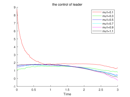
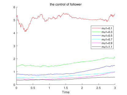
Refer to caption
(a) The impact of μ1subscript𝜇1\mu_{1} on leader’s advertising rate
Refer to caption
(b) The impact of μ1subscript𝜇1\mu_{1} on follower’s local promotion effort
Figure 5: The relationship between v1,v2subscript𝑣1subscript𝑣2v_{1},v_{2} and μ1subscript𝜇1\mu_{1}

In Figure 5, we study the quadratic cost coefficient μ1subscript𝜇1\mu_{1}’s effect on the promotion v1subscript𝑣1v_{1} and advertising effort v2subscript𝑣2v_{2}. First, in the left subfigure, we can see most lines hold a relatively steady and similar trend when the value of μ1subscript𝜇1\mu_{1} varies from 0.3 to 1.1, except for red line corresponding to μ1=0.1subscript𝜇10.1\mu_{1}=0.1. Although the red line show a strange tendency, we can give a reasonable explanation. For the common goal which is to increase sales revenue and decrease cost, in the case of μ1=0.1subscript𝜇10.1\mu_{1}=0.1, the cost coefficient of retailer’s local promotion effort is the smallest. The manufacturer knows it is benefit for the retailer to strengthen the advertising effort, which can guarantee the ideal sales revenue, so he choose to reduce the strength of advertising effort in a period of time, but hold a stable advertising rate in the later period of time because he have to control that the brand image is not too negatively affected by the retailer. In the right subfigure, it is evident that the lower the cost coefficient, the stronger the retailer’s promotion. Furthermore, the smallest cost coefficient stimulate the retailer’s promotion which is suppressed as the cost coefficient goes up. Finally, it drops to a lowest level that the retailer have to receive and keep unchanged.

We finally study the changes of x,x^,xˇ𝑥^𝑥ˇ𝑥x,\hat{x},\check{x} when μ1subscript𝜇1\mu_{1} takes these values in [0.1,0.3,0.5,0.7,0.9,1.1]0.10.30.50.70.91.1[0.1,0.3,0.5,0.7,0.9,1.1], that is, compared to the quadratic cost coefficient of the manufacturer, we concern the fluctuations of brand image itself, brand image observed by the retailer and that observed by the manufacturer, respectively, if the retailer’s cost weight increases or decreases.
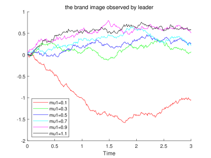
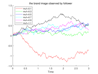
Refer to caption
(a) The impact of μ1subscript𝜇1\mu_{1} on xˇˇ𝑥\check{x}
Refer to caption
(b) The impact of μ1subscript𝜇1\mu_{1} on x^^𝑥\hat{x}
Refer to caption
(c) The impact of μ1subscript𝜇1\mu_{1} on x𝑥x
Figure 6: The relationship between xˇ,x^,xˇ𝑥^𝑥𝑥\check{x},\hat{x},x and μ1subscript𝜇1\mu_{1}

In Figure 6, except for the case of μ1=0.1subscript𝜇10.1\mu_{1}=0.1, the other cases all show that the brand image have a normal fluctuation influenced by the manufacturer’s advertising rate and the retailer’s local promotion, and present a positive effect on the brand image in general. But when μ1subscript𝜇1\mu_{1} becomes sufficiently small, which is a situation beyond the control, the retailer’s negative effect on the brand image will be magnified, which illustrate the tendency of red line in all three subfigures.

6 Concluding remarks

In this paper, we have studied an LQ partially observed Stackelberg differential game, different from the existing literatures [32], [37], where both the leader and the follower can only observe the state process through their own observation process. Different from [21], [22] and [57], for the technical need, the information available to the leader is less than that available to the follower. In order to obtain the necessary and sufficient conditions of the Stackelberg equilibrium point, we mainly utilize the state decomposition and backward separation techniques to solve the circular dependence between the observation process Y1(Y2)subscript𝑌1subscript𝑌2Y_{1}(Y_{2}) and control variable v1(v2v_{1}(v_{2}, respectively). First, the LQ partially observed optimal control problem of the follower is solved, and we get the state estimation feedback of optimal control via the FBSDFEs and one Riccati equation. Then, we introduce a new LQ partially observed optimal control problem of the leader where the state equation is not only driven by the tsubscript𝑡\mathcal{F}_{t}-standard Brownian motions W,W¯𝑊¯𝑊W,\bar{W}, but also by another tY1superscriptsubscript𝑡subscript𝑌1\mathcal{F}_{t}^{Y_{1}}-Brownian motion W~~𝑊\widetilde{W} (innovation process) which is not independent of W𝑊W or W¯¯𝑊\bar{W}, whose unique solvability can be obtained by a new combined idea. Meanwhile, a kind of fully-coupled FBSDE with filtering is studied as a by-product. Then we get the feedback representation form via an SDFE, a semi-martingale and three high-dimensional Riccati equations. We also study a special partially observed case and give the explicit expression of Stackelberg equilibrium points. Finally, we solve a dynamic cooperative advertising problem with asymmetric information and verify the effectiveness of proposed theoretical result by numerical simulation, moreover, we also discuss the relationship between the Stackelberg equilibrium points, state estimate and some practical parameters.

Possible extensions to the Stackelberg stochastic differential game with mixed leadership [2], [5], multiple followers [27], [37] and delayed systems [48], [49] promise to be interesting research topics. We will consider these challenging topics in our future work.

References

  • [1] T. Başar, G. J. Olsder, Dynamic Noncooperative Game Theory, 2nd Edition, SIAM, Philadelphia, 1998.
  • [2] T. Başar, A. Bensoussan, and S. P. Sethi, Differential games with mixed leadership: The open-loop solution. Appl. Math. Comput., 217(3), 972-979, 2010.
  • [3] A. Bensoussan, Stochastic Control of Partially Observable Systems, Cambridge University Press, 1992.
  • [4] A. Bensoussan, M. Viot, Optimal control of stochastic linear distributed parameter systems. SIAM J. Control Optim., 13(4), 904-926, 1975.
  • [5] A. Bensoussan, S. K. Chen, A. Chutani, S. P. Sethi, C. C. Siu, and S. C. P. Yam, Feedback Stackelberg-Nash equilibrium in mixed leadeship games with an application to cooperative advertising. SIAM J. Control Optim., 57(5), 3413-3444, 2019.
  • [6] A. Bensoussan, S. K. Chen, and S. P. Sethi, The maximum principle for global solutions of stochastic Stackelberg differential games. SIAM J. Control Optim., 53(4), 1956-1981, 2015.
  • [7] D. Castanon, M. Athans, On stochastic dynamic Stackelberg strategies. Automatica, 12(2), 177-183, 1976.
  • [8] L. Chen, Y. Shen, On a new paradigm of optimal reinsurance: A stochastic Stackelberg differential game between an insurer and a reinsurer. ASTIN Bulletin, 48(2), 905-960, 2018.
  • [9] J. Cvitanić, J. F. Zhang, Contract Theory in Continuous-Time Models, Springer-Verlag, Berlin, 2013.
  • [10] S. Davis, J. J. Inman, and L. McAlister, Promotion has a negative effect on brand evaluations-Or does it? Additional disconfirming evidence. J. Mark. Res., 29(1), 143-148, 1992.
  • [11] K. Du, Z. Wu, Linear-quadratic Stackelberg game for mean-field backward stochastic differential system and application. Math. Prob. Engin., 2019, Article ID 1798585, 17 pages.
  • [12] X. W. Feng, Y. Hu, and J. H. Huang, Backward Stackelberg differential game with constraints: a mixed terminal-perturbation and linear-quadratic approach, arXiv:2005.11872v1, May 2020.
  • [13] J. H. Huang, K. H. Si, and Z. Wu, Linear-quadratic mixed Stackelberg-Nash stochastic differential game with major-minor agents. Appl. Math. Opt., https://doi.org/10.1007/s00245-020-09713-z.
  • [14] J. H. Huang, G. C. Wang, and J. Xiong, A maximum principle for partial information backward stochastic control problems with applications. SIAM J. Control Optim., 48(4), 2106-2117, 2009.
  • [15] S. Jorgensen, S. P. Sigue, and G. Zaccour, Dynamic cooperative advertising in a channel. J. Retail., 76(1), 71-92, 2000.
  • [16] S. Jorgensen, S. Taboubi, and G. Zaccour, Cooperative advertising in a marketing channel. J. Optim. Theory Appl., 110(1), 145-158, 2001.
  • [17] S. Jorgensen, S. Taboubi, and G. Zaccour, Retail promotions with negative brand image effects: Is cooperation possible? Eur. J. Oper. Res., 150, 395-405, 2003.
  • [18] N. Li, Z. Y. Yu, Forward-backward stochastic differential equations and linear-quadratic generalized Stackelberg games. SIAM J. Control Optim., 56(6), 4148-4180, 2018.
  • [19] T. Li, S. P. Sethi, A review of dynamic Stackelberg game models. Discrete Contin. Dyn. Syst., Ser. B, 22(1), 125-159, 2017.
  • [20] X. J. Li, S. J. Tang, General necessary conditions for partially observed optimal stochastic controls. J. Appl. Probab., 32, 1118-1137, 1995.
  • [21] Z. P. Li, M. Y. Fu, Q. Q. Cai, and W. Meng, Leader-follower stochastic differential games under partial observation. In: Proc. 38th Chinese Control Conference, 1888-1892, Guangzhou, China, July 27-30, 2019.
  • [22] Z. P. Li, D. Marelli, M. Y. Fu, Q. Q. Cai, and W. Meng, Linear quadratic Gaussian Stackelberg game under asymmetric information patterns. Automatica, 125, 109406, 2021.
  • [23] A. E. B. Lim, X. Y. Zhou, Linear-quadratic control of backward stochastic differential equations. SIAM J. Control Optim., 40(2), 450-474, 2001.
  • [24] Y. N. Lin, X. S. Jiang, and W. H. Zhang, An open-loop Stackelberg strategy for the linear quadratic mean-field stochastic differential game. IEEE Trans. Autom. Control, 64(1), 97-110, 2019.
  • [25] R. S. Liptser, A. N. Shiryayev, Statistics of Random Processes, Springer-Verlag, New York, 1977.
  • [26] J. Moon, T. Başar, Linear quadratic mean field Stackelberg differential games. Automatica, 97, 200-213, 2018.
  • [27] H. Mukaidani, H. Xu, Stackelberg strategies for stochastic systems with multiple followers. Automatica, 53, 53-79, 2015.
  • [28] B. Øksendal, L. Sandal, and J. Ubøe, Stochastic Stackelberg equilibria with applications to time dependent newsvendor models. J. Econ. Dyna. &\& Control, 37(7), 1284-1299, 2013.
  • [29] P. Papatla, L. Krishnamurthi, Measuring the dynamic effects of promotions on brand choice. J. Mark. Res., 33(1), 20-35, 1996.
  • [30] S. G. Peng, Z. Wu, Fully coupled forward-backward stochastic differential equations and applications to optimal control. SIAM J. Control Optim., 37(3), 825-843, 1999.
  • [31] J. T. Shi, G. C. Wang, and J. Xiong, Leader-follower stochastic differential game with asymmetric information and applications. Automatica, 63, 60-73, 2016.
  • [32] J. T. Shi, G. C. Wang, and J. Xiong, Linear-quadratic stochastic Stackelberg differential game with asymmetric information. Sci. China Infor. Sci., 60, 092202:1-15, 2017.
  • [33] J. T. Shi, G. C. Wang, and J. Xiong, Stochastic linear quadratic Stackelberg differential game with overlapping information. ESAIM: Control, Optim. Calcu. Varia., 26, Article Number 83, 2020.
  • [34] J. T. Shi, Z. Wu, The maximum principle for partially observed optimal control of fully coupled forward-backward stochastic system. J. Optim. Theory Appl., 145(3), 543-578, 2010.
  • [35] H. von Stackelberg, The Theory of the Market Economy, Oxford University Press, London, 1952.
  • [36] S. J. Tang, The maximum principle for partially observed optimal control of stochastic differential equations. SIAM J. Control Optim. 36(5), 1596-1617, 1998.
  • [37] G. C. Wang, Y. Wang, and S. S. Zhang, An asymmetric information mean-field type linear-quadratic stochastic Stackelberg differential game with one leader and two followers. Optim. Control Appl. Meth., 41(4), 1034-1051, 2020.
  • [38] G. C. Wang, Z. Wu, Kalman-Bucy filtering equations of forward and backward stochastic systems and applications to recursive optimal control problems. J. Math. Anal. Appl., 342(2), 1280-1296, 2008.
  • [39] G. C. Wang, Z. Wu, The maximum principle for stochastic recursive optimal control problems under partial information. IEEE Trans. Autom. Control, 54(6), 1230-1242, 2009.
  • [40] G. C. Wang, Z. Wu, and J. Xiong, Maximum principles for forward-backward stochastic control systems with correlated state and observation noises. SIAM J. Control Optim., 51(1), 491-524, 2013.
  • [41] G. C. Wang, Z. Wu, and J. Xiong, A linear-quadratic optimal control problem of forward-backward stochastic differential equations with partial information. IEEE Trans. Autom. Control, 60(11), 2904-2916, 2015.
  • [42] G. C. Wang, Z. Wu, and J. Xiong, An Introduction to Optimal Control of FBSDE with Incomplete Information, Springer Briefs in Mathematics, Switzerland, 2018.
  • [43] Z. Wu, A maximum principle for partially observed optimal control of forward-backward stochastic control systems. Sci. China Infor. Sci., 53(11), 2205-2214, 2010.
  • [44] Z. Wu, Y. Zhuang, Linear-quadratic partially observed forward-backward stochastic differential games and its application in finance. Appl. Math. Comput., 321, 577-592, 2018.
  • [45] J. Xiong, An Introduction to Stochastic Filtering Theory, Oxford University Press, London, 2008.
  • [46] J. Xiong, X. Y. Zhou, Mean-variance portfolio selection under partial information. SIAM J. Control Optim., 46(1), 156-175, 2007.
  • [47] J. Xiong, S. Q. Zhang, and Y. Zhuang, A partially observed non-zero sum differential game of forward-backward stochastic differential equations and its application in finance. Math. Control Relat. Fields, 9(2), 257-276, 2019.
  • [48] J. J. Xu, J. T. Shi, and H. S. Zhang, A leader-follower stochastic linear quadratic differential game with time delay. Sci. China Infor. Sci., 61, 112202:1-13, 2018.
  • [49] J. J. Xu, H. S. Zhang, Sufficient and necessary open-loop Stackelberg strategy for two-player game with time delay. IEEE Trans. Cyber., 46(2), 438-449, 2016.
  • [50] W. S. Xu, Stochastic maximum principle for optimal control problem of forward and backward system. J. Aust. Math. Soc., Ser. B, 37, 172-185, 1995.
  • [51] J. M. Yong, A leader-follower stochastic linear quadratic differential games. SIAM J. Control Optim., 41(4), 1015-1041, 2002.
  • [52] J. M. Yong, Linear forward-backward stochastic differential equations. Appl. Math. Optim., 39(1), 93-119, 1999.
  • [53] J. M. Yong, X. Y. Zhou, Stochastic Controls: Hamiltonian Systems and HJB Equations, Springer-Verlag, New York, 1999.
  • [54] B. Yoo, N. Donthu, N. Lee, An examination of selected marketing mix elements and brand equity. J. Acad. Mark. Sci., 28(2), 195-211, 2000.
  • [55] Y. Y. Zheng, J. T. Shi, A Stackelberg game of backward stochastic differential equations with applications. Dyn. Games Appl., 10, 968-992, 2020.
  • [56] Y. Y. Zheng, J. T. Shi, A linear quadratic Stackelberg game of backward stochastic differential equations with partial information. In: Proc. 39th Chinese Control Conference, 966-971, Shenyang, China, July 27-29, 2020.
  • [57] Y. Y. Zheng, J. T. Shi, Stackelberg stochastic differential game with asymmetric noisy observations. To appear in Inter. J. Control. DOI: 10.1080/00207179.2021.1916078