Dynamic Algorithms for Online Multiple Testing

Ziyu Xu1,2 and Aaditya Ramdas1,2
Machine Learning Department1
Department of Statistics and Data Science2
Carnegie Mellon University
ziyux@cs.cmu.edu, aramdas@cmu.edu
Abstract

We derive new algorithms for online multiple testing that provably control false discovery exceedance (FDX) while achieving orders of magnitude more power than previous methods. This statistical advance is enabled by the development of new algorithmic ideas: earlier algorithms are more “static” while our new ones allow for the dynamical adjustment of testing levels based on the amount of wealth the algorithm has accumulated. We demonstrate that our algorithms achieve higher power in a variety of synthetic experiments. We also prove that SupLORD can provide error control for both FDR and FDX, and controls FDR at stopping times. Stopping times are particularly important as they permit the experimenter to end the experiment arbitrarily early while maintaining desired control of the FDR. SupLORD is the first non-trivial algorithm, to our knowledge, that can control FDR at stopping times in the online setting.

1 Introduction to Online Multiple Testing

Online multiple hypothesis testing has become an area of recent interest due to the massively increasing rate at which analysts are able to test hypotheses, both in the sciences and in the tech industry. This has been a result of the growth in computational resources for automating the generation and testing of new hypotheses (and collection of data to test them).

Online multiple testing is an abstraction of the scientific endeavor — the broad goal is to test a (potentially infinite) sequence of hypotheses H1,H2,subscript𝐻1subscript𝐻2H_{1},H_{2},\dots one by one over time. For example Hisubscript𝐻𝑖H_{i} could state that Alzheimer’s drug i𝑖i is no more effective than a placebo, and if we reject this hypothesis, we are effectively proclaiming a “discovery”. Some hypotheses are truly “null”, meaning that there really is no effect of interest, and the rest are “non-null”, but we do not know which are which, and we must use the data collected to identify as many non-null hypotheses as possible (making “true discoveries”), while not rejecting too many truly null hypotheses (avoid making “false discoveries”). Importantly, in the online setting, a decision to reject (or not reject) hypothesis Hksubscript𝐻𝑘H_{k} at time k𝑘k is irrevocable and cannot be altered at a future time.

It is important to note that the setup assumes that algorithm (or analyst) never finds out whether a hypothesis was correctly rejected or not. In other words, we do not know (until perhaps years later, after a lot of followup time and money has been invested) which of our proclaimed discoveries were true discoveries and which were false. Thus the false discovery proportion (FDPFDP\mathrm{FDP}), which is the ratio of false to total discoveries is an unobserved random variable, and we would like to make many discoveries (have high “power”) while keeping the FDPFDP\mathrm{FDP} small.

Previous algorithms for multiple testing have primarily focused on the false discovery rate (FDRFDR\mathrm{FDR}), which is the expectation of the FDPFDP\mathrm{FDP}. However, in practice, users may be more interested in a probabilistic bound of the tail of the FDPFDP\mathrm{FDP} as it offers a stricter guarantee about the distribution of the FDPFDP\mathrm{FDP}. Thus, we are interested in controlling the false discovery exceedance (FDXFDX\mathrm{FDX}) , which is the probability the FDPFDP\mathrm{FDP} exceeds a predefined threshold. To accomplish this, we first must describe how hypotheses are tested in the online multiple testing problem. As stated prior, we are testing a infinite sequence of hypotheses H1,H2,subscript𝐻1subscript𝐻2H_{1},H_{2},\dots, and each hypothesis is either null or non-null. For each hypothesis, we perform some type of experiment, analyze the data, and arrive at a summary statistic known as a “p-variable” that is supported only in [0,1]01[0,1]. Colloquially, p-variables are known as p-values, but we use the name “p-variable” to emphasize the fact that p-variables are random variables, and not a probability value. We use “p-value” to denote the specific value a p-variable is sampled at. Typically, p-variables are the result of making certain sampling assumptions about the data, and deriving some type of statistic with a known distribution from the data — an excellent reference on how these statistics are derived is chapter 10 in Wasserman (2004). Hence, Pksubscript𝑃𝑘P_{k} is the p-variable whose distribution is based on the data drawn under hypothesis Hksubscript𝐻𝑘H_{k}, and pksubscript𝑝𝑘p_{k} will be the corresponding p-value to Pksubscript𝑃𝑘P_{k}. If Hksubscript𝐻𝑘H_{k} is null, then the the distribution of Pksubscript𝑃𝑘P_{k} must be stochastically larger than uniform. We will formalize this notion later, but the key message here is that we essentially know what the distribution of the p-variable under the null hypothesis is.

As a result, an online multiple testing algorithm is primarily concerned with the stream of p-values p1,p2,subscript𝑝1subscript𝑝2p_{1},p_{2},\dots, which correspond to the sequence of hypotheses being tested. For each hypothesis Hksubscript𝐻𝑘H_{k}, the algorithm must output an alpha value, αksubscript𝛼𝑘\alpha_{k}, in [0,1]01[0,1], based solely on the previous p-values it has received i.e. p1,,pk1subscript𝑝1subscript𝑝𝑘1p_{1},\dots,p_{k-1}. Critically, it must output this alpha value before receiving the next p-value pksubscript𝑝𝑘p_{k}. Hksubscript𝐻𝑘H_{k} is then rejected if pksubscript𝑝𝑘p_{k} is less than or equal to αksubscript𝛼𝑘\alpha_{k}. We denote the set of rejected hypotheses up to the k𝑘kth hypothesis as k{1,,k}subscript𝑘1𝑘\mathcal{R}_{k}\subseteq\left\{1,\dots,k\right\}. The set of null hypothesis is denoted as 0subscript0\mathcal{H}_{0}\subseteq\mathbb{N}. We let the set of null rejections (i.e. false discoveries) in the first be k𝑘k hypotheses be denoted as Vk=0ksubscript𝑉𝑘subscript0subscript𝑘V_{k}=\mathcal{H}_{0}\cap\mathcal{R}_{k}. Thus, the FDPFDP\mathrm{FDP} of ksubscript𝑘\mathcal{R}_{k} is defined as follows:

FDP(k)FDPsubscript𝑘\displaystyle\mathrm{FDP}(\mathcal{R}_{k}) |Vk||k|1.absentsubscript𝑉𝑘subscript𝑘1\displaystyle~{}\equiv~{}\frac{\left|V_{k}\right|}{\left|\mathcal{R}_{k}\right|\lor 1}.

Define the (simultaneous, or time-uniform) FDXKsubscriptFDX𝐾\mathrm{FDX}_{K} as the probability that the FDPFDP\mathrm{FDP} ever exceeds a threshold ϵ(0,1)superscriptitalic-ϵ01\epsilon^{*}\in(0,1) after time K𝐾K:

FDXKϵ𝐏𝐫(supkKFDP(k)ϵ).superscriptsubscriptFDX𝐾superscriptitalic-ϵ𝐏𝐫𝑘𝐾supremumFDPsubscript𝑘superscriptitalic-ϵ\displaystyle\mathrm{FDX}_{K}^{\epsilon^{*}}~{}\equiv~{}\mathbf{Pr}\left(\underset{k\geq K}{\sup}\ \mathrm{FDP}(\mathcal{R}_{k})\geq\epsilon^{*}\right).

The FDRFDR\mathrm{FDR} in the online setting is a pointwise guarantee for each hypothesis i.e. it is the largest expected FDPFDP\mathrm{FDP} for any fixed time after K𝐾K:

FDR(k)FDRsubscript𝑘\displaystyle\mathrm{FDR}(\mathcal{R}_{k}) 𝔼[FDP(k)],FDRKsupkKFDR(k).formulae-sequenceabsent𝔼delimited-[]FDPsubscript𝑘subscriptFDR𝐾𝑘𝐾supremumFDRsubscript𝑘\displaystyle~{}\equiv~{}\mathbb{E}\left[\mathrm{FDP}(\mathcal{R}_{k})\right],\qquad\mathrm{FDR}_{K}~{}\equiv~{}\underset{k\geq K}{\sup}\ \mathrm{FDR}(\mathcal{R}_{k}).

(In prior work FDRFDR\mathrm{FDR} and FDXFDX\mathrm{FDX} have been defined with K=1𝐾1K=1.) We also provide the first algorithm that controls a related time-uniform error metric, which is the expectation of the largest FDPFDP\mathrm{FDP}:

SupFDRK𝔼[supkKFDP(k)].subscriptSupFDR𝐾𝔼delimited-[]𝑘𝐾supremumFDPsubscript𝑘\displaystyle\mathrm{SupFDR}_{K}\equiv\mathbb{E}\left[\underset{k\geq K}{\sup}\ \mathrm{FDP}(\mathcal{R}_{k})\right].

Any algorithm that controls SupFDR1subscriptSupFDR1\mathrm{SupFDR}_{1} at a level \ell will also control FDR1subscriptFDR1\mathrm{FDR}_{1} at \ell as well, since SupFDRSupFDR\mathrm{SupFDR} is strictly larger than FDRFDR\mathrm{FDR}. One central difference is that FDR1subscriptFDR1\mathrm{FDR}_{1}\leq\ell does not yield a guarantee at a data-dependent stopping time τ𝜏\tau, but SupFDR1subscriptSupFDR1\mathrm{SupFDR}_{1}\leq\ell does imply that FDR(τ)FDRsubscript𝜏\mathrm{FDR}(\mathcal{R}_{\tau})\leq\ell. This yields the first FDR guarantee at stopping times in the literature. In past work “anytime FDR control” really held at any fixed time (when the time is specified in advance), but controlling SupFDRSupFDR\mathrm{SupFDR} truly makes the aforementioned phrase actionable in the online setting, since it is a simultaneous guarantee over all time. We expand on the relationship between these two error metrics in Section 1.2. We aim to maximize power, which is the expected proportion of non-null hypotheses that are rejected:

Power(k)𝔼[|k0c||0c|].Powersubscript𝑘𝔼delimited-[]subscript𝑘superscriptsubscript0𝑐superscriptsubscript0𝑐\displaystyle\mathrm{Power}(\mathcal{R}_{k})~{}\equiv~{}\mathbb{E}\left[\frac{\left|\mathcal{R}_{k}\cap\mathcal{H}_{0}^{c}\right|}{\left|\mathcal{H}_{0}^{c}\right|}\right].

Thus, the problem of online multiple testing is to design an algorithm that rejects as as many non-null hypotheses as possible while not rejecting null hypotheses to a degree that is sufficient to satisfy the desired level of control on an error metric (e.g. FDR, FDX, SupFDRSupFDR\mathrm{SupFDR}).

We do not make guarantees about the optimality of power. This is because we do not have any information about the alternate hypothesis and make no assumptions about the distribution and frequency of non-null hypotheses. However, we can assert that the error metric is provably controlled, since it is only dependent on null hypotheses.

The LORDLORD\mathrm{LORD} algorithm, introduced by Javanmard and Montanari (2018), is an online multiple testing algorithm that provably controls the FDRFDR\mathrm{FDR} at level \ell (i.e.  guarantees FDRFDR\mathrm{FDR} will be less than \ell). We will refer to Javanmard and Montanari (2018) as JM in the sequel. JM show that LORDLORD\mathrm{LORD}, with additional constraints, controls FDXFDX\mathrm{FDX}. We will refer to this version of LORDLORD\mathrm{LORD} as LORDFDXLORDFDX\mathrm{LORD}\mathrm{FDX}. LORDFDXLORDFDX\mathrm{LORD}\mathrm{FDX} is the only existing rule that controls FDXFDX\mathrm{FDX} at a set level to the best of our knowledge. We determine, through experiments, that LORDFDXLORDFDX\mathrm{LORD}\mathrm{FDX} is extremely conservative and we design an algorithm that significantly improves power while controlling FDXFDX\mathrm{FDX} at the same level.

Our proofs employ the post-hoc probabilistic bounds on the FDPFDP\mathrm{FDP} developed by Katsevich and Ramdas (2020), which we refer to as KR henceforth. KR do not propose an algorithm for guaranteeing a certain level of FDXFDX\mathrm{FDX} control, but rather formulate an algorithm-agnostic bound based on any sequence of alpha values {αi}iksubscriptsubscript𝛼𝑖𝑖𝑘\{\alpha_{i}\}_{i\leq k} and rejection sets ksubscript𝑘\mathcal{R}_{k}, in order to form a time-uniform confidence interval for the FDPFDP\mathrm{FDP}. We view our work as an algorithmic mechanization of these bounds such that the FDXFDX\mathrm{FDX} can be controlled by the practitioner in a premeditated fashion.

1.1 Notation and P-Variable Assumptions

Abbreviations.

We abbreviate a few works that will be referenced often. As mentioned in the prequel, JM refers to Javanmard and Montanari (2018) and KR refers to Katsevich and Ramdas (2020). FS refers to Foster and Stine (2008), which is the original work in this area.

Notation.

Recall that Pksubscript𝑃𝑘P_{k} is the k𝑘kth p-variable and αksubscript𝛼𝑘\alpha_{k} is the k𝑘kth alpha value. Let Rk=𝐈{Pkαk}subscript𝑅𝑘𝐈subscript𝑃𝑘subscript𝛼𝑘R_{k}=\mathbf{I}\left\{P_{k}\leq\alpha_{k}\right\} indicate whether the k𝑘kth hypothesis is rejected. Generally, script variables such as ,,\mathcal{H},\mathcal{R},\mathcal{F} are sets. Capital letters, such as R,V,W,P𝑅𝑉𝑊𝑃R,V,W,P are random variables. Greek letters, such as α,β,γ,δ,ϵ𝛼𝛽𝛾𝛿italic-ϵ\alpha,\beta,\gamma,\delta,\epsilon, represent user selected parameters for the algorithm. We collect the “past rejection information” into a filtration:

kσ({Ri}ik),subscript𝑘𝜎subscriptsubscript𝑅𝑖𝑖𝑘\displaystyle\mathcal{F}_{k}~{}\equiv~{}\sigma(\left\{R_{i}\right\}_{i\leq k}), (1)

with 0subscript0\mathcal{F}_{0} being the trivial σ𝜎\sigma-algebra. Note that {αk}ksubscriptsubscript𝛼𝑘𝑘\{\alpha_{k}\}_{k\in\mathbb{N}} is predictable with respect to {k}ksubscriptsubscript𝑘𝑘\{\mathcal{F}_{k}\}_{k\in\mathbb{N}} meaning that αksubscript𝛼𝑘\alpha_{k} is k1subscript𝑘1\mathcal{F}_{k-1}-measurable.

P-variable assumptions.

In classical hypothesis testing, a p-variable is a random variable whose distribution is stochastically larger than uniform under the null, meaning that if the null hypothesis is true, we would have 𝐏𝐫(Ps)s𝐏𝐫𝑃𝑠𝑠\mathbf{Pr}\left(P\leq s\right)\leq s for all s[0,1]𝑠01s\in[0,1]. For the online setting, the weakest possible assumption one could make is that conditional on the past, the p-variables still satisfy such a condition. This is usually formalized (by FS, Ramdas et al. 2017, and KR, for example), by the following conditional superuniformity assumption about null p-variables:

𝐏𝐫(Pk+1sk)s for k0,s[0,1].formulae-sequence𝐏𝐫subscript𝑃𝑘1conditional𝑠subscript𝑘𝑠 for 𝑘subscript0𝑠01\displaystyle\mathbf{Pr}\left(P_{k+1}\leq s\mid\mathcal{F}_{k}\right)\leq s\text{ for }k\in\mathcal{H}_{0},\ s\in[0,1]. (2)

Note that the above assumption is weaker than assuming that the p-variables are independently, superuniformly distributed under the null hypothesis:

𝐏𝐫(Pks)s for k0,s[0,1] and {Pk}k0 are jointly independent,formulae-sequence𝐏𝐫subscript𝑃𝑘𝑠𝑠 for 𝑘subscript0𝑠01 and subscriptsubscript𝑃𝑘𝑘subscript0 are jointly independent\displaystyle\mathbf{Pr}\left(P_{k}\leq s\right)\leq s\text{ for }k\in\mathcal{H}_{0},\ s\in[0,1]\text{ and }\{P_{k}\}_{k\in\mathcal{H}_{0}}\text{ are jointly independent}, (3)

which is also commonly made in the online FDR literature (in JM, for example). For the rest of the paper, we make no further assumptions on the relationship between on the hypotheses, H1,H2,subscript𝐻1subscript𝐻2H_{1},H_{2},\dots other than (2). We include assumption (3) because it implies (2) and has been used to prove error control in prior work e.g. LORDLORD\mathrm{LORD} requires this assumption for FDRFDR\mathrm{FDR} control. Hence, the online multiple testing is a relatively assumption-light framework that can be adapted to many practical settings. Lastly, we define trsubscript𝑡𝑟t_{r} to be the time step when the r𝑟rth rejection is made, where r𝑟r is a positive integer.

1.2 Summary of Contributions
Refer to caption
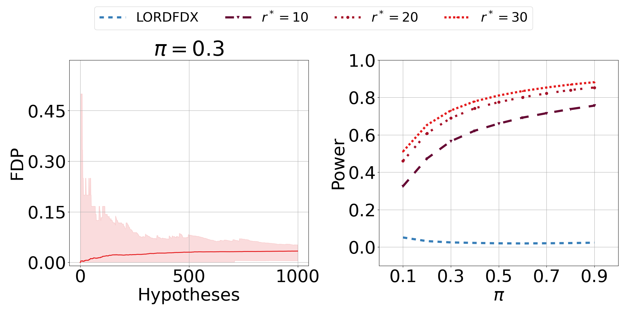
Figure 1: The right plot is the power of SupLORDSupLORD\mathrm{SupLORD}, for different delays in rejections, rsuperscript𝑟r^{*}, vs. LORDFDXLORDFDX\mathrm{LORD}\mathrm{FDX} from JM. The left plot is the average FDPFDP\mathrm{FDP} of SupLORDSupLORD\mathrm{SupLORD} with r=30superscript𝑟30r^{*}=30 across hypotheses tested for non-null likelihoods π{0.1,0.3}𝜋0.10.3\pi\in\{0.1,0.3\}. All algorithms control FDXFDX\mathrm{FDX} for ϵ=0.15superscriptitalic-ϵ0.15\epsilon^{*}=0.15 at a level of δ=0.05superscript𝛿0.05\delta^{*}=0.05. Experiment details are in Section 3.2. The shaded area is a 1δ1superscript𝛿1-\delta^{*} confidence band for the FDPFDP\mathrm{FDP} — it is smaller than ϵsuperscriptitalic-ϵ\epsilon^{*} for the majority of hypotheses. This shows FDXFDX\mathrm{FDX} control at ϵsuperscriptitalic-ϵ\epsilon^{*} holds for a substantial portion of the hypotheses. Also, the power of SupLORDSupLORD\mathrm{SupLORD} increases with rsuperscript𝑟r^{*}. Thus, SupLORDSupLORD\mathrm{SupLORD} has significant FDXFDX\mathrm{FDX} control and more power than LORDFDXLORDFDX\mathrm{LORD}\mathrm{FDX} (by JM).

Delayed FDX control.

We provide a formula for SupLORDSupLORD\mathrm{SupLORD}, which controls FDXFDX\mathrm{FDX} at a set level, and has more power than LORDFDXLORDFDX\mathrm{LORD}\mathrm{FDX} (by JM). In fact, we observe empirically that LORDFDXLORDFDX\mathrm{LORD}\mathrm{FDX} rejects only a few hypotheses before becoming unable to reject any more hypotheses, and performs no better than the baseline approach we discuss in Section 2.1. We prove SupLORDSupLORD\mathrm{SupLORD} controls FDXFDX\mathrm{FDX} by using a time-uniform confidence interval introduced in KR on the FDPFDP\mathrm{FDP}. A novel feature of our algorithm is that we may choose the number of rejections after which we begin controlling FDXFDX\mathrm{FDX} in exchange for more power. Practically, users often test a large number of hypotheses, and make many discoveries. Thus, the small number of rejections with no FDXFDX\mathrm{FDX} control is an insignificant fraction of the experiment. The right plot in Figure 1 shows that having the FDXFDX\mathrm{FDX} bound apply after only 10 rejections is sufficient for a noticeable increase in power over LORDFDXLORDFDX\mathrm{LORD}\mathrm{FDX}. The left plot indicates that the FDXFDX\mathrm{FDX} is still controlled for a substantial proportion of the hypotheses, despite delaying control for 30 rejections. Consequently, we show through experimental results111Code for the figures and experiments in this paper can be found at https://github.com/neilzxu/suplord. that by affording this flexibility to our algorithm, it can improve power with no practical deficit.

Dynamic scheduling.

Many multiple testing algorithms, including SupLORDSupLORD\mathrm{SupLORD}, are based upon a notion of generalized alpha-investing introduced by Aharoni and Rosset (2014) which maintains a nonnegative value known as wealth. Wealth quantifies the error budget of the algorithm, and is an upper bound on the size of the next alpha value. For our error metrics of interest, an algorithm gains wealth by making rejections. We discuss and formalize the role of wealth in Section 2. Deciding how to allocate an algorithm’s wealth to alpha values is a key challenge of designing online multiple testing algorithms. We devise a method for formulating alpha values that dynamically chooses larger alpha values when wealth is large. Through experiments, we demonstrate that SupLORDSupLORD\mathrm{SupLORD} with dynamic scheduling outperforms spending schedules introduced in JM, and fully utilizes its wealth and increases its power as a result.

Theoretical improvements in FDRFDR\mathrm{FDR} control.

The SupLORDSupLORD\mathrm{SupLORD} algorithm is able to control not only FDXFDX\mathrm{FDX}, but also FDRFDR\mathrm{FDR} and SupFDRSupFDR\mathrm{SupFDR} at a set level of control. Table 1 illustrates the difference in assumptions and error control guarantees between SupLORDSupLORD\mathrm{SupLORD} and existing methods. Without imposing more restrictive independence assumptions and reducing the regime of control to fixed times, previous algorithms (FS, JM, Ramdas et al. 2017, 2018; Tian and Ramdas 2019) could only control a modified FDRFDR\mathrm{FDR}:

mFDR(k)mFDRsubscript𝑘\displaystyle\mathrm{mFDR}(\mathcal{R}_{k}) 𝔼[|Vk|]𝔼[|k|1].absent𝔼delimited-[]subscript𝑉𝑘𝔼delimited-[]subscript𝑘1\displaystyle~{}\equiv~{}\frac{\mathbb{E}\left[|V_{k}|\right]}{\mathbb{E}\left[\left|\mathcal{R}_{k}\right|\vee 1\right]}. (4)

By controlling SupFDRSupFDR\mathrm{SupFDR}, SupLORDSupLORD\mathrm{SupLORD} controls FDRFDR\mathrm{FDR} under the same guarantees and assumptions as previous algorithms that controlled mFDRmFDR\mathrm{mFDR}. Specifically, SupLORDSupLORD\mathrm{SupLORD} offers the following theoretical improvements for control of FDRFDR\mathrm{FDR}:

  1. 1.

    Control at stopping times. Stopping times are random times that are a function of past events. Previous results have only controlled FDRFDR\mathrm{FDR} at fixed times. Consequently, this enables to the user to stop SupLORDSupLORD\mathrm{SupLORD} prematurely, and still maintain valid FDRFDR\mathrm{FDR} bounds.

  2. 2.

    Non-monotonicity. The spending schedule in prior work required αksubscript𝛼𝑘\alpha_{k} to be monotone, that is:

    αk is coordinatewise nondecreasing w.r.t. past rejections R1,,Rk1for all k1.subscript𝛼𝑘 is coordinatewise nondecreasing w.r.t. past rejections subscript𝑅1subscript𝑅𝑘1for all 𝑘1\displaystyle\alpha_{k}\text{ is coordinatewise nondecreasing w.r.t. past rejections }R_{1},\dots,R_{k-1}\ \text{for all }k\geq 1. (5)

    However, SupLORDSupLORD\mathrm{SupLORD} has a provable FDRFDR\mathrm{FDR} guarantee without this constraint on its spending schedule due to using techniques from KR. Thus, when using non-monotonic schedules such as dynamic scheduling, SupLORDSupLORD\mathrm{SupLORD} maintains a provable FDRFDR\mathrm{FDR} guarantee.

  3. 3.

    Non-independence. Prior algorithms require independent p-values to have FDRFDR\mathrm{FDR} control. SupLORDSupLORD\mathrm{SupLORD} only requires a natural, weaker, baseline assumption we formalize in (2). This assumption is required to prove any known guarantee for online multiple testing algorithms.

Table 1: Comparison of the error metrics controlled under different assumptions of online multiple testing algorithms discussed in Section 1.2. Note that assumption (3) implies assumption (2), and hence any guarantees achieved under (2) are also achieved under (3). To achieve FDRFDR\mathrm{FDR} control, all algorithms except SupLORDSupLORD\mathrm{SupLORD} require both independent superuniform p-variables, and monotone spending schedules — SupLORDSupLORD\mathrm{SupLORD} can offer FDRFDR\mathrm{FDR} guarantees under only conditional superuniformity (2). In addition, SupLORDSupLORD\mathrm{SupLORD} is the only algorithm that offers control of FDRFDR\mathrm{FDR} at stopping times and FDXFDX\mathrm{FDX} control without alpha-death, as LORDFDXLORDFDX\mathrm{LORD}\mathrm{FDX} suffers from alpha-death.
Method Guarantees
LORDLORD\mathrm{LORD}, SAFFRONSAFFRON\mathrm{SAFFRON}, ADDISADDIS\mathrm{ADDIS} If p-variables satisfy
(JM, Ramdas et al. 2017 If p-variables satisfy independence,
Ramdas et al. 2018, conditional superuniformity (2): superuniformity (3),
Tian and Ramdas 2019)   mFDRmFDR\mathrm{mFDR} at stopping times and monotone spending (5):
  FDRFDR\mathrm{FDR} at fixed times
  mFDRmFDR\mathrm{mFDR} at stopping times
SupLORDSupLORD\mathrm{SupLORD} If p-variables satisfy conditional superuniformity (2):
  FDRFDR\mathrm{FDR} at stopping times (Corollary 2)
  FDXFDX\mathrm{FDX} w/o alpha-death (Theorem 1)
  mFDRmFDR\mathrm{mFDR} at stopping times (Theorem 6)

2 Generalized Alpha-Investing (GAI)

One of the key paradigms in online hypothesis testing is notion of alpha-investing that was first introduced by Foster and Stine (2008), and expanded upon in later works (Aharoni and Rosset, 2014; Ramdas et al., 2017). Our primary error metric of interest in this section will be FDRFDR\mathrm{FDR}, since prior algorithms, including LORDLORD\mathrm{LORD}, have focused on controlling FDRFDR\mathrm{FDR}. However, this paradigm is generalizable to any of the error metrics we consider in this paper. In particular, we will see how we use this idea to derive our new algorithm, SupLORDSupLORD\mathrm{SupLORD}, in Section 3.

2.1 Alpha-Spending and Alpha-Death

To elucidate alpha-investing, we first discuss the notion of alpha-spending, which is an Bonferroni correction. We control the FDR (indeed the familywise error rate, a more stringent criterion) by ensuring that the following constraint is satisfied at every k𝑘k:

i=1kαk.superscriptsubscript𝑖1𝑘subscript𝛼𝑘\displaystyle\sum_{i=1}^{k}\alpha_{k}\leq\ell. (6)

In condition (6), we can view \ell as our error budget, or wealth, since the sum of all alpha values adds up to \ell. Thus, we can imagine this as starting out with wealth of \ell, and spending no more than our current wealth on the current alpha value for each hypothesis. This method for choosing alpha values is known as alpha-spending. We can explicitly define the wealth at time k𝑘k for alpha-spending to be:

W(k)i=1kαi.𝑊𝑘superscriptsubscript𝑖1𝑘subscript𝛼𝑖\displaystyle W(k)~{}\equiv~{}\ell-\sum_{i=1}^{k}\alpha_{i}. (7)

Definition (7) indicates that wealth is monotonically decreasing when alpha-spending. As more hypotheses are tested, the alpha values will shrink towards zero. Thus, the algorithm will fail to reject nearly every future hypothesis after enough hypotheses are tested. Ramdas et al. (2017) term the shrinkage or disappearance of alpha values and consequent failure to reject hypotheses after a point in time as alpha-death. Alpha-spending suffers from alpha-death because the bound is extremely conservative — Bonferroni controls the probability of making even a single false rejection to be at level \ell as opposed to simply controlling the FDRFDR\mathrm{FDR} to be at \ell.

2.2 Generalized Alpha-Investing Algorithms

An alpha-investing example: LORDLORD\mathrm{LORD}.

To avoid alpha-death, we can choose a less conservative bound than Bonferroni while maintaining FDRFDR\mathrm{FDR} control. Ramdas et al. (2017) provide an estimator that upper bounds the FDRFDR\mathrm{FDR}:

FDP^LORD(k)=i=1kαi|k|1.subscript^FDPLORDsubscript𝑘superscriptsubscript𝑖1𝑘subscript𝛼𝑖subscript𝑘1\displaystyle\widehat{\mathrm{FDP}}_{\mathrm{LORD}}(\mathcal{R}_{k})=\frac{\sum_{i=1}^{k}\alpha_{i}}{\left|\mathcal{R}_{k}\right|\vee 1}. (8)

Notably, this is also the estimator that LORDLORD\mathrm{LORD} uses to control FDRFDR\mathrm{FDR}. Thus, we simply need to control FDP^LORDsubscript^FDPLORD\widehat{\mathrm{FDP}}_{\mathrm{LORD}} at level \ell, for the FDRFDR\mathrm{FDR} to be controlled at the same level. Hence, we get a different wealth formulation than in the alpha-spending case:

W(k)(|k|1)i=1kαi.𝑊𝑘subscript𝑘1superscriptsubscript𝑖1𝑘subscript𝛼𝑖\displaystyle W(k)~{}\equiv~{}\ell(|\mathcal{R}_{k}|\vee 1)-\sum_{i=1}^{k}\alpha_{i}. (9)

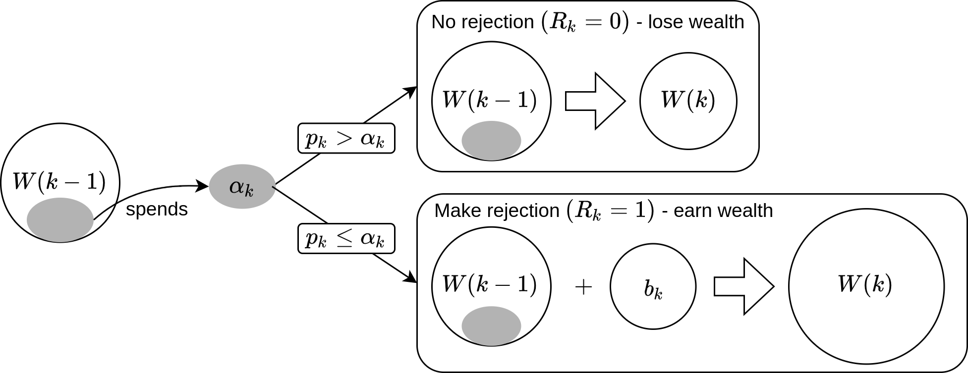
The key difference between this formulation and alpha-spending is that wealth can be earned. Thus, alpha-death is avoided since αisubscript𝛼𝑖\alpha_{i} need not shrink to zero. We obtain a reward of \ell each time the algorithm makes a rejection222In this formulation, the initial wealth is \ell and no wealth is gained from the first rejection, but this can be easily amended so that the sum of the initial wealth and first reward equals \ell using any other split. i.e. increases the cardinality of ksubscript𝑘\mathcal{R}_{k}. The wealth reward follows from (8) — when more hypotheses are rejected, the denominator in (8) increases, which allows for a larger numerator while maintaining the same FDP^LORDsubscript^FDPLORD\widehat{\mathrm{FDP}}_{\mathrm{LORD}} value. Thus, an algorithm may carefully “invest” its wealth on alpha values in a way that maximizes the number of rejections.

Generalized alpha-investing (GAI).

GAI algorithms have the following wealth update:

W(k)𝑊𝑘\displaystyle W(k) β0+i=1kβiRii=1kαi,absentsubscript𝛽0superscriptsubscript𝑖1𝑘subscript𝛽𝑖subscript𝑅𝑖superscriptsubscript𝑖1𝑘subscript𝛼𝑖\displaystyle~{}\equiv~{}\beta_{0}+\sum_{i=1}^{k}\beta_{i}R_{i}-\sum_{i=1}^{k}\alpha_{i}, (10)

where {βi}i{0}subscriptsubscript𝛽𝑖𝑖0\{\beta_{i}\}_{i\in\mathbb{N}\cup\{0\}} is the boost sequence and is nonnegative. βisubscript𝛽𝑖\beta_{i} is the boost in wealth that is earned from the algorithm making the rejection on the i𝑖ith hypothesis. Similar to alpha values, we require {βk}ksubscriptsubscript𝛽𝑘𝑘\{\beta_{k}\}_{k\in\mathbb{N}} to be predictable with respect to {k}ksubscriptsubscript𝑘𝑘\{\mathcal{F}_{k}\}_{k\in\mathbb{N}} and β0subscript𝛽0\beta_{0} to be a constant. We can recover (7) by setting βi=0subscript𝛽𝑖0\beta_{i}=0, and we can recover (9) by setting βi=subscript𝛽𝑖\beta_{i}=\ell. The key invariant that all alpha-investing algorithms maintain is the following:

αkW(k1).subscript𝛼𝑘𝑊𝑘1\displaystyle\alpha_{k}\leq W(k-1). (11)

Thus, selection of alpha values respects this notion of wealth and ensures it is always nonnegative.
Refer to caption
Figure 2: Diagram of the alpha-investing paradigm. The algorithm spends wealth at each hypothesis k𝑘k and earns wealth if it makes a rejection, and loses αksubscript𝛼𝑘\alpha_{k} wealth if it does not.

Spending schedule.

JM also proposed two methods of choosing alpha values (i.e. spending schedules) based on wealth. Let {γi}isubscriptsubscript𝛾𝑖𝑖\{\gamma_{i}\}_{i\in\mathbb{N}} be a spending sequence that has the following properties:

γi0 for all isubscript𝛾𝑖0 for all 𝑖\displaystyle\gamma_{i}\geq 0\text{ for all }i\in\mathbb{N} (12a)
i=1γi=1.superscriptsubscript𝑖1subscript𝛾𝑖1\displaystyle\sum\limits_{i=1}^{\infty}\gamma_{i}=1. (12b)

JM propose the following spending schedules:

αk={γkβ0+j=1|k1|γktjβtjsteadyγkt|k1|W(t|k1|)aggressive.subscript𝛼𝑘casessubscript𝛾𝑘subscript𝛽0superscriptsubscript𝑗1subscript𝑘1subscript𝛾𝑘subscript𝑡𝑗subscript𝛽subscript𝑡𝑗steadysubscript𝛾𝑘subscript𝑡subscript𝑘1𝑊subscript𝑡subscript𝑘1aggressive\displaystyle\alpha_{k}=\begin{cases}\gamma_{k}\beta_{0}+\sum\limits_{j=1}^{\left|\mathcal{R}_{k-1}\right|}\gamma_{k-t_{j}}\beta_{t_{j}}&\textsc{steady}\\ \gamma_{k-t_{|\mathcal{R}_{k-1}|}}W(t_{|\mathcal{R}_{k-1}|})&\textsc{aggressive}.\end{cases} (13)

While both are valid spending schedules in the sense that neither would violate condition (11), only steady can be used to provide provable FDRFDR\mathrm{FDR} control in LORDLORD\mathrm{LORD}, since steady is the only monotone rule (5). Intuitively, this means that when more rejections are made, a monotone spending schedule should output larger alpha values at all future time steps than it would if fewer rejections were made. JM show that steady satisfies monotonicity while aggressive does not. Hence, aggressive does not provide any FDRFDR\mathrm{FDR} guarantees when used with LORDLORD\mathrm{LORD}. In Section 5, we will discuss how SupLORDSupLORD\mathrm{SupLORD} can maintain FDRFDR\mathrm{FDR} control even when using non-monotone spending schedules.

For the spending sequence, a default choice is to set γilog(i2)iexp(logi)proportional-tosubscript𝛾𝑖𝑖2𝑖𝑖\gamma_{i}\propto\frac{\log(i\vee 2)}{i\exp(\sqrt{\log i})}, which is motivated by optimizing a lower bound for the power of LORDLORD\mathrm{LORD} in the Gaussian setting in JM.

3 SupLORDSupLORD\mathrm{SupLORD}: Delayed FDXFDX\mathrm{FDX} Control

We propose a new alpha-investing algorithm, SupLORDSupLORD\mathrm{SupLORD}, which provides control over the FDXFDX\mathrm{FDX}. SupLORDSupLORD\mathrm{SupLORD} requires the user to specify rsuperscript𝑟r^{*}, a threshold of rejections after which the error control begins to apply, ϵsuperscriptitalic-ϵ\epsilon^{*}, the upper bound on the FDPFDP\mathrm{FDP}, and δsuperscript𝛿\delta^{*}, the probability at which the FDPFDP\mathrm{FDP} exceeds ϵsuperscriptitalic-ϵ\epsilon^{*} at any time step after making rsuperscript𝑟r^{*} rejections. We derive this algorithm from a new estimator, FDP¯¯FDP\overline{\mathrm{FDP}}, that gives probabilistic, time-uniform control over the FDPFDP\mathrm{FDP}. Notably, SupLORDSupLORD\mathrm{SupLORD} requires no assumptions about relationships between hypotheses tested except for condition (2) on p-variables of null hypotheses.

3.1 Deriving the Boost Sequence

To prepare for the FDP¯¯FDP\overline{\mathrm{FDP}}, define the following quantities, respectively:

V^(k)^𝑉subscript𝑘\displaystyle\widehat{V}(\mathcal{R}_{k}) i=1kαi,absentsuperscriptsubscript𝑖1𝑘subscript𝛼𝑖\displaystyle~{}\equiv~{}\sum\limits_{i=1}^{k}\alpha_{i},
FDP^SupLORD(k)subscript^FDPSupLORDsubscript𝑘\displaystyle\widehat{\mathrm{FDP}}_{\mathrm{SupLORD}}(\mathcal{R}_{k}) V^(k)+1|k|.absent^𝑉subscript𝑘1subscript𝑘\displaystyle~{}\equiv~{}\frac{\widehat{V}(\mathcal{R}_{k})+1}{\left|\mathcal{R}_{k}\right|}.

Now, for any δ(0,1)𝛿01\delta\in(0,1), define

log¯(1δ)¯1𝛿\displaystyle{\overline{\log}}{\left(\frac{1}{\delta}\right)} log(1δ)log(1+log(1δ)).absent1𝛿11𝛿\displaystyle~{}\equiv~{}\frac{\log(\frac{1}{\delta})}{\log\left(1+\log(\frac{1}{\delta})\right)}.

Hence our estimator of interest is defined as follows:

FDP¯(k)¯FDPsubscript𝑘\displaystyle\overline{\mathrm{FDP}}(\mathcal{R}_{k}) log¯(1δ)FDP^(k).absent¯1superscript𝛿^FDPsubscript𝑘\displaystyle~{}\equiv~{}{\overline{\log}}{\left(\frac{1}{\delta^{*}}\right)}\cdot\widehat{\mathrm{FDP}}(\mathcal{R}_{k}).
Fact 1 (Theorem 4 from KR).

Let {αk}ksubscriptsubscript𝛼𝑘𝑘\{\alpha_{k}\}_{k\in\mathbb{N}} be any sequence of alpha values predictable with respect to filtration ksubscript𝑘\mathcal{F}_{k} in definition (1). Assuming conditional superuniformity (2), the following uniform bound holds:

𝐏𝐫(FDP(k)FDP¯(k) for all k1)1δ.𝐏𝐫FDPsubscript𝑘¯FDPsubscript𝑘 for all 𝑘11𝛿\displaystyle\mathbf{Pr}\left(\mathrm{FDP}(\mathcal{R}_{k})\leq\overline{\mathrm{FDP}}(\mathcal{R}_{k})\text{ for all }k\geq 1\right)~{}\geq~{}1-\delta.

Thus, to control FDXFDX\mathrm{FDX}, SupLORDSupLORD\mathrm{SupLORD} must ensure FDP¯(k)ϵ¯FDPsubscript𝑘superscriptitalic-ϵ\overline{\mathrm{FDP}}(\mathcal{R}_{k})\leq\epsilon^{*} for all ktr𝑘subscript𝑡superscript𝑟k\geq t_{r^{*}}. This is equivalent to requiring the following two conditions on {βj}j{0}subscriptsubscript𝛽𝑗𝑗0\{\beta_{j}\}_{j\in\mathbb{N}\cup\{0\}}:

i=0tr1βiRisuperscriptsubscript𝑖0subscript𝑡superscript𝑟1subscript𝛽𝑖subscript𝑅𝑖\displaystyle\sum\limits_{i=0}^{t_{r^{*}-1}}\beta_{i}R_{i} ϵrlog¯(1δ)1foritr1absentsuperscriptitalic-ϵsuperscript𝑟¯1superscript𝛿1for𝑖subscript𝑡superscript𝑟1\displaystyle\leq\frac{\epsilon^{*}r^{*}}{{\overline{\log}}{\left(\frac{1}{\delta^{*}}\right)}}-1\ \text{for}\ i\leq t_{r^{*}-1} (14a)
βisubscript𝛽𝑖\displaystyle\beta_{i} ϵlog¯(1δ)for all i>tr1.absentsuperscriptitalic-ϵ¯1superscript𝛿for all 𝑖subscript𝑡superscript𝑟1\displaystyle\leq\frac{\epsilon^{*}}{{\overline{\log}}{\left(\frac{1}{\delta^{*}}\right)}}\ \text{for all }i>t_{r^{*}-1}. (14b)

Unlike previously discussed alpha-investing algorithms, SupLORDSupLORD\mathrm{SupLORD} has two different conditions for its boost sequence. This is the result of SupLORDSupLORD\mathrm{SupLORD}’s capability to delay control of FDXFDX\mathrm{FDX} up to rsuperscript𝑟r^{*} rejections. We can think of SupLORDSupLORD\mathrm{SupLORD} as operating in two phases. The first phase of SupLORDSupLORD\mathrm{SupLORD} is when it has not made r1superscript𝑟1r^{*}-1 rejections yet. The constraint on this phase is formulated in condition (14a). In this phase, we are not concerned with how much boost in wealth the algorithm receives at each rejection in the first r1superscript𝑟1r^{*}-1 rejections. Thus, we only restrict the total wealth SupLORDSupLORD\mathrm{SupLORD} attains in the first r1superscript𝑟1r^{*}-1 rejections so that it does not attain so much wealth that it can violate the bound on FDP¯¯FDP\overline{\mathrm{FDP}} when the rsuperscript𝑟r^{*}th rejection occurs.

The second phase, when we have made rsuperscript𝑟r^{*} rejections, is an analog to the alpha-investing schemes of LORDLORD\mathrm{LORD} and alpha-spending, except for the estimator FDP¯¯FDP\overline{\mathrm{FDP}}. Condition (14b) restricts the wealth boost for each rejection to be limited so that FDP¯¯FDP\overline{\mathrm{FDP}} is controlled to be less than ϵsuperscriptitalic-ϵ\epsilon^{*}. As a result, we can prove the following lemma:

Lemma 1.

Any GAI algorithm with a boost sequence {βi}i{0}subscriptsubscript𝛽𝑖𝑖0\{\beta_{i}\}_{i\in\mathbb{N}\cup\{0\}} that satisfies conditions (14) will ensure FDP¯(k)ϵ¯FDPsubscript𝑘superscriptitalic-ϵ\overline{\mathrm{FDP}}(\mathcal{R}_{k})\leq\epsilon^{*} for all times ktr𝑘subscript𝑡superscript𝑟k\geq t_{r^{*}} such that a rejection is made at time k𝑘k.

A formal proof this statement is shown in Section A.1. Thus, by combining Lemma 1 with 1, we can derive the following guarantee for SupLORDSupLORD\mathrm{SupLORD}.

Theorem 1.

Assuming conditional superuniformity (2), let 0<ϵ,δ<1formulae-sequence0superscriptitalic-ϵsuperscript𝛿10<\epsilon^{*},\delta^{*}<1, r1superscript𝑟1r^{*}\geq 1 be a positive integer, and trsubscript𝑡superscript𝑟t_{r^{*}} be a random variable that is the time when the rsuperscript𝑟r^{*}th rejection is made. A GAI algorithm with a boost sequence {βi}i{0}subscriptsubscript𝛽𝑖𝑖0\{\beta_{i}\}_{i\in\mathbb{N}\cup\{0\}} that satisfies conditions (14) guarantees:

FDXtrϵδ.superscriptsubscriptFDXsuperscriptsubscript𝑡𝑟superscriptitalic-ϵsuperscript𝛿\displaystyle\mathrm{FDX}_{t_{r}^{*}}^{\epsilon^{*}}\leq\delta^{*}.

A default choice for selecting a boost sequence that satisfies conditions (14) is as follows:

βi={ϵrlog¯(1δ)1ritr1,ϵlog¯(1δ)i>tr1.subscript𝛽𝑖casessuperscriptitalic-ϵsuperscript𝑟¯1superscript𝛿1superscript𝑟𝑖subscript𝑡superscript𝑟1superscriptitalic-ϵ¯1superscript𝛿𝑖subscript𝑡superscript𝑟1\displaystyle\beta_{i}=\begin{cases}\frac{\frac{\epsilon^{*}r^{*}}{{\overline{\log}}{\left(\frac{1}{\delta^{*}}\right)}}-1}{r^{*}}&i\leq t_{r^{*}-1},\\ \frac{\epsilon^{*}}{{\overline{\log}}{\left(\frac{1}{\delta^{*}}\right)}}&i>t_{r^{*}-1}.\end{cases} (15)

This boost sequence is tight with both upper bounds in conditions (14), and it evenly distributes the upper bound in condition (14a) across the initial wealth and first r1superscript𝑟1r^{*}-1 rejections.

3.2 Numerical Simulations and Real Data Experiments for FDXFDX\mathrm{FDX} Control

We primarily explore the power of our procedures through simulations. The reason for this is simple: when working with real data, we do not know which of our discoveries are true and which are false (otherwise, scientific hypothesis testing would be very easy; we would simply avoid the false ones). Definitively determining which discoveries are true in real data is generally intractable and requires extensive effort (e.g., after a large-scale genome-wide association study, if we proclaim that we have discovered a gene that regulates our propensity for some disease, it may take many years of followup targeted ‘gene knockout’ experiments to determine if our discovery was genuinely true, or a false alarm). In contrast, with synthetic hypotheses and data, we know which hypotheses are null by construction, and can evaluate the power of our algorithms and confirm they do satisfy control of the desired error metric. Nevertheless, we do compare our methods on a real world dataset, the International Mouse Phenotype Consortium (IMPC) dataset that was created by Karp et al. (2017) and has been used to test other online multiple testing algorithms in prior work (Tian and Ramdas, 2021). However, because of the aforementioned issues, we can only count the total number of discoveries as a proxy for each algorithm’s power (proportional to the total number of true discoveries).

We perform experiments for several baseline methods that control false discoveries.

  1. 1.

    LORD and LORDFDX. We use the version of LORDLORD\mathrm{LORD} and LORDFDXLORDFDX\mathrm{LORD}\mathrm{FDX} with a steady spending schedule from Ramdas et al. (2017) that is more powerful than its original formulation in JM, and provably controls FDRFDR\mathrm{FDR} to be under level \ell.

  2. 2.

    Alpha-spending. This is simply the online Bonferroni rule that controls the probability of any false discovery to be under level \ell. We also use the steady schedule for spending.

We compare SupLORDSupLORD\mathrm{SupLORD} against existing methods for false discovery control. We choose δ=0.05,ϵ=0.15formulae-sequencesuperscript𝛿0.05superscriptitalic-ϵ0.15\delta^{*}=0.05,\ \epsilon^{*}=0.15 for SupLORDSupLORD\mathrm{SupLORD} and LORDFDXLORDFDX\mathrm{LORD}\mathrm{FDX}. In SupLORDSupLORD\mathrm{SupLORD}, we choose r=30superscript𝑟30r^{*}=30 for our simulations and r=100superscript𝑟100r^{*}=100 for the IMPC dataset, since it contains many more hypotheses than our simulations — we also use the default boost sequence in (15). We set =0.050.05\ell=0.05 for LORDLORD\mathrm{LORD} and alpha-spending. For LORDLORD\mathrm{LORD} and LORDFDXLORDFDX\mathrm{LORD}\mathrm{FDX}, we choose β0=0.1,β1=0.9formulae-sequencesubscript𝛽00.1subscript𝛽10.9\beta_{0}=0.1\ell,\ \beta_{1}=0.9\ell and βi=subscript𝛽𝑖\beta_{i}=\ell for all i>1𝑖1i>1. All methods use the default {γi}isubscriptsubscript𝛾𝑖𝑖\{\gamma_{i}\}_{i\in\mathbb{N}} where γilog(i2)iexp(logi)proportional-tosubscript𝛾𝑖𝑖2𝑖𝑖\gamma_{i}\propto\frac{\log(i\vee 2)}{i\exp(\sqrt{\log i})} as stated in Section 2.

Synthetic generation of p-values.

Our simulations follow a similar setup to Ramdas et al. (2018). We compute p-values based on a one sided test for Gaussian values i.e. we sample a Gaussian Zisubscript𝑍𝑖Z_{i} and compute one-sided p-values for whether μi>0subscript𝜇𝑖0\mu_{i}>0 using the statistic Pi=Φ(Zi)subscript𝑃𝑖Φsubscript𝑍𝑖P_{i}=\Phi(-Z_{i}) where ΦΦ\Phi is the standard Gaussian c.d.f. Let πisubscript𝜋𝑖\pi_{i} be the probability of the i𝑖ith hypothesis being non-null. We generate our Zisubscript𝑍𝑖Z_{i} as follows:

BiBern(πi),Zi{𝒩(0,1)Bi=0𝒩(μi,1)Bi=1.formulae-sequencesimilar-tosubscript𝐵𝑖Bernsubscript𝜋𝑖similar-tosubscript𝑍𝑖cases𝒩01subscript𝐵𝑖0𝒩subscript𝜇𝑖1subscript𝐵𝑖1\displaystyle B_{i}\sim\text{Bern}(\pi_{i}),\quad\quad Z_{i}\sim\begin{cases}\mathcal{N}(0,1)&B_{i}=0\\ \mathcal{N}(\mu_{i},1)&B_{i}=1.\end{cases}

Here Bisubscript𝐵𝑖B_{i} is a Bernoulli variable that denotes whether the i𝑖ith hypothesis is null. If Bi=0subscript𝐵𝑖0B_{i}=0, then we sample Zisubscript𝑍𝑖Z_{i} from the null distribution, which is the standard Gaussian. If Bi=1subscript𝐵𝑖1B_{i}=1, then we draw Zisubscript𝑍𝑖Z_{i} from the non-null distribution, which is a shifted standard Gaussian with mean μisubscript𝜇𝑖\mu_{i}. We may select different signal strengths μisubscript𝜇𝑖\mu_{i}, and non-null likelihoods πisubscript𝜋𝑖\pi_{i} at each time step for our experiments. For our primary simulation, we choose constant values μ,π𝜇𝜋\mu,\pi such that μi=μ,πi=πformulae-sequencesubscript𝜇𝑖𝜇subscript𝜋𝑖𝜋\mu_{i}=\mu,\pi_{i}=\pi across all i𝑖i. Addition simulations with other ways of selecting μisubscript𝜇𝑖\mu_{i} and πisubscript𝜋𝑖\pi_{i} are discussed in Appendix E.

Ultimately, we generate 200 experiments with 1000 hypotheses for each data setting. Standard errors are negligible in all of our numerical results, and we do not plot them.

Real data.

The IMPC dataset consists of a series of experiments that aims to identify which mouse phenotypes each mouse protein coding gene has an effect on. Karp et al. (2017) analyze the raw experimental data, and produce a series of p-values corresponding to each pairwise combination of gene and phenotype. Thus, the null hypothesis of each experiment that knocking out a single gene i has no effect on a single phenotype of interest j. As a result, there are 172328 total hypotheses in the dataset. This method of experimentation naturally fits an online structure, because scientists may develop new phenotypes to test against or discover new genes to analyze over time, and consequently want be able to freely extend the set of hypotheses they are testing.

Results for different alpha-investing algorithms.

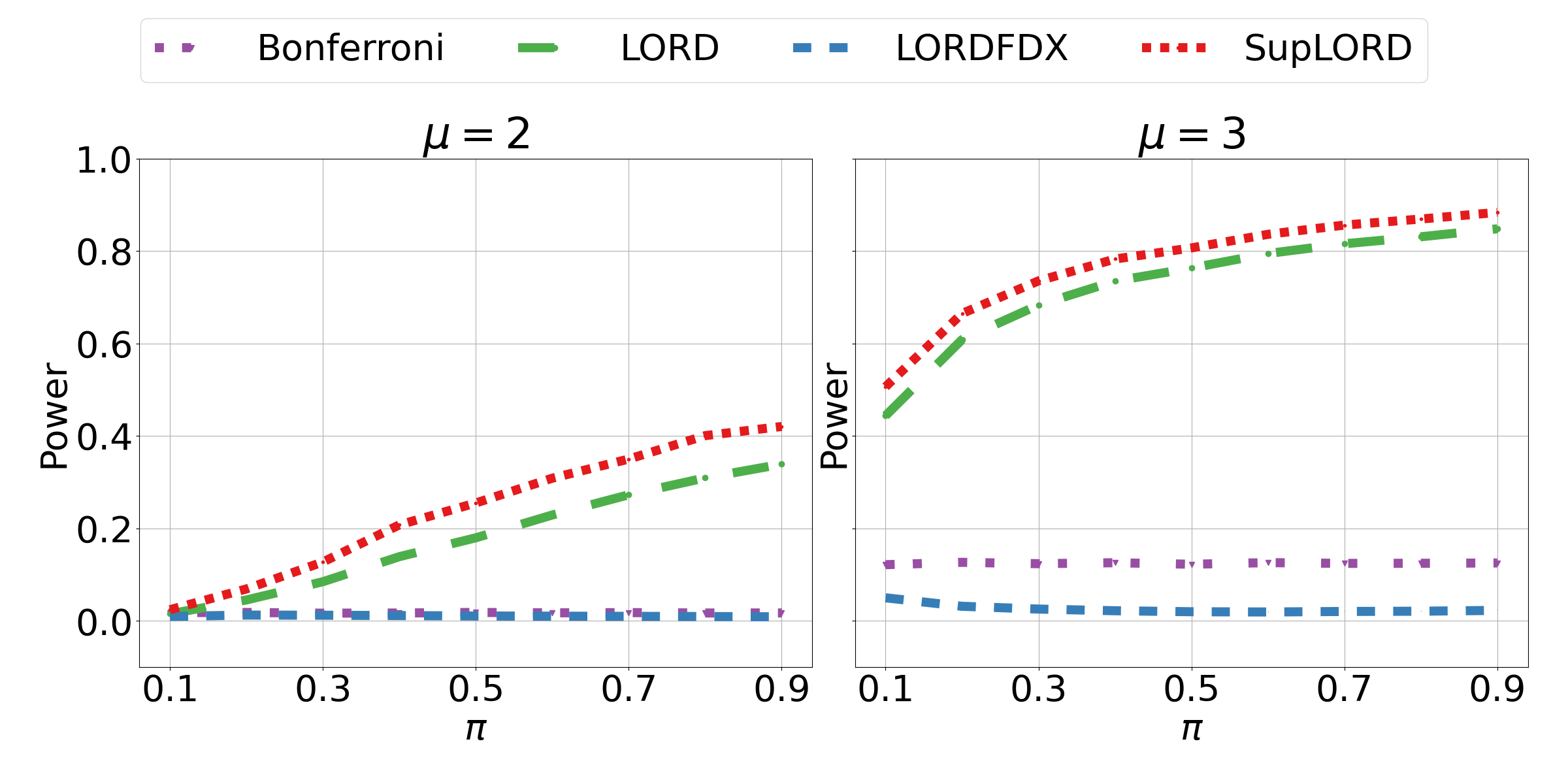
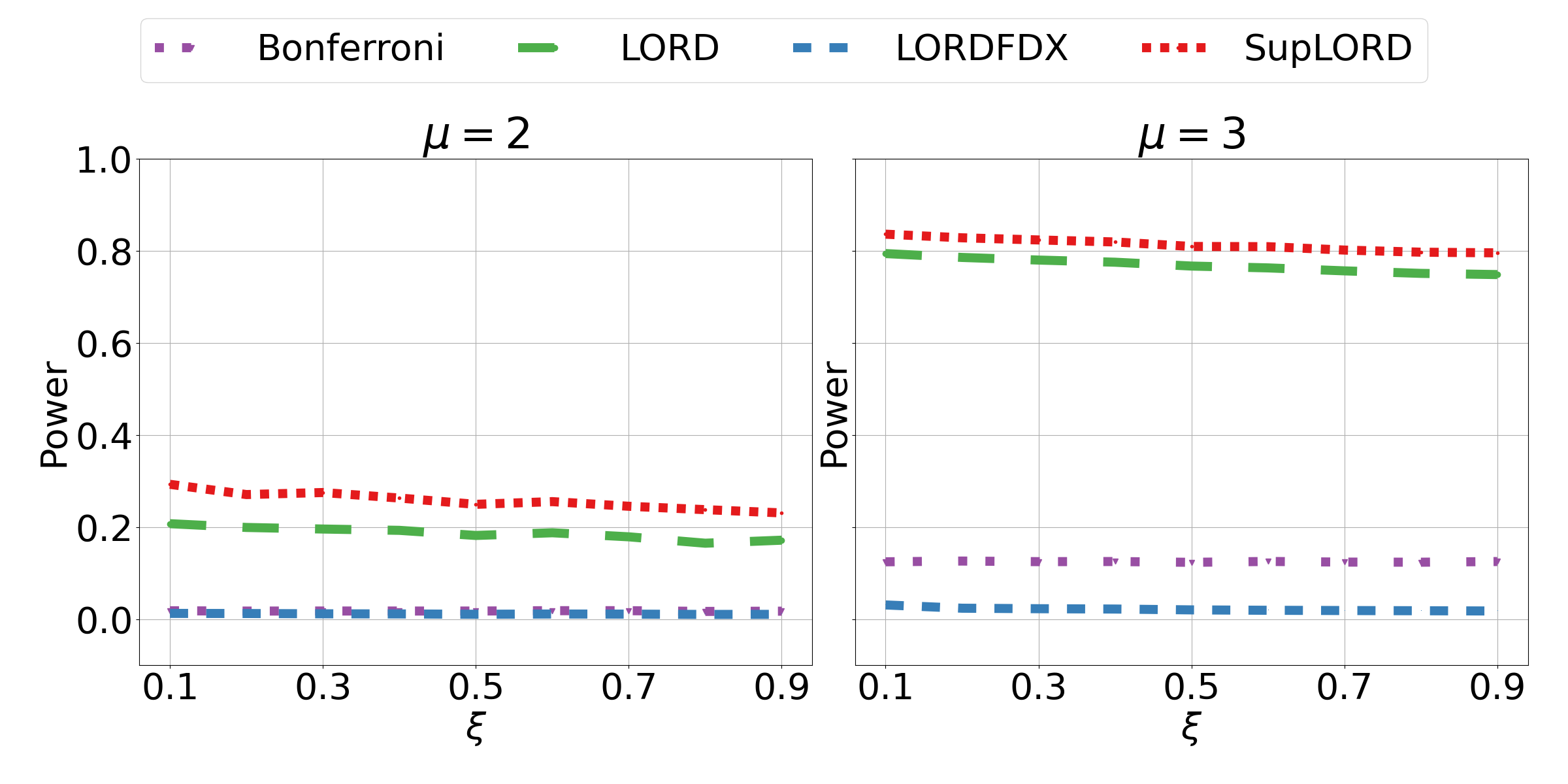
In Figure 3, we observe that the only other online FDXFDX\mathrm{FDX} control algorithm, LORDFDXLORDFDX\mathrm{LORD}\mathrm{FDX}, has significantly less power than SupLORDSupLORD\mathrm{SupLORD}. In fact, LORDFDXLORDFDX\mathrm{LORD}\mathrm{FDX} is on par or worse than the Bonferroni bound of alpha-spending. Thus, SupLORDSupLORD\mathrm{SupLORD} is able to obtain more power by delaying control for a constant number of rejections. Similar results are shown in the HMM setting, which we defer, along with additional metrics, to Appendix E. Further, these results are consistent with SupLORDSupLORD\mathrm{SupLORD} rejecting the most hypotheses on the IMPC data set in Table 2 — the gains in power seem to translate to a real world setting.

Table 2: Comparing total discoveries (rejected hypotheses) by each algorithm on the IMPC data. SupLORDSupLORD\mathrm{SupLORD} rejects the most hypotheses.
Method Rejections
Bonferroni 879
LORDLORD\mathrm{LORD} 12352
LORDFDXLORDFDX\mathrm{LORD}\mathrm{FDX} 8
SupLORDSupLORD\mathrm{SupLORD} 18793

Interestingly, these results also suggest a reversal of the previous notion that FDXFDX\mathrm{FDX} control was stricter than FDRFDR\mathrm{FDR} control. Previously, LORDFDXLORDFDX\mathrm{LORD}\mathrm{FDX} for controlling FDXFDX\mathrm{FDX} at some δsuperscript𝛿\delta^{*} was demonstrated by JM to be less powerful than LORDLORD\mathrm{LORD} controlling FDRFDR\mathrm{FDR} at a level of =δsuperscript𝛿\ell=\delta^{*} in experiments. This is due to LORDFDXLORDFDX\mathrm{LORD}\mathrm{FDX} being LORDLORD\mathrm{LORD} with an additional constraint i.e. if this additional constraint is violated, LORDFDXLORDFDX\mathrm{LORD}\mathrm{FDX} enters alpha-death. Hence, it is impossible for LORDFDXLORDFDX\mathrm{LORD}\mathrm{FDX} to make more rejections that LORDLORD\mathrm{LORD} when they are controlled at equivalent levels i.e. =δsuperscript𝛿\ell=\delta^{*}. On the other hand, SupLORDSupLORD\mathrm{SupLORD} uses the time-uniform bounds from KR to establish control of FDXFDX\mathrm{FDX}. SupLORDSupLORD\mathrm{SupLORD} suggests that controlling FDXFDX\mathrm{FDX} is not necessarily more restrictive than controlling FDRFDR\mathrm{FDR}. Since high probability bounds may be of greater interest to the user in practice, SupLORDSupLORD\mathrm{SupLORD} demonstrates that controlling FDXFDX\mathrm{FDX} does not necessarily sacrifice power.

Refer to caption
Figure 3: Plot of non-null likelihood, π𝜋\pi, vs. power for signal strengths of μ{2,3}𝜇23\mu\in\left\{2,3\right\}. FDRFDR\mathrm{FDR} is controlled at =0.050.05\ell=0.05, and SupLORDSupLORD\mathrm{SupLORD} and LORDFDXLORDFDX\mathrm{LORD}\mathrm{FDX} are controlled at FDXFDX\mathrm{FDX} with ϵ=0.15superscriptitalic-ϵ0.15\epsilon^{*}=0.15 at a level of δ=0.05superscript𝛿0.05\delta^{*}=0.05. Experiment details are in Section 3.2. SupLORDSupLORD\mathrm{SupLORD} consistently has higher power across all non-null likelihoods and signal strengths.

4 Dynamic Scheduling With Non-Monotone Spending Rules

Under-utilized wealth leads to unnecessary conservativeness.

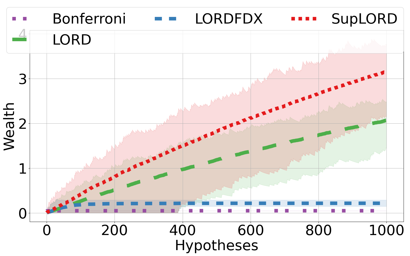
Recall that the wealth value at each step, W(k)𝑊𝑘W(k), quantifies the error budget that can be allocated to the next alpha value. Figure 4 shows that, empirically, the wealth increases as more hypotheses are tested when using steady with SupLORDSupLORD\mathrm{SupLORD} and LORDLORD\mathrm{LORD}. To the best of our knowledge, this problem of steady has not been addressed in previous work. The algorithm is not fully utilizing its error budget — the rate at which the algorithm is making rejections and accumulating wealth is much higher than the rate which wealth is spent. While aggressive does have better utilization of its wealth, it also does not distribute its spending as evenly as steady, since it spends a constant percentage of its current wealth at each step. To remedy this, we derive a new spending schedule that uses wealth much more rapidly when wealth has been accumulated. At the same time, we do not want our algorithm to spend excessively when wealth is scarce. Thus, our new spending schedule is adaptive to its wealth — it adjusts its rate of spending to evenly spend as much wealth as possible while avoiding alpha-death.

At a technical level, the underutilization of wealth occurs because prior alpha-spending rules are “monotone” (5) functions of past rejections, effectively handicapping them by making them unable to adapt to the current wealth. This monotonicity restriction was primarily imposed in order to mathematically prove FDR control, instead of mFDR control, in a proof technique introduced by Javanmard and Montanari (2018), and extended by all the followup works by Ramdas and coauthors. Our new proof technique avoids the requirement for monotonicity entirely, thus opening the possibility of designing smarter, wealth-adaptive spending rules, while still having FDX and FDR control.

4.1 Dynamic Scheduling Formulation

To address this problem, we provide a method for altering {γi}isubscriptsubscript𝛾𝑖𝑖\{\gamma_{i}\}_{i\in\mathbb{N}}, called dynamic scheduling, based on the wealth of the algorithm. The general paradigm of our new spending schedule is similar to the steady spending schedule in (13). In the steady spending schedule, we can see that each alpha value is the sum of portions of the wealth boosts at each past rejection. The portion of the wealth boost of the i𝑖ith rejection that the current alpha value spends is dependent on γktisubscript𝛾𝑘subscript𝑡𝑖\gamma_{k-t_{i}}, where k𝑘k is our current time, and tisubscript𝑡𝑖t_{i} is the time the i𝑖ith rejection was made. Our new spending schedule follows the same paradigm. However, we use a spending sequence that changes based upon the wealth of the algorithm at the time of the rejection, which we denote {γ¯i}isubscriptsubscript¯𝛾𝑖𝑖\{\overline{\gamma}_{i}\}_{i\in\mathbb{N}}. To create this, we must first have a base spending sequence {γi}isubscriptsubscript𝛾𝑖𝑖\{\gamma_{i}\}_{i\in\mathbb{N}}. Then, we formulate this new spending sequence as follows:

γ¯i(W,W(0))subscript¯𝛾𝑖𝑊𝑊0\displaystyle\overline{\gamma}_{i}(W,W(0)) {γiηWW(0)1j=1ργjηWW(0)1if ηWW(0)>1,iρ(active)0if ηWW(0)>1,i>ρ(active and finished)γielse (inactive),absentcasessuperscriptsubscript𝛾𝑖𝜂𝑊𝑊01superscriptsubscript𝑗1𝜌superscriptsubscript𝛾𝑗𝜂𝑊𝑊01formulae-sequenceif 𝜂𝑊𝑊01𝑖𝜌(active)0formulae-sequenceif 𝜂𝑊𝑊01𝑖𝜌(active and finished)subscript𝛾𝑖else (inactive)\displaystyle\equiv\begin{cases}\frac{\gamma_{i}^{\eta\cdot\frac{W}{W(0)}\vee 1}}{\sum\limits_{j=1}^{\rho}\gamma_{j}^{\eta\cdot\frac{W}{W(0)}\vee 1}}&\text{if }\eta\cdot\frac{W}{W(0)}>1,\ i\leq\rho\ \text{(active)}\\ 0&\text{if }\eta\cdot\frac{W}{W(0)}>1,\ i>\rho\ \text{(active and finished)}\\ \gamma_{i}&\text{else (inactive)},\end{cases} (16)

where W𝑊W and W(0)𝑊0W(0) are the wealth of the algorithm at the time of rejection and the beginning, respectively. γ¯isubscript¯𝛾𝑖\overline{\gamma}_{i} adapts to wealth by switching between the active and inactive cases. If the wealth is high when making a rejection, γ¯isubscript¯𝛾𝑖\overline{\gamma}_{i} goes into the active case where it spends wealth at a more rapid pace. Otherwise, it falls back to spending according to γisubscript𝛾𝑖\gamma_{i}. Figure 4 illustrates this adaptivity. η+𝜂superscript\eta\in\mathbb{R}^{+} controls the pace at which γ¯isubscript¯𝛾𝑖\overline{\gamma}_{i} spends wealth as a function the algorithm’s current wealth. ρ𝜌\rho\in\mathbb{N} controls the length of time before γ¯isubscript¯𝛾𝑖\overline{\gamma}_{i} has exhausted the wealth earned from its rejection — the first ρ𝜌\rho elements of γisubscript𝛾𝑖\gamma_{i} are normalized to create γ¯isubscript¯𝛾𝑖\overline{\gamma}_{i}. Larger η𝜂\eta and smaller ρ𝜌\rho increases spending in the active case. Note that γ¯isubscript¯𝛾𝑖\overline{\gamma}_{i} satisfy conditions (12), making it a valid spending sequence.

\subfigure

[Wealth of different GAI algorithms (setting specified in Section 3.2). The line is the mean over 200 trials and the shaded area is a 95% confidence set. SupLORDSupLORD\mathrm{SupLORD} and LORDLORD\mathrm{LORD} both have increasing wealth.] Refer to caption   \subfigure[Visualization of γ¯isubscript¯𝛾𝑖\overline{\gamma}_{i} vs γisubscript𝛾𝑖\gamma_{i} in (16). γ¯isubscript¯𝛾𝑖\overline{\gamma}_{i} is only active for ρ𝜌\rho duration and is much larger than γisubscript𝛾𝑖\gamma_{i} during that duration, which results in increased spending.] Refer to caption
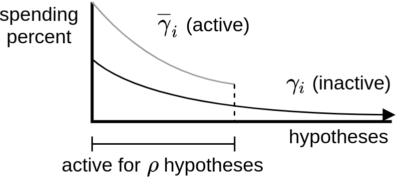
Figure 4: Visualization of concepts pertaining to dynamic scheduling.

Thus, using γ¯isubscript¯𝛾𝑖\overline{\gamma}_{i} allows for the spending schedule to quickly use up entire boosts in wealth from rejections if the current wealth of the algorithm is large. We define our dynamic alpha schedule as:

αk=γ¯k(W(0),W(0))β0+i=1|k1|γ¯kti(W(ti),W(0))βti.subscript𝛼𝑘subscript¯𝛾𝑘𝑊0𝑊0subscript𝛽0superscriptsubscript𝑖1subscript𝑘1subscript¯𝛾𝑘subscript𝑡𝑖𝑊subscript𝑡𝑖𝑊0subscript𝛽subscript𝑡𝑖\displaystyle\alpha_{k}=\overline{\gamma}_{k}(W(0),W(0))\cdot\beta_{0}+\sum\limits_{i=1}^{\left|\mathcal{R}_{k-1}\right|}\overline{\gamma}_{k-t_{i}}(W(t_{i}),W(0))\cdot\beta_{t_{i}}. (17)

We will show through simulation results that this method does solve the problem of wealth under-utilization and increases the power of SupLORDSupLORD\mathrm{SupLORD} as a result.

4.2 Numerical Simulations and Real Data Experiments for Dynamic Algorithms

Spending schedules.

We compare the differences in steady, aggressive, and dynamic scheduling on SupLORDSupLORD\mathrm{SupLORD}. We choose ϵ=0.15,δ=0.05,r=30formulae-sequencesuperscriptitalic-ϵ0.15formulae-sequencesuperscript𝛿0.05superscript𝑟30\epsilon^{*}=0.15,\ \delta^{*}=0.05,\ r^{*}=30 as the parameters for simulations, and r=100superscript𝑟100r^{*}=100 for the IMPC dataset in all SupLORDSupLORD\mathrm{SupLORD} algorithms. We use the default boost sequence and spending sequence for all three schedules.

Results for comparing spending schedules.

\subfigure

[Non-null likelihood π𝜋\pi vs. power] Refer to caption \subfigure[Wealth vs. time] Refer to caption

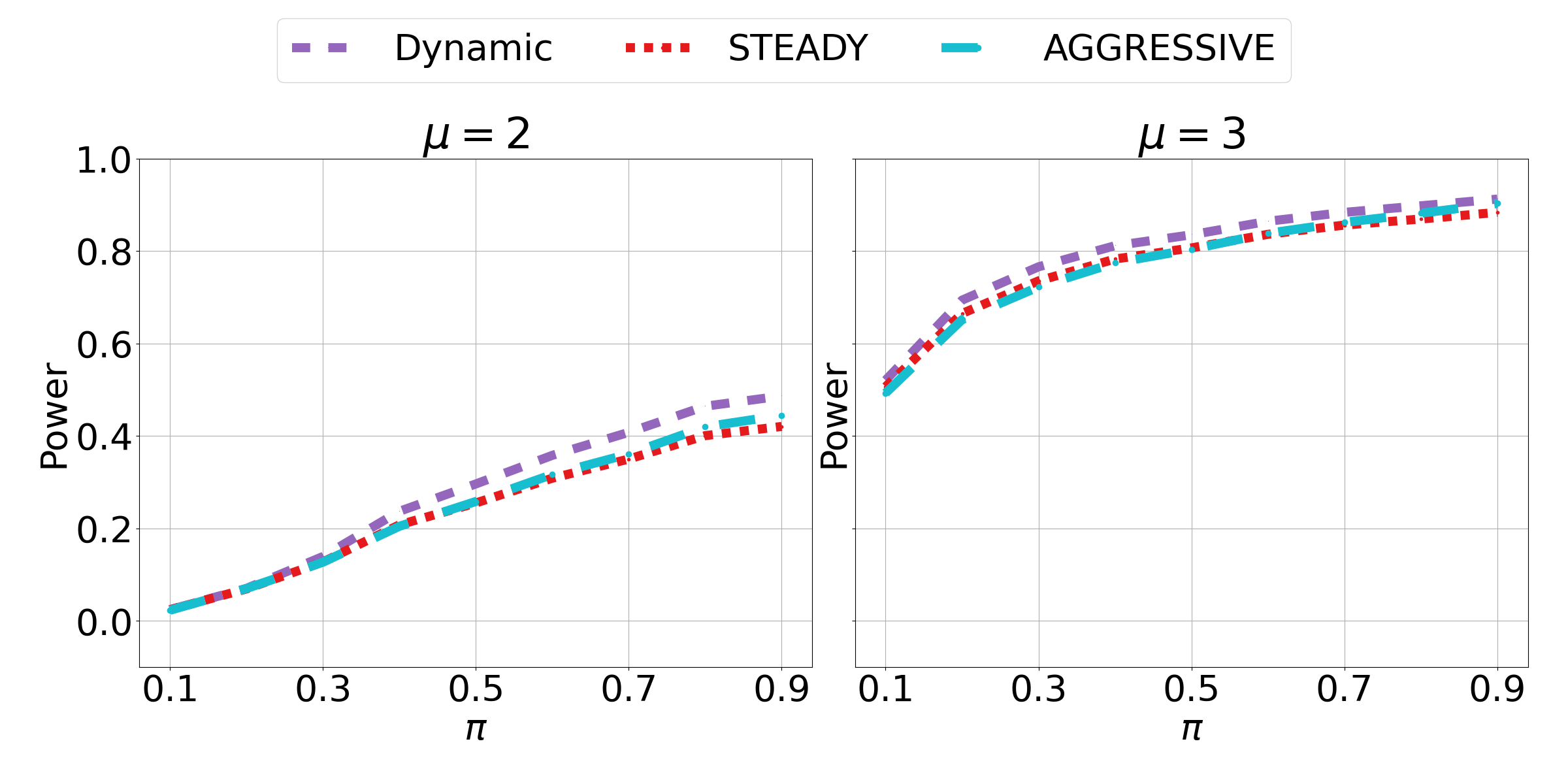
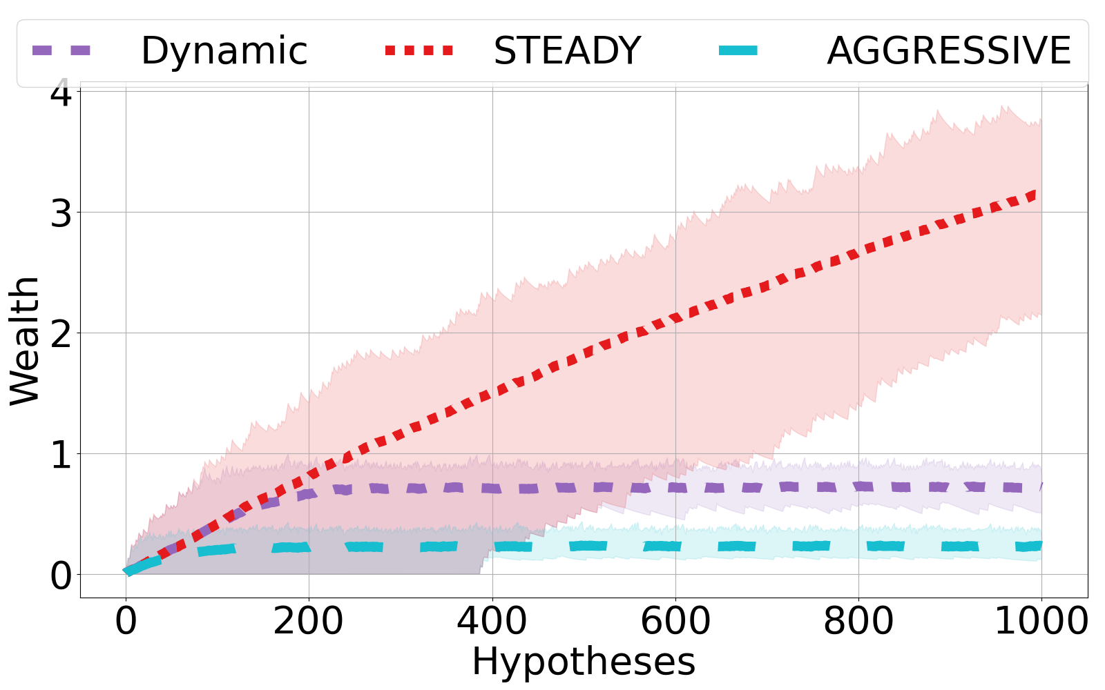
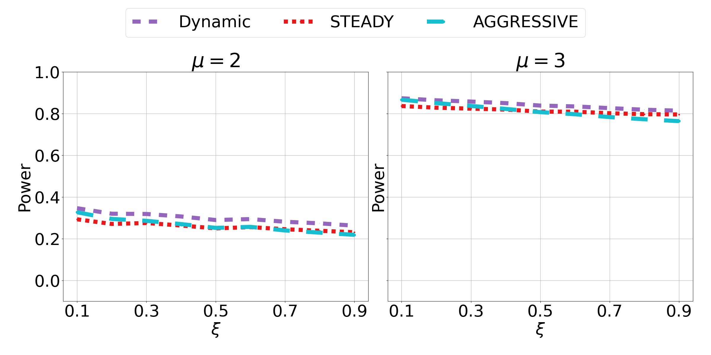
Figure 5: The left plot compares different spending schedule choices for SupLORDSupLORD\mathrm{SupLORD} plotted by likelihood of non-null hypotheses, π𝜋\pi, vs. power for signal strengths of μ{2,3}𝜇23\mu\in\left\{2,3\right\} in the manner specified in Section 3.2. Dynamic scheduling provides a consistent (albeit small) power improvement over steady and aggressive SupLORDSupLORD\mathrm{SupLORD}. The right plot shows that the dynamic scheduling does not hoard wealth like steady, but saves more than aggressive.
Table 3: Rejections made by each schedule on the IMPC data. Dynamic scheduling has the most rejections.
Schedule Rejections
steady 18519
aggressive 15416
dynamic 18793

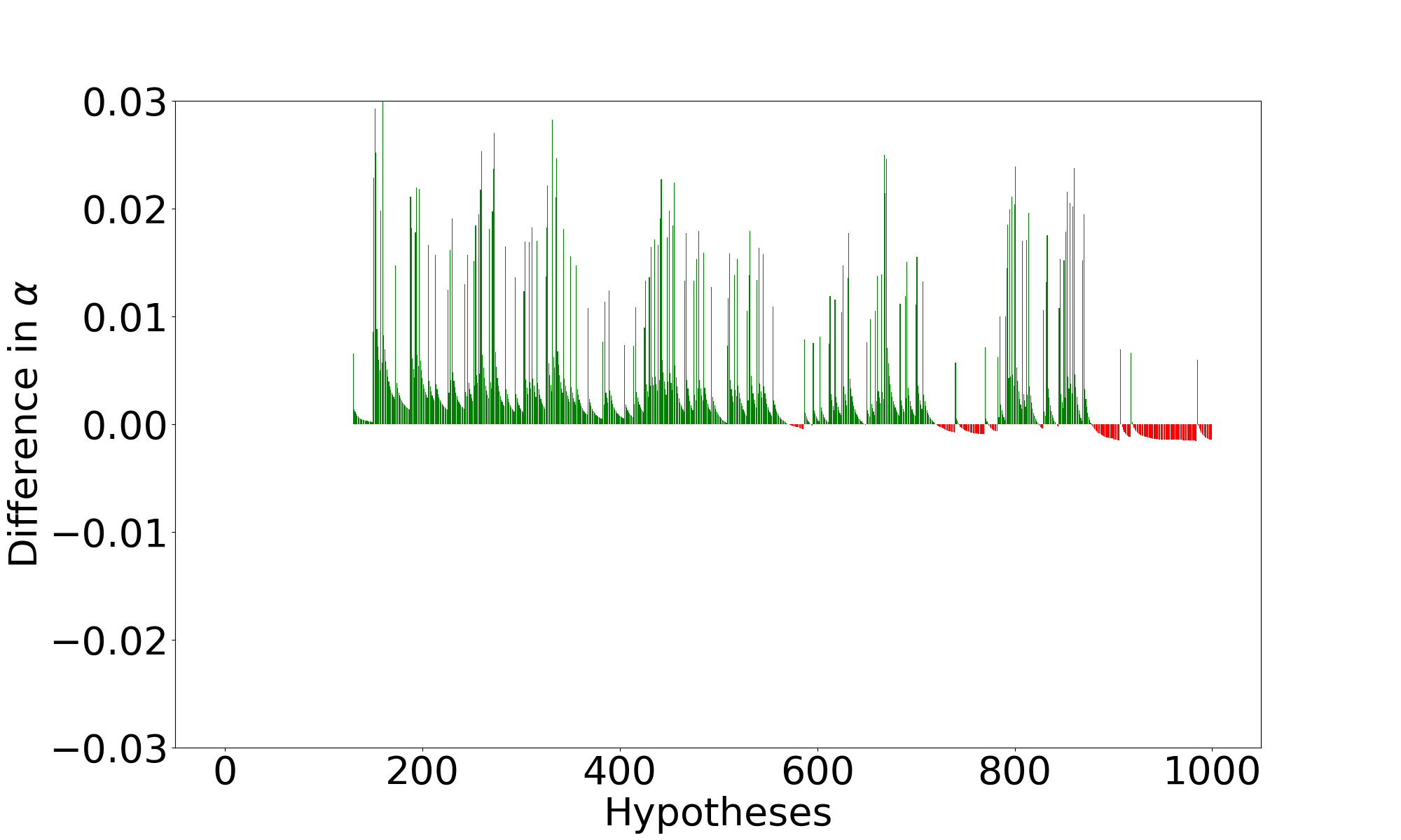
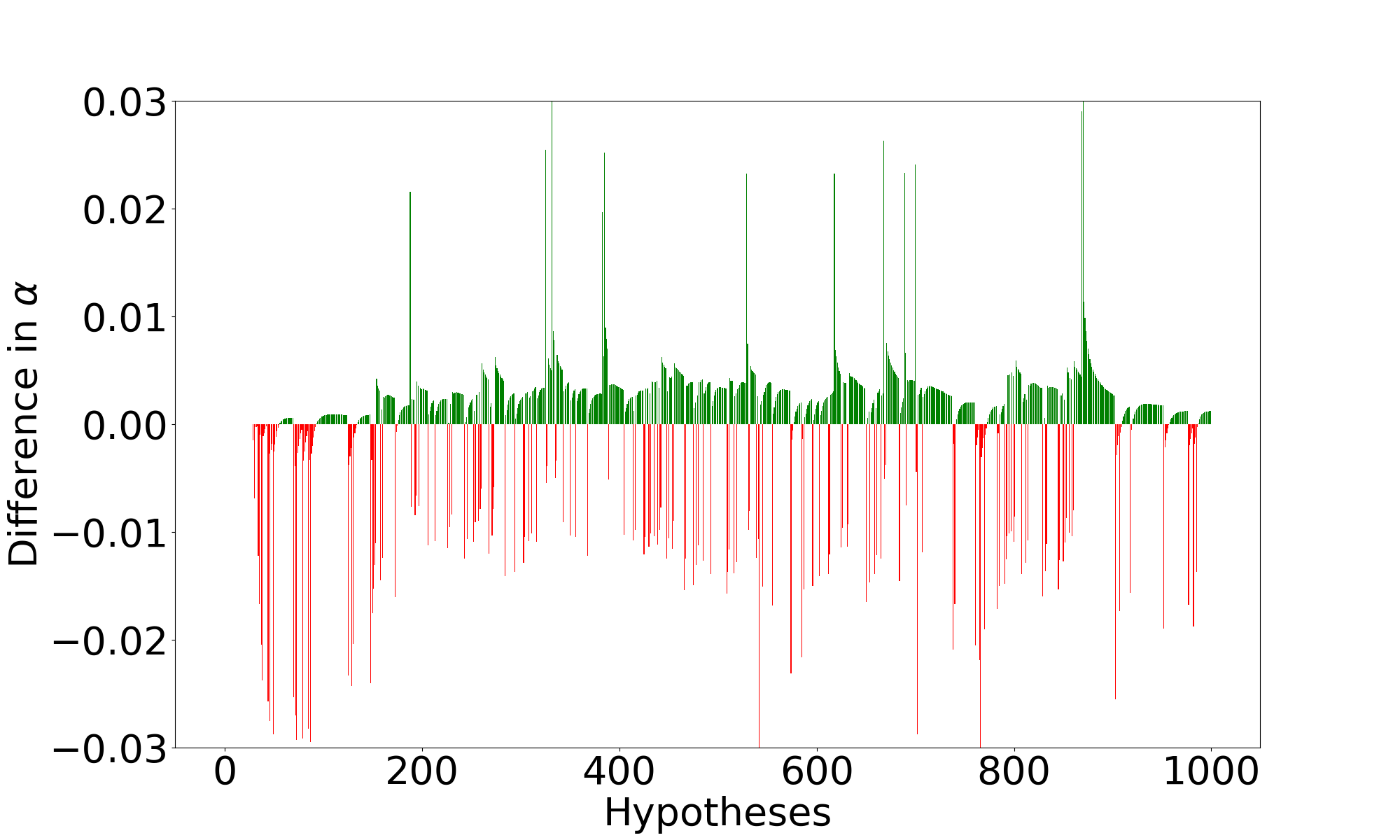
Figure 5 shows that using a dynamic schedule does increase power when the signal and likelihood of the non-null hypotheses are larger, and does not do worse than the steady or aggressive when the signal and likelihood of non-nulls are low. This corresponds to the formulation of the γ¯isubscript¯𝛾𝑖\overline{\gamma}_{i}, as it falls back to γisubscript𝛾𝑖\gamma_{i} if the algorithm’s wealth is low. In the largest settings of non-null likelihood and signal, aggressive catches up to dynamic scheduling in power. Admittedly, dynamic scheduling is limited in its power gains, since it only allocates existing wealth more effectively. Yet, it still outperforms both baseline schedules across simulation settings — we illustrate that dynamic scheduling generally produces larger alpha values than either baseline schedule in Appendix F. Further, a dynamic schedule also makes more rejections than other schedules on the IMPC dataset in Table 3, which is consistent with its power improvement in simulations. Thus, a dynamic schedule fully utilizes wealth and is a good default for practitioners.

5 Improving FDRFDR\mathrm{FDR} Control Through SupFDRSupFDR\mathrm{SupFDR} Control

Finally, we illustrate the connections between FDRFDR\mathrm{FDR}, FDXFDX\mathrm{FDX}, and SupFDRSupFDR\mathrm{SupFDR}. We use additional results from KR to prove that SupLORDSupLORD\mathrm{SupLORD} controls the SupFDRSupFDR\mathrm{SupFDR}, and by extension, FDRFDR\mathrm{FDR}. These FDRFDR\mathrm{FDR} results close the gap between FDRFDR\mathrm{FDR} control and mFDRmFDR\mathrm{mFDR} control (4), which was first introduced by FS as a proxy for FDRFDR\mathrm{FDR}. FS showed that mFDR(τ)mFDRsubscript𝜏\mathrm{mFDR}(\mathcal{R}_{\tau}), where τ𝜏\tau is a stopping time with respect to {k}subscript𝑘\{\mathcal{F}_{k}\}, could be controlled under assumption (2). One example of a stopping time is the time of the k𝑘k-th rejection, for some fixed k𝑘k\in\mathbb{N}. Successive works (JM, Ramdas et al. 2017) have managed to show FDRFDR\mathrm{FDR} control with more restrictive assumptions of (3) and monotone spending schedules.333Technically, JM do have a theorem that proves FDRFDR\mathrm{FDR} control for dependent p-variables, but it is dependent on a strict uniformity assumption and also suffers from alpha-death since the proportion of wealth it can spend at each step is inversely proportional to the logarithm of the number of hypotheses that have been tested. In addition, they also have only controlled at FDRFDR\mathrm{FDR} fixed times, unlike the stopping time control of mFDRmFDR\mathrm{mFDR} proved by FS. Thus, SupLORDSupLORD\mathrm{SupLORD} completes the original goal of FS by showing control, under the same assumptions, on the actual desired metric, FDRFDR\mathrm{FDR}, for stopping times. To prove this, we first note SupLORDSupLORD\mathrm{SupLORD} provides a family of FDXFDX\mathrm{FDX} bounds by 1.

Corollary 1 (Corollary of Theorem 1).

Assuming conditional superuniformity (2), any GAI algorithm that satisfies conditions (14) also ensures the following family of bounds for any δ(0,1)𝛿01\delta\in(0,1):

FDXtr(log¯(1δ)log¯(1δ)ϵ)δ.subscriptFDXsubscript𝑡superscript𝑟¯1𝛿¯1superscript𝛿superscriptitalic-ϵ𝛿\displaystyle\mathrm{FDX}_{t_{r^{*}}}\left(\frac{{\overline{\log}}{\left(\frac{1}{\delta}\right)}}{{\overline{\log}}{\left(\frac{1}{\delta^{*}}\right)}}\epsilon^{*}\right)~{}\leq~{}\delta.

Before we state our control of SupFDRSupFDR\mathrm{SupFDR}, we will introduce the following constant:

c𝑐\displaystyle c =01log¯(1δ)𝑑δ1.419.absentsuperscriptsubscript01¯1𝛿differential-d𝛿1.419\displaystyle=\int\limits_{0}^{1}{\overline{\log}}{\left(\frac{1}{\delta}\right)}\ d\delta\approx 1.419~{}.
Theorem 2.

Assuming conditional superuniformity (2), any GAI algorithm that satisfies conditions (14) ensures the following bound holds:

SupFDRtrcϵlog¯(1δ).subscriptSupFDRsubscript𝑡superscript𝑟𝑐superscriptitalic-ϵ¯1superscript𝛿\displaystyle\mathrm{SupFDR}_{t_{r^{*}}}~{}\leq~{}\frac{c\epsilon^{*}}{{\overline{\log}}{\left(\frac{1}{\delta^{*}}\right)}}.

A detailed proof is provided in Appendix B of the supplement. Intuitively, we can achieve this expectation by integrating over the family of FDXFDX\mathrm{FDX} bounds described in Corollary 1. Thus, this theorem establishes a connection between controlling FDXFDX\mathrm{FDX} and SupFDRSupFDR\mathrm{SupFDR} for SupLORDSupLORD\mathrm{SupLORD}. Unlike prior FDRFDR\mathrm{FDR} bounds which are only valid at fixed times, Theorem 2 provides a bound on FDRFDR\mathrm{FDR} for stopping times. Formally, a stopping time τ𝜏\tau is a random variable where the event τ=k𝜏𝑘\tau=k is measurable in ksubscript𝑘\mathcal{F}_{k} for all k𝑘k. Due to the supremum in Theorem 2, we may derive the following corollary:

Corollary 2.

Assuming conditional superuniformity (2), τ𝜏\tau is a stopping time that satisfies τtr𝜏subscript𝑡superscript𝑟\tau\geq t_{r^{*}}, any GAI algorithm that satisfies conditions (14) ensures the following bounds hold:

FDR(τ)cϵlog¯(1δ).FDRsubscript𝜏𝑐superscriptitalic-ϵ¯1superscript𝛿\displaystyle\mathrm{FDR}(\mathcal{R}_{\tau})~{}\leq~{}\frac{c\epsilon^{*}}{{\overline{\log}}{\left(\frac{1}{\delta^{*}}\right)}}.

Thus, using SupLORDSupLORD\mathrm{SupLORD} provides the benefit of maintaining FDRFDR\mathrm{FDR} control even when the user may desire to adaptively stop testing hypotheses, and lends flexibility to its usage as a result. Since this result follows directly from Theorem 2, it does not require any extra assumptions besides conditional superuniformity (2). In contrast, prior online FDR methods (Ramdas et al. 2017, 2018, JM) require stronger assumptions of independence (3) and monotone spending schedules (5). Further, they only control FDRFDR\mathrm{FDR} at fixed times. Consequently, Corollary 2 improves upon prior work in both the generality of its assumptions and the strength of its guarantee. Additional SupLORDSupLORD\mathrm{SupLORD} guarantees are discussed in Appendix C (tighter FDRFDR\mathrm{FDR} control at fixed times) and Appendix D (mFDRmFDR\mathrm{mFDR} control at stopping times).

6 Related Work on Online Multiple Testing

Online multiple testing was introduced by FS (Foster and Stine, 2008), which formulated the problem and setup, and the first algorithm better than a Bonferroni bound through the paradigm of “alpha-investing”. Notably, FS introduced the notion of mFDRmFDR\mathrm{mFDR} and proved control at stopping times for mFDRmFDR\mathrm{mFDR} in this work because they found FDRFDR\mathrm{FDR} control difficult to prove. Aharoni and Rosset (2014) extended the guarantees from FS to a broader class of algorithms. The LORDLORD\mathrm{LORD} algorithm formulated by JM (Javanmard and Montanari, 2018) is a particularly powerful type of GAI algorithm, and JM showed it could control FDRFDR\mathrm{FDR} at all fixed times — this was consequently the first substantial FDRFDR\mathrm{FDR} control result in the area. In fact, Chen and Arias-Castro (2020) proved that LORDLORD\mathrm{LORD} is asymptotically as powerful as the best offline algorithm for controlling FDRFDR\mathrm{FDR}. Ramdas et al. (2017) then relaxed the conditions for FDRFDR\mathrm{FDR} control in LORDLORD\mathrm{LORD} and formulated a family of algorithms, known as GAI++, that improved power over any GAI algorithm, including LORDLORD\mathrm{LORD}. For instances of application, Xu et al. (2015) provide a comprehensive overview of how online hypothesis testing plays a crucial in modern A/B testing. Robertson and Wason (2018); Robertson et al. (2019) apply the problem in a biomedical setting.

Several works have improved the power of the LORD++\mathrm{LORD}++ algorithm (Tian and Ramdas, 2019; Ramdas et al., 2018). This paper’s methods are not specific to LORDLORD\mathrm{LORD} — we may generalize dynamic scheduling to any generalized alpha-investing algorithm and the FDXFDX\mathrm{FDX} control obtained by SupLORDSupLORD\mathrm{SupLORD} can also be applied to algorithms with other FDPFDP\mathrm{FDP} estimators, like the one in Ramdas et al. (2018).

Other related work on online selective inference includes online methods for controlling family-wise error rate (Tian and Ramdas, 2021), false coverage rate (Weinstein and Ramdas, 2020), and FDRFDR\mathrm{FDR} in minibatches i.e. neighboring batches of hypotheses also have FDRFDR\mathrm{FDR} control (Zrnic et al., 2020). Controlling any of these metrics guarantees control of the FDRFDR\mathrm{FDR} as well. Zrnic et al. (2021) considers FDRFDR\mathrm{FDR} control under local dependence between p-values. Gang et al. (2020) take a Bayesian approach to the problem and increase the power of their algorithms by exploiting local structure.

All aforementioned works are primarily concerned with error control in expectation and thus are focused on controlling the FDRFDR\mathrm{FDR}. In contrast, this paper introduces an first empirically powerful algorithm, SupLORDSupLORD\mathrm{SupLORD}, for controlling the FDPFDP\mathrm{FDP} at a set level with high probability i.e. FDXFDX\mathrm{FDX}. Further, control at stopping times has only been shown for mFDRmFDR\mathrm{mFDR} by FS and Aharoni and Rosset (2014). SupLORDSupLORD\mathrm{SupLORD} is the first algorithm to demonstrate any control of FDRFDR\mathrm{FDR} at stopping times. Thus, SupLORDSupLORD\mathrm{SupLORD} broadens the online multiple testing literature to account for FDXFDX\mathrm{FDX} control and fills the existing gap of controlling FDRFDR\mathrm{FDR} at stopping times.

7 Summary

We have shown a new algorithm, SupLORDSupLORD\mathrm{SupLORD}, that controls FDXFDX\mathrm{FDX} and is empirically more powerful by a significant amount than previous FDXFDX\mathrm{FDX} controlling algorithms. We also show that SupLORDSupLORD\mathrm{SupLORD} may simultaneously control FDXFDX\mathrm{FDX}, FDRFDR\mathrm{FDR}, and SupFDRSupFDR\mathrm{SupFDR} together. In addition, we make the observation that existing algorithms are not tight to their level of error control, and formulate dynamic scheduling, a framework for adapting to the wealth of an algorithm. We empirically show that dynamic scheduling increases power and reduces this wealth gap. Thus, we formulated the most powerful algorithms for FDXFDX\mathrm{FDX} control and brought insight to the interplay between multiple error metrics in this paper. Finally, our paper showed the first non-trivial algorithm with FDRFDR\mathrm{FDR} control at stopping times, filling a gap in the literature that had been noticed by FS when they first proposed the problem. We plan on implementing our methods and incorporating them into the onlineFDR R package (Robertson et al., 2019), which contains current state-of-the-art online multiple testing algorithms. One line for future work is understanding how η𝜂\eta and ρ𝜌\rho can be set optimally in dynamic scheduling, and whether there is choice of parameters that is provably most powerful or optimal in some sense.

Acknowledgements

We would like to thank our anonymous reviewers for their suggestions and questions. AR acknowledges support from NSF CAREER 1945266.

References

  • Aharoni and Rosset (2014) E. Aharoni and S. Rosset. Generalized α𝛼\alpha-investing: definitions, optimality results and application to public databases. Journal of the Royal Statistical Society: Series B: Statistical Methodology, pages 771–794, 2014.
  • Chen and Arias-Castro (2020) S. Chen and E. Arias-Castro. On the power of some sequential multiple testing procedures. Annals of the Institute of Statistical Mathematics, Apr. 2020. ISSN 0020-3157, 1572-9052. doi: 10.1007/s10463-020-00752-5.
  • Foster and Stine (2008) D. Foster and R. A. Stine. Alpha-Investing: A Procedure for Sequential Control of Expected False Discoveries. Journal of the Royal Statistical Society: Series B: Statistical Methodology, 70(2):429, 2008.
  • Gang et al. (2020) B. Gang, W. Sun, and W. Wang. Structure-Adaptive Sequential Testing for Online False Discovery Rate Control. arXiv:2003.00113 [stat], Feb. 2020.
  • Javanmard and Montanari (2018) A. Javanmard and A. Montanari. Online rules for control of false discovery rate and false discovery exceedance. The Annals of Statistics, 46(2):526–554, 2018.
  • Karp et al. (2017) N. A. Karp, J. Mason, A. L. Beaudet, Y. Benjamini, L. Bower, R. E. Braun, S. D. M. Brown, E. J. Chesler, M. E. Dickinson, A. M. Flenniken, H. Fuchs, M. H. de Angelis, X. Gao, S. Guo, S. Greenaway, R. Heller, Y. Herault, M. J. Justice, N. Kurbatova, C. J. Lelliott, K. C. K. Lloyd, A.-M. Mallon, J. E. Mank, H. Masuya, C. McKerlie, T. F. Meehan, R. F. Mott, S. A. Murray, H. Parkinson, R. Ramirez-Solis, L. Santos, J. R. Seavitt, D. Smedley, T. Sorg, A. O. Speak, K. P. Steel, K. L. Svenson, S. Wakana, D. West, S. Wells, H. Westerberg, S. Yaacoby, and J. K. White. Prevalence of sexual dimorphism in mammalian phenotypic traits. Nature Communications, 8(1):15475, June 2017. ISSN 2041-1723. doi: 10.1038/ncomms15475.
  • Katsevich and Ramdas (2020) E. Katsevich and A. Ramdas. Simultaneous high-probability bounds on the false discovery proportion in structured, regression and online settings. Ann. Statist., 48(6):3465–3487, 12 2020. doi: 10.1214/19-AOS1938. URL https://doi.org/10.1214/19-AOS1938.
  • Ramdas et al. (2017) A. Ramdas, F. Yang, M. J. Wainwright, and M. I. Jordan. Online control of the false discovery rate with decaying memory. In Advances In Neural Information Processing Systems, pages 5650–5659, 2017.
  • Ramdas et al. (2018) A. Ramdas, T. Zrnic, M. Wainwright, and M. Jordan. SAFFRON: an adaptive algorithm for online control of the false discovery rate. In International Conference on Machine Learning, pages 4286–4294, 2018.
  • Robertson and Wason (2018) D. S. Robertson and J. Wason. Online control of the false discovery rate in biomedical research. arXiv preprint arXiv:1809.07292, 2018.
  • Robertson et al. (2019) D. S. Robertson, L. Liou, A. Ramdas, A. Javanmard, J. Tian, T. Zrnic, and N. A. Karp. onlineFDR: Online error control, 2019. R package 1.7.1.
  • Tian and Ramdas (2019) J. Tian and A. Ramdas. ADDIS: an adaptive discarding algorithm for online FDR control with conservative nulls. In Advances in Neural Information Processing Systems, pages 9388–9396, 2019.
  • Tian and Ramdas (2021) J. Tian and A. Ramdas. Online control of the familywise error rate. Statistical Methods in Medical Research, 2021. ISSN 0962-2802. doi: 10.1177/0962280220983381.
  • Wasserman (2004) L. Wasserman. All of Statistics: A Concise Course in Statistical Inference. Springer Science & Business Media, Sept. 2004. ISBN 978-0-387-40272-7.
  • Weinstein and Ramdas (2020) A. Weinstein and A. Ramdas. Online control of the false coverage rate and false sign rate. In International Conference on Machine Learning, 2020.
  • Xu et al. (2015) Y. Xu, N. Chen, A. Fernandez, O. Sinno, and A. Bhasin. From infrastructure to culture: A/B testing challenges in large scale social networks. In Proceedings of the 21th ACM SIGKDD International Conference on Knowledge Discovery and Data Mining, pages 2227–2236, 2015.
  • Zrnic et al. (2020) T. Zrnic, D. Jiang, A. Ramdas, and M. Jordan. The Power of Batching in Multiple Hypothesis Testing. In International Conference on Artificial Intelligence and Statistics, pages 3806–3815, 2020.
  • Zrnic et al. (2021) T. Zrnic, A. Ramdas, and M. I. Jordan. Asynchronous Online Testing of Multiple Hypotheses. Journal of Machine Learning Research, 22(33):1–39, 2021. ISSN 1533-7928.

Appendix A SupLORDSupLORD\mathrm{SupLORD} General Formulation

We first define a more general form of SupLORDSupLORD\mathrm{SupLORD} that is valid for any γ,rsuperscript𝛾superscript𝑟\gamma^{*},r^{*}. We add an additional user parameter of a>0𝑎0a>0. We now redefine our estimators of FDPFDP\mathrm{FDP} to include a𝑎a.

FDP^a(k)subscript^FDP𝑎subscript𝑘\displaystyle\widehat{\mathrm{FDP}}_{a}(\mathcal{R}_{k}) V^k+a|k|,absentsubscript^𝑉𝑘𝑎subscript𝑘\displaystyle~{}\equiv~{}\frac{\widehat{V}_{k}+a}{\left|\mathcal{R}_{k}\right|},
log¯[a](1δ)subscript¯delimited-[]𝑎1𝛿\displaystyle{\overline{\log}_{\left[a\right]}}{\left(\frac{1}{\delta}\right)} log(1δ)alog(1+log(1δ)a),absent1𝛿𝑎11𝛿𝑎\displaystyle~{}\equiv~{}\frac{\log(\frac{1}{\delta})}{a\log\left(1+\frac{\log(\frac{1}{\delta})}{a}\right)}~{},
FDP¯a(k)subscript¯FDP𝑎subscript𝑘\displaystyle\overline{\mathrm{FDP}}_{a}(\mathcal{R}_{k}) log¯[a](1δ)FDP^a(k).absentsubscript¯delimited-[]𝑎1𝛿subscript^FDP𝑎subscript𝑘\displaystyle~{}\equiv~{}{\overline{\log}_{\left[a\right]}}{\left(\frac{1}{\delta}\right)}\cdot\widehat{\mathrm{FDP}}_{a}(\mathcal{R}_{k}).

We drop a𝑎a from the notation when a=1𝑎1a=1. We first cite the more general form of 1.

Fact 2 (Detailed form of Theorem 4 from KR).

Let {αk}ksubscriptsubscript𝛼𝑘𝑘\{\alpha_{k}\}_{k\in\mathbb{N}} be any sequence of alpha values predictable with respect to filtration ksubscript𝑘\mathcal{F}_{k} in definition (1). Assuming conditional superuniformity (2), the following uniform bound holds:

𝐏𝐫(FDP(k)FDP¯a(k) for all k1)1δ.𝐏𝐫FDPsubscript𝑘subscript¯FDP𝑎subscript𝑘 for all 𝑘11𝛿\displaystyle\mathbf{Pr}\left(\mathrm{FDP}(\mathcal{R}_{k})\leq\overline{\mathrm{FDP}}_{a}(\mathcal{R}_{k})\text{ for all }k\geq 1\right)\geq 1-\delta.

Consequently, our conditions on the boost sequence {βi}i{0}subscriptsubscript𝛽𝑖𝑖0\{\beta_{i}\}_{i\in\mathbb{N}\cup\{0\}} is modified to account for a𝑎a:

i=0tr1βiRisuperscriptsubscript𝑖0subscript𝑡superscript𝑟1subscript𝛽𝑖subscript𝑅𝑖\displaystyle\sum\limits_{i=0}^{t_{r^{*}-1}}\beta_{i}R_{i} ϵrlog¯[a](1δ)aabsentsuperscriptitalic-ϵsuperscript𝑟subscript¯delimited-[]𝑎1superscript𝛿𝑎\displaystyle\leq\frac{\epsilon^{*}r^{*}}{{\overline{\log}_{\left[a\right]}}{\left(\frac{1}{\delta^{*}}\right)}}-a (18a)
βisubscript𝛽𝑖\displaystyle\beta_{i} ϵlog¯[a](1δ)for all i>tr1.absentsuperscriptitalic-ϵsubscript¯delimited-[]𝑎1superscript𝛿for all 𝑖subscript𝑡superscript𝑟1\displaystyle\leq\frac{\epsilon^{*}}{{\overline{\log}_{\left[a\right]}}{\left(\frac{1}{\delta^{*}}\right)}}\ \text{for all }i>t_{r^{*}-1}. (18b)

The default {βi}i{0}subscriptsubscript𝛽𝑖𝑖0\{\beta_{i}\}_{i\in\mathbb{N}\cup\{0\}} can be specified as follows:

βi={1r(ϵrlog¯[a](1δ)a)i<r,ϵlog¯[a](1δ)ir.subscript𝛽𝑖cases1superscript𝑟superscriptitalic-ϵsuperscript𝑟subscript¯delimited-[]𝑎1superscript𝛿𝑎𝑖superscript𝑟superscriptitalic-ϵsubscript¯delimited-[]𝑎1superscript𝛿𝑖superscript𝑟\displaystyle\beta_{i}=\begin{cases}\frac{1}{r^{*}}\left(\frac{\epsilon^{*}r^{*}}{{\overline{\log}_{\left[a\right]}}{\left(\frac{1}{\delta^{*}}\right)}}-a\right)&i<r^{*},\\ \frac{\epsilon^{*}}{{\overline{\log}_{\left[a\right]}}{\left(\frac{1}{\delta^{*}}\right)}}&i\geq r^{*}\end{cases}\quad. (19)

Choosing a=1𝑎1a=1 recovers conditions (14) and the default sequence in (15).

Naturally, the we then prove the following bound holds for the general form:

Theorem 3.

Given that conditional superuniformity (2) holds, let 0<ϵ,δ<1formulae-sequence0superscriptitalic-ϵsuperscript𝛿10<\epsilon^{*},\delta^{*}<1, r1superscript𝑟1r^{*}\geq 1 be a positive integer, and trsubscript𝑡superscript𝑟t_{r^{*}} be a random variable that is the time when the rsuperscript𝑟r^{*}th rejection is made. A GAI algorithm with a boost sequence {βi}i{0}subscriptsubscript𝛽𝑖𝑖0\{\beta_{i}\}_{i\in\mathbb{N}\cup\{0\}} that satisfies conditions (18) guarantees:

FDXtrϵδ.superscriptsubscriptFDXsuperscriptsubscript𝑡𝑟superscriptitalic-ϵsuperscript𝛿\displaystyle\mathrm{FDX}_{t_{r}^{*}}^{\epsilon^{*}}\leq\delta^{*}.

Similar to Section 3, Theorem 3 follows from 2 and a variant of Lemma 1 for the general form SupLORDSupLORD\mathrm{SupLORD} — Lemma 2. We prove Lemma 2 in the sequel.

A.1 Proof of Lemma 1

First, we introduce this general form version of Lemma 1:

Lemma 2.

An GAI algorithm with a boost sequence {βi}i{0}subscriptsubscript𝛽𝑖𝑖0\{\beta_{i}\}_{i\in\mathbb{N}\cup\{0\}} that satisfies conditions (18) will ensure the following:

FDP¯(k)ϵ¯FDPsubscript𝑘superscriptitalic-ϵ\displaystyle\overline{\mathrm{FDP}}(\mathcal{R}_{k})\leq\epsilon^{*}

for all ktr𝑘subscript𝑡superscript𝑟k\geq t_{r^{*}} such that the k𝑘kth hypothesis is rejected.

Proof.

Let k=tr𝑘subscript𝑡𝑟k=t_{r} where rr𝑟superscript𝑟r\geq r^{*}. |tr1|=|tr|1subscriptsubscript𝑡𝑟1subscriptsubscript𝑡𝑟1|\mathcal{R}_{t_{r}-1}|=|\mathcal{R}_{t_{r}}|-1 since a new rejection is made at trsubscript𝑡𝑟t_{r}:

FDP¯a(tr)subscript¯FDP𝑎subscriptsubscript𝑡𝑟\displaystyle\overline{\mathrm{FDP}}_{a}(\mathcal{R}_{t_{r}}) =log¯[a](1δ)(i=1trαi+a|tr|)absentsubscript¯delimited-[]𝑎1superscript𝛿superscriptsubscript𝑖1subscript𝑡𝑟subscript𝛼𝑖𝑎subscriptsubscript𝑡𝑟\displaystyle={\overline{\log}_{\left[a\right]}}{\left(\frac{1}{\delta^{*}}\right)}\cdot\left(\frac{\sum\limits_{i=1}^{t_{r}}\alpha_{i}+a}{\left|\mathcal{R}_{t_{r}}\right|}\right) by definition
=log¯[a](1δ)(β0+i=1tr1βiW(k1)+αtr+a|tr|)absentsubscript¯delimited-[]𝑎1superscript𝛿subscript𝛽0superscriptsubscript𝑖1subscript𝑡𝑟1subscript𝛽𝑖𝑊𝑘1subscript𝛼subscript𝑡𝑟𝑎subscriptsubscript𝑡𝑟\displaystyle={\overline{\log}_{\left[a\right]}}{\left(\frac{1}{\delta^{*}}\right)}\cdot\left(\frac{\beta_{0}+\sum\limits_{i=1}^{t_{r}-1}\beta_{i}-W(k-1)+\alpha_{t_{r}}+a}{\left|\mathcal{R}_{t_{r}}\right|}\right) by (10)
log¯[a](1δ)(β0+i=1tr1βi+a|tr|)absentsubscript¯delimited-[]𝑎1superscript𝛿subscript𝛽0superscriptsubscript𝑖1subscript𝑡𝑟1subscript𝛽𝑖𝑎subscriptsubscript𝑡𝑟\displaystyle\leq{\overline{\log}_{\left[a\right]}}{\left(\frac{1}{\delta^{*}}\right)}\cdot\left(\frac{\beta_{0}+\sum\limits_{i=1}^{t_{r}-1}\beta_{i}+a}{\left|\mathcal{R}_{t_{r}}\right|}\right) by (11)
=log¯[a](1δ)(ϵrlog¯[a](1δ)+ϵ(|tr1|(r1))log¯[a](1δ)|tr|)absentsubscript¯delimited-[]𝑎1superscript𝛿superscriptitalic-ϵsuperscript𝑟subscript¯delimited-[]𝑎1superscript𝛿superscriptitalic-ϵsubscriptsubscript𝑡𝑟1superscript𝑟1subscript¯delimited-[]𝑎1superscript𝛿subscriptsubscript𝑡𝑟\displaystyle={\overline{\log}_{\left[a\right]}}{\left(\frac{1}{\delta^{*}}\right)}\cdot\left(\frac{\frac{\epsilon^{*}r^{*}}{{\overline{\log}_{\left[a\right]}}{\left(\frac{1}{\delta^{*}}\right)}}+\frac{\epsilon^{*}(\left|\mathcal{R}_{t_{r}-1}\right|-(r^{*}-1))}{{\overline{\log}_{\left[a\right]}}{\left(\frac{1}{\delta^{*}}\right)}}}{\left|\mathcal{R}_{t_{r}}\right|}\right) by conditions (18)
log¯[a](1δ)(ϵrlog¯[a](1δ)+ϵ(|tr|1(r1))log¯[a](1δ)|tr|)absentsubscript¯delimited-[]𝑎1superscript𝛿superscriptitalic-ϵsuperscript𝑟subscript¯delimited-[]𝑎1superscript𝛿superscriptitalic-ϵsubscriptsubscript𝑡𝑟1superscript𝑟1subscript¯delimited-[]𝑎1superscript𝛿subscriptsubscript𝑡𝑟\displaystyle\leq{\overline{\log}_{\left[a\right]}}{\left(\frac{1}{\delta^{*}}\right)}\cdot\left(\frac{\frac{\epsilon^{*}r^{*}}{{\overline{\log}_{\left[a\right]}}{\left(\frac{1}{\delta^{*}}\right)}}+\frac{\epsilon^{*}(\left|\mathcal{R}_{t_{r}}\right|-1-(r^{*}-1))}{{\overline{\log}_{\left[a\right]}}{\left(\frac{1}{\delta^{*}}\right)}}}{\left|\mathcal{R}_{t_{r}}\right|}\right) since a rejection is made at time trsubscript𝑡𝑟t_{r}
=ϵ.absentsuperscriptitalic-ϵ\displaystyle=\epsilon^{*}.

Thus, we have proven Lemma 2. ∎

Lemma 1 follows directly from setting a=1𝑎1a=1.

A.2 Tradeoffs in the choice of a𝑎a

Let w0subscript𝑤0w_{0} be the upper bound in condition (18a) and b𝑏b be the upper bound in condition (18b):

w0subscript𝑤0\displaystyle w_{0}~{} ϵrlog¯[a](1δ)a,absentsuperscriptitalic-ϵsuperscript𝑟subscript¯delimited-[]𝑎1superscript𝛿𝑎\displaystyle\equiv~{}\frac{\epsilon^{*}r^{*}}{{\overline{\log}_{\left[a\right]}}{\left(\frac{1}{\delta^{*}}\right)}}-a,
b𝑏\displaystyle b~{} ϵlog¯[a](1δ)for all i>tr1.absentsuperscriptitalic-ϵsubscript¯delimited-[]𝑎1superscript𝛿for all 𝑖subscript𝑡superscript𝑟1\displaystyle\equiv~{}\frac{\epsilon^{*}}{{\overline{\log}_{\left[a\right]}}{\left(\frac{1}{\delta^{*}}\right)}}\ \text{for all }i>t_{r^{*}-1}.

The offset, a𝑎a, in FDP¯asubscript¯FDP𝑎\overline{\mathrm{FDP}}_{a} plays a crucial role in determining the tradeoff between w0subscript𝑤0w_{0} and the bound on earning per rejection from rsuperscript𝑟r^{*} onwards, b𝑏b. Given the user chosen parameters ϵsuperscriptitalic-ϵ\epsilon^{*}, δsuperscript𝛿\delta^{*}, and rsuperscript𝑟r^{*}, we provide a principled way of choosing a𝑎a such that both quantities can be maximized.

First, note that the upper bound in condition (18b), b𝑏b, is an increasing function of a𝑎a that asymptotically approaches ϵsuperscriptitalic-ϵ\epsilon^{*}. Thus, we cannot maximize it. However, we may maximize w0subscript𝑤0w_{0}, the upper bound in condition (18a), which is equivalent to solving the following optimization problem:

maxa>0ϵrlog¯[a](1δ)a.subscript𝑎0superscriptitalic-ϵsuperscript𝑟subscript¯delimited-[]𝑎1superscript𝛿𝑎\displaystyle\max_{a>0}~{}~{}\frac{\epsilon^{*}r^{*}}{{\overline{\log}_{\left[a\right]}}{\left(\frac{1}{\delta^{*}}\right)}}-a~{}.

Since the objective is a smooth concave function with respect to a𝑎a, by taking the derivative of the objective and solving for 0, we can determine the maximum w0subscript𝑤0w_{0} is achieved when the following condition holds:

log(1+log(1δ)a)log(1δ)a+log(1δ)=log(1δ)ϵr.11superscript𝛿𝑎1superscript𝛿𝑎1superscript𝛿1superscript𝛿superscriptitalic-ϵsuperscript𝑟\displaystyle\log\left(1+\frac{\log\left(\frac{1}{\delta^{*}}\right)}{a}\right)-\frac{\log\left(\frac{1}{\delta^{*}}\right)}{a+\log\left(\frac{1}{\delta^{*}}\right)}=\frac{\log\left(\frac{1}{\delta^{*}}\right)}{\epsilon^{*}r^{*}}. (20)
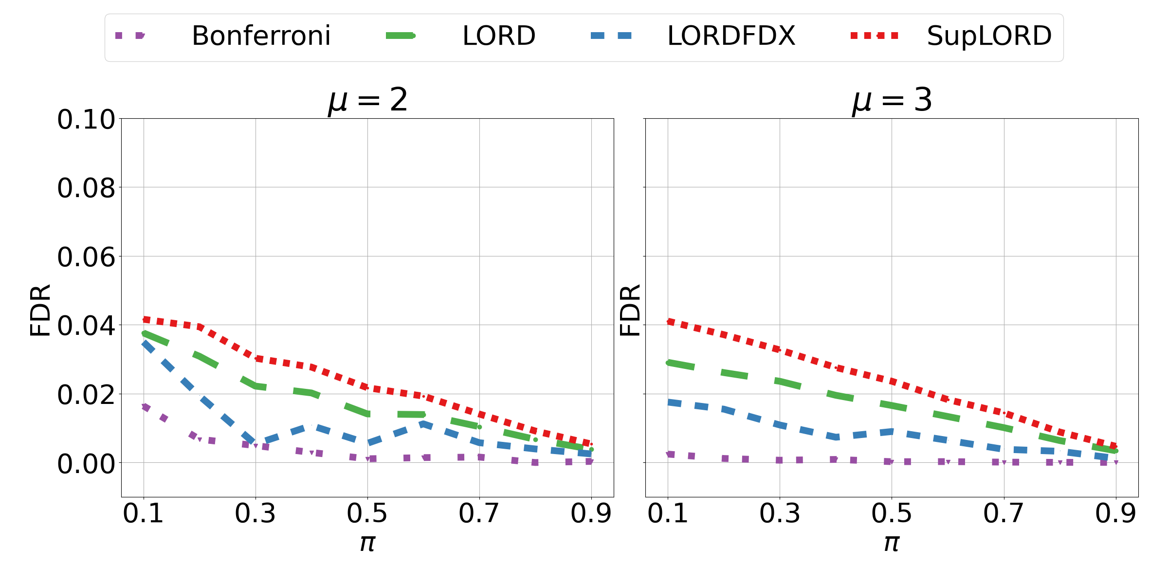
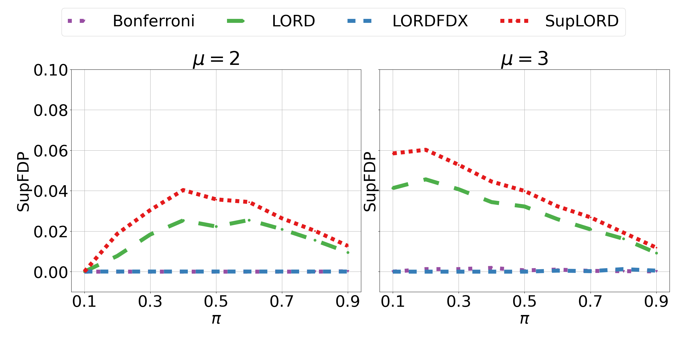
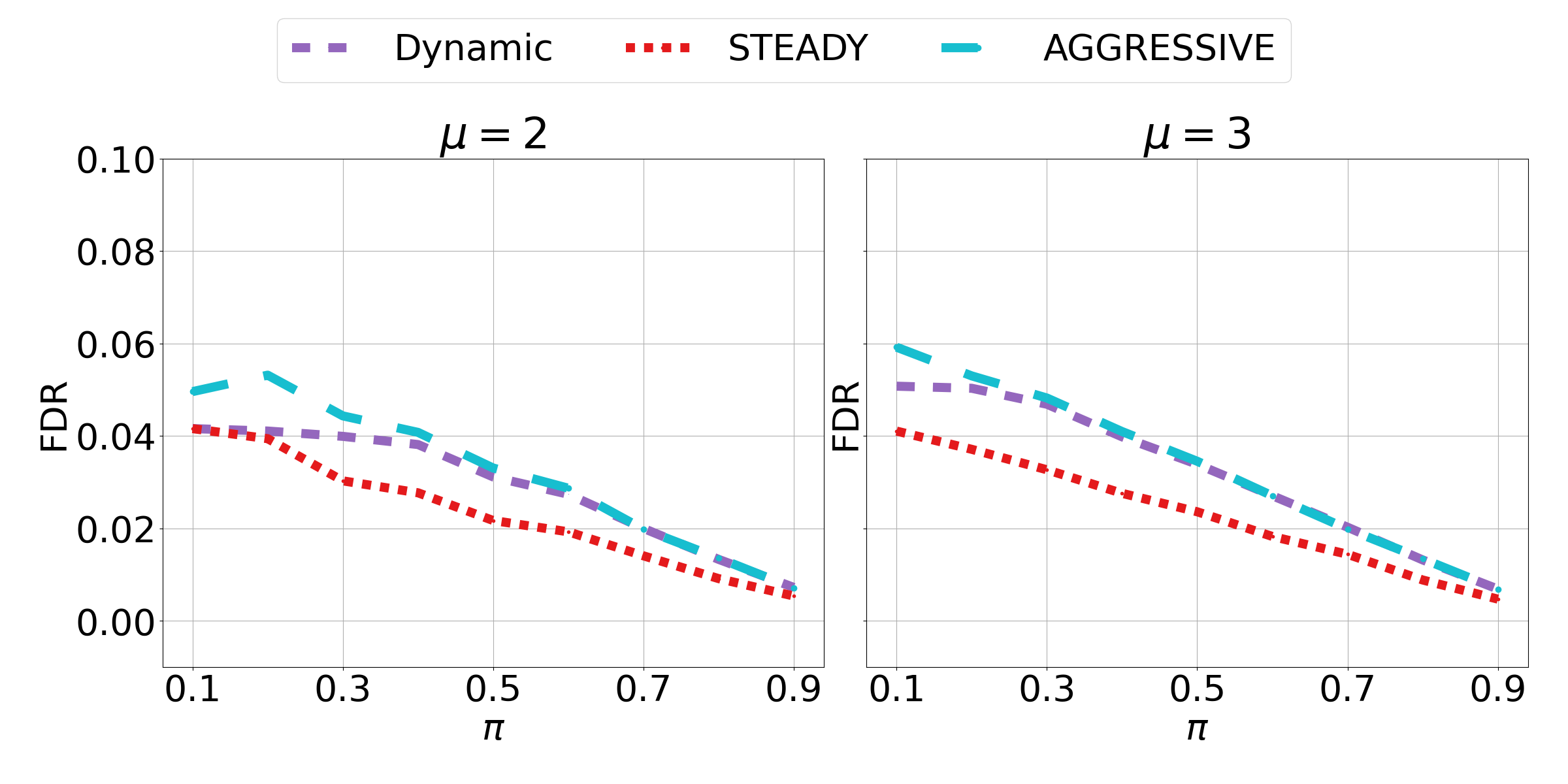
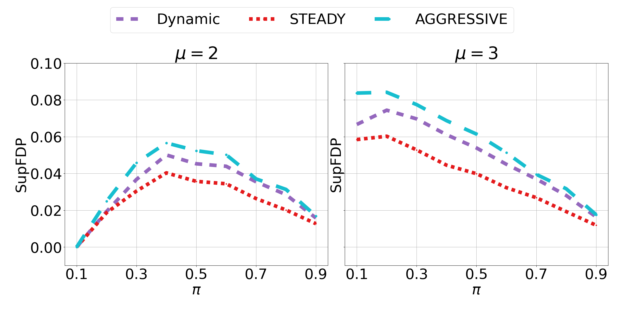
Refer to caption
Figure 6: Tradeoff between w0subscript𝑤0w_{0} and b𝑏b as a function of a𝑎a given δ=0.05,ϵ=0.15,r=20formulae-sequencesuperscript𝛿0.05formulae-sequencesuperscriptitalic-ϵ0.15superscript𝑟20\delta^{*}=0.05,\epsilon^{*}=0.15,r^{*}=20. Note that b𝑏b is increasing with respect to a𝑎a, while w0subscript𝑤0w_{0} has a maximum. We also denote the canonical triple as a triple (a,b,w0)𝑎𝑏subscript𝑤0(a,b,w_{0}), that can be selected to simultaneously maximize b𝑏b and w0subscript𝑤0w_{0}.

We illustrate in Figure 6 the relationship between a,b,𝑎𝑏a,b, and w0subscript𝑤0w_{0} for an example setting of ϵ=0.15,δ=0.05,formulae-sequencesuperscriptitalic-ϵ0.15superscript𝛿0.05\epsilon^{*}=0.15,\delta^{*}=0.05, and r=20superscript𝑟20r^{*}=20. We define the canonical triple for (a,b,w0)𝑎𝑏subscript𝑤0(a,b,w_{0}) as the b𝑏b and w0subscript𝑤0w_{0} corresponding to the a𝑎a that is the positive solution to problem (20). Note that for all a𝑎a smaller than the canonical a𝑎a, we may strictly improve any possible b𝑏b and w0subscript𝑤0w_{0} under that a𝑎a by selecting the canonical triple. On the other hand, the b𝑏b and w0subscript𝑤0w_{0} for any a𝑎a larger than the canonical a𝑎a form an optimal Pareto-frontier for trading off b𝑏b and w0subscript𝑤0w_{0}. Thus, the canonical a𝑎a can be treated as the default choice for a𝑎a and consequently, the user may avoid tuning additional hyperparameters. In addition, we may also define a default {βi}i{0}subscriptsubscript𝛽𝑖𝑖0\{\beta_{i}\}_{i\in\mathbb{N}\cup\{0\}} w.r.t. the canonical triple:

βi={1r(ϵrlog¯[a](1δ)a)itr1ϵlog¯[a](1δ)i>tr1.subscript𝛽𝑖cases1superscript𝑟superscriptitalic-ϵsuperscript𝑟subscript¯delimited-[]𝑎1superscript𝛿𝑎𝑖subscript𝑡superscript𝑟1superscriptitalic-ϵsubscript¯delimited-[]𝑎1superscript𝛿𝑖subscript𝑡superscript𝑟1\displaystyle\beta_{i}=\begin{cases}\frac{1}{r^{*}}\left(\frac{\epsilon^{*}r^{*}}{{\overline{\log}_{\left[a\right]}}{\left(\frac{1}{\delta^{*}}\right)}}-a\right)&i\leq t_{r^{*}-1}\\ \frac{\epsilon^{*}}{{\overline{\log}_{\left[a\right]}}{\left(\frac{1}{\delta^{*}}\right)}}&i>t_{r^{*}-1}.\end{cases} (21)

This default {βi}i{0}subscriptsubscript𝛽𝑖𝑖0\{\beta_{i}\}_{i\in\mathbb{N}\cup\{0\}} is tight with conditions (18) for the canonical a𝑎a, and can be considered as the default {βi}i{0}subscriptsubscript𝛽𝑖𝑖0\{\beta_{i}\}_{i\in\mathbb{N}\cup\{0\}} sequence for the general SupLORDSupLORD\mathrm{SupLORD} form.

Appendix B Proof of Theorem 2

First, we define the following term:

ca=01log¯[a](1δ)𝑑δ.subscript𝑐𝑎superscriptsubscript01subscript¯delimited-[]𝑎1𝛿differential-d𝛿\displaystyle c_{a}=\int\limits_{0}^{1}{\overline{\log}_{\left[a\right]}}{\left(\frac{1}{\delta}\right)}\ d\delta.

Note that the c𝑐c in Section 5 is defined with a=1𝑎1a=1, in which case c=c11.42𝑐subscript𝑐11.42c=c_{1}\leq 1.42.

Theorem 4.

Assuming conditional superuniformity (2), any GAI algorithm that satisfies conditions (18):

SupFDRtrcaϵlog¯(1δ).subscriptSupFDRsubscript𝑡superscript𝑟subscript𝑐𝑎superscriptitalic-ϵ¯1superscript𝛿\displaystyle\mathrm{SupFDR}_{t_{r^{*}}}~{}\leq~{}\frac{c_{a}\epsilon^{*}}{{\overline{\log}}{\left(\frac{1}{\delta^{*}}\right)}}.

Theorem 2 can be seen as an instance of this theorem where a=1𝑎1a=1.

To prove this theorem, we must prove a preliminary fact.

Fact 3 (Corollary 1 from an earlier revision of KR).

Let {αk}ksubscriptsubscript𝛼𝑘𝑘\{\alpha_{k}\}_{k\in\mathbb{N}} be any sequence of alpha values predictable with respect to filtration ksubscript𝑘\mathcal{F}_{k} in definition (1). Assume conditional superuniformity (2) is true, and let a>0𝑎0a>0 be fixed. Then, we obtain the following expected supremum ratio bound:

𝔼[supkFDP(k)FDP^a(k)]ca.𝔼delimited-[]subscriptsupremum𝑘FDPsubscript𝑘subscript^FDP𝑎subscript𝑘subscript𝑐𝑎\displaystyle\mathbb{E}\left[\sup_{k\in\mathbb{N}}\ \frac{\mathrm{FDP}(\mathcal{R}_{k})}{\widehat{\mathrm{FDP}}_{a}(\mathcal{R}_{k})}\right]\leq c_{a}.

We include a proof of this fact for completeness. First, we introduce another lemma from KR:

Fact 4 (Lemma 1 from KR).

Let the conditions of 3 be satisfied. Then, the following is true:

𝐏𝐫(supkFDP(k)FDP^a(k)>x)exp(aθxx),𝐏𝐫subscriptsupremum𝑘FDPsubscript𝑘subscript^FDP𝑎subscript𝑘𝑥𝑎subscript𝜃𝑥𝑥\displaystyle\mathbf{Pr}\left(\sup_{k\in\mathbb{N}}\ \frac{\mathrm{FDP}(\mathcal{R}_{k})}{\widehat{\mathrm{FDP}}_{a}(\mathcal{R}_{k})}>x\right)~{}\leq~{}\exp\left(-a\theta_{x}x\right),

where θxsubscript𝜃𝑥\theta_{x} is the unique solution to exp(θ)=1+θx𝜃1𝜃𝑥\exp(\theta)=1+\theta x.

Proof of 3.

First, we characterize x𝑥x when exp(aθxx)=δ𝑎subscript𝜃𝑥𝑥𝛿\exp(-a\theta_{x}x)=\delta in 4:

θxxsubscript𝜃𝑥𝑥\displaystyle\theta_{x}x =log(δ)a,absent𝛿𝑎\displaystyle=-\frac{\log(\delta)}{a},
θxsubscript𝜃𝑥\displaystyle\theta_{x} =log(log(δ)a+1).absent𝛿𝑎1\displaystyle=\log\left(-\frac{\log(\delta)}{a}+1\right). by exp(θx)=1+θxxsubscript𝜃𝑥1subscript𝜃𝑥𝑥\exp(\theta_{x})=1+\theta_{x}x

We now substitute this equality for θxsubscript𝜃𝑥\theta_{x} into the following:

exp(θx)subscript𝜃𝑥\displaystyle\exp(\theta_{x}) =1+θxx,absent1subscript𝜃𝑥𝑥\displaystyle=1+\theta_{x}x,
x𝑥\displaystyle x =exp(θx)1θxabsentsubscript𝜃𝑥1subscript𝜃𝑥\displaystyle=\frac{\exp(\theta_{x})-1}{\theta_{x}}
=log(δ)alog(log(δ)a+1)absent𝛿𝑎𝛿𝑎1\displaystyle=\frac{\frac{-\log(\delta)}{a}}{\log\left(-\frac{\log(\delta)}{a}+1\right)}
=log(1δ)alog(1+log(1δ)a)absent1𝛿𝑎11𝛿𝑎\displaystyle=\frac{\log\left(\frac{1}{\delta}\right)}{a\log\left(1+\frac{\log\left(\frac{1}{\delta}\right)}{a}\right)}
=log¯[a](1δ).absentsubscript¯delimited-[]𝑎1𝛿\displaystyle={\overline{\log}_{\left[a\right]}}{\left(\frac{1}{\delta}\right)}.

Now, we bound the expectation:

𝔼[supkFDP(k)FDP^a(k)]𝔼delimited-[]subscriptsupremum𝑘FDPsubscript𝑘subscript^FDP𝑎subscript𝑘\displaystyle\mathbb{E}\left[\sup_{k\in\mathbb{N}}\ \frac{\mathrm{FDP}(\mathcal{R}_{k})}{\widehat{\mathrm{FDP}}_{a}(\mathcal{R}_{k})}\right] =0𝐏𝐫(supknaturalsFDP(k)FDP^a(k)>x)𝑑xabsentsuperscriptsubscript0𝐏𝐫subscriptsupremum𝑘𝑛𝑎𝑡𝑢𝑟𝑎𝑙𝑠FDPsubscript𝑘subscript^FDP𝑎subscript𝑘𝑥differential-d𝑥\displaystyle=\int\limits_{0}^{\infty}\mathbf{Pr}\left(\sup_{k\in naturals}\ \frac{\mathrm{FDP}(\mathcal{R}_{k})}{\widehat{\mathrm{FDP}}_{a}(\mathcal{R}_{k})}>x\right)\ dx by quantile formula for expectation
0exp(aθxx)𝑑xabsentsuperscriptsubscript0𝑎subscript𝜃𝑥𝑥differential-d𝑥\displaystyle\leq\int\limits_{0}^{\infty}\exp(-a\theta_{x}x)\ dx by 4
=10δ𝑑log¯[a](1δ)absentsuperscriptsubscript10𝛿differential-dsubscript¯delimited-[]𝑎1𝛿\displaystyle=\int\limits_{1}^{0}\delta\ d{\overline{\log}_{\left[a\right]}}{\left(\frac{1}{\delta}\right)} substitute in δ𝛿\delta and exp(aθxx)𝑎subscript𝜃𝑥𝑥\exp(-a\theta_{x}x)
=0log¯[a](0)log¯[a](1)+01log¯[a](1δ)𝑑δ.absent0subscript¯delimited-[]𝑎0subscript¯delimited-[]𝑎1superscriptsubscript01subscript¯delimited-[]𝑎1𝛿differential-d𝛿\displaystyle=0\cdot{\overline{\log}_{\left[a\right]}}{\left(0\right)}-{\overline{\log}_{\left[a\right]}}{\left(1\right)}+\int\limits_{0}^{1}{\overline{\log}_{\left[a\right]}}{\left(\frac{1}{\delta}\right)}\ d\delta.

To simplify the last expression, we observe the following two facts:

limδ0+δlog¯[a](1δ)𝛿superscript0𝛿subscript¯delimited-[]𝑎1𝛿\displaystyle\underset{\delta\rightarrow 0^{+}}{\lim}\delta\cdot{\overline{\log}_{\left[a\right]}}{\left(\frac{1}{\delta}\right)}~{} =0,absent0\displaystyle=~{}0,
limδ1δlog¯[a](1δ)𝛿superscript1𝛿subscript¯delimited-[]𝑎1𝛿\displaystyle\underset{\delta\rightarrow 1^{-}}{\lim}\delta\cdot{\overline{\log}_{\left[a\right]}}{\left(\frac{1}{\delta}\right)}~{} =1.absent1\displaystyle=~{}1.

Thus, we can drop 0log¯[a](0)0subscript¯delimited-[]𝑎00\cdot{\overline{\log}_{\left[a\right]}}{\left(0\right)}, since it is 0, and 1log¯[a](1)1subscript¯delimited-[]𝑎1-1\cdot{\overline{\log}_{\left[a\right]}}{\left(1\right)} since it negative, and we achieve our desired upper bound. ∎

We proceed to prove Theorem 4.

SupFDRtrsubscriptSupFDRsubscript𝑡superscript𝑟\displaystyle\mathrm{SupFDR}_{t_{r^{*}}} =𝔼[supktrFDP(k)]absent𝔼delimited-[]𝑘subscript𝑡superscript𝑟supremumFDPsubscript𝑘\displaystyle=\mathbb{E}\left[\underset{k\geq t_{r^{*}}}{\sup}~{}\mathrm{FDP}(\mathcal{R}_{k})\right]
=𝔼[suprrFDP(tr)]absent𝔼delimited-[]𝑟superscript𝑟supremumFDPsubscriptsubscript𝑡𝑟\displaystyle=\mathbb{E}\left[\underset{r\geq r^{*}}{\sup}~{}\mathrm{FDP}(\mathcal{R}_{t_{r}})\right]
𝔼[suprrFDP(tr)FDP^a(tr)](suprrFDP^a(tr))absent𝔼delimited-[]𝑟superscript𝑟supremumFDPsubscriptsubscript𝑡𝑟subscript^FDP𝑎subscriptsubscript𝑡𝑟𝑟superscript𝑟supremumsubscript^FDP𝑎subscriptsubscript𝑡𝑟\displaystyle\leq\mathbb{E}\left[\underset{r\geq r^{*}}{\sup}~{}\frac{\mathrm{FDP}(\mathcal{R}_{t_{r}})}{\widehat{\mathrm{FDP}}_{a}(\mathcal{R}_{t_{r}})}\right]\cdot\left(\underset{r\geq r^{*}}{\sup}\ \widehat{\mathrm{FDP}}_{a}(\mathcal{R}_{t_{r}})\right) relaxation of supsupremum\sup
calog¯[a](1δ)(suprrFDP¯a(k))absentsubscript𝑐𝑎subscript¯delimited-[]𝑎1superscript𝛿𝑟superscript𝑟supremumsubscript¯FDP𝑎subscript𝑘\displaystyle\leq\frac{c_{a}}{{\overline{\log}_{\left[a\right]}}{\left(\frac{1}{\delta^{*}}\right)}}\cdot\left(\underset{r\geq r^{*}}{\sup}\ \overline{\mathrm{FDP}}_{a}(\mathcal{R}_{k})\right) by 3 and definition of FDP^a(k)subscript^FDP𝑎subscript𝑘\widehat{\mathrm{FDP}}_{a}(\mathcal{R}_{k})
caϵlog¯[a](1δ).absentsubscript𝑐𝑎superscriptitalic-ϵsubscript¯delimited-[]𝑎1superscript𝛿\displaystyle\leq\frac{c_{a}\epsilon^{*}}{{\overline{\log}_{\left[a\right]}}{\left(\frac{1}{\delta^{*}}\right)}}. by Lemma 2

Thus, we have shown that the general SupLORDSupLORD\mathrm{SupLORD} algorithm controls SupFDRSupFDR\mathrm{SupFDR} as claimed.

Appendix C Tighter Fixed Time FDRFDR\mathrm{FDR} Control

A tighter, fixed time FDRFDR\mathrm{FDR} bound exists for SupLORDSupLORD\mathrm{SupLORD} with additional constraints:

Theorem 5.

Assuming independent superuniformity (3), any GAI algorithm with a monotone spending schedule (5) that satisfies condition (18) and

β0+β1ϵlog¯[a](1δ),subscript𝛽0subscript𝛽1superscriptitalic-ϵsubscript¯delimited-[]𝑎1superscript𝛿\displaystyle\beta_{0}+\beta_{1}\leq\frac{\epsilon^{*}}{{\overline{\log}_{\left[a\right]}}{\left(\frac{1}{\delta^{*}}\right)}}, (22)

can ensure the following fixed time FDRFDR\mathrm{FDR} bound:

FDR1ϵlog¯[a](1δ).subscriptFDR1superscriptitalic-ϵsubscript¯delimited-[]𝑎1superscript𝛿\displaystyle\mathrm{FDR}_{1}~{}\leq~{}\frac{\epsilon^{*}}{{\overline{\log}_{\left[a\right]}}{\left(\frac{1}{\delta^{*}}\right)}}.

This result uses the same proof techniques as Ramdas et al. (2017, 2018); Tian and Ramdas (2019) for FDRFDR\mathrm{FDR} control, hence the much stronger assumptions and control only at fixed times. Thus, we can improve our FDRFDR\mathrm{FDR} control by a factor casubscript𝑐𝑎c_{a} of the cost of usability — independence is not necessarily a practical assumption, and control only at fixed times denies the flexibility of early stopping to the user.

Proof.

To prove Theorem 5, we utilize the following theorem from Ramdas et al. (2017):

Fact 5 (Theorem 1 from Ramdas et al. 2017).

Assuming independent superuniformity (3), any GAI algorithm with a monotone spending schedule eq. 5 with boost sequence {β}i{0}subscript𝛽𝑖0\{\beta\}_{i\in\mathbb{N}\cup\{0\}} controls FDRFDR\mathrm{FDR} at any fixed time:

FDR1max({β0+β1}{βi}i{0}).subscriptFDR1subscript𝛽0subscript𝛽1subscriptsubscript𝛽𝑖𝑖0\displaystyle\mathrm{FDR}_{1}\leq\max(\{\beta_{0}+\beta_{1}\}\cup\{\beta_{i}\}_{i\in\mathbb{N}\cup\{0\}}).

Thus, Theorem 5 follows directly from condition (24) and 5. ∎

An example specification for {βi}i{0}subscriptsubscript𝛽𝑖𝑖0\{\beta_{i}\}_{i\in\mathbb{N}\cup\{0\}} that satisfies the conditions of Theorem 5 is as follows:

βi={12r(ϵrlog¯[a](1δ)a)i=012r(ϵrlog¯[a](1δ)a𝐈{r>1})it11r(ϵrlog¯[1](1δ)a)t1<itr1ϵlog¯[1](1δ)i>tr1.subscript𝛽𝑖cases12superscript𝑟superscriptitalic-ϵsuperscript𝑟subscript¯delimited-[]𝑎1superscript𝛿𝑎𝑖012superscript𝑟superscriptitalic-ϵsuperscript𝑟subscript¯delimited-[]𝑎1superscript𝛿𝑎𝐈superscript𝑟1𝑖subscript𝑡11superscript𝑟superscriptitalic-ϵsuperscript𝑟subscript¯delimited-[]11superscript𝛿𝑎subscript𝑡1𝑖subscript𝑡superscript𝑟1superscriptitalic-ϵsubscript¯delimited-[]11superscript𝛿𝑖subscript𝑡superscript𝑟1\displaystyle\beta_{i}=\begin{cases}\frac{1}{2r^{*}}\left(\frac{\epsilon^{*}r^{*}}{{\overline{\log}_{\left[a\right]}}{\left(\frac{1}{\delta^{*}}\right)}}-a\right)&i=0\\ \frac{1}{2r^{*}}\left(\frac{\epsilon^{*}r^{*}}{{\overline{\log}_{\left[a\right]}}{\left(\frac{1}{\delta^{*}}\right)}}-a\cdot\mathbf{I}\left\{r^{*}>1\right\}\right)&i\leq t_{1}\\ \frac{1}{r^{*}}\left(\frac{\epsilon^{*}r^{*}}{{\overline{\log}_{\left[1\right]}}{\left(\frac{1}{\delta^{*}}\right)}}-a\right)&t_{1}<i\leq t_{r^{*}-1}\\ \frac{\epsilon^{*}}{{\overline{\log}_{\left[1\right]}}{\left(\frac{1}{\delta^{*}}\right)}}&i>t_{r^{*}-1}\end{cases}~{}~{}. (23)

We simply reduce β0+β1subscript𝛽0subscript𝛽1\beta_{0}+\beta_{1} such that they sum to at most the upper bound in condition (18b).

Appendix D mFDRmFDR\mathrm{mFDR} Control for SupLORDSupLORD\mathrm{SupLORD}

Fact 6 (Theorem 2 from Ramdas et al. 2017).

Let τ𝜏\tau be a stopping time. Assuming conditional superuniformity (2), any GAI algorithm with boost sequence {βi}i{0}subscriptsubscript𝛽𝑖𝑖0\{\beta_{i}\}_{i\in\mathbb{N}\cup\{0\}} ensures the following:

mFDR(τ)max({β0+β1}{βi}i{0}).mFDRsubscript𝜏subscript𝛽0subscript𝛽1subscriptsubscript𝛽𝑖𝑖0\displaystyle\mathrm{mFDR}(\mathcal{R}_{\tau})\leq\max(\{\beta_{0}+\beta_{1}\}\cup\{\beta_{i}\}_{i\in\mathbb{N}\cup\{0\}}).

Essentially, Ramdas et al. (2017) prove that the same algorithm can control FDRFDR\mathrm{FDR} at fixed times under p-variable independence and monotone scheduling, and mFDRmFDR\mathrm{mFDR} at stopping times under conditional superuniformity. Thus, we derive mFDRmFDR\mathrm{mFDR} control for SupLORDSupLORD\mathrm{SupLORD}:

Theorem 6.

Let τ𝜏\tau be a stopping time. Assuming conditional superuniformity (2), any GAI that satisfies condition (18) and

β0+β1ϵlog¯[a](1δ),subscript𝛽0subscript𝛽1superscriptitalic-ϵsubscript¯delimited-[]𝑎1superscript𝛿\displaystyle\beta_{0}+\beta_{1}\leq\frac{\epsilon^{*}}{{\overline{\log}_{\left[a\right]}}{\left(\frac{1}{\delta^{*}}\right)}}, (24)

can ensure the following fixed time FDRFDR\mathrm{FDR} bound:

mFDR(τ)ϵlog¯[a](1δ).mFDRsubscript𝜏superscriptitalic-ϵsubscript¯delimited-[]𝑎1superscript𝛿\displaystyle\mathrm{mFDR}(\mathcal{R}_{\tau})~{}\leq~{}\frac{\epsilon^{*}}{{\overline{\log}_{\left[a\right]}}{\left(\frac{1}{\delta^{*}}\right)}}.

Theorem 6 follows directly from conditions (18) and from 6. We can use the boost sequence in (23) as an example boost sequence that would give SupLORDSupLORD\mathrm{SupLORD} mFDRmFDR\mathrm{mFDR} control, since it also suffices for the assumptions in Theorem 6

Appendix E Additional Numerical Simulations

E.1 FDRFDR\mathrm{FDR} and SupFDRSupFDR\mathrm{SupFDR} in FDXFDX\mathrm{FDX} Control Simulations

Figure 7 shows that despite the nonexistent power LORDFDXLORDFDX\mathrm{LORD}\mathrm{FDX} possessed relative to SupLORDSupLORD\mathrm{SupLORD}, its error in FDRFDR\mathrm{FDR} is surprisingly close to SupLORDSupLORD\mathrm{SupLORD}. On other hand, LORDFDXLORDFDX\mathrm{LORD}\mathrm{FDX} has very low SupFDRSupFDR\mathrm{SupFDR} in Figure 8.

Refer to caption
Figure 7: Plot of non-null likelihood, π𝜋\pi, vs. FDRFDR\mathrm{FDR} for signal strengths of μ{2,3}𝜇23\mu\in\left\{2,3\right\} in the constant data setting. FDRFDR\mathrm{FDR} is controlled at =0.050.05\ell=0.05, and SupLORDSupLORD\mathrm{SupLORD} and LORDFDXLORDFDX\mathrm{LORD}\mathrm{FDX} are controlled at FDXFDX\mathrm{FDX} with ϵ=0.15superscriptitalic-ϵ0.15\epsilon^{*}=0.15 at a level of δ=0.05superscript𝛿0.05\delta^{*}=0.05. Experiment details in Section 3.2. SupLORDSupLORD\mathrm{SupLORD} has FDRFDR\mathrm{FDR} that is somewhat appropriate to its results in Theorem 5.
Refer to caption
Figure 8: Plot of non-null likelihood, π𝜋\pi, vs. SupFDR30subscriptSupFDR30\mathrm{SupFDR}_{30} for signal strengths of μ{2,3}𝜇23\mu\in\left\{2,3\right\} in the constant data setting. FDRFDR\mathrm{FDR} is controlled at =0.050.05\ell=0.05, and SupLORDSupLORD\mathrm{SupLORD} and LORDFDXLORDFDX\mathrm{LORD}\mathrm{FDX} are controlled at FDXFDX\mathrm{FDX} with ϵ=0.15superscriptitalic-ϵ0.15\epsilon^{*}=0.15 at a level of δ=0.05superscript𝛿0.05\delta^{*}=0.05. Experiment details in Section 3.2. SupLORDSupLORD\mathrm{SupLORD} has SupFDR30subscriptSupFDR30\mathrm{SupFDR}_{30} below what is expected by Theorem 2.
Refer to caption
Figure 9: Plot of non-null likelihood, π𝜋\pi, vs. FDRFDR\mathrm{FDR} for signal strengths of μ{2,3}𝜇23\mu\in\left\{2,3\right\} in the constant data setting. SupLORDSupLORD\mathrm{SupLORD} is controlled at FDXFDX\mathrm{FDX} with ϵ=0.15superscriptitalic-ϵ0.15\epsilon^{*}=0.15 at a level of δ=0.05superscript𝛿0.05\delta^{*}=0.05. Data details in Section 3.2, experiment details in Section 4.2. All schedules have similar FDRFDR\mathrm{FDR}.
Refer to caption
Figure 10: Plot of non-null likelihood, π𝜋\pi, vs. SupFDR30subscriptSupFDR30\mathrm{SupFDR}_{30} for signal strengths of μ{2,3}𝜇23\mu\in\left\{2,3\right\} in the constant data setting. FDRFDR\mathrm{FDR} is controlled at =0.050.05\ell=0.05, and SupLORDSupLORD\mathrm{SupLORD} and LORDFDXLORDFDX\mathrm{LORD}\mathrm{FDX} are controlled at FDXFDX\mathrm{FDX} with ϵ=0.15superscriptitalic-ϵ0.15\epsilon^{*}=0.15 at a level of δ=0.05superscript𝛿0.05\delta^{*}=0.05. Data details in Section 3.2, experiment details in Section 4.2. All schedules have similar SupFDRSupFDR\mathrm{SupFDR}.

E.2 Hidden Markov Model (HMM)

In addition to the standard Gaussian setting, we also perform simulations using a HMM process to model a setting where non-null where each hypothesis not independent of neighboring hypotheses. We set μi=μsubscript𝜇𝑖𝜇\mu_{i}=\mu to be constant for all i𝑖i, but we define πisubscript𝜋𝑖\pi_{i} as follows:

π1=0.5,πi={ξif Hi10,1ξif Hi10.formulae-sequencesubscript𝜋10.5subscript𝜋𝑖cases𝜉if subscript𝐻𝑖1subscript01𝜉if subscript𝐻𝑖1subscript0\displaystyle\pi_{1}=0.5,\quad\quad\pi_{i}=\begin{cases}\xi&\text{if }H_{i-1}\in\mathcal{H}_{0},\\ 1-\xi&\text{if }H_{i-1}\not\in\mathcal{H}_{0}.\end{cases}

If we let βisubscript𝛽𝑖\beta_{i} be the state at the i𝑖ith time step, we can view the data generating process as a two state HMM model with a ξ𝜉\xi probability of transitioning to the other state at the next time step. In expectation, there is an equal number of hypotheses that are null and non-null, regardless of the choice of ξ𝜉\xi. However, a smaller ξ𝜉\xi will result in large clusters of null or non-null hypotheses in consecutive time steps.

E.3 Results on HMM

We show extra results of the SupLORDSupLORD\mathrm{SupLORD} comparison with LORDLORD\mathrm{LORD} and LORDFDXLORDFDX\mathrm{LORD}\mathrm{FDX} on the HMM model in Figure 11.

\subfigureRefer to caption\subfigure

\subfigure

Figure 11: Plot of state transition probability, ξ𝜉\xi, vs. FDR, SupFDR30subscriptSupFDR30\mathrm{SupFDR}_{30}, and power where =0.050.05\ell=0.05 for signal strengths of μ{2,3}𝜇23\mu\in\left\{2,3\right\} in the HMM data setting. SupLORDSupLORD\mathrm{SupLORD} and LORDFDXLORDFDX\mathrm{LORD}\mathrm{FDX} are calibrated with δ=0.05superscript𝛿0.05\delta^{*}=0.05 for ϵ=0.15superscriptitalic-ϵ0.15\epsilon^{*}=0.15. We observe that SupLORDSupLORD\mathrm{SupLORD} has higher power across all ξ𝜉\xi and μ𝜇\mu, showing that it is not penalized by clustering of null or non-null hypotheses, relative to prior methods. (Recall that the definition of power only considers correctly rejected hypotheses. The gain in power is due to a less conservative algorithm that makes better use of its FDRFDR\mathrm{FDR}/FDXFDX\mathrm{FDX} budget.)
\subfigureRefer to caption\subfigure

\subfigure

Figure 12: Plot of the state change probability, ξ𝜉\xi, vs. FDRFDR\mathrm{FDR}, SupFDR30subscriptSupFDR30\mathrm{SupFDR}_{30}, and power in the HMM data setting comparing between SupLORDSupLORD\mathrm{SupLORD} with dynamic scheduling and without. The power plots suggests that dynamic scheduling is uniformly better than either steady or aggressive.

In Figure 12, we observe that in the HMM setting, dynamic scheduling remains the best choice, as it is superior or equal to the other schedules in power on all signal strengths and transition probabilities. In addition, if we compare the performance of dynamic scheduling and aggressive we note that the gap between the power of these two schedules is virtually nonexistent when the probability of changing states, ξ𝜉\xi, is low. The exact reverse is true when comparing dynamic scheduling and steady — they have similar power when ξ𝜉\xi is high. This reflects the ability of dynamic scheduling to adapt to the distribution of non-null hypotheses by dynamically adjusting its behavior in accordance with the wealth of the algorithm. Consequently, it incorporates the strengths of both steady and aggressive, and is more powerful regardless of ξ𝜉\xi as a result.

Appendix F Illustrating the Dynamic Scheduling Improvement

To illustrate the difference between dynamic scheduling and baseline static schedules, we plot the different alpha values produced by each scheduling algorithm with SupLORDSupLORD\mathrm{SupLORD} for a single trial. In Figure 13, we plot the difference between alpha values of dynamic scheduling and each of the baseline schedules for a single trial in the constant data setting, where non-null frequency is π=0.3𝜋0.3\pi=0.3 and non-null mean is μ=3𝜇3\mu=3. We see that for the majority of hypotheses, dynamic scheduling outputs αisubscript𝛼𝑖\alpha_{i} that are larger by about 0.005. Note that a dynamic schedule only makes more rejections if the p-value lies in the gap between the alpha value output by the baseline schedule, and the alpha value output by the dynamic schedule. Further, a p-value from a non-null hypothesis generally lies in this alpha value gap with slightly higher probability than a uniform distribution for the null hypothesis e.g. it may be within the gap with 0.01–0.02 probability. Thus, dynamic scheduling gets consistent power gains over each of the baselines by having generally larger alpha values than baseline schedules.

\subfigure

[Dynamic α𝛼\alphasteady α𝛼\alpha] Refer to caption

\subfigure

[Dynamic α𝛼\alphaaggressive α𝛼\alpha] Refer to caption

Figure 13: Plot of differences in alpha values between dynamic scheduling and each baseline static schedule for an identical trial of p-values generated by the same seed in the constant data setting with non-null frequency π=0.3𝜋0.3\pi=0.3, and non-null mean μ=3𝜇3\mu=3. Green bars mark steps where dynamic scheduling has higher alpha value, and red marks steps where the baseline static schedule has a higher alpha value. Dynamic scheduling has higher alpha values by about 0.005 for the majority of the trial when compared to both baseline schedules.

We plot the actual alpha values for each schedule of the single run in Figure 14 and the mean alpha values of each schedule across 200 runs in Figure 15. In Figure 15, we can observe that dynamic scheduling has consistently larger alpha values than both schedules, albeit by a small amount.
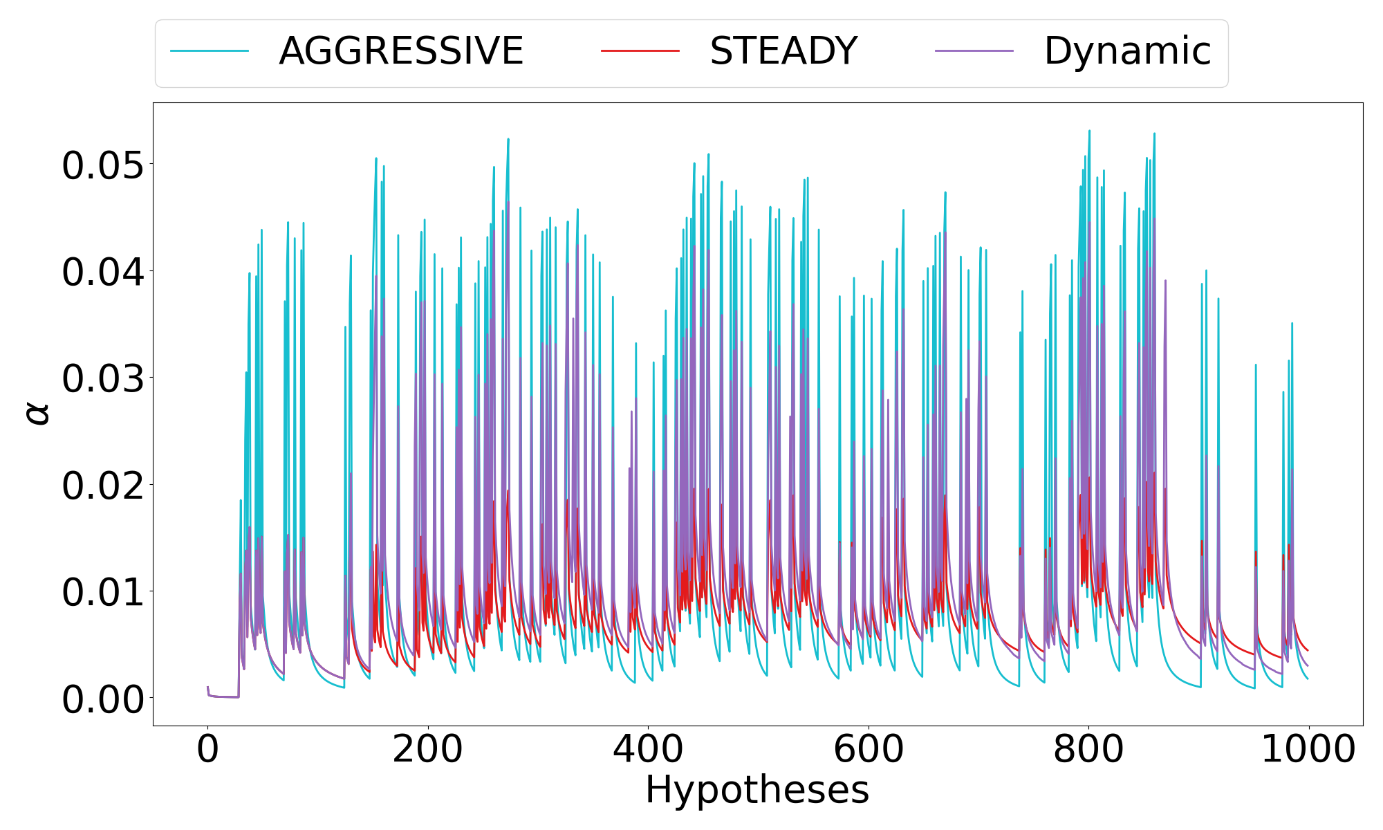
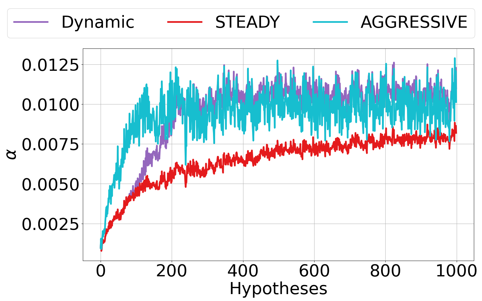
Refer to caption
Figure 14: (Raw values) Plot of actual alpha values between dynamic scheduling and each baseline static schedule for an identical trial of p-values generated by the same seed in the constant data setting with non-null frequency π=0.3𝜋0.3\pi=0.3, and non-null mean μ=3𝜇3\mu=3.
Refer to caption
Figure 15: (Mean values) Plot of mean alpha values between dynamic scheduling and each baseline static schedule in the constant data setting with non-null frequency π=0.3𝜋0.3\pi=0.3, and non-null mean μ=3𝜇3\mu=3 over 200 trials. We can observe that dynamic scheduling is generally larger than both baseline schedules by a small amount in a consistent fashion.