A measurement-based variational quantum eigensolver

Abstract

Variational quantum eigensolvers (VQEs) combine classical optimization with efficient cost function evaluations on quantum computers. We propose a new approach to VQEs using the principles of measurement-based quantum computation. This strategy uses entangled resource states and local measurements. We present two measurement-based VQE schemes. The first introduces a new approach for constructing variational families. The second provides a translation of circuit-based to measurement-based schemes. Both schemes offer problem-specific advantages in terms of the required resources and coherence times.

Variational methods are crucial to investigate the physics of strongly correlated quantum systems. Numerical tools like the density matrix renormalization group Perez-Garcia et al. (2007); Haegeman et al. (2013); Orús (2014); Evenbly and Vidal (2015) have been applied to several problems including real-time dynamics Güttge et al. (2013), condensed matter physics He et al. (2017), lattice gauge theories Banuls et al. (2014); Bañuls and Cichy (2020); Dalmonte and Montangero (2016); Bender et al. (2020), and quantum chemistry Chan et al. (2008); Krumnow et al. (2016). Nevertheless, the classes of states that can be studied with classical computers is limited Ortiz et al. (2001). Variational quantum eigensolvers (VQEs) overcome this problem using a closed feedback loop between a classical computer and a quantum processor McClean et al. (2016); Farhi et al. (2014); Preskill (2018). The classical algorithm optimizes a cost function – typically the expectation value of some operator – which is efficiently supplied by the quantum hardware. The VQE provides an approximation to the (low-lying) eigenvalues of this operator and the corresponding eigenstates. VQEs are advantageous for a variety of applications Shehab et al. (2019a); Preskill (2018); Bañuls et al. (2020); Kaubruegger et al. (2019); Dumitrescu et al. (2018); Haase et al. (2020); Bauer et al. (2016) and have been experimentally demonstrated in fields including chemistry McArdle et al. (2020); O’Malley et al. (2016), particle physics Kokail et al. (2019); Paulson et al. (2020); Shehab et al. (2019b); Lu et al. (2019), and classical optimization Borle et al. (2020); Bravo-Prieto et al. (2020); Kyriienko et al. (2020).

Existing VQE protocols are based on the circuit model, where gates are applied on an initial state Peruzzo et al. (2014). These gates involve variational parameters whose optimization allows the resulting output state to approximate the desired target state. We propose a new approach to VQE protocols, based on the measurement-based model of quantum computation (MBQC) Raussendorf and Briegel (2001); Briegel et al. (2009); Browne and Briegel (2006); Raussendorf et al. (2003); Walther et al. (2005); Larsen et al. (2020). In MBQC, an entangled state is prepared and the computation is realized by performing single-qubit measurements. While the circuit-based and measurement-based models both allow for universal quantum computation and have equivalent scaling of resources Raussendorf et al. (2003), they are intrinsically different. The former is limited by the number of available qubits and gates that can be performed, and MBQC by the size of the entangled state one can generate. For certain applications, the required coherence times Zwerger et al. (2015, 2014) and error thresholds Raussendorf et al. (2003); Zwerger et al. (2015, 2013, 2014) are much less demanding for MBQC.

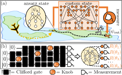
Figure 1: MB-VQE schemes. (a) Variation of a problem-specific ansatz state by ‘edge decoration’. An ansatz graph state starts the MB-VQE in a suitable corner of Hilbert space (choice of green island). Next, a classical algorithm explores the neighbourhood (runner on black arrow). The variational optimization exploits a custom state that is obtained by decorating the edges of the ansatz state with auxiliary qubits (orange circles). Their measurement in rotated bases $R(\theta)$ with variational parameters $\theta$ transforms $\lvert\psi_{\rm a}\rangle$ into the output state $\lvert\psi_{\rm out}\rangle$. (b) Direct translation of a VQE circuit into a MB-VQE. Left: circuit consisting of Clifford gates (black) and single-qubit parametric gates (‘knobs’). Right: corresponding MB-VQE, where the Clifford-part of the circuit has been performed beforehand. The custom state consists of output (white circles) and auxiliary (orange circles) qubits only; the latter are measured in rotated bases and are related to the ‘knobs’ in the circuit.

Here, we develop a new variational technique based on MBQC, that we call measurement-based VQE (MB-VQE). Our protocols determine the ground state of a target Hamiltonian, which is a prototypical task for VQEs with wide-ranging applications McClean et al. (2016); McArdle et al. (2020); Dumitrescu et al. (2018); Bauer et al. (2016); Moll et al. (2018); Paulson et al. (2020); Haase et al. (2020). The underlying idea is to use a tailored entangled state called ‘custom state’, that allows for exploring an appropriate corner of the system’s Hilbert space [Fig. 1(a)]. This custom state includes auxiliary qubits which, once measured, modify the state of the output qubits. The choices of the measurement bases, and the corresponding variational changes to the state, are controlled by a classical optimization algorithm. This approach differs conceptually and practically from standard VQE schemes since MB-VQE shifts the challenge from performing multi-qubit gates to creating an entangled initial state.

After presenting the framework for the MB-VQE, we design two specific schemes that are suited to different problem classes. First, we introduce a novel method to construct variational state families, illustrated using the toric code model with local perturbations Hübener et al. (2011). As Fig. 1(a) shows, we start from an ansatz state $\lvert\psi_{\rm a}\rangle$ in an appropriate corner of the Hilbert space. To explore this neighbourhood using a classical optimization algorithm, we introduce a custom state and apply measurement-based modifications of $\lvert\psi_{\rm a}\rangle$ that have no direct analogue in the circuit-model. The resulting variational family is not efficiently accessible with known classical methods and is more costly to access with circuit-based VQEs.

Second, we introduce a direct translation of circuit VQEs to MB-VQEs [Fig. 1(b)]. Here, the variational state family is the same for the circuit- and the measurement-based approaches, but the implementation differs as the MB-VQE requires different resources and is manipulated by single-qubit measurements only. We exemplify this direct translation for the Schwinger model Schwinger (1951) and highlight the different hardware requirements and the scaling of resources. As explained below, a translation to MB-VQE is advantageous for circuits containing a large fraction of so-called Clifford gates (e.g. $CX$ gates), as these are absorbed into the custom state.

While MB-VQE is platform agnostic, it opens the door for complex quantum computations in systems where long gate sequences or the realization of entangling gates are challenging. In particular, MB-VQE offers new routes for experiments with photonic quantum systems, thus enlarging the toolbox of variational computations.

General framework The main resource of MBQC are so-called graph states Hein et al. (2004, 2006). Graphs as in Fig. 1 are stabilizer states (eigenstates with $+1$ eigenvalues) of the operators $\hat{S}_{n}=\hat{X}_{n}\prod_{k}\hat{Z}_{k}$, where $k$ refers to the vertices connected to site $n$. To obtain the desired final state encoded in the output qubits (white circles), single-qubit measurements are performed on auxiliary qubits (orange circles), either in the eigenbasis of the Pauli operators $\hat{X}$, $\hat{Y}$, $\hat{Z}$, or in the rotated basis $R(\theta)\equiv\{(|{0}\rangle\pm e^{i\theta}|{1}\rangle)/\sqrt{2}\}$. Depending on the measurement outcomes, the system is probabilistically projected into different states. To make the computation deterministic, so-called byproduct operators and adaptive measurements are required Raussendorf et al. (2003). The former applies $\hat{X}$ and $\hat{Z}$ operators to the output qubits depending on the measurement results, while the latter involves adapting the measurement bases $R(\theta)$ based on earlier measurement outcomes. Consequently, adaptive measurements must be performed in a specific order.

An advantage of MBQC is the possibility to simultaneously perform all non-adaptive measurements at the beginning of the calculation (see Fig. 1(b) and Supplemental Material (SM) sup ). This corresponds to the Clifford part of a circuit and includes single- and many-qubit gates. This is independent of the position of the gates in the circuit, and reduces the required overhead and coherence time. Remarkably, this can be either done directly on the graph state in the quantum hardware, or on a classical computer before the experiment. In the latter case, the Gottesmann-Knill theorem Aaronson and Gottesman (2004) allows for efficiently determining the custom state which is local-Clifford equivalent to the quantum state obtained after all non-adaptive measurements are performed Van den Nest et al. (2004). This state can be directly prepared and used for the MBQC, which may have dramatically fewer auxiliary qubits compared to the initial graph state.

We now explain how MBQC is used to design a MB-VQE. While the classical part of the feedback loop is untouched (the best optimization algorithm Kingma and Ba (2014); Ruder (2017); Stokes et al. ; Audet and Dennis ; Rasmussen (2003); Frazier (2018) is problem dependent Paulson et al. (2020); Cerezo et al. (2020)), the MB-VQE is based on the creation and partial measurement of a tailored graph state rather than the application of a sequence of gates. Specifically, the quantum part of a MB-VQE comprises an ansatz state $\lvert\psi_{\rm a}\rangle$, a custom state, and a measurement prescription. As schematically represented in Fig. 1(a), $\lvert\psi_{\rm a}\rangle$ is a graph state from which we start exploring the variational class of families attainable by the MB-VQE. The custom state is then created by expanding $\lvert\psi_{\rm a}\rangle$ into a bigger graph state. This is done by decoration, i.e. by adding new vertices and connecting them to pre-existing sites in the ansatz state. According to a measurement prescription, which is the same at each iteration of the algorithm, the auxiliary qubits of the custom state are then measured, with the remaining ones constituting the output $\lvert\psi_{\rm out}\rangle$ of the quantum processor [see Fig. 1(a)]. The cost function to be fed into the classical side of the MB-VQE is then calculated from $\lvert\psi_{\rm out}\rangle$ (e.g. its energy), with the angles $\theta$ of the rotated bases $R(\theta)$ being the variational parameters over which the optimization occurs.

Just like the circuit in a VQE, the custom state determines the success of our MB-VQE. Generally, the more auxiliary qubits are measured in rotated bases $R(\theta)$, the bigger the available class of variational states that can be explored. However, an excessive number of parameters $\theta$ makes the algorithm’s convergence slower. Therefore, it is convenient to tailor the custom state to the considered problem. And qubit decoration, with the subsequent measurement of the auxiliary qubits, allows for remarkable control over the desired ansatz state’s transformation(s). Not only can one apply gates – just like in a circuit-based VQE – by following MBQC prescriptions (see the Schwinger model example), one can also identify completely new patterns of auxiliary qubits, that modify the output state in a way that would be expensive or even impossible with the circuit formalism (see the toric code example). For instance, a single auxiliary qubit measured in $R(\theta)$ and connected to an arbitrary number of output qubits $\{1,2,3,\dots\}$, acts $e^{i\frac{\theta}{2}\hat{Z}_{1}\otimes\hat{Z}_{2}\otimes\hat{Z}_{3}\otimes\dots}$ onto them Browne and Briegel (2006). In a circuit, the same operation requires a linear number of two-qubit gates .

State variation by edge-modification (perturbed toric code) Here, we demonstrate how a MB-VQE manipulates states in a different way than a circuit-based VQE. MB-VQEs are advantageous whenever a perturbation $\hat{H}_{\rm p}$ is added to a Hamiltonian $\hat{H}_{0}$ whose ground state, used as ansatz state $\lvert\psi_{\rm a}\rangle$ below, is a stabilizer state or a graph state.

To create the custom state from $\lvert\psi_{\rm a}\rangle$ we employ the pattern in Fig. 2(a), that decorates each connected pair of output qubits $m$ and $n$ with four auxiliary qubits $(m,n)_{i}$ ($i=1,\dots,4$), to be measured in rotated bases $R(\theta)$. Depending on $R(\theta)$, the entanglement between the qubits $m$ and $n$ is modified, and their state subjected to an additional rotation. For example, if all auxiliary qubits in the custom state are measured with $\theta=0$, we obtain the original ansatz state. However, if all auxiliary qubits are measured with $\theta=\pi/2$, then all entanglement of $\lvert\psi_{\rm a}\rangle$ is eliminated (for more details, see SM sup ). This decoration technique is tailored to the perturbed toric code example below, in which the ground states of $\hat{H}_{\rm 0}$ and $\hat{H}_{\rm p}$ are maximally entangled and pure, respectively. However, it can be easily generalized to expand the class of available variational states (see SM sup ), thus suiting different scenarios.

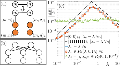
Figure 2: Perturbed toric code. (a) Edge modification resource for the MB-VQE [see Fig. 1(a)]. Four auxiliary qubits (orange circles), labelled $(m,n)_{i}$ ($i=1,\dots,4$), are added to two connected output qubits $m$ and $n$ (white circles). (b) Graph state representation of the ansatz state $\lvert 0,0\rangle_{L}$. Additional Hadamard gates are applied to qubits with dashed lines. (c) Relative difference between the MB-VQE result and the true ground state energy vs the perturbation strength. We let $\lambda_{n}$ in Eq. (1) be equal on all qubits (solid blue line), or sampled from a normal distribution $P_{G}$ of average $\lambda$ and variance $0.1\lambda$ (red squares). Green triangles describe a perturbation acting strongly on $\lambda_{1}$ and weakly on the other qubits. Dotted and dashed lines are computed with respect to $\lvert 0,0\rangle_{L}$ (ansatz state) and $\lvert 1\rangle^{\bigotimes 2N_{x}N_{y}}$ (ground state of $\hat{H}_{\rm p}$) for $\lambda_{n}=\lambda$ $\forall n$.

We apply this MB-VQE approach to the toric code model, a quantum error-correcting code defined on a two-dimensional rectangular lattice with periodic boundary conditions Kitaev (2003). On the lattice, the number of rows (columns) of independent vertices is $N_{x}$ ($N_{y}$) and edges represent qubits. The toric code state is a stabilizer state of so-called star $\hat{A}_{s}$ and plaquette $\hat{B}_{p}$ operators. For any vertex $s$ in the lattice, $\hat{A}_{s}$ acts $\hat{Z}$ on the four incident edges, while $\hat{B}_{p}$ acts $\hat{X}$ on the four edges in the $p$-th plaquette. The toric code Hamiltonian is then $\hat{H}_{0}=-\sum_{s}\hat{A}_{s}-\sum_{p}\hat{B}_{p}$. Since $\prod_{s}\hat{A}_{s}=\prod_{p}\hat{B}_{p}=1$, the toric code has $2N_{x}N_{y}-2$ independent stabilizers, and $\hat{H}_{0}$ has four degenerate ground states $|{r,t}\rangle_{L}$ ($r,t=0,1$), called logical states below. These are simultaneous eigenstates of $\hat{H}_{0}$ and the two logical-$Z$ operators Kitaev (2003), as explained in the SM sup .

The perturbation added to the toric code Hamiltonian is

$$\hat{H}_{\rm p}=\sum_{n=1}^{2N_{x}N_{y}}\lambda_{n}\hat{Z}_{n},$$ (1)

which corresponds to an inhomogeneous magnetic field. As ansatz state for the MB-VQE we choose the highly entangled graph state $|{\psi_{\rm a}}\rangle=|{0,0}\rangle_{L}$, that approximates the ground state of $\hat{H}_{0}+\hat{H}_{\rm p}$ for small positive values of $\lambda_{n}$. The graph state representation of $|{0,0}\rangle_{L}$ can be calculated efficiently classically Van den Nest et al. (2004) and is shown in Fig. 2(b) for $N_{x}=N_{y}=2$. In SM sup , we explain how to adapt our MB-VQE protocol to use an arbitrary superposition of $|{r,t}\rangle_{L}$ ($r,t=0,1$) as ansatz state, which is more suited for different kinds of perturbations $\hat{H}_{\rm p}$.

Numerical results for the MB-VQE are shown in Fig. 2(c). The relative energy difference between the MB-VQE result and the true ground state (calculated via exact diagonalization) is plotted against the perturbation strength. This is done with all $\lambda_{n}$ in Eq. (1) equal to $\lambda$ (solid blue line), with each $\lambda_{n}$ drawn from a Gaussian distribution $P_{G}(\mu,\sigma^{2})$ with mean $\mu=\lambda$ and variance $\sigma^{2}=0.1\lambda$ (orange squares), and with $\lambda_{1}=\lambda$, $\lambda_{n}$ randomly sampled from $P_{G}(\mu=0.1,\sigma^{2}=10^{-4})$ for $n\neq 1$ (green triangles). A plot of the infidelity resembles Fig. 2(c), with maximum infidelities for the blue curve, red squares and green triangles being 6.2$\times 10^{-2}$, 6.5$\times 10^{-2}$, and 9.4$\times 10^{-3}$, respectively. Fig. 2(c) shows that the MB-VQE produces the ground state energy with high confidence when the perturbation strength is very small or very large. Notably, the MB-VQE outperforms the ansatz state (dotted black line) and the ground state of $\hat{H}_{\rm p}$ in Eq. (1) (dashed black line) in all cases. If the perturbation only acts on one qubit, the chosen custom state allows the MB-VQE to find the exact ground state energy within machine precision. This is also the case if the perturbation acts on two disconnected qubits, provided we connect them and add auxiliary qubits as in Fig. 2(a). This suggests that the outcome of the MB-VQE can be significantly improved by adding few extra auxiliary qubits.

Translating VQEs into MB-VQEs (Schwinger model) Instead of the approach described above, one can create a MB-VQE by translating the circuit of a VQE into its corresponding custom state and a sequence of measurements. Since a universal set of gates can be realized in a MBQC Raussendorf et al. (2003), any VQE can be translated into a MB-VQE. As we discuss below, this strategy is advantageous if the number of parametric adaptive measurements [i.e. ‘knobs’ in Fig. 1(b)] in the resulting MB-VQE scheme is small.

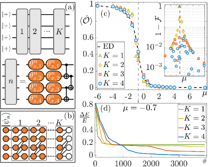
Figure 3: Schwinger model. (a) Ansatz state and VQE circuit for $S=4$ qubits and $K$ layers. Each layer consists of $CX$ gates and local rotations (orange) parametrized by angles $\theta_{\nu,i}^{n}$ (with rotation axis $\nu=x,z$; $i=1,\dots,4$). (b) MB-VQE custom state for $K$ layers. White circles are output qubits. Auxiliary qubits (orange) are measured in a rotated bases $R(\theta)$. (c) The order parameter $\langle{\hat{\mathcal{O}}}\rangle$ vs the fermion mass $\mu$. The dashed line and dots represent exact diagonalization ($ED$) and (MB-)VQE results, respectively, with the number of layers $K$ indicated in the legend. The inset shows the infidelity $1-\mathcal{F}$. (d) Relative energy difference $\Delta E/E$ between (MB-)VQE results and $ED$ for $\mu=-0.7$, versus the number of iterations in the optimization procedure. The variational parameters are initialized at zero, and $J=\omega=1$ in Eq. (2).

As an example, we determine the ground state energy of the Schwinger model Schwinger (1951), a testbed used for benchmarking quantum simulations in high energy physics Kokail et al. (2019); Klco et al. (2018); Bañuls and Cichy (2020). The Schwinger model describes quantum electrodynamics on a one-dimensional lattice and can be cast in the form of a spin model with long range interactions Hamer et al. (1997); Martinez et al. (2016); Muschik et al. (2017),

$$\begin{split}\hat{H}&=\frac{J}{2}\sum_{n=1}^{S-2}\sum_{k=n+1}^{S-1}(S-k)\hat{Z}_{n}\hat{Z}_{k}-\frac{J}{2}\sum_{n=1}^{S-1}n\text{mod}2\sum_{k=1}^{n}\hat{Z}_{k}\\ &+w\sum_{n=1}^{S-1}\left(\hat{\sigma}_{n}^{+}\hat{\sigma}_{n+1}^{-}+\text{H.C.}\right)+\frac{\mu}{2}\sum_{n=1}^{S}(-1)^{n}\hat{Z}_{n},\end{split}$$ (2)

where $S$ is the number of fermions, $\mu$ their mass, $w=\frac{1}{2a}$, and $J=\frac{g^{2}a}{2}$. Here, $a$ and $g$ are the lattice spacing and the coupling strength, respectively, and $\hat{\sigma}^{\pm}_{n}=(\hat{X}_{n}\pm i\hat{Y}_{n})/2$.

For the VQE protocol, we assume the typical situation where parametric single-qubit gates and fixed entangling gates ($CX$s) are used Arute et al. (2020); McArdle et al. (2020). We consider a generic VQE circuit, in which a sequence of ‘layers’ is applied McClean et al. (2016), each containing local rotations and entangling gates. As shown in Fig. 3(a) for $S=4$, we choose the layer

$$\prod_{n=1}^{S/2-1}CX_{2n,2n+1}\prod_{n=1}^{S/2}CX_{2n-1,2n}\prod_{n=1}^{S}\hat{U}_{x,n}(\theta_{x,n})\hat{U}_{z,n}(\theta_{z,n}),$$ (3)

where $\hat{U}_{\nu,n}(\theta_{\nu,n})=\exp{(i\theta_{\nu,n}\hat{V}_{n}/2)}$ [$(\nu,\hat{V})=(x,\hat{X})$ or $(\nu,\hat{V})=(z,\hat{Z})$]. The circuit for the VQE is created by concatenating $K$ layers, where $K$ is big enough to sufficiently explore the relevant subsector of the considered Hilbert space. As described in the SM sup , the MB-VQE custom state corresponding to a $K$-layer circuit is obtained by joining the measurement patterns of the gates in Eq. (3), and performing all non-adaptive measurements classically, which effectively removes the Clifford parts of the circuit. The custom state is shown in Fig. 3(b). As ansatz state we use $|\psi_{\rm a}\rangle=\bigotimes_{n=1}^{S}\lvert+\rangle$.

The (MB-)VQE simulation results are shown in Fig. 3(c) for $S=4$ and different values of $K$. We plot the order parameter $\langle{\hat{\mathcal{O}}}\rangle=\frac{1}{2S(S-1)}\sum_{i,j<i}\langle{(1+(-1)^{i}\hat{Z}_{i})(1+(-1)^{j}\hat{Z}_{j})}\rangle$ against the fermion mass $\mu$ and correctly observe a second-order phase transition around $\mu=-0.7$ Coleman (1976); Kokail et al. (2019); Yang et al. (2016). Increasing $K$ improves the ground state approximation, as demonstrated by the inset in Fig. 3(c) and by Fig. 3(d). The points near the phase transition require $K\gtrsim 3$ layers ($\gtrsim 28$ qubits), whereas $K=1$ layer ($12$ qubits) suffices for the easiest points. Note that allowing different gates as resources in Eq. (3) generally leads to different convergence rates, as demonstrated by the results in Ref. Kokail et al. (2019).

Perfect platforms provided, both the VQE and the MB-VQE give the same result. However, the quantum hardware requirements are different for the two methods. The circuit-based VQE requires $S$ qubits, $2KS$ single-qubit operations, and $K(S-1)$ entangling gates. For the corresponding MB-VQE, a custom state of $S(2K+1)$ qubits and $2KS$ single-qubit operations (measurements) are required. Generally, translating a VQE into its corresponding MB-VQE is advantageous whenever the VQE circuit involves a large Clifford part compared to the number of adaptive measurements (i.e. knobs). In this case, MB-VQE avoids the requirement of performing long gate sequences, which is currently challenging due to error accumulation. This is especially interesting for platforms where entangling gates are hard to realize (e.g. photonic setups) or in systems with limited coherence times.

Conclusions In this paper, we merged the principles of measurement-based quantum computation and quantum-classical optimization to create a MB-VQE. We presented two new types of variational schemes, that are not restricted to our specific examples and can be combined. The first applies when the ansatz state is a stabilizer state. In this case, it is classically efficient to determine the corresponding graph state Van den Nest et al. (2004), which is decorated with additional control qubits and prepared directly. We applied this MB-VQE to the perturbed toric code. Additionally, we showed how to adapt any circuit-based VQE to become a MB-VQE, with the Schwinger model as example.

Experimental proof-of-concept demonstrations can be explored by considering the smallest instance of the planar code Kitaev (2003) with a perturbation on a single qubit as first step. In this scenario, the MB-VQE requires as few as eight entangled qubits instead of the $44$ used above. Especially promising candidate systems include superconducting qubits, and photonic platforms. The latter recently demonstrated the capability to entangle several thousands of qubits Asavanant et al. (2019); Larsen et al. (2019), and to create tailored graph states Tiurev et al. (2020a, b); Schwartz et al. (2016); Bastin et al. (2009). When designing custom states for future experiments, it will be important to understand the effects of decoherence and it will be interesting to investigate whether MB-VQEs retain the high robustness of MBQC against errors Zwerger et al. (2015, 2013, 2014).

Our scheme based on edge decoration provides a new way of thinking about state variations in VQEs. In particular, the effects resulting from measuring only one or few entangled auxiliary qubits can be challenging to describe with a simple circuit. The resulting state modifications do not necessarily correspond to unitary operations and can affect a large number of remaining qubits Browne and Briegel (2006). Accordingly, MB-VQEs can lead to schemes in which few auxiliary qubits suffice to reach the desired state, while many gates would be required in a circuit-based protocol. Just like circuit optimization in standard VQEs Funcke et al. (2020), tailored decorations can lead to a leap for MB-VQEs, with the custom state optimized to the specific problem. The framework presented here provides a starting point for designing VQEs whose properties are different and complementary to the standard approach that is based on varying a state by applying gates.

Acknowledgements We thank Jinglei Zhang for proofreading the manuscript, Joachim von Zanthier and Ralf Röhlsberger for useful discussions. This work was supported by the Transformative Quantum Technologies Program (CFREF), NSERC and the New Frontiers in Research Fund, the Institute of Quantum Computing (IQC) and the Austrian Science Fund (FWF) through project P30937-N27. We also thank the Army Research Laboratory’s Center for Distributed Quantum Information, Cooperative Agreement No. W911NF15-2-0060. CM acknowledges the Alfred P. Sloan foundation for a Sloan Research Fellowship.

References

- Perez-Garcia et al. (2007) D. Perez-Garcia, F. Verstraete, M. Wolf, and J. Cirac, Quant. Inf. Comput. 7, 401 (2007).
- Haegeman et al. (2013) J. Haegeman, T. J. Osborne, and F. Verstraete, Phys. Rev. B 88, 075133 (2013).
- Orús (2014) R. Orús, Eur. Phys. J. B 87, 280 (2014).
- Evenbly and Vidal (2015) G. Evenbly and G. Vidal, Phys. Rev. Lett. 115, 180405 (2015).
- Güttge et al. (2013) F. Güttge, F. B. Anders, U. Schollwöck, E. Eidelstein, and A. Schiller, Phys. Rev. B 87, 115115 (2013).
- He et al. (2017) Y.-C. He, M. P. Zaletel, M. Oshikawa, and F. Pollmann, Phys. Rev. X 7, 031020 (2017).
- Banuls et al. (2014) M. C. Banuls, K. Cichy, J. I. Cirac, K. Jansen, and H. Saito, PoS LATTICE 2013, 332 (2014).
- Bañuls and Cichy (2020) M. C. Bañuls and K. Cichy, Rep. Prog. Phys. 83, 024401 (2020).
- Dalmonte and Montangero (2016) M. Dalmonte and S. Montangero, Contemp. Phys. 57, 388 (2016).
- Bender et al. (2020) J. Bender, P. Emonts, E. Zohar, and J. I. Cirac, arXiv preprint arXiv:2006.10038 (2020).
- Chan et al. (2008) G. K.-L. Chan, J. J. Dorando, D. Ghosh, J. Hachmann, E. Neuscamman, H. Wang, and T. Yanai, in Frontiers in quantum systems in chemistry and physics, Progress in Theoretical Chemistry and Physics, Vol. 18, edited by S. Wilson, P. J. Grout, J. Maru-ani, G. Delgado-Barrio, and P. Piecuch (Springer, 2008) pp. 49–65.
- Krumnow et al. (2016) C. Krumnow, L. Veis, O. Legeza, and J. Eisert, Phys. Rev. Lett. 117, 210402 (2016).
- Ortiz et al. (2001) G. Ortiz, J. E. Gubernatis, E. Knill, and R. Laflamme, Phys. Rev. A 64, 022319 (2001).
- McClean et al. (2016) J. R. McClean, J. Romero, R. Babbush, and A. Aspuru-Guzik, New J. Phys. 18, 023023 (2016).
- Farhi et al. (2014) E. Farhi, J. Goldstone, and S. Gutmann, MIT-CTP/4610 (2014).
- Preskill (2018) J. Preskill, Quantum 2, 79 (2018).
- Shehab et al. (2019a) O. Shehab, I. H. Kim, N. H. Nguyen, K. Landsman, C. H. Alderete, D. Zhu, C. Monroe, and N. M. Linke, arXiv preprint arXiv:1906.00476 (2019a).
- Bañuls et al. (2020) M. C. Bañuls, R. Blatt, J. Catani, A. Celi, J. I. Cirac, M. Dalmonte, L. Fallani, K. Jansen, M. Lewenstein, S. Montangero, et al., Eur. Phys. J. D 74, 1 (2020).
- Kaubruegger et al. (2019) R. Kaubruegger, P. Silvi, C. Kokail, R. van Bijnen, A. M. Rey, J. Ye, A. M. Kaufman, and P. Zoller, Phys. Rev. Lett. 123, 260505 (2019).
- Dumitrescu et al. (2018) E. F. Dumitrescu, A. J. McCaskey, G. Hagen, G. R. Jansen, T. D. Morris, T. Papenbrock, R. C. Pooser, D. J. Dean, and P. Lougovski, Phys. Rev. Lett. 120, 210501 (2018).
- Haase et al. (2020) J. F. Haase, L. Dellantonio, A. Celi, D. Paulson, A. Kan, K. Jansen, and C. A. Muschik, arXiv preprint arXiv:2006.14160 (2020).
- Bauer et al. (2016) B. Bauer, D. Wecker, A. J. Millis, M. B. Hastings, and M. Troyer, Phys. Rev. X 6, 031045 (2016).
- McArdle et al. (2020) S. McArdle, S. Endo, A. Aspuru-Guzik, S. C. Benjamin, and X. Yuan, Rev. Mod. Phys. 92, 015003 (2020).
- O’Malley et al. (2016) P. J. J. O’Malley, R. Babbush, I. D. Kivlichan, J. Romero, J. R. McClean, R. Barends, J. Kelly, P. Roushan, A. Tranter, N. Ding, et al., Phys. Rev. X 6, 031007 (2016).
- Kokail et al. (2019) C. Kokail, C. Maier, R. van Bijnen, T. Brydges, M. K. Joshi, P. Jurcevic, C. A. Muschik, P. Silvi, R. Blatt, C. F. Roos, et al., Nature 569, 355 (2019).
- Paulson et al. (2020) D. Paulson, L. Dellantonio, J. F. Haase, A. Celi, A. Kan, A. Jena, C. Kokail, R. van Bijnen, K. Jansen, P. Zoller, et al., arXiv preprint arXiv:2008.09252 (2020).
- Shehab et al. (2019b) O. Shehab, K. Landsman, Y. Nam, D. Zhu, N. M. Linke, M. Keesan, R. C. Pooser, and C. Monroe, Phys. Rev. A 100, 062319 (2019b).
- Lu et al. (2019) H.-H. Lu, N. Klco, J. M. Lukens, T. D. Morris, A. Bansal, A. Ekström, G. Hagen, T. Papenbrock, A. M. Weiner, M. J. Savage, and P. Lougovski, Phys. Rev. A 100, 012320 (2019).
- Borle et al. (2020) A. Borle, V. E. Elfving, and S. J. Lomonaco, arXiv preprint arXiv:2006.15438 (2020).
- Bravo-Prieto et al. (2020) C. Bravo-Prieto, R. LaRose, M. Cerezo, Y. Subasi, L. Cincio, and P. Coles, Bulletin of the American Physical Society 65 (2020).
- Kyriienko et al. (2020) O. Kyriienko, A. E. Paine, and V. E. Elfving, “Solving nonlinear differential equations with differentiable quantum circuits,” (2020), arXiv:2011.10395 [quant-ph] .
- Peruzzo et al. (2014) A. Peruzzo, J. McClean, P. Shadbolt, M.-H. Yung, X.-Q. Zhou, P. J. Love, A. Aspuru-Guzik, and J. L. O’Brien, Nat Commun. 5, 4213 (2014).
- Raussendorf and Briegel (2001) R. Raussendorf and H. J. Briegel, Phys. Rev. Lett. 86, 5188 (2001).
- Briegel et al. (2009) H. J. Briegel, D. E. Browne, W. Dür, R. Raussendorf, and M. Van den Nest, Nature Phys. 5, 19 (2009).
- Browne and Briegel (2006) D. E. Browne and H. J. Briegel, arXiv preprint quant-ph/0603226 (2006).
- Raussendorf et al. (2003) R. Raussendorf, D. E. Browne, and H. J. Briegel, Phys. Rev. A 68, 022312 (2003).
- Walther et al. (2005) P. Walther, K. J. Resch, T. Rudolph, E. Schenck, H. Weinfurter, V. Vedral, M. Aspelmeyer, and A. Zeilinger, Nature 434, 169 (2005).
- Larsen et al. (2020) M. V. Larsen, X. Guo, C. R. Breum, J. S. Neergaard-Nielsen, and U. L. Andersen, arXiv preprint arXiv:2010.14422 (2020).
- Zwerger et al. (2015) M. Zwerger, H. Briegel, and W. Dür, App. Phys. B 122, 50 (2015).
- Zwerger et al. (2014) M. Zwerger, H. Briegel, and W. Dür, Sci Rep 4, 5364 (2014).
- Zwerger et al. (2013) M. Zwerger, H. J. Briegel, and W. Dür, Phys. Rev. Lett. 110, 260503 (2013).
- Moll et al. (2018) N. Moll, P. Barkoutsos, L. S. Bishop, J. M. Chow, A. Cross, D. J. Egger, S. Filipp, A. Fuhrer, J. M. Gambetta, M. Ganzhorn, et al., Quantum Sci. Technol. 3, 030503 (2018).
- Hübener et al. (2011) R. Hübener, C. Kruszynska, L. Hartmann, W. Dür, M. B. Plenio, and J. Eisert, Phys. Rev. B 84, 125103 (2011).
- Schwinger (1951) J. Schwinger, Phys. Rev. 82, 914 (1951).
- Hein et al. (2004) M. Hein, J. Eisert, and H. J. Briegel, Phys. Rev. A 69, 062311 (2004).
- Hein et al. (2006) M. Hein, W. Dür, J. Eisert, R. Raussendorf, M. Nest, and H.-J. Briegel, Proc. of the Int. School of Physics ‘Enrico Fermi’ on Quantum Computers, Algorithms and Chaos (2006).
- (47) See supplemental materials at https://placeholder.com/ for discussions on decorated edges, logical- and logical- operators for the toric code, creating entangled superpositions of the toric code ground states, and combining measurement patterns. References in supplemental material are Refs. Raussendorf et al. (2003); Aaronson and Gottesman (2004); su4_article; Browne and Briegel (2006). All files related to a published paper are stored as a single deposit and assigned a Supplemental Material URL. This URL appears in the article’s reference list.
- Aaronson and Gottesman (2004) S. Aaronson and D. Gottesman, Phys. Rev. A 70, 052328 (2004).
- Van den Nest et al. (2004) M. Van den Nest, J. Dehaene, and B. De Moor, Phys. Rev. A 69, 022316 (2004).
- Kingma and Ba (2014) D. P. Kingma and J. Ba, (2014), arXiv:1412.6980 .
- Ruder (2017) S. Ruder, “An overview of gradient descent optimization algorithms,” (2017).
- (52) J. Stokes, J. Izaac, N. Killoran, and G. Carleo, Quantum , 269.
- (53) C. Audet and J. E. Dennis, SIAM Journal on Optimization , 188.
- Rasmussen (2003) C. E. Rasmussen, in Summer School on Machine Learning (Springer, 2003) pp. 63–71.
- Frazier (2018) P. I. Frazier, (2018), arXiv:1807.02811 .
- Cerezo et al. (2020) M. Cerezo, A. Arrasmith, R. Babbush, S. C. Benjamin, S. Endo, K. Fujii, J. R. McClean, K. Mitarai, X. Yuan, L. Cincio, and P. J. Coles, “Variational quantum algorithms,” (2020), arXiv:2012.09265 [quant-ph] .
- Note (1) A simple way to get the same operation within the circuit framework is to use an ancilla qubit in place of the auxiliary qubit in the graph, and act with gates between the ancilla and the output qubits.
- Kitaev (2003) A. Y. Kitaev, Ann. Phys. 303, 2 (2003).
- Klco et al. (2018) N. Klco, E. F. Dumitrescu, A. J. McCaskey, T. D. Morris, R. C. Pooser, M. Sanz, E. Solano, P. Lougovski, and M. J. Savage, Phys. Rev. A 98, 032331 (2018).
- Hamer et al. (1997) C. J. Hamer, Z. Weihong, and J. Oitmaa, Phys. Rev. D 56, 55 (1997).
- Martinez et al. (2016) E. A. Martinez, C. A. Muschik, P. Schindler, D. Nigg, A. Erhard, M. Heyl, P. Hauke, M. Dalmonte, T. Monz, P. Zoller, et al., Nature 534, 516 (2016).
- Muschik et al. (2017) C. Muschik, M. Heyl, E. Martinez, T. Monz, P. Schindler, B. Vogell, M. Dalmonte, P. Hauke, R. Blatt, and P. Zoller, New J. Phys. 19, 103020 (2017).
- Arute et al. (2020) F. Arute, K. Arya, R. Babbush, D. Bacon, J. C. Bardin, R. Barends, S. Boixo, M. Broughton, B. B. Buckley, D. A. Buell, et al., Science 369, 1084 (2020).
- Coleman (1976) S. Coleman, Ann. Phys. 101, 239 (1976).
- Yang et al. (2016) D. Yang, G. S. Giri, M. Johanning, C. Wunderlich, P. Zoller, and P. Hauke, Phys. Rev. A 94, 052321 (2016).
- Asavanant et al. (2019) W. Asavanant, Y. Shiozawa, S. Yokoyama, B. Charoensombutamon, H. Emura, R. N. Alexander, S. Takeda, J.-i. Yoshikawa, N. C. Menicucci, H. Yonezawa, et al., Science 366, 373 (2019).
- Larsen et al. (2019) M. V. Larsen, X. Guo, C. R. Breum, J. S. Neergaard-Nielsen, and U. L. Andersen, Science 366, 369 (2019).
- Tiurev et al. (2020a) K. Tiurev, P. L. Mirambell, M. B. Lauritzen, M. H. Appel, A. Tiranov, P. Lodahl, and A. S. Sørensen, arXiv preprint arXiv:2007.09298 (2020a).
- Tiurev et al. (2020b) K. Tiurev, M. H. Appel, P. L. Mirambell, M. B. Lauritzen, A. Tiranov, P. Lodahl, and A. S. Sørensen, arXiv preprint arXiv:2007.09295 (2020b).
- Schwartz et al. (2016) I. Schwartz, D. Cogan, E. R. Schmidgall, Y. Don, L. Gantz, O. Kenneth, N. H. Lindner, and D. Gershoni, Science 354, 434 (2016).
- Bastin et al. (2009) T. Bastin, C. Thiel, J. von Zanthier, L. Lamata, E. Solano, and G. S. Agarwal, Phys. Rev. Lett. 102, 053601 (2009).
- Funcke et al. (2020) L. Funcke, T. Hartung, K. Jansen, S. Kühn, and P. Stornati, “Dimensional expressivity analysis of parametric quantum circuits,” (2020), arXiv:2011.03532 [quant-ph] .