Consumer Theory with Non-Parametric
Taste Uncertainty and Individual Heterogeneity

Abstract

We introduce two models of non-parametric random utility for demand systems: the stochastic absolute risk aversion (SARA) model, and the stochastic safety-first (SSF) model. In each model, individual-level heterogeneity is characterized by a distribution $\pi\in\Pi$ of taste parameters, and heterogeneity across consumers is introduced using a distribution $F$ over the distributions in $\Pi$. Demand is non-separable and heterogeneity is infinite-dimensional. Both models admit corner solutions. We consider two frameworks for estimation: a Bayesian framework in which $F$ is known, and a hyperparametric (or empirical Bayesian) framework in which $F$ is a member of a known parametric family. Our methods are illustrated by an application to a large U.S. panel of scanner data on alcohol consumption.

Keywords: Consumer Theory, Scanner Data, Stochastic Demand, Taste Heteroge- neity, Non-Parametric Model, Bayesian Approach.

1 Introduction

The recent availability of databases containing all dated purchases made by a large nu- mber of consumers (28,036 in our application) presents a modern challenge for the eco- nometrics of demand systems, requiring new models and estimation approaches (see, for example, Burda et al., 2008, 2012, for discrete choice, and Guha and Ng, 2019, Chernozhukov et al., 2020, and Dobronyi and Gouriéroux, 2020, for the first analyses of such data in the demand literature). This type of data is commonly called scanner data because its collection involves retailers or households scanning each purchased good on the date of purchase. This paper introduces two models of random utility for scanner data: the stochastic absolute risk aversion (SARA) model, and the stochastic safety-first (SSF) model. These models have the following advantages in comparison with the existing literature:

1. Both models are consistent with consumer theory: Every consumer maximizes a strictly increasing and strictly quasi-concave utility function. The latter prop- erty is not accommodated by existing approximations of the utility function like the quadratic approximation of the utility function (Theil and Neudecker, 1958; Barten, 1968), the translog utility model (Johansen, 1969; Christensen et al., 1975), or the Almost Ideal Demand System (Deaton and Muellbauer, 1980) and its extensions (Banks et al., 1997; Moschini, 1998).

2. Both models are non-parametric. In each model, the utility function is indexed by a functional parameter characterizing the individual heterogeneity, allowing for infinite-dimensional heterogeneity. In this respect, our paper differs from the existing literature when finite-dimensional heterogeneity is considered (see Beckert and Blundell, 2008, Blomquist et al., 2015, citecite.blundellBlundell, Horowitz, and Parey, citecite.blundell2017, and citecite.blundell-wpBlundell, Kristensen, and Matzkin, citecite.blundell-wp2017, for some examples of finite-dimensional restrictions). Our approach is in line with Dette et al. (2016) who write, “in general the multivariate demand function is a non-monotonic function of an infinite-dimensional unobservable—the individual’s preference ordering.”

3. Both models yield demand functions with non-separable heterogeneity (see the discussions in Brown and Walker, 1989, Beckert and Blundell, 2008, and Dette et al., 2016). They are also endowed with precise structural interpretations, as heterogeneity is introduced by means of a distribution $\pi$ of taste parameters, so that we can imagine consumers facing taste uncertainty, which they eliminate using expected utility.

4. Both models are identified under weak restrictions. Identification follows from the use of panel data. Without such data, we lose identification (Hausman and Newey, 2016). Of course, the structure of scanner data is extremely important.

Each model is characterized by a basis of functions. This basis is used to generate a family of utility functions. A distribution is, then, placed over this family. To be precise, we start with a basis of increasing and concave functions. Let $U(x;a)$ denote an element of this basis, where $x$ is a bundle and $a\in\mathscr{A}$ is a finite-dimensional vector of taste parameters. A family of utility functions is generated by taking the convex hull of the basis. Let $U(x;\pi)=\mathbb{E}_{\pi}\big{[}U(x;a)\big{]}$ denote an element of this family, where $\pi\in\Pi$ is a distribution on $\mathscr{A}$. This family is indexed by a functional parameter $\pi$, which can be structurally interpreted as taste uncertainty (resolved after the consumer makes her decisions). The heterogeneity across consumers is introduced using a distribution $F$ on the set $\Pi$ of probability distributions $\pi$ on $\mathscr{A}$. Therefore, each model combines uncertainty and heterogeneity: the uncertainty in taste for a given consumer is represented by $\pi$, and the heterogeneity across consumers is captured by $F$.

The paper considers a two-good framework with continuous support for $x$. It is organized as follows: Section 2 introduces the stochastic absolute risk aversion (SARA) model and Section 3 introduces the stochastic safety-first (SSF) model. For each mo- del, we derive conditions on $\Pi$ under which there exists a unique demand system, for each $\pi\in\Pi$. In Section 4, the distribution of heterogeneity $F$ is introduced. When $F$ is known, we obtain a Bayesian framework in which the functional parameter $\pi\in\Pi$ has to be estimated. When $F$ is a member of a known parametric family, indexed by $\theta$, we obtain an empirical Bayesian framework with a hyperparameter $\theta$ that has to be estimated, and a stochastic functional parameter $\pi$ that has to be filtered. In Section 5, we consider the identification of the taste distribution $\pi$ within each model. Next, we examine if it is possible to distinguish between stochastic risk aversion and stochastic safety-first. In Section 6, we use the Nielsen Homescan Consumer Panel to illustrate our methodology in an application to the consumption of alcohol. Section 7 concludes. The details of the Dirichlet process are in Appendix A; integrability is discussed in Appendix B; an optimization procedure for filtering the taste distributions $\pi$ after estimating $F$ is in Appendix C; details of the data are placed in Appendix D.

2 A Model with Stochastic Risk Aversion

This section introduces the first utility specification that we consider. It first describes the set of utility functions, then derives conditions under which there exists a unique demand system. The taste uncertainty is introduced using risk aversion parameters.

2.1 The Set of Utility Functions

There are two goods, denoted $1$ and $2$. Let $\bar{R}=\mathbb{R}_{+}^{2}$ denote the non-negative orthant with interior $R$. A consumer has preferences over the bundles in $\bar{R}$. Her preferences are summarized by a utility function of the form:

$$U(x;\pi)=-\mathbb{E}_{\pi}\big{[}\exp(-A^{\prime}x)\big{]},$$ (2.1)

for every $x$ such that $x_{1},x_{2}\geq 0$, where $A=(A_{1},A_{2})$ is a positive stochastic parameter characterizing the consumer’s degrees of absolute risk aversion with respect to goods 1 and 2, and $\pi$ is a joint distribution for this pair of stochastic taste parameters. Her preferences are, as a result, contained in a broad family of utility functions, indexed by a functional parameter $\pi$. There are two interpretations of specification (2.1): (i) the preferences are summarized by a deterministic utility function in the convex hull gen- erated by a parametric family, or (ii) the consumer faces “taste uncertainty” and she resolves this uncertainty by using expected utility. We call these preferences stochastic absolute risk aversion (SARA) preferences.

If $\pi$ is a point mass at $a=(a_{1},a_{2})$ such that $a_{1},a_{2}>0$, the stochastic parameters are constant, and $U(x;\pi)$ reduces to $U(x;a)=-\exp(-a^{\prime}x)$. This function is strictly increasing because we have:

$$\frac{\partial U(x;a)}{\partial x}=\left[\begin{array}[]{c}a_{1}\exp(-a^{\prime}x)\\ a_{2}\exp(-a^{\prime}x)\end{array}\right]>0,$$ (2.2)

at each $x$ such that $x_{1},x_{2}>0$, and concave (although not necessarily strictly concave) because the Hessian associated with the utility function:

$$\frac{\partial^{2}U(x;a)}{\partial x\partial x^{\prime}}=-\exp(-a^{\prime}x)\left(\begin{array}[]{cc}a_{1}^{2}&a_{1}a_{2}\\ a_{1}a_{2}&a_{2}^{2}\end{array}\right),$$ (2.3)

is negative semi-definite, at each $x$ such that $x_{1},x_{2}>0$. This matrix is related to a bivariate measure of absolute risk aversion (Richard, 1975; Karni, 1979, 1983; Grant, 1995). These properties translate into properties of the more general function: $U(x;\pi)$.

Proposition 1.

If preferences are SARA and the consumer’s taste distribution $\pi$ is not the mixture of point masses $a,a^{\prime}\in R$ where $a$ is proportional to $a^{\prime}$, then the utility function $U(x;\pi)$ is strictly increasing with a negative definite Hessian everywhere on $R$.

Proof.

The utility function $U(x;\pi)$ is strictly increasing on $R$ because:

$$\frac{\partial}{\partial x}\mathbb{E}_{\pi}\left[U(x;A)\right]=\mathbb{E}_{\pi}\left[\frac{\partial U(x;A)}{\partial x}\right]>0,$$ (2.4)

at every $x$ such that $x_{1},x_{2}>0$. Its Hessian is negative definite on $R$ because the sum of two 2-by-2 matrices of rank 1, whose columns are not proportional, has full rank. ∎

Proposition 1 implies that we have effectively constructed a family of well-behaved utility functions $\{U(x;\pi):\pi\in\Pi\}$ indexed by a functional parameter $\pi$, describing the taste uncertainty, instead of the standard finite-dimensional parameter usually con- sidered in the literature.

Let $g_{\pi}(\cdot)$ denote the function defined by the implicit equation:

$$U(x_{1},g_{\pi}(x_{1},u);\pi)=u,$$ (2.5)

for every $x_{1}\geq 0$, and each (attainable) level of utility $u<0$. This implicit equation has a unique solution because $U(x;\pi)$ is strictly increasing on $\bar{R}$. The function $g_{\pi}(\cdot,u)$ is the indifference curve associated with the functional parameter $\pi$ and a utility level of $u$—$g_{\pi}(\cdot,u)$ maps every value of $x_{1}$ to a value of $x_{2}$ for which $(x_{1},x_{2})$ attains a utility level of $u$ given $\pi$. The implicit function theorem implies that $g_{\pi}(\cdot)$ is twice-continuo- usly-differentiable with respect to $x_{1}$ and:

$$\frac{\partial g_{\pi}(x_{1},u)}{\partial x_{1}}=-\text{MRS}(x_{1},g_{\pi}(x_{1},u);\pi),$$ (2.6)

on $R$ where $\text{MRS}(x;\pi)\equiv\frac{\partial U(x;\pi)/\partial x_{1}}{\partial U(x;\pi)/\partial x_{2}}$ denotes the marginal rate of substitution at $x$—the rate at which the consumer is willing to exchange good 1 for good 2 given $x$ and $\pi$. The indifference curve $g_{\pi}(\cdot,u)$ is strictly convex such that:

$$\frac{\partial^{2}g_{\pi}(x_{1},u)}{\partial x_{1}^{2}}>0,$$ (2.7)

at every $x_{1}>0$, since the Hessian of $U(x;\pi)$ is negative definite everywhere on $R$ (see Lemma 1 in Dobronyi and Gouriéroux, 2020). This property is stronger than the sta- ndard assumption of strict quasi-concavity, which allows this derivative to be zero on a nowhere dense set (Katzner, 1968). This distinction is important for what follows.

Note that, after integrating out the taste uncertainty, the absolute risk aversions will depend on the consumption level. For instance, when $A_{1}$ and $A_{2}$ are independent with distributions $\pi_{1}$ and $\pi_{2}$, the risk aversion for good 1 becomes:

$$A_{1}(x_{1})=-\frac{d^{2}U_{1}(x_{1};\pi_{1})/dx_{1}^{2}}{dU_{1}(x_{1};\pi_{1})/dx_{1}}=\frac{\mathbb{E}_{\pi_{1}}[A_{1}^{2}\exp(-A_{1}x_{1})]}{\mathbb{E}_{\pi_{1}}[A_{1}\exp(-A_{1}x_{1})]},$$ (2.8)

where $U_{1}(x_{1};\pi_{1})$ denotes $\mathbb{E}_{\pi_{1}}[\exp(-A_{1}x_{1})]$, the portion of the utility function $U(x;\pi)$ corresponding to good 1. Clearly, $A_{1}(x_{1})$ depends on $x_{1}$. Indeed, it is the average of $A_{1}$ given the following modified density:

$$\frac{A_{1}\exp(-A_{1}x_{1})}{\mathbb{E}_{\pi_{1}}[A_{1}\exp(-A_{1}x_{1})]},$$ (2.9)

with respect to $\pi_{1}$.

2.2 The Demand Function

Let $z\in R$ denote a pair $z=(y,p)$ in which $y$ denotes expenditure and $p$ denotes the price of good 1, both normalized by the price of good 2. The consumer can purchase a bundle $x\in\bar{R}$ if, and only if, $px_{1}+x_{2}\leq y$. She chooses a bundle $x\in\bar{R}$ that solves:

$$\max_{x\in\bar{R}}\;U(x;\pi)\;\;\text{subject to}\;\;px_{1}+x_{2}\leq y.$$ (2.10)

Let $X^{*}(z;\pi)$ denote the solution to:

$$\max_{x\in\mathbb{R}^{2}}\;-\mathbb{E}_{\pi}\big{[}\exp(-A^{\prime}x)\big{]}\;\;\text{subject to}\;\;px_{1}+x_{2}\leq y.$$ (2.11)

While (2.10) is restricted to bundles in the non-negative orthant, (2.11) allows for neg- ative values. The solution to (2.11) is characterized by the following system of first- order conditions:

$$\text{MRS}(x;\pi)\equiv\frac{\mathbb{E}_{\pi}\big{[}A_{1}\exp(-A^{\prime}x)\big{]}}{\mathbb{E}_{\pi}\big{[}A_{2}\exp(-A^{\prime}x)\big{]}}=p\;\;\text{and}\;\;px_{1}+x_{2}-y=0.$$ (2.12)

The first equality says that the marginal rate of substitution equals the relative price $p$. The second equality says that the budget constraint holds with equality. Equivalently, we can solve the equality:

$$\mathbb{E}_{\pi}\big{[}(A_{1}-pA_{2})\exp(-(A_{1}-pA_{2})x_{1})\exp(-A_{2}y)\big{]}=0,$$ (2.13)

for the first component $X_{1}^{*}(z;\pi)$, and then use the budget constraint in (2.12) to solve for $X_{2}^{*}(z;\pi)$. As long as $A_{1}-pA_{2}$ is not almost surely equal to zero, the first-order partial derivative of the left side of this equality with respect to $x_{1}$ is strictly negative:

$$-\mathbb{E}_{\pi}\big{[}(A_{1}-pA_{2})^{2}\exp(-(A_{1}-pA_{2})x_{1})\exp(-A_{2}y)\big{]}<0.$$ (2.14)

The function on the left side of (2.13) is, therefore, strictly decreasing in $x_{1}$, implying that there exists a unique solution $X_{1}^{*}(z;\pi)$ to (2.13), and a unique solution $X^{*}(z;\pi)$ to (2.11). If $X^{*}(z;\pi)$ is in $\bar{R}$, then $X^{*}(z;\pi)$ coincides with the solution to (2.10). Else, the solution to (2.10) is on the boundary of $\bar{R}$. Let $X(z;\pi)$ denote the solution to (2.10) given both $z$ and $\pi$. There are three regimes of demand in the design space:

$$X(z;\pi)=\begin{cases}(0,y)^{\prime},&\text{if $X_{1}^{*}(z;\pi)\leq 0$},\\ X^{*}(z;\pi),&\text{if $0\leq X_{1}^{*}(z;\pi)\leq y/p$},\\ (y/p,0)^{\prime},&\text{if $y/p\leq X_{1}^{*}(z;\pi)$}.\end{cases}$$ (2.15)

Because the utility function $U(x;\pi)$ has strictly convex indifference curves everywhere on $R$, the demand function $X(z;\pi)$ is invertible in the second regime (see Proposition 2 in Dobronyi and Gouriéroux, 2020).

Proposition 2.

If preferences are SARA and the consumer’s taste distribution $\pi$ is not the mixture of point masses $a,a^{\prime}\in R$ where $a$ is proportional to $a^{\prime}$, then there exists a unique solution $X(z;\pi)$ to the maximization problem in (2.10) given $z$ and $\pi$, for every $z\in R$, almost surely, for every $\pi$. There are three regimes of demand defined by (2.15). The resulting demand function $X(z;\pi)$ is invertible in the second regime.

As a final remark, let us consider a risk-neutral consumer. In particular, let us ass- ume that $A_{1}$ and $A_{2}$ tend stochastically to zero, with means that tend to zero so that $\mathbb{E}_{\pi}[A_{1}]/\mathbb{E}_{\pi}[A_{2}]$ converges to a non-degenerate $a_{0}$. By considering the Taylor expansion of utility, it can be shown that these preferences are represented by:

$$x_{1}+\frac{x_{2}}{a_{0}}.$$ (2.16)

This representation is unique up to an increasing transformation. For this risk-neutral consumer, goods are considered to be perfect substitutes. It is known that such a consumer will consume only good 1 whenever $p<a_{0}$, and only good 2 whenever $p>a_{0}$.

2.3 Gamma Taste Uncertainty

As an illustration, let us assume that $A_{1}$ and $A_{2}$ are independent and that $A_{j}$ has a Gamma distribution $\gamma(\nu_{j},\alpha_{j})$ with degree of freedom $\nu_{j}>0$ and scale factor $\alpha_{j}>0$, for $j=1,2$. Under this specification, $\pi=\gamma(\nu_{1},\alpha_{1})\otimes\gamma(\nu_{2},\alpha_{2})$, where $\otimes$ denotes the tensor product of distributions. By the Laplace transform of the Gamma distribution:

$$U(x;\pi)=-\left(\frac{\alpha_{1}}{\alpha_{1}+x_{1}}\right)^{\nu_{1}}\left(\frac{\alpha_{2}}{\alpha_{2}+x_{2}}\right)^{\nu_{2}}.$$ (2.17)

Under this specification, the absolute risk aversion for good 1 in (2.8) becomes:

$$A_{1}(x_{1})=\frac{\nu_{1}}{\alpha_{1}+x_{1}},$$ (2.18)

which is hyperbolic in $x_{1}$. The indifference curve $g_{\pi}(\cdot)$ associated with utility level $u$ is:

$$x_{2}=g_{\pi}(x_{1},u)\equiv\alpha_{2}\left\{\left[-\frac{1}{u}\left(\frac{\alpha_{1}}{\alpha_{1}+x_{1}}\right)^{\nu_{1}}\right]^{\frac{1}{\nu_{2}}}-1\right\},$$ (2.19)

for every $x_{1}\geq 0$ and $u\in(-1,0)$ such that:

$$x_{1}<\alpha_{1}\left[\left(-\frac{1}{u}\right)^{\frac{1}{\nu_{1}}}-1\right].$$ (2.20)

It is easily shown that the second derivative of the indifference curve $g_{\pi}(\cdot,u)$ equals:

$$\frac{d^{2}g_{\pi}(x_{1},u)}{dx_{1}^{2}}=c\left(\frac{\alpha_{1}}{\alpha_{1}+x_{1}}\right)^{\frac{\nu_{1}}{\nu_{2}}+2}>0,$$ (2.21)

for some $c>0$. This inequality confirms that the indifference curve $g_{\pi}(\cdot,u)$ is strictly convex. Furthermore, the MRS is equal to:

$$\text{MRS}(x;\pi)=\frac{\nu_{1}}{\nu_{2}}\frac{\alpha_{2}+x_{2}}{\alpha_{1}+x_{1}}.$$ (2.22)

The unconstrained solution $X_{1}^{*}(z;\pi)$ to the first-order condition in (2.12) is equal to:

$$X_{1}^{*}(z;\pi)=\frac{\nu_{1}}{\nu_{1}+\nu_{2}}\cdot\frac{y}{p}+\frac{\nu_{1}\alpha_{2}}{\nu_{1}+\nu_{2}}\cdot\frac{1}{p}-\frac{\nu_{2}\alpha_{1}}{\nu_{1}+\nu_{2}}.$$ (2.23)

The second component $X_{2}^{*}(z;\pi)$ is deduced from the budget constraint in (2.12). By equation (2.15), the demand function $X(z;\pi)$ coincides with $X^{*}(z;\pi)$ over the set $\mathcal{Z}$ of pairs $z$ such that:

$$\min\big{\{}\nu_{1}y-p\nu_{2}\alpha_{1}+\nu_{1}\alpha_{2},\,\nu_{2}y+p\nu_{2}\alpha_{1}-\nu_{1}\alpha_{2}\big{\}}>0.$$ (2.24)

The three regimes of demand are illustrated in Figure 1 in the design space. The strict convexity of the indifference curve $g_{\pi}(\cdot,u)$ on $\mathcal{Z}$ implies that the demand function $X(\cdot;\pi)$ associated with this utility function is invertible on $\mathcal{Z}$.

Figure 1: Regimes for Gamma Taste Uncertainty. The red region contains all designs $z$ for which $X_{1}(z;\pi)>0$ and $X_{2}(z;\pi)=0$; the blue region contains all designs $z$ for which $X_{1}(z;\pi)=0$ and $X_{2}(z;\pi)>0$; the green region contains all designs $z$ for which $X_{1}(z;\pi)>0$ and $X_{2}(z;\pi)>0$.

3 A Model with Stochastic Safety-First

We now consider a model with taste parameters that have a safety-first interpretation.

3.1 The Set of Utility Functions

In Section 2, we constructed a family of well-behaved utility functions by taking the convex hull generated by a particular basis. In this section, we consider another basis, consisting of functions with the form:

$$U(x;a)=(x_{1}+a_{1}x_{2})-(x_{1}+a_{1}x_{2}-a_{2})^{+}=\min\big{\{}x_{1}+a_{1}x_{2},\,a_{2}\big{\}},$$ (3.1)

for every $x_{1},x_{2}\geq 0$, where $x^{+}=\max\{0,x\}$ and $a_{1},a_{2}>0$. This function corresponds to the “safety-first” criterion, introduced into the literature on portfolio management by Roy (1952). In order to illustrate, let us consider the consumption of alcohol, as in Dobronyi and Gouriéroux (2020). Suppose that there are two groups of goods: group 1 consisting of drinks with low alcohol by volume such as beers and ciders, and group 2 consisting of drinks with high alcohol by volume such as wines and liquors. Assume that the quantities are measured in identical units such as volume of alcohol—that is, the total volume of the drink in litres multiplied by the alcohol by volume of the drink. We can, then, add these volumes to aggregate two drinks with different sizes and/or percentages of alcohol. Here, $a_{1}$ is the consumer’s relative preference between the two groups of drinks, and $a_{2}$ is a “control” parameter, specifying her attempt to limit her intake of alcohol.

Now, let us introduce a distribution $\pi$ such that $\mathbb{E}_{\pi}[A_{j}]<\infty$, $j=1,2$, and define:

$$U(x;\pi)=\mathbb{E}_{\pi}\big{[}(x_{1}+A_{1}x_{2})-(x_{1}+A_{1}x_{2}-A_{2})^{+}\big{]}.$$ (3.2)

By the law of iterated expectations, we obtain:

$$U(x;\pi)=x_{1}+\mathbb{E}_{\pi}\big{[}A_{1}\big{]}x_{2}-\mathbb{E}_{\pi}\mathbb{E}_{\pi}\big{[}(x_{1}+A_{1}x_{2}-A_{2})^{+}\big{|}A_{1}\big{]}.$$ (3.3)

We call these preferences stochastic safety-first (SSF) preferences.

Under mild regularity conditions:

$$\frac{\partial U(x;\pi)}{\partial x_{1}} =1-\mathbb{E}_{\pi}\mathbb{E}_{\pi}\big{[}\mathds{1}\{x_{1}+A_{1}x_{2}-A_{2}>0\}\big{|}A_{1}\big{]},$$ (3.4)

$$=\mathbb{E}_{\pi}\big{[}\mathds{1}\{x_{1}+A_{1}x_{2}-A_{2}<0\}\big{]},$$ (3.5)

$$\frac{\partial U(x;\pi)}{\partial x_{2}} =\mathbb{E}_{\pi}\big{[}A_{1}\big{]}-\mathbb{E}_{\pi}\big{[}A_{1}\mathbb{E}_{\pi}\big{[}\mathds{1}\{x_{1}+A_{1}x_{2}-A_{2}>0\}\big{|}A_{1}\big{]}\big{]},$$ (3.6)

$$=\mathbb{E}_{\pi}\big{[}A_{1}\mathds{1}\{x_{1}+A_{1}x_{2}-A_{2}<0\}\big{]},$$ (3.7)

for every $x$ such that $x_{1},x_{2}>0$. These partial derivatives are strictly positive when $\pi$ has full support: $\pi(a_{1},a_{2})>0$, for $a_{1},a_{2}>0$. By taking the second-order derivatives:

$$\frac{\partial^{2}U(x;\pi)}{\partial x\partial x^{\prime}}=-\left(\begin{array}[]{cc}\mathbb{E}_{\pi}[\pi_{0}]&\mathbb{E}_{\pi}[A_{1}\pi_{0}]\\ \mathbb{E}_{\pi}[A_{1}\pi_{0}]&\mathbb{E}_{\pi}[A_{1}^{2}\pi_{0}]\end{array}\right),$$ (3.8)

for every $x$ such that $x_{1},x_{2}>0$, where $\pi_{0}\equiv\pi(x_{1}+A_{1}x_{2}|A_{1})$ in which $\pi(\cdot|A_{1})$ denotes the conditional density of $A_{2}$ given $A_{1}$, assuming that such a density exists. This matrix is both symmetric and negative definite when $\pi(\cdot|A_{1})$ is continuous and $A_{1}$ is not constant. This result follows from the positivity of $\mathbb{E}_{\pi}[\pi_{0}]$ and the following equality:

$$\text{det}\frac{\partial^{2}U(x;\pi)}{\partial x\partial x^{\prime}}=\mathbb{E}_{\pi}[\pi_{0}]V_{\tilde{\pi}}(A_{1})>0,$$ (3.9)

which holds for every $x$ such that $x_{1},x_{2}>0$, in which $\tilde{\pi}$ denotes the modified density:

$$\tilde{\pi}(a)=\frac{\pi(x_{1}+a_{2}x_{2}|a_{1})\pi(a)}{\mathbb{E}_{\pi}[\pi_{0}]}.$$ (3.10)

Proposition 3.

If preferences are SSF and the consumer’s taste distribution $\pi$ is con- tinuous with full support given $A_{1}$, then the utility function $U(x;\pi)$ is strictly increasing with a negative definite Hessian everywhere on $R$.

Consequently, we have constructed another family of well-behaved utility functions $\{U(x;\pi):\pi\in\Pi\}$ indexed by a functional parameter $\pi$, describing taste uncertainty.

3.2 The Demand Function

Let us revisit the utility maximization problem in (2.10). Under the safety-first spec- ification, the analogue of the unconstrained first-order condition in (2.13) is given by:

$$\mathbb{E}_{\pi}[(1-pA_{1})\mathds{1}\{x_{1}(1-pA_{1})+A_{1}y-A_{2}<0\}]=0.$$ (3.11)

We obtain this equality by equating the marginal rate of substitution with the relative price $p$, and then using the budget constraint to replace $x_{2}$ with $y-px_{1}$. Under the regularity conditions from above, the left-hand side is strictly monotone in $x_{1}$ given $\pi$, so that there exists a unique solution to the first-order condition. As in Section 2, we let $X_{1}^{*}(z;\pi)$ denote this solution, and let $X_{2}^{*}(z;\pi)$ denote the quantity $y-pX_{1}^{*}(z;\pi)$.

Proposition 4.

If preferences are SSF and the consumer’s taste distribution $\pi$ is con- tinuous with full support given $A_{1}$, then there exists a unique solution $X(z;\pi)$ to the maximization problem in (2.10) given $z$ and $\pi$, for every $z\in R$, almost surely, for every $\pi$. There are three regimes of demand defined by (2.15). The resulting demand function $X(z;\pi)$ is invertible in the second regime.

When the consumer’s preferences are SSF, the MRS has the form:

$$\text{MRS}(x;\pi)\equiv\frac{\mathbb{E}_{\pi}[\mathds{1}\{x_{1}+A_{1}x_{2}-A_{2}<0\}]}{\mathbb{E}_{\pi}[A_{1}\mathds{1}\{x_{1}+A_{1}x_{2}-A_{2}<0\}]}=\frac{1}{\mathbb{E}_{\pi}[A_{1}|x_{1}+A_{1}x_{2}-A_{2}<0]}.$$ (3.12)

Thus, the rate at which the consumer is willing to exchange good 1 for good 2 given $x$ and $\pi$ is equal to the inverse of the expectation of her relative preference between goods $A_{1}$, conditional on not surpassing her control parameter $A_{2}$.

Some functionals of the distribution $\pi$ can be especially interesting. For instance, in an application to the consumption of alcohol, we might expect the conditional distribution of $A_{2}$ given $A_{1}=a_{1}$ to be concentrated around a single mode, characterizing an implicit alcohol limit for this consumer. Then, we can ask the following questions:

1. Is this limit positively correlated with $A_{1}$? In other words, is there a positive relationship between this limit and a preference for strong alcoholic beverages?

2. Does a change in the maximum blood alcohol level for driving affect this limit?

These are questions that cannot be answered using classical demand systems like the Almost Ideal Demand System (Deaton and Muellbauer, 1980). In fact, tests based on the Almost Ideal Demand System have rejected rationality in applications to alcohol consumption (Alley et al., 1992). Clearly, it is possible that the Almost Ideal Demand System is misspecified.

3.3 Exponential Threshold Taste Uncertainty

In general, the first-order condition in (3.11) has no closed-form solution. However, its expression can be simplified for some taste distributions $\pi$. As an illustration, let us assume that:

1. $A_{1}$ and $A_{2}$ are independent.

2. $A_{2}$ follows an exponential distribution $\gamma(1,\lambda)$ with survival function:

   $$P(A_{2}>a_{2})=\exp(-\lambda a_{2}).$$ (3.13)

3. $A_{1}$ follows a distribution with Laplace transform: $\Psi(v)=\mathbb{E}[\exp(-vA_{1})]$, $v\geq 0$.

Under this specification, we can first integrate with respect to $A_{2}$ within the expecta- tion in (3.11) in order to obtain the following condition:

$$\mathbb{E}_{\pi}\big{[}(1-pA_{1})\exp\{-\lambda(x_{1}+(y-x_{1}p)A_{1}\}\big{]}=0.$$ (3.14)

Equivalently, we obtain:

$$\mathbb{E}_{\pi}\big{[}\exp\{-\lambda(y-x_{1}p)A_{1}\}\big{]}-p\mathbb{E}_{\pi}\big{[}A_{1}\exp\{-\lambda(y-x_{1}p)A_{1}\}\big{]}=0.$$ (3.15)

This equation can be written in terms of the Laplace transform $\Psi$ for $A_{1}$. This yields:

$$\Psi\big{[}\lambda(y-x_{1}p)\big{]}+p\frac{d\Psi}{dv}\big{[}\lambda(y-x_{1}p)\big{]}=0,$$ (3.16)

which can also be written as:

$$\frac{d\log\Psi}{dv}\big{[}\lambda(y-x_{1}p)\big{]}=-\frac{1}{p}.$$ (3.17)

Finally, by inverting this expression and rearranging the terms, we get:

$$X_{1}^{*}(z;\pi)=\frac{1}{p}\left[y-\frac{1}{\lambda}\left(\frac{d\log\Psi}{dv}\right)^{-1}\left(-\frac{1}{p}\right)\right],$$ (3.18)

The second component $X_{2}^{*}(z;\pi)$ of the unconstrained solution in (3.11) is deduced from the budget constraint. It follows from equation (2.15) that the demand function $X(z;\pi)$ coincides with $X^{*}(z;\pi)$ if, and only if:

$$0\leq\frac{1}{\lambda}\left(\frac{d\log\Psi}{dv}\right)^{-1}\left(-\frac{1}{p}\right)\leq y.$$ (3.19)

For instance, if $A_{1}$ follows a gamma distribution $\gamma(\nu,\alpha)$, then $\log\Psi(v)=-\nu\log(1+v/\alpha)$, and we obtain:

$$\frac{d\log\Psi(v)}{dv}=-\frac{\nu}{\alpha+v},$$ (3.20)

for $v\geq 0$. Moreover, by inverting this function, we get:

$$\left(\frac{d\log\Psi}{dv}\right)^{-1}(\xi)=-\left(\frac{\nu}{\xi}+\alpha\right).$$ (3.21)

Therefore, the solution $X_{1}^{*}(z;\pi)$ has the form:

$$X_{1}^{*}(z;\pi)=\frac{1}{p}\left[y+\frac{1}{\lambda}(\alpha-\nu p)\right],$$ (3.22)

and demand $X(z;\pi)$ coincides with $X^{*}(z;\pi)$ if, and only if:

$$0\leq\frac{\nu p-\alpha}{\lambda}\leq y.$$ (3.23)

The regimes of demand are illustrated in Figure 2 in the design space. Note, we can also verify that the Slutsky coefficient is strictly negative such that:

$$\Delta_{x}(z)\equiv\frac{\partial X_{1}(z;\pi)}{\partial p}+X_{1}(z;\pi)\frac{\partial X_{1}(z;\pi)}{\partial y}=-\frac{\nu}{\lambda p}<0,$$ (3.24)

ensuring that the demand function $X(\cdot;\pi)$ is invertible over the set $\mathcal{Z}$ of pairs $z$ on which demand is strictly positive (see Section 2 in Dobronyi and Gouriéroux, 2020).

Figure 2: Regimes for Exponential Threshold Taste Uncertainty. The red region contains all designs $z$ for which $X_{1}(z;\pi)>0$ and $X_{2}(z;\pi)=0$; the blue region contains all designs $z$ for which $X_{1}(z;\pi)=0$ and $X_{2}(z;\pi)>0$; the green region contains all designs $z$ for which $X_{1}(z;\pi)>0$ and $X_{2}(z;\pi)>0$.

4 Individual Heterogeneity

Sections 2 and 3 introduced two utility specifications, both indexed by the functional parameter $\pi$. Of course, different consumers can have different functional parameters. This individual heterogeneity is introduced in a second layer, by specifying a distribution $F$ over the set $\Pi$ of distributions on $R$, such as the Dirichlet process (see, for example, Navarro et al., 2006, for an application of the Dirichlet process in modelling individual differences). More precisely, we make the following theoretical assumption:

Assumption A1 (Latent Stochastic Model).

1

1. There are $n\geq 1$ consumers.

2. Consumers are segmented into $M$ homogeneous groups.

3. Consumers in group $m$ have the utility function $U(x;\pi_{m})$, for all $m=1,\dots,M$.

4. The taste parameters $(\pi_{m})$ are independently drawn from a Dirichlet process $F$.

Assumption A1 introduces a distribution $F$ over the functional taste parameter $\pi$. This distribution $F$ characterizes the heterogeneity across homogeneous groups. It can encompass, for example, regional or demographic differences in preferences. This infinite-dimensional heterogeneity is non-separable in the stochastic demand equation.

The Dirichlet process can be constructed in three steps:

1. Consider the set of (Bernoulli) distributions on $\{0,1\}$. This set is characterized by $q\in\bar{R}$ such that $q_{1}+q_{2}=1$. A distribution defined on this set of distributions is a distribution defined on this parameter set. We can, for instance, introduce a beta distribution, denoted $B(\alpha_{1},\alpha_{2})$. The distribution $B(\alpha_{1},\alpha_{2})$ has a continuous density:

   $$f(q)=\frac{\Gamma(\alpha_{1}+\alpha_{2})q_{1}^{\alpha_{1}}q_{2}^{\alpha_{2}}}{\Gamma(\alpha_{1})\Gamma(\alpha_{2})},$$ (4.1)

   with respect to the Lebesgue measure over the simplex $\{(q_{1},q_{2})\geq 0:q_{1}+q_{2}=1\}$, where $\Gamma$ denotes the gamma function, and $\alpha_{1},\alpha_{2}>0$ are positive scalar parameters.

2. The beta distribution can be extended to define a distribution on the set of discrete distributions with weights $q_{j}\geq 0$, $j=1,\dots,J$, such that $\sum_{j=1}^{J}q_{j}=1$. This procedure leads to the Dirichlet distribution, denoted $D(\alpha)$. The res- ulting distribution $D(\alpha)$ has continuous density:

   $$f(q)=\frac{\Gamma\big{(}\sum_{j=1}^{J}\alpha_{j}\big{)}\prod_{j=1}^{J}q_{j}^{\alpha_{j}}}{\prod_{j=1}^{J}\Gamma(\alpha_{j})},$$ (4.2)

   with respect to the Lebesgue measure over the simplex:

   $$\left\{q\in\mathbb{R}_{+}^{J}:\text{$\sum_{j=1}^{J}q_{j}=1$ and $q_{j}\geq 0$, $\forall j$}\right\},$$ (4.3)

   (see, for example, Kotz et al., 2000, page 485, and Lin, 2016, for details).

3. Then, the Dirichlet distribution can be extended to define a distribution on a large set of distributions defined on $\bar{R}$ (see Appendix A). This procedure leads to the Dirichlet process. The Dirichlet process is characterized by a distribution $\mu$ on $\bar{R}$ and a scaling parameter $c>0$. The distribution $\mu$ can be thought of as the mean of the Dirichlet process, while the parameter $c$ manages its degree of discretization (see Appendix A). This extension of the Dirichlet distribution is much more complicated than the Dirichlet distribution, especially because the notion of the Lebesgue measure on the set of distributions, and the notion of a density, no longer exist (see Ferguson, 1974, Rolin, 1992, and Sethuraman, 1994).

Let us now discuss implications of Assumption A1: If the functional and scaling parameters of the Dirichlet process are known, then we are in a Bayesian framework (see, for example, Geweke, 2012, for a Bayesian analysis of revealed preference) in which the taste distribution $\pi\in\Pi$ has to be estimated. Otherwise, we can assume that the mean $\mu$ of our process $F$ is characterized by a finite-dimensional hyperparameter $\theta$. Naturally, the hyperparametric model has two types of parameters: the hyperparameter $\theta$ to be estimated, and the functional parameters $(\pi_{m})$ to be filtered.

5 Non-Parametric Identification

In this section, we consider the identification of the functional parameter $\pi$ within each model from the observation of a demand function. Then, we examine if we can distin- guish between the SARA and SSF models.

Intuitively, a consumer’s demand function is identified if we observe her making a lot of consumption decisions at a variety of designs $z$. Clearly, we can identify her demand function if (i) her preferences are constant over time and we observe a large panel or experiment, or (ii) she belongs to a large homogeneous segment of consum- ers with identical preferences. This explains the form of Assumption A1 (as it allows for either interpretation). Later, we apply the segmented approach to scanner data in the application to the consumption of alcohol in Section 6.

Figure 3: Monotonicity in Heterogeneity. Each figure displays the Engel curves for three consumers at a fixed price. Monotonicity is satisfied on the left. Monotonicity is violated on the right because the curves cross.

With panel data, one no longer requires the assumption that demand is monotonic with respect to unobserved heterogeneity in order to achieve identification (see Figure 3, and the role of this assumption in Brown and Matzkin, 1995, Matzkin, 2003, and Hausman and Newey, 2016).

5.1 Within Model Identification

In the models introduced in Sections 2 and 3, and for any $\pi$ such that demand is inv- ertible, we can derive the inverse demand function, whose second component coincides with the MRS which can be integrated to obtain a unique preference ordering. Indeed, by construction, the integrability conditions (needed to recover a unique well-behaved preference ordering) are satisfied, implying that preferences are recoverable (see Samuelson, 1948, for a seminal discussion of integrability in the case of two goods, and Samuelson, 1950, Hurwicz and Uzawa, 1971, and Hosoya, 2016, for general approaches). However, the possibility to recover preferences from a consumer’s demand function does not imply that the distribution of taste uncertainty $\pi$ is identified. Indeed, two distinct taste distributions could produce an identical MRS.

For identification, we only consider the information contained in the demand function $X(\cdot;\pi)$ on the set $\mathcal{Z}$ of designs $z$ for which the components of the demand function are strictly positive. This restriction disregards some information that may be available in the first or third regimes of (2.15). In most datasets, when a component of the demand function equals zero, the price $p$ is not observed.

5.1.1 Stochastic Absolute Risk Aversion

In the stochastic absolute risk aversion (SARA) model, the identification condition is:

$$\left\{\frac{\mathbb{E}_{\pi}[A_{1}\exp(-A^{\prime}x)]}{\mathbb{E}_{\pi}[A_{2}\exp(-A^{\prime}x)]}=\frac{\mathbb{E}_{\pi^{\prime}}[A_{1}\exp(-A^{\prime}x)]}{\mathbb{E}_{\pi^{\prime}}[A_{2}\exp(-A^{\prime}x)]},\;\forall x\in R\right\}\;\;\Rightarrow\;\;\pi=\pi^{\prime}.$$ (5.1)

In the degenerate case in which $A$ is deterministic and equal to $(a_{1},a_{2})$, the MRS red- uces to $a_{1}/a_{2}$. Thus, in this special case, the two-dimensional parameter $a=(a_{1},a_{2})$ is identified up to a positive factor. This reasoning leads us to a question: Does this lack of identification also exist in an extended setting?

Let us first remark that the utility function $U(x;\pi)$ is equal to the moment generating function for $\pi$ with a negative sign: $\Phi(x;\pi)=-U(x;\pi)$. Because this moment generating function characterizes $\pi$ when the stochastic parameter $A$ is non-negative (see Theorem 1a in Chapter 13 on Tauberian Theorems in Feller, 1968), it is equivalent to consider the identification of either $\pi$, or $\Phi(x;\pi)$. As mentioned, we can always integrate the MRS to recover a unique preference ordering. That is, we can recover $U(x;\pi)$ up to a monotonic transformation. We still need to discern the conditions on $\pi$ under which we can recover $\Phi(x;\pi)$. Indeed, moment generating functions have properties that are not necessarily preserved under monotonic transformations.

We obtain the following result:

Proposition 5.

If preferences are SARA, then $\Phi(x;\pi)$ and $\Phi(x;\pi)^{\nu}$ lead to the same preference ordering, for all positive scalars $\nu>0$.

Proof.

Let $U(x;\pi)=-\Phi(x;\pi)$ and $\tilde{U}(x;\pi)=-\Phi(x;\pi)^{\nu}$ denote the utility functions associated with $\Phi(x;\pi)$ and $\Phi(x;\pi)^{\nu}$, respectively. Then, by definition, we must have:

$$\tilde{U}(x;\pi)=-\Phi(x;\pi)^{\nu}=-(-U(x;\pi))^{\nu}=\phi_{\nu}(U(x;\pi)),$$ (5.2)

where $\phi_{\nu}(u)=-(-u)^{\nu}$ is strictly increasing for $u<0$. Since $\tilde{U}(x;\pi)$ is a monotonic transformation of $U(x;\pi)$, these utility functions yield the same preference ordering. ∎

This means that we can, at most, identify the class of moment generating functions $\mathscr{C}(\Phi)=\{\Phi^{\nu}:\nu>0\}$. Note that, for any moment generating function $\Phi$, the transf- ormed function $\Phi^{\nu}$ is also a moment generating function.

Let us now consider identification when $A_{1}$ and $A_{2}$ are independent:

Proposition 6.

Let $\Phi_{j}$ denote the marginal moment generating function for $A_{j}$, for $j=1,2$. If preferences are SARA, and $A_{1}$ and $A_{2}$ are independent, then $(\Phi_{1},\Phi_{2})$ and $(\Phi_{1}^{*},\Phi_{2}^{*})$ lead to the same preference ordering if, and only if, for some $\nu>0$, we have:

$$\Phi_{1}^{*}=\Phi_{1}^{\nu}\;\;\text{and}\;\;\Phi_{2}^{*}=\Phi_{2}^{\nu}.$$

Proof.

The identification criterion becomes:

$$\left(\frac{\partial\Phi_{1}(x_{1})}{\partial x_{1}}\Phi_{2}(x_{2})\right)\left(\Phi_{1}(x_{1})\frac{\partial\Phi_{2}(x_{2})}{\partial x_{2}}\right)^{-1}=\left(\frac{\partial\Phi_{1}^{*}(x_{1})}{\partial x_{1}}\Phi_{2}^{*}(x_{2})\right)\left(\Phi_{1}^{*}(x_{1})\frac{\partial\Phi_{2}^{*}(x_{2})}{\partial x_{2}}\right)^{-1},$$

for all $x\in R$. This criterion can, then, be written as:

$$\frac{\partial\log\Phi_{1}(x_{1})}{\partial x_{1}}\left(\frac{\partial\log\Phi_{1}^{*}(x_{1})}{\partial x_{1}}\right)^{-1}=\frac{\partial\log\Phi_{2}(x_{2})}{\partial x_{2}}\left(\frac{\partial\log\Phi_{2}^{*}(x_{2})}{\partial x_{2}}\right)^{-1},$$

for all $x\in R$. Thus, we deduce that, if these distributions yield the same MRS, then:

$$\frac{\partial\log\Phi_{j}^{*}(x_{j})}{\partial x_{j}}=\nu\frac{\partial\log\Phi_{j}(x_{j})}{\partial x_{j}},$$

for some $\nu>0$, at every $x_{j}\geq 0$, for both $j=1,2$. Because the log-transform of the moment generating function at zero equals zero, by integrating this equation, we get:

$$\log\Phi_{j}^{*}(x_{j})=\nu\log\Phi_{j}(x_{j}),$$ (5.3)

at every $x_{j}\geq 0$, for both $j=1,2$. Equivalently, $\Phi_{1}^{*}=\Phi_{1}^{\nu}$ and $\Phi_{2}^{*}=\Phi_{2}^{\nu}$. ∎

Proposition 6 implies that $\mathscr{C}(\Phi)$ is identified under the independence of $A_{1}$ and $A_{2}$. Indeed, we can recover the consumer’s preference ordering using traditional methods, and use the fact that all admissible preference orderings map to a unique class $\mathscr{C}(\Phi)$.

Of course, independence is a strong restriction. In the SARA model, it is equivalent to the additive separability of the utility function. To see this result, notice that, under independence, we obtain:

$$U(x;\pi)=-\mathbb{E}_{\pi}\big{[}\exp(-A_{1}x_{1})]\cdot\mathbb{E}_{\pi}\big{[}\exp(-A_{2}x_{2})].$$ (5.4)

Since utility functions are unique up to strictly increasing transformations, this utility function is equivalent to:

$$\tilde{U}(x;\pi)\equiv-\log(-U(x;\pi))=-\log\mathbb{E}_{\pi}\big{[}\exp(-A_{1}x_{1})]-\log\mathbb{E}_{\pi}\big{[}\exp(-A_{2}x_{2})],$$ (5.5)

which is an additively separable utility function. In Appendix E, we prove a generalization of Proposition 6 where stochastic taste parameters have a common component.

5.1.2 Stochastic Safety-First

In the SSF model, the identification condition is:

$$\begin{gathered}\bigg{\{}\frac{\mathbb{E}_{\pi}\big{[}A_{1}\big{|}x_{1}+A_{1}x_{2}-A_{2}<0\big{]}}{\mathbb{E}_{\pi^{\prime}}\big{[}A_{1}\big{|}x_{1}+A_{1}x_{2}-A_{2}<0\big{]}}=1,\;\forall x\in R\bigg{\}}\;\;\Rightarrow\;\;\pi=\pi^{\prime}.\end{gathered}$$ (5.6)

Let us now consider the validity of this condition under an independence assumption. Note, in the SSF model, independence is no longer equivalent to additive separability.

Proposition 7.

If preferences are SSF, $A_{1}$ and $A_{2}$ are independent, and the marginal distribution of $A_{2}$ is continuous, then $\mathbb{E}[A_{1}]$ is identified, and the marginal distribution of $A_{2}$ is identified up to some positive power transformation of its survival function.

Proof.

In the SSF model, the MRS is identified, and it satisfies:

$$\mathbb{E}_{\pi}[A_{1}S(x_{1}+A_{1}x_{2})]=\text{MRS}(x;\pi)\mathbb{E}_{\pi}[S(x_{1}+A_{1}x_{2})],$$ (5.7)

where $S(\cdot)$ denotes the survival function of $A_{2}$.

1. The expectation $\mathbb{E}_{\pi}[A_{1}]$ is identified because $\text{MRS}(x_{1},0;\pi)=\mathbb{E}_{\pi}[A_{1}]$.

2. By differentiating (5.7) with respect to $x_{2}$, we get:

   $$\begin{gathered}\mathbb{E}_{\pi}[A_{1}^{2}S^{\prime}(x_{1}+A_{1}x_{2})]=\text{MRS}(x;\pi)\mathbb{E}_{\pi}[A_{1}S^{\prime}(x_{1}+A_{1}x_{2})]\\ +\frac{\partial\text{MRS}}{\partial x_{2}}(x;\pi)\mathbb{E}_{\pi}[S(x_{1}+A_{1}x_{2})].\end{gathered}$$

   When $x_{2}=0$, this equation becomes:

   $$S^{\prime}(x_{1})\mathbb{E}_{\pi}[A_{1}^{2}]=\text{MRS}(x_{1},0;\pi)S^{\prime}(x_{1})\mathbb{E}_{\pi}[A_{1}]+\frac{\partial\text{MRS}}{\partial x_{2}}(x_{1},0;\pi)S(x_{1}).$$

   By rearranging, we get:

   $$\frac{\partial\text{MRS}}{\partial x_{2}}(x_{1},0;\pi)=\frac{S^{\prime}(x_{1})}{S(x_{1})}\left(\mathbb{E}_{\pi}[A_{1}^{2}]-\text{MRS}(x_{1},0;\pi)\mathbb{E}_{\pi}[A_{1}]\right)=\frac{S^{\prime}(x_{1})}{S(x_{1})}V(A_{1}).$$

   Because the partial derivative of the MRS with respect to $x_{2}$ is identified, the hazard function $\lambda(x_{1})=-S^{\prime}(x_{1})/S(x_{1})$ of the distribution of $A_{2}$ is identified up to a positive factor. Since $S(x_{1})=\exp\{-\Lambda(x_{1})\}$, where $\Lambda(x_{1})=\int_{0}^{x_{1}}\lambda(t)dt$ is the cumulative hazard function of the distribution of $A_{2}$, we can identify $S(\cdot)$ up to a positive power transformation.

∎

Proposition 7 provides no information on the identifiability of the distribution of $A_{1}$ beyond its first moment. It seems difficult to obtain a general identification result, but insights into our identification problem can be obtained by considering the two primary families of distributions that are invariant to positive power transformations, that are, the exponential family and the Pareto family.

1. Exponential family: Suppose that the marginal distribution of $A_{2}$ belongs to the exponential family, and that we have identified its survival function up to a positive power transformation such that $S(x)=\exp\{-cx\}$, for some unknown $c>0$. The MRS in (5.7) becomes:

   $$\text{MRS}(x;\pi)=\frac{\mathbb{E}_{\pi}[A_{1}\exp\{-cx_{2}A_{1}\}]}{\mathbb{E}_{\pi}[\exp\{-cx_{2}A_{1}\}]}\equiv G_{0}(x_{2}).$$ (5.8)

   This expression does not depend on $x_{1}$. Now, let $\Psi(u)=\mathbb{E}_{\pi}[\exp\{-uA_{1}\}]$ denote the Laplace transform of $A_{1}$. Under this notation, the equality in (5.8) implies:

   $$G_{0}(x_{2})=\frac{d\log\Psi}{du}(cx_{2}).$$

   Or, equivalently, $G_{0}(u/c)=d\log\Psi(u)/du$. By integrating, we obtain:

   $$\log\Psi(u)=c\big{[}H(u/c)-H(0)\big{]},$$

   where $H(\cdot)$ is a primitive of the MRS. Therefore:

   Corollary 1.

   Under the conditions of Proposition 7, if the marginal distribution of $A_{2}$ belongs to the exponential family, the following results hold:

   1. The power transform $c$ is not identified.

   2. The distribution of $A_{1}$ is identified under an identification restriction on $c$.

   We conclude that, under the conditions of Corollary 1, the distributions of $A_{1}$ and $A_{2}$ are non-parametrically identified up to a single scalar parameter $c>0$.

2. Pareto family: Let us now examine whether a similar result can be obtained for the Pareto family, in which $S(x)=x^{-\alpha}$, for some $\alpha>0$. The parameter $\alpha$ characterizes the fat tails of the distribution of $A_{2}$ and the power transformation on the MRS. This survival function produces:

   $$\text{MRS}(x;\pi)=\frac{\mathbb{E}_{\pi}[A_{1}(x_{1}+A_{1}x_{2})^{-\alpha}]}{\mathbb{E}_{\pi}[(x_{1}+A_{1}x_{2})^{-\alpha}]}=\frac{\mathbb{E}_{\pi}[A_{1}(x_{0}+A_{1})^{-\alpha}]}{\mathbb{E}_{\pi}[(x_{0}+A_{1})^{-\alpha}]},$$

   where $x_{0}\equiv x_{1}/x_{2}$ denotes a ratio of quantities. Equivalently, we get:

   $$\text{MRS}(x;\pi)=\frac{\mathbb{E}_{\pi}[(x_{0}+A_{1})^{-\alpha+1}]}{\mathbb{E}_{\pi}[(x_{0}+A_{1})^{-\alpha}]}-x_{0}\equiv G_{0}(x_{0}),$$ (5.9)

   which only depends on the ratio $x_{0}$. Therefore, we have constructed homothetic preferences. By equation (5.9):

   $$e(x)\equiv\frac{d}{dx}\log\mathbb{E}_{\pi}[(x+A_{1})^{-\alpha+1}],$$

   is identified up to a multiplicative constant. Therefore, by integration, $\mathbb{E}_{\pi}[(x+A_{1})^{-\alpha+1}]$ is identified up to $\alpha$ and a multiplicative constant $\kappa$. However, as $x$ tends to infinity, this expression is equivalent to $\kappa x^{-\alpha+1}\exp E(x)$, where $E(\cdot)$ is a primitive of $e(\cdot)$. This tail behaviour provides both the identification of $\alpha$ and $\kappa$. This analysis is summarized by the following result:

   Corollary 2.

   Under the conditions of Proposition 7, if the marginal distribution of $A_{2}$ belongs to the Pareto family, the distributions of $A_{1}$ and $A_{2}$ are both non-parametrically identified.

5.2 Between Model Identification

Once the identification of the consumer’s taste distribution $\pi$ within each model is solved, we still need to consider the identification between the models. This analysis is needed to test whether preferences are consistent with SARA, or SSF, or both. It is important to know whether these two classes of preferences are nested or non-nested. If they are non-nested, we need to characterize their intersection and define a general class encompassing both types of preferences.

To illustrate, suppose that the consumer has SSF preferences:

$$U(x;\pi)=\mathbb{E}_{\pi}\big{[}\min\big{\{}x_{1}+A_{1}x_{2},\,A_{2}\big{\}}\big{]},$$ (5.10)

where (i) $A_{1}$ and $A_{2}$ are independent, (ii) $A_{1}$ has distribution $\pi_{2}$, and (iii) $A_{2}$ follows an exponential distribution (with unit intensity). Under this specification, we obtain:

$$U(x;\pi)=1-\mathbb{E}_{\pi}\big{[}\exp(-x_{1}-A_{1}x_{2})\big{]}.$$ (5.11)

To clarify this result, observe that, by conditioning on $A_{1}$, we are left with the expec- tation of the minimum of a set containing a constant and a random variable with an exponential distribution. This utility function is a strictly increasing transformation of a SARA utility function:

$$\tilde{U}(x;\pi)=-\mathbb{E}_{\pi}\big{[}\exp(-B^{\prime}x)\big{]},$$ (5.12)

where (i) $B_{1}$ follows a point mass at $1$, and (ii) $B_{2}$ has distribution $\pi_{2}$. Consequently, these utility functions, one SARA, and the other SSF, induce the same preference ordering over the consumption set.

5.3 Discussion

The possible lack of identification of each consumer’s taste distribution $\pi_{m}$ has to be taken into account in the economic interpretation of the results. However, it has to be noted that it does not create difficulties for structural inference, where the (scalar or functional) parameters of interest are the parameters characterizing the MRS, rather than the parameters characterizing the utility function.

The lack of identification is due to the special structure of the cone of increasing and concave functions defined on $R$, and of the extremal elements of this cone. For finite increasing concave functions defined on $\mathbb{R}_{+}$, it is well-known that the extremal functions are of the type:

$$h_{0}(x)=\min\big{\{}\alpha_{1}x+\beta_{1},\,\alpha_{2}x+\beta_{2}\big{\}},$$ (5.13)

in which $(\alpha_{j},\beta_{j})\in\bar{R}$, for $j=1,2$ (see Blaschke and Pick, 1916), and that any finite positive increasing concave function can be written as:

$$b+\mathbb{E}_{\pi}\big{[}\min(A,x)\big{]},$$ (5.14)

where $b$ is a positive scalar and $\pi$ is the distribution of $A$. Such functions are charac- terized by $b$ and $\pi$. The set of extremal functions in (5.14) is a minimal set of extremal points generating the cone.

Such a property no longer holds for finite positive increasing concave functions defined on $\bar{R}$. Johansen (1974) has described a large set of extremal points of the type:

$$h_{1}(x)=\min\big{\{}\alpha_{1}x+\beta_{1},\dots,\alpha_{n}x+\beta_{n}\big{\}},$$ (5.15)

for which $h_{1}(\cdot)$ induces a covering with vertices of order 3 (see page 62 in Johansen, 1974), and has shown that this set is dense in the cone of finite continuous convex functions defined on a convex set in $R$ (see Theorem 2 in Johansen, 1974). A minimal set of extremal points generating this cone does not exist. This argument explains why Sections 2 and 3 consider specific convex subsets generated by parametric functions.

While we restrict our attention to SARA and SSF preferences (because the stochastic taste parameters have clear interpretations in these models), other convex hulls co- uld have been considered. For example:

1. The convex hull generated by the union of the SARA and SSF models—that is, the smallest structural model containing both of the models in Sections 2 and 3.

2. The convex hull generated by a basis of the form:

   $$U(x;a,\nu)=\frac{a_{1}}{\nu_{1}}x_{1}^{\nu_{1}}+\frac{a_{2}}{\nu_{2}}x_{2}^{\nu_{2}},$$ (5.16)

   for every $x\in\bar{R}$ in which $a\in R$ and $\nu\in(0,1)^{2}$. This basis corresponds to a first-order expansion of a utility function (see Johansen, 1969), and contains a Stone-Geary utility function as a limiting case. Indeed, as $\nu$ approaches zero, we obtain: $U(x;a)=a_{1}\log x_{1}+a_{2}\log x_{2}$. However, the convex hull generated by this basis is not flexible enough because it only contains weighted combinations of $x_{1}^{\nu_{1}}$ and $x_{2}^{\nu_{2}}$. Similarly, the convex hull generated by a Stone-Geary basis only contains Stone-Geary utility functions, where the weights are the means of the taste parameters:

   $$U(x;\pi)=\mathbb{E}_{\pi}\big{[}A_{1}\log x_{1}+A_{2}\log x_{2}\big{]}=\mathbb{E}_{\pi}\big{[}A_{1}]\log x_{1}+\mathbb{E}_{\pi}\big{[}A_{2}]\log x_{2}.$$ (5.17)

The Stone-Geary basis $U(x;a)$ above can be adjusted to define another parametric basis. In particular, let us apply the transformation $\varphi(x)=-\exp(-x)$ to the Stone-Geary utility function. This transformation yields:

$$\tilde{U}(x;a)\equiv\varphi(U(x;a))=-\frac{1}{x_{1}^{a_{1}}x_{2}^{a_{2}}}.$$ (5.18)

This utility function forms a well-behaved basis because it is strictly increasing with a negative semi-definite Hessian. While $U(x;a)$ and $\tilde{U}(x;a)$ represent the same preference ordering, they will generate different families due to the strict concavity of $\varphi(\cdot)$. To illustrate, suppose that the stochastic parameters, $A_{1}$ and $A_{2}$, are independently distributed with respect to uniform distributions on $[0,1]$. This specification produces:

$$U(x;\pi)=\frac{1}{2}\log x_{1}+\frac{1}{2}\log x_{2}\;\;\text{and}\;\;\tilde{U}(x;\pi)=-\left(\frac{x_{1}-1}{x_{1}\log x_{1}}\right)\left(\frac{x_{2}-1}{x_{2}\log x_{2}}\right).$$ (5.19)

While $U(x;\pi)$ is a Stone-Geary utility function, $\tilde{U}(x;\pi)$ is a complicated non-linear function of $x_{1}$ and $x_{2}$. Consequently, an uninteresting basis has been transformed into an interesting one. This procedure can be completed for any increasing, concave, and twice-differentiable transformation $\varphi(\cdot)$.

6 An Illustration

This section shows how to use the SARA and SSF models in a non-parametric framework. First, we specify the statistical model by introducing an assumption on the obs- ervations, and then we discuss statistical inference. The methodology is illustrated in an application to alcohol consumption using scanner data concerning individual purchase histories.

6.1 Assumptions on Observations

The behavioural models introduced in the previous sections can be completed with an assumption on the available observations. We consider panel data, indexed by the consumer $i$ and date $t$. After a preliminary treatment of the purchase histories, we have a large number $n$ of consumers and a fixed number $T$ of observed dates. In the preliminary treatment, the goods are aggregated into two groups using a common quantity unit and the dated purchases are aggregated by month (see Section 6.3). Recall that, under Assumption A1, we have $M$ segments of homogeneous consumers.

We introduce the following assumption on the observations:

Assumption A2 (Observations).

1

1. We jointly observe $(x_{it},z_{it})$, for all $i=1,\dots,n$ and $t=1,\dots,T$, when $x_{it}>0$.

2. The individual histories $(x_{it},z_{it})_{t=1}^{T}$ are independent given all $\pi_{m}$, $m=1,\dots,M$.

3. Designs $(z_{it})$ are exogenous (independent of taste distributions $\pi_{m}$).

Assumption A2 describes the structure of the observations. It implies that we can imagine taste parameters $(\pi_{m})$ being independently drawn from a Dirichlet process $F$, designs $(z_{it})$ being independently drawn from some distribution, and consumption $x_{it}$ satisfying $x_{it}=X(z_{it};\pi_{m_{i}})$, where $m_{i}$ is the group of consumer $i$. Many papers assume that consumption $x_{it}$ is positive (see Section IV.A in citecite.blundellBlundell, Horowitz, and Parey, citecite.blundell2017, for this assumption in an application to gasoline demand, as well as Assumption A5 in Dobronyi and Gouriéroux, 2020, for this assumption in an application to the consumption of alcohol); the SARA and SSF models allow for corner solutions. However, in many datasets (including the dataset used in the application in Section 6), there is a problem of partial observability. Let $\tilde{y}$ denote the expenditure (prior to normalization), and let $\tilde{p}_{j}$ denote the price of good $j$ (prior to normalization). Usually, we only observe the price $\tilde{p}_{j}$ of a good $j$ when the consumer buys a positive quantity of good $j$. Then, we only observe (normalized) expenditure $y$ when the consumer buys a positive quantity of good 2, and we only observe the (normalized) price $p$ when the consumer buys a positive quantity of both goods (see Crawford and Polisson, 2016, for an approach to revealed preference that deals with this partial observability problem).  This problem explains the specific form of Assumption 2(i).

For deriving the asymptotic properties of estimators, it is also necessary to specify the type of asymptotics to be considered:

Assumption A3.

Let $n_{m}$ denote the size of the $m^{th}$ homogeneous group.

1. $n_{m}T\rightarrow\infty$, as $n\rightarrow\infty$, for all $m=1,\dots,M$.

2. $n_{m}T\sim\lambda_{m}n$, for some $\lambda_{m}\in(\lambda_{\ell},\lambda_{h})$, where $0<\lambda_{\ell}<\lambda_{h}<1$, for $m=1,\dots,M$.

3. $M\rightarrow\infty$, as $n\rightarrow\infty$.

Assumptions A3(i) and A3(ii) ensure that there are enough observations to non-parametrically estimate the demand function associated with the functional parameter $\pi_{m}$ on a sufficiently large subset $\mathcal{Z}_{m}$ of designs $z$. Assumption A3(iii) guarantees enough filtered parameters $\hat{\pi}_{m}$ to estimate the underlying Dirichlet process $F$. In some special circumstances, $T$ is large, and Assumption A3 can be used with $m=i$ and $M=n$—that is, a single consumer per group. Otherwise, grouping of homogeneous consumers is needed to identify the demand functions on sufficiently large subsets $\mathcal{Z}_{m}$.

6.2 Estimation Method

The Dirichlet process is common in Bayesian estimation (see, for instance, Ferguson, 1974, and Li et al., 2019). This process is useful because it is flexible and, if observations are independently and identically drawn from an unknown distribution, the posterior distribution of this distribution has a closed-form expression. However, our framework is much more complicated for two reasons:

1. The observed consumption choices $(X_{ijt})$ are not identically distributed because consumers make decisions at different expenditures and prices.

2. It is difficult to derive a closed-form expression for the demand, as a function of the expenditure, the price, and the functional parameter characterizing taste uncertainty $\pi$. It is, therefore, difficult to derive a closed-form expression for the distribution of $X_{ijt}$ conditional on $Z_{it}$.

These features of our model explain why estimation requires specific numerical algor- ithms. These specific algorithms have to be able to deal with the non-linear and high- dimensional features of the models. In the Bayesian framework, the Dirichlet process is fixed. In the hyperparametric framework, it is parameterized by a vector $\theta$. These parameters have to be estimated and the functional parameters $(\pi_{m})$ have to be filter- ed. These estimation approaches are described below.

6.2.1 Bayesian Framework

In a pure Bayesian framework, a Dirichlet process is fixed by selecting a mean distribution $\mu$ and a scaling parameter $c$ (see Appendix A). This distribution defines the common prior for the functional taste parameters $(\pi_{m})$. After, the data are used to compute the posterior distribution for the functional parameters $(\pi_{m})$. Under Assu- mption A2, the posterior distribution can be computed separately for each homogeneous group of consumers:

$$\ell(\pi_{m}|x_{it},z_{it},x_{it}>0,i\in\Lambda_{m},t=1,\dots,T),$$

where $\Lambda_{m}$ denotes the group of consumers with preferences characterized by the taste parameter $\pi_{m}$. This approach does not have to account for the potential identification problem discussed in Section 5. If a specific characteristic of $\pi_{m}$ is weakly identified, its posterior distribution will be close to the prior distribution.

In our framework, the observations $(x_{it},z_{it})$, conditional on $x_{it}>0$, must satisfy the deterministic first-order conditions implied by the model. These conditions have the following form:

$$\text{MRS}(x_{it};\pi)=p_{it},$$ (6.1)

for any observed pair $(x_{it},z_{it})$. Equivalently:

$$\mathbb{E}_{\pi}\left[\frac{\partial U(x_{it};A)}{\partial x_{1}}\right]=p_{it}\,\mathbb{E}_{\pi}\left[\frac{\partial U(x_{it};A)}{\partial x_{2}}\right],$$ (6.2)

for any observed pair $(x_{it},z_{it})$. These conditions are moment restrictions, called MRS restrictions. In our big data framework, the number of MRS restrictions is very large, typically several hundred to a thousand. The posterior of $\pi_{m}$ is simply the distribution of $\pi_{m}$ given these deterministic restrictions on $\pi_{m}$. If the taste parameters, $A_{1}$ and $A_{2}$, are independent with marginal distributions, $\pi_{1}$ and $\pi_{2}$, respectively, then the MRS restrictions are bilinear in $\pi_{1}$ and $\pi_{2}$—specifically, these restrictions are linear in $\pi_{1}$ given $\pi_{2}$, and linear in $\pi_{2}$ given $\pi_{1}$. Later, this property is used to construct a numerically efficient optimization algorithm for filtering all the $\pi_{m}$ (see Appendix C).

6.2.2 Hyperparametric (or Empirical Bayesian) Framework

The hyperparametric (or empirical Bayesian) framework is a complicated non-linear state-space model with two layers of latent state variables. Such a framework can be characterized as follows:

1. Deep layer: Functional parameters $(\pi_{m})$, drawn from $F$ (parameterized by $\theta$);

2. Surface layer: Demand functions $X(\cdot;\pi_{m})$ deduced from $\pi_{m}$;

3. Measurement equations: Observed pairs $(x_{it},z_{it})$, given $x_{it}>0$.

We have partial observability of the demand function because the value of demand $X(z;\pi_{m})$ is observed at finitely many designs $z$. Furthermore, unlike most state-space models, the state variables are infinite-dimensional.

6.2.3 Estimating the Hyperparameter

While it is difficult to derive analytically the distribution of $X_{it}$ given $Z_{it}$, it is easy to simulate its distribution for a given value of $\theta$ (see Appendix A for simulations from the Dirichlet distribution). Therefore, $\theta$ can be estimated by the method of simulated moments (MSM), or indirect inference (see McFadden, 1989, Pakes and Pollard, 1989, and Gouriéroux and Monfort, 1996). That is, $\theta$ is estimated by matching some sample and simulated moments of the pair $(X_{it},Z_{it})$.

To illustrate, consider a pure panel such that $M=n$. The steps are the following:

1. Simulate $s=1,\dots,n$ draws from a Dirichlet process given the parameter $\theta$. Each draw $\pi^{s}(\theta)$ is associated with an individual consumer $i$ such that $s=i$.

2. Compute simulated consumption $x_{it}^{s}(\theta)$ by solving the first-order condition in (2.12) with respect to $x_{1}$ and applying the transformation in (2.15) given $z_{it}=(y_{it},p_{it})$ and $\pi^{i}(\theta)$.

3. Construct a collection of $K$ moments from the observed and simulated data:

   $$m\equiv\left[\frac{1}{nT}\sum_{i=1}^{n}\sum_{t=1}^{T}m_{k}(x_{it},z_{it})\right]_{k}\;\;\text{and}\;\;m(\theta)\equiv\left[\frac{1}{nT}\sum_{i=1}^{n}\sum_{t=1}^{T}m_{k}(x_{it}^{s}(\theta),z_{it})\right]_{k}.$$

   Then, numerically solve the following problem:

   $$\operatorname*{argmin}_{\theta}\;\big{|}\big{|}m-m(\theta)\big{|}\big{|},$$ (6.3)

   in which $||\cdot||$ is a Euclidean norm with the form $||m||^{2}=m^{\prime}\Omega m$, for some positive-definite $K\times K$ matrix $\Omega$.

Given the estimated hyperparameter $\hat{\theta}$, the taste distributions $(\pi_{m})$ must be filtered. This step is equivalent to applying the Bayesian approach with the estimated Dirichlet distribution as the prior distribution (see Appendix C).

Under Assumptions A1 to A3, the estimator for $\theta$ is consistent and asymptotically normal, and it converges at a speed of $1/\sqrt{nT}$. The derivation of the asymptotic pro- perties of the filtered functional parameter $\hat{\pi}_{m}$ is out of the scope of this paper and left for future research.

6.2.4 Filtering the Taste Distributions

Once the hyperparameter $\theta$ is estimated, we can filter $\pi_{m}$ by using the following steps:

1. Draw a taste distribution $\tilde{\pi}_{m}$ from the Dirichlet process given $\hat{\theta}$. Then, by construction, the taste distribution $\tilde{\pi}_{m}$ is a draw from the prior distribution.

2. Discretize $\tilde{\pi}_{m}$ on a grid of values for the taste parameters, $A_{1}$ and $A_{2}$. Let $\bar{\pi}_{m}$ denote the result. The aim of this step is to put $\tilde{\pi}_{m}$ on a grid for optimization.

3. Solve the minimization problem:

   $$\min_{\pi}\;||\pi-\bar{\pi}_{m}||\;\;\text{s.t. MRS restictions \eqref{mrsrestrictions} and unit mass restrictions.}$$

   Let $\hat{\pi}_{m}^{*}$ denote the solution. This solution approximates a drawing from the posterior.

4. Replicate these steps to obtain a sequence of solutions: $\hat{\pi}_{m,s}^{*}$, $s=1,\dots,S$, where $S$ is the number of replications. The filtered $\hat{\pi}_{m}$ is obtained by averaging over all simulations such that:

   $$\hat{\pi}_{m}=\frac{1}{S}\sum_{s=1}^{S}\hat{\pi}_{m,s}^{*}$$

This procedure involves a high-dimensional argument $\pi_{m}$, and a very large number of MRS restrictions. Indeed, we need several hundred grid points for $\pi_{m}$, and, in the application, we have about one-thousand MRS restrictions, for each $m=1,\dots,M$. If the taste parameters, $A_{1}$ and $A_{2}$, are independent, this procedure can be numerically simplified by using the fact that these restrictions are bilinear (see Section 6.2.1 and Appendix C).

6.3 The Data

We use the Nielsen Homescan Consumer Panel (NHCP). Nielsen provides a sample of households with barcode scanners. Households are asked to scan all purchased goods on the date of each purchase. The prices are entered by the households or linked to retailer data by The Nielsen Company. The households that agree to participate are compensated through benefits and lotteries.

We focus on the consumption of alcoholic drinks (see Manning et al., 1995, for an application to alcohol consumption in economics). We classify drinks by type. Good 1 contains beers and ciders. Good 2 contains wines and liquors. We disregard all non-alcoholic beers, ciders, and wines. We are left with 30,635 beers and ciders, and 108,439 wines and liquors, for a total of 139,074 drinks. We convert all measurement units to litres of alcohol by first converting all units to litres and then multiplying by the standard alcohol by volume (ABV) in each subgroup—specifically, 4.5% for beer and cider, 11.6% for wine, and 37% for liquor. For example, if a household buys two packs of six bottles of beer and each bottle contains 355 millilitres of beer, then the household buys 4.26 litres of this beer, or $4.26\times 0.045=0.231$ litres of alcohol. We use the standard ABV in each subgroup as a result of data limitations. Our sample only contains purchases made at stores, not purchases made at bars, or restaurants.

Measuring quantities in litres of alcohol has at least three advantages: (i) it can account for a quality effect, (ii) it is appropriate for analyzing most relevant structural objects (e.g. the effect of a change in taxation on alcohol consumption), and (iii) it yi- elds continuous quantities, permitting the application of standard tools in consumer theory (which could not be used if quantities were measured in, for example, bottles), and avoiding some common identification issues in the literature.

We restrict our sample to purchases made from August to November in 2016. This relatively short window is used to diminish the impact of changing tastes and product availability, and to avoid most federal holidays in the United States that are often associated with alcohol consumption such as Independence Day, Christmas Day, and New Year’s Eve. Our sample contains 28,036 households. Some additional details of this restricted sample are placed in Appendix D.

Table 1: Mean $m$, standard deviation $\sigma$, the ratio $\sigma/m$, and quantiles for expenditure $\tilde{y}$, prices $\tilde{p}_{j}$, normalized expenditure $y$, and normalized price $p$. Normalized expenditures $y$ and prices $p$ are conditional on being defined.

				Quantiles
Var.	$m$	$\sigma$	$\sigma/m$	0%	25%	50%	75%	100%	$N$
$\tilde{y}$	52.29	70.62	1.35	0.00	13.28	28.17	62.97	2,767.76	63,972
$\tilde{p}_{1}$	70.36	44.19	0.62	0.05	46.41	62.55	83.41	2,893.65	33,077
$\tilde{p}_{2}$	61.33	326.93	5.33	0.03	29.29	48.56	75.14	39,900.85	45,518
$y$	1.60	3.48	2.17	0.00	0.27	0.74	1.83	228.57	45,518
$p$	2.20	4.06	1.54	0.00	0.89	1.37	2.29	139.76	14,659

The dated purchases are aggregated by month. For each household and month, the prices are constructed by dividing the total expenditure for each aggregate good (after accounting for the value of coupons) by the amount of alcohol of that aggregate good purchased by the household, when this amount is strictly positive. Then, we norm- alize by the price of good 2. This procedure yields four monthly observations per hou- sehold for a total of 112,144. A total of 63,936 observations have positive consumption such that $x_{it}>0$. Table 1 gives summary statistics conditional on $x_{it}\neq 0$. The prices $(p_{it})$ are conditional on being well-defined (see the discussion of partial observability on pages 23 and 24). For the interpretation of the results, recall that $\tilde{y}$ is the expenditure (prior to normalization), and that $\tilde{p}_{j}$ is the price of good $j$ (prior to normal- ization).

Table 2: Proportion of observations by type.

	$x_{2}=0$	$x_{2}>0$
$x_{1}=0$	0.4298	0.2751
$x_{1}>0$	0.1642	0.1307

There are four regimes of observations: (i) zero expenditure on all goods, (ii) zero expenditure on good 1 and strictly positive expenditure on good 2, (iii) strictly pos- itive expenditure on good 1 and zero expenditure on good 2, and (iv) strictly positive expenditure on all goods. Table 2 provides the proportion of observations in each regi- me, and shows a large proportion of observations with zero expenditure. Recall, under Assumption A2, designs $z_{it}$ are drawn from a distribution. Therefore, we can interpret this result as a mass at zero in the marginal distribution of expenditure.

Figure 4 displays the sample distribution of expenditure $\tilde{y}_{it}$ by regime: the distribution of expenditure $\tilde{y}_{it}$ conditional on $x_{it}>0$ is on the left; the sample distributions of expenditure $\tilde{y}_{it}$ for the two other regimes with positive expenditure are on the right. The shape of the sample distribution of expenditure $\tilde{y}_{it}$ does not appear to vary all that much with the regime. That being said, the sample distribution conditional on $x_{it}>0$ has more probability attributed to higher expenditures.

Figure 5 compares the sample distributions of prices $\tilde{p}_{j}$ by regime: the sample dis- tributions of $\tilde{p}_{1}$ are on the left; the sample distributions of $\tilde{p}_{2}$ are on the right. Although the sample distribution of $\tilde{p}_{1}$ differs from the sample distribution of $\tilde{p}_{2}$, these distributions do not seem to be affected by the regime.

Figure 6 displays the sample distributions of (normalized) designs $z_{it}=(y_{it},p_{it})$ and the components of consumption $x_{it}$ given $x_{it}>0$. As expected, the components of consumption $x_{it}$ are increasing in expenditure $y_{it}$. Furthermore, the first component of consumption $x_{it}$ is more affected by changes in the price $p_{it}$ than the second component.

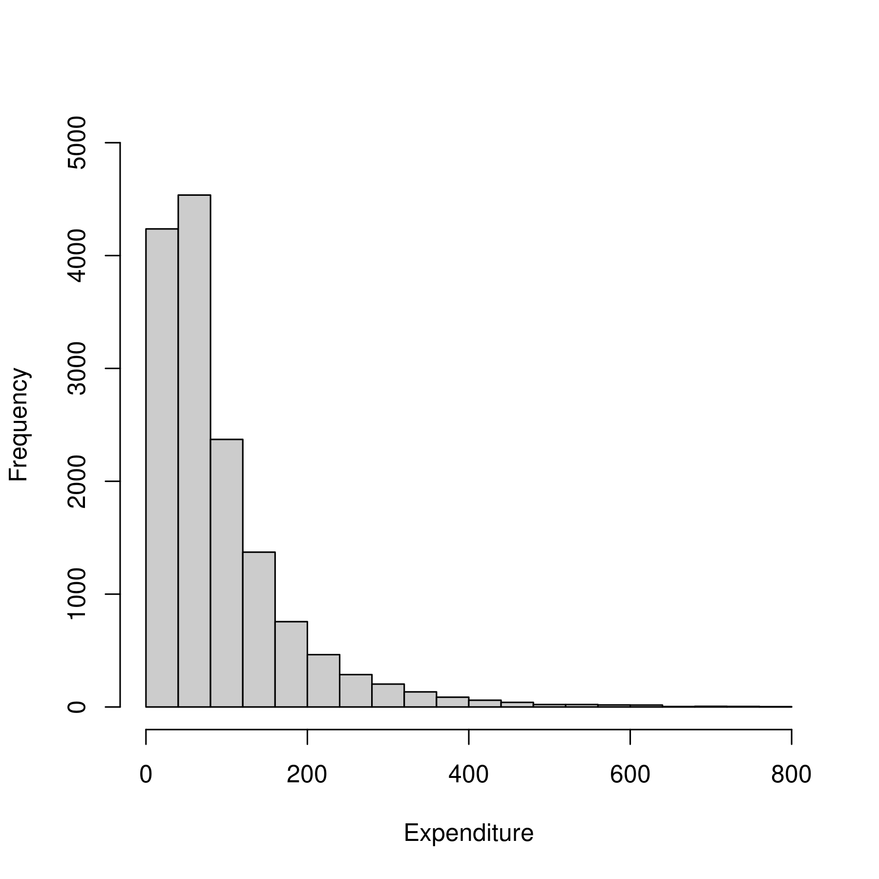
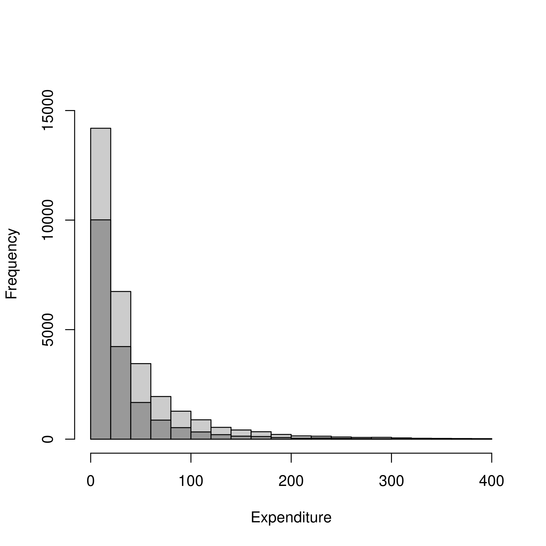
Figure 4: Sample Distributions of Expenditure $\tilde{y}$ by Regime. On the left, we illustrate the sample distribution conditional on $x_{1}>0$ and $x_{2}>0$; on the right, the light histogram illustrates the sample distribution conditional on $x_{1}=0$ and $x_{2}>0$, and the dark histogram illustrates the sample distribution conditional on $x_{1}>0$ and $x_{2}=0$.

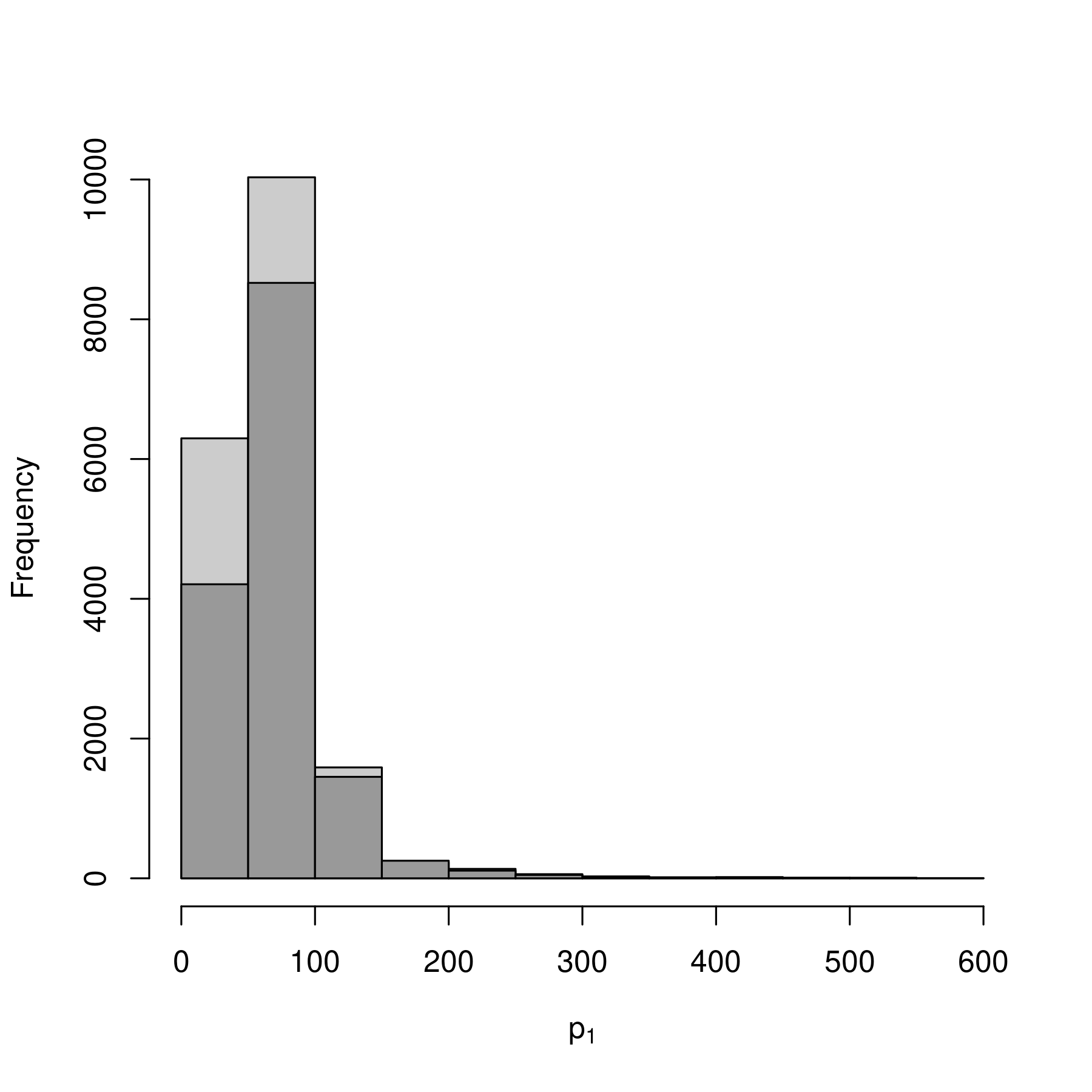
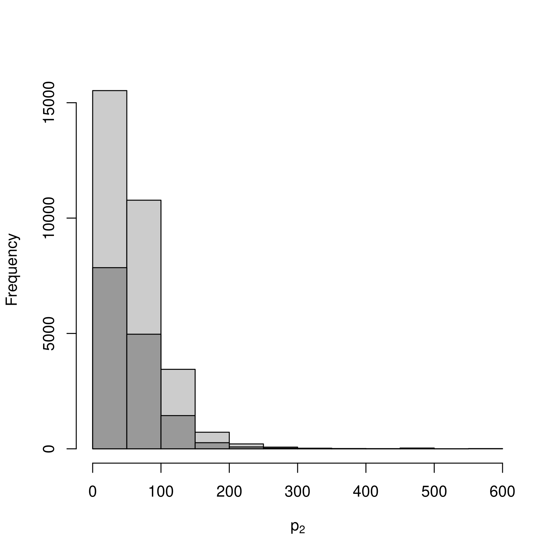
Figure 5: Sample Distributions of Prices $\tilde{p}_{j}$ by Regime. On the left, the light histogram illustrates the sample distribution of $\tilde{p}_{1}$ conditional on $x_{1}>0$ and $x_{2}=0$; on the right, the light histogram illustrates the sample distribution of $\tilde{p}_{2}$ conditional on $x_{1}=0$ and $x_{2}>0$; in each plot, the dark histogram illustrates the sample distribution conditional on $x_{1}>0$ and $x_{2}>0$.

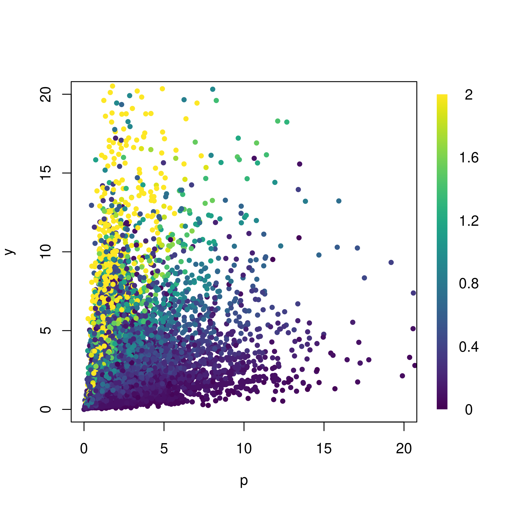
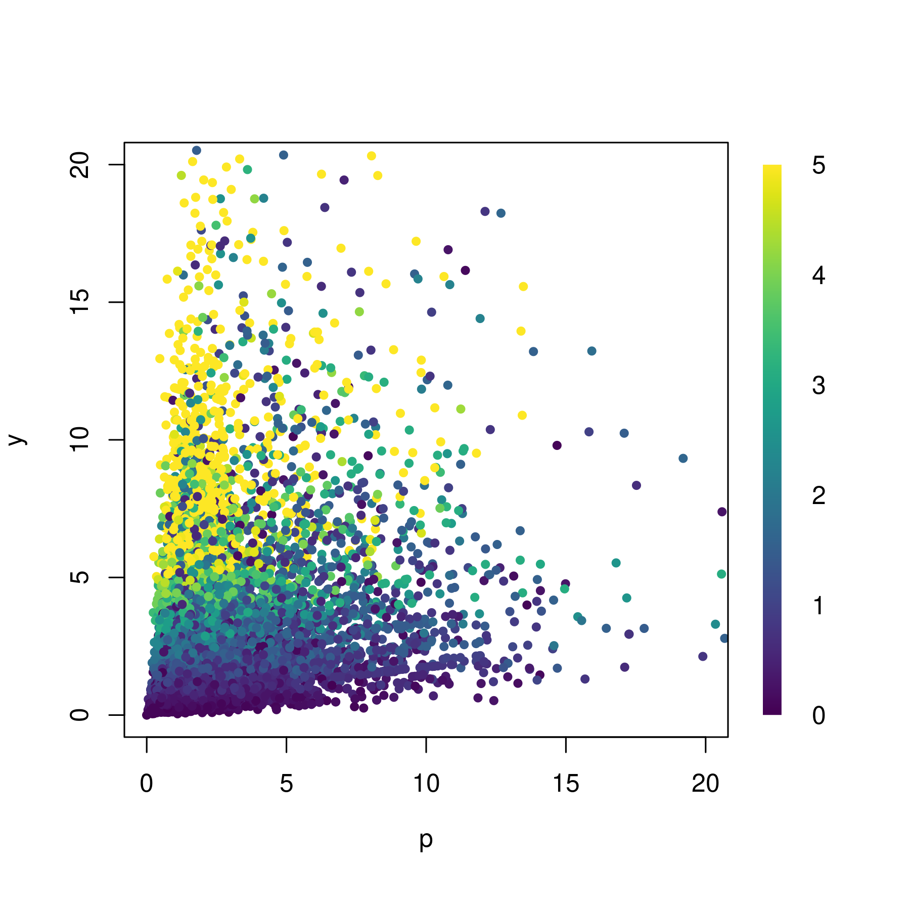
Figure 6: Sample Distributions of Designs $z_{it}$ and Consumption. These figures are conditional on $x_{it}>0$. On the left, colour describes the quantity of good 1; on the right, colour describes the quantity of good 2.

Since we consider a rather short window of time, we follow the segmented population approach. We segment the population by state. Large states (e.g. California) are segmented again by county. Specifically, a county is given its own segment if it has more than 70 observations with positive consumption and it is in a state with more than 1,000 observations with positive consumption. We are left with a total of 65 seg- ments, each corresponding to a state or county. The smallest segment is Wyoming, containing 15 observations with positive consumption; the largest state is Florida (after removing Broward, Hillsborough, Palm Beach, Pinellas, and Miami-Dade counties), containing 880 observations with positive expenditure; the mean number of observations with positive consumption per segment is approximately 226.

Figure 7 displays the sample distributions of (normalized) designs $z_{it}=(y_{it},p_{it})$ and the first component of consumption $x_{it}$ given $x_{it}>0$ in two of the larger segments: California (after removing Almeda, Los Angeles, Orange, Riverside, Sacramento, San Bernardino, and San Diego counties), and Florida (after removing Broward, Hillsborough, Palm Beach, Pinellas, and Miami-Dade counties).

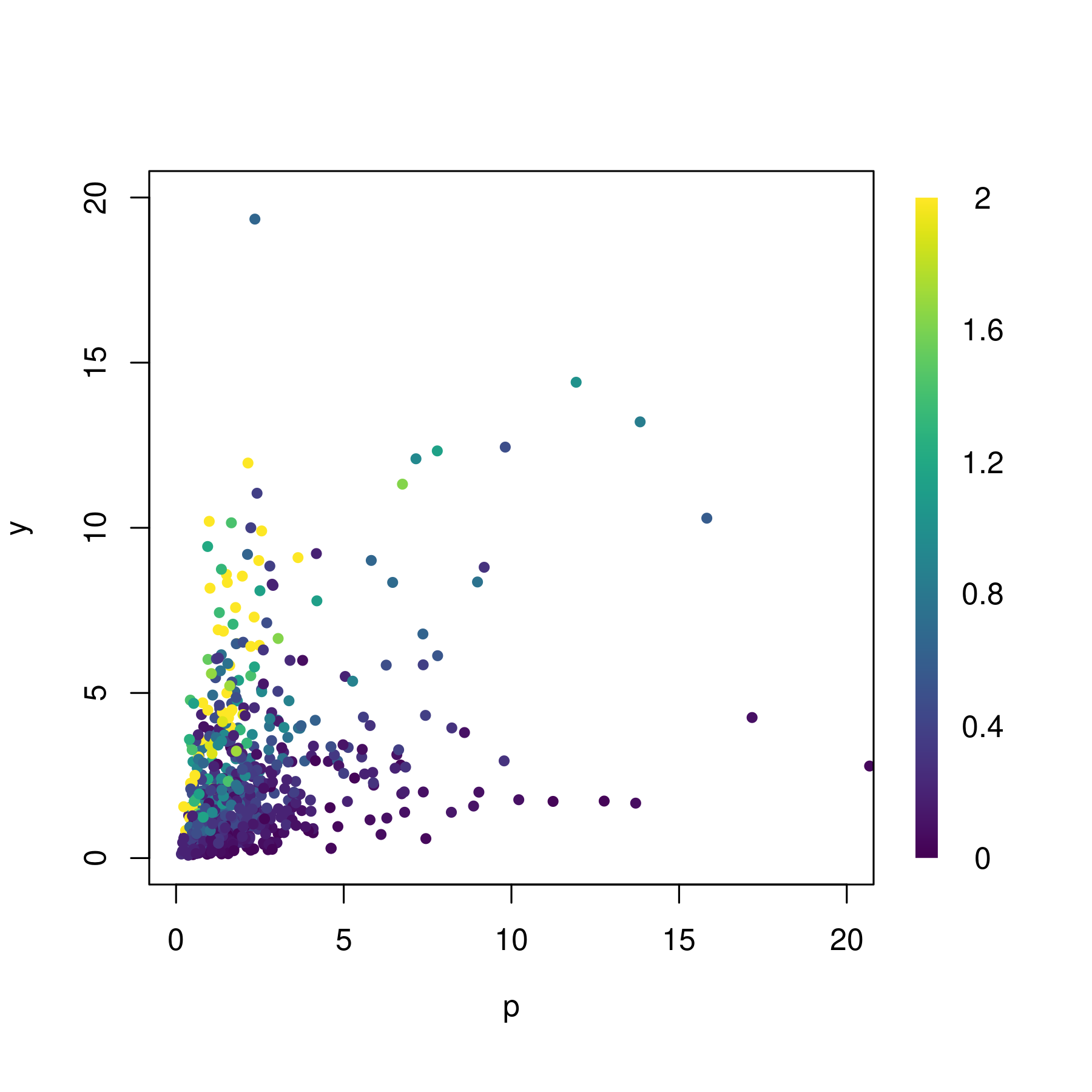
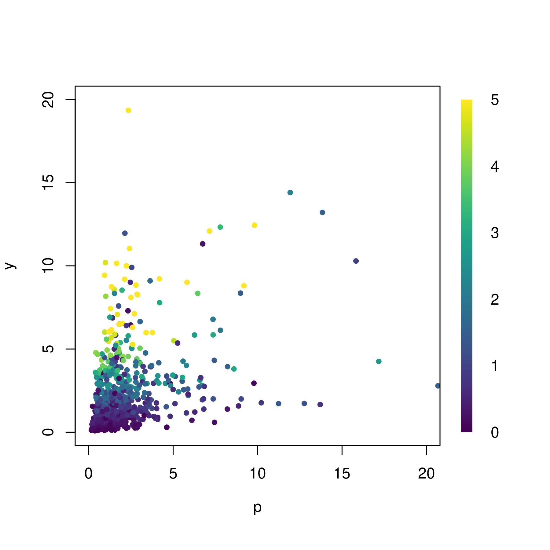
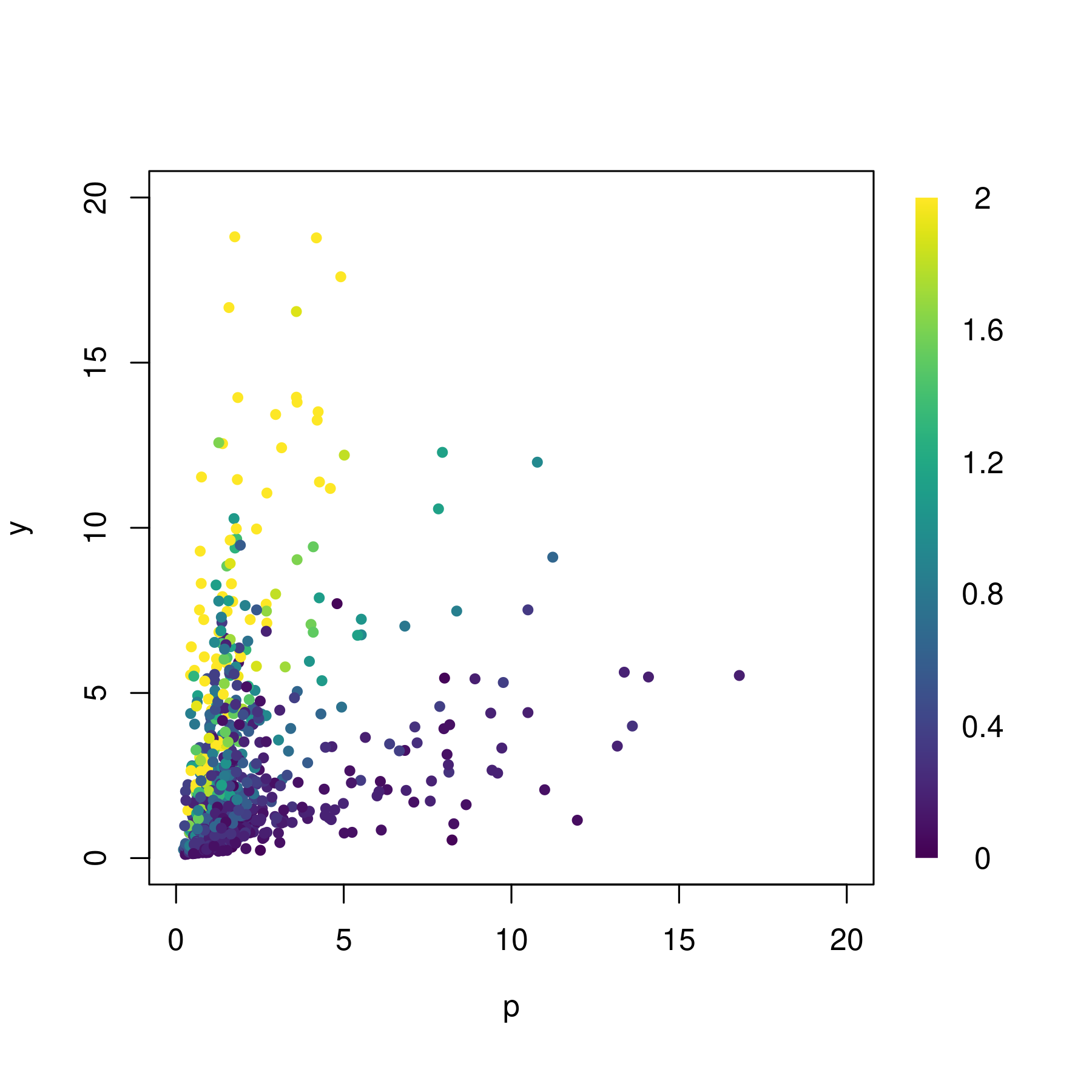
Figure 7: Sample Distributions by State. These figures are conditional on $x_{it}>0$. California is shown on the top, and Florida is shown on the bottom. On the left, colour describes the quantity of good 1; on the right, colour describes the quantity of good 2.

Figure 8 displays the Nadaraya-Watson (kernel) estimates of the demand function for beer conditional on $x_{it}>0$ in California and Florida over a subset of the domain of designs. Demand for beer in California is lower and less responsive to price changes than in Florida. Figure 9 displays Engel curves for good 1 in California and Florida given $p\equiv\tilde{p}_{1}/\tilde{p}_{2}=4$. These Engel curves cross.

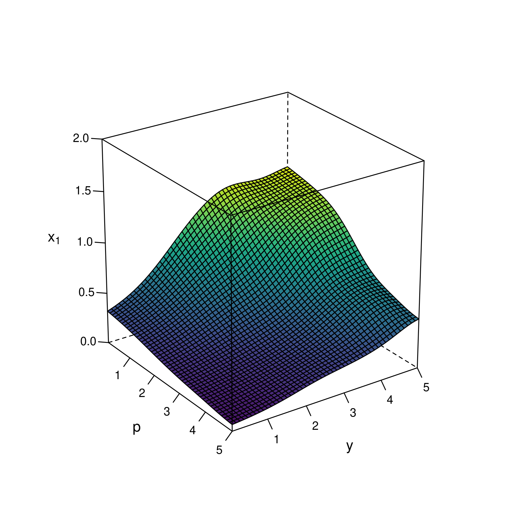
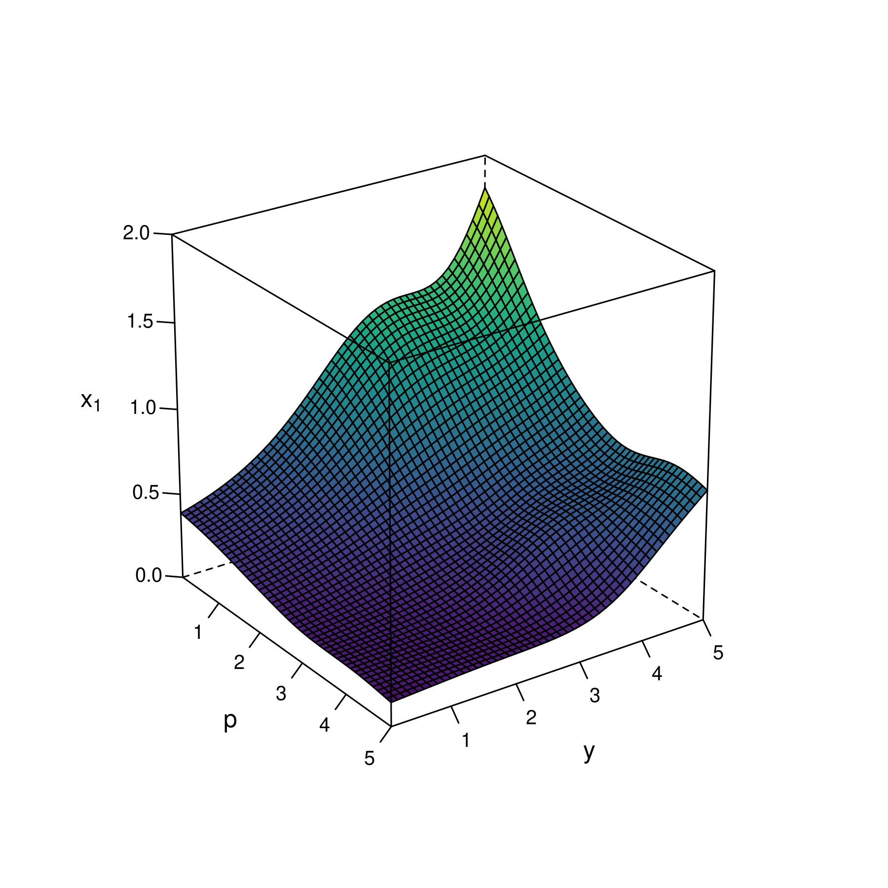
Figure 8: Demand. Nadaraya-Watson estimates of the demand function for good 1 conditional on $x_{it}>0$ in California (left) and Florida (right).

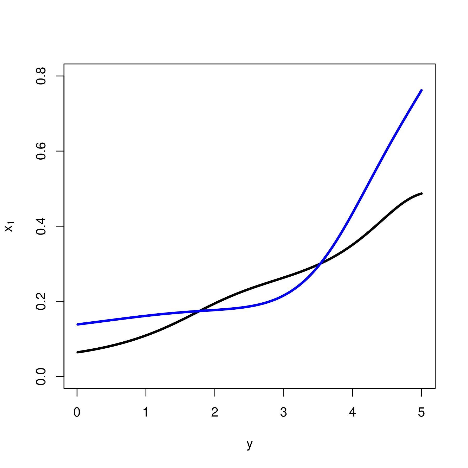
Figure 9: Engel Curves. Engel curves for good 1 in California (black) and Florida (blue). These curves violate monotonicity because they cross.

6.4 Estimation Results

As an illustration, we consider the SARA model in the hyperparametric framework. We assume that the taste parameters, $A_{1}$ and $A_{2}$, are independent. Under this assum- ption, the taste uncertainty is characterized by the marginal distributions, $\pi_{1}$ and $\pi_{2}$. The marginal distribution $\pi_{j}$ of $A_{j}$ is independently drawn from a Dirichlet process $F_{j}$, $j=1,2$. The mean of $F_{j}$ is a log-normal distribution with parameters $\mu_{j}$ and $\sigma_{j}$, and the scale parameter of $F_{j}$ is $c_{j}$. The utility function corresponding to this log-normal mean distribution, say $\bar{\pi}_{j}$, has a quasi closed-form expression. Indeed, under this distribution, we obtain:

$$\log(A_{j})=\mu_{j}+\sigma_{j}\varepsilon_{j},\;\;\forall j=1,2,$$

where $\varepsilon_{j}$ is distributed with respect to a standard normal distribution. Then:

$$\begin{gathered}\mathbb{E}_{\bar{\pi}_{j}}[\exp(-A_{j}x_{j})]=\mathbb{E}_{\bar{\pi}_{j}}[\exp(-\exp(\mu_{j}+\sigma_{j}\varepsilon_{j})x_{j})],\\ =\frac{1}{\sqrt{1+w(x_{j}\exp(\mu_{j})\sigma_{j}^{2})}}\exp\left\{-\frac{1}{2\sigma_{j}^{2}}w(x_{j}\exp(\mu_{j})\sigma_{j}^{2})^{2}-\frac{1}{\sigma^{2}}w(x_{j}\exp(\mu_{j})\sigma_{j}^{2})\right\},\end{gathered}$$

where $w(x)$ is the Lambert function, defined by the implicit equation:

$$w(x)\exp(w(x))=x,$$

[see equation (1.3) in Asmussen et al., 2016]. By drawing from the Dirichlet process, we will draw a stochastic utility function around the closed-form expression above. The hyperparameter $\theta$ has six components such that:

$$\theta=(\mu_{1},\sigma_{1},c_{1},\mu_{2},\sigma_{2},c_{2}).$$

6.4.1 The Hyperparameter

As described in Section 6.2.2, the first step involves estimating the hyperparameter $\theta$ using the Method of Simulated Moments (MSM). The hyperparameter $\theta$ is calibrated by using the following (sample and simulated) moments computed for all of the 63,936 observations with positive consumption:

1. marginal moments of $(X_{it})$;

2. cross-moments of $(\log X_{it},\log P_{it})$ and $(\log X_{it},\log Y_{it})$;

3. cross-moments of $(X_{it},P_{it})$, $(X_{it},Y_{it})$, $(X_{it},\log P_{it})$, and $(X_{it},\log Y_{it})$.

The moments in (ii) are the moments used in the Almost Ideal Demand System (see Deaton and Muellbauer, 1980); the moments in (iii) are introduced in order to capture risk effects by comparison with the moments in (ii). The optimum is found using a random search algorithm over a sufficiently big support.

To apply MSM, it is necessary to compute simulated consumption $x_{it}^{s}(\theta)$ for every observation, at each step of the optimization algorithm. This procedure is computati- onally costly. Note that, the number of simulated observations with positive consumption is stochastic, and not necessarily equal to the number of observations with positive consumption in the sample. This aspect has no impact on the consistency of the MSM estimator.

The estimated hyperparameter is:

$$\hat{\theta}=(0.7987,3.5516,45.0951,0.1201,3.6597,3.5544).$$ (6.4)

Therefore, the median level of risk aversion for the mean of the Dirichlet process for $A_{1}$ is $\exp(0.5495)\simeq 2.2226$, and the median level of risk aversion for the mean of the Dirichlet process for $A_{2}$ is $\exp(0.8738)\simeq 1.1276$. The fact that $\mu_{1}$ is smaller than $\mu_{2}$ is expected: Since quantities are measured in terms of volume of alcohol, this result is consistent with the faster overall intake of alcohol when consuming drinks with a higher ABV. Moreover, the distribution $\pi_{1}$ of $A_{1}$ is much more concentrated around its mean than the distribution $\pi_{2}$ of $A_{2}$, as the scaling parameter $c_{1}=45.0951$ for $\pi_{1}$ is much larger than the scaling parameter $c_{2}=3.5544$ for $\pi_{2}$.

We do not report any standard errors because they are automatically small from the large number of observations. Indeed, the standard significance test procedures (such as comparing a t-statistic to the critical value of a standard normal at the 5% significance level) are not relevant in this big data framework. The highest degree of uncertainty concerns the filtered functional parameters $(\hat{\pi}_{m})$ since $\pi_{m}$ is a high-dim- ensional parameter and the number of observations in each segment is much smaller.

The means of these Dirichlet processes are displayed in the left panel in Figure 10. The right panel displays the indifference curves associated with utility levels $-0.1000$, $-0.0800$, and $-0.0680$ for a draw from the Dirichlet process given $\hat{\theta}$.

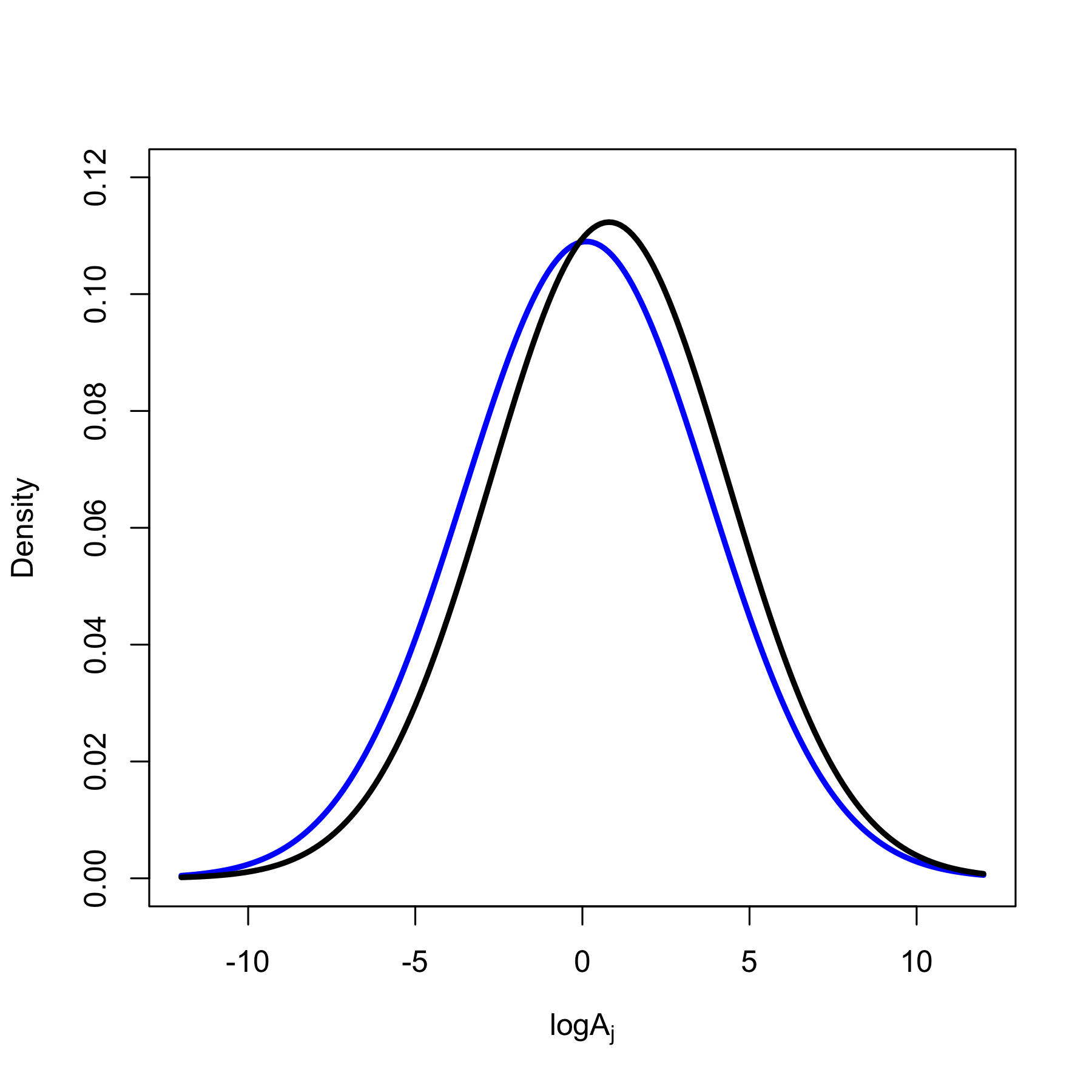
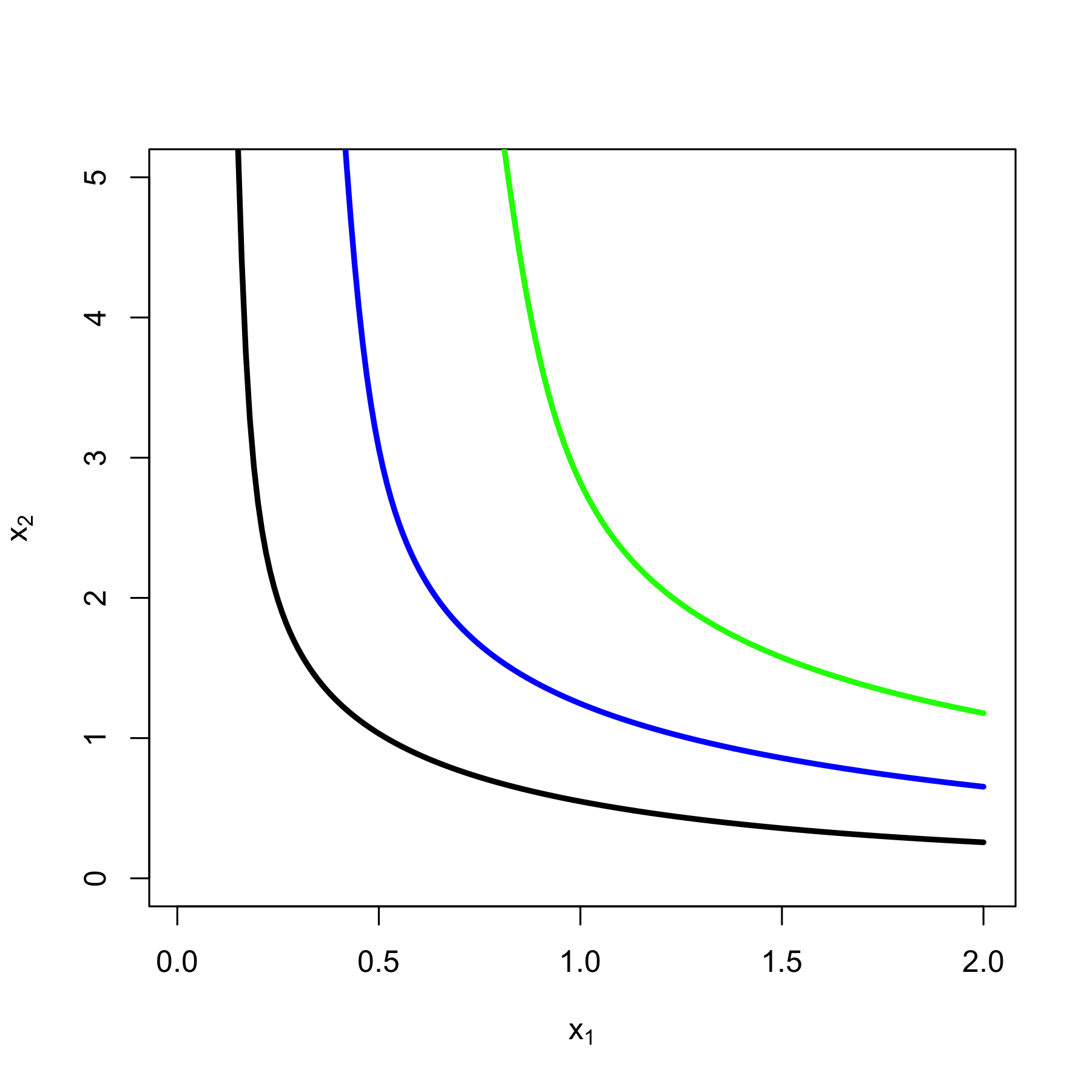
Figure 10: On the left, black shows the density of the mean of the Dirichlet process for $A_{1}$, and blue shows the density of the mean of the Dirichlet process for $A_{2}$. The $x$-axis is in log-scale. For scale: $\exp(-5)\simeq 0.0067$ and $\exp(5)\simeq 148.4131$. The figure on the right displays indifference curves associated with these distributions.

Figure 11 displays the Q-Q plots for two draws $(\pi_{1}^{s},\pi_{2}^{s})$, $s=1,2$, from the Dirichlet process given $\hat{\theta}$. In particular, we plot the quantiles of the realization of the distribution $\pi_{j}$ of $\log(A_{j})$ against the quantiles of the normal distribution given the estimated hyperparameters $(\hat{\mu}_{j},\hat{\sigma}_{j})$, for $j=1,2$. If these quantiles coincide exactly, they will lie on the 45-degree line. As expected, these Q-Q plots lie approximately around the 45-degree line. The draws $(\pi_{1}^{s})$, $s=1,2$, for $\pi_{1}$ are closer the 45-degree line and “more continuous” than the draws $(\pi_{2}^{s})$, $s=1,2$, for $\pi_{2}$ since $c_{1}>c_{2}$.

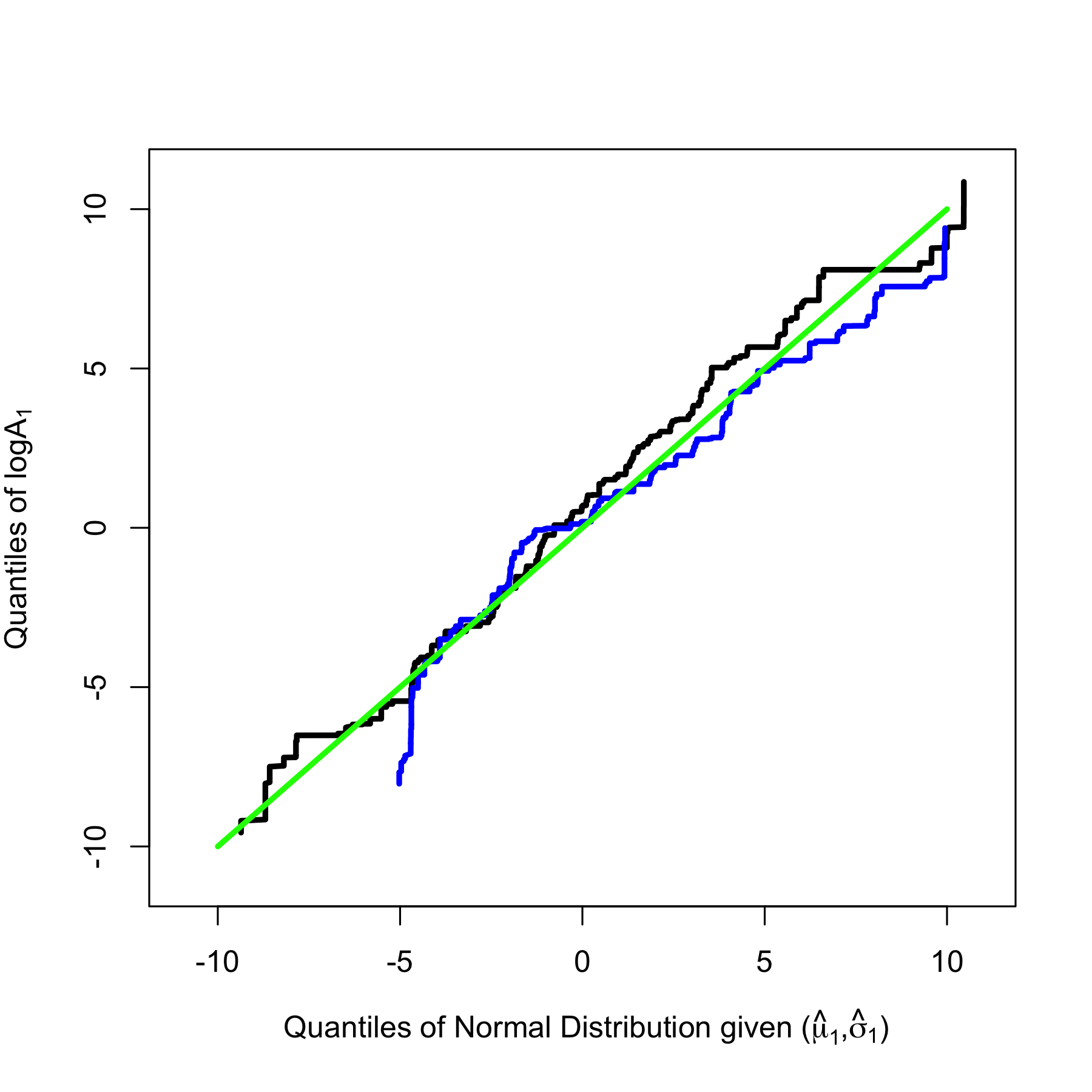
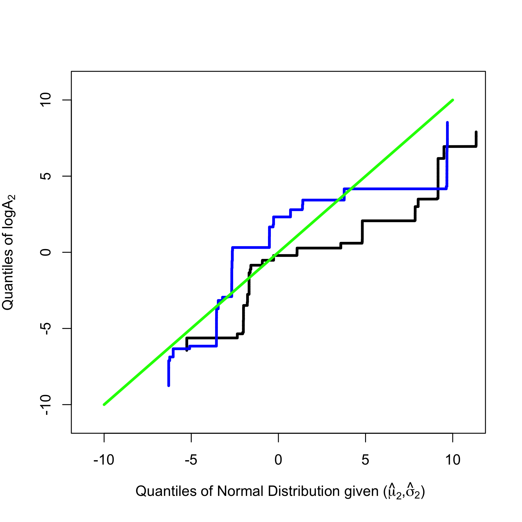
Figure 11: The Q-Q plots for two draws from the Dirichlet process given $\hat{\theta}$: On the left, the quantiles of $\log(A_{1})$ are plotted against the quantiles of the normal distribution given $(\hat{\mu}_{1},\hat{\sigma}_{1})$; on the right, the quantiles of $\log(A_{2})$ are plotted against the quantiles of the normal distribution given $(\hat{\mu}_{2},\hat{\sigma}_{2})$. In each figure, the green line is the 45-degree line.

Figure 11 illustrates how one might use the (estimated) hyperparameter for interpretation. Specifically, it is used to deduce the mean of the Dirichlet process, which is used as a benchmark for comparison with a drawn or filtered functional parameter $\pi_{m}$.

6.5 Taste Distributions

This section uses the filtering approach described in Section 6.2.4 to recover $\pi_{m}$. In the SARA model, the MRS restriction in (6.2) is:

$$\mathbb{E}_{\pi}[A_{1}\exp(-A^{\prime}x_{it})]=p_{it}\,\mathbb{E}_{\pi}[A_{2}\exp(-A^{\prime}x_{it})].$$

When $A_{1}$ and $A_{2}$ are independent, this expression becomes:

$$\begin{gathered}\mathbb{E}_{\pi_{1}}[A_{1}\exp(-A_{1}x_{i1t})]\mathbb{E}_{\pi_{2}}[\exp(-A_{2}x_{i2t})]\\ =p_{it}\,\mathbb{E}_{\pi_{1}}[\exp(-A_{1}x_{i1t})]\mathbb{E}_{\pi_{2}}[A_{2}\exp(-A_{2}x_{i2t})].\end{gathered}$$ (6.5)

To filter $\pi_{m}$, these restrictions have to be imposed for every observation with positive consumption $x_{it}$ associated with segment $\Lambda_{m}$. In California, there are 688 MRS rest- rictions, and, in Florida, there are 880. Appendix C shows how to numerically solve the resulting optimization problem given the bilinearity of the MRS restrictions under independence.

The marginal taste distributions were filtered using a grid with 500 points between $\exp(-10)$ and $\exp(10)$, equally spaced on the log-scale. All draws from the estimated prior were simulated by the stick-breaking method given $J=1000$ breaks (see Appen- dix A). Exactly $S=100$ draws from the posterior were used to filter each distribution.

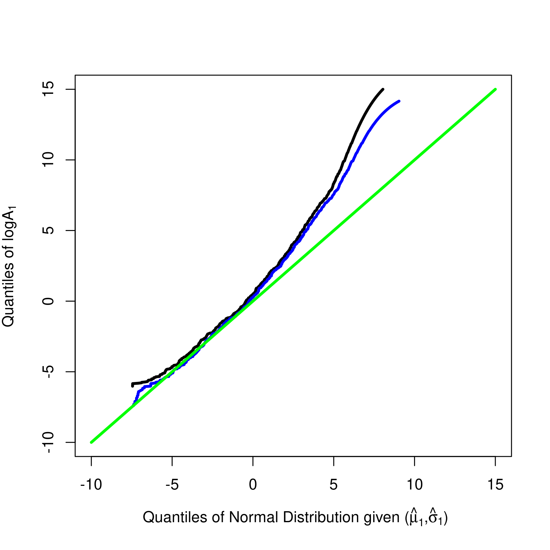
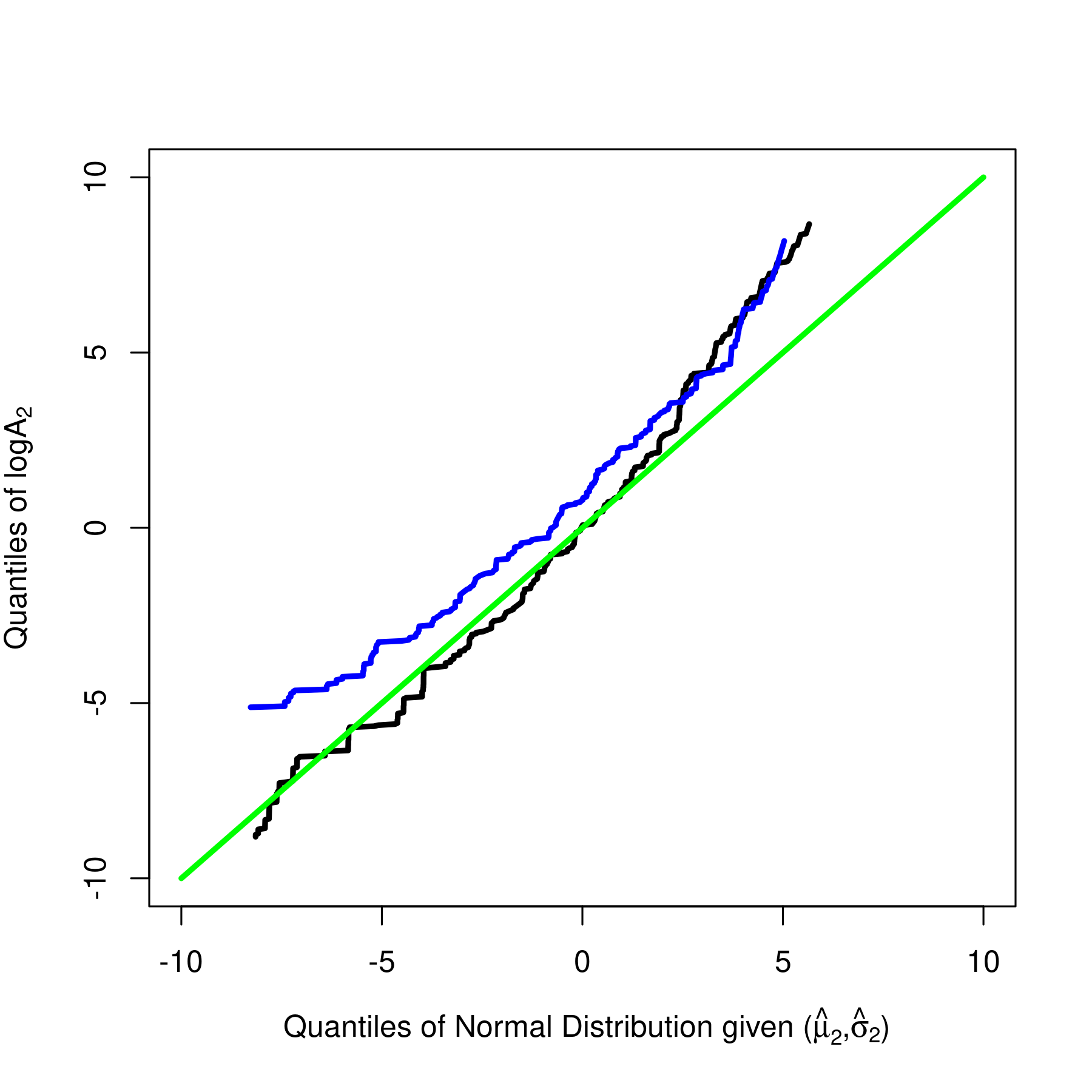
Figure 12: The Q-Q plots for the filtered taste distributions for California (black) and Florida (blue): On the left, the quantiles of $\log(A_{1})$ are plotted against the quantiles of the normal distribution given $(\hat{\mu}_{1},\hat{\sigma}_{1})$; on the right, the quantiles of $\log(A_{2})$ are plotted against the quantiles of the normal distribution given $(\hat{\mu}_{2},\hat{\sigma}_{2})$. In each figure, the green line is the 45-degree line.

Figure 12 displays the Q-Q plots for the filtered taste parameters $\hat{\pi}_{m}$ for California and Florida. As in Figure 11, the (estimated) hyperparameter is used to construct a benchmark for comparison. As expected, the filtered taste parameters are rather diff- erent from this benchmark. Here, the role of the estimated prior distribution diminishes with the number of observations. In both states, the slope on the left is steeper than the 45-degree line, suggesting that the posterior mean distribution for $A_{1}$ is more “dispersed” than its estimated prior mean distribution. The convexity of these curves also suggests fatter tails.

For the structural interpretation of these plots, assume that (i) the preferences are SARA, (ii) the taste parameters are independent, (iii) the marginal distribution of $A_{1}$ is the same in both states, and (iv) the marginal distribution of $A_{2}$ “shifts” such that $\pi_{2}^{*}(A_{2})=\pi_{2}(cA_{2})$, where $\pi_{2}$ and $\pi_{2}^{*}$ denote the marginal distributions of $A_{2}$ in these states. Under these assumptions:

$$U(x_{1},x_{2};\pi^{*})=U(x_{1},cx_{2};\pi),$$ (6.6)

and solving the utility maximization problem in (2.13) yields:

$$X_{1}(z;\pi^{*})=X_{1}(cz;\pi)\;\;\text{and}\;\;X_{2}(z;\pi^{*})=\left(\frac{1}{c}\right)X_{2}(cz;\pi).$$ (6.7)

Similarly, if there is a “shift” in the marginal distribution of $A_{1}$ and the marginal dist- ribution of $A_{2}$ is the same in both states, we obtain:

$$X_{1}(z;\pi^{*})=\left(\frac{1}{c}\right)X_{1}\left(y,\frac{p}{c};\pi\right)\;\;\text{and}\;\;X_{2}(z;\pi^{*})=X_{2}\left(y,\frac{p}{c};\pi\right).$$ (6.8)

The relationships given in (6.7) and (6.8) suggest that there exists a complicated non-linear relationship between such demand functions. Therefore, we cannot immediately deduce from Figure 12 which state has a higher demand for beer. For a more formal analysis, the utility functions associated with each posterior mean taste distribution must be used to derive a posterior MRS, or a posterior demand function.

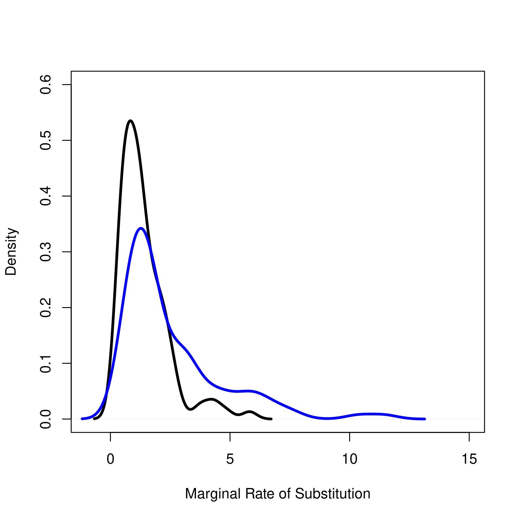
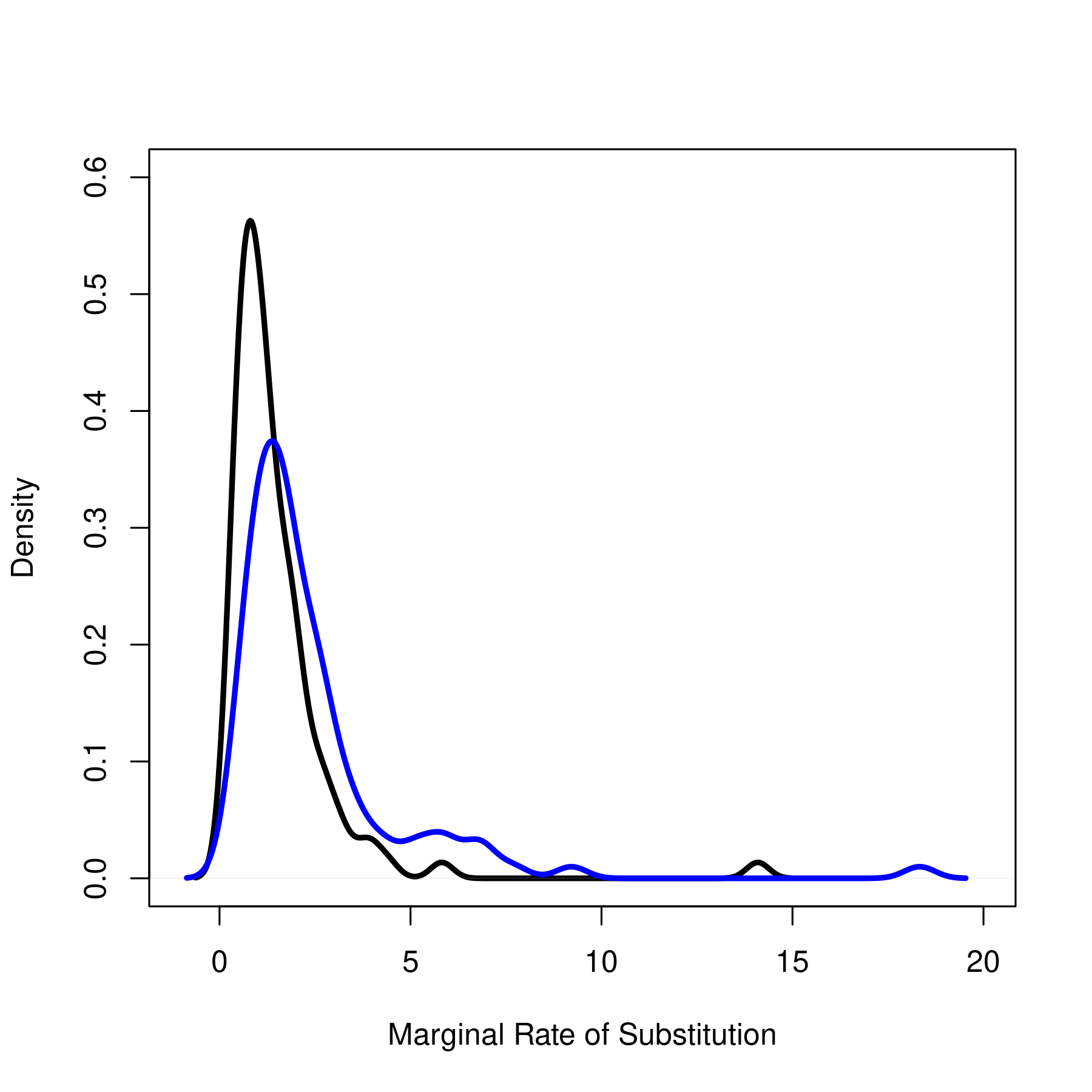
Figure 13: Posterior Marginal Rate of Substitution. The posterior distributions for $\text{MRS}(1,1;\pi)$ (black) and $\text{MRS}(1,2;\pi)$ (blue) for California (left) and Florida (blue).

This analysis has to be completed with a discussion of accuracy. In this non-param- etric framework, the posterior distributions of $\pi_{1}$ and $\pi_{2}$ are infinite-indimesional and cannot be represented. However, posterior distributions of any scalar transformation of $\pi_{1}$ and $\pi_{2}$ can be derived using simulation. In this respect, it is important to know which scalar objects are of interest. Typically, we are interested in the MRS evalu- ated at a specific bundle, say $x_{0}$, or counterfactual demand, corresponding to a particular design, say $z_{0}=(y_{0},p_{0})$. Figure 13 displays the posterior distributions of the MRS, evaluated at two bundles, $(1,1)$ and $(1,2)$, for California and Florida. In both states, these distributions are approximately log-normal (with is consistent with Dobronyi and Gouriéroux, 2020), and the posterior for $\text{MRS}(1,2;\pi)$ has a much longer tail than the posterior for $\text{MRS}(1,1;\pi)$, implying that, the quantity of good 2 that must be given to the consumer in order to compensate her for one unit of good 2 (and keep her just as happy) is larger, on average, when she has more of good 2. This tail is longer in California.

The filtered taste distributions in Figure 12 are obtained by applying the algorithm in Appendix C and forcing the density $\pi_{m}$ to be non-negative at each iteration. The existence of negative “probabilities” can be a result of numerical uncertainty, the choice of grid, or misspecification. Specifically, it can arise if the consumer in segment $\Lambda_{m}$ does not maximize her SARA/SSF utility function (or any utility function) subject to the linear budget constraint. By analyzing these negative probabilities, we can construct a measure of the deviation from rationality. To illustrate, let $\pi_{k}^{+}=\max\{0,\pi_{k}\}$ and $\pi_{k}^{-}=\max\{0,-\pi_{k}\}$, respectively, denote the positive and negative components of the elementary probability $\pi_{k}$ associated with the $k^{th}$ grid point. The following ratio:

$$\text{BR}=\frac{\sum_{k}\pi_{k}^{-}}{\sum_{k}(\pi_{k}^{-}+\pi_{k}^{+})},$$ (6.9)

is a measure of bounded rationality. This ratio ranges between 0 and 1. The closer this ratio is to 1, the less compatible the data are with the hundreds of MRS restrictions imposed by the chosen model. This ratio is related to a subset of the literature conce- rned with such measures. Existing measures include Afriat’s Efficiency Index (Afriat, 1967; Varian, 1990), and the Money Pump Index (Echenique et al., 2011). In general, these indices are used to measure a single consumer’s deviation from rationality by evaluating how “close” her choices are to satisfying the Generalized Axiom of Revealed Preference (GARP), a necessary and sufficient condition for a finite number of choices to be consistent with the maximization of any locally non-satiated utility function. In our framework, the BR ratio can be used to measure the violation of the homogeneous segment assumption. Table 3 displays the BR ratios for California and Florida. The BR ratio for $\pi_{1}$ is smaller than the ratio for $\pi_{2}$ in each state; these ratios are roughly the same across states.

Table 3: BR ratios for California and Florida.

State	$\pi_{1}$	$\pi_{2}$
California	0.15	0.20
Florida	0.17	0.21

7 Concluding Remarks

This paper is one among pioneering papers attempting to tackle the challenges of performing structural demand analysis with scanner data (see also Burda et al., 2008, 2012, Crawford and Polisson, 2016, Guha and Ng, 2019, Chernozhukov et al., 2020, and citecite.dobronyiDobronyi and Gouriéroux, 2020). The recent availability of scanner data permits new developments in the analysis of consumer behaviour. Here, we have shown that, by introducing homogeneous segments of consumers, we can consider a model of consumption with non-parametric preferences and infinite-dimensional heterogeneity, not only from a theoretical point-of-view, but also from a practical one. The distribution of individual heterogeneity in the population can be estimated, and the underlying non-parametric preferences can be filtered by using appropriate algorithms.

We developed an analysis for two goods for exposition. This feature of our analysis leaves the question: Can the methods developed in this paper be extended to a framework with, say, 100 goods? A completely unconstrained non-parametric analysis wou- ld encounter the curse of dimensionality. Specifically, we would need to estimate the distribution of the utility function (a non-parametric function with, in this scenario, 100 arguments). This task would be infeasible, even in our big data framework. But, the SARA model with independent taste parameters is a constrained non-parametric model. The structure of the SARA model reduces the non-parametric dimension of the problem, making it feasible. Indeed, when taste parameters are independent, we only need to estimate 100 one-dimensional distributions. A similar remark applies to the algorithm used to filter the taste distributions: The two steps based on the bilinear form of the MRS restrictions in a two good setting can be replaced with 100 successive steps based on the multilinear form of MRS restrictions in a 100 good setting, without increasing the numerical complexity.

Many of the results in this paper require taste parameters to be independent, but this requirement can be relaxed. For example, we can always consider a SARA model with the following form:

$$U(x;A)=-\exp(-(A_{c}+A_{1})x_{1}-(A_{c}+A_{2})x_{2}),$$ (7.1)

where $A_{c}$ is a common component, and $A_{j}$ is a good-specific taste parameter, for each $j=1,2$. In such a framework, independence between $A_{c}$, $A_{1}$, and $A_{2}$ does not imply independence between the parameters:

$$A_{1}^{*}=A_{c}+A_{1}\;\;\text{and}\;\;A_{2}^{*}=A_{c}+A_{2},$$ (7.2)

but it does reduce the dimensionality of the problem: Instead of introducing a joint distribution $\pi$ on a space of dimension 2, the model only depends on three distributions on a space of dimension 1. This specification avoids the curse of dimensionality. (See Appendix E for a discussion of identification in this case with taste dependence.)

In this paper, consumers are assumed to be rational, and divided into homogeneous segments. Since, in each segment, the demand function can be non-parametrically estimated over a subset of its domain, the analysis can be continued to develop a test of the homogeneity of each segment, or, more generally, a non-parametric method for constructing homogeneous segments.

The approach developed in this paper uses standard ideas from consumer theory to make inference. This approach is appropriate when both quantities and prices have continuous supports. This feature makes this approach valid for some levels of good, consumer, and date aggregation. Hence, this approach can be used for, say, evaluating the effect of alcohol tax on alcohol consumption, but unreasonable for analyzing how a particular consumer will choose between hundreds of different brands of whiskey. To our knowledge, the tools needed to solve such a problem have not been developed yet.

Appendix A The Dirichlet Process

In this appendix, we briefly review the definition and properties of the Dirichlet proc- ess, and then describe how to simulate from the Dirichlet process (see Ferguson, 1974, Rolin, 1992, Sethuraman, 1994, Lin, 2016, and Li et al., 2019).

A.1 Definition and Properties of the Dirichlet Process

For exposition, let us describe the Dirichlet distribution, then the Dirichlet process:

1. Dirichlet Distribution:

   Let $D_{J}(\alpha)$ denote the $J$-dimensional Dirichlet distribution with density:

   $$f_{\alpha}(q)=\frac{\Gamma\big{(}\sum_{j=1}^{J}\alpha_{j}\big{)}\prod_{j=1}^{J}q_{j}^{\alpha_{j}}}{\prod_{j=1}^{J}\Gamma(\alpha_{j})},$$ (A.1)

   for every $q\in[0,1]^{J}$ such that $\sum_{j=1}^{J}q_{j}=1$, where $\alpha\in\mathbb{R}_{++}^{J}$ denotes a $J$-dimensional vector of positive parameters. If a random vector $(Q_{1},\dots,Q_{J})$ has a Dirichlet distribution $D_{J}(\alpha)$, then:

   $$\mathbb{E}[Q_{j}]=\bar{\alpha}_{j}\quad\text{and}\quad V(Q_{j})=\frac{\bar{\alpha}_{j}(1-\bar{\alpha}_{j})}{1+\sum_{j=1}^{J}\alpha_{j}},$$ (A.2)

   where $\bar{\alpha}_{j}=\alpha_{j}/\sum_{j=1}^{J}\alpha_{j}$.

2. Dirichlet Process:

   In the SARA and SSF models, there are two taste parameters, $A_{1}$ and $A_{2}$. The probability distribution $\pi$ of $(A_{1},A_{2})$ is defined on $\mathbb{R}_{+}^{2}$. Therefore, in this section, we describe the Dirichlet process in this special case. Let $\mathscr{B}_{0}$ denote the Borel sets associated with $\mathbb{R}_{+}^{2}$, $\mathscr{F}$ denote the set of probability measures defined on $(\mathbb{R}_{+}^{2},\mathscr{B}_{0})$, and $\mathscr{B}_{1}$ denote the $\sigma$-algebra consisting of the Borel sets associated with the topology of weak convergence on $\mathscr{F}$. Let $\mu$ denote a (deterministic) probability measure defined on $(\mathbb{R}_{+}^{2},\mathscr{B}_{0})$, and let $c$ denote a strictly positive scalar. A process $G$ with values in $\mathscr{F}$ is a Dirichlet process with functional parameter $\mu$ and scaling parameter $c$ if, for every finite and measurable partition $\{C_{1},\dots,C_{J}\}$ of $\mathbb{R}_{+}^{2}$, the random vector $\big{[}G(C_{1}),\dots,G(C_{J})\big{]}^{\prime}$ has a $J$-dimensional Dirichlet distribution given $\alpha=\big{[}c\mu(C_{1}),\dots,c\mu(C_{J})\big{]}^{\prime}$. There exists a Dirichlet process for every probability measure $\mu$ defined on $(\mathbb{R}_{+}^{2},\mathscr{B}_{0})$ and scaling parameter $c$. The distribution of the Dirichlet process is a probability measure defined on $(\mathscr{F},\mathscr{B}_{1})$, whose realizations are almost surely discrete probability measures defined on $(\mathbb{R}_{+}^{2},\mathscr{B}_{0})$, assigning probability one to the set of all discrete probability measures defined on $(\mathbb{R}_{+}^{2},\mathscr{B}_{0})$. The support of the distribution of the Dirichlet process is a set of distributions with support contained in the support of $c\mu$ (Ferguson, 1974). The functional parameter $\mu$ (sometimes called the base distribution) can be thought of as the mean of the Dirichlet process—indeed, for any measurable set $C$ in $\mathbb{R}_{+}^{2}$, the mean of the Dirichlet distribution in (A.2) yields $\mathbb{E}[G(C)]=\mu(C)$. Therefore, in our framework, $\mu$ represents the expected uncertainty on taste parameters. Intuitively, the scaling parameter $c$ describes the “strength” of discretization: When $c$ is large, the realizations of the Dirichlet process are concentrated around $\mu$; loosely, as $c$ tends to infinity, the realizations become “more continuous.”

A.2 Simulating a Dirichlet Process

A Dirichlet process is easy to simulate given $\mu$ and $c$. There are a number of ways to simulate a realization—this section outlines the stick-breaking method, appropriate for drawing under the independence of $A_{1}$ and $A_{2}$, based on the construction of the Dirichlet process in Sethuraman (1994).

Let $B(\alpha_{1},\alpha_{2})$ denote the beta distribution with continuous density:

$$f(q)=\frac{\Gamma(\alpha_{1}+\alpha_{2})q_{1}^{\alpha_{1}}q_{2}^{\alpha_{2}}}{\Gamma(\alpha_{1})\Gamma(\alpha_{2})},$$ (A.3)

on the simplex $\{(q_{1},q_{2})\geq 0:q_{1}+q_{2}=1\}$, in which $\Gamma$ denotes the gamma function, and $\alpha_{1},\alpha_{2}>0$ are positive scalar parameters. Under the independence of $A_{1}$ and $A_{2}$, it is sufficient to be able to make a draw from a Dirichlet process whose realizations are distributions on $[0,\infty)$. Let $\mu^{*}$ and $c^{*}$ denote the mean and scaling parameter of this Dirichlet process. We can simulate from this process by using the following steps:

1. For large $L\geq 1$, independently simulate $W_{1},\dots,W_{L}\sim B(1,c^{*})$.

2. Compute $W_{1}^{*}=W_{1}$, and:

   $$W_{\ell}^{*}=W_{\ell}\prod_{j=1}^{\ell-1}(1-W_{j}),\;\;\forall\ell=2,\dots,L.$$ (A.4)

3. Independently simulate $V_{1},\dots,V_{J}\sim\mu^{*}$.

4. Define:

   $$G(C)=\sum_{\ell=1}^{L}W_{\ell}^{*}\delta_{V_{\ell}}(C),\;\;\forall C\subseteq\mathbb{R}_{+}^{2},$$ (A.5)

   where $\delta_{v}$ denotes a point mass at $v\in\mathbb{R}_{+}^{2}$.

Theoretically, if we could simulate an infinite number of draws, then this procedure would produce a realization of the Dirichlet process associated with functional parameter $\mu^{*}$ and scaling parameter $c^{*}$. Since $L$ is finite, the resulting probability measure $G$ is a truncated approximation of a realization of such a process. Figure 14 displays a simulated realization from the Dirichlet process given log-normal $\mu^{*}$ with mean 0 and standard deviation 1 (where these parameters are interpreted on the log-scale) and scaling parameter $c=100$. This realization was simulated using the stick-breaking method given $L=100$.

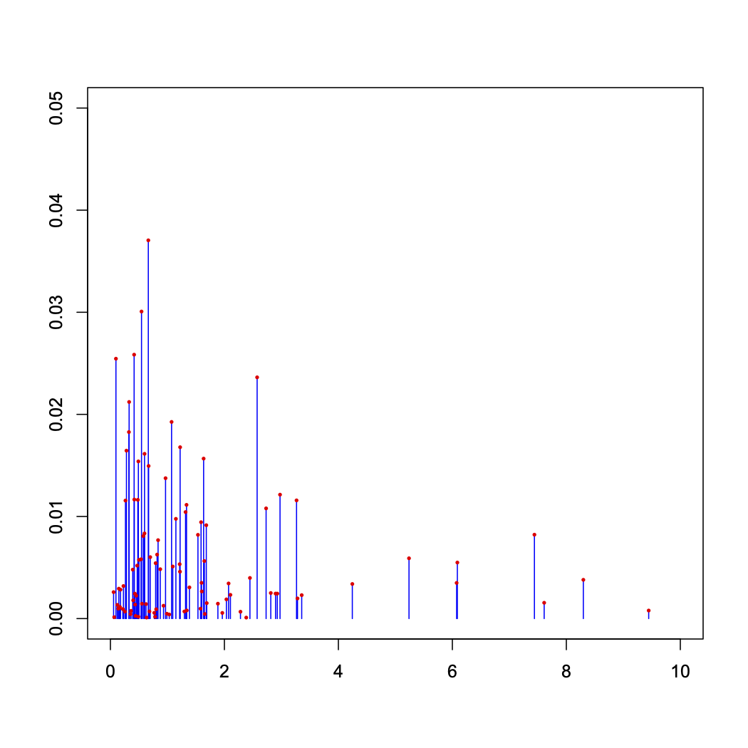
Figure 14: A simulated realization from the Dirichlet process given log-normal $\mu^{*}$ with mean 0 and standard deviation 1 (where these parameters are interpreted on the log-scale) and scaling parameter $c=100$. This realization was simulated using the stick-breaking method given $L=100$.

Appendix B Integrability

In each model, the Hessian of the utility function $U(x;\pi)$ is negative definite, implying that the demand function $X(z;\pi)$ is invertible in the second regime (see Proposition 2 in Dobronyi and Gouriéroux, 2020). Invertibility can also be analyzed using the indi- fference curves of $U(x;\pi)$, or the Slutsky coefficient $\Delta_{x}(z)$. As shown below, this anal- ysis can, for instance, yield new properties of the moment generating function (MGF).

B.1 SARA Model

Suppose $A_{1}$ and $A_{2}$ are independent. Let $\Psi_{j}$ denote the Laplace transform of $A_{j}$, for $j=1,2$. With this notation, we can write:

$$\log U(x;\pi)=\log\Psi_{1}(x_{1})+\log\Psi_{2}(x_{2}).$$ (B.1)

The indifference curve $g_{\pi}(\cdot,u)$ associated with $U(x;\pi)$ is obtained by solving:

$$\log\Psi_{1}(x_{1})+\log\Psi_{2}(x_{2})=\log u,$$ (B.2)

for $x_{2}$. This procedure leads to:

$$g_{\pi}(x_{1},u)=\left(\log\Psi_{2}\right)^{-1}\left(\log u-\log\Psi_{1}(x_{1})\right).$$ (B.3)

In general, demand is invertible if the indifference curves are strictly convex such that:

$$\frac{\partial^{2}g_{\pi}(x_{1},u)}{\partial x_{1}^{2}}>0,$$ (B.4)

for every $x_{1}>0$, and every attainable $u<0$. When preferences are SARA, we obtain:

$$\begin{split}\frac{d^{2}}{dv^{2}}&\left[\left(\log\Psi_{2}\right)^{-1}\right]\left(\log u-\log\Psi_{1}(x_{1})\right)\left(\frac{d\log\Psi_{1}(x_{1})}{dx_{1}}\right)^{2}\\ -\frac{d}{dv}&\left[\left(\log\Psi_{2}\right)^{-1}\right]\left(\log u-\log\Psi_{1}(x_{1})\right)\frac{d^{2}\log\Psi_{1}(x_{1})}{dx_{1}^{2}}>0,\end{split}$$ (B.5)

for every $x_{1}>0$, and every attainable $u<0$. These inequalities, involving two MGFs, are always satisfied. Consequently, we have derived a new property of the MGF, as described in the introduction of this appendix.

B.2 SSF Model

If preferences are SSF, it is rather challenging to derive a closed-form expression for the indifference curve. We can, instead, write the integrability condition using the condition on the bordered Hessian in Lemma 1 in Dobronyi and Gouriéroux (2020), but, for both brevity and exposition, let us simply restrict our attention to the general specification of utility in the example in Section 3.3 and check that integrability holds for any Laplace transform. Because the strict convexity of the indifference curves is equivalent to the strict negativity of the Slutsky coefficient $\Delta_{x}(z)$, it is sufficient to check whether $\Delta_{x}(z)$ is strictly negative. We obtain:

$$\begin{split}\Delta_{x}(z)&=\frac{\partial X_{1}(z;\pi)}{\partial p}+X_{1}(z;\pi)\frac{\partial X_{1}(z;\pi)}{\partial y}=-\frac{1}{\lambda p^{3}}\frac{d}{dv}\left(\frac{d\log\Psi}{dv}\right)^{-1}\left(-\frac{1}{p}\right).\end{split}$$ (B.6)

It is sufficient to show that:

$$\frac{d}{dv}\left(\frac{d\log\Psi}{dv}\right)^{-1}\left(-\frac{1}{p}\right),$$ (B.7)

is strictly positive. To do this, consider the following derivatives:

$$\begin{gathered}\frac{d\log\Psi(v)}{dv}=-\frac{\mathbb{E}[A_{1}\exp(-A_{1}v)]}{\mathbb{E}[\exp(-A_{1}v)]},\\ \text{and}\;\;\frac{d^{2}\log\Psi(v)}{dv^{2}}=\frac{\mathbb{E}[A_{1}^{2}\exp(-A_{1}v)]}{\mathbb{E}[\exp(-A_{1}v)]}-\left(\frac{\mathbb{E}[A_{1}\exp(-A_{1}v)]}{\mathbb{E}[\exp(-A_{1}v)]}\right)^{2}=V_{\tilde{\pi}}(A_{1})>0,\end{gathered}$$ (B.8)

where the variance is with respect to the transformed density:

$$\frac{\exp(-A_{1}v)}{\mathbb{E}[\exp(-A_{1}v)]}\pi(v).$$ (B.9)

Therefore, $\frac{d\log\Psi}{dv}$ is increasing, and so is its inverse $\left(\frac{d\log\Psi}{dv}\right)^{-1}$. Thus, $\Delta_{x}(z)$ is negative.

Appendix C Numerical Optimization

The optimization problem for filtering can be written as:

$$\begin{gathered}\min_{\pi_{1},\pi_{2}}\;(\pi_{1}-\hat{\pi}_{1})^{\prime}(\pi_{1}-\hat{\pi}_{1})+(\pi_{2}-\hat{\pi}_{2})^{\prime}(\pi_{2}-\hat{\pi}_{2})\\ \text{s.t.}\;\;\text{MRS restrictions \eqref{mrsrestrictions2}, $e^{\prime}\pi_{1}=1$, and $e^{\prime}\pi_{2}=1$,}\end{gathered}$$ (C.1)

where $\pi_{1}$ and $\pi_{2}$ are written on a sufficiently large discrete grid for $A_{1}$ and $A_{2}$, and $e=(1,\dots,1)^{\prime}$. This optimization problem can be difficult due to the dimension of the problem. The objective function is minimized with respect to the total number $2J$ of grid points in $\pi_{1}$ and $\pi_{2}$, which is intentionally chosen to be very large (at least several hundred), and the number of constraints is $N_{m}$, where $N_{m}$ denotes the number of observations with positive consumption $x_{it}$ in segment $\Lambda_{m}$, which is typically around 1,000. Note, $2J$ has to be larger than $N_{m}$ for identification. Therefore, it is important to find a tractable algorithm for such a problem.

We can use the fact that the MRS restrictions are bilinear in $\pi_{1}$ and $\pi_{2}$. Indeed, these constraints can be written as:

$$A_{1}(\pi_{2})\pi_{1}=b_{1}(\pi_{2})\;\;\text{or}\;\;A_{2}(\pi_{1})\pi_{2}=b_{2}(\pi_{1}).$$ (C.2)

To illustrate, consider the SARA model, and let $a_{1j}$ and $a_{2j}$, $j=1,\dots,J$, denote the locations of the points in the grids for $A_{1}$ and $A_{2}$, respectively. Moreover, let $\pi_{1}=(\pi_{1j})$ and $\pi_{2}=(\pi_{2j})$ denote the elementary probabilities on $(a_{1j})$ and $(a_{2j})$, respectively. Under the independence of $A_{1}$ and $A_{2}$, the MRS restrictions have the form:

$$\begin{gathered}\sum_{j=1}^{J}[\pi_{1j}a_{1j}\exp(-a_{1j}x_{i1t})]\sum_{j=1}^{J}[\pi_{2j}\exp(-a_{2j}x_{i2t})]\\ -p_{it}\sum_{j=1}^{J}[\pi_{1j}\exp(-a_{1j}x_{i1t})]\sum_{j=1}^{J}[\pi_{2j}a_{2j}\exp(-a_{2j}x_{i2t})]=0,\end{gathered}$$

for every $i\in\Lambda_{m}$ and every $t$ with $x_{it}>0$. The closed-form expressions for $A_{1}(\pi_{2})$, $b_{1}(\pi_{2})$, $A_{2}(\pi_{1})$, and $b_{2}(\pi_{1})$ can be easily deduced. The unit mass restrictions can also be explicitly written as:

$$\sum_{j=1}^{J}\pi_{1j}=1\;\;\text{and}\;\;\sum_{j=1}^{J}\pi_{2j}=1.$$

The equivalent expressions in (C.2) can be used to solve the optimization problem in (C.1) by using a succession of optimization problems with smaller dimensions (see Gouriéroux et al., 1990, and Van Rosen, 2018). Precisely, let $\pi_{1}(k)$ and $\pi_{2}(k)$ denote the solutions for $\pi_{1}$ and $\pi_{2}$ at the $k^{th}$ step of the optimization algorithm. Given $\pi_{2}(k)$, $\pi_{1}(k+1)$ is defined as the solution to:

$$\min_{\pi_{1}}\;(\pi_{1}-\hat{\pi}_{1})^{\prime}(\pi_{1}-\hat{\pi}_{1})\;\;\text{s.t. $A_{1}[\pi_{2}(k)]\pi_{1}=b_{1}[\pi_{2}(k)]$ and $e^{\prime}\pi_{1}=1$},$$ (C.3)

and, similarly, $\pi_{2}(k+1)$ is defined as the solution to:

$$\min_{\pi_{2}}\;(\pi_{2}-\hat{\pi}_{2})^{\prime}(\pi_{2}-\hat{\pi}_{2})\;\;\text{s.t. $A_{2}[\pi_{1}(k+1)]\pi_{2}=b_{2}[\pi_{1}(k+1)]$ and $e^{\prime}\pi_{2}=1$}.$$ (C.4)

If this algorithm numerically converges, then the limit is the solution to the original optimization problem in (C.1). Moreover, $\pi_{1}(k)$ and $\pi_{2}(k)$ have closed-form solutions:

Proposition 8.

The solution to (C.3) is equal to:

$$\pi_{1}(k+1)=\hat{\pi}_{1}+A_{1}^{*}[\pi_{2}(k)]^{\prime}\big{\{}A_{1}^{*}[\pi_{2}(k)]A_{1}^{*}[\pi_{2}(k)]^{\prime}\big{\}}^{-1}\big{\{}b_{1}^{*}[\pi_{2}(k)]-A_{1}^{*}[\pi_{2}(k)]\hat{\pi}_{1}\big{\}},$$ (C.5)

where $A_{j}^{*}$ and $b_{j}^{*}$ encompass the MRS constraint and the unit mass contraint together.

Proof.

The optimization problem in (C.1) is of the following type:

$$\min_{w}\;(w-w_{0})^{\prime}(w-w_{0})\;\;\text{s.t.}\;\;Aw=b.$$

Let us introduce a Lagrange multiplier $\lambda$. The first-order conditions are, then:

$$2(w-w_{0})-A^{\prime}\lambda=0\;\;\text{and}\;\;Aw=b.$$ (C.6)

The first condition can be written as:

$$w=w_{0}+\frac{1}{2}A^{\prime}\lambda.$$ (C.7)

By plugging this expression for $w$ into the second condition, we obtain:

$$\frac{\lambda}{2}=(AA^{\prime})^{-1}(b-Aw_{0}).$$ (C.8)

Together, (C.7) and (C.8) imply:

$$w=w_{0}+A^{\prime}(AA^{\prime})^{-1}(b-Aw_{0}).$$

This expression is exactly the form of the solution in the statement of this proposition. ∎

Remark 1.

Instead of minimizing the $\ell_{2}$-distance between $\pi_{j}$ and $\hat{\pi}_{j}$, we could use an information criterion, as in Kitamura and Stutzer (1997). However, we would no longer obtain a closed-form solution for $\pi_{1}(k)$ and $\pi_{2}(k)$, and we would have to solve a non-linear system in $\lambda$ with dimension $N_{m}$.

Remark 2.

The inversion of $AA^{\prime}$ is numerically feasible, but can be made more robust numerically by including a regularization. In particular, it can be replaced with the inversion of $AA^{\prime}+\varepsilon I$, where $\varepsilon>0$ is a small regularization parameter. This regularization by shrinkage (see, for example, Ledoit and Wolf, 2004) is preferable to the machine learning practice which replaces $AA^{\prime}$ with the diagonal matrix made up of the diagonal elements of $AA^{\prime}$. In practice, it can also be easier to solve the system in (C.6), instead of using (C.5).

Remark 3.

The optimization problem in (C.1) has not explicitly accounted for the positivity of $\pi_{1}$ and $\pi_{2}$. We can incorporate positivity by adjusting after each step of the algorithm.

Appendix D The Nielsen Database

In this appendix, we provide more information about the Nielsen Homescan Consumer Panel (NHCP). First, we describe the individual records, then the representativeness of our restricted sample.

D.1 Individual Records

As mentioned in the text, all purchases are continuously recorded by each consumer. The left panel in Figure 15 displays the daily (total and alcohol-specific) expenditures of a given consumer in October of 2016. During this month, this consumer purchased 166 units of 97 distinct goods (prior to aggregation). The right panel in Figure 15 displays the daily number of units purchased by this consumer. These purchases were all made at three distinct retailers.

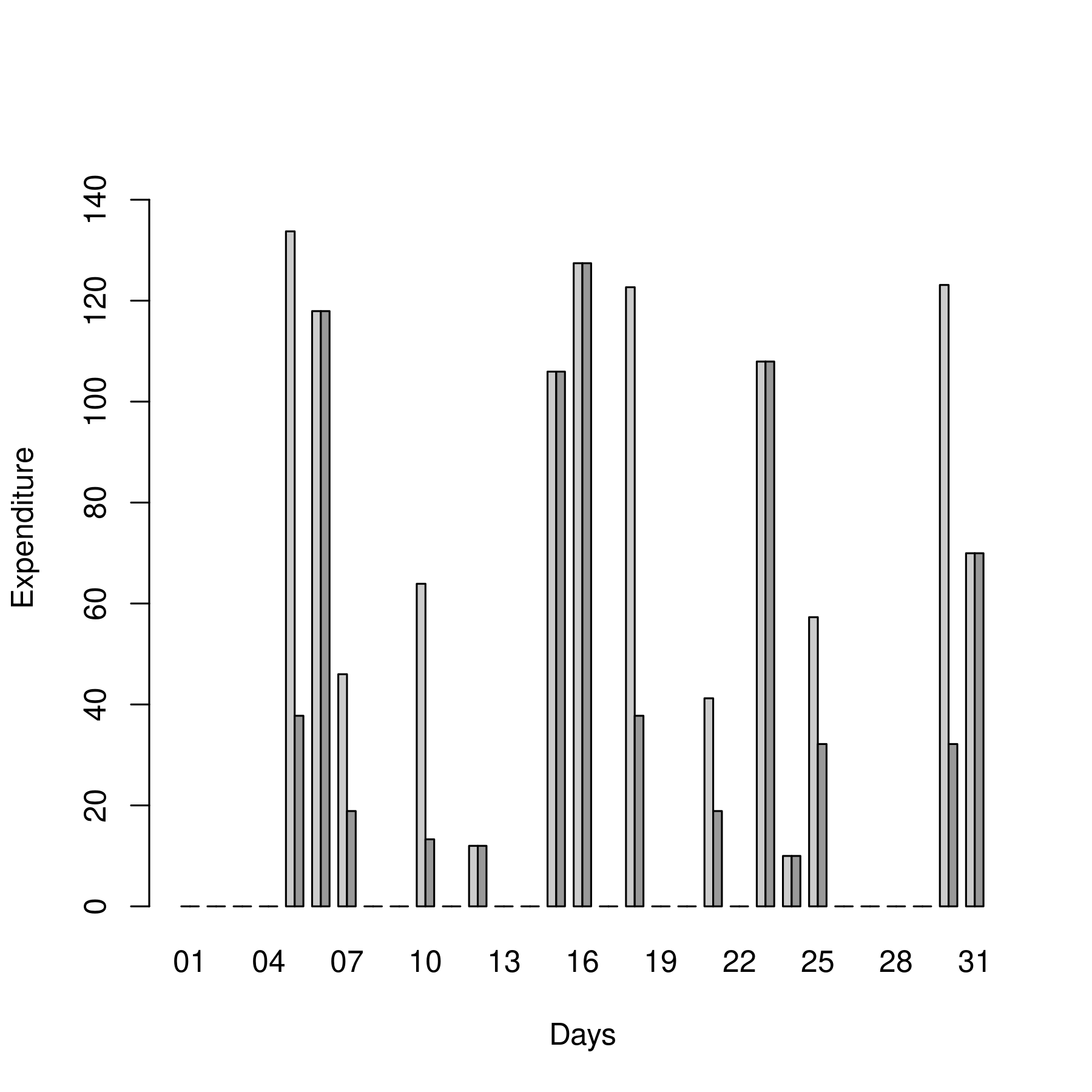
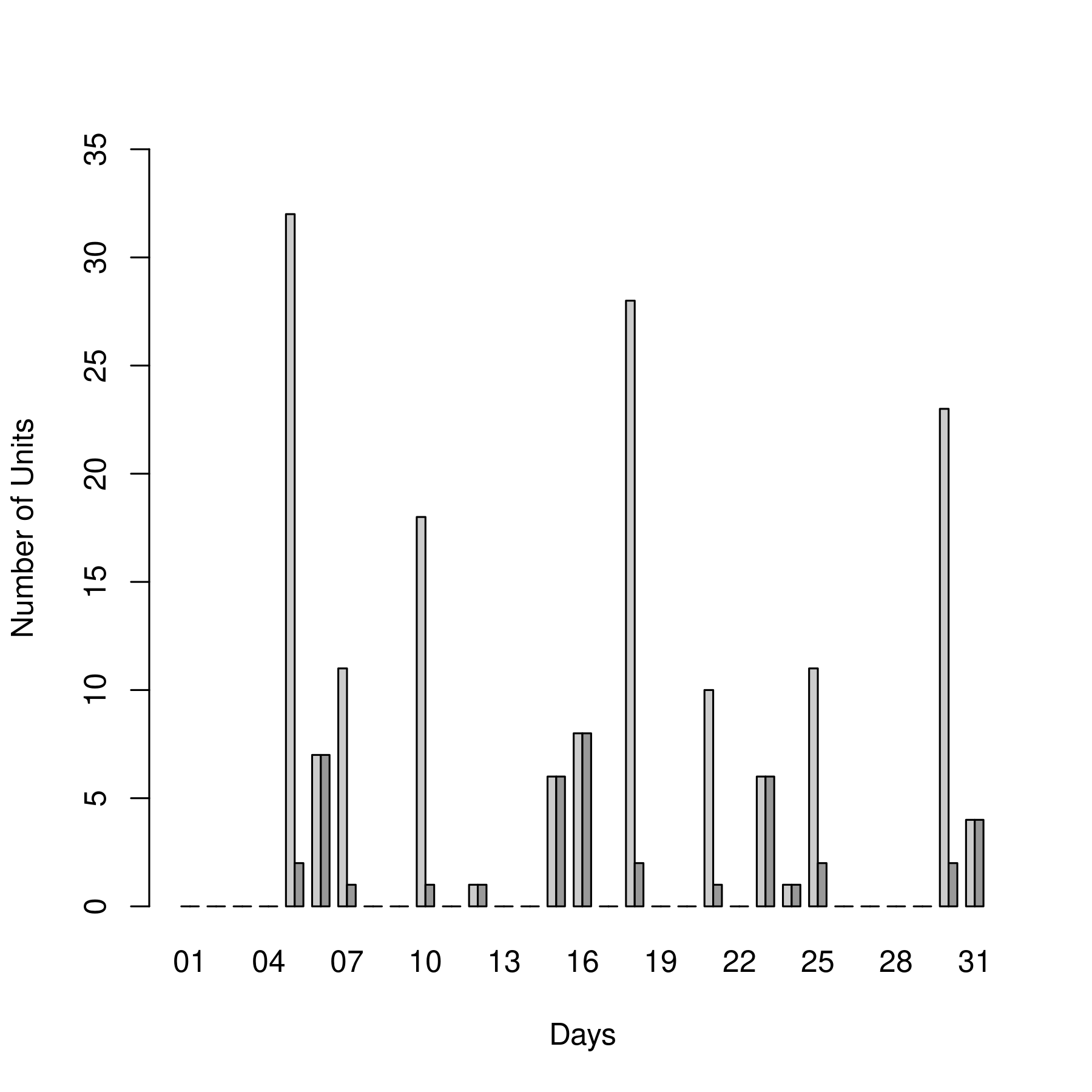
Figure 15: Daily Purchases. On the left, we illustrate daily expenditure for a single consumer in October of 2016. On the right, we illustrate the number of units purchased by this consumer. Light shaded bars represent all purchases and dark shaded bars represent alcohol-related purchases.

D.2 Representativeness of Sample

Let us now report the demographics of the households in our data and compare these demographics with the Current Population Survey (CPS). See Guha and Ng (2019) and Dobronyi and Gouriéroux (2020) for additional summary statistics.

Table 4 gives the distribution of household size in our sample and the CPS. These distributions are similar. Our sample has a slightly smaller proportion of households with a single member, and a slightly larger proportion of households with two members. This difference can be explained by single-member households simply buying less alcohol.

Table 4: Household size in our sample and in the 2017 Annual Social and Economic Supplement (ASEC) of the CPS. CPS numbers are in thousands.

	Sample		CPS
Size	Number	Proportion	Number	Proportion
1	5,862	0.2090	35,388	0.2812
2	12,768	0.4554	42,785	0.3400
3	4,121	0.1469	19,423	0.1543
4	3,395	0.1210	16,267	0.1292
5	1,288	0.0459	7,548	0.0599
6	422	0.0150	2,813	0.0223
7+	180	0.0064	1,596	0.0126
Total	28,036	1.0000	125,819	1.0000

Table 5 describes the distribution of household income in our sample and the CPS. Once again, these two distributions are quite similar, but our sample has a higher proportion of households earning between $70,000 and $99,999.

Table 5: Annual household income in our sample and in the 2017 Annual Social and Economic Supplement (ASEC) of the CPS. CPS numbers are in thousands.

	Sample		CPS
Income	Number	Proportion	Number	Proportion
Under $5,000	265	0.0094	4,138	0.0327
$5,000 to $9,999	274	0.0097	3,878	0.0307
$10,000 to $14,999	638	0.0227	6,122	0.0485
$15,000 to $19,999	694	0.0247	5,838	0.0462
$20,000 to $24,999	1,147	0.0409	6,245	0.0494
$25,000 to $29,999	1,282	0.0457	5,939	0.0470
$30,000 to $34,999	1,480	0.0527	5,919	0.0468
$35,000 to $39,999	1,432	0.0510	5,727	0.0453
$40,000 to $44,999	1,449	0.0516	5,487	0.0434
$45,000 to $49,999	1,637	0.0583	5,089	0.0403
$50,000 to $59,999	2,878	0.1026	9,417	0.0746
$60,000 to $69,999	2,380	0.0848	8,213	0.0650
$70,000 to $99,999	6,459	0.2303	19,249	0.1524
$100,000+	6,021	0.2147	34,963	0.2769
Total	28,036	1.0000	126,224	1.0000

Tables 6 gives the distribution of the age of the eldest head of the household in our sample and the age of the householder in the CPS. There is no direct comparison for these statistics, as the eldest head may differ from the householder. This aspect of the data can explain why our sample seems to be older than the general population.

Table 6: Age of eldest household head in our sample and the householder in the 2017 Annual Social and Economic Supplement (ASEC) of the CPS. CPS numbers are in thousands.

	Sample		CPS
Age	Number	Proportion	Number	Proportion
Under 20	4	0.0001	753	0.0059
20 to 24	54	0.0019	5,608	0.0445
25 to 29	476	0.0169	9,453	0.0751
30 to 34	1,201	0.0428	10,594	0.0842
35 to 39	1,817	0.0648	10,651	0.0846
40 to 44	1,893	0.0675	10,571	0.0840
45 to 49	2,398	0.0855	11,115	0.0883
50 to 54	3,058	0.1090	12,180	0.0968
55 to 64	7,869	0.2806	23,896	0.1899
65 to 74	6,507	0.2320	17,551	0.1394
75+	2,759	0.0984	13,448	0.1068
Total	28,036	1.0000	125,819	1.0000

There may also exist another source of non-representativeness: A consumer might behave differently because she is being observed. For example, she might increase her expenditure to give the impression that she she is richer. This type of behaviour can be observed when the period of observation is short, but is not usually sustainable in the long term. This effect should be negligible over the four months considered in the illustration in Section 6.

Appendix E SARA Model with Taste Dependence

Consider the SARA model with taste dependence described in Section 7. In this mod- el, dependence is introduced using a “common” stochastic taste parameter such that:

$$U(x;\pi)=-\mathbb{E}_{\pi}\big{[}\exp(-(A_{c}+A_{1})x_{1}-(A_{c}+A_{2})x_{2})\big{]},$$ (E.1)

where $A_{c}$, $A_{1}$, $A_{2}$ are independent non-negative taste parameters with distributions $\pi_{c}$, $\pi_{1}$, and $\pi_{2}$. This utility function can be written in terms of the Laplace transforms of these taste parameters:

$$U(x;\pi)=-\Psi_{c}(x_{1}+x_{2})\Psi_{1}(x_{1})\Psi_{2}(x_{2}),$$ (E.2)

where $\Psi_{c}$, $\Psi_{1}$, and $\Psi_{2}$ are the Laplace transforms of $A_{c}$, $A_{1}$, and $A_{2}$. Therefore, its marginal rate of substitution has the form:

$$\text{MRS}(x;\pi)=\frac{d\log\Psi_{c}(x_{1}+x_{2})/dx+d\log\Psi_{1}(x_{1})/dx}{d\log\Psi_{c}(x_{1}+x_{2})/dx+d\log\Psi_{2}(x_{2})/dx}.$$ (E.3)

Let us now discuss the possibility to identify the distributions of $A_{c}$, $A_{1}$, and $A_{2}$ from the knowledge of the utility function (not observable), and then from the knowledge of the marginal rate of substitution (which can be obtained by inverting the demand).

E.1 Identification from the Utility Function

We first ask whether the knowledge of the utility function is equivalent to the knowledge of the distributions $\pi_{c}$, $\pi_{1}$, and $\pi_{2}$. If the utility function $U(x;\pi)$ is known, then:

$$\log(-U(x;\pi))=\log\Psi_{c}(x_{1}+x_{2})+\log\Psi_{1}(x_{1})+\log\Psi_{2}(x_{2}),$$ (E.4)

is known. By taking the cross-derivative of this expression with respect to $x_{1}$ and $x_{2}$, we can also obtain knowledge of:

$$\frac{d^{2}\log\Psi_{c}(x_{1}+x_{2})}{dx^{2}},$$ (E.5)

for any $x_{1},x_{2}>0$. Consequently, $\log\Psi_{c}(x)$ is known up to an affine function $\alpha x+c$. Moreover, since $\log\Psi_{c}(0)=0$, we can identify $\log\Psi_{c}(x)$ up to a multiplicative factor $\alpha$. Equivalently, $A_{c}$ can be replaced with $A_{c}-\alpha$, and $A_{j}^{*}$ can be replaced with $A_{j}^{*}+\alpha$, for $j=1,2$, without changing the utility function. This reasoning leads to the follow- ing result:

Proposition 9.

If preferences are SARA with a common stochastic taste parameter, $A_{c}$, $A_{1}$, and $A_{2}$ are independent, and the distributions $\pi_{c}$, $\pi_{1}$, and $\pi_{2}$ have support $(0,\infty)$, then these distributions are identified from the observation of utility $U(x;\pi)$.

Proof.

If $\pi_{c}$, $\pi_{1}$, and $\pi_{2}$ have support $(0,\infty)$, then $\alpha=0$. The identification follows. ∎

Proposition 9 shows that a condition on the supports of the taste distributions is needed for identification.

E.2 Identification Issue

Let us now consider the possibility of two distinct sets of taste distributions resulting in the same preference ordering (equivalently, the same marginal rate of substitution).

Proposition 10.

If preferences are SARA with a common stochastic taste parameter, and $A_{c}$, $A_{1}$, and $A_{2}$ are independent, then $(\Psi_{c},\Psi_{1},\Psi_{2})$ and $(\Psi_{c}^{\nu},\Psi_{1}^{\nu},\Psi_{2}^{\nu})$ lead to the same preference ordering, for all positive scalars $\nu>0$.

Proof.

The proof is a direct consequence of the expression for $\text{MRS}(x;\pi)$ in (E.3). ∎

This type of identification issue has already been encountered in the SARA model with independent taste parameters, as described in Section 5.1.1. It is not surprising that we have a similar result in this model.

E.3 Recursive Case

We are left with the question: Is the identification issue described above the only type of issue that we encounter in this model? First, let us consider the case in which $A_{1}=0$. In this case, the total taste parameter for good 1 is $A_{c}$, and the total taste parameter for good 2 is $A_{c}+A_{2}$. Therefore, the consumer’s risk aversion for drinks wi- th high ABV is systematically larger than her risk aversion for drinks with low ABV.

Proposition 11.

If preferences are SARA with a common stochastic taste parameter, $A_{1}=0$, $A_{c}$ and $A_{2}$ are independent, and the distributions $\pi_{c}$ and $\pi_{2}$ have support $(0,\infty)$, then these distributions are identified up to a power transform of their Laplace transforms.

Proof.

If $A_{1}=0$, then the knowledge of the MRS implies the knowledge of:

$$\frac{d\log\Psi_{c}(x_{1}+x_{2})/dx}{d\log\Psi_{2}(x_{2})/dx}.$$ (E.6)

By considering $x_{2}=0$, we have to solve the equation:

$$\frac{d\log\Psi_{c}(x_{1})}{dx}=\frac{d\log\Psi_{2}(0)/dx}{d\log\Psi_{2}^{*}(0)/dx}\cdot\frac{d\log\Psi_{c}^{*}(x_{1})}{dx}$$ (E.7)

Therefore, there is a positive scalar $\nu$ such that:

$$\frac{d\log\Psi_{c}(x_{1})}{dx}=\nu\frac{d\log\Psi_{c}^{*}(x_{1})}{dx},$$ (E.8)

and the result follows by integration, using $\Psi_{c}(0)=\Psi_{c}^{*}(0)=1$.

∎

E.4 General Case

Let us now consider the general case. The proof of the following result uses the limiting behaviour of the Laplace transform of a positive random variable as $x$ tends to infinity.

Proposition 12.

If preferences are SARA with a common stochastic taste parameter, $A_{c}$, $A_{1}$, and $A_{2}$ are independent, and the distributions $\pi_{c}$, $\pi_{1}$, and $\pi_{2}$ have support $(0,\infty)$, then $(\Psi_{c},\Psi_{1},\Psi_{2})$ and $(\Psi_{c}^{*},\Psi_{1}^{*},\Psi_{2}^{*})$ lead to the same preference ordering if, and only if, for some $\nu>0$, we have:

$$\Psi_{c}=(\Psi_{c}^{*})^{\nu},\;\;\Psi_{1}=(\Psi_{1}^{*})^{\nu},\;\;\text{and}\;\;\Psi_{2}=(\Psi_{2}^{*})^{\nu}.$$ (E.9)

Proof.

Consider the following two steps to identification:

1. For any positive variable $A$, the logarithmic derivative of its Laplace transform $\Psi(x)$ equals:

   $$\frac{d\log\Psi(x)}{dx}=-\frac{\mathbb{E}[A\exp(-Ax)]}{\mathbb{E}[\exp(-Ax)]}=\mathbb{E}_{Q_{x}}[A],$$ (E.10)

   where $Q_{x}$ is the deformed probability distribution with density:

   $$\frac{\exp(-Ax)}{\mathbb{E}[\exp(-Ax)]},$$ (E.11)

   with respect to the distribution of $A$. This deformed distribution tends to the positive point mass at $0$, and $d\log\Psi(x)/dx$ tends to 0, when $x$ tends to infinity, under the assumption that $A$ has full support. This result can be applied to $A_{c}$, $A_{1}$, and $A_{2}$.

2. We can use the MRS in (E.3) to identify:

   $$\frac{d\log\Psi_{1}(x_{1})/dx-d\log\Psi_{2}(x_{2})/dx}{d\log\Psi_{c}(x_{1}+x_{2})/dx}.$$ (E.12)

   Therefore, we can look for the solution(s) to the equality:

   $$\begin{split}&\left(\frac{d\log\Psi_{1}(x_{1})}{dx}-\frac{d\log\Psi_{2}(x_{2})}{dx}\right)\frac{d\log\Psi_{c}^{*}(x_{1}+x_{2})}{dx}\\ =&\left(\frac{d\log\Psi_{1}^{*}(x_{1})}{dx}-\frac{d\log\Psi_{2}^{*}(x_{2})}{dx}\right)\frac{d\log\Psi_{c}(x_{1}+x_{2})}{dx}.\end{split}$$ (E.13)

   Let us now assume that $x_{2}$ tends to infinity, and denote $z=x_{1}+x_{2}$. We obtain:

   $$\frac{d\log\Psi_{1}(x_{1})}{dx}\frac{d\log\Psi_{c}^{*}(z)}{dx}\simeq\frac{d\log\Psi_{1}^{*}(x_{1})}{dx}\frac{d\log\Psi_{c}(z)}{dx},$$ (E.14)

   for any $x_{1}$ and large $z$. Consequently:

   $$\frac{d\log\Psi_{1}(x_{1})/dx}{d\log\Psi_{1}^{*}(x_{1})/dx}\sim\frac{d\log\Psi_{c}(z)/dx}{d\log\Psi_{c}^{*}(z)/dx}.$$ (E.15)

   Since the left-hand side of this equivalence is fixed for $z$ tending to infinity, this limit exists:

   $$\lim_{z\rightarrow\infty}\frac{d\log\Psi_{c}(z)/dx}{d\log\Psi_{c}^{*}(z)/dx}=\frac{d\log\Psi_{1}(x_{1})/dx}{d\log\Psi_{1}^{*}(x_{1})/dx}.$$ (E.16)

   Moreover, by definition, this limit is independent of $x_{1}$. We deduce that:

   $$\frac{d\log\Psi_{1}(x_{1})}{dx}=\nu\frac{d\log\Psi_{1}^{*}(x_{1})}{dx},$$ (E.17)

   for some positive scalar $\nu$.

3. The same reasoning can be used as $x_{1}$ tends to infinity. This procedure yields:

   $$\nu=\lim_{z\rightarrow\infty}\frac{d\log\Psi_{c}(z)/dx}{d\log\Psi_{c}^{*}(z)/dx}=\frac{d\log\Psi_{2}(x_{2})/dx}{d\log\Psi_{2}^{*}(x_{2})/dx}.$$ (E.18)

   Therefore, we obtain:

   $$\frac{d\log\Psi_{c}(x)}{dx}=\nu\frac{d\log\Psi_{c}^{*}(x)}{dx}\;\;\text{and}\;\;\frac{d\log\Psi_{j}(x)}{dx}=\nu\frac{d\log\Psi_{j}^{*}(x)}{dx},$$ (E.19)

   for $j=1,2$, and the result in this proposition follows by integration.

∎

References

- Afriat (1967) Afriat, S. (1967): “The Construction of Utility Functions from Expenditure Data,” International Economic Review, 8, 67–77.
- Alley et al. (1992) Alley, A., D. Ferguson, and K. Stewart (1992): “An Almost Ideal Demand System for Alcoholic Beverages in British Columbia,” Empirical Economics, 17, 401–418.
- Asmussen et al. (2016) Asmussen, S., J. Jensen, and L. Rojas-Nandayapa (2016): “On the Laplace Transform of the Lognormal Distribution,” Methodology and Computing in Applied Probability, 18, 441–458.
- Banks et al. (1997) Banks, J., R. Blundell, and A. Lewbel (1997): “Quadratic Engel Curves and Consumer Demand,” The Review of Economics and Statistics, 79, 527–539.
- Barten (1968) Barten, A. (1968): “Estimating Demand Equations,” Econometrica, 36, 213–251.
- Beckert and Blundell (2008) Beckert, W. and R. Blundell (2008): “Heterogeneity and the Non-Parametric Analysis of Consumer Choice: Conditions for Invertibility,” The Review of Economic Studies, 75, 1069–1080.
- Bergstra and Yoshua (2012) Bergstra, J. and Y. Yoshua (2012): “Random Search for Hyper-Parameter Optimization,” Journal of Machine Learning Research, 13, 281–305.
- Blaschke and Pick (1916) Blaschke, W. and G. Pick (1916): “Distanzschätzungen im Funktionenraum II,” Mathematische Annalen, 77, 277–302.
- Blomquist et al. (2015) Blomquist, S., A. Kumar, C. Liang, and W. Newey (2015): “Individual Heterogeneity, Nonlinear Budget Sets, and Taxable Income,” CESifo Working Paper.
- Blundell et al. (2017a) Blundell, R., J. Horowitz, and M. Parey (2017): “Nonparametric Estimation of a Nonseparable Demand Function under the Slutsky Inequality Restriction,” The Review of Economics and Statistics, 99, 291–304.
- Blundell et al. (2017b) Blundell, R., D. Kristensen, and R. Matzkin (2017): “Individual Counterfactuals with Multidimensional Unobserved Heterogeneity,” CeMMAP Working Paper.
- Brown and Walker (1989) Brown, B. and M. Walker (1989): “The Random Utility Hypothesis and Inference in Demand Systems,” Econometrica, 57, 815–829.
- Brown and Matzkin (1995) Brown, D. and R. Matzkin (1995): “The Random Utility Model from Data on Consumer Demand,” Discussion Paper, Yale University.
- Burda et al. (2008) Burda, M., M. Harding, and J. Hausman (2008): “A Bayesian Mixed Logit-Probit Model for Multinomial Choice,” Journal of Econometrics, 147, 232–246.
- Burda et al. (2012) ——— (2012): “A Poisson Mixture Model of Discrete Choice,” Journal of Econometrics, 166, 184–203.
- Chernozhukov et al. (2020) Chernozhukov, V., J. Hausman, and W. Newey (2020): “Demand Analysis with Many Prices,” Working Paper.
- Christensen et al. (1975) Christensen, L., D. Jorgenson, and L. Lau (1975): “Transcendental Logarithmic Utility Functions,” The American Economic Review, 65, 367–383.
- Crawford and Polisson (2016) Crawford, I. and M. Polisson (2016): “Demand Analysis with Partially Observed Prices,” University of Leicester Working Paper, 15/12.
- Deaton and Muellbauer (1980) Deaton, A. and J. Muellbauer (1980): “An Almost Ideal Demand System,” The American Economic Review, 70, 312–326.
- Dette et al. (2016) Dette, H., S. Hoderlein, and N. Neumeyer (2016): “Testing Multivariate Economic Restrictions Using Quantiles: The Example of Slutsky Negative Semidefiniteness,” Journal of Econometrics, 191, 129–144.
- Dobronyi and Gouriéroux (2020) Dobronyi, C. and C. Gouriéroux (2020): “Stochastic Revealed Preference: A Non-Parametric Analysis,” Working Paper.
- Echenique et al. (2011) Echenique, F., S. Lee, and M. Shum (2011): “The Money Pump as a Measure of Revealed Preference Violations,” Journal of Political Economy, 119, 1201–1223.
- Feller (1968) Feller, W. (1968): An Introduction to Probability Theory and its Applications, vol. 2, Wiley.
- Ferguson (1974) Ferguson, T. (1974): “Prior Distributions on Spaces of Probability Measures,” The Annals of Statistics, 2, 615–629.
- Geweke (2012) Geweke, J. (2012): “Nonparametric Bayesian Modelling of Monotone Preferences for Discrete Choice Experiments,” The Journal of Econometrics, 171, 185–204.
- Gouriéroux and Monfort (1996) Gouriéroux, C. and A. Monfort (1996): Simulation-Based Econometric Methods, New York: Oxford University Press.
- Gouriéroux et al. (1990) Gouriéroux, C., A. Monfort, and E. Renault (1990): “Bilinear Constraints: Estimation and Tests,” Essays in Honor of Edmond Malinvaud, Empirical Economics, MIT Press, 166–191.
- Grant (1995) Grant, S. (1995): “A Strong (Ross) Characterization of Multivariate Risk Aversion,” Theory and Decision, 38, 131–152.
- Guha and Ng (2019) Guha, R. and S. Ng (2019): “A Machine Learning Analysis of Seasonal and Cyclical Sales in Weekly Scanner Data,” NBER 25899.
- Halevy and Feltkamp (2005) Halevy, Y. and V. Feltkamp (2005): “A Bayesian Approach to Uncertainty Aversion,” Review of Economic Studies, 72, 449–466.
- Hausman and Newey (2016) Hausman, J. and W. Newey (2016): “Individual Heterogeneity and Average Welfare,” Econometrica, 84, 1225–1248.
- Heyde (1963) Heyde, C. (1963): “On a Property of the Lognormal Distribution,” Journal of the Royal Statistical Society Series B: Methodological, 29, 16–18.
- Hosoya (2016) Hosoya, Y. (2016): “On First-Order Partial Differential Equations: An Existence Theorem and its Applications,” Advances in Mathematical Economics, 20, 77–87.
- Hurwicz and Uzawa (1971) Hurwicz, L. and H. Uzawa (1971): “On the Integrability of Demand Functions,” in Preferences, Utility, and Demand: A Minnesota symposium, New York, chap. 6, 114–148.
- Johansen (1969) Johansen, L. (1969): “On the Relationships Between Some Systems of Demand Functions,” Liiketaloudellinen Aikakauskirga, 1, 30–41.
- Johansen (1974) Johansen, S. (1974): “The Extremal Convex Functions,” Mathematica Scandinavica, 34, 61–68.
- Karni (1979) Karni, E. (1979): “On Multivariate Risk Aversion,” Econometrica, 47, 1391–1401.
- Karni (1983) ——— (1983): “On the Correspondence Between Multivariate Risk Aversion and Risk Aversion with State-Dependent Preferences,” Journal of Economic Theory, 30, 230–242.
- Katzner (1968) Katzner, D. (1968): “A Note on the Differentiability of Consumer Demand Functions,” Econometrica, 36, 415–418.
- Kitamura and Stutzer (1997) Kitamura, Y. and M. Stutzer (1997): “An Information-Theoretic Alternative to Generalized Method of Moments Estimation,” Econometrica, 65, 861–874.
- Kotz et al. (2000) Kotz, S., N. Balakrishnan, and N. Johnson (2000): Continuous Multivariate Distributions, Volume 1: Models and Applications, New York: Wiley, 2nd ed.
- Ledoit and Wolf (2004) Ledoit, O. and M. Wolf (2004): “A Well-Conditioned Estimator for Large-Dimensional Covariance Matrices,” Journal of Multivariate Analysis, 88, 365–411.
- Li et al. (2019) Li, Y., E. Schofield, and M. Gönen (2019): “A Tutorial on Dirichlet Process Mixture Modeling,” Journal of Mathematical Psychology, 91, 128–144.
- Lin (2016) Lin, J. (2016): “On the Dirichlet Distribution,” Queens University, Kingston.
- Manning et al. (1995) Manning, W., L. Blumberg, and L. Moulton (1995): “The Demand for Alcohol: The Differential Response to Price,” Journal of Health Economics, 14, 123–148.
- Matzkin (2003) Matzkin, R. (2003): “Nonparametric Estimation of Nonadditive Random Functions,” Econometrica, 71, 1339–1376.
- McFadden (1989) McFadden, D. (1989): “A Method of Simulated Moments for Estimation of Discrete Response Models Without Numerical Integration,” Econometrica, 57, 995–1026.
- Moschini (1998) Moschini, G. (1998): “The Semiflexible Almost Ideal Demand System,” European Economic Review, 42, 349–364.
- Navarro et al. (2006) Navarro, D., T. Griffiths, M. Steyvers, and M. Lee (2006): “Modeling Individual Differences Using Dirichlet Processes,” Journal of Mathematical Psychology, 50, 101–122.
- Ng (2017) Ng, S. (2017): “Opportunities and Challenges: Lessons from Analyzing Terabytes of Scanner Data,” in Advances in Economics and Econometrics, Cambridge, vol. 2.
- Pakes and Pollard (1989) Pakes, A. and D. Pollard (1989): “Simulation and the Asymptotics of Optimization Estimators,” Econometrica, 57, 1027–1057.
- Polyanskiy and Wu (2017) Polyanskiy, Y. and Y. Wu (2017): “Lecture Notes on Information Theory,” Yale University.
- Richard (1975) Richard, S. (1975): “Multivariate Risk Aversion, Utility Independence and Separable Utility Functions,” Management Science, 22, 12–21.
- Rockafellar (1970) Rockafellar, R. (1970): Convex Analysis, Princeton: Princeton University Press.
- Rolin (1992) Rolin, J. (1992): “Some Useful Properties of the Dirichlet Process,” CORE Discussion Paper, Université Catholique de Louvain.
- Roy (1952) Roy, A. (1952): “Safety First and the Holding of Assets,” Econometrica, 20, 431–449.
- Samuelson (1948) Samuelson, P. (1948): “Consumption Theory in Terms of Revealed Preference,” Economica, 15, 243–253.
- Samuelson (1950) ——— (1950): “The Problem of Integrability in Utility Theory,” Economica, 17, 355–385.
- Sethuraman (1994) Sethuraman, J. (1994): “A Constructive Definition of Dirichlet Priors,” Statistica Sinica, 4, 639–650.
- Theil and Neudecker (1958) Theil, H. and H. Neudecker (1958): “Substitution, Complementarity, and the Residual Variation around Engel Curves,” The Review of Economic Studies, 25, 114–123.
- Van Rosen (2018) Van Rosen, D. (2018): Bilinear Regression Analysis: An Introduction, Springer.
- Varian (1990) Varian, H. (1990): “Goodness-of-Fit in Optimizing Models,” The Journal of Econometrics, 46, 125–140.