Real-time Prediction of Soft Tissue Deformations Using Data-driven Nonlinear Presurgical Simulations

Abstract

Imaging modalities provide clinicians with real-time visualization of anatomical regions of interest (ROI) for the purpose of minimally invasive surgery. During the procedure, low-resolution image data are acquired and registered with high-resolution preoperative 3D reconstruction to guide the execution of surgical preplan. Unfortunately, due to the potential large strain and nonlinearities in the deformation of soft biological tissues, significant mismatch may be observed between ROI shapes during pre- and intra-operative imaging stages, making the surgical preplan prone to failure. In an effort to bridge the gap between the two imaging stages, this paper presents a data-driven approach based on artificial neural network for predicting the ROI deformation in real time with sparsely registered fiducial markers. For a head-and-neck tumor model with an average maximum displacement of 30 mm, the maximum surface offsets between benchmarks and predictions using the proposed approach for $98\%$ of the test cases are under $1.0$ mm, which is the typical resolution of high-quality interventional ultrasound. Each of the prediction processes takes less than $0.5$ s. With the resulting prediction accuracy and computational efficiency, the proposed approach demonstrates its potential to be clinically relevant.

Keywords: Soft Tissue Deformation, Real-time Deformation Prediction, Data-Driven Shape Reconstruction, Finite Element Method, Artificial Neural Network, Image-Guided Surgery

1 Introduction

In image-guided surgery [1], the surgical region of interest (ROI) is initially scanned under imaging modalities such as CT or MRI to create the three-dimensional (3D) reconstruction of the ROI, which is utilized afterwards for creating patient-specific surgical preplan. During the surgery, an intraoperative imaging modality such as interventional ultrasound is adopted to register the observed ROI with its pre-surgical reconstruction and to monitor the execution process of the preplan. However, due to the highly compliant nature of biological tissues, a major challenge that often hinders the success of such image-guided surgery is the shape mismatch caused by the ROI deformation during surgery when compared with its pre-surgical reconstruction. Such a mismatch may lead to significant execution inaccuracy during the course of surgical operation and subsequently fail the preplan.

Figure 1: Flowchart of using proposed scheme for predicting tissue deformation during procedure.

To address this problem, previous studies have explored different ways of accurately tracking soft tissue deformation intraoperatively. An extensively studied approach is to combine pre/intra-surgical observations with physically-based numerical simulation methods [2] such as finite element method (FEM) [3, 4, 5, 6, 7, 8, 9, 10, 11]. Specifically, FEM is employed for predicting the target model’s deformation by prescribing the boundary conditions (BCs) to match its intraoperative observations. By following similar deformation schemes, surgical simulation systems [12, 13, 14] and navigation tools [15] are developed to serve as assistive tools to increase the guidance accuracy and to facilitate less invasive interventions. However, one limitation in the previous work is the need for repetitive forward FEM processes, which is usually computationally prohibitive especially for ROIs with complex geometric features, complicated interactions with environments, and/or nonlinear materials that require iterative solution schemes, thereby limiting their applicability under real-time scenarios. Recently, researchers have begun to combine FEM with machine learning (ML) techniques for calculating intraoperative deformation of soft biological tissues [16, 17, 18, 19, 20, 21] and accelerating the forward simulation process [22]. With the research work mentioned above, however, there still remains a question of how accurately the BCs are applied based on the observed FM tracking. In addition, it is common in practice that only limited information for spatial registration within the ROI is available, and the deformation of the tissue is often irregular and with large strains. Therefore, it is highly desirable to have a method that is able to predict the ROI deformation in real time, based on limited intraoperative registration information and maintain a desirable reconstruction performance for complex, large, nonlinear deformation scenarios.

In this paper, a data-driven approach based on an artificial neural network (ANN) is proposed for real-time prediction of soft tissue deformations using sparsely registered landmark locations (fiducial bio-markers (FMs)) during surgery. Before surgery, the proposed approach takes input as the presurgical reconstruction of ROI geometry and a set of FM locations to create a large dataset of benchmark deformations using the eigen-decomposition of Laplace-Beltrami operator (LBO). The principle components (PCs) of the ROI deformation (displacement field) are then extracted for efficient ANN training and deformation reconstruction. After the ANN is well trained on the simulated deformation benchmarks, during the surgery, the intraoperatively registered FMs are supplied to the ANN to generate accurate deformation predictions in real time (around 0.5 s). The performance of the proposed approach is quantitatively evaluated by comparing its prediction with the one obtained from ridge regression. With the fast and accurate prediction results on large nonlinear deformation cases, we demonstrate our approach’s potential to be clinically relevant in this presented work.

2 Methodology

To illustrate our scheme, the 3D model of a head-and-neck (H&N) squamous carcinoma is used throughout Section 2. As shown in Figure 1, the pipeline of our proposed approach includes: (1) generating a preoperative 3D reconstruction for the patient specific surgical ROI and selecting nodes from the mesh as FMs, (2) generating a large deformation dataset using nonlinear FEM simulations and tracking the displacements of the selected FMs, (3) creating low-dimensional representations of the deformation by applying principal component analysis (PCA) to the generated dataset, (4) training an ANN on the pre-generated dataset formed by FMs’ displacements and the corresponding low-dimensional representations of the deformation fields, and (5) reconstructing deformation fields of the unseen external test samples with the input of their FMs’ displacements. To demonstrate the performance of our proposed ANN-based methodology, we also introduce a more classical data-driven approach based on ridge regression as the baseline method. The parameters of the H&N tumor model as well as the nonlinearities of the FEM solver is detailed in Section A2.

2.1 Dataset generation with nonlinear FEM solver

We firstly discretize the H&N tumor geometry into tetrahedral elements and pick $n_{d}$ nodes in the tetrahedral mesh as FMs in order to track their displacements. To ensure that the FMs are sparsely and homogeneously distributed within the geometry, k-center clustering is implemented (detailed in Section A1). For dataset generation, we apply different force fields to the geometry’s outer surface and use FEM software Abaqus as the nonlinear finite element solver to simulate the tumor’s deformation in different load cases. The fixed points of the geometry are prescribed in advance, which do not overlap with the picked FMs and do not change with the force fields. The displacements of FMs $d\in\mathbb{R}^{3n_{d}\times 1}$ are tracked and recorded specifically as a one-dimensional vector for each deformed tumor sample.

Tumors typically develop and are situated in surrounding soft tissues. To mimic this phenomenon, we constrain the synthetically generated force fields for data-set generation to be smooth and applied only to the tumor’s outer surface. Therefore, we employ the LBO $\Delta_{LB}$ to the outer surface’s shape function $S(x,y,z)$ to capture its curvature features and encode them in $\Delta_{LB}S$. To create smooth force fields, we firstly implement eigen-decompostition to $\Delta_{LB}S$, and then use its first 20 principal components to build LBO-reconstructed force field $f_{LBO}\in\mathbb{R}^{3n_{s}\times 1}$ with an arbitrarily generated weight vector $f_{R}$ by following the equation: $f_{LBO}=\alpha\cdot\Delta_{LB}S\cdot f_{R}$, where $n_{s}$ is the number of vertices on the outer surface, $\alpha$ is a scalar to control the magnitude of the created force fields. This approach allows arbitrary smooth force fields to be sampled and utilized to generate the training data for deformation prediction.

2.2 Low-dimensional representation of the dataset

After the dataset is created, the deformation of each sample can be represented as a vector $x\in\mathbb{R}^{3n_{v}\times 1}$. However, since $n_{v}$ is usually large for a mesh with good quality, it can be very difficult for a neural network to directly generate a high-dimensional output of the vector with all the nodes’ deformation. To capture a lower dimensional embedding of the computed deformations fields, we apply PCA to the entire dataset to extract a linear deformation basis $P\in\mathbb{R}^{3n_{v}\times n_{w}}(n_{w}<3n_{v})$ of the dataset and effectively encode the deformation in a low-dimensional weights vector $w\in\mathbb{R}^{n_{w}\times 1}$ by following the equation $w=P^{T}x$, where $n_{w}$ is the number of principal components. By choosing a proper $n_{w}$, the information loss through PCA can be minimized and the performance of reconstruction from weight vector to the whole deformation field can be made arbitrarily accurate. For H&N tumor model, we use 27 PCs to encode the tumor’s deformation (according to the parameterization results detailed in Section A4). Each sample in the generated deformation dataset corresponds to a unique weight vector, which is used to train the neural network.

2.3 ANN training and deformation reconstruction

We train the ANN with the input of FM’s displacement vector $d$ and the output of the corresponding encoded weight vector $w$. We use a multilayer perceptron with 2 hidden layers as the ANN’s architecture. A dataset of 2000 samples with different deformation fields is split by 8:1:1 into three subsets $G_{train}$, $G_{valid}$ and $G_{test1}$. For the H&N tumor model, the maximum geometric dimension is rescaled to $70$ mm, and the maximum deformation of all deformed samples reaches nearly $30$ mm. Each sample in the dataset consists of $d$s and their corresponding $w$s, and the ANN is trained using the Mean Squared Error (MSE) of $w$s as the loss function. The combination of $[n_{1},n_{2}]=[128,64]$ (128 neurons in the first layer, 64 neurons in the second layer) is chosen as the ANN’s hidden layer structure after parameterization (details of parameterization are elaborated in Section 3.2). Other training process related hyperparameters are detailed in Table 1.

Table 1: Hyperparameters of benchmark dataset and ANN training for the H&N tumor model.

Model Parameter	Symbol	Value
Number of samples in $G_{train}$	$n_{train}$	2000
Number of samples in $G_{test1}$ or $G_{test2}$	$n_{test1}$ or $n_{test2}$	200
Number of neurons $[layer1,layer2]$	$[n_{1},n_{2}]$	$[128,64]$
Number of FMs	$n_{D}$	5
Maximum displacement in test samples	$x_{test\_max}$	$30$ mm
Training epochs	$epoch_{train}$	12000
Batch size	$b_{s}$	20

The trained ANN is able to predict the weight vector $w^{\prime}\in\mathbb{R}^{n_{w}\times 1}$ of samples with different deformation fields with the input of corresponding FM’s displacement vectors. For performance testing of the trained ANN, we establish two different test datasets $G_{test1}$ and $G_{test2}$, the latter of which is created with a completely different force field generation strategy (detailed in Section A3). The deformation reconstruction of samples follows Eq. 1:

where $x^{\prime}$ denotes the reconstructed full-size deformation vector with displacements of all nodes.

2.4 Ridge regression and deformation reconstruction

We use ridge regression as the baseline to solve for the reconstruction weights. The function parameters are detailed in Table 2 and the objective function is shown in Eq. 2.

Table 2: Ridge regression parameters.

Parameter	Symbol	Dimension
Nodal displacements of a single deformation benchmark	$x_{RR}$	$\mathbb{R}^{3n_{v}\times 1}$
Mean nodal displacement across all benchmarks	$\bar{x}_{RR}$	$\mathbb{R}^{3n_{v}\times 1}$
Ground truth nodal displacement of $n_{d}$ FMs	$d_{RR}$	$\mathbb{R}^{3n_{d}\times 1}$
Binary indicator matrix $\ni$ $Dx_{RR}=d_{RR}$	$D$	$\mathbb{R}^{3n_{d}\times 3n_{v}}$
Principal components	$P_{RR}$	$\mathbb{R}^{3n_{v}\times{n_{w}}}$
Principal component reconstruction weights	$w_{RR}$	$\mathbb{R}^{n_{w}\times 1}$

$$g(w_{RR}) =\min_{w_{RR}}\left[a_{1}(||{D(P_{RR}w_{RR}+\bar{x}_{RR})-d_{RR}||}_{2}^{2})+a_{2}w_{RR}^{T}w_{RR}\right]$$ (2)

$$=\min_{w_{RR}}\left[a_{1}(D(P_{RR}w_{RR}+\bar{x}_{RR})-d_{RR})^{T}(D(P_{RR}w_{RR}+\bar{x}_{RR})-d_{RR})+a_{2}w_{RR}^{T}w_{RR}\right]$$

The objective function $g(w_{RR})$ (Eq. 2) minimizes the difference between reconstructed and ground truth fiducial marker displacements $u_{RR}=D(P_{RR}w_{RR}+\bar{x}_{RR})-d_{RR}$ with respect to the weight vector $w_{RR}$. The coefficients $a_{1}$ and $a_{2}$ are weighting terms with $a_{1}>>a_{2}$. The $L_{2}$ regularization term $w_{RR}^{T}w_{RR}$ is weighted very lightly. The optimal ratio of ${a_{2}}/{a_{1}}={1}/{1000}$ is obtained through a parametric study.

2.5 Evaluation Metrics

The evaluation metric is formulated to quantify the mismatch between the benchmarks and predicted configurations. The mean nodal offset and max nodal offset are calculated following Eq. 3 and Eq. 4,

$$\mathrm{Offset_{mean}}=\frac{\sum||x_{bench}^{i}-x_{pred}^{i}||_{L_{2}}}{n_{v}}$$ (3)

$$\mathrm{Offset_{max}}=\max\limits_{i}||x_{bench}^{i}-x_{pred}^{i}||_{L_{2}}$$ (4)

where $x_{bench}^{i}$ and $x_{pred}^{i}$ are $3\times 1$ displacement vectors of vertex $i$ in benchmark and prediction and $n_{v}$ is the total number of vertices.

3 Results and Discussions

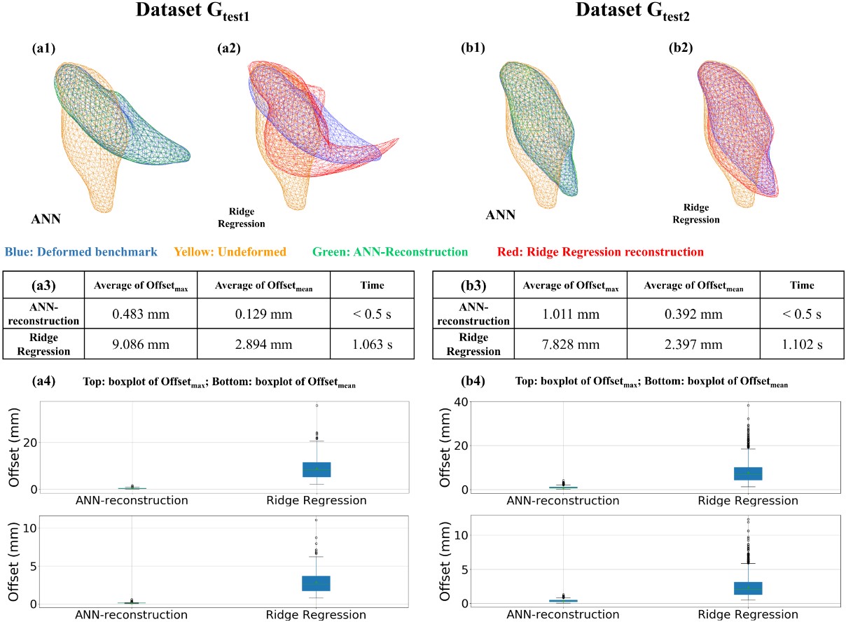
Figure 2: Reconstruction performance of our proposed approach and the Ridge Regression method on dataset $G_{test1}$ and $G_{test2}$, respectively. (a1), (a2), (b1), (b2) visualize the matching between the undeformed (reference) configuration (in yellow), the reconstructed deformed configuration (in green or red), and the corresponding benchmark deformed configuration (in blue). (a3) and (b3) show the average of $\mathrm{Offset_{max}}$ and $\mathrm{Offset_{mean}}$ of the two approaches on $G_{test1}$ and $G_{test2}$, respectively, the boxplots of which are separately represented in (a4) and (b4).

Following the strategy introduced in Section 2.5, we report reconstruction performances of the aforementioned methodologies for the H&N tumor model. The ANN is implemented with PyTorch 1.6.0, and all implementations demonstrated in this paper are completed using a consumer-grade CPU (4-core Intel I7-8550U @ 1.80GHz). Parametric studies are performed on ANN training and deformation reconstruction related parameters. Overall, the proposed approach enables fast and accurate deformation reconstruction of soft tissues and outperforms the method of ridge regression, the chosen baseline model in the paper.

3.1 Evaluation on deformation reconstruction performance

We evaluate the reconstruction performance of the proposed approach and the baseline model, respectively. For H&N tumor, $n_{d}=5$ FMs are chosen from the tetrahedral mesh according to the parameterization result. Figures 2(a1) and (b1) depict the comparison between the benchmark deformed configuration (in blue) and the ANN-reconstructed deformed configuration (in green) of a tested sample. Compared to the reconstruction results from the ridge regression (shown in Figures 2(a2) and (b2)), the reconstruction quality of the trained ANN is dramatically better than that of the baseline model; the boxplots of $\mathrm{Offset_{max}}$ and $\mathrm{Offset_{mean}}$ (shown in Figures 2(a4) and (b4)) also evidence this advantage of our proposed approach over the baseline method.

The average of $\mathrm{Offset_{max}}$ and $\mathrm{Offset_{mean}}$ as well as the reconstruction time of both methods on $G_{test1}$ and $G_{test2}$ are shown in Figure 2(a3) and (b3), respectively. It can be concluded that the predicted shapes generated from our proposed approach are very close ($1.5$% error compared to the tumor’s maximum dimension) to their corresponding benchmark deformed configurations; on an unseen dataset generated by a completely different force field generation strategy of the training dataset, the trained ANN still maintains a high reconstruction quality, demonstrating the approach’s robustness. In terms of the real time performance, our proposed approach generates deformed shapes within 0.5 s, which is markedly faster than the method of ridge regression and shows its capability of real-time reconstruction; the decrease of the baseline model’s reconstruction speed should account for the weights searching process, which is test-dataset-dependent and sensitive to the size of the dataset.

3.2 Parametric Studies

For the parametric study of the ANN architecture, we explore different hidden layer structures and conduct parameterization based on their reconstruction performances on $G_{test1}$. To reduce the time cost for ANN training as well as the workload of parameterization, we only evaluate combinations of two hidden layers ($[n_{1},n_{2}]$), each of which has a feasible neuron number list of 32, 64, 128 and 256 (resulting in a total of 16 possible combinations). Table 3 shows the results of the average of $\mathrm{Offset_{max}}$ and the elapsed time for training of all aforementioned architectures. Each of the architectures is trained three times, and the eventual result takes the average. Considering both the time efficiency of training process and the reconstruction quality, we choose the combination of [128, 64], which has relatively smallest average of $\mathrm{Offset_{max}}$ and moderate training time, as the optimal hidden layer structure.

Table 3: Parameterization results on ANN’s two-layer hidden structures $[n_{1},n_{2}]$.

$[n_{1},n_{2}]$	Average of $\mathrm{Offset_{max}}$ (mm)				Training time (s)
	32	64	128	256	32	64	128	256
32	0.590	0.538	0.544	0.574	747.285	732.081	788.877	1060.461
64	0.634	0.548	0.550	0.572	742.404	796.133	973.967	1244.056
128	0.893	0.533	0.539	0.575	815.583	1021.863	1255.345	1702.576
256	0.804	0.535	0.562	0.582	995.713	1255.417	1693.827	2668.229

We also conduct parametric studies on $n_{d}$ and $n_{w}$, the result of which are listed in Section A5. We select $n_{d}=5$ and $n_{w}=27$ in our implementation.

4 Conclusion

In this paper, a data-driven approach for predicting intraoperative soft tissue deformation based on FM registration is developed. The proposed approach incorporates both physically-based simulations and machine learning. For an H&N tumor model with maximum displacement of nearly $30$ mm, our approach is able to yield deformation predictions with sub-millimeter accuracy, which is the typical resolution of interventional ultrasound. Parametric studies on the number of FMs, number of PCs and ANN’s hidden layer architecture are performed to characterize the proposed prediction model. Further tests on models with various geometries and topologies have demonstrated the generality of our proposed approach. After the ANN is well trained, the deformation prediction of one case takes less than $0.5$ s, showing this work’s potential for real-time applications such as intraoperative tracking of soft tissues.

Broader Impact. The proposed approach can achieve real-time accurate deformation reconstruction of soft tissues. Although the pipeline is initial geometry dependent, it can still be utilized in patient-specific scenarios and assist surgeons to quickly reconstruct the deformed reconstruction by merely taking inputs from a few FMs. Overall, the presented study has demonstrated its potential to be clinically relevant.

Conflict of interests

Authors disclaim no conflict of interests.

Appendix

A1 Revised K-center clustering

Section 2.1 introduces the revised K-center clustering algorithm for FM searching. Algorithm 1 shows the pseudocode detailing the implementation of the aforementioned algorithm.

1

Input : Node set $V$, initial node $v_{0}$, number of centers $k$, minimal distance threshold $d_{min}$

Output : The list of all searched centers $V_{C}$

2 begin

3       Initialize $i\longleftarrow 0$, $V_{C}\longleftarrow\emptyset$, $S\longleftarrow\emptyset$; Add $v_{0}\longrightarrow V_{C}$;

4       while $i<k$ do

5             Set $maxAvg\longleftarrow 0$, $minVar\longleftarrow 1e5$, $v_{new}\longleftarrow\emptyset$;

6             foreach $v_{j}\in V$ do

7                   if $v_{j}\in V_{C}$ then

8                         Skip to the next loop;

9                        

10                  else

11                         $S\longleftarrow\emptyset$;

12                         foreach $c_{m}\in V_{C}$ do

13                               Compute euclidean distance between $v_{j}$ and $c_{m}$: $d_{m}=\mathrm{norm}(v_{j},c_{m})$;

14                               Add $d_{m}\longrightarrow S$;

15                              

16                         end foreach

17                        Compute average of $S$: $avg_{j}=\mathrm{avg}(S)$;

18                         Compute minimum of $S$: $min_{j}=\mathrm{min}(S)$;

19                        

20                        if $avg_{j}>maxAvg$ and $min_{j}>d_{min}$ then

21                               $v_{new}\longleftarrow v_{j}$;

22                               $maxAvg\longleftarrow avg_{j}$;

23                              

24                        else

25                               Skip to the next loop;

26                              

27                         end if

28                        

29                   end if

30                  

31             end foreach

32            Add $v_{new}\longrightarrow V_{C}$; Set $v_{new}\longleftarrow\emptyset$;

33             foreach $v_{n}\in V$ do

34                   if $v_{n}\in V_{C}$ then

35                         Skip to the next loop;

36                        

37                  else

38                         $S\longleftarrow\emptyset$;

39                         foreach $c_{p}\in V_{C}$ do

40                               Compute euclidean distance between $v_{n}$ and $c_{p}$: $d_{p}=\mathrm{norm}(v_{n},c_{p})$;

41                               Add $d_{p}\longrightarrow S$;

42                              

43                         end foreach

44                        Compute variance of $S$: $var_{n}=\mathrm{var}(S)$;

45                         Compute minimum of $S$: $min_{n}=\mathrm{min}(S)$;

46                        

47                        if $var_{n}<minVar$ and $min_{n}>d_{min}$ then

48                               $v_{new}\longleftarrow v_{n}$;

49                               $minVar\longleftarrow var_{n}$;

50                              

51                        else

52                               Skip to the next loop;

53                              

54                         end if

55                        

56                   end if

57                  

58             end foreach

59            Add $v_{new}\longrightarrow V_{C}$; $i\longleftarrow i+1$;

60            

61       end while

62      

63 end

64

Algorithm 1 Revised K-center clustering

The conventional K-center clustering algorithm iteratively searches the farthest point from the pre-obtained centers within a specific closed geometry [23]. To homogeneously distribute FMs in the target geometry, the revised K-center clustering algorithm simultaneously maximizes the average and minimizes the variance of distances among the selected centers. In this paper, the minimal distance threshold between two center points $d_{min}$ is set to 10 mm; two sub-loops are implemented in the algorithm to alternately obtain the point with the maximum distance average and the point with the minimum distance variance. With an initial point specified, the algorithm can automatically search the next best center point candidate based on the positions of pre-obtained centers and iteratively distribute the required number of center points within a closed mesh topology. Figure A1 shows FMs captured by the algorithm with different numbers of iterations (i.e. number of points $k$) within the H&N tumor model, evidencing that the revised K-center clustering algorithm enables the homogeneous distribution of FMs with arbitrarily specified $k$.

Figure A1: Distribution of different numbers ($k$s) of FMs in H&N tumor model. Starting at the initial node index of $97$, the red asterisks represent the centers obtained by the revised K-center clustering algorithm. $k=5$ is eventually selected for implementations in this paper.

A2 Introduction to modeling parameters and FEM nonlinearities

The H&N tumor studied in the paper is CT scanned and reconstructed using the commercial Synopsys’ Simpleware™ software and tetrahedralized in Netgen [24]. The parameters of modeling and property definitions of the used H&N model in this section are shown in Table A1.

Table A1: Parameters and material properties of the H&N tumor model.

Model Parameter	Symbol	H&N Tumor
Number of vertices	$n_{v}$	1158
Number of tetrahedral elements	$n_{e}$	8520
Number of vertices on the outer surface	$n_{s}$	760
Number of triangles on the outer surface	$n_{t}$	1516
Size	$dim_{x}\times dim_{y}\times dim_{z}$	$22~{}mm\times 39~{}mm\times 70~{}mm$
Fixed node indices (indexed from 1)	$V_{fix}$	[761, 1000, 1158]
Fiducial marker indices (indexed from 1)	$V_{FM}$	[97, 753, 1145, 5, 432]
Young’s modulus	$E$	$21~{}kPa$
Poisson’s ratio	$\upsilon$	$0.45$

With regard to the nonlinearity of FEM solver, we include the following nonlinearities in the process of dataset generation:

Material nonlinearity. We model the soft tissue as a neo-Hookean solid. Assuming the tissue is homogeneous, continuous and isotropic, the material constants can be computed based on its Young’s modulus and Poisson’s ratio following the strategy introduced in [25].

Geometric nonlinearity. By discretizing the simulation process, the force is divided into load increments which are gradually applied to the tumor. The transformation matrix and stiffness matrix must be recomputed at each simulation step to account for incremental changes in the geometry of the tumor.

Nonlinear element formulation. Each tetrahedral element has 10 nodes (4 of them at the element’s corners, 6 of them at the middle points of the element’ edges), each of which possesses 6 degrees of freedom (DOFs); a quadratic displacement function is defined for each tetrahedral element.

A3 Force field interpolation and test dataset generation

The deformation reconstruction performance is firstly demonstrated with $G_{test1}$, which is a sub-dataset generated when creating $G_{train}$. To further validate that the pre-trained ANN can predict the weights vector with a high quality on samples with different boundary conditions, we establish another test dataset $G_{test2}$, which is created based on a completely different force field settings. The pipeline to generate the force fields of $G_{test2}$ is as follows:

1. Randomly pick three nodes on the outer surface and assign a random concentrated force to each node. The scalar $\alpha$, which is used to control the magnitude of $f_{LBO}$, is applied here to control the value of each concentrated force;

2. Employ local Laplacian smoothing to each concentrated force to create a smoothed concentrated force field $f_{LSC}\in\mathbb{R}^{3n_{s}\times 1}$. In this paper, we specify the smoothing rate $\gamma=0.1$ and iteratively smooth in a total of 20 iterations. The effect of local force smoothing is shown in Figure A2(a);

3. Generate another LBO-reconstructed force field $f^{\prime}_{LBO}\in\mathbb{R}^{3n_{s}\times 1}$ (different from $f_{LBO}$ in Section 2.1) following the same strategy introduced in Section 2.1;

4. Generate a new force field $f_{interp}\in\mathbb{R}^{3n_{s}\times 1}$ by linear interpolating between $f^{\prime}_{LBO}$ and $f_{LSC}$ with an interpolation coefficient $\beta$. In this paper, 11 different $\beta$s are generated within the range of $[0,1]$ with an identical step size of 0.1. The results of force field interpolation is depicted in Figure A2(b).

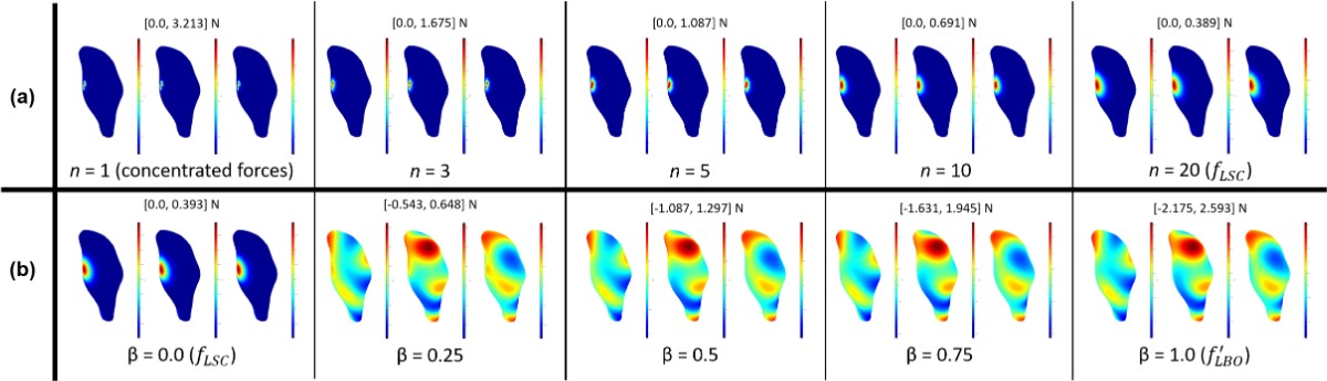
Figure A2: Visualization of the generating process of $f_{LSC}$ and $f_{interp}$ as well as some intermediate force fields on the H&N tumor. Row (a) depicts the process of Laplacian smoothing on three concentrated forces (in the figure, the initial magnitude of three forces: $[f_{x},f_{y},f_{z}]=[5.0,5.0,5.0]$ N), and $f_{LSC}$ is eventually obtained after 20 iterations of smoothing with $\gamma=0.1$. Row (b) shows linear interpolation results $f_{interp}$, which are used to construct $G_{test2}$, with different $\beta$s between $f_{LSC}$ ($\beta=0$) and $f^{\prime}_{LBO}$ ($\beta=1$).

A4 Additional results of deformation reconstruction performance

We provide more reconstruction results as well as some performance evaluation plots of our proposed approach here in addition to the representation in Section 3.1. Figure A3 shows the result of 12 samples constructed with different $\beta$s. From Figure A3(a), we can clearly observe that the majority of nodal mismatch results for each sample are under $1$ mm (corresponding to an error percentage of less than $1.5$% compared to the tumor’s maximum dimension of $70$ mm), demonstrating that the reconstruction performance of trained ANN with respect to different force field constructing parameters remains extraordinarily stable and outstanding. From the visualized results in Figure A3(b), we can conclude that the predicted shapes generated from our proposed approach are very close to the benchmark deformed configurations.

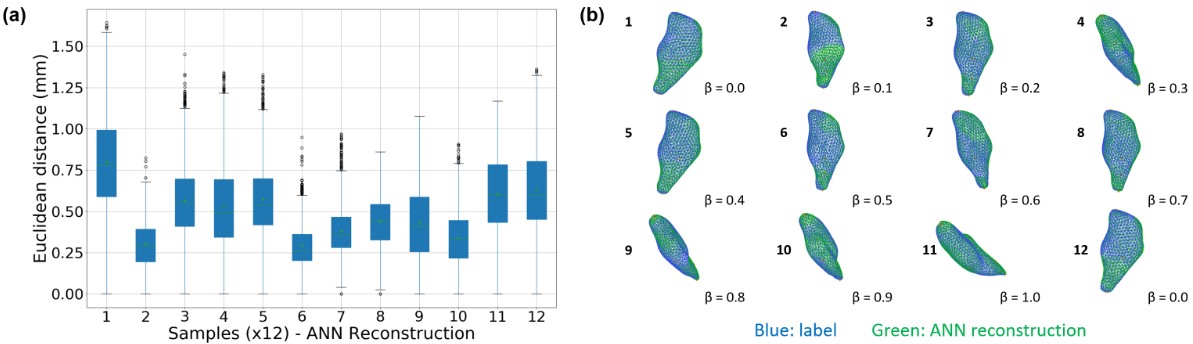
Figure A3: Reconstruction results of twelve samples with different force field interpolation coefficients ($\beta$s). (a) shows the nodal offsets distribution of each sample, the average nodal mismatch of which appears to be less than $1$ mm. (b) visualizes the matching between the benchmark deformed configurations (in blue) and reconstructed configurations of our proposed approach (in green).

Table A2: Reconstruction performance of the proposed approach with respect to $\beta$.

$\beta$	Average of $\mathrm{Offset_{max}}$ (mm)	Average of $\mathrm{Offset_{mean}}$ (mm)
$0$	1.181	0.452
$0.1$	1.085	0.415
$0.2$	1.016	0.383
$0.3$	0.941	0.370
$0.4$	0.932	0.366
$0.5$	0.889	0.350
$0.6$	0.903	0.356
$0.7$	0.971	0.378
$0.8$	0.951	0.379
$0.9$	1.089	0.413
$1$	1.167	0.453

Table A2 summarizes results of the reconstruction performance of sample groups with respect to different $\beta$s. For each group, the result is represented in the average of $\mathrm{Offset_{mean}}$ as well as the average of $\mathrm{Offset_{max}}$ of all samples. Results further validate the point that ANN trained on LBO-reconstructed dataset can perform very well on external unseen dataset with completely different force field modes. The relative lowest reconstruction error appears at $\beta=0.5$, the corresponding $f_{interp}$ at which has the minimal magnitude of force field and therefore the minimal magnitude of deformation. It is apparent that the smaller the deformation magnitude is, the better the reconstruction performance the ANN can achieve.

A5 Additional results of parametric studies

The number of principal components $n_{w}$ is selected as the minimum number of principal components required for the maximum nodal displacement error to be less than $1~{}mm$ when using PCA reconstruction. Figure A4 shows this error versus the number of PCs used in reconstruction. The displacement error is the average maximum error for 5-fold cross validation across the entire data set.

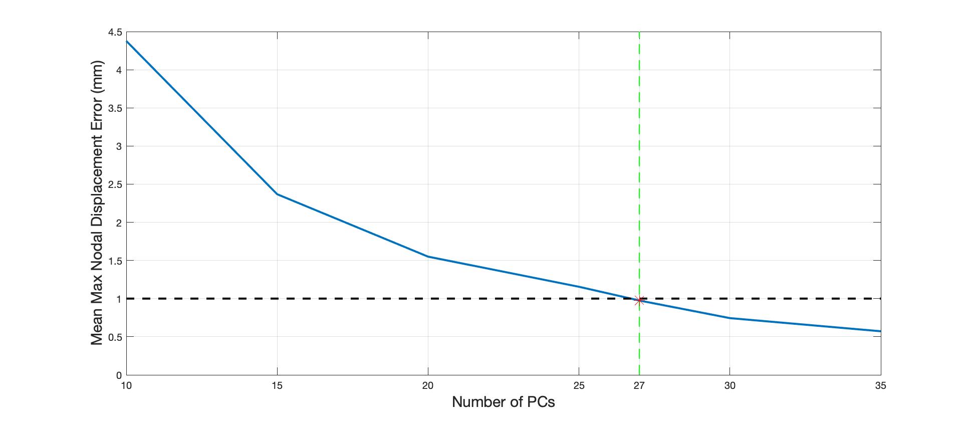
Figure A4: Maximum nodal displacement error across entire data set for varying number of principal components used during reconstruction.

The parametric study regarding $n_{d}$ is conducted on $G_{test1}$. Table A3 shows the parameterization results with respect to different $n_{d}$s ranging from 3 to 20. The results are reported in the average of $\mathrm{Offset_{mean}}$ and the average of $\mathrm{Offset_{max}}$ of all testing samples.

Table A3: Parameterization results w.r.t. $n_{d}$.

$n_{d}$	Average of $\mathrm{Offset_{max}}$ (mm)	Average of $\mathrm{Offset_{mean}}$ (mm)
$3$	2.205	0.634
$4$	1.587	0.593
$5$	0.837	0.287
$6$	0.729	0.241
$7$	0.675	0.228
$8$	0.641	0.217
$9$	0.590	0.203
$10$	0.485	0.176
$11$	0.452	0.167
$12$	0.458	0.168
$13$	0.412	0.159
$14$	0.440	0.162
$15$	0.392	0.148
$16$	0.386	0.144
$17$	0.402	0.153
$18$	0.352	0.136
$19$	0.365	0.141
$20$	0.302	0.113

Results of the aforementioned parametric studies show that with a few number of FMs and PCs, the pre-trained ANN can reconstruct the deformed configuration with a very high euclidean accuracy. With less number of FMs, it can be practically more convenient to track the displacements of a few points inside a soft tissue; with less number of PCs, the ANN enables a higher quality nonlinear mapping between the FM displacements and the weight vectors, which facilitates the learning process and benefits the speed and accuracy of deformation reconstruction.

References

- Azagury et al. [2015] Dan Elison Azagury, Monica M Dua, James C Barrese, Jaimie M Henderson, Nicolas C Buchs, Frederic Ris, Jordan M Cloyd, John B Martinie, Sharif Razzaque, Stéphane Nicolau, et al. Image-guided surgery. Current problems in surgery, 52(12):476–520, 2015.
- Zhang et al. [2017] Jinao Zhang, Yongmin Zhong, and Chengfan Gu. Deformable models for surgical simulation: a survey. IEEE reviews in biomedical engineering, 11:143–164, 2017.
- Carter et al. [2005] Timothy J Carter, Maxime Sermesant, David M Cash, Dean C Barratt, Christine Tanner, and David J Hawkes. Application of soft tissue modelling to image-guided surgery. Medical engineering & physics, 27(10):893–909, 2005.
- Lowe [2004] David G Lowe. Distinctive image features from scale-invariant keypoints. International journal of computer vision, 60(2):91–110, 2004.
- Cash et al. [2005] David M Cash, Michael I Miga, Tuhin K Sinha, Robert L Galloway, and William C Chapman. Compensating for intraoperative soft-tissue deformations using incomplete surface data and finite elements. IEEE transactions on medical imaging, 24(11):1479–1491, 2005.
- Rucker et al. [2013] D Caleb Rucker, Yifei Wu, Logan W Clements, Janet E Ondrake, Thomas S Pheiffer, Amber L Simpson, William R Jarnagin, and Michael I Miga. A mechanics-based nonrigid registration method for liver surgery using sparse intraoperative data. IEEE transactions on medical imaging, 33(1):147–158, 2013.
- Heiselman et al. [2017] Jon S Heiselman, Logan W Clements, Jarrod A Collins, Jared A Weis, Amber L Simpson, Sunil K Geevarghese, T Peter Kingham, William R Jarnagin, and Michael I Miga. Characterization and correction of intraoperative soft tissue deformation in image-guided laparoscopic liver surgery. Journal of Medical Imaging, 5(2):021203, 2017.
- Lunn et al. [2003] Karen E Lunn, Keith D Paulsen, David W Roberts, Francis E Kennedy, Alex Hartov, and Leah A Platenik. Nonrigid brain registration: synthesizing full volume deformation fields from model basis solutions constrained by partial volume intraoperative data. Computer Vision and Image Understanding, 89(2-3):299–317, 2003.
- Sun et al. [2014] Kay Sun, Thomas S Pheiffer, Amber L Simpson, Jared A Weis, Reid C Thompson, and Michael I Miga. Near real-time computer assisted surgery for brain shift correction using biomechanical models. IEEE journal of translational engineering in health and medicine, 2:1–13, 2014.
- Khallaghi et al. [2015] Siavash Khallaghi, C Antonio Sánchez, Abtin Rasoulian, Yue Sun, Farhad Imani, Amir Khojaste, Orcun Goksel, Cesare Romagnoli, Hamidreza Abdi, Silvia Chang, et al. Biomechanically constrained surface registration: Application to mr-trus fusion for prostate interventions. IEEE transactions on medical imaging, 34(11):2404–2414, 2015.
- Nimsky et al. [2001] Christopher Nimsky, Oliver Ganslandt, Peter Hastreiter, and Rudolf Fahlbusch. Intraoperative compensation for brain shift. Surgical neurology, 56(6):357–364, 2001.
- Monserrat et al. [2001] Carlos Monserrat, Ullrich Meier, M Alcaniz, Francisco Chinesta, and Mari C Juan. A new approach for the real-time simulation of tissue deformations in surgery simulation. Computer Methods and Programs in Biomedicine, 64(2):77–85, 2001.
- Zou et al. [2016] Yanni Zou, Peter X Liu, Qiangqiang Cheng, Pinhua Lai, and Chunquan Li. A new deformation model of biological tissue for surgery simulation. IEEE transactions on cybernetics, 47(11):3494–3503, 2016.
- Ling et al. [2014] Zhu Ling, Yu Ying, Zhang Baoquan, and Wang Lijing. An improved meshless method in virtual surgery simulation. In 2014 International Conference on Virtual Reality and Visualization, pages 449–454. IEEE, 2014.
- Jaradat et al. [2012] Mohammad A Jaradat, Muath N BaniSalim, and Fahed H Awad. Autonomous navigation robot for landmine detection applications. In 2012 8th International Symposium on Mechatronics and its Applications, pages 1–5. IEEE, 2012.
- Zhou et al. [2018] Jianyong Zhou, Zu Luo, Chunquan Li, and Mi Deng. Real-time deformation of human soft tissues: A radial basis meshless 3d model based on marquardt’s algorithm. Computer methods and programs in biomedicine, 153:237–252, 2018.
- Kyung et al. [2009] Ki-Uk Kyung, Jun-Young Lee, and Mandayam A Srinivasan. Precise manipulation of gui on a touch screen with haptic cues. In World Haptics 2009-Third Joint EuroHaptics conference and Symposium on Haptic Interfaces for Virtual Environment and Teleoperator Systems, pages 202–207. IEEE, 2009.
- Tonutti et al. [2017] Michele Tonutti, Gauthier Gras, and Guang-Zhong Yang. A machine learning approach for real-time modelling of tissue deformation in image-guided neurosurgery. Artificial intelligence in medicine, 80:39–47, 2017.
- Martínez-Martínez et al. [2017] Francisco Martínez-Martínez, María J Rupérez-Moreno, Marcelino Martínez-Sober, Juan Antonio Solves-Llorens, Delia Lorente, AJ Serrano-López, Sandra Martínez-Sanchis, C Monserrat, and José David Martín-Guerrero. A finite element-based machine learning approach for modeling the mechanical behavior of the breast tissues under compression in real-time. Computers in biology and medicine, 90:116–124, 2017.
- Morooka et al. [2008] Ken’ichi Morooka, Xian Chen, Ryo Kurazume, Seiichi Uchida, Kenji Hara, Yumi Iwashita, and Makoto Hashizume. Real-time nonlinear fem with neural network for simulating soft organ model deformation. In International Conference on Medical Image Computing and Computer-Assisted Intervention, pages 742–749. Springer, 2008.
- Mousavi et al. [2012] Seyed Reza Mousavi, Iman Khalaji, Ali Sadeghi Naini, Kaamran Raahemifar, and Abbas Samani. Statistical finite element method for real-time tissue mechanics analysis. Computer methods in biomechanics and biomedical engineering, 15(6):595–608, 2012.
- Yang et al. [2020] Humphrey Yang, Kuanren Qian, Haolin Liu, Yuxuan Yu, Jianzhe Gu, Matthew McGehee, Yongjie Jessica Zhang, and Lining Yao. Simulearn: Fast and accurate simulator to support morphing materials design and workflows. arXiv preprint arXiv:2007.15065, 2020.
- Park et al. [2014] Dohyung Park, Constantine Caramanis, and Sujay Sanghavi. Greedy subspace clustering. In Advances in neural information processing systems, pages 2753–2761, 2014.
- Schöberl [1997] Joachim Schöberl. Netgen an advancing front 2d/3d-mesh generator based on abstract rules. Computing and visualization in science, 1(1):41–52, 1997.
- Hu and Desai [2004] Tie Hu and Jaydev P Desai. Soft-tissue material properties under large deformation: Strain rate effect. In The 26th Annual International Conference of the IEEE Engineering in Medicine and Biology Society, volume 1, pages 2758–2761. IEEE, 2004.