Comprehensive analysis of beta decays
within and beyond the Standard Model

Abstract

Precision measurements in allowed nuclear beta decays and neutron decay are reviewed and analyzed both within the Standard Model and looking for new physics. The analysis incorporates the most recent experimental and theoretical developments. The results are interpreted in terms of Wilson coefficients describing the effective interactions between leptons and nucleons (or quarks) that are responsible for beta decay. New global fits are performed incorporating a comprehensive list of precision measurements in neutron decay, superallowed $0^{+}\rightarrow 0^{+}$ transitions, and other nuclear decays that include, for the first time, data from mirror beta transitions. The results confirm the $V$-$A$ character of the interaction and translate into updated values for $V_{ud}$ and $g_{A}$ at the $10^{-4}$ level. We also place new stringent limits on exotic couplings involving left-handed and right-handed neutrinos, which benefit significantly from the inclusion of mirror decays in the analysis.

1 Introduction

Precision measurements are essential ingredients in particle physics research. Their role is twofold. On the one hand, they allow us to extract numerical values of the free parameters of the Standard Model (SM), such as the gauge couplings or the Cabibbo-Kobayashi-Maskawa (CKM) matrix elements. On the other hand, they provide us with information about non-SM particles and their interactions, even if these particles are beyond reach of existing particle colliders.

Studies of beta decay processes are an important and active field within the precision program Cirigliano et al. (2013a); Naviliat-Cuncic and González-Alonso (2013); Vos et al. (2015); Gonzalez-Alonso et al. (2019). In the SM, beta decays are mediated by the exchange of a $W$ boson between light quark and lepton currents. Since the interaction strength between the $W$ and quarks in the SM is controlled by the CKM matrix, beta decays provide an opportunity to extract the $V_{ud}$ element of that matrix. In fact, this is currently the most precise (by far!) method to determine $V_{ud}$ Zyla et al. (2020).

Hypothetical particles such as $W^{\prime}$ bosons or leptoquarks may alter the rates and angular correlations of beta decays, as compared to the SM predictions. Rather than studying each such model successively, it is convenient to resort to effective field theory (EFT) techniques. In this approach, information about the underlying physics at high-energies that is relevant for beta decays is condensed into a small number of Wilson coefficients, which parametrize the strength of effective interactions between nucleons, electrons, and neutrinos at low energies. The general EFT Lagrangian describing these interactions at the leading order was written more than 60 years ago by Lee and Yang Lee and Yang (1956):

$${\mathcal{L}}_{\rm Lee-Yang} = -\bar{p}\gamma^{\mu}n\left(C_{V}\bar{e}\gamma_{\mu}\nu-C_{V}^{\prime}\bar{e}\gamma_{\mu}\gamma_{5}\nu\right)+\bar{p}\gamma^{\mu}\gamma_{5}n\left(C_{A}\bar{e}\gamma_{\mu}\gamma_{5}\nu-C_{A}^{\prime}\bar{e}\gamma_{\mu}\nu\right)$$ (1)

$$- \bar{p}n\left(C_{S}\bar{e}\nu-C_{S}^{\prime}\bar{e}\gamma_{5}\nu\right)-\frac{1}{2}\bar{p}\sigma^{\mu\nu}n\left(C_{T}\bar{e}\sigma_{\mu\nu}\nu-C_{T}^{\prime}\bar{e}\sigma_{\mu\nu}\gamma_{5}\nu\right)$$

$$- \bar{p}\gamma_{5}n\left(C_{P}\bar{e}\gamma_{5}\nu-C_{P}^{\prime}\bar{e}\nu\right)+{\rm h.c.}$$

Soon after that work, observables in beta decays were calculated in terms of the Wilson coefficients $C_{X}^{(^{\prime})}$ Jackson et al. (1957a); Ebel and Feldman (1957). This program led to the determination of the $V$-$A$ structure of the weak interaction, and it is currently used in searches for additional non-standard interactions. Along with refined experimental techniques and with careful calculations of small SM contributions, this program is strengthened by model-independent analyses of the data. The latter is the focus of this work, which is achieved through the construction of a likelihood function for the Wilson coefficients $C_{X}^{(^{\prime})}$. Given the likelihood, it is straightforward to extract information about any underlying high-energy theory - be it the SM or one of its extensions - once the map between $C_{X}^{(^{\prime})}$ and the high-energy parameters is established. The map can be calculated via the usual EFT techniques of matching at consecutive heavy particle thresholds, and renormalization group running in between thresholds (see e.g. Ref. Pich (1998)).

Although a number of global fits of beta decay data have been performed in the past Paul (1970); Boothroyd et al. (1984); Severijns et al. (2006); Gonzalez-Alonso et al. (2019), the complete likelihood function for the $C_{X}^{(^{\prime})}$, including all correlations, has never been constructed. Instead, only partial results are available, with selected Wilson coefficients simultaneously included in the fits. Such results have a limited value, since many theories beyond the SM generate an intricate pattern of Wilson coefficients, especially when the effect of mixing under renormalization group is taken into account. One of the goals of the present work is to implement a complete and model-independent EFT approach in the field of beta decays that includes the state-of-the art measurements and theoretical developments. We obtain a likelihood function for the Wilson coefficients in Eq. (1) while allowing all $C_{X}^{(^{\prime})}$ to be present at the same time, and taking into account all correlations.

In this analysis we use a comprehensive list of sensitive observables for allowed beta transitions, that is, the ones controlled by the Fermi and/or Gamow-Teller (GT) nuclear matrix elements. A key novelty of the present work is that we analyze, for the first time in a systematic and consistent fashion, the role of mirror beta decays in new physics searches. The name mirror refers to mixed Fermi-GT $J^{+}\!\!\!\to J^{+}$ transitions with isospin $T=1/2$ nuclei in both the initial and final states. Because of the high degree of theoretical control over the nuclear matrix elements, the importance of mirror decays for the precision program has long been recognized Severijns et al. (2008); Naviliat-Cuncic and Severijns (2009). In particular, they offer an alternative path to determining the $V_{ud}$ parameter Naviliat-Cuncic and Severijns (2009), which is subject to a vibrant experimental program for the determination of the relevant spectroscopic quantities and correlations. While the results are currently inferior in accuracy to $V_{ud}$ determinations from superallowed and neutron decays, they are affected by completely different systematic uncertainties, and thus they offer an important cross-check.

Another goal of this work is to analyze whether mirror transitions play a (numerically) important role in new physics searches. This is a reasonable possibility since the multi-dimensional parameter space of the Wilson coefficients in Eq. (1) is much larger than in the SM case. Indeed, we find that including mirror decays in the global fit leads to improvement of model-independent constraints on $C_{X}^{(^{\prime})}$ by approximately a factor of two. The results translate into stringent constraints on non-standard currents involving left- and right-handed neutrinos. We find that current data are well described by the SM. At the same time, the most general beyond-the-SM (BSM) fit shows a $3.2\sigma$ preference for non-standard tensor current interactions involving the right-handed neutrino. This tension is driven by a single recent measurement ($a_{n}$ by the aSPECT collaboration Beck et al. (2020)) and thus it should be taken with caution.

The structure of this article is the following. In Section 2 we review the theoretical formalism used for the quantitative description of mirror and other beta transitions. In Section 3 we describe the experimental results relevant for this analysis. Section 4 contains the main results: the confidence intervals for the Wilson coefficients of the effective Lagrangian in Eq. (1). We conclude in Section 5, and briefly discuss the prospect of improving the existing constraints by more precise measurements in mirror beta transitions.

2 Theoretical formalism

2.1 Lagrangian

At a fundamental level, nuclear beta decays probe charged-current interactions between the first generation of quarks and leptons. In this paper we adopt the EFT approach to parametrize these interactions. The central assumption is that, at the energy scale corresponding to beta decays, there is no other light degrees of freedom except for those of the SM and (eventually) the right-handed electron neutrino. Given this field content, the leading order effective Lagrangian at the scale $\mu\simeq 2$ GeV contains the following interactions relevant for beta decays

$${\mathcal{L}}\supset-\frac{V_{ud}}{v^{2}}\Big{[}\ \!\!\!\!\left(1+\epsilon_{L}\right)\ \bar{e}\gamma_{\mu}\nu_{L}\cdot\bar{u}\gamma^{\mu}(1-\gamma_{5})d\Big{.}~{}+~{}{\tilde{\epsilon}_{L}}\,\bar{e}\gamma_{\mu}\nu_{R}\cdot\bar{u}\gamma^{\mu}(1-\gamma_{5})d$$ (2)

$$+\epsilon_{R}\,\bar{e}\gamma_{\mu}\nu_{L}\cdot\bar{u}\gamma^{\mu}(1+\gamma_{5})d~{}+~{}{\tilde{\epsilon}_{R}}\,\bar{e}\gamma_{\mu}\nu_{R}\cdot\bar{u}\gamma^{\mu}(1+\gamma_{5})d$$

$$+{1\over 4}\epsilon_{T}\ \bar{e}\sigma_{\mu\nu}\nu_{L}\cdot\bar{u}\sigma^{\mu\nu}(1-\gamma_{5})d~{}+~{}\Big{.}{1\over 4}{\tilde{\epsilon}_{T}}\ \bar{e}\sigma_{\mu\nu}\nu_{R}\cdot\bar{u}\sigma^{\mu\nu}(1+\gamma_{5})d$$

$$+\epsilon_{S}\,\bar{e}\nu_{L}\cdot\bar{u}d~{}+~{}{\tilde{\epsilon}_{S}}\,\bar{e}\nu_{R}\cdot\bar{u}d-\epsilon_{P}\,\bar{e}\nu_{L}\cdot\bar{u}\gamma_{5}d~{}-~{}{\tilde{\epsilon}_{P}}\,\bar{e}\nu_{R}\cdot\bar{u}\gamma_{5}d\Big{]}+{\rm h.c.}~{}\qquad$$

where $u$, $d$, $e$ are the up quark, down quark, and electron fields, $\nu_{L,R}\equiv(1\pm\gamma_{5})\nu/2$ are the left-handed and right-handed electron neutrino fields, $V_{ud}$ is the $[\cdot]_{11}$ real entry of the unitary CKM matrix, and $v\approx 246.22$ GeV is related to the Fermi constant by $G_{F}=(\sqrt{2}v^{2})^{-1}$. We treat the neutrinos as massless. The Wilson coefficients $\epsilon_{X}$ and $\tilde{\epsilon}_{X}$, $X=L,R,S,P,T$, parametrize possible effects of non-SM particles, which have been integrated out. We assume, for concreteness, that all $\epsilon_{X}$ and $\tilde{\epsilon}_{X}$ are real, since the observables included in the analysis are not sensitive to their imaginary parts at the linear order in new physics. In the SM limit we have $\epsilon_{X}=\tilde{\epsilon}_{X}=0$ for all $X$. The situation where the right-handed neutrino is absent from the low-energy EFT (e.g. because it has a large Majorana mass) can be described by setting $\tilde{\epsilon}_{X}=0$ for all $X$.

The quark-level Lagrangian in Eq. (2) is what matters in particle physics. Its parameters can be readily related to masses and couplings of specific BSM models, or to Wilson coefficients of a more fundamental EFT above the electroweak scale. However, the momentum exchange in beta decays is far below the QCD scale, and thus we need to connect the quark-level Lagrangian above with the nucleon-level Lee-Yang Lagrangian in Eq. (1), which can be rewritten in the following form:

$${\mathcal{L}}_{\rm Lee-Yang} = -\bar{p}\gamma^{\mu}n\left(C_{V}^{+}\bar{e}\gamma_{\mu}\nu_{L}+C_{V}^{-}\bar{e}\gamma_{\mu}\nu_{R}\right)-\bar{p}\gamma^{\mu}\gamma_{5}n\left(C_{A}^{+}\bar{e}\gamma_{\mu}\nu_{L}-C_{A}^{-}\bar{e}\gamma_{\mu}\nu_{R}\right)$$ (3)

$$- \bar{p}n\left(C_{S}^{+}\bar{e}\nu_{L}+C_{S}^{-}\bar{e}\nu_{R}\right)-\frac{1}{2}\bar{p}\sigma^{\mu\nu}n\left(C_{T}^{+}\bar{e}\sigma_{\mu\nu}\nu_{L}+C_{T}^{-}\bar{e}\sigma_{\mu\nu}\nu_{R}\right)$$

$$+ \bar{p}\gamma_{5}n\left(C_{P}^{+}\bar{e}\nu_{L}-C_{P}^{-}\bar{e}\nu_{R}\right)+{\rm h.c.}$$

after a simple change of variables $C_{X}=(C_{X}^{+}+C_{X}^{-})/2$, $C_{X}^{\prime}=(C_{X}^{+}-C_{X}^{-})/2$ that separates the left-handed (via $C_{X}^{+}$) and right-handed (via $C_{X}^{-}$) neutrino couplings, which affect the nuclear observables in a different way due to the fact that only the former may interfere with the SM amplitudes. Consequently, in the $C_{X}^{\pm}$ variables the experimental constraints are physically more transparent, and the matching to the quark-level Lagrangian is more straightforward. At a more practical level, correlations in the global fit are hugely reduced when using the $C_{X}^{\pm}$ variables. The relation between the parameters in Eq. (2) and in Eq. (3) is given by Gonzalez-Alonso et al. (2019)

$$C_{V}^{+} = {V_{ud}\over v^{2}}g_{V}\sqrt{1+\Delta_{R}^{V}}\big{(}1+\epsilon_{L}+\epsilon_{R}\big{)},\qquad C_{V}^{-}={V_{ud}\over v^{2}}g_{V}\sqrt{1+\Delta_{R}^{V}}\big{(}\tilde{\epsilon}_{L}+\tilde{\epsilon}_{R}\big{)},$$

$$C_{A}^{+} = -{V_{ud}\over v^{2}}g_{A}\sqrt{1+\Delta_{R}^{A}}\big{(}1+\epsilon_{L}-\epsilon_{R}\big{)},\qquad C_{A}^{-}={V_{ud}\over v^{2}}g_{A}\sqrt{1+\Delta_{R}^{A}}\big{(}\tilde{\epsilon}_{L}-\tilde{\epsilon}_{R}\big{)},$$

$$C_{T}^{+} = {V_{ud}\over v^{2}}g_{T}\epsilon_{T},\qquad C_{T}^{-}={V_{ud}\over v^{2}}g_{T}\tilde{\epsilon}_{T},$$

$$C_{S}^{+} = {V_{ud}\over v^{2}}g_{S}\epsilon_{S},\qquad C_{S}^{-}={V_{ud}\over v^{2}}g_{S}\tilde{\epsilon}_{S},$$

$$C_{P}^{+} = {V_{ud}\over v^{2}}g_{P}\epsilon_{P},\qquad C_{P}^{-}=-{V_{ud}\over v^{2}}g_{P}\tilde{\epsilon}_{P},$$ (4)

where $g_{V,A,S,P,T}$ are vector, axial, scalar, pseudoscalar, and tensor charges of the nucleon Herczeg (2001); Gonzalez-Alonso et al. (2019), which must be determined using lattice or other theoretical techniques. For the vector charge, one can prove that $g_{V}=1$ up to (negligible) quadratic corrections in isospin-symmetry breaking Ademollo and Gatto (1964). We will use the FLAG’19 averages Aoki et al. (2020) for the axial, scalar and tensor charges: $g_{A}=1.251(33)$, $g_{S}=1.022(100)$ and $g_{T}=0.989(33)$ Chang et al. (2018); Gupta et al. (2018) (see also Ref. Gonzalez-Alonso and Martin Camalich (2014)). Although the pseudoscalar charge is enhanced by the pion pole, namely $g_{P}=349(9)$ Gonzalez-Alonso and Martin Camalich (2014), the suppression of the pseudoscalar contributions to the observables is larger and they will be neglected in the following.

The matching in Eq. (2.1) includes the short-distance (inner) radiative corrections $\Delta_{R}^{V}$ and $\Delta_{R}^{A}$. Especially the former is important, because it is necessary to extract $V_{ud}$ from nuclear data. Four recent calculations of this quantity are available Seng et al. (2018); Czarnecki et al. (2019); Seng et al. (2020); Hayen (2021), all within $1\sigma$. In this analysis we use the Seng et al. evaluation, $\Delta_{R}^{V}=0.02467(22)$ Seng et al. (2018), which has the smallest uncertainty. We will discuss the impact of this choice. Given the assumption about the reality of $\epsilon_{X}$ and $\tilde{\epsilon}_{X}$, all $C_{X}^{\pm}$ are then also real.

At leading order, nuclear effects are encapsulated in the so-called Fermi and GT matrix elements, $M_{F,GT}$. Leading-order expressions for beta decay observables in terms of the Lee-Yang Wilson coefficients $C_{X}^{\pm}$ can be found in Refs. Jackson et al. (1957b); Ebel and Feldman (1957). However, given the experimental precision, subleading effects such as weak-magnetism and long-distance electromagnetic corrections have to be included in the SM terms. These small contributions can be calculated with large accuracy for the transitions that are included in this work Holstein (1974); Cirigliano et al. (2013a); Hayen et al. (2018); Hayen and Young (2020).

The main results of this work are the constraints on the $C_{X}^{\pm}$ Wilson coefficients using neutron and nuclear physics data, with special attention to the role played by mirror beta decays which are included in a global fit for the first time. In the remainder of this section we review how beta decay observables included in this work depend on the $C_{X}^{\pm}$ Wilson coefficients.

2.2 Ft values and neutron lifetime

The total decay width of an allowed beta transition can be calculated from the formula

$$\Gamma_{i}=\big{(}1+\delta_{i}\big{)}{M_{F}^{2}m_{e}^{5}\over 4\pi^{3}}f^{i}_{V}\hat{\xi}_{i}\bigg{[}1+\gamma_{i}b_{i}\bigg{\langle}{m_{e}\over E_{e}}\bigg{\rangle}_{i}\bigg{]}\,.$$ (5)

The index $i$ labels transition-dependent quantities. Radiative corrections, other than the short-distance ones already included in $\Delta_{R}^{V,A}$, are encoded in $\delta_{i}$. They are customarily split as $1+\delta_{i}=(1+\delta_{R}^{\prime})(1+\delta_{NS}^{V}-\delta_{C}^{V})$, where $\delta_{R}^{\prime}$ is the dominant piece of the long-distance (outer) radiative corrections that depends trivially (only via $Z$ and $\Delta$) on the nucleus, $\delta_{NS}^{V}$ is the nuclear-structure-dependent piece, and $\delta_{C}^{V}$ is the isospin-symmetry breaking correction. $M_{F}$ is the Fermi matrix element in the isospin limit, which for a transition between two members of the same isospin multiplet is given by $M_{F}=\sqrt{j(j+1)-m(m\pm 1)}$, where $(j,m)$ are the isospin quantum numbers of the parent nucleus, The factor $f^{i}_{V}$ is the phase space integral given by

$$f^{i}_{V}={1\over m_{e}^{5}}\int_{m_{e}}^{\Delta_{i}}dE_{e}F_{i}(\Delta_{i}-E_{e})^{2}p_{e}E_{e},$$ (6)

where $m_{e}$ is the electron mass, $p_{e}=\sqrt{E_{e}^{2}-m_{e}^{2}}$, $\Delta_{i}$ is the maximal total energy of the beta particle, and $F_{i}\equiv 4(2p_{e}\,R_{i})^{2(\gamma_{i}-1)}e^{\pi\eta_{i}}{|\Gamma(\gamma_{i}+i\eta_{i})|^{2}/\Gamma(1+2\gamma_{i})^{2}}$ is the Fermi function describing the Coulomb corrections, with $\gamma_{i}\equiv\sqrt{1-(\alpha Z_{i})^{2}}$, $Z_{i}$ ($R_{i}$) the charge (radius) of the daughter nucleus, $\alpha$ the electromagnetic structure constant, and $\eta_{i}\equiv\pm{\alpha Z_{i}E_{e}/p_{e}}$. Above and in all of the following, the upper (lower) sign applies to $\beta^{-}$ ($\beta^{+}$) transitions. Further details about subleading corrections that have to be included in $f^{i}_{V}$ are discussed in Refs. Hardy and Towner (2005); Hayen et al. (2018). The second term in the square bracket in Eq. (5) is called the Fierz term. It is proportional to the weighted average of the electron mass over its energy:

$$\bigg{\langle}{m_{e}\over E_{e}}\bigg{\rangle}_{i}\equiv{\int_{m_{e}}^{\Delta_{i}}dE_{e}F_{i}(\Delta_{i}-E_{e})^{2}p_{e}m_{e}\over\int_{m_{e}}^{\Delta_{i}}dE_{e}F_{i}(\Delta_{i}-E_{e})^{2}p_{e}E_{e}}.$$ (7)

The dependence of the decay width on the Wilson coefficients of the Lee-Yang Lagrangian enters via the combinations $\hat{\xi}_{i}$ and $b_{i}$ defined as

$$\hat{\xi}_{i} \equiv (C_{V}^{+})^{2}+(C_{S}^{+})^{2}+(C_{V}^{-})^{2}+(C_{S}^{-})^{2}+{f_{A}^{i}\over f_{V}^{i}}{(C_{V}^{+})^{2}\over(C_{A}^{+})^{2}}\tilde{\rho}_{i}^{2}\bigg{[}(C_{A}^{+})^{2}+(C_{T}^{+})^{2}+(C_{A}^{-})^{2}+(C_{T}^{-})^{2}\bigg{]},$$

$$b_{i}\hat{\xi}_{i} \equiv \pm 2\bigg{\{}C_{V}^{+}C_{S}^{+}+C_{V}^{-}C_{S}^{-}+{(C_{V}^{+})^{2}\over(C_{A}^{+})^{2}}\tilde{\rho}_{i}^{2}\bigg{[}C_{A}^{+}C_{T}^{+}+C_{A}^{-}C_{T}^{-}\bigg{]}\bigg{\}},$$ (8)

where the factors $f_{A}^{i}/f_{V}^{i}$ encode corrections to the (axial-vector) phase space integral. For the mirror transitions relevant to our analysis, $f_{A}^{i}/f_{V}^{i}$ can be estimated by theoretical methods, and have values close to unity Hayen and Severijns (2019). The “polluted” mixing ratio $\tilde{\rho}_{i}$ in Eq. (2.2) is defined as

$$\tilde{\rho}_{i}={C_{A}^{+}\over C_{V}^{+}}{M_{\rm GT}\over M_{\rm F}}{\big{(}1+\delta^{A}_{\rm NS}-\delta^{A}_{\rm C}\big{)}^{1/2}\over\big{(}1+\delta^{V}_{\rm NS}-\delta^{V}_{\rm C}\big{)}^{1/2}}~{},$$ (9)

where $M_{\rm GT}/M_{\rm F}$ is the ratio between the GT and Fermi matrix elements in the isospin limit, and $\delta^{A}_{\rm NS}$, $\delta^{A}_{\rm C}$ are the axial-vector equivalents to $\delta^{V}_{\rm NS}$, $\delta^{V}_{\rm C}$ mentioned earlier. Using Eq. (2.1) to re-express $C_{A}^{+}/C_{V}^{+}$ one can see that, in the SM limit, $\tilde{\rho}_{i}$ reduces to the usual mixing ratio $\rho_{i}$ defined in Refs. Severijns et al. (2008); Naviliat-Cuncic and Severijns (2009). However, in the presence of new physics, $\tilde{\rho}_{i}$ depends on unknown parameters $\epsilon_{L,R}$, and it is not anymore a pure QCD/nuclear quantity. In practice, the distinction between $\rho_{i}$ and $\tilde{\rho}_{i}$ is not relevant because the mixing ratios $\rho_{i}$ cannot be calculated with sufficient precision by current theoretical techniques for nuclei with $A>1$. Thus, the mixing ratios, whether $\rho_{i}$ or $\tilde{\rho}_{i}$, have to be treated as free parameters in the fits, together with $C_{X}^{\pm}$.

Rather than the observable decay width, experimental groups or theory compilations often communicate the corrected half-life ${\cal F}t$ defined as

$${\cal F}t_{i}\equiv{f^{i}_{V}(1+\delta_{i})\log 2\over\Gamma_{i}}={4\pi^{3}\log 2\over M_{F}^{2}m_{e}^{5}}\bigg{[}\hat{\xi}_{i}+\gamma_{i}b_{i}\hat{\xi}_{i}\bigg{\langle}{m_{e}\over E_{e}}\bigg{\rangle}_{i}\bigg{]}^{-1}.$$ (10)

For the superallowed ($0^{+}\to 0^{+}$, $j=1$) beta decays, one has $M_{F}=\sqrt{2}$ and $\rho=0$ in Eq. (10) and Eq. (2.2). In the SM limit, ${\cal F}t$ is predicted to be universal for all superallowed transitions. However, beyond the SM one can have $b_{i}\neq 0$ and then ${\cal F}t$ depends on the transition via the Fierz factor $b_{i}\langle m_{e}/E_{e}\rangle_{i}$. For mirror ($J^{+}\to J^{+}$, $j=1/2$) beta decays one has $M_{F}=1$, and ${\cal F}t_{i}$ is a function (via $\hat{\xi}_{i}$ and $b_{i}$) of the transition-dependent mixing ratio $\rho_{i}$. Consequently, for mirror decays ${\cal F}t_{i}$ is transition dependent even in the SM limit. For neutron decay one has $M_{F}=1$ and $\rho_{n}=-\sqrt{3}g_{A}$, up to ${\cal O}(0.2\%)$ radiative corrections Hayen (2021). Rather than the corrected half-life ${\cal F}t$, experiments customarily quote the neutron lifetime:

$$\tau_{n}\equiv{1\over\Gamma_{n}}={4\pi^{3}\over(1+\delta_{n})m_{e}^{5}f_{n}}\bigg{[}\hat{\xi}_{n}+\gamma_{n}b_{n}\hat{\xi}_{n}\bigg{\langle}{m_{e}\over E_{e}}\bigg{\rangle}_{n}\bigg{]}^{-1}~{}.$$ (11)

We use here $f_{n}=1.6887(1)$ Czarnecki et al. (2018) and $\delta_{n}=\delta_{R}^{\prime}{}^{n}=0.014902(2)$ Towner and Hardy (2010), and ignore the negligible Wilkinson (1982) correction due to $f_{A}^{n}/f_{V}^{n}$ in Eq. (2.2).

2.3 Correlation measurements

The lifetime measurements discussed in the previous subsection probe only a limited number of combinations of the Lee-Yang Wilson coefficients and the mixing ratios. To avoid degeneracy in a global fit, one needs to include a wider palette of observables. Nuclear experiments measure various angular correlations between the decay products. Assuming CP conservation and summing over polarizations of the daughter nucleus and $\beta$ particle, the differential decay width can be cast in the form

$${d\Gamma_{i}\over dE_{e}d{\Omega_{e}}d{\Omega_{\nu}}} = \hat{\xi}_{i}{M_{F}^{2}\over 64\pi^{5}}F_{i}(\Delta_{i}-E_{e})^{2}p_{e}E_{e}\bigg{\{}1+b_{i}{m_{e}\over E_{e}}+a_{i}{\vec{p}_{e}\over E_{e}}\cdot{\vec{p}_{\nu}\over E_{\nu}}+A_{i}{\vec{p}_{e}\over E_{e}}\cdot{\langle\vec{J}\rangle\over J}+B_{i}{\vec{p}_{\nu}\over E_{\nu}}\cdot{\langle\vec{J}\rangle\over J}$$ (12)

$$+ c_{i}\bigg{[}{\vec{p}_{e}\cdot\vec{p}_{\nu}\over 3E_{e}E_{\nu}}-{(\vec{p}_{e}\cdot\vec{j})(\vec{p}_{\nu}\cdot\vec{j})\over E_{e}E_{\nu}}\bigg{]}\bigg{[}{J(J+1)-3(\langle\vec{J}\rangle\cdot\vec{j})^{2}\over J(2J-1)}\bigg{]}\bigg{\}}~{},$$

where the indices $e$ and $\nu$ refer to the $\beta$ particle and neutrino, respectively and the symbols $\Omega$, $\vec{p}$ and $E$ denote the angular coordinates, momentum and energy of the leptons, $\langle\vec{J}\rangle$ is the polarization of the parent nucleus, $J$ is its spin, and $\vec{j}$ is the unit vector in the polarization direction. Since no experiment measures the coefficient $c_{i}$, we will not discuss it in the following. The remaining parameters in Eq. (12) are referred to as the $\beta$-$\nu$ correlation ($a$), the $\beta$-asymmetry ($A$), and the neutrino asymmetry ($B$). For a mixed Fermi and GT $\beta$ transition they can be expressed by the Lee-Yang Wilson coefficients as

$$\hat{\xi}_{i}a_{i} = (C_{V}^{+})^{2}-(C_{S}^{+})^{2}+(C_{V}^{-})^{2}-(C_{S}^{-})^{2}-{\tilde{\rho}_{i}^{2}\over 3}{(C_{V}^{+})^{2}\over(C_{A}^{+})^{2}}\bigg{[}(C_{A}^{+})^{2}-(C_{T}^{+})^{2}+(C_{A}^{-})^{2}-(C_{T}^{-})^{2}\bigg{]},$$

$$\hat{\xi}_{i}A_{i} = -2\tilde{\rho}_{i}{C_{V}^{+}\over C_{A}^{+}}\sqrt{J\over J+1}\bigg{\{}C_{V}^{+}C_{A}^{+}-C_{S}^{+}C_{T}^{+}-C_{V}^{-}C_{A}^{-}+C_{S}^{-}C_{T}^{-}\bigg{\}}$$

$$\mp{\tilde{\rho}_{i}^{2}\over J+1}{(C_{V}^{+})^{2}\over(C_{A}^{+})^{2}}\bigg{\{}(C_{A}^{+})^{2}-(C_{T}^{+})^{2}-(C_{A}^{-})^{2}+(C_{T}^{-})^{2}\bigg{\}},$$

$$\hat{\xi}_{i}B_{i} = -2\tilde{\rho}_{i}{C_{V}^{+}\over C_{A}^{+}}\sqrt{J\over J+1}\bigg{\{}C_{V}^{+}C_{A}^{+}+C_{S}^{+}C_{T}^{+}-C_{V}^{-}C_{A}^{-}-C_{S}^{-}C_{T}^{-}$$

$$\pm{m_{e}\over E_{e}}\left[C_{S}^{+}C_{A}^{+}+C_{V}^{+}C_{T}^{+}-C_{S}^{-}C_{A}^{-}-C_{V}^{-}C_{T}^{-}\right]\bigg{\}}$$

$$\pm{\tilde{\rho}_{i}^{2}\over J+1}{(C_{V}^{+})^{2}\over(C_{A}^{+})^{2}}\bigg{\{}(C_{A}^{+})^{2}+(C_{T}^{+})^{2}-(C_{A}^{-})^{2}-(C_{T}^{-})^{2}\pm{2m_{e}\over E_{e}}\bigg{[}C_{A}^{+}C_{T}^{+}-C_{A}^{-}C_{T}^{-}\bigg{]}\bigg{\}}.$$

We also define the tilde correlation coefficients as

$$\tilde{X}_{i}\equiv{X_{i}\over 1+b_{i}\big{\langle}{m_{e}/E_{e}}\big{\rangle}_{i}},\qquad\tilde{X}_{i}(E_{e})\equiv{X_{i}\over 1+b_{i}{m_{e}/E_{e}}},\qquad X=a,A,B~{},$$ (14)

which are the quantities that can be determined from asymmetries (integrated over energies and for a fixed-energy respectively) Gonzalez-Alonso and Naviliat-Cuncic (2016). The distinction between the $\tilde{X}_{i}$ and $X_{i}$ correlations is only relevant beyond the SM, when the Fierz term is non-zero. Many experimental results in the literature do not make this distinction explicit, because they operate under the SM hypothesis. Some care is needed when interpreting such results Gonzalez-Alonso and Naviliat-Cuncic (2016). We discuss this issue in more detail in the following section.

For completeness, in Appendix A we collect the expressions for other observables used in the present analysis: the ratio between longitudinal polarization of $\beta$ particles from Fermi and Gamow-Teller transitions and the correlation coefficients $a$ and $A$ in pure Gamow-Teller decays.

3 Experimental data

3.1 Mirror beta decays

The ${\cal F}t$ values have been extracted quite precisely for numerous mirror transitions from the measured lifetimes, branching ratios and $Q$-values and calculated $\delta_{i}$ corrections Severijns et al. (2008). However, those alone do not provide any information about the fundamental SM parameters or new physics contributions, because the decay rates also depend on the mixing ratio $\tilde{\rho}_{i}$ (see Eq. (5) and Eq. (2.2)) which cannot be currently calculated from first principles with high precision. But when both ${\cal F}t$ and some correlation coefficient are determined for a given transition, then $V_{ud}$ and the BSM coefficients can be probed. The dependence of observables on the Wilson coefficients $C_{X}^{\pm}$ is a function of the transition-dependent $\tilde{\rho}_{i}$ and nuclear spin $J$, thus each mirror transition probes a distinct combination of $C_{X}^{\pm}$. This results in a strong interplay between different transitions, especially regarding the constraints on $C_{X}^{\pm}$ in the presence of new physics.

There are currently six mirror transitions for which precise spectroscopic measurements exist to extract the ${\cal F}t$ values as well as measurements of a correlation coefficient. These are summarized in Table 1 and they are a crucial experimental input for the fits carried out in this work.

Since some of the measurements have a precision at the level of $1\%$ or below, linear recoil effects (mainly weak magnetism) have to be considered Holstein (1974). We follow the same prescription as in Ref. Naviliat-Cuncic and Severijns (2009) to take into account its contribution to the asymmetries in ¹⁹Ne, ²¹Na, and ³⁵Ar. We use updated values for the nuclear magnetic moments from Ref. IAEA-database , though these changes do not have any impact in the analysis. For ³⁷K, we do not include recoil effects because they were already subtracted from the value of $A$ in Ref. Fenker et al. (2018). Finally for ¹⁷F and ²⁹P we neglect all subleading contributions because the experimental uncertainty is much larger for these transitions.

Other changes with respect to the experimental input used in the SM analyses carried out in Refs. Severijns et al. (2008); Naviliat-Cuncic and Severijns (2009) are the following:

• To allow for non-standard interactions, we reinterpret the extractions of $A$ and $B$ through the usual tilde prescription, Eq. (14). The $a$ extraction in Ref. Vetter et al. (2008) is more complicated. In principle the tilde prescription is not valid because the correlation is not extracted from an asymmetry measurement and thus the data should have been analyzed using two independent free parameters $a$ and $b$ Gonzalez-Alonso and Naviliat-Cuncic (2016). However, we have checked that, under the conditions of this measurement, the time of flight distribution is mainly sensitive to a specific combination of $a$ and $b$ that happens to be well approximated by $\tilde{a}$.

• The $f_{A}/f_{V}$ values are taken from Refs. Hayen (2021, ), where a small double-counting affecting previous values was pointed out and resolved. These corrections are all below $0.15\%$. Their uncertainties are very small and can be neglected in our analysis.

• The analysis in Ref. Naviliat-Cuncic and Severijns (2009) included the measurement of the neutrino asymmetry ${B}_{\nu}$ in ³⁷K decay, which has a relative uncertainty of 3.1% Melconian et al. (2007). We include here as well the recent precise measurement of $\tilde{A}$ from Ref. Fenker et al. (2018). This $\beta$-asymmetry parameter has the smallest relative uncertainty from all mirror transitions.

• We include the recent result of Ref. Combs et al. (2020) for the beta asymmetry in ¹⁹Ne.

• The results from Ref. Naviliat-Cuncic and Severijns (2009) have motivated several measurements of branching ratios, lifetimes and $Q$-values for the extraction of ${\cal F}t$ values Shidling et al. (2014); Rebeiro et al. (2019); Karthein et al. (2019). The review of spectroscopic data is not within the scope of the present analysis. The ${\cal F}t$ values adopted here are indicated in Table 1.

• For completeness, for all these $\beta^{+}$ transitions, we update the maximal total energies $\Delta=Q_{\rm EC}-m_{e}$, using the transition energies $Q_{\rm EC}$ given in the 2016 Atomic Mass Evaluation (AME) Database Wang et al. (2017), except for ²¹Na for which we use a newer measurement Karthein et al. (2019).

Parent	Spin	$\Delta$ [MeV]	$\langle m_{e}/E_{e}\rangle$	$f_{A}/f_{V}$	${\cal F}t$ [s]	Correlation
17F	5/2	2.24947(25)	0.447	1.0007(1)	2292.4(2.7) Brodeur et al. (2016)	$\tilde{A}=0.960(82)$ Severijns et al. (1989, 2006)
19Ne	1/2	2.72849(16)	0.386	1.0012(2)	1721.44(92) Rebeiro et al. (2019)	$\tilde{A}_{0}=-0.0391(14)$ Calaprice et al. (1975)
						$\tilde{A}_{0}=-0.03871(91)$ Combs et al. (2020)
21Na	3/2	3.035920(18)	0.355	1.0019(4)	4071(4) Karthein et al. (2019)	$\tilde{a}=0.5502(60)$ Vetter et al. (2008)
29P	1/2	4.4312(4)	0.258	0.9992(1)	4764.6(7.9) Long et al. (2020)	$\tilde{A}=0.681(86)$ Masson and Quin (1990)
35Ar	3/2	5.4552(7)	0.215	0.9930(14)	5688.6(7.2) Severijns et al. (2008)	$\tilde{A}=0.430(22)$ Garnett et al. (1988); Converse et al. (1993); Naviliat-Cuncic and Severijns (2009)
37K	3/2	5.63647(23)	0.209	0.9957(9)	4605.4(8.2) Shidling et al. (2014)	$\tilde{A}=-0.5707(19)$ Fenker et al. (2018)
						$\tilde{B}=-0.755(24)$ Melconian et al. (2007)

Table 1: Mirror beta decays used in this analysis. The quantity $\langle m_{e}/E_{e}\rangle$ is calculated via Eq. (7), using the endpoint energy listed in the table. The latter are taken from AME2016 Wang et al. (2017), except that of ²¹Na Karthein et al. (2019). The values of $f_{A}/f_{V}$ come from Ref. Hayen and Severijns (2019); Hayen . We also used the notation $\tilde{A}_{0}\equiv\tilde{A}(m_{e})$.

The measurement of the total $\beta$-asymmetry (i.e. the asymmetry integrated over the energy of the beta particle) only gives us access to $\tilde{A}$. However, it is clear that measuring the energy dependence of the $\beta$-asymmetry makes possible to extract separately $A$ and the Fierz term $b$, cf. Eq. (14). We encourage experimental groups to carry out such analyses in order to extract all the information contained in the data. Such measurements of the $\beta$-asymmetry as a function of the energy have already been performed, see e.g. Refs. Fenker et al. (2018); Combs et al. (2020), but not analyzed with a two-parameter fit.

3.2 Fermi, Gamow-Teller and neutron decays

For pure Fermi, pure GT, and neutron decay, we use the same data set included in the global fit of Ref. Gonzalez-Alonso et al. (2019) (total rates and asymmetries) with some updates that we explain in this section. The complete list of observables and references is collected in Appendix B.

The measurement of the $\beta$-asymmetry in neutron decay by the PERKEO-III collaboration Markisch et al. (2019) represents a major change, not only because it is the most precise to date, but also because after its inclusion in the global data set and using the PDG criteria for averaging various measurements Zyla et al. (2020), the scale factor $S$ inflating the error has decreased considerably. The numerical change is very significant:

$$\tilde{A}_{n} = -0.11869(99)~{}\text{($S=2.6$, pre PERKEO-III)}~{},$$ (15)

$$\tilde{A}_{n} = -0.11958(21)~{}\text{($S=1.2$, post PERKEO-III)}~{}.$$ (16)

We also include the aSPECT’19 measurement, $a_{n}=-0.10430(84)$ Beck et al. (2020). The new average of $a_{n}$ is

$$a_{n}=-0.10426(82)~{},$$ (17)

which is a significant improvement compared with the previous average, $a_{n}=-0.1034(37)$  Gonzalez-Alonso et al. (2019). In contrast to the situation in ${}^{21}\rm{Na}$ decay mentioned above, we have found that for neutron decay, the tilde prescription does not work in practice for the extraction of $a$ (as a numerical approximation) since the correlation between $a$ and $b$ from the analysis of the energy spectrum of the proton is strongly reduced. The same issue affects also the $a_{n}$ extractions carried out in Refs. Stratowa et al. (1978); Byrne et al. (2002). Since their of other observables included in the fits, we find that the inclusion of these values of $a_{n}$ have a negligible impact in the parameters of the fits. For this same reason, including a 1-parameter fit extraction of $a_{n}$ (instead of 2-parameter one) will not have practical consequences in the results. We stress that this is not the case in fits with less observables, and we encourage once again experimental groups to analyze the data including the Fierz term $b$, especially once higher precision is reached.

Apart from these changes in the experimental input, this analysis also takes into account important changes concerning theory input, which we discuss in the rest of this section. As mentioned in Section 2.1, we take into account the most recent calculations and averages of the nucleon charges $g_{A,S,T}$ Aoki et al. (2020); Chang et al. (2018); Gupta et al. (2018), as well as the new calculations of the inner radiative corrections $\Delta_{R}^{V,A}$ Seng et al. (2018); Czarnecki et al. (2019); Seng et al. (2020); Hayen (2021). In addition to these developments at the nucleon level, Refs. Seng et al. (2019); Gorchtein (2019) studied the $\gamma$-$W$ box correction in nuclei (which contributes to $\delta_{NS}$ in the usual notation, cf. Section 2.2) using a free Fermi-gas model. This effect is taken into account in the central values of ${\cal F}t$ provided in the most recent evaluation by Hardy and Towner Hardy and Towner (2020), which we show in Table 8. However, the errors displayed in Table 8 do not include the theoretical uncertainty associated with the corrections of Refs. Seng et al. (2019); Gorchtein (2019) or $\delta^{\prime}_{R}$, because they are strongly correlated between different transitions. To take them into account, we modify the ${\cal F}t_{i}^{HT}$ values in Table 8 as follows:

$${\cal F}t_{i}={\cal F}t_{i}^{HT}\big{(}1+\eta_{1}\,\Delta\delta^{\prime\,i}_{R}+\eta_{2}\,\Delta\delta_{NS,A}+\eta_{3}\,\Delta\delta_{NS,E}^{i}\big{)}$$ (18)

where $\eta_{1,2,3}$ are three independent nuisance parameters with zero central value and the $1\sigma$ confidence interval being $[-1,1]$, $\Delta\delta^{\prime\,i}_{R}=[\delta^{\prime}_{R}]^{i}_{Z^{2}\alpha^{3}}/3$ Towner and Hardy (2008); Hardy and Towner (2015); Gonzalez-Alonso et al. (2019), $\Delta\delta_{NS,A}=0.00033$ Hardy and Towner (2020), and $\Delta\delta_{NS,E}^{i}=8\times 10^{-5}Q_{EC}/\rm{MeV}$ Gorchtein (2019). This procedure makes it possible to understand the implications of these additional uncertainties not only in the SM case but also in the presence of a scalar current ($b\neq 0$).

The information contained in the 15 superallowed transitions can be conveniently encoded in 2 parameters if we write Eq. (10) as ${\cal F}t_{i}={\cal F}t_{0}(1+b\langle m_{e}/E_{e}\rangle)^{-1}$. In Table 2 we show the values of ${\cal F}t_{0}$ and $b$ that are obtained from the data using different inputs for the nuclear-structure dependent corrections. From this table we conclude that:

• In the SM limit we reproduce the results of Seng et al. (2019); Gorchtein (2019); Hardy and Towner (2020). The very small differences are not surprising, since there are minor differences between our approaches such as the inclusion of the $\delta^{\prime}_{R}$ uncertainty and the most recent ${\cal F}t$ values Hardy and Towner (2020). The slightly smaller uncertainty of ${\cal F}t$ compared to Ref. Hardy and Towner (2020) is the consequence of the fact that we treat the effects of Ref. Seng et al. (2019) and Ref. Gorchtein (2019) as uncorrelated (i.e. $\eta_{2}$ and $\eta_{3}$ in Eq. (18) are independent nuisance parameters).

• The impact of the new calculations is significant in the value of ${\cal F}t_{0}$ obtained for $b=0$, and hence in the extraction of $V_{ud}$ in the SM limit (Fig. 1 right panel).

• On the other hand, the impact on the bound obtained on the Fierz term is much smaller. Thus, we conclude that such bound is quite robust with respect to these corrections.

• Although the results in Refs. Seng et al. (2019); Gorchtein (2019) should be taken with caution because they are obtained using a free Fermi-gas model, their main effect (with respect to the previously standard approach Seng et al. (2018)) is to increase the uncertainties, so one can consider their inclusion as a conservative approach.

• The value of the $\chi^{2}$ function at the minimum is significantly lower than the degrees of freedom, namely $\chi_{min}^{2}$/dof$\sim 0.5$. This is worth keeping in mind and investigating further, since it could be reflecting overestimated uncertainties or mis-calculated central values. We note that this low $\chi_{min}^{2}$/dof value (i) is not affected by the correlated uncertainties discussed above; and (ii) has been obtained in every survey since the 2002 evaluation of the nuclear-structure-dependent corrections were introduced Towner and Hardy (2002).

	Pre-2018 $\delta_{NS}$ Towner (1994, 1992)	Seng et al. Seng et al. (2019)	Gorchtein Seng et al. (2019); Gorchtein (2019)
${\cal F}t_{0}$ [s]	$3071.7(1.9)$	$3070.1(2.1)$	$3072.7(3.1)$
$b\times 10^{3}$	$-1.0(2.1)$	$-1.0(2.1)$	$0.4(2.5)$
$\rho({\cal F}t_{0},b)$	0.93	0.83	0.86
${\cal F}t_{0}$ for $b\!=\!0$ [s]	$3072.54(0.68)$	$3071.0(1.2)$	$3072.3(1.6)$

Table 2: Results of global fits to superallowed $0^{+}\to 0^{+}$ transitions using different nuclear-structure dependent corrections. The 2nd column uses standard pre-2018 values Towner (1994, 1992). The 3rd column includes the correction pointed out in Seng et al. Seng et al. (2019), and the 4th column adds Gorchtein Gorchtein (2019) as well. We find $\chi_{min}^{2}$/dof$\sim 0.5$ for all cases. $\rho$ gives the correlation between the two free parameters of the fit. The last row shows the result in the absence of a Fierz term $b$.

4 Numerical analysis

4.1 Standard Model scenario

If the Lee-Yang Lagrangian in Eq. (3) is derived as the low-energy EFT for the SM, then the only non-zero Wilson coefficients at the leading order are $C_{V}^{+}$ and $C_{A}^{+}$. These parameterize the vector and axial interactions, descending from the $V$-$A$ quark-level 4-fermion terms predicted by the SM. The remaining Wilson coefficients: $C_{S,T,P}^{+}$ and all $C_{X}^{-}$ are set to zero in this subsection. We will refer to this set of assumptions as the SM scenario.

A global fit to all beta decay data discussed in Section 3 (i.e. mirror and non-mirror data) gives the following $1\sigma$ confidence intervals:

$$\left(\begin{array}[]{c}v^{2}C_{V}^{+}\\ v^{2}C_{A}^{+}\\ \rho_{\rm F}\\ \rho_{\rm Ne}\\ \rho_{\rm Na}\\ \rho_{\rm P}\\ \rho_{\rm Ar}\\ \rho_{\rm K}\\ \end{array}\right)=\left(\begin{array}[]{c}0.98564(23)\\ -1.25700(44)\\ -1.2958(13)\\ 1.60183(76)\\ -0.7129(11)\\ -0.5383(21)\\ -0.2838(25)\\ 0.5789(20)\end{array}\right),$$ (19)

with $\chi^{2}$/dof=0.8 at the minimum and with the correlation matrix

$$\rho=\left(\begin{array}[]{cccccccc}1.&-0.34&0.37&-0.64&0.42&0.27&0.34&-0.24\\ -0.34&1.&-0.12&0.22&-0.14&-0.09&-0.11&0.08\\ 0.37&-0.12&1.&-0.24&0.15&0.1&0.12&-0.09\\ -0.64&0.22&-0.24&1.&-0.27&-0.17&-0.22&0.15\\ 0.42&-0.14&0.15&-0.27&1.&0.11&0.14&-0.1\\ 0.27&-0.09&0.1&-0.17&0.11&1.&0.09&-0.06\\ 0.34&-0.11&0.12&-0.22&0.14&0.09&1.&-0.08\\ -0.24&0.08&-0.09&0.15&-0.1&-0.06&-0.08&1.\\ \end{array}\right).$$ (20)

Since the Wilson coefficients in the Lee-Yang Lagrangian are dimensionful, it is more transparent to display the corresponding confidence intervals in units of $\sqrt{2}G_{F}=1/v^{2}$, where $v=246.219651(63)$ GeV Zyla et al. (2020). It is remarkable that, within the SM scenario, both $C_{V}^{+}$ and $C_{A}^{+}$ are independently measured with an accuracy approaching ${\mathcal{O}}(10^{-4})$.

In addition to the results shown in Eq. (19), there is another global minimum where $C_{V,A}^{+}$ have the opposite sign. We work in the convention where $V_{ud}>0$, and thus such solution with $C_{V}^{+}<0$ is only possible in the presence of very large and very fine-tuned new physics contributions, cf. Eq. (2.1). We ignore this “shadow” minimum in this section, as well as in the subsequent BSM fits (where the same argument holds flipping the signs of all Wilson coefficients, $C_{X}^{\pm}\to-C_{X}^{\pm}$).

Although the global quality of the fit is good ($\chi_{\rm{min}}^{2}$/dof=27/35), its breakdown in the various datasets reveals a quite heterogeneous situation. Superallowed decays, mirror transitions and the remaining nuclear input have very low $\chi^{2}$/dof values (7/13, 2/6 and 3/8, respectively), whereas the neutron dataset has a large value (16/4).

Using the dictionary in Eq. (2.1), the Wilson coefficients $C_{V}^{+}$ and $C_{A}^{+}$ can be related to more fundamental parameters. In the SM scenario, from $C_{V}^{+}$ and $C_{A}^{+}$ one can extract the CKM element $V_{ud}$, and the axial coupling of the nucleon $g_{A}$. The confidence intervals for $C_{V,A}^{+}$ in Eq. (19) translate to

$$V_{ud}=0.97370(25),\qquad g_{A}^{exp}=1.27528(45),$$ (21)

with the correlation coefficient $-0.29$. To ease the comparison with previous extractions we display the result for the quantity $g_{A}^{exp}\equiv g_{A}\left(1+(\Delta_{R}^{A}-\Delta_{R}^{V})/2\right)$, which is simply denoted $g_{A}$ in most of the past literature. Using the recent determination $\Delta_{R}^{A}-\Delta_{R}^{V}=0.00060(5)$ Hayen (2021) we obtain

$$g_{A}=1.27491(45).$$ (22)

These results for $g_{A}^{exp}$ and $g_{A}$ are the most precise obtained so far. This is, to a large extent, due to the inclusion of the recent accurate measurement of the $\beta$-asymmetry of the neutron by the PERKEO-III experiment Markisch et al. (2019). On the other hand, the values of $V_{ud}$ are less precise than those presented in most of the previous surveys, see e.g. Hardy and Towner (2018). This is so because we take into account the new sources of uncertainty in superallowed transitions discussed in Refs. Seng et al. (2019); Gorchtein (2019), cf. Section 3.2. We remark that the $V_{ud}$ value depends on the inner radiative correction $\Delta_{R}^{V}$, cf. Eq. (2.1). The results in Eq. (21) are obtained using the Seng et al. evaluation: $\Delta_{R}^{V}=0.02467(22)$ Seng et al. (2018). Using instead the Czarnecki et al. evaluation $\Delta_{R}^{V}=0.02426(32)$ Czarnecki et al. (2019) one finds $V_{ud}=0.97390(27)$, which has a similar error as the result in Eq. (21), while the two central values differ by less than one standard deviation. The dependence of $V_{ud}$ on the different choices of radiative corrections is illustrated in Fig. 1 (right panel), which also shows the CKM-unitarity $V_{ud}$ value obtained using current PDG values $V_{us}=0.2245(8)$ (S=2.0) and $V_{ub}=0.00382(24)$ (S=1.6) Zyla et al. (2020).

Parameter	Mirror	Superallowed	Neutron	All but mirror	Global
$V_{ud}$	0.97424(95)	0.97367(28)	0.97368(56)	0.97367(25)	0.97370(25)
$g_{A}^{exp}$	$-$	$-$	1.27530(55)	1.27531(45)	1.27529(45)
$\rho_{\rm Ne}$	1.6007(21)	$-$	$-$	$-$	1.60183(76)

Table 3: Values for the CKM element $V_{ud}$, the axial charge of the nucleon $g_{A}^{exp}$, and the mixing ratio of ¹⁹Ne, obtained from fits assuming the SM as the fundamental theory. The columns indicate the different subsets of data used in the fits. The errors of $g_{A}^{exp}$ and $V_{ud}$ in the neutron column are the nominal errors (i.e. not inflated a posteriori), so that they reflect the weight that the neutron dataset has in the global fit, where no $S$ factor is needed since $\chi^{2}_{\rm{min}}/\rm{dof}=0.8$. The same holds for Fig. 1. Let us note for completeness that pion semileptonic decay gives $V_{ud}=0.9740(28)$ Feng et al. (2020); Pocanic et al. (2004).

In Fig. 1 (left panel) and Table 3 we show the confidence intervals for $V_{ud}$ and $g_{A}$ obtained using various subsets of the nuclear and neutron data. It is clear that the sensitivity to $V_{ud}$ is dominated by the superallowed decays, while $g_{A}$ is dominated by the neutron data. The impact of the mirror decays on these bounds is negligible in the SM scenario, although they represent valuable and nontrivial inputs that improve the robustness of the $V_{ud}$ extraction from beta decay, given they are sensitive to very different systematics. The error on $V_{ud}$ determined from the mirror data alone is currently 3.4 times larger than that determined from the superallowed data. The former error has decreased by a factor of two since the pioneering work of Ref. Naviliat-Cuncic and Severijns (2009).

Another tangible effect of the mirror data is the very precise extraction of the corresponding mixing ratios $\rho$ in Eq. (19). These do not probe fundamental parameters, but may be nevertheless interesting from the point of view of nuclear theory. In this regard, we note that the errors on $\rho$ are a factor of $2$-$4$ smaller in the global fit, compared to the determination based on the mirror data only (due to significant correlations in the only-mirrors fit). This is illustrated in Table 3 by the comparison of the mixing ratio of ¹⁹Ne determined from the mirror and global data. Finally we note that the mixing ratios $\rho$ in Eq. (19) are significantly more precise than those obtained in Ref. Severijns et al. (2008), mainly because of the improvement in the ${\cal F}t$ values and the $f_{A}/f_{V}$ factors. Some of these inputs have shifted from their former values, which is reflected in shifts in the extracted mixing ratios with respect to Ref. Severijns et al. (2008).

	17F	19Ne	21Na	29P	35Ar	37K
$V_{ud}$	0.83(22)	0.9742(11)	0.9734(33)	0.951(43)	0.9749(39)	0.9750(26)

Table 4: Values of $V_{ud}$ obtained from each individual mirror transition.

In Table 4 we also compare the sensitivity to $V_{ud}$ of various mirror transitions taken on its own. Currently, the determination using ¹⁹Ne is the most accurate one, dominating the mirror-decays extraction, followed by those based on ³⁷K, ²¹Na, and ³⁵Ar. For ²⁹P, the weaker sensitivity is due to a relatively large error in the correlation measurement. The sensitivity of ¹⁷F looks abysmal, despite the fact that the correlation measurement has a similar error as that of ²⁹P. For ¹⁷F decay the experimentally measured $\beta$-asymmetry is near the maximum of $A$ regarded as a function of $\rho_{F}$, which leads to a large uncertainty on $\rho_{F}$ when only the input from ¹⁷F is used. For this reason the ¹⁷F transition is rarely used in this context. However, for the sake of new physics searches the sensitivity of ¹⁷F and ²⁹P will be comparable, therefore we keep the former input in the analysis.

Figure 1: Left: comparison between the $1\sigma$ confidence intervals for $V_{ud}$ extracted from various data sets, assuming the SM scenario. The blue error bars show the determination based on the superallowed, neutron, and mirror data. The green error bars display the four most precise determinations from individual mirror transitions. The salmon band corresponds to the value in Eq. (21) using all data included in this analysis. Right: comparison between the $V_{ud}$ value obtained in this work from superallowed data (violet band) and alternative extractions (black error bars) using different values of the inner radiative correction $\Delta_{R}^{V}$ and of the nuclear-structure dependent corrections $\delta_{NS}$. The first four error bars correspond to $\Delta_{R}^{V}=0.02361(38)$ Marciano and Sirlin (2006) (MS’06), $\Delta_{R}^{V}=0.02467(22)$ Seng et al. (2018) (Seng et al.’18), $\Delta_{R}^{V}=0.02426(32)$ Czarnecki et al. (2019) (CMS’19), $\Delta_{R}^{V}=0.02477(24)$ Seng et al. (2020) (SFGJ’20), and $\Delta_{R}^{V}=0.02473(27)$ Hayen (2021) (Hayen’20), and they do not take into account the nuclear-structure dependent corrections pointed out in Seng et al.’19 Seng et al. (2019) and Gorchtein’19 Gorchtein (2019) (cf. Section 3.2), which are included in the last two points. The $V_{ud}$ value obtained from CKM unitarity using current PDG values $V_{us}=0.2245(8)$ and $V_{ub}=0.00382(24)$ Zyla et al. (2020) is shown in both panels (gray bands).

4.2 Non-standard interactions involving left-handed neutrinos

We move to discussing constraints on physics beyond the SM. Before attacking the general case, we first consider the scenario where the only non-zero Wilson coefficients in the Lee-Yang Lagrangian of Eq. (3) are $C_{X}^{+}$, $X=V,A,S,T,P$. Recall that $C_{X}^{-}$ parametrize 4-fermion interactions of proton, neutrons, electrons, and the right-handed electron neutrino. Setting $C_{X}^{-}=0$ thus corresponds to neglecting beta decays into the right-handed neutrino, either because this degree of freedom is simply absent in nature, or because it acquires a Majorana mass significantly larger than few MeV. We recall also that the Wilson coefficient $C_{P}^{+}$ does not affect $\beta$-decay observables at the leading order in the recoil velocity expansion, thus it does not enter the fits. All in all, in this subsection we simultaneously fit 4 Wilson coefficients $C_{V,A,S,T}^{+}$, together with the 6 mixing ratios of mirror nuclei and the 3 nuisance parameters in Eq. (18).

In this scenario we find the following $1\sigma$ confidence intervals and the correlation matrix:

$$v^{2}\begin{pmatrix}C_{V}^{+}\\ C_{A}^{+}\\ C_{S}^{+}\\ C_{T}^{+}\end{pmatrix}=\begin{pmatrix}\phantom{-}0.98571(41)\\ -1.25707(55)\\ \phantom{-}0.0001(10)\\ \phantom{-}0.0004(12)\end{pmatrix},\qquad\rho=\left(\begin{array}[]{cccc}1.&-0.62&0.80&0.65\\ -0.62&1.&-0.49&-0.56\\ 0.80&-0.49&1.&0.59\\ 0.65&-0.56&0.59&1.\\ \end{array}\right).$$ (23)

These results deserve a number of comments:

• Nuclear observables depend on the Wilson coefficients in the Lee-Yang Lagrangian in a non-linear way and thus the likelihood function we constructed is in general non-Gaussian. Nevertheless, the central values, $1\sigma$ errors, and the correlation matrix displayed in Eq. (23) fully characterize the likelihood in the region of the parameter space compatible with the data. This is a consequence of two facts. One is that the BSM Wilson coefficients $C_{S,T}^{+}$ interfere with the SM amplitudes, therefore they affect nuclear observables already at the linear level. The other is that all the parameters in Eq. (23) are stringently constrained, at the per-mille level or better. These two facts ensure that, near the maximum of the likelihood, $\chi^{2}=-2\log L$ can be very well approximated by a quadratic form: $\chi^{2}\approx\chi^{2}_{\rm min}+{1\over 2}(\vec{x}-\vec{x}_{0})\Delta^{-1}(\vec{x}-\vec{x}_{0})$, where $\vec{x}$ is a 10-dimensional vector of $C_{X}^{+}$ and mixing ratios $\rho_{i}$, $\vec{x}_{0}$ is its central value, and $\Delta$ is the error matrix.

• The SM makes two predictions about the Wilson coefficients in Eq. (23). One is that scalar and tensor currents are absent: $C_{S}^{+}=C_{T}^{+}=0$. The other is that $C_{V}^{+}$ and $-C_{A}^{+}/C_{V}^{+}$ are respectively equal to $V_{ud}$ $\leq 1$ and to the axial charge of the nucleon $g_{A}$ up to small radiative corrections. Both of these predictions are in perfect agreement with the fit results in Eq. (23). Thus, in this scenario, there is no slightest hint of physics beyond the SM affecting the nuclear observables. It is remarkable that data require $C_{S}^{+}$ and $C_{T}^{+}$ to vanish within the per-mille precision.

• In Fig. 2 we show the marginalized bounds on scalar and tensor coefficients using different subsets of data. The plot shows the complementarity of the different subsets, and the strong bounds obtained using only mirror decays. The constraints on the scalar currents are dominated by the superallowed data: a non-zero $C_{S}^{+}$ would lead to a non-universal shift of the ${\cal F}t$ values, cf. Eq. (10). We note that there are significant correlations in this fit with ten free parameters that cannot be shown in a 2D plot. These correlations explain, e.g., that the combination of neutron and superallowed data, provides bounds almost as strong as the entire dataset. In other words, given the input from the superallowed transitions, tensor currents are strongly constrained by the neutron data, where $C_{T}^{+}$ would affect the precisely measured $\tau_{n}$ and $A_{n}$. We will come back to this later (see Table 5).

• The neutron ellipse in Fig. 2 shows a mild tension with the other ellipses, but it is not statistically significant in the global fit, where we find $\chi^{2}_{\rm min}/{\rm dof}<1$. It has its origin in a few measurements (mainly $a_{n}$ from aSPECT Beck et al. (2020) and $B_{n}$) that are in some tension with the most precise ones ($A_{n}$ and $\tau_{n}$). We will come back to this in Section 4.3.

• Allowing for the possibility of per-mille level $C_{S,T}^{+}$ contributions to the nuclear observables somewhat relaxes the constraints on $C_{V,A}^{+}$, compared to the constraints obtained within the SM scenario.

• In order to obtain Eq. (23) we fit the four Wilson coefficients $C_{X}^{+}$ together with the six “polluted” mixing ratios $\tilde{\rho}_{i}$ for the mirror transitions used in the analysis, cf. Eq. (9). The results for $\tilde{\rho}_{i}$ are not displayed in Eq. (23) because we do not consider them to be of interest.

Figure 2: 1$\sigma$ constraints on scalar and tensor coefficients using different subsets of beta decay data. The measurement of $\tilde{a}(^{6}\rm{He})$ does not exclude any portion of the region shown in this plot. See Appendix B for details about the various data sets.

It is instructive to translate the results in Eq. (23) into constraints on the parameters of the quark-level effective Lagrangian in Eq. (2). The assumption $C_{X}^{-}=0$ translates into $\tilde{\epsilon}_{X}=0$ for all $X$, so that the free parameters are $V_{ud}$ and $\epsilon_{X}$, $X=L,R,T,S$. Given the absence of right-handed neutrinos, Eq. (2) is a part of the weak EFT (WEFT) Lagrangian Jenkins et al. (2018) valid between the hadronic scale and $m_{W}$. At the latter scale it can be matched to another EFT, called the SMEFT, whose degrees of freedom are those of the SM. The matching equations are known at one loop Dekens and Stoffer (2019), and the anomalous dimensions describing the running of $\epsilon_{X}$ between the hadronic and $m_{W}$ scales in the WEFT have also been written down González-Alonso et al. (2017). Using those, the results below can be easily translated into constraints on the Wilson coefficients in the SMEFT.

Since the data require $|\epsilon_{X}|\ll 1$, we will work to linear order in $\epsilon_{X}$. Then the dictionary in Eq. (2.1) reduces to

$$C_{V}^{+} = {\hat{V}_{ud}\over v^{2}}\sqrt{1+\Delta_{R}^{V}}\,g_{V},\qquad C_{A}^{+}\approx-{\hat{V}_{ud}\over v^{2}}\sqrt{1+\Delta_{R}^{A}}\,g_{A}\big{(}1-2\epsilon_{R}\big{)},$$

$$C_{T}^{+} \approx {\hat{V}_{ud}\over v^{2}}g_{T}\epsilon_{T},\qquad\qquad C_{S}^{+}\approx{\hat{V}_{ud}\over v^{2}}g_{S}\epsilon_{S},$$ (24)

where we defined the “polluted” CKM element $\hat{V}_{ud}\equiv V_{ud}\big{(}1+\epsilon_{L}+\epsilon_{R}\big{)}$. It is important to realize that, using the nuclear data alone, it is not possible to disentangle the true CKM element $V_{ud}$ from the new physics corrections parameterized by $\epsilon_{L}+\epsilon_{R}$. Indeed, the data independently constrain four Wilson coefficients $C_{V,A,S,T}^{+}$, which however depend on five quark-level parameters $V_{ud}$ and $\epsilon_{L,R,S,T}$, leaving one flat direction. Note that, for $\epsilon_{L}+\epsilon_{R}\neq 0$, $\hat{V}_{ud}$ is not an element of a unitary matrix, and thus it is not tied by the unitarity relation to $V_{us}$ measured in kaon decays. Conversely, a conclusive proof that $\hat{V}_{ud}^{2}+V_{us}^{2}\neq 1$ would be an evidence for the existence of new physics, manifesting as $\epsilon_{L}+\epsilon_{R}\neq 0$ in the quark-level effective Lagrangian. Furthermore, in the presence of new physics, the nuclear data can no longer disentangle $g_{A}$ from effects of the new physics parameter $\epsilon_{R}$, which encodes non-standard $V$+$A$ interactions in the quark-level Lagrangian. Instead, a lattice determination of $g_{A}$ has to be used to disentangle $g_{A}$ and $\epsilon_{R}$ Bhattacharya et al. (2012); Gonzalez-Alonso and Martin Camalich (2016). In this analysis we will use the FLAG’19 average $g_{A}=1.251\pm 0.033$ Aoki et al. (2020). With this additional lattice input to the dictionary in Eq. (4.2), the fit in Eq. (23) translates into

$$\begin{pmatrix}\hat{V}_{ud}\\ \epsilon_{R}\\ \epsilon_{S}\\ \epsilon_{T}\end{pmatrix}=\begin{pmatrix}0.97377(41)\\ -0.010(13)\\ 0.0001(10)\\ 0.0005(13)\end{pmatrix},\qquad\rho=\left(\begin{array}[]{cccc}1.&0.01&0.77&0.62\\ 0.01&1.&0.&0.\\ 0.77&0.&1.&0.59\\ 0.62&0.&0.59&1.\\ \end{array}\right).$$ (25)

Per-mille-level constraints on $C_{S,T}^{+}$ translate into per-mille-level constraints on $\epsilon_{S,T}$ in the quark-level Lagrangian. On the other hand, for $\epsilon_{R}$ the constraint is only at the percent level, due to the the percent-level accuracy of the lattice determination of $g_{A}$. We note here that if, instead of the FLAG average, we use the CalLat determination $g_{A}=1.271\pm 0.013$ Chang et al. (2018) then we find $\epsilon_{R}=-0.0015(51)$ - an improvement by a factor of 2.5! Future improvements of the lattice determination of $g_{A}$ Walker-Loud et al. (2020) will immediately translate into more stringent constraints on the non-standard $V$+$A$ currents encoded in $\epsilon_{R}$.

Parameter	Mirror	All but mirror	Global
$\hat{V}_{ud}$	0.9744(36)	0.97369(46)	0.97377(41)
$\epsilon_{S}$	-0.002(10)	0.0000(11)	0.0001(10)
$\epsilon_{T}$	0.002(19)	0.0002(14)	0.0005(13)

Table 5: Comparison of the sensitivity of mirror and other data sets to the parameters of the quark-level Lagrangian in Eq. (2), in the scenario where all $\tilde{\epsilon}_{X}=0$.

Other processes are sensitive to the same effective operators, see Ref. Gonzalez-Alonso et al. (2019) for a detailed review. For instance, assuming the so-called SMEFT as the underlying theory valid at LHC scales, one can relate the Wilson coefficients of dimension-6 SMEFT operators to the low-energy EFT parameters, and translate LHC constraints on the former into constraints on $\epsilon_{X}$. Let us stress that this implicitly involves non-trivial assumptions that new physics is heavier than a few TeV and that dimension-8 and higher SMEFT operators can be neglected. Moreover, due to the humongous number of the SMEFT operators, LHC analyses often involve simplifying assumptions that only a small subset of dimension-6 operators is simultaneously present. Given these caveats, one can for example set bounds on $\epsilon_{S,T}$ using high-energy $pp\to e\nu$ and $pp\to e^{+}e^{-}$ processes Cirigliano et al. (2013b). Fig. 3 shows the comparison of the bounds obtained from beta decays in this work and the latest bounds from LHC data Gupta et al. (2018) assuming two particular dimension-6 operators present at the TeV scale. It is remarkable that the beta decay and the LHC constraints are comparable, which indicates that precision measurements of beta decays can effectively probe similarly high scales as the LHC, even though they involve merely MeV energy transfers!

Figure 3: 90% CL constraints on scalar and tensor coefficients obtained from beta decays in this work (solid black line) and from LHC data (dashed blue and dotted red lines) Gupta et al. (2018). We stress here again that $\epsilon_{T}$ is defined in this work with a different normalization (by a factor of 4) than in Ref. Gupta et al. (2018).

To close this subsection, we come back to the comparison of the constraining power of the mirror transitions and other nuclear observables. In Table 5 we compare the $1\sigma$ confidence intervals obtained with and without including the mirror data. The mirror data alone, without any other input, are capable of simultaneously constraining $\hat{V}_{ud}$, $\epsilon_{S}$, $\epsilon_{T}$, together with the six relevant mixing ratios $\rho$. This shows that the mirror transitions can potentially play an important role in probing new physics beyond the SM, in addition to measuring the CKM element $V_{ud}$ within the SM scenario. However, much as in the SM case, the impact of the mirror transitions is currently limited in the scenario with only left-handed neutrinos. As anticipated above, the reason is that $\hat{V}_{ud}$, $\epsilon_{S}$, $\epsilon_{T}$ are already well constrained by a combination of superallowed and neutron data, without leaving flat directions in the parameter space. Compared to the superallowed and neutron data, the uncertainties of correlation measurements in mirror transitions is still too large by a factor of few, therefore mirror data does not improve the constraints in this scenario. Still, and much like in the SM scenario, mirror decays improve the robustness of beta decay constraints since they come from different experiments and are subject to different systematics.

4.3 Non-standard interactions involving left- and right-handed neutrinos

Finally, we discuss the constraints on the Wilson coefficients of the Lee-Yang Lagrangian in Eq. (3) when all of them are allowed to be simultaneously present. In particular, the Wilson coefficients $C_{X}^{-}$, which characterize the interaction strength of right-handed neutrinos, are allowed to be non-zero. For the Wilson coefficients we find the 1$\sigma$ confidence intervals

$$v^{2}\begin{pmatrix}C_{V}^{+}\\ C_{A}^{+}\\ C_{S}^{+}\\ C_{T}^{+}\end{pmatrix}=\begin{pmatrix}0.98501^{(+75)}_{(-114)}\\ -1.2544^{(+14)}_{(-11)}\\ -0.0007^{(+29)}_{(-14)}\\ -0.0010^{(+33)}_{(-22)}\end{pmatrix},\qquad\begin{pmatrix}v^{2}|C_{V}^{-}|<0.053\\ v^{2}|C_{A}^{-}|<0.063\\ v^{2}|C_{S}^{-}|<0.050\\ v^{2}|C_{T}^{-}|\in[0.072,0.099]\end{pmatrix}.$$ (26)

Simultaneously with the 8 Wilson coefficients in Eq. (26), we also fit the 6 mixing ratios $\tilde{\rho}_{i}$ of the mirror nuclei. Thus, we perform a 14-parameter minimization of a highly non-linear likelihood with over 40 distinct experimental inputs. To obtain the confidence intervals in Eq. (26), for each Wilson coefficient we construct a one-dimensional likelihood marginalized over the 13 remaining parameters. In spite of these technical challenges, we obtain a smooth likelihood for each Wilson coefficients and a stable fit. In fact, adding the mirror data improves the stability, even though it necessitates including 6 additional free parameters ($\tilde{\rho}_{i}$) in the fit. This indicates that the mirror data are vital for lifting degeneracies in the space of the Wilson coefficients $C_{X}^{\pm}$. The marginalized likelihoods for some of the Wilson coefficients, with and without including the mirror data, are displayed in Fig. 4 and Fig. 5.

These results deserve also several comments:

• One should keep in mind that the likelihood, being highly non-Gaussian, contains more than one global minimum. First, the confidence intervals displayed in Eq. (26) encompass two degenerate global minima of $\chi^{2}=-2\log L$, related by $C_{X}^{-}\to-C_{X}^{-}$ Boothroyd et al. (1984); Severijns et al. (2006). In addition, as discussed in Section 4.1, we have the “shadow minima" where $C_{V}^{+}<0$, which we ignore. Finally, the likelihood contains several shallow local minima with ${\mathcal{O}}(1)$ difference in $\chi^{2}$ compared to the global one, in close vicinity in the parameter space to the global minima. These are responsible for the wiggles in the marginalized likelihood for some Wilson coefficients like $C_{T}^{+}$, (Fig. 4 right).

• Given that the likelihood is symmetric under $C_{X}^{-}\to-C_{X}^{-}$, the marginalized likelihood functions for all $C_{X}^{-}$ are always symmetric around zero: $\chi_{\rm marg}^{2}(C_{X}^{-})=\chi_{\rm marg}^{2}(-C_{X}^{-})$, as can be seen in Fig. 5.

• For the Wilson coefficients $C_{X}^{+}$ associated with left-handed neutrinos, the constraints become ${\cal O}(2-3)$ weaker than in the $C_{X}^{+}$-only fit (cf. Eq. (23)). This is a limited increase of uncertainties, given that we have introduced 4 additional free parameters into the fit! The robustness of the constraints is an evidence of the power of the precision data on beta decays.

• The results in Eq. (26) provide model-independent constraints on the Wilson coefficients $C_{X}^{-}$ associated with right-handed neutrinos. This is the first time such general constraints have been extracted from nuclear observables while keeping all 8 Wilson coefficients $C_{X}^{\pm}$ in the fit. As expected, the constraints on $C_{X}^{-}$ are much less stringent than those on $C_{X}^{+}$, since the former do no interfere with the SM contributions. As a consequence, they enter the nuclear observables only at the quadratic order (in contrast to $C_{X}^{+}$, which enter at the linear order).

• One consequence of the relaxed constraints is that the constraints on the CKM element $V_{ud}$ are also less stringent in the scenario with right-handed neutrinos. More precisely, as in the previous scenario in Section 4.2, we can only constrain the “polluted” matrix element $\hat{V}_{ud}\equiv V_{ud}(1+\epsilon_{L}+\epsilon_{R})$. We find $\hat{V}_{ud}=0.97308^{(+75)}_{(-113)}$ to be compared with $V_{ud}=0.97370(25)$ in the SM, and $\hat{V}_{ud}=0.97377(41)$ in the BSM scenario with only left-handed neutrinos.

• Unlike in the previous two subsections, the likelihood function for the Wilson coefficients is highly non-Gaussian. As we mentioned above, $C_{X}^{-}$ enter at the quadratic order, and thus the marginalized likelihood for $C_{X}^{-}$ cannot be approximated by a quadratic function (e.g. in a fit with a single $C_{X}^{-}$, the $\chi^{2}$ would be a quartic polynomial in $C_{X}^{-}$). The departure from Gaussianity is clearly visible in Fig. 5. As for $C_{X}^{+}$, while they enter at the linear order, the asymmetric errors in Eq. (26) demonstrate that the marginalized likelihood for $C_{X}^{+}$ cannot be well approximated by a quadratic function either. We remark however that these latter non-Gaussianities are somewhat reduced due to the inclusion of the mirror decay data in the global fit (Fig. 4). Because of the non-Gaussianities, we do not quote the correlation matrix for this fit. Unlike in the Gaussian case, confidence intervals together with the correlation matrix do not allow one to reconstruct a non-Gaussian likelihood. The full likelihood is instead available in the numerical form, as a Mathematica code.

• For the SM fit, and for the BSM fit with only left-handed neutrinos, the impact of the mirror decay data was found to be negligible. The situation changes in the present fit because the parameter space is enlarged to include the $C_{X}^{-}$, pertinent to right-handed neutrinos. Indeed, including the mirror data shrinks the confidence intervals significantly, typically by an ${\mathcal{O}}(2)$ factor, as shown in Table 6.

• The results from the fit in Eq. (26) show a striking preference for a non-zero value of the new physics parameter $C_{T}^{-}$. The significance of the anomaly is $3.2~{}\sigma$, given the $\chi^{2}$ displayed in the right-panel of Fig. 5. This tension appears because non-zero values of $C_{T}^{-}$ allow one to improve the fit to the neutron data, especially to eliminate the tension between the aSPECT measurement of $a_{n}$ Beck et al. (2020) and other inputs. Indeed, removing this single measurement from the fit the “anomaly” is reduced to $1.8\sigma$. The mirror data are not an eminent player in this anomaly, however adding them to the global fit slightly strengthens (by one unit of $\chi^{2}$) the hint for new physics.

Parameter	$C_{V}^{+}$	$C_{A}^{+}$	$C_{S}^{+}$	$C_{T}^{+}$	$C_{V}^{-}$	$C_{A}^{-}$	$C_{S}^{-}$	$C_{T}^{-}$
Improvement factor	2.8	2.8	1.6	2.3	1.8	1.7	1.0	2.0

Table 6: Improvement of the marginalized constraints on the Wilson coefficients of the Lee-Yang effective Lagrangian in Eq. (3), in the scenario where both left- and right-handed neutrinos are present. The improvement factor is defined as the ratio between the widths of the 68% CL intervals in the fit without and with the mirror data.

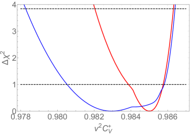
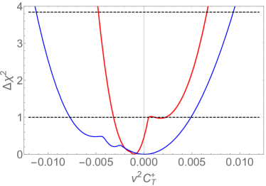
Figure 4: Marginalized $\Delta\chi^{2}\equiv\chi^{2}-\chi^{2}_{\rm min}$ distributions for the Wilson coefficients $C_{V}^{+}$ (left) and $C_{T}^{+}$ (right), with (red) and without (blue) taking account the input from mirror beta decay.

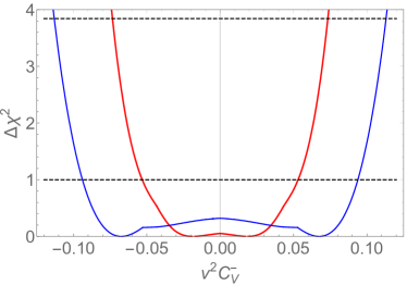
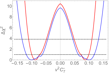
Figure 5: Marginalized $\Delta\chi^{2}\equiv\chi^{2}-\chi^{2}_{\rm min}$ distributions for the Wilson coefficients $C_{V}^{-}$ (left) and $C_{T}^{-}$ (right), with (red) and without (blue) taking account the input from mirror beta decay.

We close this section with a historical comment. One of the central questions in the 1950’s was whether the weak interactions were mediated by vector-axial or scalar-tensor currents. After some initial confusion, experiments settled on the former possibility, paving the way to the discovery of the SM. In fact, that conclusion has always hinged on simplifying assumptions that only a couple of Wilson coefficients of the Lee-Yang Lagrangian were present at the same time. The present analysis is the first complete and model-independent demonstration that the weak interactions involving the lightest quarks are of the vector-axial type. In contrast to the global fits performed in Refs. Boothroyd et al. (1984); Severijns et al. (2006) the present work includes also the extraction of the overall strength, keeping track of all correlations in a consistent way. At this point in history, such an observation has only an anecdotal value. Of more practical interest is that the present analysis provides the most up-to-date precise quantitative limits on possible departures from the vector-axial picture. We find that scalar and tensor currents associated with the left-hand neutrino have to be below a percent level at 95% CL. On the other hand, corrections from scalar and tensor currents associated with the right-hand neutrino can be larger, ${\mathcal{O}}(10)$%.

5 Conclusions and Future Directions

In this paper we have discussed the constraints from nuclear beta decays on the parameters of the effective Lee-Yang Lagrangian describing the weak interactions between nucleons, electrons, and neutrinos, paying special attention to the role played by mirror decays. The Wilson coefficients of this Lagrangian carry precious information about physics occurring at higher-energies compared to the nuclear scale. First, they are sensitive to the fundamental SM parameters, specifically to the combination $V_{ud}/v^{2}=\sqrt{2}G_{F}V_{ud}$. Second, they are affected by non-perturbative QCD entering via the nucleon charges $g_{V,A,S,T}$, and also by loop corrections which in part have to be evaluated in the non-perturbative regime as well. Finally, the Wilson coefficient are sensitive to physics beyond the SM, that is to masses and interaction strength of new hypothetical particles ($Z^{\prime}$ bosons, leptoquarks, etc.) with masses in the 1 GeV - 100 TeV range. We constructed a global likelihood function, using the latest experimental and theoretical input for a broad selection of allowed beta transitions. This allows us to extract the most up-to-date constraints on the Wilson coefficients in the Lee-Yang Lagrangian in (3).

Two hallmarks stand out in the present analysis as compared to previous works. One is that we perform a completely general model-independent fit, allowing all the leading order Wilson coefficients in the Lee-Yang Lagrangian to be simultaneously present. This follows the lines of analyses in Refs. Boothroyd et al. (1984); Severijns et al. (2006) but allowing in addition the extraction of the overall interaction strength in a consistent fashion. Therefore, the results obtained in this work can be applied to constrain generic new physics models that, at low energies, lead to an arbitrary pattern of vector, axial, scalar, and tensor currents. Moreover, the present results are valid for models with only left-handed neutrinos (as in the SM), as well as for models with both left- and right-handed neutrinos in the low-energy spectrum. The other hallmark is that we take into account measurements of half-lives and correlations in mirror beta transitions. Previously, mirror transitions have been employed to extract a value of the $V_{ud}$ matrix element in the SM scenario Naviliat-Cuncic and Severijns (2009). However, it is the first time that they are used in a consistent and global way to constrain new physics beyond the SM. In our analysis we include the data on beta decays of ¹⁷F, ¹⁹Ne, ²¹Na, ²⁹P, ³⁵Ar, and ³⁷K. The distinguishing feature of these nuclei is that not only their half-life but also some correlation parameter ($a$, $A$, or $B$) has been measured with a decent accuracy. This allows one, simultaneously, to determine the mixing parameters $\rho$ for these transition and to constrain several new combinations of the Lee-Yang Wilson coefficients.

It is also worth stressing that the present analysis incorporates for the first time some recent developments in non-mirror decays. They encompass theoretical aspects, such as the inclusion of the nuclear-structure dependent corrections pointed out in Refs. Seng et al. (2018); Gorchtein (2019), and experimental developments, such as the PERKEO-III measurement of the neutron beta asymmetry Markisch et al. (2019).

The results for the confidence intervals are given in Eqs. (19), (23), and (26), depending on the assumptions about the pattern of Wilson coefficients present in the Lagrangian. For the SM scenario and the BSM scenario involving only left-handed neutrinos, the present results supersede therefore those of Ref. Gonzalez-Alonso et al. (2019). Eq. (19) assumes the SM as the underlying theory and thus the only Wilson coefficients present are $C_{V}^{+}$ and $C_{A}^{+}$, as a consequence of the $V$-$A$ structure of the weak interactions. Eq. (23) assumes that the particle spectrum at low energies of order  2 GeV is that predicted by the SM, in particular that right-handed neutrinos are absent. However, it allows for generic new physics contributions, which manifest as scalar and tensor currents parameterized by the Wilson coefficients $C_{S}^{+}$ and $C_{T}^{+}$. Finally, Eq. (26) is the most general scenario, as it allows for the presence of right-handed neutrinos in the low-energy spectrum. Here, the relevant weak interactions are described by 8 Wilson coefficients: $C_{V,A,S,T}^{+}$ characterizing the vector, axial, scalar, and tensor currents with a left-handed neutrino, and $C_{V,A,S,T}^{-}$ characterizing the same currents but with a right-handed neutrino. In all these 3 scenarios we obtain a stable fit and stringent constraints on the Wilson coefficients. At the quantitative level, our most important findings are:

• The relative uncertainty on $C_{V}^{+}$ and $C_{A}^{+}$ is ${\mathcal{O}}(10^{-4})$ in the SM scenario. Via Eq. (2.1) it translates to an ${\mathcal{O}}(10^{-4})$ precision measurement of $V_{ud}$ and $g_{A}$. The uncertainty on these parameters relaxes to ${\mathcal{O}}(10^{-3})$ in the general new physics scenario;

• In the scenario with left-handed neutrinos the uncertainty on $C_{S}^{+}$ and $C_{T}^{+}$ is ${\mathcal{O}}(10^{-3})$ in the units of $1/v^{2}$, where $v\approx 246$ GeV. This implies that nuclear observables are sensitive to new particles with ${\mathcal{O}}(10)$ TeV masses and order one couplings to the SM, or with ${\mathcal{O}}(100)$ TeV masses and maximally strong coupling to the SM. In the presence of right-handed neutrinos these bounds are relaxed only by an ${\mathcal{O}}(2)$ factor;

• The uncertainty on the Wilson coefficients $C_{X}^{-}$ characterizing weak interactions of the right-handed neutrino is much larger, ${\mathcal{O}}(10^{-1})$ in the units of $1/v^{2}$. That is because the contributions from right-handed neutrinos to the nuclear observables enter only at the quadratic level in $C_{X}^{-}$.

• In the scenario with only left-handed neutrinos, the current data do not show any hint of new physics effects, that is to stay, $C_{S}^{+}$ and $C_{T}^{+}$ are compatible with zero within $1\sigma$ confidence level. On the other hand, in the general scenario the data show a $3.2\sigma$ indication for new physics manifesting via right-handed tensor currents with $|C_{T}^{-}|\sim 0.1/v^{2}$. That Wilson coefficient could be generated e.g. via a leptoquark with the mass in the TeV range and ${\mathcal{O}}(1)$ couplings to the light quarks, electron and right-handed neutrino. It is not clear, however, whether a phenomenologically viable model of this kind can be constructed, given the constraints from direct and Drell-Yan searches at the LHC Cirigliano et al. (2013b).

The inclusion of mirror transitions in the global fit has little effect in the SM scenario and in the BSM scenario with only left-handed neutrinos, where the precise data from the superallowed and neutron decays dominate the final constraints. On the other hand, the mirror transitions are vital to lift approximate degeneracies in the parameter space of the more general scenario with right-handed neutrinos. Here, the confidence intervals for the Wilson coefficients shrink by a factor of two due to the inclusion of the mirror data. Incidentally, the hint for a non-zero $C_{T}^{-}$ is slightly enhanced (by one unit of $\chi^{2}$) after including the mirror data. All this demonstrates the potential importance of mirror transitions as a means to search for new physics.

Measurement	17F	19Ne	21Na	29P	35Ar	37K
$\Delta a=10^{-3}$	1.3	1.2	1.6	1.4	1.6	1.3
$\Delta\tilde{A}=10^{-3}$	1.0	1.2	1.4	1.4	1.7	1.1
$\Delta\tilde{A}=10^{-3}$, ${\Delta{\cal F}t/{\cal F}t}=5\times 10^{-4}$	1.0	1.2	1.5	2.1	3.2	1.2
$\Delta\tilde{A}=10^{-4}$	1.4	3.1	2.1	1.5	1.8	1.4
$\Delta\tilde{A}=10^{-4}$, ${\Delta{\cal F}t/{\cal F}t}=5\times 10^{-4}$	1.5	3.8	3.8	3.8	3.9	3.4

Table 7: Potential improvements of the determination of the CKM matrix element $V_{ud}$ in the SM using only mirror decays with respect to the current extraction, $V_{ud}^{mirror}=0.97424(95)$. A given row and column indicate the observable and transition, respectively, that is added to the current dataset. We remind the reader that an improvement of a 3.4 (1.8) factor is required to reach the current $V_{ud}$ extractions from superallowed (neutron) data.

We close with a comment about the prospects for improving the constraints presented in this work. As shown in Table 1, past measurements of correlations in mirror decays are typically at the $10^{-2}$ level, with the notable exception of $\tilde{A}(^{37}{\rm K})$ which has a $3\times 10^{-3}$ uncertainty. On the other hand, ${\cal F}t$ values in mirror decays are much better known, with typical uncertainties in the $(0.5-1.8)\times 10^{-3}$ range. The expected sensitivity of improved beta decay experiments, many of which involve mirror nuclei, was recently discussed in Ref. Cirigliano et al. (2019). Our goal here is merely to establish a number of goalposts, to serve as a simple reference for planning future experiments. Potential improvements of the $V_{ud}$ determination from mirror decays are shown in Table 7 for the SM scenario. We see for instance that a new per-mille-accuracy $A$ measurement in ³⁵Ar will shrink the error bars by a 1.7 factor, producing a $V_{ud}^{mirror}$ extraction as precise as the current one from neutron decay. A more significant improvement would require knowledge of some correlation and the corresponding ${\cal F}t$ value with an ${\mathcal{O}}(10^{-4})$ accuracy. Beyond the SM, the impact on mirror-only fits will be far more consequential. As one can see in Table 5, the existing mirror data provide loose constraints on the SM and new physics parameters in the BSM scenario with only left-handed neutrinos. Any new per-mille-level correlation measurement will help lifting approximately flat directions in the parameter space, leading to a significant strengthening of the mirror-only constraints. On the other hand, it is less trivial for the new mirror measurements to make an impact in the global fit, where they have to compete with very precise superallowed and neutron data. We would need an ${\mathcal{O}}(10^{-4})$-level correlation measurement for a lighter mirror nuclei (¹⁷F or ¹⁹Ne) to have a non-negligible improvement in the BSM bounds. Finally, in the general BSM scenario with right-handed neutrinos the future mirror data will continue playing an outstanding role, whether in the mirror-only or in the global fit. In this case, because of the many-dimensional parameter space and the existence of multiple quasi-degenerate minima, any new per-mille level mirror measurement will be invaluable for reducing the error bars on both the SM and new physics parameters.

Appendix A Gamow-Teller decays

For completeness, in this appendix we summarize the theoretical expressions for the correlation parameters in Gamow-Teller (GT) beta decays used in the global fit. We define

$$\hat{\xi}_{\rm GT}\equiv(C_{A}^{+})^{2}+(C_{T}^{+})^{2}+(C_{A}^{-})^{2}+(C_{T}^{-})^{2}.$$ (27)

The $\beta$-$\nu$ correlation is then expressed by the Wilson coefficient of the Lee-Yang Lagrangian in Eq. (3) as

$$\hat{\xi}_{\rm GT}a_{\rm GT}=-{1\over 3}\bigg{[}(C_{A}^{+})^{2}-(C_{T}^{+})^{2}+(C_{A}^{-})^{2}-(C_{T}^{-})^{2}\bigg{]}.$$ (28)

The expression for the $\beta$-asymmetry depends on relative spins of the initial (J) and final (J’) state nuclei. For $J^{\prime}=J-1$ we have

$$\hat{\xi}_{\rm GT}A_{\rm GT}=\mp\bigg{\{}(C_{A}^{+})^{2}-(C_{T}^{+})^{2}-(C_{A}^{-})^{2}+(C_{T}^{-})^{2}\bigg{\}},$$ (29)

while for $J^{\prime}=J+1$ we have

$$\hat{\xi}_{\rm GT}A_{\rm GT}=\pm{J\over J+1}\bigg{\{}(C_{A}^{+})^{2}-(C_{T}^{+})^{2}-(C_{A}^{-})^{2}+(C_{T}^{-})^{2}\bigg{\}}.$$ (30)

Finally, the ratio of beta polarizations in pure Fermi and GT transitions is given by the expression:

$${P_{\rm F}\over P_{\rm GT}} = {(C_{V}^{+})^{2}-(C_{S}^{+})^{2}-(C_{V}^{-})^{2}+(C_{S}^{-})^{2}\over(C_{V}^{+})^{2}+(C_{S}^{+})^{2}+(C_{V}^{-})^{2}+(C_{S}^{-})^{2}-2\langle m_{e}/E_{e}\rangle_{F}\big{[}C_{V}^{+}C_{S}^{+}+C_{V}^{-}C_{S}^{-}\big{]}}$$ (31)

$$\times {(C_{A}^{+})^{2}+(C_{T}^{+})^{2}+(C_{A}^{-})^{2}+(C_{T}^{-})^{2}-2\langle m_{e}/E_{e}\rangle_{GT}\big{[}C_{A}^{+}C_{T}^{+}+C_{A}^{-}C_{T}^{-}\big{]}\over(C_{A}^{+})^{2}-(C_{T}^{+})^{2}-(C_{A}^{-})^{2}+(C_{T}^{-})^{2}}.$$

Appendix B Data for non-mirror beta decays

In this section we collect the additional experimental values for observables used in the analysis. The values for mirror beta decays are listed in Table 1.

Table 8: Data from superallowed decays used in the fits Hardy and Towner (2020).

Parent	${\cal F}t$ [s]	$\langle m_{e}/E_{e}\rangle$
10C	$3075.7\pm 4.4$	0.619
14O	$3070.2\pm 1.9$	0.438
22Mg	$3076.2\pm 7.0$	0.308
26mAl	$3072.4\pm 1.1$	0.300
26Si	$3075.4\pm 5.7$	0.264
34Cl	$3071.6\pm 1.8$	0.234
34Ar	$3075.1\pm 3.1$	0.212
38mK	$3072.9\pm 2.0$	0.213
38Ca	$3077.8\pm 6.2$	0.195
42Sc	$3071.7\pm 2.0$	0.201
46V	$3074.3\pm 2.0$	0.183
50Mn	$3071.1\pm 1.6$	0.169
54Co	$3070.4\pm 2.5$	0.157
62Ga	$3072.4\pm 6.7$	0.142
74Rb	$3077\pm 11$	0.125

Table 8 lists the ${\cal F}t$ values for the superallowed decays used in the fits. These are all $\beta^{+}$ transitions of the Fermi type between nuclei of spin 0 and positive parity. The ${\cal F}t$ values are copied from Table XVI of Ref. Hardy and Towner (2020). The central values take into account both the $\delta_{R}^{\prime}$ correction and the effects pointed out in Refs. Seng et al. (2018); Gorchtein (2019), however the errors do not include the associated theoretical uncertainties as they are strongly correlated between the decays. The fits carried out in the present work do take into account those correlated errors following Eq. (18). The $\langle m_{e}/E_{e}\rangle$ values are calculated using Eq. (7).

Table 9: Inputs from neutron decay used in the fits.

Observable	Value	S factor	$\langle m_{e}/E_{e}\rangle$	References
$\tau_{n}$ (s)	879.75(76)	1.9	0.655	Mampe et al. (1993); Byrne and Dawber (1996); Serebrov et al. (2005); Pichlmaier et al. (2010); Steyerl et al. (2012); Yue et al. (2013); Ezhov et al. (2018); Arzumanov et al. (2015); Pattie et al. (2018); Serebrov et al. (2018)
$\tilde{A}_{n}$	$-0.11958(21)$	1.2	0.569	Bopp et al. (1986); Liaud et al. (1997); Yerozolimsky et al. (1997); Mund et al. (2013); Brown et al. (2018); Markisch et al. (2019); Zyla et al. (2020)
$\tilde{B}_{n}$	0.9805(30)		0.591	Kuznetsov et al. (1995); Serebrov et al. (1998); Kreuz et al. (2005); Schumann et al. (2007)
$\lambda_{AB}$	$-1.2686(47)$		0.581	Mostovoi et al. (2001)
$a_{n}$	$-0.10426(82)$			Stratowa et al. (1978); Byrne et al. (2002); Beck et al. (2020)
$\tilde{a}_{n}$	$-0.1090(41)$		0.695	Darius et al. (2017)

The input from neutron decay used in the fits is shown in Table 9. When multiple references are given, the value is a Gaussian average of several experimental results. For the neutron lifetime, due to mutually inconsistent measurements, the error is inflated by the scale factor $S=1.9$ following the standard PDG procedure Zyla et al. (2020). Contrary to the latest PDG edition Zyla et al. (2020), we do not discard the beam measurements Byrne and Dawber (1996); Yue et al. (2013) following the arguments of Ref. Czarnecki et al. (2018), since these arguments are valid only in the SM context. In fact, as shown in Fig. 6, allowing for scalar and tensor currents in the effective Lagrangian, the global fit actually predicts a central value of $\tau_{n}$ closer to the beam than to the bottle results Mampe et al. (1993); Serebrov et al. (2005); Pichlmaier et al. (2010); Steyerl et al. (2012); Ezhov et al. (2018); Arzumanov et al. (2015); Pattie et al. (2018); Serebrov et al. (2018), although compatible with both of them.

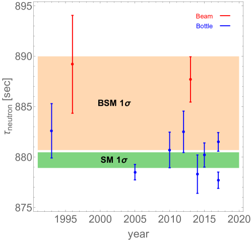
Figure 6: Neutron lifetime prediction in a global fit that includes all other measurements listed in Appendix B. Bottle measurements are favored in the SM fit (green band) but not in the BSM scenario with only left-handed neutrinos (salmon band) (cf. Section 4.2).

In the combination of the $\beta$-asymmetry measurements $\tilde{A}_{n}$ we inflate the error by the scale factor $S=1.2$, again following PDG Zyla et al. (2020). For the $\tau_{n}$ measurement, $\langle m_{e}/E_{e}\rangle$ is calculated using Eq. (7); for the remaining measurements we use the effective $\langle m_{e}/E_{e}\rangle$ values provided in Ref. Gonzalez-Alonso et al. (2019), which take into account the experimental conditions.

Table 10: Data from correlation measurements in pure Fermi and pure Gamow-Teller decays used in the fits.

Parent	$J_{i}$	$J_{f}$	Type	Observable	Value	$\langle m_{e}/E_{e}\rangle$	Ref.
6He	0	1	GT/$\beta^{-}$	$\tilde{a}$	$-0.3308(30)$	0.286	Johnson et al. (1963)
32Ar	0	0	F/$\beta^{+}$	$\tilde{a}$	0.9989(65)	0.210	Adelberger et al. (1999)
38mK	0	0	F/$\beta^{+}$	$\tilde{a}$	0.9981(48)	0.161	Gorelov et al. (2005)
60Co	5	4	GT/$\beta^{-}$	$\tilde{A}$	$-1.014(20)$	0.704	Wauters et al. (2010)
67Cu	3/2	5/2	GT/$\beta^{-}$	$\tilde{A}$	0.587(14)	0.395	Soti et al. (2014)
114In	1	0	GT/$\beta^{-}$	$\tilde{A}$	$-0.994(14)$	0.209	Wauters et al. (2009)
14O/10C			F-GT/$\beta^{+}$	$P_{F}/P_{GT}$	0.9996(37)	0.292	Carnoy et al. (1991)
26Al/30P			F-GT/$\beta^{+}$	$P_{F}/P_{GT}$	1.0030 (40)	0.216	Wichers et al. (1987)

Finally, the present analysis includes an input from various correlation measurements in pure Fermi and pure Gamow-Teller decays. These are collected in Table 10.

References

- Cirigliano et al. (2013a) V. Cirigliano, S. Gardner, and B. Holstein, Prog. Part. Nucl. Phys. 71, 93 (2013a), arXiv:1303.6953 [hep-ph] .
- Naviliat-Cuncic and González-Alonso (2013) O. Naviliat-Cuncic and M. González-Alonso, Annalen Phys. 525, 600 (2013), arXiv:1304.1759 [hep-ph] .
- Vos et al. (2015) K. K. Vos, H. W. Wilschut, and R. G. E. Timmermans, Rev. Mod. Phys. 87, 1483 (2015), arXiv:1509.04007 [hep-ph] .
- Gonzalez-Alonso et al. (2019) M. Gonzalez-Alonso, O. Naviliat-Cuncic, and N. Severijns, Prog. Part. Nucl. Phys. 104, 165 (2019), arXiv:1803.08732 [hep-ph] .
- Zyla et al. (2020) P. Zyla et al. (Particle Data Group), PTEP 2020, 083C01 (2020).
- Lee and Yang (1956) T. D. Lee and C.-N. Yang, Phys. Rev. 104, 254 (1956).
- Jackson et al. (1957a) J. D. Jackson, S. B. Treiman, and H. W. Wyld, Nucl. Phys. 4, 206 (1957a).
- Ebel and Feldman (1957) M. Ebel and G. Feldman, Nuclear Physics 4, 213 (1957).
- Pich (1998) A. Pich, in Les Houches Summer School in Theoretical Physics, Session 68: Probing the Standard Model of Particle Interactions (1998) pp. 949–1049, arXiv:hep-ph/9806303 .
- Paul (1970) H. Paul, Nucl. Phys. A 154, 160 (1970).
- Boothroyd et al. (1984) A. Boothroyd, J. Markey, and P. Vogel, Phys. Rev. C 29, 603 (1984).
- Severijns et al. (2006) N. Severijns, M. Beck, and O. Naviliat-Cuncic, Rev. Mod. Phys. 78, 991 (2006), arXiv:nucl-ex/0605029 .
- Severijns et al. (2008) N. Severijns, M. Tandecki, T. Phalet, and I. S. Towner, Phys. Rev. C78, 055501 (2008), arXiv:0807.2201 [nucl-ex] .
- Naviliat-Cuncic and Severijns (2009) O. Naviliat-Cuncic and N. Severijns, Phys. Rev. Lett. 102, 142302 (2009), arXiv:0809.0994 [nucl-ex] .
- Beck et al. (2020) M. Beck et al., Phys. Rev. C 101, 055506 (2020), arXiv:1908.04785 [nucl-ex] .
- Aghanim et al. (2020) N. Aghanim et al. (Planck), Astron. Astrophys. 641, A6 (2020), arXiv:1807.06209 [astro-ph.CO] .
- de Blas et al. (2018) J. de Blas, J. Criado, M. Perez-Victoria, and J. Santiago, JHEP 03, 109 (2018), arXiv:1711.10391 [hep-ph] .
- Herczeg (2001) P. Herczeg, Prog. Part. Nucl. Phys. 46, 413 (2001).
- Ademollo and Gatto (1964) M. Ademollo and R. Gatto, Phys. Rev. Lett. 13, 264 (1964).
- Aoki et al. (2020) S. Aoki et al. (Flavour Lattice Averaging Group), Eur. Phys. J. C 80, 113 (2020), arXiv:1902.08191 [hep-lat] .
- Chang et al. (2018) C. Chang et al., Nature 558, 91 (2018), arXiv:1805.12130 [hep-lat] .
- Gupta et al. (2018) R. Gupta, Y.-C. Jang, B. Yoon, H.-W. Lin, V. Cirigliano, and T. Bhattacharya, Phys. Rev. D98, 034503 (2018), arXiv:1806.09006 [hep-lat] .
- Gonzalez-Alonso and Martin Camalich (2014) M. Gonzalez-Alonso and J. Martin Camalich, Phys. Rev. Lett. 112, 042501 (2014), arXiv:1309.4434 [hep-ph] .
- Seng et al. (2018) C.-Y. Seng, M. Gorchtein, H. H. Patel, and M. J. Ramsey-Musolf, Phys. Rev. Lett. 121, 241804 (2018), arXiv:1807.10197 [hep-ph] .
- Czarnecki et al. (2019) A. Czarnecki, W. J. Marciano, and A. Sirlin, Phys. Rev. D 100, 073008 (2019), arXiv:1907.06737 [hep-ph] .
- Seng et al. (2020) C.-Y. Seng, X. Feng, M. Gorchtein, and L.-C. Jin, Phys. Rev. D 101, 111301 (2020), arXiv:2003.11264 [hep-ph] .
- Hayen (2021) L. Hayen, Phys. Rev. D 103, 113001 (2021), arXiv:2010.07262 [hep-ph] .
- Jackson et al. (1957b) J. D. Jackson, S. B. Treiman, and H. W. Wyld, Phys. Rev. 106, 517 (1957b).
- Holstein (1974) B. R. Holstein, Rev. Mod. Phys. 46, 789 (1974), [Erratum: Rev. Mod. Phys.48,673(1976)].
- Hayen et al. (2018) L. Hayen, N. Severijns, K. Bodek, D. Rozpedzik, and X. Mougeot, Rev. Mod. Phys. 90, 015008 (2018), arXiv:1709.07530 [nucl-th] .
- Hayen and Young (2020) L. Hayen and A. R. Young, (2020), arXiv:2009.11364 [nucl-th] .
- Hardy and Towner (2005) J. C. Hardy and I. S. Towner, Phys. Rev. C71, 055501 (2005), arXiv:nucl-th/0412056 .
- Hayen and Severijns (2019) L. Hayen and N. Severijns, (2019), arXiv:1906.09870 [nucl-th] .
- Czarnecki et al. (2018) A. Czarnecki, W. J. Marciano, and A. Sirlin, Phys. Rev. Lett. 120, 202002 (2018), arXiv:1802.01804 [hep-ph] .
- Towner and Hardy (2010) I. S. Towner and J. C. Hardy, Rept. Prog. Phys. 73, 046301 (2010).
- Wilkinson (1982) D. H. Wilkinson, Nucl. Phys. A377, 474 (1982).
- Gonzalez-Alonso and Naviliat-Cuncic (2016) M. Gonzalez-Alonso and O. Naviliat-Cuncic, Phys. Rev. C94, 035503 (2016), arXiv:1607.08347 [nucl-ex] .
- (38) IAEA-database, https://www-nds.iaea.org/nuclearmoments/.
- Fenker et al. (2018) B. Fenker et al., Phys. Rev. Lett. 120, 062502 (2018), arXiv:1706.00414 [nucl-ex] .
- Vetter et al. (2008) P. Vetter, J. Abo-Shaeer, S. Freedman, and R. Maruyama, Phys. Rev. C 77, 035502 (2008), arXiv:0805.1212 [nucl-ex] .
- (41) L. Hayen, Private communication.
- Melconian et al. (2007) D. Melconian et al., Phys. Lett. B 649, 370 (2007).
- Combs et al. (2020) D. Combs, G. Jones, W. Anderson, F. Calaprice, L. Hayen, and A. Young, (2020), arXiv:2009.13700 [nucl-ex] .
- Shidling et al. (2014) P. D. Shidling et al., Phys. Rev. C90, 032501 (2014), arXiv:1407.1742 [nucl-ex] .
- Rebeiro et al. (2019) B. Rebeiro et al., Phys. Rev. C 99, 065502 (2019), arXiv:1810.02331 [nucl-ex] .
- Karthein et al. (2019) J. Karthein et al., Phys. Rev. C 100, 015502 (2019), [Erratum: Phys.Rev.C 101, 049901 (2020)], arXiv:1906.01538 [nucl-ex] .
- Wang et al. (2017) M. Wang, G. Audi, F. G. Kondev, W. Huang, S. Naimi, and X. Xu, Chinese Physics C 41, 030003 (2017).
- Brodeur et al. (2016) M. Brodeur et al., Phys. Rev. C 93, 025503 (2016).
- Severijns et al. (1989) N. Severijns, J. Wouters, J. Vanhaverbeke, and L. Vanneste, Phys. Rev. Lett. 63, 1050 (1989).
- Calaprice et al. (1975) F. Calaprice, S. Freedman, W. Mead, and H. Vantine, Phys. Rev. Lett. 35, 1566 (1975).
- Long et al. (2020) J. Long et al., Phys. Rev. C 101, 015501 (2020).
- Masson and Quin (1990) G. Masson and P. Quin, Phys. Rev. C 42, 1110 (1990).
- Garnett et al. (1988) J. Garnett, E. Commins, K. Lesko, and E. Norman, Phys. Rev. Lett. 60, 499 (1988).
- Converse et al. (1993) A. Converse et al., Phys. Lett. B 304, 60 (1993).
- Markisch et al. (2019) B. Markisch et al., Phys. Rev. Lett. 122, 242501 (2019), arXiv:1812.04666 [nucl-ex] .
- Stratowa et al. (1978) C. Stratowa, R. Dobrozemsky, and P. Weinzierl, Phys. Rev. D 18, 3970 (1978).
- Byrne et al. (2002) J. Byrne, P. Dawber, M. D. van der Grinten, C. Habeck, F. Shaikh, J. Spain, R. Scott, C. Baker, K. Green, and O. Zimmer, J. Phys. G 28, 1325 (2002).
- Seng et al. (2019) C. Y. Seng, M. Gorchtein, and M. J. Ramsey-Musolf, Phys. Rev. D 100, 013001 (2019), arXiv:1812.03352 [nucl-th] .
- Gorchtein (2019) M. Gorchtein, Phys. Rev. Lett. 123, 042503 (2019), arXiv:1812.04229 [nucl-th] .
- Hardy and Towner (2020) J. Hardy and I. Towner, Phys. Rev. C 102, 045501 (2020).
- Towner and Hardy (2008) I. S. Towner and J. C. Hardy, Phys. Rev. C77, 025501 (2008), arXiv:0710.3181 [nucl-th] .
- Hardy and Towner (2015) J. C. Hardy and I. S. Towner, Phys. Rev. C91, 025501 (2015), arXiv:1411.5987 [nucl-ex] .
- Towner and Hardy (2002) I. Towner and J. Hardy, Phys. Rev. C 66, 035501 (2002), arXiv:nucl-th/0209014 .
- Towner (1994) I. Towner, Phys. Lett. B 333, 13 (1994), arXiv:nucl-th/9405031 .
- Towner (1992) I. Towner, Nucl. Phys. A 540, 478 (1992).
- Hardy and Towner (2018) J. Hardy and I. Towner, in 13th Conference on the Intersections of Particle and Nuclear Physics (2018) arXiv:1807.01146 [nucl-ex] .
- Feng et al. (2020) X. Feng, M. Gorchtein, L.-C. Jin, P.-X. Ma, and C.-Y. Seng, Phys. Rev. Lett. 124, 192002 (2020), arXiv:2003.09798 [hep-lat] .
- Pocanic et al. (2004) D. Pocanic et al., Phys. Rev. Lett. 93, 181803 (2004), arXiv:hep-ex/0312030 [hep-ex] .
- Marciano and Sirlin (2006) W. J. Marciano and A. Sirlin, Phys. Rev. Lett. 96, 032002 (2006), arXiv:hep-ph/0510099 [hep-ph] .
- Jenkins et al. (2018) E. E. Jenkins, A. V. Manohar, and P. Stoffer, JHEP 03, 016 (2018), arXiv:1709.04486 [hep-ph] .
- Dekens and Stoffer (2019) W. Dekens and P. Stoffer, JHEP 10, 197 (2019), arXiv:1908.05295 [hep-ph] .
- González-Alonso et al. (2017) M. González-Alonso, J. Martin Camalich, and K. Mimouni, Phys. Lett. B 772, 777 (2017), arXiv:1706.00410 [hep-ph] .
- Cirigliano et al. (2010) V. Cirigliano, J. Jenkins, and M. Gonzalez-Alonso, Nucl. Phys. B830, 95 (2010), arXiv:0908.1754 [hep-ph] .
- Gonzalez-Alonso and Martin Camalich (2016) M. Gonzalez-Alonso and J. Martin Camalich, JHEP 12, 052 (2016), arXiv:1605.07114 [hep-ph] .
- Bhattacharya et al. (2012) T. Bhattacharya, V. Cirigliano, S. D. Cohen, A. Filipuzzi, M. Gonzalez-Alonso, M. L. Graesser, R. Gupta, and H.-W. Lin, Phys. Rev. D85, 054512 (2012), arXiv:1110.6448 [hep-ph] .
- Walker-Loud et al. (2020) A. Walker-Loud et al., PoS CD2018, 020 (2020), arXiv:1912.08321 [hep-lat] .
- Cirigliano et al. (2013b) V. Cirigliano, M. Gonzalez-Alonso, and M. L. Graesser, JHEP 02, 046 (2013b), arXiv:1210.4553 [hep-ph] .
- Hassan et al. (2021) M. T. Hassan et al., Phys. Rev. C 103, 045502 (2021), arXiv:2012.14379 [nucl-ex] .
- Cirigliano et al. (2019) V. Cirigliano, A. Garcia, D. Gazit, O. Naviliat-Cuncic, G. Savard, and A. Young, (2019), arXiv:1907.02164 [nucl-ex] .
- Mampe et al. (1993) W. Mampe, L. Bondarenko, V. Morozov, Y. Panin, and A. Fomin, JETP Lett. 57, 82 (1993).
- Byrne and Dawber (1996) J. Byrne and P. Dawber, Europhys. Lett. 33, 187 (1996).
- Serebrov et al. (2005) A. Serebrov et al., Phys. Lett. B 605, 72 (2005), arXiv:nucl-ex/0408009 .
- Pichlmaier et al. (2010) A. Pichlmaier, V. Varlamov, K. Schreckenbach, and P. Geltenbort, Phys. Lett. B 693, 221 (2010).
- Steyerl et al. (2012) A. Steyerl, J. Pendlebury, C. Kaufman, S. Malik, and A. Desai, Phys. Rev. C 85, 065503 (2012).
- Yue et al. (2013) A. Yue, M. Dewey, D. Gilliam, G. Greene, A. Laptev, J. Nico, W. Snow, and F. Wietfeldt, Phys. Rev. Lett. 111, 222501 (2013), arXiv:1309.2623 [nucl-ex] .
- Ezhov et al. (2018) V. Ezhov et al., JETP Lett. 107, 671 (2018), arXiv:1412.7434 [nucl-ex] .
- Arzumanov et al. (2015) S. Arzumanov, L. Bondarenko, S. Chernyavsky, P. Geltenbort, V. Morozov, V. Nesvizhevsky, Y. Panin, and A. Strepetov, Phys. Lett. B 745, 79 (2015).
- Pattie et al. (2018) J. Pattie, R.W. et al., Science 360, 627 (2018), arXiv:1707.01817 [nucl-ex] .
- Serebrov et al. (2018) A. Serebrov et al., Phys. Rev. C 97, 055503 (2018), arXiv:1712.05663 [nucl-ex] .
- Bopp et al. (1986) P. Bopp, D. Dubbers, L. Hornig, E. Klemt, J. Last, H. Schutze, S. Freedman, and O. Scharpf, Phys. Rev. Lett. 56, 919 (1986), [Erratum: Phys.Rev.Lett. 57, 1192 (1986)].
- Liaud et al. (1997) P. Liaud, K. Schreckenbach, R. Kossakowski, H. Nastoll, A. Bussiere, J. Guillaud, and L. Beck, Nucl. Phys. A 612, 53 (1997).
- Yerozolimsky et al. (1997) B. Yerozolimsky, I. Kuznetsov, Y. Mostovoy, and I. Stepanenko, Phys. Lett. B 412, 240 (1997).
- Mund et al. (2013) D. Mund, B. Maerkisch, M. Deissenroth, J. Krempel, M. Schumann, H. Abele, A. Petoukhov, and T. Soldner, Phys. Rev. Lett. 110, 172502 (2013), arXiv:1204.0013 [hep-ex] .
- Brown et al. (2018) M.-P. Brown et al. (UCNA), Phys. Rev. C 97, 035505 (2018), arXiv:1712.00884 [nucl-ex] .
- Kuznetsov et al. (1995) I. Kuznetsov, A. Serebrov, I. Stepanenko, A. Aldushchenkov, M. Lasakov, A. Kokin, Y. Mostovoi, B. Erozolimsky, and M. Dewey, Phys. Rev. Lett. 75, 794 (1995).
- Serebrov et al. (1998) A. Serebrov et al., J. Exp. Theor. Phys. 86, 1074 (1998).
- Kreuz et al. (2005) M. Kreuz et al., Phys. Lett. B 619, 263 (2005).
- Schumann et al. (2007) M. Schumann, T. Soldner, M. Deissenroth, F. Gluck, J. Krempel, M. Kreuz, B. Markisch, D. Mund, A. Petoukhov, and H. Abele, Phys. Rev. Lett. 99, 191803 (2007), arXiv:0706.3788 [hep-ph] .
- Mostovoi et al. (2001) A. Mostovoi et al., Phys. Atom. Nucl. 64, 1955 (2001), [Yad. Fiz.64,2040(2001)].
- Darius et al. (2017) G. Darius et al., Phys. Rev. Lett. 119, 042502 (2017).
- Johnson et al. (1963) C. Johnson, F. Pleasonton, and T. Carlson, Phys. Rev. 132, 1149 (1963).
- Adelberger et al. (1999) E. Adelberger, C. Ortiz, A. Garcia, H. Swanson, M. Beck, O. Tengblad, M. Borge, I. Martel, and H. Bichsel (ISOLDE), Phys. Rev. Lett. 83, 1299 (1999), [Erratum: Phys.Rev.Lett. 83, 3101 (1999)], arXiv:nucl-ex/9903002 .
- Gorelov et al. (2005) A. Gorelov et al., Phys. Rev. Lett. 94, 142501 (2005), arXiv:nucl-ex/0412032 .
- Wauters et al. (2010) F. Wauters et al., Phys. Rev. C 82, 055502 (2010), arXiv:1005.5034 [nucl-ex] .
- Soti et al. (2014) G. Soti et al., Phys. Rev. C 90, 035502 (2014), arXiv:1409.1824 [nucl-ex] .
- Wauters et al. (2009) F. Wauters, I. Kraev, M. Tandecki, E. Traykov, S. Van Gorp, and N. Severijns, Phys. Rev. C 80, 062501 (2009), arXiv:0901.0081 [nucl-ex] .
- Carnoy et al. (1991) A. Carnoy, J. Deutsch, T. Girard, and R. Prieels, Phys. Rev. C 43, 2825 (1991).
- Wichers et al. (1987) V. Wichers, T. Hageman, J. Van Klinken, H. Wilschut, and D. Atkinson, Phys. Rev. Lett. 58, 1821 (1987).