Key Challenges in Personalised Meta-paths Generation .
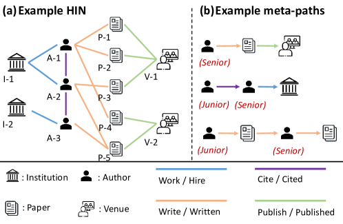
First, the definition of meta-paths requires rich domain knowledge that is extremely difficult to obtain in complex and semantic rich HINs DHWST20 G 𝐺 G N 𝑁 N R 𝑅 R T 𝑇 T ( N × R )^T . S u c h a h u g e s e t c a n r e s u l t i n a c o m b i n a t o r i a l e x p l o s i o n w h e n i n c r e a s i n g t h e s c a l e s o f N , R a n d T . S e c o n d , t h e r e p r e s e n t a t i o n c a p a c i t i e s o f m a n u a l l y − d e f i n e d m e t a − p a t h s a r e l i m i t e d t o a s p e c i f i c t a s k o n s p e c i f i c H I N s i n c e d i f f e r e n t G w i t h t h e s a m e N a n d R m a y h a v e d i f f e r e n t n o d e a t t r i b u t e s a n d r e l a t i o n t y p e s d i s t r i b u t i o n s . I t r e q u i r e s d e f i n i n g a p p r o p r i a t e m e t a − p a t h s f o r e a c h t a s k o n e a c h H I N , w h i c h i s e x t r e m e l y d i f f i c u l t f o r p r a c t i c a l a p p l i c a t i o n s . I n l i g h t o f t h e s e c h a l l e n g e s , w e p r o p o s e t o i n v e s t i g a t e H G R L w i t h t h e o b j e c t i v e s o f ( i ) l e a r n i n g t o g e n e r a t e a p e r s o n a l i s e d m e t a − p a t h f o r e a c h i n d i v i d u a l n o d e i n H I N s a u t o m a t i c a l l y , ( i i ) l e a r n i n g n o d e r e p r e s e n t a t i o n s e f f e c t i v e l y a n d e f f i c i e n t l y w i t h p e r s o n a l i s e d m e t a − p a t h s , a n d ( i i i ) r e t a i n i n g t h e e n d − t o − e n d t r a i n i n g s t r a t e g y t o a c h i e v e t a s k − o r i e n t e d o p t i m i s a t i o n . T o a c h i e v e t h e s e o b j e c t i v e s , w e p r e s e n t a n o v e l P e r s o n a l i s e d M e t a − p a t h b a s e d H e t e r o g e n e o u s G r a p h N e u r a l N e t w o r k ( P M − H G N N ) , t o u n l e a s h t h e p o w e r o f H G R L . 𝐊𝐞𝐲𝐈𝐝𝐞𝐚𝐬𝐨𝐟𝐏𝐌 − 𝐇𝐆𝐍𝐍 . G e n e r a l l y , w e a i m t o r e p l a c e t h e h u m a n e f f o r t s o n m e t a − p a t h g e n e r a t i o n w i t h a n R L a g e n t t o a d d r e s s t h e l i m i t a t i o n s o f t h e d e p e n d e n c y o n h a n d − c r a f t e d m e t a − p a t h s o f H G N N s . C o m p a r e d w i t h e x p e r t s w i t h d o m a i n k n o w l e d g e , t h e R L a g e n t c a n a d a p t i v e l y g e n e r a t e p e r s o n a l i s e d m e t a − p a t h s f o r e a c h i n d i v i d u a l n o d e i n t e r m s o f a s p e c i f i c t a s k / H I N t h r o u g h s e q u e n t i a l e x p l o r a t i o n a n d e x p l o i t a t i o n . T h a t s a i d , t h e o b t a i n e d m e t a − p a t h s a r e n o l o n g e r f o r s p e c i f i c t y p e s o f n o d e s b u t a r e p e r s o n a l i s e d f o r e a c h i n d i v i d u a l n o d e . B o t h g r a p h s t r u c t u r e a n d n o d e a t t r i b u t e s a r e c o n s i d e r e d i n t h e m e t a − p a t h g e n e r a t i o n p r o c e s s , a n d i t i s p r a c t i c a b l e f o r H I N s w i t h c o m p l e x s e m a n t i c s . A s i l l u s t r a t e d i n F i g . 2 , t h e m e t a − p a t h g e n e r a t i o n p r o c e s s c a n b e n a t u r a l l y c o n s i d e r e d a s a M a r k o v D e c i s i o n P r o c e s s ( M D P ) , i n w h i c h t h e n e x t r e l a t i o n t o e x t e n d i n g t h e m e t a − p a t h d e p e n d s o n t h e c u r r e n t s t a t e i n a m e t a − p a t h . M o r e o v e r , a n H G N N m o d e l i s p r o p o s e d t o l e a r n n o d e r e p r e s e n t a t i o n s f r o m t h e d e r i v e d m e t a − p a t h s t h a t c a n b e a p p l i e d t o a d o w n s t r e a m t a s k , s u c h a s n o d e c l a s s i f i c a t i o n . W e p r o p o s e t o e m p l o y a p o l i c y n e t w o r k ( a g e n t ) t o s o l v e t h i s M D P a n d u s e a n R L a l g o r i t h m e n h a n c e d b y a r e w a r d f u n c t i o n t o t r a i n t h e a g e n t . T h e r e w a r d f u n c t i o n i s d e f i n e d a s t h e p e r f o r m a n c e i m p r o v e m e n t o v e r h i s t o r i c a l p e r f o r m a n c e , w h i c h e n c o u r a g e s t h e R L a g e n t t o a c h i e v e b e t t e r a n d m o r e s t a b l e p e r f o r m a n c e . I n a d d i t i o n , w e f i n d t h a t t h e r e e x i s t s a l a r g e c o m p u t a t i o n a l r e d u n d a n c y d u r i n g t h e i n f o r m a t i o n a g g r e g a t i o n o n m e t a − p a t h s , t h u s w e d e v e l o p a n e f f i c i e n t s t r a t e g y t o a c h i e v e r e d u n d a n c y − f r e e a g g r e g a t i o n . W e s h o w c a s e a n i n s t a n c e o f o u r f r a m e w o r k , i . e . P M − H G N N , b y i m p l e m e n t i n g i t w i t h a c l a s s i c R L a l g o r i t h m , i . e . , D e e p Q − l e a r n i n g MKSRVBGRF15 . B e s i d e s , w e f u r t h e r p r o p o s e a n e x t e n s i o n o f P M − H G N N ++ t o d e a l w i t h t h e i s s u e s o f h i g h c o m p u t a t i o n a l c o s t a n d i g n o r i n g r e l a t i o n a l i n f o r m a t i o n i n P M − H G N N . S p e c i f i c a l l y , P M − H G N N g e n e r a t e s a m e t a − p a t h f o r e a c h n o d e a c c o r d i n g t o n o d e a t t r i b u t e s , w h i l e P M − H G N N ++ f u r t h e r e n a b l e s t h e m e t a − p a t h g e n e r a t i o n t o e x p l o r e t h e s t r u c t u r a l s e m a n t i c s o f H I N . P M − H G N N ++ i s a b l e t o n o t o n l y s i g n i f i c a n t l y a c c e l e r a t e t h e H G R L p r o c e s s b u t a l s o i m p r o v e t h e e f f e c t i v e n e s s o f l e a r n e d n o d e r e p r e s e n t a t i o n s w i t h p r o m i s i n g p e r f o r m a n c e o n d o w n s t r e a m t a s k s . 𝐌𝐚𝐢𝐧𝐂𝐨𝐧𝐭𝐫𝐢𝐛𝐮𝐭𝐢𝐨𝐧𝐬 . W e s u m m a r i s e o u r c o n t r i b u t i o n s b e l o w : •item 1st itemWe present a framework, PM-HGNN1footnote 11footnote 1Code and data are available at: https://github.com/zhiqiangzhongddu/PM-HGNN, to learn node representations in a HIN without hand-crafted meta-paths. An essential novelty of PM-HGNN is that the generated meta-paths are personalised to every individual node rather than general to each node type.•item 2nd itemWe propose an attention-based redundancy-free mechanism to reduce redundant computation during heterogeneous information aggregation on the derived meta-path instances.•item 3rd itemWe further develop an extension of PM-HGNN, PM-HGNN++, which not only improves the meta-path generation by incorporating node attributes and relational structure but also accelerates the training process.•item 4th itemExperiments conducted on node classification tasks with unsupervised and (semi-)supervised settings exhibit that our framework can significantly and consistently outperform 16 competing methods (up to %5.6 Micro-F1 improvements).
Advanced studies further reveal that PM-HGNN++ can identify meaningful meta-paths that human experts have ignored.
2 Related work
Relational Learning.
In the past decades, research focused on using frameworks that could represent a variable number of entities and the relationships that hold amongst them.
The interest in learning using this expressive representation formalism soon resulted in the emergence of a new subfield of machine learning that was described as relational learning V05 ; R08 BR98 SPC18 PCKD20 LSR20
Graph Neural Networks.
Existing GNNs generalise the convolutional operations of deep neural networks to deal with arbitrary graph-structured data.
Generally, a GNN model can be regarded as using the input graph structure to generate the computation graph of nodes for message passing, the local neighbourhood information is aggregated to get more effective contextual node representations in the network BZSL14 ; DBV16 ; KW17 ; VCCRLB18
Heterogeneous Graph Representation Learning.
HGRL aims to project nodes in a HIN into a low-dimensional vector space while preserving the heterogeneous node attributes and edges.
A recent survey presents a comprehensive overview of HGRL DHWST20 DCS17 ; FLL17 ; FHZYA18 MCMSZ15 ; SKBBTW18 ; ZSHSC19 ; WJSWYCY19 ; FZMK20 ; HDWS20 ; ZMGZ21 SKBBTW18 ZSHSC19 WJSWYCY19 VCCRLB18 FZMK20
A recent model, HGT HDWS20 YJKKK19 MCMSZ15 YLHZPH18 WDPH20 TSRMW18 ; AHMOP20
Discussion .
Table 8
3 Preliminaries
3.1 Problem Statement
Definition 1. (Heterogeneous Information Network ): A HIN is defined as a directed graph G = ( V , E , N , R ) ϕ : V → N φ : E → R N R v i x i ∈ R λ λ
Definition 2. (Meta-path ):
Given a HIN G Ω T ω 0 r 1 → ω 1 r 1 → … r T → ω T ω j ∈ N r i ∈ R
Definition 3. (Meta-path Instance ):
Given a meta-path Ω p Ω
Problem: Heterogeneous Graph Representation Learning.
We formulate heterogeneous graph representation learning (HGRL) as an information integration optimisation problem.
For a given HIN G f : ( V , E ) → R d ρ ρ { Ω j } ρ j = 1 v i ∈ V f G
3.2 Markov Decision Process
Markov Decision Process (MDP) is an idealised mathematical form to describe a sequential decision process that satisfies the Markov Property SB98 ( S , A , P , R ) S A P : S × A → ( 0 , 1 ) t P ( a t | s t ) s t ∈ S a t ∈ A R R : S × A → R a t s t
Figure 2 :
Illustration of generating meta-paths as an MDP.
Modelling HGRL with MDP .
As illustrated in Fig. 2 v A-1 s 1 v A-1 { Work , Cite , … } a 1 = argmax a ∈ A ( P ( a ∣ s 1 ) ) R ( s 1 , a 1 ) P 4
3.3 Solving MDP with Reinforcement Learning
Deep Reinforcement Learning (RL) is a family of algorithms that optimise the MDP with deep neural networks.
At each step t a t ∈ A s t ∈ S s t + 1 r t = R ( s t , a t ) P π : S → A E π [ ∑ t ′ = t T γ t ′ r t ′ ] T γ ∈ [ 0 , 1 ] γ ADBB17
Existing RL algorithms are mainly classified into two series: model-based and model-free algorithms.
Compared with model-based algorithms, model-free algorithms have better flexibility, as there is always the risk of suffering from model understanding errors, which in turn affects the learned policy ADBB17 MKSRVBGRF15 MKSRVBGRF15 Q ∗ Q ∗ ( s t , a t ) s t a t ∈ A a i R ( s t , a t ) + γ Q ∗ ( s t + 1 , a t + 1 ) Q Q ∗ MKSRVBGRF15
Q ( s t , a t ; θ ) = E s t + 1 [ R ( s t , a t ) + γ max a t + 1 ∈ A ( Q ( s t + 1 , a t + 1 ; θ ) ) ] , (1)
where θ ~ Q Q → ~ Q t → ∞
DQN exploits two techniques to stabilise the training:
(1) the memory buffer D separate target Q-network (^ Q
4 The PM-HGNN Framework
We present the overview of the proposed PM-HGNN in Fig. 3
Figure 3 :
Overview of PM-HGNN and PM-HGNN++ .
4.1 Personalised Meta-path Generation with RL
A personalised meta-path generation process with maximum T T
State (S : The state is a vector used to assist the decision policy to select a relation type to extend the personalised meta-paths for each node.
Hence, it is crucial to comprehensively encode existing parts of a meta-path into a state.
We adopt a gating mechanism to adaptively update the state.
Take v i Ω N v i s t Ω t
s t = q ∘ ( 1 | D ( v i ) | ∑ j ∈ D ( v i ) x j ) + ( 1 - q ) ∘ s t - 1 , (2)
where ∘ D ( v i ) t 1 | D ( v i ) | ∑ j ∈ D ( v i ) x j s t - 1 t - 1 q q = S i g m o i d ( f φ ( ( 1 | D ( v i ) | ∑ j ∈ D ( v i ) x j ) ∥ s t - 1 ) ) f φ VCCRLB18 1 - q
Action (A :
The action space is a set of relation types to be chosen by the policy network to extend the meta-path, and each relation type is labelled with a positive integer.
Note that we add a special action STOP to allow each node to have flexible-length meta-paths.
Beginning with the starting node v i STOP to finish the path generation process if encountering a state that includes any extra relationship to the current meta-path hurts the performance on the downstream task.
Decision Policy (P :
The decision policy aims at mapping a state in S A P ( a t | s t ; θ ) : S × A → ( 0 , 1 ) a ∈ A MKSRVBGRF15 H99 z 1 = W T 1 s t + b 1 z 2 = W T 2 z 1 + b 2 … ^ P = Softmax ( ϕ m ( W T m z m - 1 + b m ) )
W m
and
b m
denote the weight matrix and bias vector for the
m
-th layer’s perceptron, respectively.
The output ^ P ∈ ( 0 , 1 ) a t ∈ A
Reward Function (R :
We devise a reward function to encourage the RL agent to achieve better and more stable performance on downstream tasks.
We define the reward function R
R ( s t , a t ) = M ( s t , a t ) - ∑ j = t - b t - 1 M ( s j , a j ) b , (3)
where ∑ i = t - b t - 1 M ( s j , a j ) b t b M ( s t , a t ) H t [ v i ] M
Optimisation.
The proposed meta-path generation
at step t s t a t = arg max a ∈ A ( Q ( s t , a ; θ ) ) s t s t s t + 1 1 3
L Q ( θ ) = E T ∼ U ( D ) [ ( R ( s t , a t ) + γ max a t + 1 ∈ A ^ Q ( s t + 1 , a t + 1 ; θ - )
- Q ( s t , a t ; θ ) ) 2 ] , (4)
where T = ( s t , a t , s t + 1 , R ( s t , a t ) ) memory buffer D θ - separate target Q-network ^ Q max a t + 1 ∈ A ^ Q ( s t + 1 , a t + 1 ; θ - ) Q ( s t , a t ; θ )
4.2 Information Aggregation with Personalised Meta-paths
Due to the heterogeneity of nodes in HIN, various types of nodes have different attribute spaces.
Before the information aggregation, we first do a node type-specific transformation to project the latent features of different node types into the same space, given by: H 0 [ v i ] = W ω i ⋅ x i x i H 0 [ v i ] v i W ω i ω i = ϕ ( v i ) v i Ω
Figure 4 :
Comparison between information aggregation by conventional meta-path instances and the proposed redundancy-free computation.
(a) The sequential aggregation path instances generated from the meta-path
Ω PWritten _ by → Cite → Write → (A : Author , P : Paper ).
(b) The improved aggregation structure by our redundancy-free computation method with attention scores to distinguish messages from different nodes.
We first generate meta-path instances { p 1 , p 2 , … } Ω 4 Ω Ω : Paper Written _ by → Author Cite → Author Write → Paper ZSHSC19 WJSWYCY19 P 3 → A 2 P 5 → A 2 { P 3 , P 5 } → A 2 redundancy-free aggregation.
Besides, we learn the attention scores A t t ( v i , v j ) v i v j
Let H 0 [ v i ] v i { p 1 , p 2 , … } Ω H [ v i ]
H l [ v i ] = Aggregate v j ∈ I ( v i ) ( Att ( v i , v j ) ⋅ H l - 1 [ v j ] ) , (5)
where I ( v i ) v i { p 1 , p 2 , … } l ∈ { 1 , 2 , … , t } Aggregate ( ⋅ ) = R e l u ( Mean ( ⋅ ) ) Att ( ⋅ )
Att ( i , j ) = Softmax j ∈ I ( v i ) ( L e a k y R e l u ( W H l - 1 [ v j ] ∥ W H l - 1 [ v i ] ) ) , (6)
where W ∥ 5.4
Algorithm 1
4.3 Model Training
Training of HGNN.
Finally, the updated node representation H t [ v i ] L L = - ∑ v ∈ V L ∑ c = 0 C - 1 y v [ c ] ⋅ log ( H t [ v ] [ c ] ) V L C y v v H t [ v ] v M eval 1
4.4 PM-HGNN++
As seen in previous sections, PM-HGNN adopts the RL agent to generate meta-paths for HGRL adaptively.
However, reviewing the overall workflow of PM-HGNN, we identify two limitations.
(1) PM-HGNN neglects the relational structures of HIN while generating meta-paths;
(2) HGNN requires a large number of epochs to train their parameters and obtain node representations, which restricts the efficiency of PM-HGNN.
To be more specific, PM-HGNN generates meta-paths by only considering the node attribute information from the HIN, i.e., state s t 2 KW17 B T × B T T = ( s t , a t , s t + 1 , R ( s t , a t ) ) 2
New State (S .
To address the identified limitations, we propose an extension of PM-HGNN, PM-HGNN++ , which can utilise the structure information of HIN and significantly accelerate the meta-path generation process.
Our solution is to define a novel state instead of Eq. 2 H t - 1 [ v i ] v i S
s t = Normalise ( H t - 1 [ i ] ) , (7)
where Normalise B H [ v i ] - H m e a n H s t d H m e a n H s t d B normaliser is a common trick used in deep RL for stabilising the training when the S HLWXC17 H t [ i ] s t 7 ++ with the ability to handle graphs with diverse node attributes.
Algorithm 2 ++
New Training Process .
The training process can be further improved based on the new definition of the state.
The learned node representation can be further used to optimise HGNN’s parameters and update the RL agent.
We achieve such a kind of mutual optimisation between the RL agent and HGNN since the meta-paths are generated based on the current status of HGNN.
With this novel training process, we only need T T × B ++ in Algorithm 2 ++ in Sec. 5.4 ++ framework can adaptively generate a meta-path for the new node to compute its representation, which maintains the ability of HGNN to learn representations for newly added nodes.
4.5 Model Analysis
The proposed models can deal with various types of nodes and relations and fuse rich semantics in HINs.
Benefiting from the RL agent, personalised meta-paths are generated for different nodes, and the HGNN encoder allows information to transfer between nodes via diverse relations.
The RL agent that we adopted in this paper, i.e., Deep Q-learning (DQN), is hard to give the precise computation complexity FWXY20 5.4 8 Ω d O ( V Ω d 2 + E Ω d ) V Ω Ω E Ω O ( V Ω d 2 ) O ( E Ω d ) A t t ( ⋅ ) T 5.4 6
5 Experiments
5.1 Experimental Settings
Datasets.
We adopt three HIN datasets (IMDb and DBLP, ACM) WJSWYCY19 ; FZMK20 4 9 A
Competing Methods and Model Configuration.
We compare their performance against various state-of-the-art models.
They include 5 homogeneous graph representation learning models: LINE TQWZYM15 PAS14 KW17 VCCRLB18 SQLKHP16 DCS17 HYC18 SHZY19 ZWSLY20 SKBBTW18 WJSWYCY19 YJKKK19 FZMK20 HDWS20 LSR20 MCMSZ15 YLHZPH18 WDPH20 2 C E
Evaluation Settings.
We evaluate our models under node classification.
For the semi-supervised setting, we adopt the same settings as in MAGNN FZMK20 support vector machine (SVM) classifier to get the prediction results.
For the supervised setting, we use the same percentage of nodes for training and validation, respectively. Use the rest of the nodes for testing.
We report the average Micro-F1 and Macro-F1 scores of 10 runs with different seeds.
5.2 Experimental Results
Table 1 :
Experiment results (%) on the IMDb, DBLP and ACM datasets for the node classification task with unsupervised and semi-supervised settings.
MP2V stands for metapath2vec.
Best performance is marked in bold .
Semi-supervised Node Classification .
We present the results in Table 1 ++ performs consistently better than all competing methods across different proportions and datasets.
On IMDb, the performance gain obtained by PM-HGNN++ over the best competing method (MAGNN) is around (3.7 % - 5.08 % ++ apparently outperforms the strongest competing method (i.e., MAGNN) up to 2.4 % ++ .
In addition, among unsupervised competing methods, NSHE obtains better performance than other unsupervised methods, showing that network schema in HIN is helpful to obtain better representations.
Table 2 :
Experiment results (%) on the IMDb, DBLP and ACM datasets for the node classification task with supervised settings.
Best performance is marked in bold .
Supervised Node Classification .
We present the results in Table 2 ++ consistently outperforms all competing models on IMDb, DBLP and ACM datasets, with up to 5.6 % Micro-F1 .
Heterogeneous GNNs outperform homogeneous GNNs, and our PM-HGNN++ achieves the best performance.
This demonstrates the usefulness of heterogeneous relations and the advantages of generating appropriate personalised meta-paths for each node according to its attributes and relational structure.
5.3 Meta-path Analysis
Meta-path Generation Process Visualisation.
We visualise how the RL agent in PM-HGNN++ generates personalised meta-paths for each target node in Fig. 10 11 12 10 M 64.8 % → A 8.8 % → M T = 2 64.8 % 64.8 % Movie nodes select MA relation at step-1, and 8.8 % Movie nodes who selected MA at step-1, there are 8.8 % AM to extend the meta-path.
It is interesting to see that the RL agent selects the relation MA at the first step more often than the other one MD .
It means that a movie’s characteristic is more related to its actors than its director.
Besides, when step T = 2 STOP actions.
This shows that two short meta-paths, i.e., Movie MA → Actor Movie MD → Director 6.7 % - 9.4 % 5.2 11 12 B
Table 3 : Meta-paths designed by PM-HGNN++ on IMDb.
Overall Meta-path Statistics.
We further present meta-paths generated for most of the target nodes in Table 3 10 6 7 3 Movie nodes.
Two short meta-paths Movie MA → Actor Movie MD → Director Movie nodes’ representations.
However, GTN can only select several meta-paths for every node type; our model can identify personalised meta-paths for each node.
More analyses on Table 6 7 B
Figure 5 :
The average meta-path length generated by PM-HGNN++ on different datasets.
MLP (pos)/ MLP (neg) are groups of nodes that MLP makes correct and wrong classifications, respectively.
Meta-path Comparison.
In order to understand how does PM-HGNN++ generate personalised meta-paths for different nodes, we hereby present another analysis to investigate the designed meta-path lengths for nodes that can be correctly classified according to raw node attributes.
Specifically, we devide nodes into two groups, pos and neg , according to whether applying multi-layer perceptron (MLP) with node attributes can produce correct classification under supervised settings.
That said, correctly-classified nodes and incorrectly-classified ones are grouped into pos and neg , respectively.
Then, we calculate the average lengths of PM-HGNN++ generated meta-paths for nodes belonging to two groups.
The results are reported in Fig. 5 ++ tends to explore deeper relational neighbouring structure to enhance node representation learning, i.e., discriminating nodes with different labels from one another, if node attributes themselves cannot provide sufficient information.
Moreover, in the DBLP dataset, which has more complicated heterogeneous semantic patterns (4 node types and 6 relation types), node group MLP (neg ) has relatively longer meta-paths because PM-HGNN++ can have more options to explore and generate personalised meta-paths.
5.4 Model Analysis on PM-HGNN++
Figure 6 : Micro-F1 and the number of aggregations of PM-HGNN++ on IMDb, with different max steps.
Maximum Step T
We study how the influence of maximum step T 6 T ≥ 2 T = 1 T T = 2 5.2 T > 2
Figure 7 :
The relative numbers of aggregations (# of without the redundancy-free aggregation divided by # of with the redundancy-free aggregation) under different maximum steps on IMDb (left) and DBLP (right).
Redundancy-free Aggregation.
We investigate the influence of the redundancy-free improvement according to the number of aggregations with/without the improvement.
Fig. 7 T T = 2 T = 4
Figure 8 :
Run time analysis of meta-path generation for PM-HGNN and PM-HGNN++ under different max steps based on IMDb (left) and DBLP (right) datasets. The x-axis is the number of maximum timestep in generating meta-paths, and the y-axis is the relative time (i.e., the run time of PM-HGNN++ divided by the run time of PM-HGNN). Besides, the numbers at tops of bars indicate the run time values in seconds.
Run Time Analysis of Meta-path Generation.
As described in Sec. 4.4 ++ can accelerate the meta-path generation process through the proposed novel training process.
Here we compare the run time of PM-HGNN and PM-HGNN++ for personalised meta-paths generation.
We report their actual run time in seconds, and calculate the run time of PM-HGNN++ relative to PM-HGNN (i.e., relative time). The results on IMDb and DBLP datasets are shown in Fig. 8 ++ is less than 5 % ++ .
6 Conclusions and future work
We have studied in this paper the HGRL problem and identified the limitation of existing HGRL methods, i.e., mainly due to their dependency on hand-crafted meta-paths.
In order to fully unleash the power of HGRL, we presented a novel framework PM-HGNN and proposed one extension model PM-HGNN++ .
Compared with existing HGRL models, the most significant advantages of our framework lie in avoiding manual efforts in defining meta-paths of HGRL and generating personalised meta-paths for each individual node.
The experimental results demonstrated that our framework generally outperforms the competing approaches and discovers useful meta-paths that have been ignored by human expertise.
In the future, we plan to extend our framework to other tasks on HINs, such as online recommendation and knowledge graph completion and understanding PM-HGNN’s generated meta-paths is another promising direction.
\bmhead
Acknowledgments
This work is supported by the Luxembourg National Research Fund through grant PRIDE15/10621687/SPsquared, and supported by Ministry of Science and Technology (MOST) of Taiwan under grants 110-2221-E-006-136-MY3, 110-2221-E-006-001, and 110-2634-F-002-051.
References
\bibcommenthead
(1)
Sun, Y.,
Han, J.:
Mining heterogeneous information networks: a structural analysis approach.
ACM SIGKDD Explorations Newsletter
(2012)
(2)
Van Otterlo, M.:
A survey of reinforcement learning in relational domains.
Centre for Telematics and Information Technology (CTIT) University of Twente,
Tech. Rep
(2005)
(3)
Zheng, J.,
Ma, Q.,
Gu, H.,
Zheng, Z.:
Multi-view denoising graph auto-encoders on heterogeneous information
networks for cold-start recommendation.
In: Proceedings of the 2021 ACM Conference on Knowledge Discovery and
Data Mining (KDD),
pp. 2338–2348
(2021)
(4)
Wan, G.,
Du, B.,
Pan, S.,
Haffari, G.:
Reinforcement learning based meta-path discovery in large-scale
heterogeneous information networks.
In: Proceedings of the 2020 AAAI Conference on Artificial Intelligence
(AAAI),
pp. 6094–6101
(2020)
(5)
Wang, X.,
Ji, H.,
Shi, C.,
Wang, B.,
Ye, Y.,
Cui, P.,
Yu, P.S.:
Heterogeneous graph attention network.
In: Proceedings of the 2019 International Conference on World Wide Web
(WWW),
pp. 2022–2032
(2019)
(6)
Fu, X.,
Zhang, J.,
Meng, Z.,
King, I.:
MAGNN: metapath aggregated graph neural network for heterogeneous
graph embedding.
In: Proceedings of the 2020 International Conference on World Wide Web
(WWW),
pp. 2331–2341
(2020)
(7)
Dong, Y.,
Hu, Z.,
Wang, K.,
Sun, Y.,
Tang, J.:
Heterogeneous network representation learning.
In: Proceedings of the 2020 International Joint Conferences on
Artifical Intelligence (IJCAI),
pp. 4861–4867
(2020)
(8)
Dong, Y.,
Chawla, N.V.,
Swami, A.:
metapath2vec: Scalable representation learning for heterogeneous
networks.
In: Proceedings of the 2017 ACM Conference on Knowledge Discovery and
Data Mining (KDD),
pp. 135–144
(2017)
(9)
Fu, T.,
Lee, W.,
Lei, Z.:
Hin2vec: Explore meta-paths in heterogeneous information networks for
representation learning.
In: Proceedings of the 2017 ACM International Conference on
Information and Knowledge Management (CIKM),
pp. 1797–1806
(2017)
(10)
Shi, C.,
Hu, B.,
Zhao, W.X.,
Yu, P.S.:
Heterogeneous information network embedding for recommendation.
IEEE Transactions on Knowledge and Data Engineering
(2019)
(11)
Mikolov, T.,
Sutskever, I.,
Chen, K.,
Corrado, G.S.,
Dean, J.:
Distributed representations of words and phrases and their
compositionally.
In: Proceedings of the 2013 Annual Conference on Neural Information
Processing Systems (NIPS),
pp. 3111–3119
(2013)
(12)
Le, Q.V.,
Mikolov, T.:
Distributed representations of sentences and documents.
In: Proceedings of the 2014 International Conference on Machine
Learning (ICML),
pp. 1188–1196
(2014)
(13)
Hussein, R.,
Yang, D.,
Cudré-Mauroux, P.:
Are meta-paths necessary?: Revisiting heterogeneous graph embeddings.
In: Proceedings of the 2018 ACM International Conference on
Information and Knowledge Management (CIKM),
pp. 437–446
(2018)
(14)
Jiang, J.,
Li, Z.,
Ju, C.J.-,
Wang, W.:
MARU: meta-context aware random walks for heterogeneous network
representation learning.
In: Proceedings of the 2020 ACM International Conference on
Information and Knowledge Management (CIKM),
pp. 575–584
(2020)
(15)
Zhao, J.,
Wang, X.,
Shi, C.,
Liu, Z.,
Ye, Y.:
Network schema preserving heterogeneous information network
embedding.
In: Proceedings of the 2020 International Joint Conferences on
Artifical Intelligence (IJCAI),
pp. 1366–1372
(2020)
(16)
Kipf, T.N.,
Welling, M.:
Semi-supervised classification with graph convolutional networks.
In: Proceedings of the 2017 International Conference on Learning
Representations (ICLR)
(2017)
(17)
Velickovic, P.,
Cucurull, G.,
Casanova, A.,
Romero, A.,
Lio, P.,
Bengio, Y.:
Graph attention networks.
In: Proceedings of the 2018 International Conference on Learning
Representations (ICLR)
(2018)
(18)
Schlichtkrull, M.S.,
Kipf, T.N.,
Bloem, P.,
van den Berg, R.,
Titov, I.,
Welling, M.:
Modeling relational data with graph convolutional networks.
In: European Semantic Web Conference (ESWC),
pp. 593–607
(2019)
(19)
Zhang, C.,
Song, D.,
Huang, C.,
Swami, A.,
Chawla, N.V.:
Heterogeneous graph neural network.
In: Proceedings of the 2019 ACM Conference on Knowledge Discovery and
Data Mining (KDD),
pp. 793–803
(2019)
(20)
Mnih, V.,
Kavukcuoglu, K.,
Silver, D.,
Rusu, A.A.,
Veness, J.,
Bellemare, M.G.,
Graves, A.,
Riedmiller, M.A.,
Fidjeland, A.,
Ostrovski, G.,
Petersen, S.,
Beattie, C.,
Sadik, A.,
Antonoglou, I.,
King, H.,
Kumaran, D.,
Wierstra, D.,
Legg, S.,
Hassabis, D.:
Human-level control through deep reinforcement learning.
Nature
518 ,
529–533
(2015)
(21)
Meng, C.,
Cheng, R.,
Maniu, S.,
Senellart, P.,
Zhang, W.:
Discovering meta-paths in large heterogeneous information networks.
In: Proceedings of the 2015 International Conference on World Wide Web
(WWW),
pp. 754–764
(2015)
(22)
Yang, C.,
Liu, M.,
He, F.,
Zhang, X.,
Peng, J.,
Han, J.:
Similarity modeling on heterogeneous networks via automatic path
discovery.
In: European Conference on Machine Learning and Knowledge Discovery in
Databases (ECMLPKDD),
pp. 37–54
(2018)
(23)
Raedt, L.D.:
Logical and Relational Learning.
Cognitive Technologies,
(2008)
(24)
Blockeel, H.,
Raedt, L.D.:
Top-down induction of first-order logical decision trees.
Artif. Intell.
101 (1-2),
285–297
(1998)
(25)
Serafino, F.,
Pio, G.,
Ceci, M.:
Ensemble learning for multi-type classification in heterogeneous
networks.
IEEE Transactions on Knowledge and Data Engineering
30 (12),
2326–2339
(2018)
(26)
Petkovic, M.,
Ceci, M.,
Kersting, K.,
Dzeroski, S.:
Estimating the importance of relational features by using gradient
boosting.
In: International Symposium on Foundations of Intelligent Systems
(ISMIS).
Lecture Notes in Computer Science,
vol. 12117,
pp. 362–371
(2020)
(27)
Lavrac, N.,
Skrlj, B.,
Robnik-Sikonja, M.:
Propositionalization and embeddings: two sides of the same coin.
Machine Learning
109 (7),
1465–1507
(2020)
(28)
Bruna, J.,
Zaremba, W.,
Szlam, A.,
LeCun, Y.:
Spectral networks and locally connected networks on graphs.
In: Proceedings of the 2014 International Conference on Learning
Representations (ICLR)
(2014)
(29)
Defferrard, M.,
Bresson, X.,
Vandergheynst, P.:
Convolutional neural networks on graphs with fast localized spectral
filtering.
In: Proceedings of the 2016 Annual Conference on Neural Information
Processing Systems (NIPS),
pp. 3837–3845
(2016)
(30)
Fan, Y.,
Hou, S.,
Zhang, Y.,
Ye, Y.,
Abdulhayoglu, M.:
Gotcha - sly malware!: Scorpion A metagraph2vec based malware
detection system.
In: Proceedings of the 2018 ACM Conference on Knowledge Discovery and
Data Mining (KDD),
pp. 253–262
(2018)
(31)
Hu, Z.,
Dong, Y.,
Wang, K.,
Sun, Y.:
Heterogeneous graph transformer.
In: Proceedings of the 2020 International Conference on World Wide Web
(WWW),
pp. 2704–2710
(2020)
(32)
Yun, S.,
Jeong, M.,
Kim, R.,
Kang, J.,
Kim, H.J.:
Graph transformer networks.
In: Proceedings of the 2019 Annual Conference on Neural Information
Processing Systems (NeurIPS),
pp. 11960–11970
(2019)
(33)
Tanon, T.P.,
Stepanova, D.,
Razniewski, S.,
Mirza, P.,
Weikum, G.:
Completeness-aware rule learning from knowledge graphs.
In: Proceedings of the 2018 International Joint Conferences on
Artifical Intelligence (IJCAI),
pp. 5339–5343
(2018)
(34)
Ahmadi, N.,
Huynh, V.,
Meduri, V.V.,
Ortona, S.,
Papotti, P.:
Mining expressive rules in knowledge graphs.
ACM Journal of Data and Information Quality
(2020)
(35)
Sutton, R.S.,
Barto, A.G.:
Reinforcement learning: An introduction.
IEEE Transactions on Neural Networks and Learning Systems
9 (5),
1054–1054
(1998)
(36)
Arulkumaran, K.,
Deisenroth, M.P.,
Brundage, M.,
Bharath, A.A.:
Deep reinforcement learning: A brief survey.
IEEE Signal Processing Magazine
(2017)
(37)
Haykin, S.:
Neural networks: A comprehensive foundation.
Knowledge Engineering Review
(1999)
(38)
Hou, Y.,
Liu, L.,
Wei, Q.,
Xu, X.,
Chen, C.:
A novel DDPG method with prioritized experience replay.
In: Proceedings of the 2017 International Conference on Systems Man
and Cybernetics (SMC),
pp. 316–321
(2017)
(39)
Fan, J.,
Wang, Z.,
Xie, Y.,
Yang, Z.:
A theoretical analysis of deep q-learning.
In: Proceedings of the 2020 Annual Conference on Learning for Dynamics
and Control (L4DC).
Proceedings of Machine Learning Research,
vol. 120,
pp. 486–489
(2020)
(40)
Tang, J.,
Qu, M.,
Wang, M.,
Zhang, M.,
Yan, J.,
Mei, Q.:
Line: Large-scale information network embedding.
In: Proceedings of the 2015 International Conference on World Wide Web
(WWW),
pp. 1067–1077
(2015)
(41)
Perozzi, B.,
Al-Rfou, R.,
Skiena, S.:
Deepwalk: Online learning of social representations.
In: Proceedings of the 2014 ACM Conference on Knowledge Discovery and
Data Mining (KDD),
pp. 701–710
(2014)
(42)
Shang, J.,
Qu, M.,
Liu, J.,
Kaplan, L.M.,
Han, J.,
Peng, J.:
Meta-path guided embedding for similarity search in large-scale heterogeneous
information networks.
CoRR
abs/1610.09769
(2016)
Appendix A Datasets
The statistics of datasets are summarised in Table 4
IMDb is an online dataset about movies and television programs, including information such as cast, production crew and plot summaries.
We extract a subset of IMDb that contains 4 , 278 2 , 081 5 , 257 Action , Comedy and Drama , according to their genre information.
The attribute of each movie corresponds to elements of a bag of words (i.e., their plot keywords, 1 , 232
DBLP is an online computer science bibliography.
We extract a subset of DBLP that contains 4 , 057 1 , 4328 7 , 723 Database , Data mining , Machine learning and Information retrial .
Each author can be described by a bag of words (i.e., their paper keywords, 334 in total).
ACM is an online academic publication dataset.
We extract papers published in KDD, SIGMOD, SIGCOMM, MobiCOMM and VLDB and divided the papers into three classes (Database , Wireless Communication , and Data Mining ).
Then, we construct a HIN that comprises 3 , 025 5 , 835
Table 4 : Statistics of the datasets.
Figure 9 :
Meta-relation schema of three datasets.
Appendix B More Meta-paths Analysis
Figure 10 :
Actions that the RL agent takes on IMDb: (a), (b) and (c) correspond to PM-HGNN++ with max step T = 1 , 2 , 3
Table 5 :
All possible meta-paths on different datasets.
IMDb: Movie (M), Director (D), Actor (A);
DBLP: Author (A), Paper (P), Term (T), Venue (V);
ACM: Paper (P), Author (A), Subject (S).
We have introduced three datasets that we used in the experimental sections in Section 5.1 A 5 4 STOP action at each step.
That said, PM-HGNN variants allow to design meta-paths with flexible lengths at each step.
Figure 11 :
Actions that the RL agent takes on DBLP: (a), (b) and (c) correspond to PM-HGNN++ with max step T = 1 , 2 , 3
Table 6 : Meta-paths generated by PM-HGNN++ on DBLP.
Figure 12 :
Actions that the RL agent takes on ACM: (a), (b) and (c) correspond to PM-HGNN++ with max step T = 1 , 2 , 3
Table 7 : Meta-paths generated by PM-HGNN++ on ACM.
We present more meta-path analysis here.
Figure 11 12 ++ generates personalised meta-paths for each target node on DBLP and ACM datasets with different max steps under the semi-supervised setting, respectively
The percentages marked in the figure represent the fraction of nodes choosing the corresponding relation to extend the meta-path at that step.
Table 6 7 YJKKK19 ++ for the target nodes of DBLP and ACM datasets, respectively.
The meta-path generation process is shown in Figure 11 12 S
Appendix C Competing Methods
We adopt 5 homogeneous graph representation learning models and 10 heterogeneous graph representation learning models and 1 state-of-the-art relational learning model as competing methods.
1.
LINE TQWZYM15
2.
DeepWalk PAS14
3.
ESim SQLKHP16
4.
metapath2vec DCS17
5.
JUST HYC18
6.
HERec SHZY19
7.
NSHE ZWSLY20
8.
MLP H99
9.
GCN KW17
10.
GAT VCCRLB18
11.
RGCN SKBBTW18
12.
HAN WJSWYCY19
13.
GTN YJKKK19
14.
PropStar LSR20
15.
MAGNN FZMK20
16.
HGT HDWS20
For LINE and DeepWalk, we utilise the integrated implementations from GraphEmbedding.
For metapath2vec, RGCN, HAN and HGT, we utilise the integrated implementations from Deep Graph Library.
For GCN and GAT, we use the implementation from PytorGeometric.
For other methods, we adopt the official implementation provided in their published papers: ESim, JUST, HERec, NSHE, GTN, PropStart and MAGNN.
Appendix D Model Comparison
Table 8 :
Model comparison from various aspects: Heterogeneous Information Network (HIN), Node-wise Task (NT), End-to-end Training (E2E), Without Manual-defined Meta-paths (WMM), Adaptive Meta-path Generation (AMG), Meta-paths Attached (MPA) to each node-pair (∗ ∘ ∙
In Section 2 8
Appendix E Model Configuration
For the DQN of the proposed PM-HGNN and PM-HGNN++ , we use the implementation in MKSRVBGRF15 ( 32 , 64 , 128 , 64 , 32 ) Q 50 × b b ++ , we randomly initialise parameters and optimise the model with Adam optimiser.
We set the learning rate to 0.005, the regularisation parameter to 0.0001, the representation vector dimension is 128, the dimension of the attention vector A t t ( ⋅ ) T
For random walk-based methods, including DeepWalk, ESim, metapath2vec and HERec, we set the window size to 5, walk length to 100, walks per node to 40 and the number of negative samples to 5.
For GAT, HAN, and MAGNN, we set the number of attention heads to 8.
For HAN and MAGNN, we set the dimension of the attention vector in inter-meta path aggregation to 128.
For meta-path guided methods, including Esim, metapath2vec, HERec, HAN and MAGNN, we give them the pre-defined meta-paths as in WJSWYCY19 Movie → → and Movie → → .
For DBLP, there are three meta-paths: Author → → ,
Author → → → → ,
Author → → → → , and
Venue → → .
For the relational learning model, we use the implementation published with the official paper and adopt model settings the same as the official settings for the IMDb dataset.
For relational learning and graph neural network-based models, we test them with the same parameters as PM-HGNN on the same data split.
Competing models are implemented with Pytorch following the published implementations.
fragments ( N × R )^T . S u c h a h u g e s e t c a n r e s u l t i n a c o m b i n a t o r i a l e x p l o s i o n w h e n i n c r e a s i n g t h e s c a l e s o f N , R a n d T . S e c o n d , t h e r e p r e s e n t a t i o n c a p a c i t i e s o f m a n u a l l y − d e f i n e d m e t a − p a t h s a r e l i m i t e d t o a s p e c i f i c t a s k o n s p e c i f i c H I N s i n c e d i f f e r e n t G w i t h t h e s a m e N a n d R m a y h a v e d i f f e r e n t n o d e a t t r i b u t e s a n d r e l a t i o n t y p e s d i s t r i b u t i o n s . I t r e q u i r e s d e f i n i n g a p p r o p r i a t e m e t a − p a t h s f o r e a c h t a s k o n e a c h H I N , w h i c h i s e x t r e m e l y d i f f i c u l t f o r p r a c t i c a l a p p l i c a t i o n s . I n l i g h t o f t h e s e c h a l l e n g e s , w e p r o p o s e t o i n v e s t i g a t e H G R L w i t h t h e o b j e c t i v e s o f ( i ) l e a r n i n g t o g e n e r a t e a p e r s o n a l i s e d m e t a − p a t h f o r e a c h i n d i v i d u a l n o d e i n H I N s a u t o m a t i c a l l y , ( i i ) l e a r n i n g n o d e r e p r e s e n t a t i o n s e f f e c t i v e l y a n d e f f i c i e n t l y w i t h p e r s o n a l i s e d m e t a − p a t h s , a n d ( i i i ) r e t a i n i n g t h e e n d − t o − e n d t r a i n i n g s t r a t e g y t o a c h i e v e t a s k − o r i e n t e d o p t i m i s a t i o n . T o a c h i e v e t h e s e o b j e c t i v e s , w e p r e s e n t a n o v e l P e r s o n a l i s e d M e t a − p a t h b a s e d H e t e r o g e n e o u s G r a p h N e u r a l N e t w o r k ( P M − H G N N ) , t o u n l e a s h t h e p o w e r o f H G R L . 𝐊𝐞𝐲𝐈𝐝𝐞𝐚𝐬𝐨𝐟𝐏𝐌 − 𝐇𝐆𝐍𝐍 . G e n e r a l l y , w e a i m t o r e p l a c e t h e h u m a n e f f o r t s o n m e t a − p a t h g e n e r a t i o n w i t h a n R L a g e n t t o a d d r e s s t h e l i m i t a t i o n s o f t h e d e p e n d e n c y o n h a n d − c r a f t e d m e t a − p a t h s o f H G N N s . C o m p a r e d w i t h e x p e r t s w i t h d o m a i n k n o w l e d g e , t h e R L a g e n t c a n a d a p t i v e l y g e n e r a t e p e r s o n a l i s e d m e t a − p a t h s f o r e a c h i n d i v i d u a l n o d e i n t e r m s o f a s p e c i f i c t a s k / H I N t h r o u g h s e q u e n t i a l e x p l o r a t i o n a n d e x p l o i t a t i o n . T h a t s a i d , t h e o b t a i n e d m e t a − p a t h s a r e n o l o n g e r f o r s p e c i f i c t y p e s o f n o d e s b u t a r e p e r s o n a l i s e d f o r e a c h i n d i v i d u a l n o d e . B o t h g r a p h s t r u c t u r e a n d n o d e a t t r i b u t e s a r e c o n s i d e r e d i n t h e m e t a − p a t h g e n e r a t i o n p r o c e s s , a n d i t i s p r a c t i c a b l e f o r H I N s w i t h c o m p l e x s e m a n t i c s . A s i l l u s t r a t e d i n F i g . 2 , t h e m e t a − p a t h g e n e r a t i o n p r o c e s s c a n b e n a t u r a l l y c o n s i d e r e d a s a M a r k o v D e c i s i o n P r o c e s s ( M D P ) , i n w h i c h t h e n e x t r e l a t i o n t o e x t e n d i n g t h e m e t a − p a t h d e p e n d s o n t h e c u r r e n t s t a t e i n a m e t a − p a t h . M o r e o v e r , a n H G N N m o d e l i s p r o p o s e d t o l e a r n n o d e r e p r e s e n t a t i o n s f r o m t h e d e r i v e d m e t a − p a t h s t h a t c a n b e a p p l i e d t o a d o w n s t r e a m t a s k , s u c h a s n o d e c l a s s i f i c a t i o n . W e p r o p o s e t o e m p l o y a p o l i c y n e t w o r k ( a g e n t ) t o s o l v e t h i s M D P a n d u s e a n R L a l g o r i t h m e n h a n c e d b y a r e w a r d f u n c t i o n t o t r a i n t h e a g e n t . T h e r e w a r d f u n c t i o n i s d e f i n e d a s t h e p e r f o r m a n c e i m p r o v e m e n t o v e r h i s t o r i c a l p e r f o r m a n c e , w h i c h e n c o u r a g e s t h e R L a g e n t t o a c h i e v e b e t t e r a n d m o r e s t a b l e p e r f o r m a n c e . I n a d d i t i o n , w e f i n d t h a t t h e r e e x i s t s a l a r g e c o m p u t a t i o n a l r e d u n d a n c y d u r i n g t h e i n f o r m a t i o n a g g r e g a t i o n o n m e t a − p a t h s , t h u s w e d e v e l o p a n e f f i c i e n t s t r a t e g y t o a c h i e v e r e d u n d a n c y − f r e e a g g r e g a t i o n . W e s h o w c a s e a n i n s t a n c e o f o u r f r a m e w o r k , i . e . P M − H G N N , b y i m p l e m e n t i n g i t w i t h a c l a s s i c R L a l g o r i t h m , i . e . , D e e p Q − l e a r n i n g MKSRVBGRF15 . B e s i d e s , w e f u r t h e r p r o p o s e a n e x t e n s i o n o f P M − H G N N ++ t o d e a l w i t h t h e i s s u e s o f h i g h c o m p u t a t i o n a l c o s t a n d i g n o r i n g r e l a t i o n a l i n f o r m a t i o n i n P M − H G N N . S p e c i f i c a l l y , P M − H G N N g e n e r a t e s a m e t a − p a t h f o r e a c h n o d e a c c o r d i n g t o n o d e a t t r i b u t e s , w h i l e P M − H G N N ++ f u r t h e r e n a b l e s t h e m e t a − p a t h g e n e r a t i o n t o e x p l o r e t h e s t r u c t u r a l s e m a n t i c s o f H I N . P M − H G N N ++ i s a b l e t o n o t o n l y s i g n i f i c a n t l y a c c e l e r a t e t h e H G R L p r o c e s s b u t a l s o i m p r o v e t h e e f f e c t i v e n e s s o f l e a r n e d n o d e r e p r e s e n t a t i o n s w i t h p r o m i s i n g p e r f o r m a n c e o n d o w n s t r e a m t a s k s . 𝐌𝐚𝐢𝐧𝐂𝐨𝐧𝐭𝐫𝐢𝐛𝐮𝐭𝐢𝐨𝐧𝐬 . W e s u m m a r i s e o u r c o n t r i b u t i o n s b e l o w : •item 1st itemWe present a framework, PM-HGNN1footnote 11footnote 1Code and data are available at: https://github.com/zhiqiangzhongddu/PM-HGNN, to learn node representations in a HIN without hand-crafted meta-paths. An essential novelty of PM-HGNN is that the generated meta-paths are personalised to every individual node rather than general to each node type.•item 2nd itemWe propose an attention-based redundancy-free mechanism to reduce redundant computation during heterogeneous information aggregation on the derived meta-path instances.•item 3rd itemWe further develop an extension of PM-HGNN, PM-HGNN++, which not only improves the meta-path generation by incorporating node attributes and relational structure but also accelerates the training process.•item 4th itemExperiments conducted on node classification tasks with unsupervised and (semi-)supervised settings exhibit that our framework can significantly and consistently outperform 16 competing methods (up to %5.6 Micro-F1 improvements).
Advanced studies further reveal that PM-HGNN++ can identify meaningful meta-paths that human experts have ignored.
2 Related work
Relational Learning.
In the past decades, research focused on using frameworks that could represent a variable number of entities and the relationships that hold amongst them.
The interest in learning using this expressive representation formalism soon resulted in the emergence of a new subfield of machine learning that was described as relational learning V05 ; R08 BR98 SPC18 PCKD20 LSR20
Graph Neural Networks.
Existing GNNs generalise the convolutional operations of deep neural networks to deal with arbitrary graph-structured data.
Generally, a GNN model can be regarded as using the input graph structure to generate the computation graph of nodes for message passing, the local neighbourhood information is aggregated to get more effective contextual node representations in the network BZSL14 ; DBV16 ; KW17 ; VCCRLB18
Heterogeneous Graph Representation Learning.
HGRL aims to project nodes in a HIN into a low-dimensional vector space while preserving the heterogeneous node attributes and edges.
A recent survey presents a comprehensive overview of HGRL DHWST20 DCS17 ; FLL17 ; FHZYA18 MCMSZ15 ; SKBBTW18 ; ZSHSC19 ; WJSWYCY19 ; FZMK20 ; HDWS20 ; ZMGZ21 SKBBTW18 ZSHSC19 WJSWYCY19 VCCRLB18 FZMK20
A recent model, HGT HDWS20 YJKKK19 MCMSZ15 YLHZPH18 WDPH20 TSRMW18 ; AHMOP20
Discussion .
Table 8
3 Preliminaries
3.1 Problem Statement
Definition 1. (Heterogeneous Information Network ): A HIN is defined as a directed graph G = ( V , E , N , R ) ϕ : V → N φ : E → R N R v i x i ∈ R λ λ
Definition 2. (Meta-path ):
Given a HIN G Ω T ω 0 r 1 → ω 1 r 1 → … r T → ω T ω j ∈ N r i ∈ R
Definition 3. (Meta-path Instance ):
Given a meta-path Ω p Ω
Problem: Heterogeneous Graph Representation Learning.
We formulate heterogeneous graph representation learning (HGRL) as an information integration optimisation problem.
For a given HIN G f : ( V , E ) → R d ρ ρ { Ω j } ρ j = 1 v i ∈ V f G
3.2 Markov Decision Process
Markov Decision Process (MDP) is an idealised mathematical form to describe a sequential decision process that satisfies the Markov Property SB98 ( S , A , P , R ) S A P : S × A → ( 0 , 1 ) t P ( a t | s t ) s t ∈ S a t ∈ A R R : S × A → R a t s t
Figure 2 :
Illustration of generating meta-paths as an MDP.
Modelling HGRL with MDP .
As illustrated in Fig. 2 v A-1 s 1 v A-1 { Work , Cite , … } a 1 = argmax a ∈ A ( P ( a ∣ s 1 ) ) R ( s 1 , a 1 ) P 4
3.3 Solving MDP with Reinforcement Learning
Deep Reinforcement Learning (RL) is a family of algorithms that optimise the MDP with deep neural networks.
At each step t a t ∈ A s t ∈ S s t + 1 r t = R ( s t , a t ) P π : S → A E π [ ∑ t ′ = t T γ t ′ r t ′ ] T γ ∈ [ 0 , 1 ] γ ADBB17
Existing RL algorithms are mainly classified into two series: model-based and model-free algorithms.
Compared with model-based algorithms, model-free algorithms have better flexibility, as there is always the risk of suffering from model understanding errors, which in turn affects the learned policy ADBB17 MKSRVBGRF15 MKSRVBGRF15 Q ∗ Q ∗ ( s t , a t ) s t a t ∈ A a i R ( s t , a t ) + γ Q ∗ ( s t + 1 , a t + 1 ) Q Q ∗ MKSRVBGRF15
Q ( s t , a t ; θ ) = E s t + 1 [ R ( s t , a t ) + γ max a t + 1 ∈ A ( Q ( s t + 1 , a t + 1 ; θ ) ) ] , (1)
where θ ~ Q Q → ~ Q t → ∞
DQN exploits two techniques to stabilise the training:
(1) the memory buffer D separate target Q-network (^ Q
4 The PM-HGNN Framework
We present the overview of the proposed PM-HGNN in Fig. 3
Figure 3 :
Overview of PM-HGNN and PM-HGNN++ .
4.1 Personalised Meta-path Generation with RL
A personalised meta-path generation process with maximum T T
State (S : The state is a vector used to assist the decision policy to select a relation type to extend the personalised meta-paths for each node.
Hence, it is crucial to comprehensively encode existing parts of a meta-path into a state.
We adopt a gating mechanism to adaptively update the state.
Take v i Ω N v i s t Ω t
s t = q ∘ ( 1 | D ( v i ) | ∑ j ∈ D ( v i ) x j ) + ( 1 - q ) ∘ s t - 1 , (2)
where ∘ D ( v i ) t 1 | D ( v i ) | ∑ j ∈ D ( v i ) x j s t - 1 t - 1 q q = S i g m o i d ( f φ ( ( 1 | D ( v i ) | ∑ j ∈ D ( v i ) x j ) ∥ s t - 1 ) ) f φ VCCRLB18 1 - q
Action (A :
The action space is a set of relation types to be chosen by the policy network to extend the meta-path, and each relation type is labelled with a positive integer.
Note that we add a special action STOP to allow each node to have flexible-length meta-paths.
Beginning with the starting node v i STOP to finish the path generation process if encountering a state that includes any extra relationship to the current meta-path hurts the performance on the downstream task.
Decision Policy (P :
The decision policy aims at mapping a state in S A P ( a t | s t ; θ ) : S × A → ( 0 , 1 ) a ∈ A MKSRVBGRF15 H99 z 1 = W T 1 s t + b 1 z 2 = W T 2 z 1 + b 2 … ^ P = Softmax ( ϕ m ( W T m z m - 1 + b m ) )
W m
and
b m
denote the weight matrix and bias vector for the
m
-th layer’s perceptron, respectively.
The output ^ P ∈ ( 0 , 1 ) a t ∈ A
Reward Function (R :
We devise a reward function to encourage the RL agent to achieve better and more stable performance on downstream tasks.
We define the reward function R
R ( s t , a t ) = M ( s t , a t ) - ∑ j = t - b t - 1 M ( s j , a j ) b , (3)
where ∑ i = t - b t - 1 M ( s j , a j ) b t b M ( s t , a t ) H t [ v i ] M
Optimisation.
The proposed meta-path generation
at step t s t a t = arg max a ∈ A ( Q ( s t , a ; θ ) ) s t s t s t + 1 1 3
L Q ( θ ) = E T ∼ U ( D ) [ ( R ( s t , a t ) + γ max a t + 1 ∈ A ^ Q ( s t + 1 , a t + 1 ; θ - )
- Q ( s t , a t ; θ ) ) 2 ] , (4)
where T = ( s t , a t , s t + 1 , R ( s t , a t ) ) memory buffer D θ - separate target Q-network ^ Q max a t + 1 ∈ A ^ Q ( s t + 1 , a t + 1 ; θ - ) Q ( s t , a t ; θ )
4.2 Information Aggregation with Personalised Meta-paths
Due to the heterogeneity of nodes in HIN, various types of nodes have different attribute spaces.
Before the information aggregation, we first do a node type-specific transformation to project the latent features of different node types into the same space, given by: H 0 [ v i ] = W ω i ⋅ x i x i H 0 [ v i ] v i W ω i ω i = ϕ ( v i ) v i Ω
Figure 4 :
Comparison between information aggregation by conventional meta-path instances and the proposed redundancy-free computation.
(a) The sequential aggregation path instances generated from the meta-path
Ω PWritten _ by → Cite → Write → (A : Author , P : Paper ).
(b) The improved aggregation structure by our redundancy-free computation method with attention scores to distinguish messages from different nodes.
We first generate meta-path instances { p 1 , p 2 , … } Ω 4 Ω Ω : Paper Written _ by → Author Cite → Author Write → Paper ZSHSC19 WJSWYCY19 P 3 → A 2 P 5 → A 2 { P 3 , P 5 } → A 2 redundancy-free aggregation.
Besides, we learn the attention scores A t t ( v i , v j ) v i v j
Let H 0 [ v i ] v i { p 1 , p 2 , … } Ω H [ v i ]
H l [ v i ] = Aggregate v j ∈ I ( v i ) ( Att ( v i , v j ) ⋅ H l - 1 [ v j ] ) , (5)
where I ( v i ) v i { p 1 , p 2 , … } l ∈ { 1 , 2 , … , t } Aggregate ( ⋅ ) = R e l u ( Mean ( ⋅ ) ) Att ( ⋅ )
Att ( i , j ) = Softmax j ∈ I ( v i ) ( L e a k y R e l u ( W H l - 1 [ v j ] ∥ W H l - 1 [ v i ] ) ) , (6)
where W ∥ 5.4
Algorithm 1
4.3 Model Training
Training of HGNN.
Finally, the updated node representation H t [ v i ] L L = - ∑ v ∈ V L ∑ c = 0 C - 1 y v [ c ] ⋅ log ( H t [ v ] [ c ] ) V L C y v v H t [ v ] v M eval 1
4.4 PM-HGNN++
As seen in previous sections, PM-HGNN adopts the RL agent to generate meta-paths for HGRL adaptively.
However, reviewing the overall workflow of PM-HGNN, we identify two limitations.
(1) PM-HGNN neglects the relational structures of HIN while generating meta-paths;
(2) HGNN requires a large number of epochs to train their parameters and obtain node representations, which restricts the efficiency of PM-HGNN.
To be more specific, PM-HGNN generates meta-paths by only considering the node attribute information from the HIN, i.e., state s t 2 KW17 B T × B T T = ( s t , a t , s t + 1 , R ( s t , a t ) ) 2
New State (S .
To address the identified limitations, we propose an extension of PM-HGNN, PM-HGNN++ , which can utilise the structure information of HIN and significantly accelerate the meta-path generation process.
Our solution is to define a novel state instead of Eq. 2 H t - 1 [ v i ] v i S
s t = Normalise ( H t - 1 [ i ] ) , (7)
where Normalise B H [ v i ] - H m e a n H s t d H m e a n H s t d B normaliser is a common trick used in deep RL for stabilising the training when the S HLWXC17 H t [ i ] s t 7 ++ with the ability to handle graphs with diverse node attributes.
Algorithm 2 ++
New Training Process .
The training process can be further improved based on the new definition of the state.
The learned node representation can be further used to optimise HGNN’s parameters and update the RL agent.
We achieve such a kind of mutual optimisation between the RL agent and HGNN since the meta-paths are generated based on the current status of HGNN.
With this novel training process, we only need T T × B ++ in Algorithm 2 ++ in Sec. 5.4 ++ framework can adaptively generate a meta-path for the new node to compute its representation, which maintains the ability of HGNN to learn representations for newly added nodes.
4.5 Model Analysis
The proposed models can deal with various types of nodes and relations and fuse rich semantics in HINs.
Benefiting from the RL agent, personalised meta-paths are generated for different nodes, and the HGNN encoder allows information to transfer between nodes via diverse relations.
The RL agent that we adopted in this paper, i.e., Deep Q-learning (DQN), is hard to give the precise computation complexity FWXY20 5.4 8 Ω d O ( V Ω d 2 + E Ω d ) V Ω Ω E Ω O ( V Ω d 2 ) O ( E Ω d ) A t t ( ⋅ ) T 5.4 6
5 Experiments
5.1 Experimental Settings
Datasets.
We adopt three HIN datasets (IMDb and DBLP, ACM) WJSWYCY19 ; FZMK20 4 9 A
Competing Methods and Model Configuration.
We compare their performance against various state-of-the-art models.
They include 5 homogeneous graph representation learning models: LINE TQWZYM15 PAS14 KW17 VCCRLB18 SQLKHP16 DCS17 HYC18 SHZY19 ZWSLY20 SKBBTW18 WJSWYCY19 YJKKK19 FZMK20 HDWS20 LSR20 MCMSZ15 YLHZPH18 WDPH20 2 C E
Evaluation Settings.
We evaluate our models under node classification.
For the semi-supervised setting, we adopt the same settings as in MAGNN FZMK20 support vector machine (SVM) classifier to get the prediction results.
For the supervised setting, we use the same percentage of nodes for training and validation, respectively. Use the rest of the nodes for testing.
We report the average Micro-F1 and Macro-F1 scores of 10 runs with different seeds.
5.2 Experimental Results
Table 1 :
Experiment results (%) on the IMDb, DBLP and ACM datasets for the node classification task with unsupervised and semi-supervised settings.
MP2V stands for metapath2vec.
Best performance is marked in bold .
Semi-supervised Node Classification .
We present the results in Table 1 ++ performs consistently better than all competing methods across different proportions and datasets.
On IMDb, the performance gain obtained by PM-HGNN++ over the best competing method (MAGNN) is around (3.7 % - 5.08 % ++ apparently outperforms the strongest competing method (i.e., MAGNN) up to 2.4 % ++ .
In addition, among unsupervised competing methods, NSHE obtains better performance than other unsupervised methods, showing that network schema in HIN is helpful to obtain better representations.
Table 2 :
Experiment results (%) on the IMDb, DBLP and ACM datasets for the node classification task with supervised settings.
Best performance is marked in bold .
Supervised Node Classification .
We present the results in Table 2 ++ consistently outperforms all competing models on IMDb, DBLP and ACM datasets, with up to 5.6 % Micro-F1 .
Heterogeneous GNNs outperform homogeneous GNNs, and our PM-HGNN++ achieves the best performance.
This demonstrates the usefulness of heterogeneous relations and the advantages of generating appropriate personalised meta-paths for each node according to its attributes and relational structure.
5.3 Meta-path Analysis
Meta-path Generation Process Visualisation.
We visualise how the RL agent in PM-HGNN++ generates personalised meta-paths for each target node in Fig. 10 11 12 10 M 64.8 % → A 8.8 % → M T = 2 64.8 % 64.8 % Movie nodes select MA relation at step-1, and 8.8 % Movie nodes who selected MA at step-1, there are 8.8 % AM to extend the meta-path.
It is interesting to see that the RL agent selects the relation MA at the first step more often than the other one MD .
It means that a movie’s characteristic is more related to its actors than its director.
Besides, when step T = 2 STOP actions.
This shows that two short meta-paths, i.e., Movie MA → Actor Movie MD → Director 6.7 % - 9.4 % 5.2 11 12 B
Table 3 : Meta-paths designed by PM-HGNN++ on IMDb.
Overall Meta-path Statistics.
We further present meta-paths generated for most of the target nodes in Table 3 10 6 7 3 Movie nodes.
Two short meta-paths Movie MA → Actor Movie MD → Director Movie nodes’ representations.
However, GTN can only select several meta-paths for every node type; our model can identify personalised meta-paths for each node.
More analyses on Table 6 7 B
Figure 5 :
The average meta-path length generated by PM-HGNN++ on different datasets.
MLP (pos)/ MLP (neg) are groups of nodes that MLP makes correct and wrong classifications, respectively.
Meta-path Comparison.
In order to understand how does PM-HGNN++ generate personalised meta-paths for different nodes, we hereby present another analysis to investigate the designed meta-path lengths for nodes that can be correctly classified according to raw node attributes.
Specifically, we devide nodes into two groups, pos and neg , according to whether applying multi-layer perceptron (MLP) with node attributes can produce correct classification under supervised settings.
That said, correctly-classified nodes and incorrectly-classified ones are grouped into pos and neg , respectively.
Then, we calculate the average lengths of PM-HGNN++ generated meta-paths for nodes belonging to two groups.
The results are reported in Fig. 5 ++ tends to explore deeper relational neighbouring structure to enhance node representation learning, i.e., discriminating nodes with different labels from one another, if node attributes themselves cannot provide sufficient information.
Moreover, in the DBLP dataset, which has more complicated heterogeneous semantic patterns (4 node types and 6 relation types), node group MLP (neg ) has relatively longer meta-paths because PM-HGNN++ can have more options to explore and generate personalised meta-paths.
5.4 Model Analysis on PM-HGNN++
Figure 6 : Micro-F1 and the number of aggregations of PM-HGNN++ on IMDb, with different max steps.
Maximum Step T
We study how the influence of maximum step T 6 T ≥ 2 T = 1 T T = 2 5.2 T > 2
Figure 7 :
The relative numbers of aggregations (# of without the redundancy-free aggregation divided by # of with the redundancy-free aggregation) under different maximum steps on IMDb (left) and DBLP (right).
Redundancy-free Aggregation.
We investigate the influence of the redundancy-free improvement according to the number of aggregations with/without the improvement.
Fig. 7 T T = 2 T = 4
Figure 8 :
Run time analysis of meta-path generation for PM-HGNN and PM-HGNN++ under different max steps based on IMDb (left) and DBLP (right) datasets. The x-axis is the number of maximum timestep in generating meta-paths, and the y-axis is the relative time (i.e., the run time of PM-HGNN++ divided by the run time of PM-HGNN). Besides, the numbers at tops of bars indicate the run time values in seconds.
Run Time Analysis of Meta-path Generation.
As described in Sec. 4.4 ++ can accelerate the meta-path generation process through the proposed novel training process.
Here we compare the run time of PM-HGNN and PM-HGNN++ for personalised meta-paths generation.
We report their actual run time in seconds, and calculate the run time of PM-HGNN++ relative to PM-HGNN (i.e., relative time). The results on IMDb and DBLP datasets are shown in Fig. 8 ++ is less than 5 % ++ .
6 Conclusions and future work
We have studied in this paper the HGRL problem and identified the limitation of existing HGRL methods, i.e., mainly due to their dependency on hand-crafted meta-paths.
In order to fully unleash the power of HGRL, we presented a novel framework PM-HGNN and proposed one extension model PM-HGNN++ .
Compared with existing HGRL models, the most significant advantages of our framework lie in avoiding manual efforts in defining meta-paths of HGRL and generating personalised meta-paths for each individual node.
The experimental results demonstrated that our framework generally outperforms the competing approaches and discovers useful meta-paths that have been ignored by human expertise.
In the future, we plan to extend our framework to other tasks on HINs, such as online recommendation and knowledge graph completion and understanding PM-HGNN’s generated meta-paths is another promising direction.
\bmhead
Acknowledgments
This work is supported by the Luxembourg National Research Fund through grant PRIDE15/10621687/SPsquared, and supported by Ministry of Science and Technology (MOST) of Taiwan under grants 110-2221-E-006-136-MY3, 110-2221-E-006-001, and 110-2634-F-002-051.
References
\bibcommenthead
(1)
Sun, Y.,
Han, J.:
Mining heterogeneous information networks: a structural analysis approach.
ACM SIGKDD Explorations Newsletter
(2012)
(2)
Van Otterlo, M.:
A survey of reinforcement learning in relational domains.
Centre for Telematics and Information Technology (CTIT) University of Twente,
Tech. Rep
(2005)
(3)
Zheng, J.,
Ma, Q.,
Gu, H.,
Zheng, Z.:
Multi-view denoising graph auto-encoders on heterogeneous information
networks for cold-start recommendation.
In: Proceedings of the 2021 ACM Conference on Knowledge Discovery and
Data Mining (KDD),
pp. 2338–2348
(2021)
(4)
Wan, G.,
Du, B.,
Pan, S.,
Haffari, G.:
Reinforcement learning based meta-path discovery in large-scale
heterogeneous information networks.
In: Proceedings of the 2020 AAAI Conference on Artificial Intelligence
(AAAI),
pp. 6094–6101
(2020)
(5)
Wang, X.,
Ji, H.,
Shi, C.,
Wang, B.,
Ye, Y.,
Cui, P.,
Yu, P.S.:
Heterogeneous graph attention network.
In: Proceedings of the 2019 International Conference on World Wide Web
(WWW),
pp. 2022–2032
(2019)
(6)
Fu, X.,
Zhang, J.,
Meng, Z.,
King, I.:
MAGNN: metapath aggregated graph neural network for heterogeneous
graph embedding.
In: Proceedings of the 2020 International Conference on World Wide Web
(WWW),
pp. 2331–2341
(2020)
(7)
Dong, Y.,
Hu, Z.,
Wang, K.,
Sun, Y.,
Tang, J.:
Heterogeneous network representation learning.
In: Proceedings of the 2020 International Joint Conferences on
Artifical Intelligence (IJCAI),
pp. 4861–4867
(2020)
(8)
Dong, Y.,
Chawla, N.V.,
Swami, A.:
metapath2vec: Scalable representation learning for heterogeneous
networks.
In: Proceedings of the 2017 ACM Conference on Knowledge Discovery and
Data Mining (KDD),
pp. 135–144
(2017)
(9)
Fu, T.,
Lee, W.,
Lei, Z.:
Hin2vec: Explore meta-paths in heterogeneous information networks for
representation learning.
In: Proceedings of the 2017 ACM International Conference on
Information and Knowledge Management (CIKM),
pp. 1797–1806
(2017)
(10)
Shi, C.,
Hu, B.,
Zhao, W.X.,
Yu, P.S.:
Heterogeneous information network embedding for recommendation.
IEEE Transactions on Knowledge and Data Engineering
(2019)
(11)
Mikolov, T.,
Sutskever, I.,
Chen, K.,
Corrado, G.S.,
Dean, J.:
Distributed representations of words and phrases and their
compositionally.
In: Proceedings of the 2013 Annual Conference on Neural Information
Processing Systems (NIPS),
pp. 3111–3119
(2013)
(12)
Le, Q.V.,
Mikolov, T.:
Distributed representations of sentences and documents.
In: Proceedings of the 2014 International Conference on Machine
Learning (ICML),
pp. 1188–1196
(2014)
(13)
Hussein, R.,
Yang, D.,
Cudré-Mauroux, P.:
Are meta-paths necessary?: Revisiting heterogeneous graph embeddings.
In: Proceedings of the 2018 ACM International Conference on
Information and Knowledge Management (CIKM),
pp. 437–446
(2018)
(14)
Jiang, J.,
Li, Z.,
Ju, C.J.-,
Wang, W.:
MARU: meta-context aware random walks for heterogeneous network
representation learning.
In: Proceedings of the 2020 ACM International Conference on
Information and Knowledge Management (CIKM),
pp. 575–584
(2020)
(15)
Zhao, J.,
Wang, X.,
Shi, C.,
Liu, Z.,
Ye, Y.:
Network schema preserving heterogeneous information network
embedding.
In: Proceedings of the 2020 International Joint Conferences on
Artifical Intelligence (IJCAI),
pp. 1366–1372
(2020)
(16)
Kipf, T.N.,
Welling, M.:
Semi-supervised classification with graph convolutional networks.
In: Proceedings of the 2017 International Conference on Learning
Representations (ICLR)
(2017)
(17)
Velickovic, P.,
Cucurull, G.,
Casanova, A.,
Romero, A.,
Lio, P.,
Bengio, Y.:
Graph attention networks.
In: Proceedings of the 2018 International Conference on Learning
Representations (ICLR)
(2018)
(18)
Schlichtkrull, M.S.,
Kipf, T.N.,
Bloem, P.,
van den Berg, R.,
Titov, I.,
Welling, M.:
Modeling relational data with graph convolutional networks.
In: European Semantic Web Conference (ESWC),
pp. 593–607
(2019)
(19)
Zhang, C.,
Song, D.,
Huang, C.,
Swami, A.,
Chawla, N.V.:
Heterogeneous graph neural network.
In: Proceedings of the 2019 ACM Conference on Knowledge Discovery and
Data Mining (KDD),
pp. 793–803
(2019)
(20)
Mnih, V.,
Kavukcuoglu, K.,
Silver, D.,
Rusu, A.A.,
Veness, J.,
Bellemare, M.G.,
Graves, A.,
Riedmiller, M.A.,
Fidjeland, A.,
Ostrovski, G.,
Petersen, S.,
Beattie, C.,
Sadik, A.,
Antonoglou, I.,
King, H.,
Kumaran, D.,
Wierstra, D.,
Legg, S.,
Hassabis, D.:
Human-level control through deep reinforcement learning.
Nature
518 ,
529–533
(2015)
(21)
Meng, C.,
Cheng, R.,
Maniu, S.,
Senellart, P.,
Zhang, W.:
Discovering meta-paths in large heterogeneous information networks.
In: Proceedings of the 2015 International Conference on World Wide Web
(WWW),
pp. 754–764
(2015)
(22)
Yang, C.,
Liu, M.,
He, F.,
Zhang, X.,
Peng, J.,
Han, J.:
Similarity modeling on heterogeneous networks via automatic path
discovery.
In: European Conference on Machine Learning and Knowledge Discovery in
Databases (ECMLPKDD),
pp. 37–54
(2018)
(23)
Raedt, L.D.:
Logical and Relational Learning.
Cognitive Technologies,
(2008)
(24)
Blockeel, H.,
Raedt, L.D.:
Top-down induction of first-order logical decision trees.
Artif. Intell.
101 (1-2),
285–297
(1998)
(25)
Serafino, F.,
Pio, G.,
Ceci, M.:
Ensemble learning for multi-type classification in heterogeneous
networks.
IEEE Transactions on Knowledge and Data Engineering
30 (12),
2326–2339
(2018)
(26)
Petkovic, M.,
Ceci, M.,
Kersting, K.,
Dzeroski, S.:
Estimating the importance of relational features by using gradient
boosting.
In: International Symposium on Foundations of Intelligent Systems
(ISMIS).
Lecture Notes in Computer Science,
vol. 12117,
pp. 362–371
(2020)
(27)
Lavrac, N.,
Skrlj, B.,
Robnik-Sikonja, M.:
Propositionalization and embeddings: two sides of the same coin.
Machine Learning
109 (7),
1465–1507
(2020)
(28)
Bruna, J.,
Zaremba, W.,
Szlam, A.,
LeCun, Y.:
Spectral networks and locally connected networks on graphs.
In: Proceedings of the 2014 International Conference on Learning
Representations (ICLR)
(2014)
(29)
Defferrard, M.,
Bresson, X.,
Vandergheynst, P.:
Convolutional neural networks on graphs with fast localized spectral
filtering.
In: Proceedings of the 2016 Annual Conference on Neural Information
Processing Systems (NIPS),
pp. 3837–3845
(2016)
(30)
Fan, Y.,
Hou, S.,
Zhang, Y.,
Ye, Y.,
Abdulhayoglu, M.:
Gotcha - sly malware!: Scorpion A metagraph2vec based malware
detection system.
In: Proceedings of the 2018 ACM Conference on Knowledge Discovery and
Data Mining (KDD),
pp. 253–262
(2018)
(31)
Hu, Z.,
Dong, Y.,
Wang, K.,
Sun, Y.:
Heterogeneous graph transformer.
In: Proceedings of the 2020 International Conference on World Wide Web
(WWW),
pp. 2704–2710
(2020)
(32)
Yun, S.,
Jeong, M.,
Kim, R.,
Kang, J.,
Kim, H.J.:
Graph transformer networks.
In: Proceedings of the 2019 Annual Conference on Neural Information
Processing Systems (NeurIPS),
pp. 11960–11970
(2019)
(33)
Tanon, T.P.,
Stepanova, D.,
Razniewski, S.,
Mirza, P.,
Weikum, G.:
Completeness-aware rule learning from knowledge graphs.
In: Proceedings of the 2018 International Joint Conferences on
Artifical Intelligence (IJCAI),
pp. 5339–5343
(2018)
(34)
Ahmadi, N.,
Huynh, V.,
Meduri, V.V.,
Ortona, S.,
Papotti, P.:
Mining expressive rules in knowledge graphs.
ACM Journal of Data and Information Quality
(2020)
(35)
Sutton, R.S.,
Barto, A.G.:
Reinforcement learning: An introduction.
IEEE Transactions on Neural Networks and Learning Systems
9 (5),
1054–1054
(1998)
(36)
Arulkumaran, K.,
Deisenroth, M.P.,
Brundage, M.,
Bharath, A.A.:
Deep reinforcement learning: A brief survey.
IEEE Signal Processing Magazine
(2017)
(37)
Haykin, S.:
Neural networks: A comprehensive foundation.
Knowledge Engineering Review
(1999)
(38)
Hou, Y.,
Liu, L.,
Wei, Q.,
Xu, X.,
Chen, C.:
A novel DDPG method with prioritized experience replay.
In: Proceedings of the 2017 International Conference on Systems Man
and Cybernetics (SMC),
pp. 316–321
(2017)
(39)
Fan, J.,
Wang, Z.,
Xie, Y.,
Yang, Z.:
A theoretical analysis of deep q-learning.
In: Proceedings of the 2020 Annual Conference on Learning for Dynamics
and Control (L4DC).
Proceedings of Machine Learning Research,
vol. 120,
pp. 486–489
(2020)
(40)
Tang, J.,
Qu, M.,
Wang, M.,
Zhang, M.,
Yan, J.,
Mei, Q.:
Line: Large-scale information network embedding.
In: Proceedings of the 2015 International Conference on World Wide Web
(WWW),
pp. 1067–1077
(2015)
(41)
Perozzi, B.,
Al-Rfou, R.,
Skiena, S.:
Deepwalk: Online learning of social representations.
In: Proceedings of the 2014 ACM Conference on Knowledge Discovery and
Data Mining (KDD),
pp. 701–710
(2014)
(42)
Shang, J.,
Qu, M.,
Liu, J.,
Kaplan, L.M.,
Han, J.,
Peng, J.:
Meta-path guided embedding for similarity search in large-scale heterogeneous
information networks.
CoRR
abs/1610.09769
(2016)
Appendix A Datasets
The statistics of datasets are summarised in Table 4
IMDb is an online dataset about movies and television programs, including information such as cast, production crew and plot summaries.
We extract a subset of IMDb that contains 4 , 278 2 , 081 5 , 257 Action , Comedy and Drama , according to their genre information.
The attribute of each movie corresponds to elements of a bag of words (i.e., their plot keywords, 1 , 232
DBLP is an online computer science bibliography.
We extract a subset of DBLP that contains 4 , 057 1 , 4328 7 , 723 Database , Data mining , Machine learning and Information retrial .
Each author can be described by a bag of words (i.e., their paper keywords, 334 in total).
ACM is an online academic publication dataset.
We extract papers published in KDD, SIGMOD, SIGCOMM, MobiCOMM and VLDB and divided the papers into three classes (Database , Wireless Communication , and Data Mining ).
Then, we construct a HIN that comprises 3 , 025 5 , 835
Table 4 : Statistics of the datasets.
Figure 9 :
Meta-relation schema of three datasets.
Appendix B More Meta-paths Analysis
Figure 10 :
Actions that the RL agent takes on IMDb: (a), (b) and (c) correspond to PM-HGNN++ with max step T = 1 , 2 , 3
Table 5 :
All possible meta-paths on different datasets.
IMDb: Movie (M), Director (D), Actor (A);
DBLP: Author (A), Paper (P), Term (T), Venue (V);
ACM: Paper (P), Author (A), Subject (S).
We have introduced three datasets that we used in the experimental sections in Section 5.1 A 5 4 STOP action at each step.
That said, PM-HGNN variants allow to design meta-paths with flexible lengths at each step.
Figure 11 :
Actions that the RL agent takes on DBLP: (a), (b) and (c) correspond to PM-HGNN++ with max step T = 1 , 2 , 3
Table 6 : Meta-paths generated by PM-HGNN++ on DBLP.
Figure 12 :
Actions that the RL agent takes on ACM: (a), (b) and (c) correspond to PM-HGNN++ with max step T = 1 , 2 , 3
Table 7 : Meta-paths generated by PM-HGNN++ on ACM.
We present more meta-path analysis here.
Figure 11 12 ++ generates personalised meta-paths for each target node on DBLP and ACM datasets with different max steps under the semi-supervised setting, respectively
The percentages marked in the figure represent the fraction of nodes choosing the corresponding relation to extend the meta-path at that step.
Table 6 7 YJKKK19 ++ for the target nodes of DBLP and ACM datasets, respectively.
The meta-path generation process is shown in Figure 11 12 S
Appendix C Competing Methods
We adopt 5 homogeneous graph representation learning models and 10 heterogeneous graph representation learning models and 1 state-of-the-art relational learning model as competing methods.
1.
LINE TQWZYM15
2.
DeepWalk PAS14
3.
ESim SQLKHP16
4.
metapath2vec DCS17
5.
JUST HYC18
6.
HERec SHZY19
7.
NSHE ZWSLY20
8.
MLP H99
9.
GCN KW17
10.
GAT VCCRLB18
11.
RGCN SKBBTW18
12.
HAN WJSWYCY19
13.
GTN YJKKK19
14.
PropStar LSR20
15.
MAGNN FZMK20
16.
HGT HDWS20
For LINE and DeepWalk, we utilise the integrated implementations from GraphEmbedding.
For metapath2vec, RGCN, HAN and HGT, we utilise the integrated implementations from Deep Graph Library.
For GCN and GAT, we use the implementation from PytorGeometric.
For other methods, we adopt the official implementation provided in their published papers: ESim, JUST, HERec, NSHE, GTN, PropStart and MAGNN.
Appendix D Model Comparison
Table 8 :
Model comparison from various aspects: Heterogeneous Information Network (HIN), Node-wise Task (NT), End-to-end Training (E2E), Without Manual-defined Meta-paths (WMM), Adaptive Meta-path Generation (AMG), Meta-paths Attached (MPA) to each node-pair (∗ ∘ ∙
In Section 2 8
Appendix E Model Configuration
For the DQN of the proposed PM-HGNN and PM-HGNN++ , we use the implementation in MKSRVBGRF15 ( 32 , 64 , 128 , 64 , 32 ) Q 50 × b b ++ , we randomly initialise parameters and optimise the model with Adam optimiser.
We set the learning rate to 0.005, the regularisation parameter to 0.0001, the representation vector dimension is 128, the dimension of the attention vector A t t ( ⋅ ) T
For random walk-based methods, including DeepWalk, ESim, metapath2vec and HERec, we set the window size to 5, walk length to 100, walks per node to 40 and the number of negative samples to 5.
For GAT, HAN, and MAGNN, we set the number of attention heads to 8.
For HAN and MAGNN, we set the dimension of the attention vector in inter-meta path aggregation to 128.
For meta-path guided methods, including Esim, metapath2vec, HERec, HAN and MAGNN, we give them the pre-defined meta-paths as in WJSWYCY19 Movie → → and Movie → → .
For DBLP, there are three meta-paths: Author → → ,
Author → → → → ,
Author → → → → , and
Venue → → .
For the relational learning model, we use the implementation published with the official paper and adopt model settings the same as the official settings for the IMDb dataset.
For relational learning and graph neural network-based models, we test them with the same parameters as PM-HGNN on the same data split.
Competing models are implemented with Pytorch following the published implementations.
(\mbox{{}\rm\sf\leavevmode\hbox{}\hbox{}N\/} \times\mbox{{}\rm\sf\leavevmode\hbox{}\hbox{}R})^{T}$.Suchahugesetcanresultinacombinatorialexplosionwhenincreasingthescalesof$\mbox{{}\rm\sf\leavevmode\hbox{}\hbox{}N}$,$\mbox{{}\rm\sf\leavevmode\hbox{}\hbox{}R}$and$T$.Second,therepresentationcapacitiesofmanually-definedmeta-pathsarelimitedtoaspecifictaskonspecificHINsincedifferent$G$withthesame$N$and$R$mayhavedifferentnodeattributesandrelationtypesdistributions.Itrequiresdefiningappropriatemeta-pathsforeachtaskoneachHIN,whichisextremelydifficultforpracticalapplications.\par Inlightofthesechallenges,weproposetoinvestigateHGRLwiththeobjectivesof(i)learningtogenerateapersonalisedmeta-pathforeachindividualnodeinHINsautomatically,(ii)learningnoderepresentationseffectivelyandefficientlywithpersonalisedmeta-paths,and(iii)retainingtheend-to-endtrainingstrategytoachievetask-orientedoptimisation.Toachievetheseobjectives,wepresentanovel\textbf{P}ersonalised\textbf{M}eta-pathbased\textbf{H}eterogeneous\textbf{G}raph\textbf{N}eural\textbf{N}etwork(PM-HGNN),tounleashthepowerofHGRL.\par\vskip 3.0pt plus 1.0pt minus 1.0pt\noindent{\bf KeyIdeasofPM-HGNN}.Generally,weaimtoreplacethehumaneffortsonmeta-pathgenerationwithanRLagenttoaddressthelimitationsofthedependencyonhand-craftedmeta-pathsofHGNNs.Comparedwithexpertswithdomainknowledge,theRLagentcanadaptivelygeneratepersonalisedmeta-pathsforeachindividualnodeintermsofaspecifictask/HINthroughsequentialexplorationandexploitation.Thatsaid,theobtainedmeta-pathsarenolongerforspecifictypesofnodesbutarepersonalisedforeachindividualnode.Bothgraphstructureandnodeattributesareconsideredinthemeta-pathgenerationprocess,anditispracticableforHINswithcomplexsemantics.\par AsillustratedinFig.~{}\ref{fig:metapath_gene_mdp},themeta-pathgenerationprocesscanbenaturallyconsideredasaMarkovDecisionProcess(MDP),inwhichthenextrelationtoextendingthemeta-pathdependsonthecurrentstateinameta-path.Moreover,anHGNNmodelisproposedtolearnnoderepresentationsfromthederivedmeta-pathsthatcanbeappliedtoadownstreamtask,suchasnodeclassification.Weproposetoemployapolicynetwork(agent)tosolvethisMDPanduseanRLalgorithmenhancedbyarewardfunctiontotraintheagent.Therewardfunctionisdefinedastheperformanceimprovementoverhistoricalperformance,whichencouragestheRLagenttoachievebetterandmorestableperformance.Inaddition,wefindthatthereexistsalargecomputationalredundancyduringtheinformationaggregationonmeta-paths,thuswedevelopanefficientstrategytoachieveredundancy-freeaggregation.\par Weshowcaseaninstanceofourframework,i.e.PM-HGNN,byimplementingitwithaclassicRLalgorithm,i.e.,DeepQ-learning~{}\cite[cite]{\@@bibref{Authors Phrase1YearPhrase2}{MKSRVBGRF15}{\@@citephrase{(}}{\@@citephrase{)}}}.Besides,wefurtherproposeanextensionofPM-HGNN\textit{++}todealwiththeissuesofhighcomputationalcostandignoringrelationalinformationinPM-HGNN.Specifically,PM-HGNNgeneratesameta-pathforeachnodeaccordingtonodeattributes,whilePM-HGNN\textit{++}furtherenablesthemeta-pathgenerationtoexplorethestructuralsemanticsofHIN.PM-HGNN\textit{++}isabletonotonlysignificantlyacceleratetheHGRLprocessbutalsoimprovetheeffectivenessoflearnednoderepresentationswithpromisingperformanceondownstreamtasks.\par\vskip 3.0pt plus 1.0pt minus 1.0pt\noindent{\bf MainContributions}.Wesummariseourcontributionsbelow:\begin{itemize}
\par\itemize@item@We present a framework, PM-HGNN, to learn node representations in a HIN without hand-crafted meta-paths. An essential novelty of PM-HGNN is that the generated meta-paths are personalised to every individual node rather than general to each node type.
\par\itemize@item@We propose an attention-based redundancy-free mechanism to reduce redundant computation during heterogeneous information aggregation on the derived meta-path instances.
\par\itemize@item@We further develop an extension of PM-HGNN, PM-HGNN{++}, which not only improves the meta-path generation by incorporating node attributes and relational structure but also accelerates the training process.
\par\itemize@item@Experiments conducted on node classification tasks with unsupervised and (semi-)supervised settings exhibit that our framework can significantly and consistently outperform $16$ competing methods (up to $5.6\%$ {\it Micro-F1} improvements).
Advanced studies further reveal that PM-HGNN{++} can identify meaningful meta-paths that human experts have ignored.
\par\end{itemize}\par\par\@@numbered@section{section}{toc}{Related work}
{Relational Learning.}
In the past decades, research focused on using frameworks that could represent a variable number of entities and the relationships that hold amongst them.
The interest in learning using this expressive representation formalism soon resulted in the emergence of a new subfield of machine learning that was described as relational learning~{}\cite[cite]{\@@bibref{Authors Phrase1YearPhrase2}{V05,R08}{\@@citephrase{(}}{\@@citephrase{)}}}.
For instance, TILDE~{}\cite[cite]{\@@bibref{Authors Phrase1YearPhrase2}{BR98}{\@@citephrase{(}}{\@@citephrase{)}}} learns decision trees within inductive logic programming systems.
Serafino et al.~{}\cite[cite]{\@@bibref{Authors Phrase1YearPhrase2}{SPC18}{\@@citephrase{(}}{\@@citephrase{)}}} proposed an ensemble learning-based relational learning model for multi-type classification tasks in HINs.
Petkovic et al.~{}\cite[cite]{\@@bibref{Authors Phrase1YearPhrase2}{PCKD20}{\@@citephrase{(}}{\@@citephrase{)}}} proposed a relational feature ranking method based on the gradient-boosted relational trees towards relational data.
Lavrac et al.~{}\cite[cite]{\@@bibref{Authors Phrase1YearPhrase2}{LSR20}{\@@citephrase{(}}{\@@citephrase{)}}} presented a unifying methodology combining propositionalisation and embedding techniques, which benefit from the advantages of both in solving complex relational learning tasks.
Nevertheless, most of them are not in virtue of neural networks, which fall behind in automatically mining complex HINs.
\par\vskip 3.0pt plus 1.0pt minus 1.0pt\noindent{Graph Neural Networks.}
Existing GNNs generalise the convolutional operations of deep neural networks to deal with arbitrary graph-structured data.
Generally, a GNN model can be regarded as using the input graph structure to generate the computation graph of nodes for message passing, the local neighbourhood information is aggregated to get more effective contextual node representations in the network~{}\cite[cite]{\@@bibref{Authors Phrase1YearPhrase2}{BZSL14,DBV16,KW17,VCCRLB18}{\@@citephrase{(}}{\@@citephrase{)}}}.
However, the complex graph-structured data in the real world are commonly associated with multiple types of objects and relations.
All of the GNN models mentioned above assume homogeneous graphs, thus it is difficult to apply them to HINs directly.
\par\vskip 3.0pt plus 1.0pt minus 1.0pt\noindent{Heterogeneous Graph Representation Learning.}
HGRL aims to project nodes in a HIN into a low-dimensional vector space while preserving the heterogeneous node attributes and edges.
A recent survey presents a comprehensive overview of HGRL~{}\cite[cite]{\@@bibref{Authors Phrase1YearPhrase2}{DHWST20}{\@@citephrase{(}}{\@@citephrase{)}}}, covering shallow heterogeneous network embedding methods~{}\cite[cite]{\@@bibref{Authors Phrase1YearPhrase2}{DCS17,FLL17,FHZYA18}{\@@citephrase{(}}{\@@citephrase{)}}}, and heterogeneous GNN-based approaches that are empowered by rather complex deep encoders~{}\cite[cite]{\@@bibref{Authors Phrase1YearPhrase2}{MCMSZ15,SKBBTW18,ZSHSC19,WJSWYCY19,FZMK20,HDWS20,ZMGZ21}{\@@citephrase{(}}{\@@citephrase{)}}}.
The ``shallow'' methods are characterised as an embedding lookup table, meaning that they directly encode each node in the network as a vector, and this embedding table is the parameter to be optimised.
However, they cannot utilise the node attributes and do not support the end-to-end training strategy.
On the other hand, inspired by the recent outstanding performance of GNN models, some studies have attempted to extend GNNs for HINs.
R-GCNs~{}\cite[cite]{\@@bibref{Authors Phrase1YearPhrase2}{SKBBTW18}{\@@citephrase{(}}{\@@citephrase{)}}} keep a distinct linear projection weight for each relation type.
HetGNN~{}\cite[cite]{\@@bibref{Authors Phrase1YearPhrase2}{ZSHSC19}{\@@citephrase{(}}{\@@citephrase{)}}} adopts different recurrent neural networks for different node types to incorporate multi-modal attributes.
HAN~{}\cite[cite]{\@@bibref{Authors Phrase1YearPhrase2}{WJSWYCY19}{\@@citephrase{(}}{\@@citephrase{)}}} extends GAT~{}\cite[cite]{\@@bibref{Authors Phrase1YearPhrase2}{VCCRLB18}{\@@citephrase{(}}{\@@citephrase{)}}} by maintaining weights for different meta-path-defined edges.
MAGNN~{}\cite[cite]{\@@bibref{Authors Phrase1YearPhrase2}{FZMK20}{\@@citephrase{(}}{\@@citephrase{)}}} defines meta-path instance encoders, which are used to extract the structural and semantic information ingrained in the meta-path instances.
However, all of these models require manual effort and domain expertise to define meta-paths in order to capture the semantics underlying the given heterogeneous graph.
\par A recent model, HGT~{}\cite[cite]{\@@bibref{Authors Phrase1YearPhrase2}{HDWS20}{\@@citephrase{(}}{\@@citephrase{)}}}, attempts to avoid the dependency on hand-crafted meta-paths by devising transferable relation scores, but the number of layers limits its exploration range, and it introduces a large number of additional parameters to optimise.
GTN~{}\cite[cite]{\@@bibref{Authors Phrase1YearPhrase2}{YJKKK19}{\@@citephrase{(}}{\@@citephrase{)}}} selects meta-paths from a group of adjacency matrices with learnable weights.
The weights are shared among all nodes and are thus not flexible to generate node-specific meta-paths for each individual node.
In addition, FSPG~{}\cite[cite]{\@@bibref{Authors Phrase1YearPhrase2}{MCMSZ15}{\@@citephrase{(}}{\@@citephrase{)}}}, AutoPath~{}\cite[cite]{\@@bibref{Authors Phrase1YearPhrase2}{YLHZPH18}{\@@citephrase{(}}{\@@citephrase{)}}} and MPDRL~{}\cite[cite]{\@@bibref{Authors Phrase1YearPhrase2}{WDPH20}{\@@citephrase{(}}{\@@citephrase{)}}} attempt to employ RL technologies to discover paths between pairs of nodes and further learn node representations for predicting the possibility of the existing edges between node pairs.
They assume the founded paths explicitly represent the similarity between two nodes.
However, they can only identify meta-paths that describe two nodes' similarities instead of generating meta-path for individual nodes to learn their representations for node-wise tasks.
Moreover, some work~{}\cite[cite]{\@@bibref{Authors Phrase1YearPhrase2}{TSRMW18,AHMOP20}{\@@citephrase{(}}{\@@citephrase{)}}} concerns the discovery of frequent patterns in a HIN and the subsequent transformation of these patterns into rules, aka rule mining.
But the found patterns are not designed for specific tasks or nodes.
Consequently, we believe it is necessary and essential to developing a new HGRL framework that can support the adaptive generation of personalised meta-paths for each node in HIN for node-wise tasks.
\par\vskip 3.0pt plus 1.0pt minus 1.0pt\noindent{Discussion}.
Table~{}\ref{table:comparison_diff_models} summarises the key advantages of PM-HGNN and compares it with a number of recent state-of-the-art methods.
PM-HGNN is the first HGRL model that can adaptively generate personalised meta-paths for each individual node to support node-wise tasks and maintain the end-to-end training mechanism.
\par\par\@@numbered@section{section}{toc}{Preliminaries}
\par\@@numbered@section{subsection}{toc}{Problem Statement}
\par{Definition 1.} \hskip 0.28453pt ({Heterogeneous Information Network}): A HIN is defined as a directed graph $G=(V,E,N,R)$, associated with a node type mapping function $\phi:V\rightarrow N$ and a relation type mapping function $\varphi:E\rightarrow R$, where $N$ and $R$ are the sets of node and edge types, respectively.
Node $v_{i}$'s attribute vector is denoted as $x_{i}\in\mathbb{R}^{\lambda}$ (with the dimensionality $\lambda$).
\par\vskip 3.0pt plus 1.0pt minus 1.0pt\noindent{Definition 2.} \hskip 0.28453pt ({Meta-path}):
Given a HIN $G$, a meta-path $\Omega$ with length $T$ is defined as: $\omega_{0}\xrightarrow{r_{1}}\omega_{1}\xrightarrow{r_{1}}\dots\xrightarrow{r_{T}}\omega_{T}$, where $\omega_{j}\in N$ denotes a certain node type, and $r_{i}\in R$ denotes a relation type.
\par\vskip 3.0pt plus 1.0pt minus 1.0pt\noindent{Definition 3.} \hskip 0.28453pt ({Meta-path Instance}):
Given a meta-path $\Omega$, a meta-path instance $p$ is defined as a node sequence following the schema defined by $\Omega$.
\par\vskip 3.0pt plus 1.0pt minus 1.0pt\noindent{Problem: Heterogeneous Graph Representation Learning.}
We formulate heterogeneous graph representation learning (HGRL) as an information integration optimisation problem.
For a given HIN $G$, $f:(V,E)\rightarrow\mathbb{R}^{d}$ be a function to integrate information from node attributes and network structure as node representations.
Without manually specifying any meta-paths, we aim to jointly generate $\rho$ (e.g., $\rho$=1) meta-paths $\{\Omega_{j}\}^{\rho}_{j=1}$ for each node $v_{i}\in V$ to guide $f$ to encode rich structural and semantic information in HIN, and accordingly learn representations for all nodes in $G$.
\par\par\@@numbered@section{subsection}{toc}{Markov Decision Process}
Markov Decision Process (MDP) is an idealised mathematical form to describe a sequential decision process that satisfies the \emph{Markov Property}~{}\cite[cite]{\@@bibref{Authors Phrase1YearPhrase2}{SB98}{\@@citephrase{(}}{\@@citephrase{)}}}.
An MDP can be formally represented with the quadruple $(S,A,\mathcal{P},\mathcal{R})$, where $S$ is a finite set of states, $A$ is a finite set of actions, and $\mathcal{P}:S\times A\rightarrow(0,1)$ is a decision policy function to identify the probability distribution of the next action according to the current state.
Specifically, the policy encodes the state and the available action at step $t$ to output a probability distribution $\mathcal{P}(a_{t}|s_{t})$, where $s_{t}\in S$ and $a_{t}\in A$.
$\mathcal{R}$ is a reward function $\mathcal{R}:S\times A\rightarrow\mathbb{R}$, evaluating the result of taking action $a_{t}$ on the observed state $s_{t}$.
\par\par\begin{figure}[ht!]
\centering\includegraphics[width=303.53267pt]{inserts/metapath_gene_mdp.pdf}
\@@toccaption{{\lx@tag[ ]{{2}}{
Illustration of generating meta-paths as an MDP.
}}}\@@caption{{\lx@tag[: ]{{\small Figure 2}}{\small
Illustration of generating meta-paths as an MDP.
}}}
\vspace{-3mm}
\@add@centering\end{figure}
\par\par\vskip 3.0pt plus 1.0pt minus 1.0pt\noindent{Modelling HGRL with MDP}.
As illustrated in Fig.~{}\ref{fig:metapath_gene_mdp}, the meta-path generation process of HGRL can be naturally modelled as an MDP.
To generate a meta-path with maximum of 3 steps for $v_{\textit{A-1}}$, we take the first step as an example, the state $s_{1}$ is identifiable information of $v_{\textit{A-1}}$ and the action set includes relations in the HIN, i.e., $\{\it Work,Cite,\dots\}$.
The decision maker selects one relation from the action set to extend the meta-path as $a_{1}={\it argmax}_{a\in A}(\mathcal{P}(a\mid s_{1}))$.
Then, the selected meta-path is fed into HGNN to learn node representation and apply it to the downstream task to obtain a reward score $\mathcal{R}(s_{1},a_{1})$ that can be used to update $\mathcal{P}$.
We refer to Sec.~{}\ref{sec:methodology} for more details about modelling HGRL with MDP.
\par\par\@@numbered@section{subsection}{toc}{Solving MDP with Reinforcement Learning}
Deep Reinforcement Learning (RL) is a family of algorithms that optimise the MDP with deep neural networks.
At each step $t$, the RL agent takes action $a_{t}\in A$ based on the current state $s_{t}\in S$, and observes the next state $s_{t+1}$ as well as a reward $r_{t}=\mathcal{R}(s_{t},a_{t})$.
Looking at the definition of MDP, the agent acts as the decision policy with $\mathcal{P}$.
We aim to search for the optimal decisions that maximise the expected discounted cumulative reward, i.e., we aim to learn an agent network $\pi:S\rightarrow A$ to maximise $\mathbb{E}_{\pi}[\sum_{t^{\prime}=t}^{T}\gamma^{t^{\prime}}r_{t^{\prime}}]$, where $T$ is the maximum number of steps, and $\gamma\in[0,1]$ is a discount factor to balance short-term and long-term gains, and smaller $\gamma$ values place more emphasis on immediate rewards~{}\cite[cite]{\@@bibref{Authors Phrase1YearPhrase2}{ADBB17}{\@@citephrase{(}}{\@@citephrase{)}}}.
\par Existing RL algorithms are mainly classified into two series: model-based and model-free algorithms.
Compared with model-based algorithms, model-free algorithms have better flexibility, as there is always the risk of suffering from model understanding errors, which in turn affects the learned policy~{}\cite[cite]{\@@bibref{Authors Phrase1YearPhrase2}{ADBB17}{\@@citephrase{(}}{\@@citephrase{)}}}.
We adopt a classic model-free RL algorithm, i.e., Deep Q-learning (DQN)~{}\cite[cite]{\@@bibref{Authors Phrase1YearPhrase2}{MKSRVBGRF15}{\@@citephrase{(}}{\@@citephrase{)}}}.
The basic idea of DQN is to estimate the action-value function by using the Bellman equation~{}\cite[cite]{\@@bibref{Authors Phrase1YearPhrase2}{MKSRVBGRF15}{\@@citephrase{(}}{\@@citephrase{)}}} ($\mathcal{Q}^{*}$) as an interactive update based on the following intuition: if the optimal value $\mathcal{Q}^{*}(s_{t},a_{t})$ of the state $s_{t}$ was known for all possible actions $a_{t}\in A$, then the optimal policy is to select the action $a_{i}$ maximising the expected value $\mathcal{R}(s_{t},a_{t})+\gamma\mathcal{Q}^{*}(s_{t+1},a_{t+1})$.
And it is common to use a function approximator $\mathcal{Q}$ to estimate $\mathcal{Q}^{*}$~{}\cite[cite]{\@@bibref{Authors Phrase1YearPhrase2}{MKSRVBGRF15}{\@@citephrase{(}}{\@@citephrase{)}}}:
\par\begin{equation}\mathcal{Q}(s_{t},a_{t}\mathchar 24635\relax\;\theta)=\mathbb{E}_{s_{t+1}}\left[\mathcal{R}(s_{t},a_{t})+\gamma\max_{a_{t+1}\in A}\left(\mathcal{Q}(s_{t+1},a_{t+1}\mathchar 24635\relax\;\theta)\right)\right],\end{equation}
where $\theta$ stands for the trainable parameters in the neural network that is used to estimate the decision policy.
A value iteration algorithm will approach the optimal action-value $\widetilde{\mathcal{Q}}$, i.e., $\mathcal{Q}\to\widetilde{\mathcal{Q}}$, as $t\to\infty$.
\par DQN exploits two techniques to stabilise the training:
(1) the \emph{memory buffer} $\mathcal{D}$ that stores the agent's experience in a replay memory, which can be accessed to perform the weight updating.
(2) the \emph{separate target Q-network} ($\hat{\mathcal{Q}}$) to generate the target for Q-learning, which is periodically updated.
\par
\par\par\@@numbered@section{section}{toc}{The PM-HGNN Framework}
We present the overview of the proposed PM-HGNN in Fig.~{}\ref{fig:general_structure}-(a), which consists of two components: the RL agent module and an HGNN module.
According to states, the RL agent aims at predicting actions for each individual node to arrive at better rewards.
Next, we generate meta-path instances based on generated personalised meta-paths to support the information aggregation of HGNN to learn effective node representations.
Finally, we apply generated representations on the downstream task for performance evaluation to obtain reward scores and save states, actions, and reward scores into the RL agent for the subsequent updating.
\par\begin{figure}[ht!]
\centering\includegraphics[width=476.98463pt]{inserts/all_structure_horizontal.pdf}
\@@toccaption{{\lx@tag[ ]{{3}}{
Overview of PM-HGNN and PM-HGNN{++}.
}}}\@@caption{{\lx@tag[: ]{{\small Figure 3}}{\small
Overview of PM-HGNN and PM-HGNN{++}.
}}}
\vspace{-3mm}
\@add@centering\end{figure}
\par\par\par\@@numbered@section{subsection}{toc}{Personalised Meta-path Generation with RL}
A personalised meta-path generation process with maximum $T$ steps for each node can be modelled as a $T$-round decision-making process that can be naturally treated as an MDP.
We elaborate on the alignment between each MDP component and the personalised meta-path generation process in the following.
\par\vskip 3.0pt plus 1.0pt minus 1.0pt\noindent{State ($S$)}: The state is a vector used to assist the decision policy to select a relation type to extend the personalised meta-paths for each node.
Hence, it is crucial to comprehensively encode existing parts of a meta-path into a state.
We adopt a gating mechanism to adaptively update the state.
Take $v_{i}$'s meta-path $\Omega$ (starting from node type $N_{v_{i}}$) as an example, the state $s_{t}$ of $\Omega$ at step $t$ is formally defined as:
\begin{equation}s_{t}=q\circ\left(\frac{1}{|D(v_{i})|}\sum_{j\in D(v_{i})}x_{j}\right)+(1-q)\circ s_{t-1},\end{equation}
where $\circ$ stands for the Hadamard product, $D(v_{i})$ represents a set of past nodes at step $t$, and $\frac{1}{|D(v_{i})|}\sum_{j\in D(v_{i})}x_{j}$ represents the average vector of past nodes' attributes.
$s_{t-1}$ stands for the state at step $t-1$.
$q$ is the update gate that can determine whether to update a state with past nodes' attributes, and we estimate it by exploring the relationship between past nodes' attributes and states.
It is formally defined as:
$q=Sigmoid\left(f_{\varphi}\left((\frac{1}{|D(v_{i})|}\sum_{j\in D(v_{i})}x_{j})\parallel s_{t-1}\right)\right)$.
$f_{\varphi}$ can be seen as a shared convolutional kernel~{}\cite[cite]{\@@bibref{Authors Phrase1YearPhrase2}{VCCRLB18}{\@@citephrase{(}}{\@@citephrase{)}}}, and $1-q$ is the reset gate.
\par\vskip 3.0pt plus 1.0pt minus 1.0pt\noindent{Action ($A$)}:
The action space is a set of relation types to be chosen by the policy network to extend the meta-path, and each relation type is labelled with a positive integer.
Note that we add a special action \emph{STOP} to allow each node to have flexible-length meta-paths.
Beginning with the starting node $v_{i}$, the decision policy iteratively predicts which relation can lead to higher reward scores and accordingly use it to extend the current meta-path.
The decision policy selects the action \emph{STOP} to finish the path generation process if encountering a state that includes any extra relationship to the current meta-path hurts the performance on the downstream task.
\par\vskip 3.0pt plus 1.0pt minus 1.0pt\noindent{Decision Policy ($\mathcal{P}$)}:
The decision policy aims at mapping a state in $S$ into action in $A$.
The state space and the action space are continuous and discrete, respectively.
Thus we use a deep neural network to approximate the action-value function: $\mathcal{P}(a_{t}|s_{t}\mathchar 24635\relax\;\theta):S\times A\to(0,1)$.
Besides, since any arbitrary action $a\in A$ is always a positive integer, we use DQN~{}\cite[cite]{\@@bibref{Authors Phrase1YearPhrase2}{MKSRVBGRF15}{\@@citephrase{(}}{\@@citephrase{)}}} to optimise the meta-path generation problem.
We utilise an MLP~{}\cite[cite]{\@@bibref{Authors Phrase1YearPhrase2}{H99}{\@@citephrase{(}}{\@@citephrase{)}}} as the decision policy network in the DQN, defined as:
$z_{1}=W^{T}_{1}s_{t}+b_{1}$,
$z_{2}=W^{T}_{2}z_{1}+b_{2}$,
$...$,
$\hat{P}={\it Softmax}(\phi_{m}(W^{T}_{m}z_{m-1}+b_{m}))$,
where \begin{minipage}[t]{433.62pt}\rm\ignorespaces
\trivlist\par\trivlist@item@[]\hbox{\hbox{\hbox to0.0pt{\indent\hskip 0.0pt\hss}}\hskip 0.0pt\hbox{\hbox{}\hbox{\ignorespaces$\ignorespaces W_{m}$}}}\par\endtrivlist\ignorespaces\end{minipage} and \begin{minipage}[t]{433.62pt}\rm\ignorespaces
\trivlist\par\trivlist@item@[]\hbox{\hbox{\hbox to0.0pt{\indent\hskip 0.0pt\hss}}\hskip 0.0pt\hbox{\hbox{}\hbox{\ignorespaces$\ignorespaces b_{m}$}}}\par\endtrivlist\ignorespaces\end{minipage} denote the weight matrix and bias vector for the \begin{minipage}[t]{433.62pt}\rm\ignorespaces
\trivlist\par\trivlist@item@[]\hbox{\hbox{\hbox to0.0pt{\indent\hskip 0.0pt\hss}}\hskip 0.0pt\hbox{\hbox{}\hbox{\ignorespaces$\ignorespaces m$}}}\par\endtrivlist\ignorespaces\end{minipage}-th layer's perceptron, respectively.
The output $\hat{P}\in(0,1)$ stands for the possibilities of selecting different relations $a_{t}\in A$ to extend the meta-path.
Note that it is possible to adopt other RL algorithms to optimise the policy network.
Here, we utilise a basic RL algorithm to illustrate our framework's main idea and demonstrate its effectiveness.
\par\vskip 3.0pt plus 1.0pt minus 1.0pt\noindent{Reward Function ($\mathcal{R}$)}:
We devise a reward function to encourage the RL agent to achieve better and more stable performance on downstream tasks.
We define the reward function $\mathcal{R}$ as the performance improvement on the specific downstream task comparing with the historical performances, given by:
\begin{equation}\mathcal{R}(s_{t},a_{t})=\mathcal{M}(s_{t},a_{t})-\frac{\sum_{j=t-b}^{t-1}\mathcal{M}(s_{j},a_{j})}{b},\end{equation}
where $\frac{\sum_{i=t-b}^{t-1}\mathcal{M}(s_{j},a_{j})}{b}$ is the baseline performance value at step $t$, which contains the historical performances of the last $b$ steps.
$\mathcal{M}(s_{t},a_{t})$ is the performance based on the learned node representation $H^{t}[v_{i}]$ on the downstream task (e.g., node classification).
And use its accuracy on the validation set as the evaluation performance $\mathcal{M}$.
\par\vskip 3.0pt plus 1.0pt minus 1.0pt\noindent{Optimisation.}
The proposed meta-path generation
at step $t$ consists of three phases: (i) obtaining state $s_{t}$; (ii) predicting an action $a_{t}=\arg\max_{a\in A}(Q(s_{t},a\mathchar 24635\relax\;\theta))$ to extend the meta-path according to the current state $s_{t}$; (iii) updating state $s_{t}$ to $s_{t+1}$.
Moreover, we train the policy network Q-function by optimising Eq.~{}\ref{eq:qlearning} with the reward function as defined in Eq.~{}\ref{eq:rfunc}, and the loss function is given by:
\@@amsalign\mathcal{L}_{Q}(\theta)=\mathbb{E}_{\mathcal{T}\sim{U(\mathcal{D})}}[(\mathcal{R}(s_{t},a_{t})&+\gamma\max_{a_{t+1}\in A}\hat{\mathcal{Q}}(s_{t+1},a_{t+1}\mathchar 24635\relax\;\theta^{-})\\
&\quad-\mathcal{Q}(s_{t},a_{t}\mathchar 24635\relax\;\theta))^{2}],
where $\mathcal{T}=(s_{t},a_{t},s_{t+1},\mathcal{R}(s_{t},a_{t}))$ is randomly sampled replay memory from the \emph{memory buffer} $\mathcal{D}$, $\theta^{-}$ is the set of parameters in the \emph{separate target Q-network} $\hat{Q}$, $\max\limits_{a_{t+1}\in A}\hat{Q}(s_{t+1},a_{t+1}\mathchar 24635\relax\;\theta^{-})$ stands for the optimal target value, and $Q(s_{t},a_{t}\mathchar 24635\relax\;\theta)$ is the predicted reward value based on the training Q-network.
We optimise the Q-network's parameters by minimising the loss function.
\par\par\@@numbered@section{subsection}{toc}{Information Aggregation with Personalised Meta-paths}
Due to the heterogeneity of nodes in HIN, various types of nodes have different attribute spaces.
Before the information aggregation, we first do a node type-specific transformation to project the latent features of different node types into the same space, given by: $H^{0}[v_{i}]=W_{\omega_{i}}\cdot x_{i}$, where $x_{i}$ and $H^{0}[v_{i}]$ are the original attributes and projected features of node $v_{i}$, and $W_{\omega_{i}}$ is a learnable transformation matrix for the type node $\omega_{i}=\phi(v_{i})$.
Next, we perform the information aggregation using the generated meta-path instances to learn effective node representations for the downstream task.
Take node $v_{i}$ as an example, and its corresponding obtained meta-path is assumed to be $\Omega$.
\par\begin{figure}[ht!]
\centering\includegraphics[width=303.53267pt]{inserts/redundancy.pdf}
\@@toccaption{{\lx@tag[ ]{{4}}{
Comparison between information aggregation by conventional meta-path instances and the proposed redundancy-free computation.
(a) The sequential aggregation path instances generated from the meta-path
$\Omega$: {\it P$\xrightarrow{\it Written\_by}$A$\xrightarrow{\it Cite}$A$\xrightarrow{\it Write}$P} ({\it A}: {\it Author}, {\it P}: {\it Paper}).
(b) The improved aggregation structure by our redundancy-free computation method with attention scores to distinguish messages from different nodes.
}}}\@@caption{{\lx@tag[: ]{{\small Figure 4}}{\small
Comparison between information aggregation by conventional meta-path instances and the proposed redundancy-free computation.
(a) The sequential aggregation path instances generated from the meta-path
$\Omega$: {\it P$\xrightarrow{\it Written\_by}$A$\xrightarrow{\it Cite}$A$\xrightarrow{\it Write}$P} ({\it A}: {\it Author}, {\it P}: {\it Paper}).
(b) The improved aggregation structure by our redundancy-free computation method with attention scores to distinguish messages from different nodes.
}}}
\vspace{-3mm}
\@add@centering\end{figure}
\par We first generate meta-path instances $\{p_{1},p_{2},\dots\}$ based on meta-path $\Omega$.
As the example shown in Fig.~{}\ref{fig:redundancy}, there could be many meta-path instances that follow meta-path $\Omega$, (e.g., $\Omega:{\it Paper}\xrightarrow{\it Written\_by}{\it Author}\xrightarrow{\it Cite}{\it Author}\xrightarrow{\it Write}{\it Paper}$).
An intuitive approach to performing information aggregation is to adopt sequential aggregation, e.g., HetGNN~{}\cite[cite]{\@@bibref{Authors Phrase1YearPhrase2}{ZSHSC19}{\@@citephrase{(}}{\@@citephrase{)}}} and HAN~{}\cite[cite]{\@@bibref{Authors Phrase1YearPhrase2}{WJSWYCY19}{\@@citephrase{(}}{\@@citephrase{)}}}.
But we argue that these aggregated paths have computation redundancy, and the approach to aggregation can be further improved.
For example, $P_{3}\rightarrow A_{2}$ and $P_{5}\rightarrow A_{2}$ are repeatedly calculated in the first aggregation step.
We aim to merge these two instances into one process $\{P_{3},P_{5}\}\rightarrow A_{2}$ to reduce redundant computations, termed as \emph{redundancy-free} aggregation.
Besides, we learn the attention scores $Att(v_{i},v_{j})$, where nodes $v_{i}$ and $v_{j}$ are two ends of a link, for each link in the aggregation path so that messages on different nodes can be distinguished from each other.
\par Let $H^{0}[v_{i}]$ be the projected features of node $v_{i}$ involved in the instance set $\{p_{1},p_{2},\dots\}$ of meta-path $\Omega$.
We give the updating procedure of $H[v_{i}]$:
\begin{equation}H^{l}[v_{i}]=\mathop{\it Aggregate}\limits_{v_{j}\in I(v_{i})}\left({\it Att}(v_{i},v_{j})\cdot H^{l-1}[v_{j}]\right),\end{equation}
where $I(v_{i})$ indicates the set of past nodes of $v_{i}$ in $\{p_{1},p_{2},\dots\}$, $l\in\{1,2,\dots,t\}$ is the id of aggregator to perform information aggregation, and ${\it Aggregate}(\cdot)=Relu({\it Mean}(\cdot))$.
The operator ${\it Att(\cdot)}$ calculates the importance of the received messages using the relation between past messages and node features, given by:
\begin{equation}{\it Att}(i,j)=\mathop{\it Softmax}\limits_{j\in I(v_{i})}\left(LeakyRelu\left(WH^{l-1}[v_{j}]\parallel WH^{l-1}[v_{i}]\right)\right),\end{equation}
where $W$ are the trainable parameters, and $\parallel$ is the concatenation operator.
Sec.~{}\ref{subsec:model_analysis_study} presents an empirical study to reveal how the redundancy-free aggregation affects the time efficiency.
\par\begin{algorithm}[!ht]
\@@toccaption{{\lx@tag[ ]{{1}}{
PM-HGNN
}}}\@@caption{{\lx@tag[ ]{{Algorithm 1}} {
PM-HGNN
}}}
\hskip 15.00002pt {Input:} HIN $G=(V,E)$, Max step $T$, Number of RL agent training epochs $K$, Number of HGNN training epochs $B$, \\
\hskip 15.00002pt {Output:} Node representations $H^{T}$
\lx@algorithmicx@beginlist@{}
\lx@algorithmicx@@item\noindent\hskip 0.0ptInitialise memory buffer $\mathcal{D}$ and Q-function
\lx@algorithmicx@@item\noindent\hskip 0.0pt{for}\ $k\leftarrow\{1,2,\dots,K\}$\ {do}
Initialise information aggregators (HGNN)
\lx@algorithmicx@@item\noindent\hskip 15.00002pt{for}\ $t\leftarrow\{0,1,2,\dots,T\}$\ {do}
\lx@algorithmicx@@item\noindent\hskip 30.00003ptSample a batch of nodes $V_{j}$ from $V$
\lx@algorithmicx@@item\noindent\hskip 30.00003pt{for}\ $v_{i}\in V_{j}$\ {do}
\lx@algorithmicx@@item\noindent\hskip 45.00005ptObtain state $s_{t}[v_{i}]$ via Eq.~{}\ref{eq:state_static};
\lx@algorithmicx@@item\noindent\hskip 45.00005ptGet action $a_{t}[v_{i}]={\it argmax}_{a\in A}\mathcal{Q}(s_{t}[v_{i}],a\mathchar 24635\relax\;\theta)$
\lx@algorithmicx@@item\noindent\hskip 45.00005ptExtend $\Omega_{t}[v_{i}]$ with $a_{t}[v_{i}]$ and generate $\{p_{0},p_{1},\dots\}$
\lx@algorithmicx@@item\noindent\hskip 30.00003pt{end}\ {for}\lx@algorithmicx@@item\noindent\hskip 30.00003pt{for}\ $\beta\leftarrow\{1,2,\dots,B\}$\ {do}
\lx@algorithmicx@@item\noindent\hskip 45.00005ptPerform information aggregation on $\{p_{0},p_{1},\dots\}$ via Eq.~{}\ref{eq:agg}
\lx@algorithmicx@@item\noindent\hskip 45.00005ptOptimise HGNN' parameters via Loss-function $\mathcal{L}$
\lx@algorithmicx@@item\noindent\hskip 30.00003pt{end}\ {for}\lx@algorithmicx@@item\noindent\hskip 30.00003ptInformation aggregation on $p_{t}$ with trained HGNN via Eq.~{}\ref{eq:agg}
\lx@algorithmicx@@item\noindent\hskip 30.00003ptObtain the learned node representations $H^{t}$
\lx@algorithmicx@@item\noindent\hskip 30.00003ptObtain $\mathcal{R}(s_{t},a_{t})$ on validation dataset via Eq.~{}\ref{eq:rfunc}
\lx@algorithmicx@@item\noindent\hskip 30.00003ptStore the quartuple $\mathcal{T}=(s_{t},a_{t},s_{t+1},\mathcal{R}(s_{t},a_{t}))$ into $\mathcal{D}$
\lx@algorithmicx@@item\noindent\hskip 30.00003ptOptimise Q-function using the data in $\mathcal{D}$ via Loss-function-Q (Eq.~{}\ref{eq:loss_q})
\lx@algorithmicx@@item\noindent\hskip 15.00002pt{end}\ {for}\lx@algorithmicx@@item\noindent\hskip 0.0pt{end}\ {for}\lx@algorithmicx@endlist
\end{algorithm}
\par\par\@@numbered@section{subsection}{toc}{Model Training}
\par{Training of HGNN.}
Finally, the updated node representation $H^{t}[v_{i}]$ can be applied to downstream tasks.
Take semi-supervised node classification as an example, with a small fraction of labelled nodes, we can optimise the HGNN's parameters by minimising the Cross-Entropy loss $\mathcal{L}$ via back-propagation and gradient descent: $\mathcal{L}=-\sum\limits_{v\in\mathcal{V}_{L}}\sum\limits_{c=0}^{C-1}y_{v}[c]\cdot\log(H^{t}[v][c])$, where $\mathcal{V}_{L}$ stands for the set of nodes with labels, $C$ is the number of classes, $y_{v}$ is the one-hot label vector of node $v$ and $H^{t}[v]$ is the learned representation vector of node $v$.
Meanwhile, the learned node representation can be evaluated by task-specific evaluation matrix $\mathcal{M}_{\it eval}$ for obtaining a reward score.
We summarise our PM-HGNN framework in Algorithm~{}\ref{alg:PM-HGNN}.
Note that PM-HGNN framework maintains the ability of HGNN in learning node representations for newly added nodes to the graph.
The trained RL agent can adaptively generate a meta-path for the new node to compute its representations.
\par\par\@@numbered@section{subsection}{toc}{PM-HGNN\textit{++}}
As seen in previous sections, PM-HGNN adopts the RL agent to generate meta-paths for HGRL adaptively.
However, reviewing the overall workflow of PM-HGNN, we identify two limitations.
(1) PM-HGNN neglects the relational structures of HIN while generating meta-paths;
(2) HGNN requires a large number of epochs to train their parameters and obtain node representations, which restricts the efficiency of PM-HGNN.
To be more specific, PM-HGNN generates meta-paths by only considering the node attribute information from the HIN, i.e., state $s_{t}$ summarising the attributes of nodes involved in the meta-path as Eq.~{}\ref{eq:state_static}.
However, HIN's semantic structure is also important information to assist the meta-path generation.
In addition, similar to the training process of other deep neural networks~{}\cite[cite]{\@@bibref{Authors Phrase1YearPhrase2}{KW17}{\@@citephrase{(}}{\@@citephrase{)}}}, the encoder of PM-HGNN needs a number of epochs to train their parameters to learn effective node representations in terms of a set of meta-path instances.
In this way, if HGNN needs $B$ epochs to train their parameters, then we need $T\times B$ epochs to complete a meta-path generation process with the maximum number of steps $T$.
Meanwhile, the RL agent also needs lots of explorations to obtain numerous samples ($\mathcal{T}=(s_{t},a_{t},s_{t+1},\mathcal{R}(s_{t},a_{t}))$) to train the policy network that can result in a combinatorial scale explosion.
In the end, following the average aggregation approach to defining node states, PM-HGNN is not able to distinguish node states with categorical attributes, as shown in Eq.~{}\ref{eq:state_static}.
\par\vskip 3.0pt plus 1.0pt minus 1.0pt\noindent{New State ($S$)}.
To address the identified limitations, we propose an extension of PM-HGNN, PM-HGNN{++}, which can utilise the structure information of HIN and significantly accelerate the meta-path generation process.
Our solution is to define a novel state instead of Eq.~{}\ref{eq:state_static}.
Because we notice that the encoder (i.e., HGNN) of PM-HGNN can summarise node attributes and topological structure information involved in meta-paths to assist meta-path generation.
In particular, we utilise the latest node representation vector $H^{t-1}[v_{i}]$ of meta-path's starting node $v_{i}$ as the state.
The new state ($S$) can be formally described as:
\begin{equation}s_{t}={\it Normalise}(H^{t-1}[i]),\end{equation}
where ${\it Normalise}$ is a normaliser trained on the first $B$ generated states to convert the states into the same distribution.
Hence, input will be normalized as $\frac{H[v_{i}]-H_{mean}}{H_{std}}$, where $H_{mean}$ and $H_{std}$ is calculated by the first $B$ states.
Note that {\it normaliser} is a common trick used in deep RL for stabilising the training when the $S$ is very sparse~{}\cite[cite]{\@@bibref{Authors Phrase1YearPhrase2}{HLWXC17}{\@@citephrase{(}}{\@@citephrase{)}}}.
In addition, $H^{t}[i]$ contains not only node attributes but also the relevant graph structure information of each node, hence $s_{t}$ of Eq.~{}\ref{eq:state_++} can distinguish different nodes with categorical attributes.
So, it endows PM-HGNN{++} with the ability to handle graphs with diverse node attributes.
\par\begin{algorithm}[!ht]
\@@toccaption{{\lx@tag[ ]{{2}}{
PM-HGNN{++}
}}}\@@caption{{\lx@tag[ ]{{Algorithm 2}} {
PM-HGNN{++}
}}}
\hskip 15.00002pt {Input:} HIN $G=(V,E)$, Max timesteps $T$, Number of RL agent training epochs $K$, \\
\hskip 15.00002pt {Output:} Node representations $H^{T}$
\lx@algorithmicx@beginlist@{}
\lx@algorithmicx@@item\noindent\hskip 0.0ptInitialise information aggregators (HGNN), memory buffer $\mathcal{D}$ and Q-function
\lx@algorithmicx@@item\noindent\hskip 0.0pt{for}\ $k\leftarrow\{0,1,K-1\}$\ {do}
\lx@algorithmicx@@item\noindent\hskip 15.00002ptStep $t$ = mode($k$, $T$) + 1
\lx@algorithmicx@@item\noindent\hskip 15.00002ptSample a batch of nodes $V_{j}$ from $V$
\lx@algorithmicx@@item\noindent\hskip 15.00002pt{for}\ $v_{i}\in V_{j}$\ {do}
\lx@algorithmicx@@item\noindent\hskip 30.00003ptObtain state $s_{t}[v_{i}]$ via Eq.~{}\ref{eq:state_++}
\lx@algorithmicx@@item\noindent\hskip 30.00003ptGet the action $a_{t}[v_{i}]=argmax_{a\in A}Q(s_{t}[v_{i}],a\mathchar 24635\relax\;\theta)$
\lx@algorithmicx@@item\noindent\hskip 30.00003ptExtend the meta-path $\Omega_{t}[v_{i}]$ with $a_{t}[v_{i}]$
\lx@algorithmicx@@item\noindent\hskip 30.00003ptGenerate meta-path instances $\{p_{0},p_{1},\dots\}$
\lx@algorithmicx@@item\noindent\hskip 15.00002pt{end}\ {for}\lx@algorithmicx@@item\noindent\hskip 15.00002ptPerform information aggregation on $\{p_{0},p_{1},\dots\}$ via Eq.~{}\ref{eq:agg}
\lx@algorithmicx@@item\noindent\hskip 15.00002ptObtain the learned node representations $H^{t}$
\lx@algorithmicx@@item\noindent\hskip 15.00002ptObtain $\mathcal{R}(s_{t},a_{t})$ on validation dataset via Eq.~{}\ref{eq:rfunc}
\lx@algorithmicx@@item\noindent\hskip 15.00002ptStore the quartuple $\mathcal{T}=(s_{t},a_{t},s_{t+1},R_{t})$ into $\mathcal{D}$
\lx@algorithmicx@@item\noindent\hskip 15.00002ptOptimise HGNN's parameters via Loss-function $\mathcal{L}$
\lx@algorithmicx@@item\noindent\hskip 15.00002ptOptimise Q-function using the data in $\mathcal{D}$ via Loss-function-Q (Eq.~{}\ref{eq:loss_q})
\lx@algorithmicx@@item\noindent\hskip 0.0pt{end}\ {for}\lx@algorithmicx@endlist
\end{algorithm}
\par\vskip 3.0pt plus 1.0pt minus 1.0pt\noindent{New Training Process}.
The training process can be further improved based on the new definition of the state.
The learned node representation can be further used to optimise HGNN's parameters and update the RL agent.
We achieve such a kind of mutual optimisation between the RL agent and HGNN since the meta-paths are generated based on the current status of HGNN.
With this novel training process, we only need $T$ epochs to complete a meta-path generation procedure because we do not need to wait for the encoder to complete an entire training process, instead of $T\times B$ epochs.
We summarise PM-HGNN{++} in Algorithm~{}\ref{alg:PM-HGNN-++}.
We perform empirical analysis to compare the time consuming of PM-HGNN and PM-HGNN{++} in Sec.~{}\ref{subsec:model_analysis_study}.
Note that, similar to PM-HGNN, PM-HGNN{++} framework can adaptively generate a meta-path for the new node to compute its representation, which maintains the ability of HGNN to learn representations for newly added nodes.
\par\par\@@numbered@section{subsection}{toc}{Model Analysis}
The proposed models can deal with various types of nodes and relations and fuse rich semantics in HINs.
Benefiting from the RL agent, personalised meta-paths are generated for different nodes, and the HGNN encoder allows information to transfer between nodes via diverse relations.
The RL agent that we adopted in this paper, i.e., Deep Q-learning (DQN), is hard to give the precise computation complexity~{}\cite[cite]{\@@bibref{Authors Phrase1YearPhrase2}{FWXY20}{\@@citephrase{(}}{\@@citephrase{)}}}, hence we give the empirical meta-path generation time in IMDb and DBLP datasets in Sec.~{}\ref{subsec:model_analysis_study} (Fig.~{}\ref{fig:run_time_analysis}).
Given a meta-path $\Omega$ and the dimensionality of (hidden) node representations is $d$.
The time complexity of the node representation learning process is $\mathcal{O}(V_{\Omega}d^{2}+E_{\Omega}d)$, where $V_{\Omega}$ is the number of nodes following the meta-path $\Omega$ and $E_{\Omega}$ is the number of meta-paths based node pairs.
$\mathcal{O}(V_{\Omega}d^{2})$ accounts for the representation transformation process and $\mathcal{O}(E_{\Omega}d)$ represents the $Att(\cdot)$ computation process of relevant edges.
To further unfold the relationship between the complexity of generated meta-paths and the performance, we also report how the maximum step $T$ and the number of aggregation paths affect the node classification performance based on the IMDb dataset in Sec.~{}\ref{subsec:model_analysis_study} (Table~{}\ref{fig:max_timestep_analysis}).
\par\par\@@numbered@section{section}{toc}{Experiments}
\par\@@numbered@section{subsection}{toc}{Experimental Settings}
\par{Datasets.}
We adopt three HIN datasets (IMDb and DBLP, ACM)~{}\cite[cite]{\@@bibref{Authors Phrase1YearPhrase2}{WJSWYCY19,FZMK20}{\@@citephrase{(}}{\@@citephrase{)}}} from different domains to evaluate our models' performance.
Statistic information is summarised in Table~{}\ref{table:dataset} and the meta-relation schema are shown in Fig.~{}\ref{fig:meta-relation_schema}.
The detailed description of datasets refers to Appendix~{}\ref{sec:appendix_datasets}.
\par\vskip 3.0pt plus 1.0pt minus 1.0pt\noindent{Competing Methods and Model Configuration.}
We compare their performance against various state-of-the-art models.
They include $5$ homogeneous graph representation learning models: LINE~{}\cite[cite]{\@@bibref{Authors Phrase1YearPhrase2}{TQWZYM15}{\@@citephrase{(}}{\@@citephrase{)}}}, DeepWalk~{}\cite[cite]{\@@bibref{Authors Phrase1YearPhrase2}{PAS14}{\@@citephrase{(}}{\@@citephrase{)}}}, MLP, GCN~{}\cite[cite]{\@@bibref{Authors Phrase1YearPhrase2}{KW17}{\@@citephrase{(}}{\@@citephrase{)}}}, GAT~{}\cite[cite]{\@@bibref{Authors Phrase1YearPhrase2}{VCCRLB18}{\@@citephrase{(}}{\@@citephrase{)}}}; and $10$ HGRL models: Esim~{}\cite[cite]{\@@bibref{Authors Phrase1YearPhrase2}{SQLKHP16}{\@@citephrase{(}}{\@@citephrase{)}}}, metapath2vec~{}\cite[cite]{\@@bibref{Authors Phrase1YearPhrase2}{DCS17}{\@@citephrase{(}}{\@@citephrase{)}}}, JUST~{}\cite[cite]{\@@bibref{Authors Phrase1YearPhrase2}{HYC18}{\@@citephrase{(}}{\@@citephrase{)}}}, HERec~{}\cite[cite]{\@@bibref{Authors Phrase1YearPhrase2}{SHZY19}{\@@citephrase{(}}{\@@citephrase{)}}}, NSHE~{}\cite[cite]{\@@bibref{Authors Phrase1YearPhrase2}{ZWSLY20}{\@@citephrase{(}}{\@@citephrase{)}}}, RGCN~{}\cite[cite]{\@@bibref{Authors Phrase1YearPhrase2}{SKBBTW18}{\@@citephrase{(}}{\@@citephrase{)}}}, HAN~{}\cite[cite]{\@@bibref{Authors Phrase1YearPhrase2}{WJSWYCY19}{\@@citephrase{(}}{\@@citephrase{)}}}, GTN~{}\cite[cite]{\@@bibref{Authors Phrase1YearPhrase2}{YJKKK19}{\@@citephrase{(}}{\@@citephrase{)}}}, MAGNN~{}\cite[cite]{\@@bibref{Authors Phrase1YearPhrase2}{FZMK20}{\@@citephrase{(}}{\@@citephrase{)}}} and HGT~{}\cite[cite]{\@@bibref{Authors Phrase1YearPhrase2}{HDWS20}{\@@citephrase{(}}{\@@citephrase{)}}};
and $1$ state-of-the-art relational learning model PropStar~{}\cite[cite]{\@@bibref{Authors Phrase1YearPhrase2}{LSR20}{\@@citephrase{(}}{\@@citephrase{)}}}.
Note that FSPG~{}\cite[cite]{\@@bibref{Authors Phrase1YearPhrase2}{MCMSZ15}{\@@citephrase{(}}{\@@citephrase{)}}} AutoPath~{}\cite[cite]{\@@bibref{Authors Phrase1YearPhrase2}{YLHZPH18}{\@@citephrase{(}}{\@@citephrase{)}}} and MPDRL~{}\cite[cite]{\@@bibref{Authors Phrase1YearPhrase2}{WDPH20}{\@@citephrase{(}}{\@@citephrase{)}}} do not support node-wise tasks since they learn paths that explicitly represent the similarity between pairs of nodes (as discussed in Sec.~{}\ref{sec:related_work}).
Therefore we cannot compare them.
The detailed model description and configuration for implementation refer to Appendix~{}\ref{sec:appendix_competing_methods} and Appendix~{}\ref{sec:appendix_implementation_details}.
\par\vskip 3.0pt plus 1.0pt minus 1.0pt\noindent{Evaluation Settings.}
We evaluate our models under node classification.
For the semi-supervised setting, we adopt the same settings as in MAGNN~{}\cite[cite]{\@@bibref{Authors Phrase1YearPhrase2}{FZMK20}{\@@citephrase{(}}{\@@citephrase{)}}} to use $400$ instances for training and another $400$ instances for validation, the rest nodes for testing.
The generated node representations are further fed into a \emph{support vector machine} (SVM) classifier to get the prediction results.
For the supervised setting, we use the same percentage of nodes for training and validation, respectively. Use the rest of the nodes for testing.
We report the average \emph{Micro-F1} and \emph{Macro-F1} scores of $10$ runs with different seeds.
\par\par\@@numbered@section{subsection}{toc}{Experimental Results}
\par\begin{table}[ht!]
\@@toccaption{{\lx@tag[ ]{{1}}{
Experiment results (\%) on the IMDb, DBLP and ACM datasets for the node classification task with unsupervised and semi-supervised settings.
MP2V stands for metapath2vec.
Best performance is marked in {bold}.
}}}\@@caption{{\lx@tag[: ]{{\small Table 1}}{\small
Experiment results (\%) on the IMDb, DBLP and ACM datasets for the node classification task with unsupervised and semi-supervised settings.
MP2V stands for metapath2vec.
Best performance is marked in {bold}.
}}}
\leavevmode\resizebox{476.98463pt}{}{
\begin{tabular}[]{l c |ccccccc|ccccccccc}\hline\cr&&\vrule\lx@intercol\hfil Unsupervised (w/ SVM)\hfil\lx@intercol\vrule\lx@intercol &\lx@intercol\hfil Semi-supervised\hfil\lx@intercol \\
\hline\cr Dataset&Train&LINE&DeepWalk&ESim&MP2V&JUST&HERec&NSHE&GCN&GAT&HAN>N&HGT&PropStar&MAGNN&Ours&Ours{++}\\
\hline\cr\hbox{\multirowsetup\begin{tabular}[c]{@{}c@{}}IMDb\\
Micro-F1\end{tabular}
}&20\%&45.21&49.94&49.32&47.22&50.62&46.23&51.69&52.80&53.64&56.32&58.64&57.49&58.23&59.60&62.14&{62.53}\\
&40\%&46.92&51.77&51.21&48.17&52.25&47.89&53.17&53.76&55.56&57.32&59.73&58.27&59.29&60.50&62.18&{63.10}\\
&60\%&48.35&52.79&52.53&49.87&52.28&48.19&54.04&54.23&56.47&58.42&60.64&59.22&59.80&60.88&62.69&{63.13}\\
&80\%&48.98&52.72&52.54&50.50&53.54&49.11&54.25&54.63&57.40&59.24&61.58&60.16&60.24&61.53&62.86&{64.07}\\
\cline{2-18}\cr\hbox{\multirowsetup\begin{tabular}[c]{@{}c@{}}IMDb\\
Macro-F1\end{tabular}
}&20\%&44.04&49.00&48.37&46.05&50.33&45.61&51.93&52.73&53.64&56.19&58.39&57.32&58.03&59.35&61.87&{62.37}\\
&40\%&45.45&50.63&50.09&47.57&52.04&46.80&53.75&53.67&55.50&56.15&59.82&58.19&58.06&60.27&62.17&{62.95}\\
&60\%&47.09&51.65&51.45&48.17&53.22&46.84&54.52&54.24&56.46&57.29&60.35&59.31&59.31&60.66&62.50&{62.98}\\
&80\%&47.49&51.49&51.37&49.99&53.67&47.73&54.38&54.77&57.43&58.51&61.17&60.14&59.93&61.44&62.65&{63.98}\\
\hline\cr\hbox{\multirowsetup\begin{tabular}[c]{@{}c@{}}DBLP\\
Micro-F1\end{tabular}
}&20\%&87.68&87.21&91.21&89.02&90.40&91.49&92.20&88.51&91.61&92.33&93.41&92.60&91.79&93.61&91.73&{94.34}\\
&40\%&89.25&88.51&92.05&90.36&91.27&92.05&92.63&89.22&91.77&92.57&93.50&93.01&92.04&93.68&92.01&{95.78}\\
&60\%&89.34&89.09&92.28&90.94&91.82&92.66&92.77&89.57&91.97&92.72&93.68&93.20&92.49&93.99&92.67&{95.92}\\
&80\%&89.96&89.37&92.68&91.31&92.15&92.78&93.20&90.33&92.24&93.23&94.32&93.97&93.16&94.47&93.91&{96.63}\\
\cline{2-18}\cr\hbox{\multirowsetup\begin{tabular}[c]{@{}c@{}}DBLP\\
Macro-F1\end{tabular}
}&20\%&87.16&86.70&90.68&88.47&90.18&90.82&91.89&88.00&91.05&91.69&92.97&91.74&91.35&93.13&91.63&{94.94}\\
&40\%&88.85&88.07&91.61&89.91&90.44&91.44&91.82&89.00&91.24&91.96&92.88&92.21&92.07&93.23&92.06&{95.42}\\
&60\%&88.93&88.69&91.84&90.50&91.10&92.08&92.15&89.43&91.42&92.14&93.30&92.81&92.41&93.57&92.76&{95.57}\\
&80\%&89.51&88.93&92.27&90.86&91.96&92.25&92.39&89.98&91.73&92.50&94.02&93.16&92.82&94.10&94.89&{96.30}\\
\hline\cr\hbox{\multirowsetup\begin{tabular}[c]{@{}c@{}}ACM\\
Micro-F1\end{tabular}
}&20\%&84.41&84.22&87.10&85.00&87.76&88.13&87.10&86.12&88.45&88.89&89.06&88.67&87.82&90.16&89.62&{91.38}\\
&40\%&85.14&86.33&88.53&87.36&88.36&89.28&88.53&86.64&88.68&89.06&89.71&89.03&88.36&90.53&90.51&{91.53}\\
&60\%&86.03&86.95&89.64&88.75&89.85&89.90&89.08&87.00&88.81&89.92&90.95&90.09&88.65&90.87&90.90&{91.98}\\
&80\%&87.16&87.12&89.75&88.97&90.05&90.09&89.74&88.04&89.41&90.04&91.60&90.62&89.21&91.01&91.01&{92.99}\\
\cline{2-18}\cr\hbox{\multirowsetup\begin{tabular}[c]{@{}c@{}}ACM\\
Macro-F1\end{tabular}
}&20\%&83.41&83.13&86.12&84.36&86.49&87.58&86.62&85.61&87.16&87.93&88.12&87.20&87.64&89.06&88.78&{90.03}\\
&40\%&84.06&85.37&87.82&86.63&87.15&88.28&87.12&85.93&87.43&88.05&88.67&88.14&87.95&89.38&89.46&{91.08}\\
&60\%&85.98&85.73&88.08&87.48&88.39&88.95&88.85&86.66&87.71&88.26&90.85&89.09&87.48&89.49&89.61&{91.12}\\
&80\%&86.88&85.85&89.64&88.37&88.70&89.06&89.50&87.00&88.02&88.88&90.90&90.02&88.59&90.71&90.25&{92.62}\\
\hline\cr\end{tabular}
}
\vspace{-3mm}
\end{table}
\par\noindent{Semi-supervised Node Classification}.
We present the results in Table~{}\ref{table:res_node_class}, in which competing methods that cannot support semi-supervised settings utilise the unsupervised settings.
PM-HGNN{++} performs consistently better than all competing methods across different proportions and datasets.
On IMDb, the performance gain obtained by PM-HGNN{++} over the best competing method (MAGNN) is around ($3.7\%-5.08\%$).
GNN models designed for homogeneous and heterogeneous graphs perform better than shallow HGRL models.
This demonstrates that the modelling of heterogeneous node attributes improves the performance significantly.
On DBLP and ACM, the performances of all models are overall better compared with the results on IMDb.
It is interesting to observe that different from the results on IMDb, the shallow heterogeneous network methods, i.e., JUST and NSHE obtain better performances than a few number of homogeneous GNNs.
That said, the heterogeneous relations on DBLP and ACM are useful for the node classification task.
PM-HGNN{++} apparently outperforms the strongest competing method (i.e., MAGNN) up to $2.4\%$, showing the generality and superiority of PM-HGNN{++}.
In addition, among unsupervised competing methods, NSHE obtains better performance than other unsupervised methods, showing that network schema in HIN is helpful to obtain better representations.
\par\begin{table}[ht!]
\@@toccaption{{\lx@tag[ ]{{2}}{
Experiment results (\%) on the IMDb, DBLP and ACM datasets for the node classification task with supervised settings.
Best performance is marked in {bold}.
}}}\@@caption{{\lx@tag[: ]{{\small Table 2}}{\small
Experiment results (\%) on the IMDb, DBLP and ACM datasets for the node classification task with supervised settings.
Best performance is marked in {bold}.
}}}
\centering\leavevmode\resizebox{476.98463pt}{}{
\begin{tabular}[]{cc|ccccccccc|cc}\hline\cr Dataset&Train&MLP&GCN&GAT&RGCN&HAN>N&HGT&PropStar&MAGNN&Ours&Ours{++}\\
\hline\cr\hbox{\multirowsetup\begin{tabular}[c]{@{}c@{}}IMDb\\
Micro-F1\end{tabular}
}&5\%&47.60&52.18&53.32&54.09&55.74&55.42&55.80&55.28&54.77&54.90&{57.09}\\
&10\%&49.75&55.81&56.53&58.22&59.21&60.11&60.06&59.82&59.26&60.97&{62.27}\\
&15\%&54.62&58.55&59.13&60.13&60.25&60.76&60.67&60.83&60.03&61.12&{63.77}\\
&20\%&55.22&59.13&60.22&60.15&60.70&61.58&61.71&61.77&60.21&62.33&{64.65}\\
\cline{2-13}\cr\hbox{\multirowsetup\begin{tabular}[c]{@{}c@{}}IMDb\\
Macro-F1\end{tabular}
}&5\%&47.67&51.89&53.17&54.20&55.53&58.39&55.36&55.16&54.36&54.31&{56.47}\\
&10\%&49.07&54.96&56.32&58.17&58.57&59.82&60.13&60.19&58.22&61.02&{62.04}\\
&15\%&54.86&57.23&58.82&60.02&60.03&60.35&60.42&60.60&59.76&60.93&{63.81}\\
&20\%&55.02&58.56&59.90&60.14&60.44&61.17&61.43&61.86&60.28&62.07&{63.89}\\
\hline\cr\hbox{\multirowsetup\begin{tabular}[c]{@{}c@{}}DBLP\\
Micro-F1\end{tabular}
}&5\%&69.25&78.94&78.01&81.98&90.82&90.90&90.08&90.80&90.22&89.11&{92.52}\\
&10\%&75.75&82.53&82.69&82.73&92.17&92.25&92.20&92.57&91.96&90.43&{93.87}\\
&15\%&76.87&83.50&84.61&83.29&92.62&92.77&92.82&92.93&92.31&91.20&{94.72}\\
&20\%&77.95&83.94&85.07&84.67&93.16&93.24&93.21&93.45&93.02&91.98&{95.13}\\
\cline{2-13}\cr\hbox{\multirowsetup\begin{tabular}[c]{@{}c@{}}DBLP\\
Macro-F1\end{tabular}
}&5\%&68.50&78.23&76.74&81.11&90.24&90.32&89.93&89.98&90.06&88.63&{92.20}\\
&10\%&74.85&81.46&81.59&82.65&91.59&91.99&91.21&91.12&91.31&89.70&{93.34}\\
&15\%&76.17&82.77&82.00&83.79&91.90&92.45&92.90&92.30&92.09&90.84&{94.14}\\
&20\%&76.86&83.05&84.34&84.11&92.13&93.03&92.97&93.05&92.57&91.31&{94.33}\\
\hline\cr\hbox{\multirowsetup\begin{tabular}[c]{@{}c@{}}ACM\\
Micro-F1\end{tabular}
}&5\%&70.30&76.23&77.35&79.35&88.83&88.27&88.50&88.35&88.29&88.86&{90.53}\\
&10\%&73.55&80.85&80.28&80.95&90.08&90.18&90.16&89.52&90.37&89.31&{92.72}\\
&15\%&75.22&82.33&82.26&82.46&91.84&91.66&91.87&90.11&90.76&89.77&{92.88}\\
&20\%&76.18&82.96&84.32&83.08&92.56&92.06&91.96&91.56&91.22&90.99&{93.93}\\
\cline{2-13}\cr\hbox{\multirowsetup\begin{tabular}[c]{@{}c@{}}ACM\\
Macro-F1\end{tabular}
}&5\%&71.80&77.01&77.53&80.85&88.73&87.57&89.51&89.79&89.46&88.62&{90.47}\\
&10\%&72.56&79.23&79.60&81.37&89.40&88.99&90.12&90.15&90.02&89.06&{91.20}\\
&15\%&73.73&80.42&80.39&81.79&90.73&89.58&90.80&90.87&90.42&89.21&{92.04}\\
&20\%&74.86&81.07&81.64&82.86&91.80&90.71&91.40&91.13&91.32&90.87&{93.55}\\
\hline\cr\end{tabular}
}
\vspace{-3mm}
\@add@centering\end{table}
\par\vskip 3.0pt plus 1.0pt minus 1.0pt\noindent{Supervised Node Classification}.
We present the results in Table~{}\ref{table:res_node_class_sup}.
We can see that PM-HGNN{++} consistently outperforms all competing models on IMDb, DBLP and ACM datasets, with up to $5.6\%$ in terms of \emph{Micro-F1}.
Heterogeneous GNNs outperform homogeneous GNNs, and our PM-HGNN{++} achieves the best performance.
This demonstrates the usefulness of heterogeneous relations and the advantages of generating appropriate personalised meta-paths for each node according to its attributes and relational structure.
\par\par\@@numbered@section{subsection}{toc}{Meta-path Analysis}
\par\noindent{Meta-path Generation Process Visualisation.}
We visualise how the RL agent in PM-HGNN{++} generates personalised meta-paths for each target node in Fig.~{}\ref{fig:action_analysis_IMDb}, Fig.~{}\ref{fig:action_analysis_DBLP} and Fig.~{}\ref{fig:action_analysis_ACM}.
Fig.~{}\ref{fig:action_analysis_IMDb} summarises the actions made by the RL agent on IMDb with different max steps under the semi-supervised setting.
The percentages marked in the figure present the fraction of nodes choosing the corresponding relation to extend the meta-path at that step.
For example, the meta-path ${\it M\xrightarrow{64.8\%}A\xrightarrow{8.8\%}M}$ with $T=2$.
$64.8\%$ means there are $64.8\%$ {\it Movie} nodes select {\it MA} relation at step-$1$, and $8.8\%$ means among those {\it Movie} nodes who selected {\it MA} at step-$1$, there are $8.8\%$ nodes selecting {\it AM} to extend the meta-path.
It is interesting to see that the RL agent selects the relation {\it MA} at the first step more often than the other one {\it MD}.
It means that a movie's characteristic is more related to its actors than its director.
Besides, when step $T=2$, the RL agent selects plenty of \emph{STOP} actions.
This shows that two short meta-paths, i.e., ${\it Movie}\xrightarrow{\it MA}{\it Actor}$ and ${\it Movie}\xrightarrow{\it MD}{\it Director}$ are informative enough for the majority of nodes to learn effective representations.
Moreover, there are $6.7\%-9.4\%$ nodes that do not need any meta-paths to learn their representations.
This implies that their attributes can provide enough information.
This has also been reflected in the results of MLP in Sec.~{}\ref{subsec:experimental_results}, which does not utilise any structural information but only node attributes.
More analyses on Fig.~{}\ref{fig:action_analysis_DBLP} and Fig.~{}\ref{fig:action_analysis_ACM} can be found in Appendix~{}\ref{sec:appendix_more_meta-paths_analysis}.
\par\begin{table}[!ht]
\@@toccaption{{\lx@tag[ ]{{3}}{Meta-paths designed by PM-HGNN{++} on IMDb.}}}\@@caption{{\lx@tag[: ]{{\small Table 3}}{\small Meta-paths designed by PM-HGNN{++} on IMDb.}}}
\centering\begin{tabular}[]{c|c|c}\hline\cr$T$&\begin{tabular}[c]{@{}c@{}}Meta-paths\\
Designed by PM-HGNN{++}\end{tabular}&Percentage (\%)\\
\hline\cr$T$ = 1&\begin{tabular}[c]{@{}c@{}}{\it Movie $\rightarrow$ Actor}\\
{\it Movie $\rightarrow$ Director}\end{tabular}&\begin{tabular}[c]{@{}c@{}}58.1\\
32.9\end{tabular}\\
\hline\cr$T$ = 2&\begin{tabular}[c]{@{}c@{}}{\it Movie $\rightarrow$ Actor}\\
{\it Movie$\rightarrow$ Director}\\
{\it Movie$\rightarrow$Actor$\rightarrow$Movie}\\
{\it Movie$\rightarrow$Director$\rightarrow$Movie}\end{tabular}&\begin{tabular}[c]{@{}c@{}}59.1\\
23.8\\
5.7\\
4.7\end{tabular}\\
\hline\cr$T$ = 3&\begin{tabular}[c]{@{}c@{}}{\it Movie$\rightarrow$Actor}\\
{\it Movie$\rightarrow$Director}\\
{\it Movie$\rightarrow$Actor$\rightarrow$Movie$\rightarrow$Actor}\\
{\it Movie$\rightarrow$Actor$\rightarrow$Movie$\rightarrow$Director}\\
{\it Movie$\rightarrow$Actor$\rightarrow$Movie}\end{tabular}&\begin{tabular}[c]{@{}c@{}}42.7\\
25.8\\
5.9\\
4.9\\
3.2\end{tabular}\\
\hline\cr\begin{tabular}[c]{@{}c@{}}Manual\end{tabular}&\lx@intercol\hfil \begin{tabular}[c]{@{}c@{}}{\it Movie$\rightarrow$Actor$\rightarrow$Movie}, {\it Movie$\rightarrow$Director$\rightarrow$Movie}\end{tabular}\hfil\lx@intercol \\
\hline\cr\begin{tabular}[c]{@{}c@{}}GTN~{}\cite[cite]{\@@bibref{Authors Phrase1YearPhrase2}{YJKKK19}{\@@citephrase{(}}{\@@citephrase{)}}}\end{tabular}&\lx@intercol\hfil \begin{tabular}[c]{@{}c@{}}{\it Movie$\rightarrow$ Director}, {\it Movie$\rightarrow$ Actor}\\
{\it Movie$\rightarrow$Director$\rightarrow$Movie}\end{tabular}\hfil\lx@intercol \\
\hline\cr\end{tabular}
\vspace{-3mm}
\@add@centering\end{table}
\par\vskip 3.0pt plus 1.0pt minus 1.0pt\noindent{Overall Meta-path Statistics.}
We further present meta-paths generated for most of the target nodes in Table~{}\ref{table:meta_paths_IMDb}, which are summarised from Fig.~{}\ref{fig:action_analysis_IMDb}.
Table~{}\ref{table:meta_paths_DBLP} and Table~{}\ref{table:meta_paths_ACM} present the generated meta-paths on DBLP and ACM, respectively.
We can find from Table~{}\ref{table:meta_paths_IMDb} that the RL agent can generate the same meta-paths as manually-defined ones.
Besides, we find that these meta-paths specified by human experts are not the most useful ones to learn node representations for {\it Movie} nodes.
Two short meta-paths ${\it Movie}\xrightarrow{\it MA}{\it Actor}$ and ${\it Movie}\xrightarrow{\it MD}{\it Director}$ are the most useful ones.
This indicates that participants (director and actors) of the movie largely determine its type as the task is to predict the class of a movie.
The top three meta-paths generated by the most potent competing method, GTN, confirm our observation that two shorter meta-paths are more valuable to learn {\it Movie} nodes' representations.
However, GTN can only select several meta-paths for every node type; our model can identify personalised meta-paths for each node.
More analyses on Table~{}\ref{table:meta_paths_DBLP} and Table~{}\ref{table:meta_paths_ACM} can be found in Appendix~{}\ref{sec:appendix_more_meta-paths_analysis}.
\par\begin{figure}[!ht]
\centering\includegraphics[width=216.81pt]{inserts/fig_meta-path_length_analysis.pdf}
\@@toccaption{{\lx@tag[ ]{{5}}{
The average meta-path length generated by PM-HGNN{++} on different datasets.
MLP (pos)/ MLP (neg) are groups of nodes that MLP makes correct and wrong classifications, respectively.
}}}\@@caption{{\lx@tag[: ]{{\small Figure 5}}{\small
The average meta-path length generated by PM-HGNN{++} on different datasets.
MLP (pos)/ MLP (neg) are groups of nodes that MLP makes correct and wrong classifications, respectively.
}}}
\vspace{-3mm}
\@add@centering\end{figure}
\par\vskip 3.0pt plus 1.0pt minus 1.0pt\noindent{Meta-path Comparison.}
In order to understand how does PM-HGNN{++} generate personalised meta-paths for different nodes, we hereby present another analysis to investigate the designed meta-path lengths for nodes that can be correctly classified according to raw node attributes.
Specifically, we devide nodes into two groups, {pos} and {neg}, according to whether applying multi-layer perceptron (MLP) with node attributes can produce correct classification under supervised settings.
That said, correctly-classified nodes and incorrectly-classified ones are grouped into {pos} and {neg}, respectively.
Then, we calculate the average lengths of PM-HGNN{++} generated meta-paths for nodes belonging to two groups.
The results are reported in Fig.~{}\ref{fig:meta-path_length_analysis}.
We can find that nodes that cannot be correctly classified by MLP are associated with longer personalised meta-paths.
Such results deliver an important insight: PM-HGNN{++} tends to explore deeper relational neighbouring structure to enhance node representation learning, i.e., discriminating nodes with different labels from one another, if node attributes themselves cannot provide sufficient information.
Moreover, in the DBLP dataset, which has more complicated heterogeneous semantic patterns (4 node types and 6 relation types), node group MLP ({neg}) has relatively longer meta-paths because PM-HGNN{++} can have more options to explore and generate personalised meta-paths.
\par\par\@@numbered@section{subsection}{toc}{Model Analysis on PM-HGNN\textit{++}}
\par\begin{figure}[!ht]
\centering\includegraphics[width=173.44534pt]{inserts/fig_max_timestep_analysis_square.pdf}
\@@toccaption{{\lx@tag[ ]{{6}}{Micro-F1 and the number of aggregations of PM-HGNN{++} on IMDb, with different max steps.}}}\@@caption{{\lx@tag[: ]{{\small Figure 6}}{\small Micro-F1 and the number of aggregations of PM-HGNN{++} on IMDb, with different max steps.}}}
\centering\vspace{-3mm}
\@add@centering\@add@centering\end{figure}
\par\noindent{Maximum Step $T$.}
We study how the influence of maximum step $T$ and the number of aggregation paths affect on the classification performance.
The results on IMDb dataset are presented in Fig.~{}\ref{fig:max_timestep_analysis}.
Setting $T\geq 2$ leads to the most significant performance improvement in terms of Micro F1 over $T\!=\!1$.
As $T$ increases, the number of aggregation paths also increases.
Considering that more aggregation paths bring higher computational cost, we choose $T\!=\!2$ for the experiments in Sec.~{}\ref{subsec:experimental_results}, even though $T\!>\!2$ can produce better performance.
\par\begin{figure}[!ht]
\centering\includegraphics[width=325.215pt]{inserts/fig_redundancy_analysis.pdf}
\@@toccaption{{\lx@tag[ ]{{7}}{
The relative numbers of aggregations (\# of without the redundancy-free aggregation divided by \# of with the redundancy-free aggregation) under different maximum steps on IMDb (left) and DBLP (right).
}}}\@@caption{{\lx@tag[: ]{{\small Figure 7}}{\small
The relative numbers of aggregations (\# of without the redundancy-free aggregation divided by \# of with the redundancy-free aggregation) under different maximum steps on IMDb (left) and DBLP (right).
}}}
\vspace{-3mm}
\@add@centering\end{figure}
\par\vskip 3.0pt plus 1.0pt minus 1.0pt\noindent{Redundancy-free Aggregation.}
We investigate the influence of the redundancy-free improvement according to the number of aggregations with/without the improvement.
Fig.~{}\ref{fig:redundancy_analysis} shows the results.
We can find that our redundancy-free aggregation strategy significantly reduces the number of information aggregations.
Besides, as the maximum step $T$ increases, the reduction effect is more obvious.
On IMDb, our method reduces near 50\% aggregations with $T=2$, and the reduced ratio is more than 80\% when $T=4$.
\par\begin{figure}[!ht]
\centering\includegraphics[width=325.215pt]{inserts/fig_running_time_analysis.pdf}
\@@toccaption{{\lx@tag[ ]{{8}}{
Run time analysis of meta-path generation for PM-HGNN and PM-HGNN{++} under different max steps based on IMDb (left) and DBLP (right) datasets. The x-axis is the number of maximum timestep in generating meta-paths, and the y-axis is the relative time (i.e., the run time of PM-HGNN{++} divided by the run time of PM-HGNN). Besides, the numbers at tops of bars indicate the run time values in seconds.
}}}\@@caption{{\lx@tag[: ]{{\small Figure 8}}{\small
Run time analysis of meta-path generation for PM-HGNN and PM-HGNN{++} under different max steps based on IMDb (left) and DBLP (right) datasets. The x-axis is the number of maximum timestep in generating meta-paths, and the y-axis is the relative time (i.e., the run time of PM-HGNN{++} divided by the run time of PM-HGNN). Besides, the numbers at tops of bars indicate the run time values in seconds.
}}}
\vspace{-3mm}
\@add@centering\end{figure}
\par\vskip 3.0pt plus 1.0pt minus 1.0pt\noindent{Run Time Analysis of Meta-path Generation.}
As described in Sec.~{}\ref{subsec:PM-HGNN_++}, PM-HGNN{++} can accelerate the meta-path generation process through the proposed novel training process.
Here we compare the run time of PM-HGNN and PM-HGNN{++} for personalised meta-paths generation.
We report their actual run time in seconds, and calculate the run time of PM-HGNN{++} relative to PM-HGNN (i.e., relative time). The results on IMDb and DBLP datasets are shown in Fig.~{}\ref{fig:run_time_analysis}.
We can find that PM-HGNN{++} is less than $5\%$ of PM-HGNN's run time on both datasets.
Such results exhibit the promising time efficiency of PM-HGNN{++}.
\par\par\@@numbered@section{section}{toc}{Conclusions and future work}
We have studied in this paper the HGRL problem and identified the limitation of existing HGRL methods, i.e., mainly due to their dependency on hand-crafted meta-paths.
In order to fully unleash the power of HGRL, we presented a novel framework PM-HGNN and proposed one extension model PM-HGNN{++}.
Compared with existing HGRL models, the most significant advantages of our framework lie in avoiding manual efforts in defining meta-paths of HGRL and generating personalised meta-paths for each individual node.
The experimental results demonstrated that our framework generally outperforms the competing approaches and discovers useful meta-paths that have been ignored by human expertise.
In the future, we plan to extend our framework to other tasks on HINs, such as online recommendation and knowledge graph completion and understanding PM-HGNN's generated meta-paths is another promising direction.
\par\bmhead{Acknowledgments}
This work is supported by the Luxembourg National Research Fund through grant PRIDE15/10621687/SPsquared, and supported by Ministry of Science and Technology (MOST) of Taiwan under grants 110-2221-E-006-136-MY3, 110-2221-E-006-001, and 110-2634-F-002-051.
\par\par\thebibliography\bibcommenthead\@@lbibitem{SH12}\NAT@@wrout{1}{}{}{}{(1)}{SH12}\lx@bibnewblock
Sun, Y.,
Han, J.:
Mining heterogeneous information networks: a structural analysis approach.
ACM SIGKDD Explorations Newsletter
(2012)
\par\@@lbibitem{V05}\NAT@@wrout{2}{}{}{}{(2)}{V05}\lx@bibnewblock
Van~{}Otterlo, M.:
A survey of reinforcement learning in relational domains.
Centre for Telematics and Information Technology (CTIT) University of Twente,
Tech. Rep
(2005)
\par\@@lbibitem{ZMGZ21}\NAT@@wrout{3}{}{}{}{(3)}{ZMGZ21}\lx@bibnewblock
Zheng, J.,
Ma, Q.,
Gu, H.,
Zheng, Z.:
Multi-view denoising graph auto-encoders on heterogeneous information
networks for cold-start recommendation.
In: Proceedings of the 2021 ACM Conference on Knowledge Discovery and
Data Mining (KDD),
pp. 2338--2348
(2021)
\par\@@lbibitem{WDPH20}\NAT@@wrout{4}{}{}{}{(4)}{WDPH20}\lx@bibnewblock
Wan, G.,
Du, B.,
Pan, S.,
Haffari, G.:
Reinforcement learning based meta-path discovery in large-scale
heterogeneous information networks.
In: Proceedings of the 2020 AAAI Conference on Artificial Intelligence
(AAAI),
pp. 6094--6101
(2020)
\par\@@lbibitem{WJSWYCY19}\NAT@@wrout{5}{}{}{}{(5)}{WJSWYCY19}\lx@bibnewblock
Wang, X.,
Ji, H.,
Shi, C.,
Wang, B.,
Ye, Y.,
Cui, P.,
Yu, P.S.:
Heterogeneous graph attention network.
In: Proceedings of the 2019 International Conference on World Wide Web
(WWW),
pp. 2022--2032
(2019)
\par\@@lbibitem{FZMK20}\NAT@@wrout{6}{}{}{}{(6)}{FZMK20}\lx@bibnewblock
Fu, X.,
Zhang, J.,
Meng, Z.,
King, I.:
{MAGNN:} metapath aggregated graph neural network for heterogeneous
graph embedding.
In: Proceedings of the 2020 International Conference on World Wide Web
(WWW),
pp. 2331--2341
(2020)
\par\@@lbibitem{DHWST20}\NAT@@wrout{7}{}{}{}{(7)}{DHWST20}\lx@bibnewblock
Dong, Y.,
Hu, Z.,
Wang, K.,
Sun, Y.,
Tang, J.:
Heterogeneous network representation learning.
In: Proceedings of the 2020 International Joint Conferences on
Artifical Intelligence (IJCAI),
pp. 4861--4867
(2020)
\par\@@lbibitem{DCS17}\NAT@@wrout{8}{}{}{}{(8)}{DCS17}\lx@bibnewblock
Dong, Y.,
Chawla, N.V.,
Swami, A.:
metapath2vec: Scalable representation learning for heterogeneous
networks.
In: Proceedings of the 2017 ACM Conference on Knowledge Discovery and
Data Mining (KDD),
pp. 135--144
(2017)
\par\@@lbibitem{FLL17}\NAT@@wrout{9}{}{}{}{(9)}{FLL17}\lx@bibnewblock
Fu, T.,
Lee, W.,
Lei, Z.:
Hin2vec: Explore meta-paths in heterogeneous information networks for
representation learning.
In: Proceedings of the 2017 ACM International Conference on
Information and Knowledge Management (CIKM),
pp. 1797--1806
(2017)
\par\@@lbibitem{SHZY19}\NAT@@wrout{10}{}{}{}{(10)}{SHZY19}\lx@bibnewblock
Shi, C.,
Hu, B.,
Zhao, W.X.,
Yu, P.S.:
Heterogeneous information network embedding for recommendation.
IEEE Transactions on Knowledge and Data Engineering
(2019)
\par\@@lbibitem{MSCCD13}\NAT@@wrout{11}{}{}{}{(11)}{MSCCD13}\lx@bibnewblock
Mikolov, T.,
Sutskever, I.,
Chen, K.,
Corrado, G.S.,
Dean, J.:
Distributed representations of words and phrases and their
compositionally.
In: Proceedings of the 2013 Annual Conference on Neural Information
Processing Systems (NIPS),
pp. 3111--3119
(2013)
\par\@@lbibitem{LM14}\NAT@@wrout{12}{}{}{}{(12)}{LM14}\lx@bibnewblock
Le, Q.V.,
Mikolov, T.:
Distributed representations of sentences and documents.
In: Proceedings of the 2014 International Conference on Machine
Learning (ICML),
pp. 1188--1196
(2014)
\par\@@lbibitem{HYC18}\NAT@@wrout{13}{}{}{}{(13)}{HYC18}\lx@bibnewblock
Hussein, R.,
Yang, D.,
Cudr{\'{e}}{-}Mauroux, P.:
Are meta-paths necessary?: Revisiting heterogeneous graph embeddings.
In: Proceedings of the 2018 ACM International Conference on
Information and Knowledge Management (CIKM),
pp. 437--446
(2018)
\par\@@lbibitem{JLJW20}\NAT@@wrout{14}{}{}{}{(14)}{JLJW20}\lx@bibnewblock
Jiang, J.,
Li, Z.,
Ju, C.J.-,
Wang, W.:
{MARU:} meta-context aware random walks for heterogeneous network
representation learning.
In: Proceedings of the 2020 ACM International Conference on
Information and Knowledge Management (CIKM),
pp. 575--584
(2020)
\par\@@lbibitem{ZWSLY20}\NAT@@wrout{15}{}{}{}{(15)}{ZWSLY20}\lx@bibnewblock
Zhao, J.,
Wang, X.,
Shi, C.,
Liu, Z.,
Ye, Y.:
Network schema preserving heterogeneous information network
embedding.
In: Proceedings of the 2020 International Joint Conferences on
Artifical Intelligence (IJCAI),
pp. 1366--1372
(2020)
\par\@@lbibitem{KW17}\NAT@@wrout{16}{}{}{}{(16)}{KW17}\lx@bibnewblock
Kipf, T.N.,
Welling, M.:
Semi-supervised classification with graph convolutional networks.
In: Proceedings of the 2017 International Conference on Learning
Representations (ICLR)
(2017)
\par\@@lbibitem{VCCRLB18}\NAT@@wrout{17}{}{}{}{(17)}{VCCRLB18}\lx@bibnewblock
Velickovic, P.,
Cucurull, G.,
Casanova, A.,
Romero, A.,
Lio, P.,
Bengio, Y.:
Graph attention networks.
In: Proceedings of the 2018 International Conference on Learning
Representations (ICLR)
(2018)
\par\@@lbibitem{SKBBTW18}\NAT@@wrout{18}{}{}{}{(18)}{SKBBTW18}\lx@bibnewblock
Schlichtkrull, M.S.,
Kipf, T.N.,
Bloem, P.,
van~{}den Berg, R.,
Titov, I.,
Welling, M.:
Modeling relational data with graph convolutional networks.
In: European Semantic Web Conference (ESWC),
pp. 593--607
(2019)
\par\@@lbibitem{ZSHSC19}\NAT@@wrout{19}{}{}{}{(19)}{ZSHSC19}\lx@bibnewblock
Zhang, C.,
Song, D.,
Huang, C.,
Swami, A.,
Chawla, N.V.:
Heterogeneous graph neural network.
In: Proceedings of the 2019 ACM Conference on Knowledge Discovery and
Data Mining (KDD),
pp. 793--803
(2019)
\par\@@lbibitem{MKSRVBGRF15}\NAT@@wrout{20}{}{}{}{(20)}{MKSRVBGRF15}\lx@bibnewblock
Mnih, V.,
Kavukcuoglu, K.,
Silver, D.,
Rusu, A.A.,
Veness, J.,
Bellemare, M.G.,
Graves, A.,
Riedmiller, M.A.,
Fidjeland, A.,
Ostrovski, G.,
Petersen, S.,
Beattie, C.,
Sadik, A.,
Antonoglou, I.,
King, H.,
Kumaran, D.,
Wierstra, D.,
Legg, S.,
Hassabis, D.:
Human-level control through deep reinforcement learning.
Nature
{518},
529--533
(2015)
\par\@@lbibitem{MCMSZ15}\NAT@@wrout{21}{}{}{}{(21)}{MCMSZ15}\lx@bibnewblock
Meng, C.,
Cheng, R.,
Maniu, S.,
Senellart, P.,
Zhang, W.:
Discovering meta-paths in large heterogeneous information networks.
In: Proceedings of the 2015 International Conference on World Wide Web
(WWW),
pp. 754--764
(2015)
\par\@@lbibitem{YLHZPH18}\NAT@@wrout{22}{}{}{}{(22)}{YLHZPH18}\lx@bibnewblock
Yang, C.,
Liu, M.,
He, F.,
Zhang, X.,
Peng, J.,
Han, J.:
Similarity modeling on heterogeneous networks via automatic path
discovery.
In: European Conference on Machine Learning and Knowledge Discovery in
Databases (ECMLPKDD),
pp. 37--54
(2018)
\par\@@lbibitem{R08}\NAT@@wrout{23}{}{}{}{(23)}{R08}\lx@bibnewblock
Raedt, L.D.:
Logical and Relational Learning.
Cognitive Technologies,
(2008)
\par\@@lbibitem{BR98}\NAT@@wrout{24}{}{}{}{(24)}{BR98}\lx@bibnewblock
Blockeel, H.,
Raedt, L.D.:
Top-down induction of first-order logical decision trees.
Artif. Intell.
{101}(1-2),
285--297
(1998)
\par\@@lbibitem{SPC18}\NAT@@wrout{25}{}{}{}{(25)}{SPC18}\lx@bibnewblock
Serafino, F.,
Pio, G.,
Ceci, M.:
Ensemble learning for multi-type classification in heterogeneous
networks.
{IEEE} Transactions on Knowledge and Data Engineering
{30}(12),
2326--2339
(2018)
\par\@@lbibitem{PCKD20}\NAT@@wrout{26}{}{}{}{(26)}{PCKD20}\lx@bibnewblock
Petkovic, M.,
Ceci, M.,
Kersting, K.,
Dzeroski, S.:
Estimating the importance of relational features by using gradient
boosting.
In: International Symposium on Foundations of Intelligent Systems
(ISMIS).
Lecture Notes in Computer Science,
vol. 12117,
pp. 362--371
(2020)
\par\@@lbibitem{LSR20}\NAT@@wrout{27}{}{}{}{(27)}{LSR20}\lx@bibnewblock
Lavrac, N.,
Skrlj, B.,
Robnik{-}Sikonja, M.:
Propositionalization and embeddings: two sides of the same coin.
Machine Learning
{109}(7),
1465--1507
(2020)
\par\@@lbibitem{BZSL14}\NAT@@wrout{28}{}{}{}{(28)}{BZSL14}\lx@bibnewblock
Bruna, J.,
Zaremba, W.,
Szlam, A.,
LeCun, Y.:
Spectral networks and locally connected networks on graphs.
In: Proceedings of the 2014 International Conference on Learning
Representations (ICLR)
(2014)
\par\@@lbibitem{DBV16}\NAT@@wrout{29}{}{}{}{(29)}{DBV16}\lx@bibnewblock
Defferrard, M.,
Bresson, X.,
Vandergheynst, P.:
Convolutional neural networks on graphs with fast localized spectral
filtering.
In: Proceedings of the 2016 Annual Conference on Neural Information
Processing Systems (NIPS),
pp. 3837--3845
(2016)
\par\@@lbibitem{FHZYA18}\NAT@@wrout{30}{}{}{}{(30)}{FHZYA18}\lx@bibnewblock
Fan, Y.,
Hou, S.,
Zhang, Y.,
Ye, Y.,
Abdulhayoglu, M.:
Gotcha - sly malware!: Scorpion {A} metagraph2vec based malware
detection system.
In: Proceedings of the 2018 ACM Conference on Knowledge Discovery and
Data Mining (KDD),
pp. 253--262
(2018)
\par\@@lbibitem{HDWS20}\NAT@@wrout{31}{}{}{}{(31)}{HDWS20}\lx@bibnewblock
Hu, Z.,
Dong, Y.,
Wang, K.,
Sun, Y.:
Heterogeneous graph transformer.
In: Proceedings of the 2020 International Conference on World Wide Web
(WWW),
pp. 2704--2710
(2020)
\par\@@lbibitem{YJKKK19}\NAT@@wrout{32}{}{}{}{(32)}{YJKKK19}\lx@bibnewblock
Yun, S.,
Jeong, M.,
Kim, R.,
Kang, J.,
Kim, H.J.:
Graph transformer networks.
In: Proceedings of the 2019 Annual Conference on Neural Information
Processing Systems (NeurIPS),
pp. 11960--11970
(2019)
\par\@@lbibitem{TSRMW18}\NAT@@wrout{33}{}{}{}{(33)}{TSRMW18}\lx@bibnewblock
Tanon, T.P.,
Stepanova, D.,
Razniewski, S.,
Mirza, P.,
Weikum, G.:
Completeness-aware rule learning from knowledge graphs.
In: Proceedings of the 2018 International Joint Conferences on
Artifical Intelligence (IJCAI),
pp. 5339--5343
(2018)
\par\@@lbibitem{AHMOP20}\NAT@@wrout{34}{}{}{}{(34)}{AHMOP20}\lx@bibnewblock
Ahmadi, N.,
Huynh, V.,
Meduri, V.V.,
Ortona, S.,
Papotti, P.:
Mining expressive rules in knowledge graphs.
{ACM} Journal of Data and Information Quality
(2020)
\par\@@lbibitem{SB98}\NAT@@wrout{35}{}{}{}{(35)}{SB98}\lx@bibnewblock
Sutton, R.S.,
Barto, A.G.:
Reinforcement learning: An introduction.
{IEEE} Transactions on Neural Networks and Learning Systems
{9}(5),
1054--1054
(1998)
\par\@@lbibitem{ADBB17}\NAT@@wrout{36}{}{}{}{(36)}{ADBB17}\lx@bibnewblock
Arulkumaran, K.,
Deisenroth, M.P.,
Brundage, M.,
Bharath, A.A.:
Deep reinforcement learning: {A} brief survey.
IEEE Signal Processing Magazine
(2017)
\par\@@lbibitem{H99}\NAT@@wrout{37}{}{}{}{(37)}{H99}\lx@bibnewblock
Haykin, S.:
Neural networks: A comprehensive foundation.
Knowledge Engineering Review
(1999)
\par\@@lbibitem{HLWXC17}\NAT@@wrout{38}{}{}{}{(38)}{HLWXC17}\lx@bibnewblock
Hou, Y.,
Liu, L.,
Wei, Q.,
Xu, X.,
Chen, C.:
A novel {DDPG} method with prioritized experience replay.
In: Proceedings of the 2017 International Conference on Systems Man
and Cybernetics (SMC),
pp. 316--321
(2017)
\par\@@lbibitem{FWXY20}\NAT@@wrout{39}{}{}{}{(39)}{FWXY20}\lx@bibnewblock
Fan, J.,
Wang, Z.,
Xie, Y.,
Yang, Z.:
A theoretical analysis of deep q-learning.
In: Proceedings of the 2020 Annual Conference on Learning for Dynamics
and Control (L4DC).
Proceedings of Machine Learning Research,
vol. 120,
pp. 486--489
(2020)
\par\@@lbibitem{TQWZYM15}\NAT@@wrout{40}{}{}{}{(40)}{TQWZYM15}\lx@bibnewblock
Tang, J.,
Qu, M.,
Wang, M.,
Zhang, M.,
Yan, J.,
Mei, Q.:
Line: Large-scale information network embedding.
In: Proceedings of the 2015 International Conference on World Wide Web
(WWW),
pp. 1067--1077
(2015)
\par\@@lbibitem{PAS14}\NAT@@wrout{41}{}{}{}{(41)}{PAS14}\lx@bibnewblock
Perozzi, B.,
Al-Rfou, R.,
Skiena, S.:
Deepwalk: Online learning of social representations.
In: Proceedings of the 2014 ACM Conference on Knowledge Discovery and
Data Mining (KDD),
pp. 701--710
(2014)
\par\@@lbibitem{SQLKHP16}\NAT@@wrout{42}{}{}{}{(42)}{SQLKHP16}\lx@bibnewblock
Shang, J.,
Qu, M.,
Liu, J.,
Kaplan, L.M.,
Han, J.,
Peng, J.:
Meta-path guided embedding for similarity search in large-scale heterogeneous
information networks.
CoRR
{abs/1610.09769}
(2016)
\par\endthebibliography
\par\par\LTX@newpage\par\@@numbered@section{appendix}{toc}{Datasets}
The statistics of datasets are summarised in Table~{}\ref{table:dataset}.
Detailed descriptions of two datasets are presented as follows:
\par\par\vskip 3.0pt plus 1.0pt minus 1.0pt\noindent{IMDb} is an online dataset about movies and television programs, including information such as cast, production crew and plot summaries.
We extract a subset of IMDb that contains $4,278$ movies, $2,081$ directors and $5,257$ actors.
The movies are labelled as one of the three classes, i.e., {Action}, {Comedy} and {Drama}, according to their genre information.
The attribute of each movie corresponds to elements of a bag of words (i.e., their plot keywords, $1,232$ in total).
\par\vskip 3.0pt plus 1.0pt minus 1.0pt\noindent{DBLP} is an online computer science bibliography.
We extract a subset of DBLP that contains $4,057$ movies, $1,4328$ papers, $7,723$ terms and $20$ venues.
The authors are labelled as one of the following four research areas: {Database}, {Data mining}, {Machine learning} and {Information retrial}.
Each author can be described by a bag of words (i.e., their paper keywords, $334$ in total).
\par\vskip 3.0pt plus 1.0pt minus 1.0pt\noindent{ACM} is an online academic publication dataset.
We extract papers published in KDD, SIGMOD, SIGCOMM, MobiCOMM and VLDB and divided the papers into three classes ({Database}, {Wireless Communication}, and {Data Mining}).
Then, we construct a HIN that comprises $3,025$ papers, $5,835$ authors and $56$ subjects.
Paper features correspond to elements of a bag of words represented by keywords.
We label the papers according to the conference they published.
\par\begin{table}[ht!]
\@@toccaption{{\lx@tag[ ]{{4}}{Statistics of the datasets.}}}\@@caption{{\lx@tag[: ]{{\small Table 4}}{\small Statistics of the datasets.}}}
\begin{tabular}[]{l | c | c | c }\hline\cr Dataset&Node&Relation&\# Attributes\\
\hline\cr IMDb&\begin{tabular}[c]{@{}c@{}}\# Movie (M): 4,278\\
\# Director (D): 2,081\\
\# Actor (A): 5,257\end{tabular}&\begin{tabular}[c]{@{}c@{}}\# M-D, \# D-M: 4,278\\
\# M-A, \# A-M: 12,828\end{tabular}&1,232\\
\hline\cr DBLP&\begin{tabular}[c]{@{}c@{}}\# Author (A): 4,057\\
\# Paper (P): 14,328\\
\# Term (T): 7,723\\
\# Venue (V): 20\end{tabular}&\begin{tabular}[c]{@{}c@{}}\# A-P \# P-A: 19,645\\
\# P-T \# T-P: 85,810\\
\# P-V \# V-P: 14,328\end{tabular}&334\\
\hline\cr ACM&\begin{tabular}[c]{@{}c@{}}\# Paper (P): 3,025\\
\# Author (A): 5,835\\
\# Subject (S): 56\end{tabular}&\begin{tabular}[c]{@{}c@{}}\# A-P \# P-A: 9,744\\
\# P-S \# S-P: 3,025\end{tabular}&1,830\\
\hline\cr\end{tabular}
\vspace{-3mm}
\end{table}
\par\begin{figure}[!ht]
\centering\includegraphics[width=303.53267pt]{inserts/meta-relation-datasets.pdf}
\@@toccaption{{\lx@tag[ ]{{9}}{
Meta-relation schema of three datasets.
}}}\@@caption{{\lx@tag[: ]{{\small Figure 9}}{\small
Meta-relation schema of three datasets.
}}}
\@add@centering\end{figure}
\par\par\@@numbered@section{appendix}{toc}{More Meta-paths Analysis}
\begin{figure}[!ht]
\centering\includegraphics[width=303.53267pt]{inserts/actions_analysis_IMDb.pdf}
\@@toccaption{{\lx@tag[ ]{{10}}{
Actions that the RL agent takes on IMDb: (a), (b) and (c) correspond to PM-HGNN{++} with max step $T=1,2,3$, respectively.
The red triangles with ``S'' indicate the ``STOP'' action.
The thickness of links represents the ratio of the corresponding action.
}}}\@@caption{{\lx@tag[: ]{{\small Figure 10}}{\small
Actions that the RL agent takes on IMDb: (a), (b) and (c) correspond to PM-HGNN{++} with max step $T=1,2,3$, respectively.
The red triangles with ``S'' indicate the ``STOP'' action.
The thickness of links represents the ratio of the corresponding action.
}}}
\@add@centering\end{figure}
\par\begin{table}[!ht]
\@@toccaption{{\lx@tag[ ]{{5}}{
All possible meta-paths on different datasets.
IMDb: Movie (M), Director (D), Actor (A);
DBLP: Author (A), Paper (P), Term (T), Venue (V);
ACM: Paper (P), Author (A), Subject (S).
}}}\@@caption{{\lx@tag[: ]{{\small Table 5}}{\small
All possible meta-paths on different datasets.
IMDb: Movie (M), Director (D), Actor (A);
DBLP: Author (A), Paper (P), Term (T), Venue (V);
ACM: Paper (P), Author (A), Subject (S).
}}}
\centering\begin{tabular}[]{c|c|c|c}\hline\cr$t$&IMDb&DBLP&ACM\\
\hline\cr$t$ = 1&\begin{tabular}[c]{@{}c@{}}{\it M$\rightarrow$A}\\
{\it M$\rightarrow$D}\end{tabular}&\begin{tabular}[c]{@{}c@{}}{\it A$\rightarrow$P}\end{tabular}&\begin{tabular}[c]{@{}c@{}}{\it P$\rightarrow$S}\\
{\it P$\rightarrow$A}\end{tabular}\\
\hline\cr$t$ = 2&\begin{tabular}[c]{@{}c@{}}{\it M$\rightarrow$A$\rightarrow$M}\\
{\it M$\rightarrow$D$\rightarrow$M}\end{tabular}&\begin{tabular}[c]{@{}c@{}}{\it A$\rightarrow$P$\rightarrow$A}\\
{\it A$\rightarrow$P$\rightarrow$V}\\
{\it A$\rightarrow$P$\rightarrow$T}\end{tabular}&\begin{tabular}[c]{@{}c@{}}{\it P$\rightarrow$S$\rightarrow$P}\\
{\it P$\rightarrow$A$\rightarrow$P}\end{tabular}\\
\hline\cr$t$ = 3&\begin{tabular}[c]{@{}c@{}}{\it M$\rightarrow$A$\rightarrow$M$\rightarrow$A}\\
{\it M$\rightarrow$A$\rightarrow$M$\rightarrow$D}\\
{\it M$\rightarrow$D$\rightarrow$M$\rightarrow$A}\\
{\it M$\rightarrow$D$\rightarrow$M$\rightarrow$D}\end{tabular}&\begin{tabular}[c]{@{}c@{}}{\it A$\rightarrow$P$\rightarrow$A$\rightarrow$P}\\
{\it A$\rightarrow$P$\rightarrow$V$\rightarrow$P}\\
{\it A$\rightarrow$P$\rightarrow$T$\rightarrow$P}\end{tabular}&\begin{tabular}[c]{@{}c@{}}{\it P$\rightarrow$S$\rightarrow$P$\rightarrow$S}\\
{\it P$\rightarrow$S$\rightarrow$P$\rightarrow$A}\\
{\it P$\rightarrow$A$\rightarrow$P$\rightarrow$S}\\
{\it P$\rightarrow$A$\rightarrow$P$\rightarrow$A}\end{tabular}\\
\hline\cr$t$ = 4&\begin{tabular}[c]{@{}c@{}}{\it M$\rightarrow$A$\rightarrow$M$\rightarrow$A$\rightarrow$M}\\
{\it M$\rightarrow$A$\rightarrow$M$\rightarrow$D$\rightarrow$M}\\
{\it M$\rightarrow$D$\rightarrow$M$\rightarrow$A$\rightarrow$M}\\
{\it M$\rightarrow$D$\rightarrow$M$\rightarrow$D$\rightarrow$M}\end{tabular}&\begin{tabular}[c]{@{}c@{}}{\it A$\rightarrow$P$\rightarrow$A$\rightarrow$P$\rightarrow$A}\\
{\it A$\rightarrow$P$\rightarrow$A$\rightarrow$P$\rightarrow$V}\\
{\it A$\rightarrow$P$\rightarrow$A$\rightarrow$P$\rightarrow$T}\\
{\it A$\rightarrow$P$\rightarrow$V$\rightarrow$P$\rightarrow$A}\\
{\it A$\rightarrow$P$\rightarrow$V$\rightarrow$P$\rightarrow$V}\\
{\it A$\rightarrow$P$\rightarrow$V$\rightarrow$P$\rightarrow$T}\\
{\it A$\rightarrow$P$\rightarrow$T$\rightarrow$P$\rightarrow$A}\\
{\it A$\rightarrow$P$\rightarrow$T$\rightarrow$P$\rightarrow$V}\\
{\it A$\rightarrow$P$\rightarrow$T$\rightarrow$P$\rightarrow$T}\end{tabular}&\begin{tabular}[c]{@{}c@{}}{\it P$\rightarrow$S$\rightarrow$P$\rightarrow$S$\rightarrow$P}\\
{\it P$\rightarrow$S$\rightarrow$P$\rightarrow$A$\rightarrow$P}\\
{\it P$\rightarrow$A$\rightarrow$P$\rightarrow$S$\rightarrow$P}\\
{\it P$\rightarrow$A$\rightarrow$P$\rightarrow$A$\rightarrow$P}\end{tabular}\\
\hline\cr\end{tabular}
\@add@centering\end{table}
\par We have introduced three datasets that we used in the experimental sections in Section~{}\ref{subsec:experimental_settings} and Section~{}\ref{sec:appendix_datasets}.
Here we further present the set of meta-paths that are possibly generated in each step in Table~{}\ref{table:all_possible_meta_paths}.
It should be noted that as we discussed in Section~{}\ref{sec:methodology}, there is always an available {STOP} action at each step.
That said, PM-HGNN variants allow to design meta-paths with flexible lengths at each step.
\par\begin{figure}[!ht]
\centering\includegraphics[width=303.53267pt]{inserts/actions_analysis_DBLP.pdf}
\@@toccaption{{\lx@tag[ ]{{11}}{
Actions that the RL agent takes on DBLP: (a), (b) and (c) correspond to PM-HGNN{++} with max step $T=1,2,3$, respectively.
The red triangles with ``S'' indicate the ``STOP'' action.
The thickness of links represents the ratio of the corresponding action.
}}}\@@caption{{\lx@tag[: ]{{\small Figure 11}}{\small
Actions that the RL agent takes on DBLP: (a), (b) and (c) correspond to PM-HGNN{++} with max step $T=1,2,3$, respectively.
The red triangles with ``S'' indicate the ``STOP'' action.
The thickness of links represents the ratio of the corresponding action.
}}}
\@add@centering\end{figure}
\par\begin{table}[!ht]
\@@toccaption{{\lx@tag[ ]{{6}}{Meta-paths generated by PM-HGNN{++} on DBLP.}}}\@@caption{{\lx@tag[: ]{{\small Table 6}}{\small Meta-paths generated by PM-HGNN{++} on DBLP.}}}
\centering\begin{tabular}[]{c|c|c}\hline\cr$T$&\begin{tabular}[c]{@{}c@{}}Meta-paths\\
Designed by PM-HGNN{++}\end{tabular}&Percentage (\%)\\
\hline\cr$T$ = 1&\begin{tabular}[c]{@{}c@{}}{\it Author$\rightarrow$Paper}\end{tabular}&\begin{tabular}[c]{@{}c@{}}94.7\end{tabular}\\
\hline\cr$T$ = 2&\begin{tabular}[c]{@{}c@{}}{\it Author$\rightarrow$Paper$\rightarrow$Venue}\\
{\it Author$\rightarrow$Paper$\rightarrow$Author}\\
{\it Author$\rightarrow$Paper}\\
{\it Author$\rightarrow$Paper$\rightarrow$Term}\end{tabular}&\begin{tabular}[c]{@{}c@{}}55.7\\
26.2\\
8.1\\
7.8\end{tabular}\\
\hline\cr$T$ = 3&\begin{tabular}[c]{@{}c@{}}{\it Author$\rightarrow$Paper$\rightarrow$Venue$\rightarrow$Paper}\\
{\it Author$\rightarrow$Paper$\rightarrow$Author$\rightarrow$Paper}\\
{\it Author$\rightarrow$Paper$\rightarrow$Author}\\
{\it Author$\rightarrow$Paper$\rightarrow$Venue}\\
{\it Author$\rightarrow$Paper}\end{tabular}&\begin{tabular}[c]{@{}c@{}}49.3\\
23.5\\
17.7\\
3.1\\
1.2\end{tabular}\\
\hline\cr$T$ = 4&\begin{tabular}[c]{@{}c@{}}{\it Author$\rightarrow$Paper$\rightarrow$Venue$\rightarrow$Paper$\rightarrow$Author}\\
{\it Author$\rightarrow$Paper$\rightarrow$Author}\\
{\it Author$\rightarrow$Paper$\rightarrow$Author$\rightarrow$Paper$\rightarrow$Author}\\
{\it Author$\rightarrow$Paper$\rightarrow$Venue$\rightarrow$Paper}\\
{\it Author$\rightarrow$Paper$\rightarrow$Venue}\end{tabular}&\begin{tabular}[c]{@{}c@{}}32.7\\
25.8\\
21.9\\
14.9\\
3.2\end{tabular}\\
\hline\cr\begin{tabular}[c]{@{}c@{}}Manual\end{tabular}&\lx@intercol\hfil \begin{tabular}[c]{@{}c@{}}{\it Author$\rightarrow$Paper$\rightarrow$Venue$\rightarrow$Paper$\rightarrow$Author},\\
{\it Author$\rightarrow$Paper$\rightarrow$Author},\\
{\it Author$\rightarrow$Paper$\rightarrow$Term$\rightarrow$Paper$\rightarrow$Author}\end{tabular}\hfil\lx@intercol \\
\hline\cr\begin{tabular}[c]{@{}c@{}}GTN~{}\cite[cite]{\@@bibref{Authors Phrase1YearPhrase2}{YJKKK19}{\@@citephrase{(}}{\@@citephrase{)}}}\end{tabular}&\lx@intercol\hfil \begin{tabular}[c]{@{}c@{}}{\it Author$\rightarrow$Paper$\rightarrow$Venue$\rightarrow$Paper$\rightarrow$Author},\\
{\it Author$\rightarrow$Paper$\rightarrow$Author$\rightarrow$Paper$\rightarrow$Author},\\
{\it Author$\rightarrow$Paper$\rightarrow$Author}\end{tabular}\hfil\lx@intercol \\
\hline\cr\end{tabular}
\@add@centering\end{table}
\par\begin{figure}[!ht]
\centering\includegraphics[width=303.53267pt]{inserts/actions_analysis_ACM.pdf}
\@@toccaption{{\lx@tag[ ]{{12}}{
Actions that the RL agent takes on ACM: (a), (b) and (c) correspond to PM-HGNN{++} with max step $T=1,2,3$, respectively.
The red triangles with a black ``S'' indicate the ``STOP'' action.
The thickness of links represents the ratio of the corresponding action.
}}}\@@caption{{\lx@tag[: ]{{\small Figure 12}}{\small
Actions that the RL agent takes on ACM: (a), (b) and (c) correspond to PM-HGNN{++} with max step $T=1,2,3$, respectively.
The red triangles with a black ``S'' indicate the ``STOP'' action.
The thickness of links represents the ratio of the corresponding action.
}}}
\@add@centering\end{figure}
\par\begin{table}[!ht]
\@@toccaption{{\lx@tag[ ]{{7}}{Meta-paths generated by PM-HGNN{++} on ACM.}}}\@@caption{{\lx@tag[: ]{{\small Table 7}}{\small Meta-paths generated by PM-HGNN{++} on ACM.}}}
\centering\begin{tabular}[]{c|c|c}\hline\cr$T$&\begin{tabular}[c]{@{}c@{}}Meta-paths\\
Designed by PM-HGNN{++}\end{tabular}&Percentage (\%)\\
\hline\cr$T$ = 1&\begin{tabular}[c]{@{}c@{}}{\it Paper$\rightarrow$Author}\\
{\it Paper$\rightarrow$Subject}\end{tabular}&\begin{tabular}[c]{@{}c@{}}52.4\\
27.9\end{tabular}\\
\hline\cr$T$ = 2&\begin{tabular}[c]{@{}c@{}}{\it Paper$\rightarrow$Author$\rightarrow$ Paper}\\
{\it Paper$\rightarrow$Author}\\
{\it Paper $\rightarrow$Subject$\rightarrow$Paper}\\
{\it Paper$\rightarrow$Subject}\end{tabular}&\begin{tabular}[c]{@{}c@{}}54.9\\
18.7\\
17.9\\
4.7\end{tabular}\\
\hline\cr$T$ = 3&\begin{tabular}[c]{@{}c@{}}{\it Paper$\rightarrow$Author$\rightarrow$Paper}\\
{\it Paper$\rightarrow$Author}\\
{\it Paper$\rightarrow$Subject$\rightarrow$Paper}\\
{\it Paper$\rightarrow$Subject}\\
{\it Paper $\rightarrow$Author$\rightarrow$Paper$\rightarrow$Author}\end{tabular}&\begin{tabular}[c]{@{}c@{}}54.2\\
14.7\\
13.1\\
3.3\\
2.1\end{tabular}\\
\hline\cr\begin{tabular}[c]{@{}c@{}}Manual\end{tabular}&\lx@intercol\hfil \begin{tabular}[c]{@{}c@{}}{\it Paper$\rightarrow$Author$\rightarrow$Paper}, {\it Paper$\rightarrow$Subject$\rightarrow$Paper}\end{tabular}\hfil\lx@intercol \\
\hline\cr\begin{tabular}[c]{@{}c@{}}GTN~{}\cite[cite]{\@@bibref{Authors Phrase1YearPhrase2}{YJKKK19}{\@@citephrase{(}}{\@@citephrase{)}}}\end{tabular}&\lx@intercol\hfil \begin{tabular}[c]{@{}c@{}}{\it Paper$\rightarrow$Author$\rightarrow$Paper}, {\it Paper$\rightarrow$Subject$\rightarrow$Paper}\end{tabular}\hfil\lx@intercol \\
\hline\cr\end{tabular}
\@add@centering\end{table}
\par We present more meta-path analysis here.
Figure~{}\ref{fig:action_analysis_DBLP} and Figure~{}\ref{fig:action_analysis_ACM} visualise how the reinforcement learning agent in PM-HGNN{++} generates personalised meta-paths for each target node on DBLP and ACM datasets with different max steps under the semi-supervised setting, respectively
The percentages marked in the figure represent the fraction of nodes choosing the corresponding relation to extend the meta-path at that step.
Table~{}\ref{table:meta_paths_DBLP} and Table~{}\ref{table:meta_paths_ACM} summarise the predefined meta-paths, the found important meta-paths by GTN~{}\cite[cite]{\@@bibref{Authors Phrase1YearPhrase2}{YJKKK19}{\@@citephrase{(}}{\@@citephrase{)}}} and the top-frequent personalised meta-paths designed by PM-HGNN{++} for the target nodes of DBLP and ACM datasets, respectively.
The meta-path generation process is shown in Figure~{}\ref{fig:action_analysis_DBLP} and Figure~{}\ref{fig:action_analysis_ACM}, the RL agent makes decisions to extend the meta-paths for different nodes according to the defined state $S$.
Note that, we only present the top-$5$ frequent meta-paths if there are more possibilities.
\par\par\@@numbered@section{appendix}{toc}{Competing Methods}
We adopt $5$ homogeneous graph representation learning models and $10$ heterogeneous graph representation learning models and $1$ state-of-the-art relational learning model as competing methods.
\par\begin{enumerate}
\par\enumerate@item@{LINE}~{}\cite[cite]{\@@bibref{Authors Phrase1YearPhrase2}{TQWZYM15}{\@@citephrase{(}}{\@@citephrase{)}}} is a traditional homogeneous model that exploits the first-order and second-order proximity between nodes.
We apply it to the datasets by ignoring heterogeneous information network heterogeneity and node attributes.
\par\par\enumerate@item@{DeepWalk}~{}\cite[cite]{\@@bibref{Authors Phrase1YearPhrase2}{PAS14}{\@@citephrase{(}}{\@@citephrase{)}}} is a random walk-based graph representation learning method for homogeneous graphs, we apply it to the datasets by ignoring heterogeneous information network heterogeneity and node attributes.
\par\par\enumerate@item@{ESim}~{}\cite[cite]{\@@bibref{Authors Phrase1YearPhrase2}{SQLKHP16}{\@@citephrase{(}}{\@@citephrase{)}}} is a heterogeneous graph representation learning method that learns different semantics from multiple meta-paths.
It requires a pre-defined weight for each meta-path, we assign all meta-paths with the same weight.
\par\par\enumerate@item@{metapath2vec}~{}\cite[cite]{\@@bibref{Authors Phrase1YearPhrase2}{DCS17}{\@@citephrase{(}}{\@@citephrase{)}}} is a heterogeneous graph representation learning approach that performs random walks on heterogeneous information networks with the guidance of pre-defined meta-paths and utilises skip-gram to generate node representations.
\par\par\enumerate@item@{JUST}~{}\cite[cite]{\@@bibref{Authors Phrase1YearPhrase2}{HYC18}{\@@citephrase{(}}{\@@citephrase{)}}} is a heterogeneous graph representation learning method that does not rely on manually defined meta-paths.
\par\par\enumerate@item@{HERec}~{}\cite[cite]{\@@bibref{Authors Phrase1YearPhrase2}{SHZY19}{\@@citephrase{(}}{\@@citephrase{)}}} is a heterogeneous graph representation learning method that designs a type constraint strategy to filter the node sequence and utilises skip-gram to generate node representations.
\par\par\enumerate@item@{NSHE}~{}\cite[cite]{\@@bibref{Authors Phrase1YearPhrase2}{ZWSLY20}{\@@citephrase{(}}{\@@citephrase{)}}}
is a heterogeneous graph representation learning method that tries to maintain network schema during network representation learning.
\par\par\enumerate@item@{MLP}~{}\cite[cite]{\@@bibref{Authors Phrase1YearPhrase2}{H99}{\@@citephrase{(}}{\@@citephrase{)}}} is a class of feed-forward neural networks that learns information from node attributes without structural information.
\par\par\enumerate@item@{GCN}~{}\cite[cite]{\@@bibref{Authors Phrase1YearPhrase2}{KW17}{\@@citephrase{(}}{\@@citephrase{)}}} is a homogeneous graph neural network that extends the convolution operation to graphs.
Here we test GCN on meta-path-based homogeneous graphs and report the results from the best meta-path.
\par\par\enumerate@item@{GAT}~{}\cite[cite]{\@@bibref{Authors Phrase1YearPhrase2}{VCCRLB18}{\@@citephrase{(}}{\@@citephrase{)}}} is a homogeneous graph neural network that performs convolution on graphs with an attention mechanism.
Similar to the implementation of GCN, here we test GAT on meta-path-based homogeneous graphs and report the results from the best meta-path.
\par\par\enumerate@item@{RGCN}~{}\cite[cite]{\@@bibref{Authors Phrase1YearPhrase2}{SKBBTW18}{\@@citephrase{(}}{\@@citephrase{)}}} is a heterogeneous graph neural network model which keeps a different weight for each relation to perform convolution on graphs.
The graph neural network encoder is the same as GCN.
\par\par\enumerate@item@{HAN}~{}\cite[cite]{\@@bibref{Authors Phrase1YearPhrase2}{WJSWYCY19}{\@@citephrase{(}}{\@@citephrase{)}}} is a heterogeneous graph neural network model which learns meta-path guided node representations from different meta-path-based homogeneous graphs and integrates them with using attention.
\par\par\enumerate@item@{GTN}~{}\cite[cite]{\@@bibref{Authors Phrase1YearPhrase2}{YJKKK19}{\@@citephrase{(}}{\@@citephrase{)}}} is a heterogeneous graph neural network model which transforms a heterogeneous graph into multiple new graphs defined by given meta-paths and selects from them by transition probability.
\par\par\enumerate@item@{PropStar}~{}\cite[cite]{\@@bibref{Authors Phrase1YearPhrase2}{LSR20}{\@@citephrase{(}}{\@@citephrase{)}}} is state-of-the-art relational learning which uses embedding vectors to represent the features of the data set.
Individual relational features obtained as the result of pro-positionalisation by Wordification, are used by supervised embeddings learners to obtain representations, co-located with instance labels.
\par\par\enumerate@item@{MAGNN}~{}\cite[cite]{\@@bibref{Authors Phrase1YearPhrase2}{FZMK20}{\@@citephrase{(}}{\@@citephrase{)}}} is a heterogeneous graph neural network model which defines meta-path instance encoders to extract the structure and semantics in meta-paths to improve generated representations.
\par\par\enumerate@item@{HGT}~{}\cite[cite]{\@@bibref{Authors Phrase1YearPhrase2}{HDWS20}{\@@citephrase{(}}{\@@citephrase{)}}} is a heterogeneous graph neural network model which uses each meta-relation to parameterise transformer-like self-attention architecture to capture common and specific patterns of relationships.
\par\end{enumerate}
\par For LINE and DeepWalk, we utilise the integrated implementations from GraphEmbedding.
For metapath2vec, RGCN, HAN and HGT, we utilise the integrated implementations from Deep Graph Library.
For GCN and GAT, we use the implementation from PytorGeometric.
For other methods, we adopt the official implementation provided in their published papers: ESim, JUST, HERec, NSHE, GTN, PropStart and MAGNN.
\par\par\@@numbered@section{appendix}{toc}{Model Comparison}
\begin{table}[ht!]
\@@toccaption{{\lx@tag[ ]{{8}}{
Model comparison from various aspects: Heterogeneous Information Network (HIN), Node-wise Task (NT), End-to-end Training (E2E), Without Manual-defined Meta-paths (WMM), Adaptive Meta-path Generation (AMG), Meta-paths Attached (MPA) to each node-pair ($\ast$), each node type ($\circ$) or each node ($\bullet$).}}}\@@caption{{\lx@tag[: ]{{\small Table 8}}{\small
Model comparison from various aspects: Heterogeneous Information Network (HIN), Node-wise Task (NT), End-to-end Training (E2E), Without Manual-defined Meta-paths (WMM), Adaptive Meta-path Generation (AMG), Meta-paths Attached (MPA) to each node-pair ($\ast$), each node type ($\circ$) or each node ($\bullet$).}}}
\centering\begin{tabular}[]{l | c | c | c | c | c | c}\hline\cr&HIN&NT&E2E&WMM&AMG&MPA\\
\hline\cr\hline\cr LINE~{}\cite[cite]{\@@bibref{Authors Phrase1YearPhrase2}{TQWZYM15}{\@@citephrase{(}}{\@@citephrase{)}}}&&$\checkmark$&&$\checkmark$&&\\
\hline\cr DeepWalk~{}\cite[cite]{\@@bibref{Authors Phrase1YearPhrase2}{PAS14}{\@@citephrase{(}}{\@@citephrase{)}}}&&$\checkmark$&&$\checkmark$&&\\
\hline\cr FSPG~{}\cite[cite]{\@@bibref{Authors Phrase1YearPhrase2}{MCMSZ15}{\@@citephrase{(}}{\@@citephrase{)}}}&$\checkmark$&&&$\checkmark$&$\checkmark$&$\ast$\\
\hline\cr Esim~{}\cite[cite]{\@@bibref{Authors Phrase1YearPhrase2}{SQLKHP16}{\@@citephrase{(}}{\@@citephrase{)}}}&$\checkmark$&$\checkmark$&&$\checkmark$&&$\circ$\\
\hline\cr metapath2vec~{}\cite[cite]{\@@bibref{Authors Phrase1YearPhrase2}{DCS17}{\@@citephrase{(}}{\@@citephrase{)}}}&$\checkmark$&$\checkmark$&&$\checkmark$&&$\circ$\\
\hline\cr JUST~{}\cite[cite]{\@@bibref{Authors Phrase1YearPhrase2}{HYC18}{\@@citephrase{(}}{\@@citephrase{)}}}&$\checkmark$&$\checkmark$&&$\checkmark$&$\checkmark$&\\
\hline\cr HERec~{}\cite[cite]{\@@bibref{Authors Phrase1YearPhrase2}{SHZY19}{\@@citephrase{(}}{\@@citephrase{)}}}&$\checkmark$&$\checkmark$&&$\checkmark$&&$\circ$\\
\hline\cr NSHE~{}\cite[cite]{\@@bibref{Authors Phrase1YearPhrase2}{ZWSLY20}{\@@citephrase{(}}{\@@citephrase{)}}}&$\checkmark$&$\checkmark$&&$\checkmark$&&$\circ$\\
\hline\cr GCN~{}\cite[cite]{\@@bibref{Authors Phrase1YearPhrase2}{KW17}{\@@citephrase{(}}{\@@citephrase{)}}}&&$\checkmark$&$\checkmark$&$\checkmark$&&\\
\hline\cr GAT~{}\cite[cite]{\@@bibref{Authors Phrase1YearPhrase2}{VCCRLB18}{\@@citephrase{(}}{\@@citephrase{)}}}&&$\checkmark$&$\checkmark$&$\checkmark$&&\\
\hline\cr RGCN~{}\cite[cite]{\@@bibref{Authors Phrase1YearPhrase2}{SKBBTW18}{\@@citephrase{(}}{\@@citephrase{)}}}&$\checkmark$&$\checkmark$&$\checkmark$&&&$\circ$\\
\hline\cr AutoPath~{}\cite[cite]{\@@bibref{Authors Phrase1YearPhrase2}{YLHZPH18}{\@@citephrase{(}}{\@@citephrase{)}}}&$\checkmark$&&$\checkmark$&$\checkmark$&$\checkmark$&$\ast$\\
\hline\cr HAN~{}\cite[cite]{\@@bibref{Authors Phrase1YearPhrase2}{WJSWYCY19}{\@@citephrase{(}}{\@@citephrase{)}}}&$\checkmark$&$\checkmark$&$\checkmark$&&&$\circ$\\
\hline\cr GTN~{}\cite[cite]{\@@bibref{Authors Phrase1YearPhrase2}{YJKKK19}{\@@citephrase{(}}{\@@citephrase{)}}}&$\checkmark$&$\checkmark$&$\checkmark$&&$\checkmark$&$\circ$\\
\hline\cr MAGNN~{}\cite[cite]{\@@bibref{Authors Phrase1YearPhrase2}{FZMK20}{\@@citephrase{(}}{\@@citephrase{)}}}&$\checkmark$&$\checkmark$&$\checkmark$&&&$\circ$\\
\hline\cr HGT~{}\cite[cite]{\@@bibref{Authors Phrase1YearPhrase2}{HDWS20}{\@@citephrase{(}}{\@@citephrase{)}}}&$\checkmark$&$\checkmark$&$\checkmark$&$\checkmark$&$\checkmark$&$\circ$\\
\hline\cr MPDRL~{}\cite[cite]{\@@bibref{Authors Phrase1YearPhrase2}{WDPH20}{\@@citephrase{(}}{\@@citephrase{)}}}&$\checkmark$&&$\checkmark$&$\checkmark$&$\checkmark$&$\ast$\\
\hline\cr{PM-HGNN}&$\checkmark$&$\checkmark$&$\checkmark$&$\checkmark$&$\checkmark$&$\bullet$\\
\hline\cr\end{tabular}
\@add@centering\end{table}
\par In Section~{}\ref{sec:related_work}, we have systematically discussed related work and highlighted the differences between PM-HGNN and them.
Here, we further present Table~{}\ref{table:comparison_diff_models} to summarise the key advantages of PM-HGNN and compares it with a number of recent state-of-the-art methods.
PM-HGNN is the first HGRL model that can adaptively generate personalised meta-paths for each individual node to support node-wise tasks and maintain the end-to-end training mechanism.
\par\par\@@numbered@section{appendix}{toc}{Model Configuration}
For the DQN of the proposed PM-HGNN and PM-HGNN{++}, we use the implementation in~{}\cite[cite]{\@@bibref{Authors Phrase1YearPhrase2}{MKSRVBGRF15}{\@@citephrase{(}}{\@@citephrase{)}}} with a few modifications to fit it with our frameworks.
We develop a $5$-layers MLP with $(32,64,128,64,32)$ as the hidden units for $Q$ function.
The memory size is $50\times b$, where $b$ is the number of validation nodes in the dataset.
For the HGNN module of PM-HGNN and PM-HGNN{++}, we randomly initialise parameters and optimise the model with Adam optimiser.
We set the learning rate to $0.005$, the regularisation parameter to $0.0001$, the representation vector dimension is $128$, the dimension of the attention vector $Att(\cdot)$ to $16$, the training batch size to $256$ and the number of attention head is $8$, with a dropout ratio to $0.5$.
The max steps ($T$) for IMDb and DBLP are $2$ and $4$, respectively.
For a fair comparison, we set the node representation dimension of all the models mentioned above to $64$.
\par For random walk-based methods, including DeepWalk, ESim, metapath2vec and HERec, we set the window size to $5$, walk length to $100$, walks per node to $40$ and the number of negative samples to $5$.
For GAT, HAN, and MAGNN, we set the number of attention heads to $8$.
For HAN and MAGNN, we set the dimension of the attention vector in inter-meta path aggregation to $128$.
For meta-path guided methods, including Esim, metapath2vec, HERec, HAN and MAGNN, we give them the pre-defined meta-paths as in~{}\cite[cite]{\@@bibref{Authors Phrase1YearPhrase2}{WJSWYCY19}{\@@citephrase{(}}{\@@citephrase{)}}}. For IMDb, there are two meta-paths: {\it Movie $\rightarrow$ Actor $\rightarrow$ Movie} and {\it Movie $\rightarrow$ Director $\rightarrow$ Movie}.
For DBLP, there are three meta-paths: {\it Author $\rightarrow$ Paper $\rightarrow$ Author},
{\it Author $\rightarrow$ Paper $\rightarrow$ Term $\rightarrow$ Papper $\rightarrow$ Author},
{\it Author $\rightarrow$ Paper $\rightarrow$ Venue $\rightarrow$ Papper $\rightarrow$ Author}, and
{\it Venue $\rightarrow$ Paper $\rightarrow$ Author}.
For the relational learning model, we use the implementation published with the official paper and adopt model settings the same as the official settings for the IMDb dataset.
For relational learning and graph neural network-based models, we test them with the same parameters as PM-HGNN on the same data split.
Competing models are implemented with Pytorch following the published implementations.
\par
\par\par\par\par\@add@PDF@RDFa@triples\par\end{document}