Quantum-mechanical exploration of the phase diagram of water

Abstract

The phase diagram of water harbours many mysteries: some of the phase boundaries are fuzzy, and the set of known stable phases may not be complete. Starting from liquid water and a comprehensive set of 50 ice structures, we compute the phase diagram at three hybrid density-functional-theory levels of approximation, accounting for thermal and nuclear fluctuations as well as proton disorder. Such calculations are only made tractable because we combine machine-learning methods and advanced free-energy techniques. The computed phase diagram is in qualitative agreement with experiment, particularly at pressures $\lesssim$8000\text{\,}\mathrm{bar}$$, and the discrepancy in chemical potential is comparable with the subtle uncertainties introduced by proton disorder and the spread between the three hybrid functionals. None of the hypothetical ice phases considered is thermodynamically stable in our calculations, suggesting the completeness of the experimental water phase diagram in the region considered. Our work demonstrates the feasibility of predicting the phase diagram of a polymorphic system from first principles and provides a thermodynamic way of testing the limits of quantum-mechanical calculations.

I Introduction

Water is the only common substances that appears in all three states of aggregation – gas, liquid and solid – under everyday conditions Debenedetti (2003), and its polymorphism is particularly complex. In addition to hexagonal ice (ice I${}_{\text{h}}$) that forms snowflakes, there are currently 17 experimentally confirmed ice polymorphs and several further phases have been predicted theoretically Salzmann (2019). The phase diagram of water has been extensively studied both experimentally and theoretically over the last century; nevertheless, it is not certain if all the thermodynamically stable phases have been found, and the coexistence curves between some of the phases are not well characterised Salzmann (2019). At high pressures, experiments becomes progressively more difficult, and therefore computer simulations play an increasingly crucial role.

Computing the thermodynamic stabilities of the different phases of water is challenging because quantum thermal fluctuations and, in proton-disordered ice phases, the configurational entropy need to be taken into account in free-energy calculations. Considerable insight has been gained into the phase behaviour of water using empirical potentials Vega et al. (2009); Vega and Abascal (2011); Noya et al. (2007); *Abascal2009; *Agarwal2011; Conde et al. (2013); Quigley and Rodger (2008); *Reinhardt2012b; *Reinhardt2013c; *Malkin2012; *Espinosa2014, which inevitably entail severe approximations Vega et al. (2009). For example, the rigid water models such as TIP$n$P Jorgensen et al. (1983); *Rick2004; *Abascal2005 and SPC/E Berendsen et al. (1987) cannot describe the fluctuations of the bond lengths and angles and therefore do not explicitly include nuclear quantum effects (NQEs) Habershon and Manolopoulos (2011a); *Habershon2011b, although some have been extended to incorporate fluctuations Habershon et al. (2009); *McBride2009; *McBride2012. The MB-pol force field Reddy et al. (2016), which includes many-body terms fitted to the coupled-cluster level of theory, has not been fitted to the high-pressure part of the water phase diagram. Describing the phase diagram is a particularly stringent test for water models, and indeed, only the TIP4P-type models Jorgensen et al. (1983); *Rick2004; *Abascal2005 and the iAMOEBA water model Wang et al. (2013) reproduce the qualitative picture, while the SPC/E, TIP3P and TIP5P models predict ice I${}_{\text{h}}$ to be stable only at negative pressures Vega et al. (2005a, b). A promising route for predicting phase diagrams is from electronic structure methods (i.e. ab initio), but combining these methods with free-energy calculations is extremely expensive. However, machine-learning potentials (MLPs) have emerged as a way of sidestepping the quantum-mechanical calculations by using only a small number of reference evaluations to generate a data-driven model of atomic interactions Deringer et al. (2019). As an example, MLPs have been employed to reveal the influence of Van der Waals corrections on the thermodynamic properties of liquid water Morawietz et al. (2016). Later, a similar framework, also employing accurate reference data at the level of hybrid density functional theory (DFT), reproduced several thermodynamic properties of solid and liquid water at ambient pressure Cheng et al. (2019). Very recently, multithermal–multibaric simulations were used to compute the phase diagram and nucleation behaviour of gallium Niu et al. (2020), while simulations using MLPs provided evidence for the supercritical behaviour of high-pressure hydrogen Cheng et al. (2020).

Before performing free-energy calculations to compute the phase diagram, one must decide which ice phases to consider, bearing in mind that the experimentally confirmed phases may not be exhaustive. Moreover, many ice phases come in pairs of a proton-disordered and proton-ordered form, e.g. I${}_{\text{h}}$ and XI, III and IX, V and XIII, VI and XV, VII and VIII, and XII and XIV Pauling (1935); *Bernal1933; Herrero and Ramírez (2014). Ices III and V are known to exhibit only partial proton disorder MacDowell et al. (2004). Both full and partial proton disorder make free-energy calculations more challenging. This is because the enthalpies of different proton-disordered manifestations can be significantly different, but the disorder is not possible to equilibrate at the time scale of molecular dynamics (MD) simulations.

Here, we compute the phase diagram of water at three hybrid DFT levels of theory (revPBE0-D3, PBE0-D3 and B3LYP-D3), accounting for thermal and nuclear fluctuations as well as proton disorder. We start from 50 putative ice crystal structures, including all the experimentally known ices. To circumvent the prohibitive cost of ab initio MD simulations, we use a recent MLP Cheng et al. (2019) as a surrogate model when performing free-energy calculations, and then promote the results to the DFT level as well as account for NQEs. This workflow is illustrated in Fig. 1 and described in the Methods.

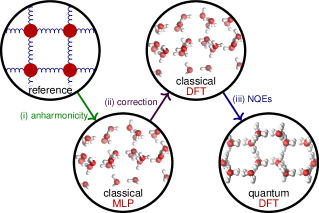
Figure 1: Thermodynamic integration steps from a reference system to the classical system described by the MLP, to the classical system described by DFT, and finally to the system with quantum-mechanical nuclei described by DFT.

II Results

Chemical potentials

For each ice structure, we first obtain the chemical potential over a temperature range of $25\text{\,}\mathrm{K}300\text{\,}\mathrm{K}$ and a pressure range of $0\text{\,}\mathrm{bar}10\,000\text{\,}\mathrm{bar}$ by performing classical free-energy calculations using the thermodynamic integration (TI) method as described in the Methods section. The MLP employed in these calculations is based on the hybrid revPBE0 Goerigk and Grimme (2011) functional with a semi-classical D3 dispersion correction Grimme et al. (2016). This MLP reproduces many properties of water, including the densities and the relative stabilities of I${}_{\text{h}}$, I${}_{\text{c}}$ and liquid water at the ambient pressure Cheng et al. (2019). Because the MLP is only trained on liquid water and not on either the structures or the energetics of the ice phases, it allows us to explore the ice phase diagram in an agnostic fashion. It nevertheless reproduces lattice energies, molar volume and phonon densities of states of diverse ice phases, since local atomic environments found in liquid water also cover those observed in the ice phases Monserrat et al. (2020).

The chemical potentials (expressed per molecule of H2O throughout this work) at $225\text{\,}\mathrm{K}$ computed using the MLP are reported in Fig. 2(a). Focussing only on the phases whose MLP chemical potential is within $10\text{\,}\mathrm{meV}$ of the ground-state phase under all conditions of interest, we narrow down the selection to 12 ice phases: ices I${}_{\text{h}}$, I${}_{\text{c}}$, II, III, V, VI, VII, IX, XI, XI${}_{\text{c}}$, XIII and XV, and the liquid. These phases are all known from experiment, which suggests that the experimental phase diagram of water is indeed complete Salzmann (2019). Moreover, as the chemical potential difference between I${}_{\text{h}}$ and I${}_{\text{c}}$ is small and has already been studied in Ref. Cheng et al. (2019), we report the results only for ‘ice I’.

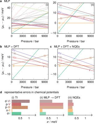
Figure 2: Per-molecule chemical potentials for the phases (meta)stable at $225\text{\,}\mathrm{K}$, shown relative to the chemical potential of ice II. The MLP results are in panel (a). In subpanel (i), solid lines show experimentally known bulk phases, dashed lines show various known low-density structures, and dotted lines show other hypothetical phases. Subpanel (ii) shows the same data, but only for the known experimental phases, as labelled. Panel (b) shows the chemical potentials at the level of the revPBE0-D3 DFT for classical systems, and panel (c) shows DFT results with NQE corrections. Panel (d) illustrates representative standard deviations for selected proton-disordered (‘d’), partially proton-disordered (‘p’) and proton-ordered (‘o’) phases. Contributions are split into those arising from (i) the thermodynamic integration to the classical system described by the MLP, with the contribution from proton disorder shown as a hatched area; (ii) the MLP to the revPBE0-D3 correction term; and (iii) the term accounting for NQEs.

The treatment of proton-disordered phases is complicated because choosing a non-representative configuration can introduce a significant bias in enthalpy and in turn lead to an incorrect phase diagram Conde et al. (2013). To overcome this, we use a combination of the Buch algorithm Buch et al. (1998) and GenIce Matsumoto et al. (2017) to generate 5–8 different depolarised proton-disordered manifestations of each disordered phase considered. For the partially proton-disordered phases III and V, we first construct many configurations, and then only consider the ones that match the experimental site occupancies Lobban et al. (2000). We compute the chemical potential of each such configuration independently and average over the results, and finally add a configurational entropy associated with (partial) proton disorder Herrero and Ramírez (2014); MacDowell et al. (2004).

We perform a free-energy perturbation to promote the MLP results to the hybrid DFT level (see revPBE0-D3 results in Fig. 2(b)), as detailed in the Methods section. This correction is necessary to recover the true chemical potential at the DFT level, because the MLP inevitably leads to small residual errors Behler (2015). Specifically, proton order leads to long-range electrostatics that can destabilise the solid, but the MLP only accounts for short-range interactions. Albeit small in absolute terms, the correction to DFT causes a changeover of stability, and in particular reduces the stability of the proton-ordered phases (such as ice II and XV), as can be seen from Fig. 2(b). Although the proton-ordered phases XI, XIII and XV are more stable than their proton-disordered analogues (I, V and VI, respectively) at the MLP level at low temperatures, at the DFT level, the proton order–disorder transition occurs at considerably lower temperatures than we focus on here, and so we do not characterise this transition further.

Finally, we consider NQEs by performing path-integral molecular dynamics (PIMD) simulations. In general, NQEs serve to stabilise higher-density phases. For all phases, the degree of stabilisation increases with increasing pressure, and decreases with increasing temperature. Whilst the overall form of the chemical potential plot [Fig. 2(c)] changes only subtly, NQEs can significantly shift the phase boundaries, and we return to this point below.

Although it is often difficult to determine error bars in free-energy calculations  Vega et al. (2008), we have estimated the errors arising from each step of the calculation (Fig. 2(d)) following the steps outlined in Subsect. IV.4. The uncertainty is small for the proton-ordered phases, but considerably larger for the proton-disordered phases, in which there are more varied local environments. The typical uncertainty in the chemical potential of each phase is at most $\sim$$2.5\text{\,}\mathrm{meV}$, but, as we show below, even this relatively small difference is often sufficient to change the coexistence lines significantly.

Phase diagram

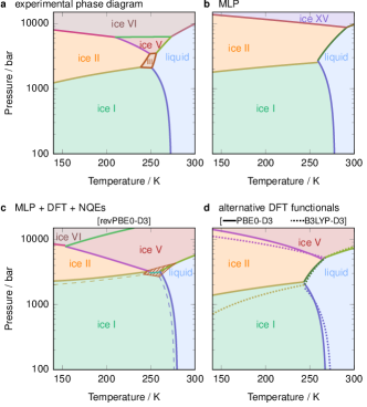
Figure 3: Phase diagrams (a) from experiment León et al. (2002); Wagner et al. (2011) and (b)–(d) from simulation. The phase diagram in panel (b) corresponds to the classical system described by the MLP, while panels (c) and (d) are at the indicated DFT levels and also account for NQE corrections. Dashed lines in panel (c) correspond to an alternative calculation where the chemical potential of ice III was decreased and that of ice I was increased by the typical error in chemical potential calculations (Fig. 2(d)), as discussed in the text. The hatched area corresponds to the region of stability of ice III in this alternative calculation.

We determine the phase diagram of water by analysing the computed chemical potentials over a wide range of pressure and temperature conditions. In Fig. 3, we show the phase diagram for the classical system described by the MLP, the ab initio phase diagram including NQEs, as well as the experimental phase diagram for comparison. Even just at the MLP level without NQEs, the phase diagram is already a reasonable approximation [Fig. 3(b)]. It captures the negative gradient of the pressure–temperature coexistence curve between ice I and liquid, but fails to account for ices III and V, and the proton-ordered XV is more stable than its disordered analogue (VI). As discussed above, the MLP is prone to overestimating the stability of the proton-ordered phases, which leads to this computational artefact.

When the MLP is corrected to the DFT level of theory and NQEs are accounted for, the resulting phase diagram [Fig. 3(c)] is considerably improved, and is in close agreement with experiment. Most of the stable phases appear, and the melting point of ice I at atmospheric pressure ($280\text{\,}\mathrm{K}$) agrees reasonably well with experiment. However, at very high pressure, the coexistence curve between ices V and VI has too steep a gradient compared to experiment. This may arise from the inaccuracy of the reference DFT functionals Gillan et al. (2016) or from the finite basis set and energy cutoffs employed in the DFT calculations. To illustrate the effect of employing different DFT approximations, we show analogous phase diagrams for two alternative DFT functionals, B3LYP-D3 and PBE0-D3, in Fig. 3(d). The melting points at $1\text{\,}\mathrm{bar}$, $274\text{\,}\mathrm{K}$ and $268\text{\,}\mathrm{K}$, respectively, are somewhat lower than for the revPBE0-D3 functional. Although the agreement of the melting point with experiment is very good for the B3LYP-D3 functional, this does not translate to the rest of the phase diagram.

In none of three phase diagrams shown in Fig. 3(c,d) is ice III thermodynamically stable. From the chemical potential results, we can see that ice III is within $\sim$$2\text{\,}\mathrm{meV}$ to the thermodynamically stable phase at pressures around $3000\text{\,}\mathrm{bar}$ and temperatures around $250\text{\,}\mathrm{K}$, where it is known to be stable from experiment. However, its chemical potential depends crucially on the particular manifestation of proton disorder that we choose, and to compute the chemical potentials of the proton-disordered ice phases, we average over a number of independent simulations with different initial proton-disorder configurations. As we have shown in Fig. 2(d), the typical error in computations associated with proton-disordered phases is about $2\text{\,}\mathrm{meV}$. To illustrate the extent to which such uncertainties affect the computed phase diagram, we show in Fig. 3(c) the phase diagram obtained when ice III is stabilised whilst ice I is destabilised, in each case by changing their chemical potentials by the standard deviation obtained from the above procedure. In such a scenario, ice III is stable over approximately the right range of temperatures and pressures. The main lessons to be drawn from this are that (i) many of the phases are very close in free energy, particularly in the region around $250\text{\,}\mathrm{K}$ and $\sim$$3000\text{\,}\mathrm{bar}$, which means that even if they are not thermodynamically stable, they are likely to be metastable and hence may be easier to obtain experimentally at these conditions, and (ii) the phase diagram is an extremely sensitive test of the underlying potential: even a very small change in relative stability can drastically affect the phase behaviour.

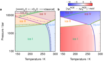
Figure 4: (a) Phase diagram excluding NQEs (dotted lines) alongside the full phase diagram (solid lines from Fig. 3(c)) and the phase diagram for D2O (dotted–dashed lines). (b) Heat map indicating the correction to the chemical potential of the stable phase $i$ due to NQEs, relative to ice II, overlaid on the phase diagram from Fig. 3(c).

Finally, we show the phase diagram with and without accounting for NQEs in Fig. 4(a). The NQE correction to the chemical potential of the most stable phase is shown in Fig. 4(b); we show the results relative to (metastable) ice II at the same pressure and temperature in order to remove the large effect of the dependence of the mean kinetic energy on the temperature. As we have already discussed, the addition of NQEs to the calculation stabilises the denser phases relative to the less dense ones: ice VI is more stabilised than ice V, ice V more than ice II, ice II more than the liquid, and the liquid more than ice I.

When NQEs are not accounted for, H2O and D2O exhibit exactly the same thermodynamic behaviour. However, accounting for the difference between them is necessary for example for polar ice dating and historical atmospheric temperature estimation Dreschhoff et al. (2020), which suggests that a classical description of nuclear motion is not satisfactory. We thus account for NQEs by integrating Eq. (2) to the mass of hydrogen or deuterium, to determine the phase behaviour of light and heavy water, respectively. We show the predicted phase diagram of H2O, D2O and ‘classical’ water (without NQEs) in Fig. 4(a). The melting point of ice I for H2O is approximately $4\text{\,}\mathrm{K}$ lower than that for D2O, as investigated previously Ramírez and Herrero (2010); Cheng et al. (2019). It is interesting thatD2O follows almost the same ice I–liquid coexistence line as classical water, since positive and negative contributions to the integral of Eq. (2) largely cancel out Cheng et al. (2019). A similar conclusion can be drawn about the coexistence line between ices I and II, perhaps because the density difference between the two phases is similar to that between ice I and the liquid. At higher pressures, however, the phase diagrams of H2O and D2O are drastically different from classical water, demonstrating the importance of properly accounting for NQEs.

III Conclusions

In this work, we have undertaken an exhaustive exploration of the phase diagram of water at three levels of hybrid DFT, including nuclear thermal fluctuations and proton disorder. The agreement between the computed and experimental phase diagrams is very good, but by no means perfect. Part of the difference can be explained in terms of the sensitivity to very small changes in the chemical potentials, which is particularly acute with proton-disordered phases. Furthermore, using DFT to model water, even at the hybrid level, has limitations Gillan et al. (2016). Finally, it is not guaranteed that the phases obtained in experiment are in fact the thermodynamically stable phases; as such, the experimental and the theoretical phase diagram may have subtle differences arising from slightly different definitions of phase stability. Nevertheless, the ab initio phase diagrams show a significant improvement over previous results based on empirical models Vega et al. (2005b); Wang et al. (2013), particularly at low pressure. Moreover, although NQEs are often neglected in the computation of the phase diagram of water, we have properly accounted for them in the present work. This allows us to characterise further the subtle difference between the phase behaviour of H2O and D2O.

Our entire calculation was premised on the fact that a MLP had been parameterised for water Cheng et al. (2019), which permitted the study of larger systems for sufficiently long to be able to compute their thermodynamic properties. While the DFT-level phase behaviour we have studied is the best we can do at this stage, for many applications, such as investigating the thermodynamics of the nucleation of ice, even the approach we have followed may not be computationally feasible. It would therefore be very tempting to use the inexpensive MLP on its own in future studies. From our results, we can conclude that, even though the potential was trained solely on liquid-phase structures, the description of the solid phases and the phase behaviour of the MLP on its own is very reasonable. However, a degree of care must be taken in interpreting its results, not least because proton-ordered phases are somewhat too stable when described by the MLP.

The good agreement between the calculated phase diagram and experiment confirms that the hybrid DFT levels of theory describe water well. In fact, the approach we have outlined to compute free energies and in turn phase diagrams provides a particularly difficult benchmark for quantum-mechanical methods. We have shown that three different hybrid DFT functionals (revPBE0-D3, PBE0-D3, B3LYP-D3) result in similar, but certainly not identical, phase behaviour. It would be interesting to apply the same workflow to other electronic structure methods, including random-phase approximation Langreth and Perdew (1977) and DFT at the double hybrid level Martin and Santra (2019). Indeed, in the future, one possible way of benchmarking and optimising DFT functionals may well be to evaluate the phase diagram of the material studied.

The present study bridges the gap between electronic structure theory and accurate computation of phase behaviour for water. The same framework can be used to investigate (meta)stability of novel bulk materials. It further lays the groundwork for utilising experimental phase diagrams to correct and improve interatomic potentials based on electronic structure methods.

IV Methods

IV.1 Candidate ice structures

We start from the 57 phases that were screened from an extensive set of 15,859 hypothetical ice structures using a generalised convex hull construction, an algorithm for identifying promising experimental candidates Anelli et al. (2018); Engel et al. (2018). We eliminate defected phases, dynamically unstable phases, and the very high pressure phase X, but add the originally missing ice IV. In the Supplementary Data, we provide the structures of the remaining 50 ice phases that we consider in our simulations.

IV.2 DFT calculations

We compute the energies of the water structures using the cp2k code Lippert et al. (1999) with the revPBE0-D3, the PBE0-D3 and the B3LYP-D3 functionals. The computational details of the calculations are identical to Ref. Cheng et al. (2019); Marsalek and Markland (2017) but for the choice of functionals, and we provide input files in the Supplementary Data.

IV.3 Free-energy calculations

We use the method of thermodynamic integration (TI) to compute the Gibbs energy of the selected ice phases at a wide range of thermodynamic conditions, which in turn determine the ice phase diagram. A similar method has previously been used to compute the ice phase diagram using empirical potentials Vega and Abascal (2011). In our approach, we use a series of steps in simulations of physical or artificial systems to compute the various components of the free-energy difference between a reference system and the fully anharmonic, quantum system, as depicted schematically in Fig. 1.

In the first step of the free-energy calculation for the solid phases, we equilibrate a sample of an ice phase at the temperature and pressure of interest in an isothermal-isobaric simulation with a fluctuating box with a Parrinello–Rahman-like barostat Parrinello and Rahman (1981) to determine the equilibrium lattice parameters at the conditions of interest. We then prepare a perfect crystal with the corresponding lattice parameters and minimise its energy, compute the Helmholtz energy of the reference harmonic crystal by determining the eigenvalues of the hessian matrix, account for the motion of the centre of mass, and finally perform a thermodynamic integration step to the potential of interest in which classical nuclei are described by the MLP [Fig. 1(i)]. By adding a suitable pressure–volume term, we obtain the fully anharmonic classical chemical potential of the ice system described by the MLP. The details of this procedure are discussed in Ref. 57. In this step, we use reasonably large system sizes (of the order a few hundred to several thousand water molecules) to ensure that finite-size effects are minimised. Determining the chemical potential in this way would have been computationally intractable had we employed ab initio calculations, and is only made possible by the use of the MLP. Once the chemical potential is known for the MLP at one set of conditions, we can find it at other pressures and temperatures by numerically integrating the Gibbs–Duhem relation along isotherms and the Gibbs-energy analogue of the Gibbs–Helmholtz relations along isobars, respectively.

To find the free energy of the liquid phase at the MLP level, we perform a series of direct-coexistence simulations Opitz (1974); Vega et al. (2008) of the liquid in contact with ice I${}_{\text{h}}$ at a series of temperatures at $0\text{\,}\mathrm{bar}$ to determine the coexistence temperature. The melting point $T_{\text{m}}=$279.5\text{\,}\mathrm{K}$$ at $1\text{\,}\mathrm{bar}$ for the MLP, although evaluated in a different way, is in perfect agreement with a previous simulation that used umbrella sampling Cheng et al. (2019). We equate the chemical potentials of the two phases under these conditions and obtain the chemical potential of the liquid at other conditions by thermodynamic integration along isotherms and isobars, as for the ice phases.

In the second step of the procedure [Fig. 1(ii)], we promote the chemical potential of the system as described by the MLP to the DFT potential-energy surface level of theory using a free-energy perturbation,

$$\upDelta\mu^{\mathrm{MLP\to DFT}}(P,\,T)=-\dfrac{k_{\text{B}}T}{N}\ln\left\langle\exp\left[-\frac{U_{\text{DFT}}-U_{\text{ML}}}{k_{\text{B}}T}\right]\right\rangle_{P,T,\mathcal{H}_{\text{ML}}}\,,$$ (1)

where $\left\langle\cdot\right\rangle_{P,T,\mathcal{H}_{\text{ML}}}$ denotes the ensemble average of the system sampled at temperature $T$ and pressure $P$ using the ML hamiltonian $\mathcal{H}_{\text{ML}}$, where $U_{\text{DFT}}$ is the DFT energy and $U_{\text{ML}}$ is the MLP energy, and $N$ is the number of water molecules in the system. This correction is necessary to recover the true chemical potential at the DFT level, in particular to compensate for the lack of long-range electrostatics, which are particularly important in modulating ice phase stabilities Melko et al. (2001). Using the MLP-derived chemical potentials without corrections neglects such long-range contributions and significantly hampers the quantitative accuracy of the computed phase diagram. In practice, we first collect trajectories of ice configurations by performing MD simulations in the isothermal-isobaric ensemble for each promising ice phase using the MLP. The number of water molecules in the simulation cell ranges from 56 to 96 molecules, depending on the unit-cell size of each phase. For each of the proton-disordered (I, VI) or partially disordered phases (III, V), we run independent simulations for 5–8 different depolarised proton-disordered configurations. We then select decorrelated configurations from the MD trajectories and recompute their energies at the DFT level. The MLP $\to$ DFT correction terms are then computed using Eq. (1) and averaged over the different disordered structures for the proton-disordered phases.

In this step, the correction to the chemical potential ranges from $-7.9\text{\,}\mathrm{meV}$ (for ice VI at $125\text{\,}\mathrm{K}$ and $10\,000\text{\,}\mathrm{bar}$) to $10.8\text{\,}\mathrm{meV}$ (for ice XV at $275\text{\,}\mathrm{K}$ and $5000\text{\,}\mathrm{bar}$). Ice XV is the proton-ordered analogue of ice VI; similarly, ice XIII, the proton-ordered analogue of ice V, is more stable at the MLP level than it ought to be [e.g. at $225\text{\,}\mathrm{K}$ and $7000\text{\,}\mathrm{bar}$, the corrections to chemical potentials are $\upDelta\mu_{\text{V}}=$-1.5\text{\,}\mathrm{meV}$$ and $\upDelta\mu_{\text{XIII}}=$3.4\text{\,}\mathrm{meV}$$]. Indeed the difference in the correction term between these two pairs of phases is largely insensitive to temperature and pressure, at least at the pressures where the phases are competitive and for which we have computed the correction reliably; namely, $\upDelta\upDelta\mu(\text{V}\to\text{XIII})\approx$5\text{\,}\mathrm{meV}$$ and $\upDelta\upDelta\mu(\text{VI}\to\text{XV})\approx$11\text{\,}\mathrm{meV}$$.

During the final TI [Fig. 1(iii)], NQEs are taken into account by integrating the quantum centroid virial kinetic energy $\left\langle E_{\text{k}}\right\rangle$ with respect to the fictitious ‘atomic’ mass $\tilde{m}$ from the classical (i.e. infinite) mass to the physical masses $m$ Ramírez and Herrero (2010); Ceriotti and Markland (2013); Cheng et al. (2016); Cheng and Ceriotti (2014); Cheng et al. (2018). In practice, a change of variable $y=\sqrt{m/\tilde{m}}$ is applied to reduce the discretisation error in the evaluation of the integral Ceriotti and Markland (2013), yielding

$$\upDelta\mu^{\text{NQE}}(P,\,T)=2\int_{0}^{1}\frac{\left\langle E_{\text{k}}(1/y^{2})\right\rangle}{y}\,\mathrm{d}y.$$ (2)

We evaluate the integrand using PIMD simulations for $y=1/4$, $1/2$, $\sqrt{2}/2$ and 1, and then numerically integrate it. In these PIMD simulations, we use 24 beads for all phases considered at a wide range of constant pressure and temperature conditions for $T\geq$125\text{\,}\mathrm{K}$$. Relative to ice II, the correction to the chemical potential arising from NQEs ranges from $-8\text{\,}\mathrm{meV}$ to $5\text{\,}\mathrm{meV}$.

IV.4 Uncertainty estimation

To determine the approximate uncertainty associated with the individual chemical potential contributions, we first compute the reference chemical potential of several phases computed from an equilibrated perfect crystal at $125\text{\,}\mathrm{K}$ and $0\text{\,}\mathrm{bar}$. We repeat this calculation between 5 and 10 times and determine the standard deviation of the resulting chemical potentials. For (partially and fully) proton-disordered phases, we split the contributions to the standard deviation arising from thermodynamic integration, which we obtain by computing the reference chemical potential calculation using the same initial configuration in 5 independent simulations, and from proton disorder, which we obtain by averaging over the chemical potentials arising from several distinct manifestations of the proton disorder in the initial configurations. Similarly, we compute the standard deviation of the correction to the chemical potential when the system is integrated from the MLP to the DFT level evaluated at $225\text{\,}\mathrm{K}$ and $3000\text{\,}\mathrm{bar}$. For the correction to NQEs, we determine the statistical error in the measurement of the kinetic energy at each scaled mass. We calculate the integral of Eq. (2) with an analogue of Simpson’s rule for irregularly spaced data both for the mean values as well as the mean value increased by the standard deviation, and we estimate the a posteriori NQE error to be the difference between these two corrections.

References

- Debenedetti (2003) P. G. Debenedetti, “Supercooled and glassy water,” J. Phys.: Condens. Matter 15, R1669 (2003).
- Salzmann (2019) C. G. Salzmann, “Advances in the experimental exploration of water’s phase diagram,” J. Chem. Phys. 150, 060901 (2019).
- Vega et al. (2009) C. Vega, J. L. F. Abascal, M. M. Conde, and J. L. Aragones, “What ice can teach us about water interactions: A critical comparison of the performance of different water models,” Faraday Discuss. 141, 251 (2009).
- Vega and Abascal (2011) C. Vega and J. L. F. Abascal, “Simulating water with rigid non-polarizable models: A general perspective,” Phys. Chem. Chem. Phys. 13, 19663 (2011).
- Noya et al. (2007) E. G. Noya, C. Menduiña, J. L. Aragones, and C. Vega, “Equation of state, thermal expansion coefficient, and isothermal compressibility for ices I, II, III, V, and VI, as obtained from computer simulation,” J. Phys. Chem. C 111, 15877 (2007).
- Abascal et al. (2009) J. L. F. Abascal, E. Sanz, and C. Vega, “Triple points and coexistence properties of the dense phases of water calculated using computer simulation,” Phys. Chem. Chem. Phys. 11, 556 (2009).
- Agarwal et al. (2011) M. Agarwal, M. P. Alam, and C. Chakravarty, “Thermodynamic, diffusional, and structural anomalies in rigid-body water models,” J. Phys. Chem. B 115, 6935 (2011).
- Conde et al. (2013) M. M. Conde, M. A. Gonzalez, J. L. F. Abascal, and C. Vega, “Determining the phase diagram of water from direct coexistence simulations: The phase diagram of the TIP4P/2005 model revisited,” J. Chem. Phys. 139, 154505 (2013).
- Quigley and Rodger (2008) D. Quigley and P. M. Rodger, “Metadynamics simulations of ice nucleation and growth,” J. Chem. Phys. 128, 154518 (2008).
- Reinhardt et al. (2012) A. Reinhardt, J. P. K. Doye, E. G. Noya, and C. Vega, “Local order parameters for use in driving homogeneous ice nucleation with all-atom models of water,” J. Chem. Phys. 137, 194504 (2012).
- Reinhardt and Doye (2013) A. Reinhardt and J. P. K. Doye, “Note: Homogeneous TIP4P/2005 ice nucleation at low supercooling,” J. Chem. Phys. 139, 096102 (2013).
- Malkin et al. (2012) T. L. Malkin, B. J. Murray, A. V. Brukhno, J. Anwar, and C. G. Salzmann, “Structure of ice crystallized from supercooled water,” Proc. Natl. Acad. Sci. U. S. A. 109, 1041 (2012).
- Espinosa et al. (2014) J. R. Espinosa, E. Sanz, C. Valeriani, and C. Vega, “Homogeneous ice nucleation evaluated for several water models,” J. Chem. Phys. 141, 18C529 (2014).
- Jorgensen et al. (1983) W. L. Jorgensen, J. Chandrasekhar, J. D. Madura, R. W. Impey, and M. L. Klein, “Comparison of simple potential functions for simulating liquid water,” J. Chem. Phys. 79, 926 (1983).
- Rick (2004) S. W. Rick, “A reoptimization of the five-site water potential (TIP5P) for use with Ewald sums,” J. Chem. Phys. 120, 6085 (2004).
- Abascal and Vega (2005) J. L. F. Abascal and C. Vega, “A general purpose model for the condensed phases of water: TIP4P/2005,” J. Chem. Phys. 123, 234505 (2005).
- Berendsen et al. (1987) H. J. C. Berendsen, J. R. Grigera, and T. P. Straatsma, “The missing term in effective pair potentials,” J. Phys. Chem. 91, 6269 (1987).
- Habershon and Manolopoulos (2011a) S. Habershon and D. E. Manolopoulos, “Thermodynamic integration from classical to quantum mechanics,” J. Chem. Phys. 135, 224111 (2011a).
- Habershon and Manolopoulos (2011b) S. Habershon and D. E. Manolopoulos, “Free energy calculations for a flexible water model,” Phys. Chem. Chem. Phys. 13, 19714 (2011b).
- Habershon et al. (2009) S. Habershon, T. E. Markland, and D. E. Manolopoulos, “Competing quantum effects in the dynamics of a flexible water model,” J. Chem. Phys. 131, 024501 (2009).
- McBride et al. (2009) C. McBride, C. Vega, E. G. Noya, R. Ramírez, and L. M. Sesé, “Quantum contributions in the ice phases: The path to a new empirical model for water—TIP4PQ/2005,” J. Chem. Phys. 131, 024506 (2009).
- McBride et al. (2012) C. McBride, E. G. Noya, J. L. Aragones, M. M. Conde, and C. Vega, “The phase diagram of water from quantum simulations,” Phys. Chem. Chem. Phys. 14, 10140 (2012).
- Reddy et al. (2016) S. K. Reddy, S. C. Straight, P. Bajaj, C. H. Pham, M. Riera, D. R. Moberg, M. A. Morales, C. Knight, A. W. Götz, and F. Paesani, “On the accuracy of the MB-pol many-body potential for water: Interaction energies, vibrational frequencies, and classical thermodynamic and dynamical properties from clusters to liquid water and ice,” J. Chem. Phys. 145, 194504 (2016).
- Wang et al. (2013) L.-P. Wang, T. Head-Gordon, J. W. Ponder, P. Ren, J. D. Chodera, P. K. Eastman, T. J. Martinez, and V. S. Pande, “Systematic improvement of a classical molecular model of water,” J. Phys. Chem. B 117, 9956 (2013).
- Vega et al. (2005a) C. Vega, E. Sanz, and J. L. F. Abascal, “The melting temperature of the most common models of water,” J. Chem. Phys. 122, 114507 (2005a).
- Vega et al. (2005b) C. Vega, J. L. F. Abascal, E. Sanz, L. G. MacDowell, and C. McBride, “Can simple models describe the phase diagram of water?” J. Phys.: Condens. Matter 17, S3283 (2005b).
- Deringer et al. (2019) V. L. Deringer, M. A. Caro, and G. Csányi, “Machine learning interatomic potentials as emerging tools for materials science,” Adv. Mater. 31, 1902765 (2019).
- Morawietz et al. (2016) T. Morawietz, A. Singraber, C. Dellago, and J. Behler, “How van der Waals interactions determine the unique properties of water,” Proc. Natl. Acad. Sci. U. S. A. 113, 8368 (2016).
- Cheng et al. (2019) B. Cheng, E. A. Engel, J. Behler, C. Dellago, and M. Ceriotti, “Ab initio thermodynamics of liquid and solid water,” Proc. Natl. Acad. Sci. U. S. A. 116, 1110 (2019).
- Niu et al. (2020) H. Niu, L. Bonati, P. M. Piaggi, and M. Parrinello, “Ab initio phase diagram and nucleation of gallium,” Nat. Commun. 11, 2654 (2020).
- Cheng et al. (2020) B. Cheng, G. Mazzola, C. J. Pickard, and M. Ceriotti, “Evidence for supercritical behaviour of high-pressure liquid hydrogen,” Nature 585, 217 (2020).
- Pauling (1935) L. Pauling, “The structure and entropy of ice and of other crystals with some randomness of atomic arrangement,” J. Am. Chem. Soc. 57, 2680 (1935).
- Bernal and Fowler (1933) J. D. Bernal and R. H. Fowler, “A theory of water and ionic solution, with particular reference to hydrogen and hydroxyl ions,” J. Chem. Phys. 1, 515 (1933).
- Herrero and Ramírez (2014) C. P. Herrero and R. Ramírez, “Configurational entropy of hydrogen-disordered ice polymorphs,” J. Chem. Phys. 140, 234502 (2014).
- MacDowell et al. (2004) L. G. MacDowell, E. Sanz, C. Vega, and J. L. F. Abascal, “Combinatorial entropy and phase diagram of partially ordered ice phases,” J. Chem. Phys. 121, 10145 (2004).
- Goerigk and Grimme (2011) L. Goerigk and S. Grimme, “A thorough benchmark of density functional methods for general main group thermochemistry, kinetics, and noncovalent interactions,” Phys. Chem. Chem. Phys. 13, 6670 (2011).
- Grimme et al. (2016) S. Grimme, A. Hansen, J. G. Brandenburg, and C. Bannwarth, “Dispersion-corrected mean-field electronic structure methods,” Chem. Rev. 116, 5105 (2016).
- Monserrat et al. (2020) B. Monserrat, J. G. Brandenburg, E. A. Engel, and B. Cheng, “Extracting ice phases from liquid water: why a machine-learning water model generalizes so well,” arXiv preprint arXiv:2006.13316 (2020).
- Buch et al. (1998) V. Buch, P. Sandler, and J. Sadlej, “Simulations of \ceH2O solid, liquid, and clusters, with an emphasis on ferroelectric ordering transition in hexagonal ice,” J. Phys. Chem. B 102, 8641 (1998).
- Matsumoto et al. (2017) M. Matsumoto, T. Yagasaki, and H. Tanaka, “GenIce: Hydrogen-disordered ice generator,” J. Comput. Chem. 39, 61 (2017).
- Note (1) We have assumed that the experimental proton disorder is correct for the potential used, which may not be completely accurate Conde et al. (2013), but is the best possible assumption we can make, since equilibration of proton disorder is not feasible to achieve on computationally tractable time scales.
- Lobban et al. (2000) C. Lobban, J. L. Finney, and W. F. Kuhs, “The structure and ordering of ices III and V,” J. Chem. Phys. 112, 7169 (2000).
- Behler (2015) J. Behler, “Constructing high-dimensional neural network potentials: A tutorial review,” Int. J. Quantum Chem. 115, 1032 (2015).
- Vega et al. (2008) C. Vega, E. Sanz, J. L. F. Abascal, and E. G. Noya, “Determination of phase diagrams via computer simulation: Methodology and applications to water, electrolytes and proteins,” J. Phys.: Condens. Matter 20, 153101 (2008).
- León et al. (2002) G. León, S. R. Romo, and V. Tchijov, “Thermodynamics of high-pressure ice polymorphs: ice II,” J. Phys. Chem. Solids 63, 843 (2002).
- Wagner et al. (2011) W. Wagner, T. Riethmann, R. Feistel, and A. H. Harvey, “New equations for the sublimation pressure and melting pressure of \ceH2O ice I,” J. Phys. Chem. Ref. Data 40, 43103 (2011).
- Gillan et al. (2016) M. J. Gillan, D. Alfè, and A. Michaelides, “Perspective: How good is DFT for water?” J. Chem. Phys. 144, 130901 (2016).
- Dreschhoff et al. (2020) G. Dreschhoff, H. Jungner, and C. M. Laird, “Deuterium–hydrogen ratios, electrical conductivity and nitrate for high-resolution dating of polar ice cores,” Tellus B Chem. Phys. Meteorol. 72, 1 (2020).
- Ramírez and Herrero (2010) R. Ramírez and C. P. Herrero, “Quantum path integral simulation of isotope effects in the melting temperature of ice Ih,” J. Chem. Phys. 133, 144511 (2010).
- Langreth and Perdew (1977) D. C. Langreth and J. P. Perdew, “Exchange-correlation energy of a metallic surface: Wave-vector analysis,” Phys. Rev. B 15, 2884 (1977).
- Martin and Santra (2019) J. M. L. Martin and G. Santra, “Empirical double-hybrid density functional theory: A ‘third way’ in between WFT and DFT,” Isr. J. Chem. 60, 787 (2019).
- Anelli et al. (2018) A. Anelli, E. A. Engel, C. J. Pickard, and M. Ceriotti, “Generalized convex hull construction for materials discovery,” Phys. Rev. Materials 2, 103804 (2018).
- Engel et al. (2018) E. A. Engel, A. Anelli, M. Ceriotti, C. J. Pickard, and R. J. Needs, “Mapping uncharted territory in ice from zeolite networks to ice structures,” Nat. Commun. 9, 2173 (2018).
- Lippert et al. (1999) G. Lippert, J. Hutter, and M. Parrinello, “The Gaussian and augmented-plane-wave density functional method for ab initio molecular dynamics simulations,” Theor. Chem. Acc. 103, 124 (1999).
- Marsalek and Markland (2017) O. Marsalek and T. E. Markland, “Quantum dynamics and spectroscopy of ab initio liquid water: The interplay of nuclear and electronic quantum effects,” J. Phys. Chem. Lett. 8, 1545 (2017).
- Parrinello and Rahman (1981) M. Parrinello and A. Rahman, “Polymorphic transitions in single crystals: A new molecular dynamics method,” J. Appl. Phys. 52, 7182 (1981).
- Cheng and Ceriotti (2018) B. Cheng and M. Ceriotti, “Computing the absolute Gibbs free energy in atomistic simulations: Applications to defects in solids,” Phys. Rev. B 97, 054102 (2018).
- Opitz (1974) A. C. L. Opitz, “Molecular dynamics investigation of a free surface of liquid argon,” Phys. Lett. A 47, 439 (1974).
- Melko et al. (2001) R. G. Melko, B. C. den Hertog, and M. J. Gingras, “Long-range order at low temperatures in dipolar spin ice,” Phys. Rev. Lett. 87, 067203 (2001).
- Ceriotti and Markland (2013) M. Ceriotti and T. E. Markland, “Efficient methods and practical guidelines for simulating isotope effects,” J. Chem. Phys. 138, 014112 (2013).
- Cheng et al. (2016) B. Cheng, J. Behler, and M. Ceriotti, “Nuclear quantum effects in water at the triple point: Using theory as a link between experiments,” J. Phys. Chem. Lett. 7, 2210 (2016).
- Cheng and Ceriotti (2014) B. Cheng and M. Ceriotti, “Direct path integral estimators for isotope fractionation ratios,” J. Chem. Phys. 141, 244112 (2014).
- Cheng et al. (2018) B. Cheng, A. T. Paxton, and M. Ceriotti, “Hydrogen diffusion and trapping in -iron: The role of quantum and anharmonic fluctuations,” Phys. Rev. Lett. 120, 225901 (2018).