PPQ-Trajectory: Spatio-temporal Quantization for Querying in Large Trajectory Repositories

Abstract.

We present PPQ-trajectory, a spatio-temporal quantization based solution for querying large dynamic trajectory data. PPQ-trajectory includes a partition-wise predictive quantizer (PPQ) that generates an error-bounded codebook with autocorrelation and spatial proximity-based partitions. The codebook is indexed to run approximate and exact spatio-temporal queries over compressed trajectories. PPQ-trajectory includes a coordinate quadtree coding for the codebook with support for exact queries. An incremental temporal partition-based index is utilised to avoid full reconstruction of trajectories during queries. An extensive set of experimental results for spatio-temporal queries on real trajectory datasets is presented. PPQ-trajectory shows significant improvements over the alternatives with respect to several performance measures, including the accuracy of results when the summary is used directly to provide approximate query results, the spatial deviation with which spatio-temporal path queries can be answered when the summary is used as an index, and the time taken to construct the summary. Superior results on the quality of the summary and the compression ratio are also demonstrated.

PVLDB Reference Format:
PVLDB, 14(2): 215-227, 2021.
doi:10.14778/3425879.3425891

1. Introduction

With the prevalence of positioning devices and mobile services, massive amounts of location sequences are being generated continuously. Maintaining and querying small-sized representations of raw trajectory data are needed for a wide variety of applications, such as real-time traffic management (ning2019vehicular) and intelligent transport systems (cai2017vector).

Existing trajectory compression methods do not address this need for a number of reasons. First, many of them are defined for edge sequences in a road network (funke2019pathfinder; han2017compress; koide2018enhanced; song2014press). They require pre-processing steps of mapping raw GPS data to the road network structure, followed by transforming the map-matched location data to edge-based sequences. The mapping and transformation processes reduce accuracy and result in limited support for detailed queries. Second, most solutions perform offline compression over full trajectory data, with execution times usually undesirable for online applications. There is a need for scalable online compression. Third, the existing compressed representations can not be directly used to answer spatio-temporal queries without a costly decompression process.

To address these challenges, we present PPQ-trajectory, a spatio-temporal quantization-based solution to generate a compact representation and support a wide range of queries over large trajectory data. An overview of PPQ-trajectory is presented in Figure 1.

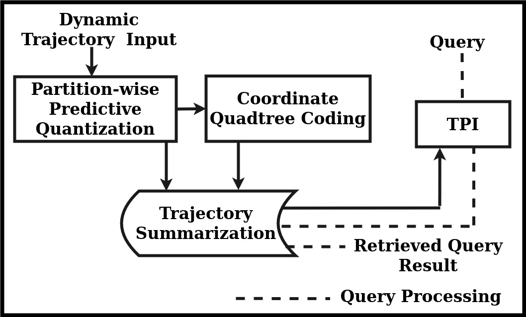
Figure 1. An Overview of PPQ-trajectory

The first part of PPQ-trajectory is the partition-wise predictive quantizer (PPQ) that generates an error-bounded summary, consisting of the codebook and prediction coefficients for spatial and autocorrelation-based partitions. The second part is the coordinate quadtree coding (CQC) for the error space caused by the quantization, which enables an accurate reconstruction of the trajectories. These two parts form the summary for the trajectory data, as illustrated in Figure 1. The third part is the temporal partition-based index (TPI) for organizing the quantized spatio-temporal data. Given a query, TPI is used to prune the data space and generate a candidate list of trajectories, whose reconstructed points can be computed from the summary. Overall, PPQ-trajectory generates and uses an indexed summary over raw data sequences to support efficient analysis, ranging from simple queries, such as vehicles passing by a location $(x,y)$ at a given time $t$, to more complex analytic tasks, such as predicting future positions of entities.

We evaluate PPQ-trajectory with respect to a number of performance measures: the quality of approximate query results, efficiency of exact queries, index building times, and compression ratio. We implemented several baselines, including the widely-used product quantization (jegou2010product), residual quantization (chen2010approximate), REST (zhao2018rest), which is a recent reference based trajectory compression method, and TrajStore (cudre2010trajstore), an adaptive storage solution for trajectories.

This paper makes the following contributions: (1) A spatio-temporal predictive quantizer, PPQ, is designed with an error-bounded codebook for each of the partitions, which are incrementally generated based on spatial and autocorrelation similarity. (2) Utilizing a quadtree structure and a padding process, CQC is developed to encode the relative positions of trajectory points with reconstructed ones for an accurate trajectory reconstruction. A local search strategy is presented to identify exact query results. (3) The temporal partition-based index dynamically reuses parts of the past index to support efficient spatio-temporal queries. (4) PPQ-trajectory answers spatio-temporal queries over raw data, without a full reconstruction of trajectories or accessing all of the candidate trajectories. (5) Experimental results demonstrate significant improvements achieved by PPQ-trajectory. For example, for approximate spatio-temporal queries, it is $3\%-52\%$ more accurate, compared to product quantization, residual quantization, and TrajStore. The mean absolute error (MAE) of PPQ-trajectory is a few or tens of meters, while the alternative approaches’ MAE values are orders of magnitude larger for the same size codebook. Significant improvements are also observed for the efficiency, index building times, and compression ratios.

The rest of the paper is organized as follows. The related work is in Section 2. Section 3 presents PPQ. In Section LABEL:optimal_solution, we present CQC and the associated local search strategy. In Section LABEL:TSDI, the temporal organization for the quantized data is presented. The effectiveness of PPQ-trajectory is verified via an extensive set of experiments in Section LABEL:experiments. Conclusion is provided in Section LABEL:conclusion.

2. Related Work

With the widespread adoption of location-based services, compressing trajectory data has become a prevalent area with high practical relevance (bellman2015applied; koide2018enhanced; liu2016novel). While traditional compression methods aim to reduce the reconstruction error and improve compression ratio, the data management challenge is to design the compression method with the objective of answering queries efficiently, and supporting online querying directly over compressed data.

Road network-constrained trajectory compression has gained significant attention (funke2019pathfinder; han2017compress; koide2018enhanced; liu2015bounded; popa2015spatio; song2014press). The common approach is to map raw trajectories to road networks and compress the map-matched trajectories (kellaris2013map). There is also significant attention on raw trajectory compression. SQUISH and SQUISH-E use a priority queue to remove redundant points (muckell2011squish; muckell2014compression). A bounded quadrant system (BQS) is developed in (liu2015bounded), which uses convex hull bounding to achieve trajectory compression. Based on BQS, (liu2016novel) achieves streaming trajectory compression, and aging history data without overwriting. Another recent method transforms trajectories into vehicle state vector functions and generates an inverted index based on the road segments (cai2017vector). This approach requires road segment information and matching each road id with corresponding objects.

The solutions that we included in our experiments are TrajStore (cudre2010trajstore) and REST (zhao2018rest). TrajStore aims compression via an adaptive spatial index and clustering the sub-trajectories. It recursively updates the index by merging, splitting or appending. REST is a recent compression-based method which compares trajectories with the sub-trajectories of a reference set. Generating a representative set is challenging especially under changing conditions, where it can fail to represent data from regions that lack enough samples.

Early work in this area applies traditional index structures for trajectory data. For example, STRIPES uses quadtrees to index the predicted positions of moving objects (patel2004stripes). In (cai2004indexing), an index for trajectories is developed by indexing the coefficients of Chebyshev polynomials that represent trajectories. Most those methods focus on similarity queries and do not address efficient spatio-temporal database queries. Zheng et al., (zheng2019reference) index the reference-based trajectories with IR-tree (li2010ir), which is based on R-tree referring to the inverted files for sub-trajectories.

Quantization is a popular method for traditional compression, and for nearest neighbor searches on multi dimensional data, especially for multimedia and computer vision applications (ferhatosmanoglu2000vector; liu2003efficient; norouzi2013cartesian; tuncel2002vq; weber1998quantitative). Predictive quantization has been applied for online summarization of multiple one-dimensional data streams (altiparmak2007incremental). The correlation among consecutive points is employed to predict current points, then the prediction errors are summarized into a smaller number of bits (altiparmak2007incremental). Product Quantization and Residual Quantization (chen2010approximate; ge2013optimized; jegou2010product) have made significant impact on approximate nearest neighbor searching in computer vision applications. We included these two methods in our performance evaluation. There have been some work to use quantization for encoding trajectories (chen2012compression), transforming differential trajectory points into strings for compression (lv2015trajectory), and retaining information for trajectory prediction (chan2012utilizing). These methods adopt compression but with no particular support for efficient querying over compressed trajectories. Our goal is to quantize dynamic trajectories into an error-bounded and query friendly representation, where there is neither need to fully reconstruct nor traverse the full trajectories. Trajectory data is summarized online, exploiting their large-scale nature, for the purpose of efficient query processing.

3. Online Quantization in
PPQ-Trajectory

In this section, we present our spatio-temporal quantization based summarization process. The performance measures are the accuracy of results when the summary is used directly to provide approximate query results, the spatial deviation with which spatio-temporal path queries can be answered when the summary is used as an index, and the time taken to construct the summary. The quality of the summary and the compression ratio are also related measures. Table 1 summarizes the notation used throughout the paper. Basic definitions of trajectories and codebooks are as follows.

Definition 3.1.

(Trajectory) A trajectory $T$ is a finite sequence of time-stamped positions in the form of (($x_{1}$, $y_{1}$, $t_{1}$), ($x_{2}$, $y_{2}$, $t_{2}$), …, ($x_{n}$, $y_{n}$, $t_{n}$)), where $0\leq t_{i}\leq t_{j}\leq t_{n}$ with $0\leq i\leq j\leq n$.

Definition 3.2.

(Error-bounded Codebook) Consider a codebook $C$ = $\{C_{1},...,C_{n}\}$ where the set of trajectory points $\mathcal{T}^{i}$ is indexed by codeword $C_{i}$. For any trajectory point $T_{j}^{t}\in\mathcal{T}^{i}$, if $\left\|T_{j}^{t}-C_{i}\right\|_{2}$ $\leq$ $\varepsilon_{1}$, then the codebook $C$ is bounded with $\varepsilon_{1}$.

Table 1. Summary of Notation

Variable	Definition
$T_{i}$	the $i$-th trajectory
$T_{i}^{t}$	trajectory point of $T_{i}$ at time $t$
$T^{t}$	trajectory points at time $t$
$\widehat{T}_{i}^{t}$	reconstructed trajectory point of $T_{i}^{t}$
$\widetilde{T}_{i}^{t}$	predicted trajectory point of $T_{i}^{t}$
$e_{i}^{t}$	prediction error of $T_{i}^{t}$, i.e., $T_{i}^{t}-\tilde{T}_{i}$
$f$	a prediction function
$C$	error bounded codebook
$b_{i}^{t}$	codeword index for $e_{i}^{t}$
$\varepsilon_{1}$	spatial deviation threshold
$\varepsilon_{1}^{M}$	$\varepsilon_{1}$ under the geographic coordinate system
$\varepsilon_{p}$	partition threshold for PPQ
$\varepsilon_{s}$	partition threshold for constructing index
${{{\hat{T_{i}}}^{t}}^{\prime}}$	reconstruction of ${T_{i}}^{t}$ considering CQC

3.1. Error-bounded Predictive Quantization

We first present the error bounded predictive quantizer (E-PQ) to obtain a compact codebook for trajectories. Predictive quantization (PQ) has been successfully applied for one-dimensional data streams by quantizing the error of the estimate of the sample at time $t$ with previous $k$ samples, i.e., $\widetilde{x}[t]=f(x[t-1],x[t-2],...,x[t-k])$ (altiparmak2007incremental; fletcher2007robust). A prediction function $f$ is learned over training data, and a codebook is generated via a vector quantizer (tuncel2002vq) on the prediction errors by assigning them to the nearest centroids of their clusters. The range of the error $e[t]=x[t]-\widetilde{x}[t]$ is narrower than the original data which enables the errors to be quantized more effectively than the original data (altiparmak2007incremental).

To estimate the trajectory points using their correlations, we define a prediction function as an extension to the case for one-dimensional streams (altiparmak2007incremental). For ease of demonstration, we define $f$ as a linear model that predicts ${T}^{t}_{i}$ using the previous $k$ samples. The prediction is computed as:

(1) $$\underset{f}{\text{min}}\sum_{i=1}^{N}\left\|{T}^{t}_{i}-f({T}^{(t-k:t-1)}_{i})\right\|_{2}$$

where $T^{t}_{i}$ represents the position $(x_{t},y_{t})$ of $T_{i}$ at time $t$, ${T}^{(t-k:t-1)}_{i}$ is the sequence of the trajectory $T_{i}$ at time interval $[t-k,t-1]$, and $f$ denotes the prediction model.

The prediction error $e^{t}_{i}$ is defined as:

(2) $$e^{t}_{i}=T^{t}_{i}-\widetilde{T}^{t}_{i}, \widetilde{T}^{t}_{i}=\sum_{j=1}^{k}P_{j}[t]\widehat{T}^{{t-j}}_{i}$$

where $\widetilde{T}^{t}_{i}$ is the prediction of $T^{t}_{i}$, $P_{j}[t]$ is the $j$-th prediction coefficient of $f$, and $\widehat{T}^{{t-k}}_{i}$ is the reconstruction of ${T}^{{t-k}}_{i}$.

The prediction errors $\{e^{t}_{i}\}$ can be summarized into an error-bounded codebook $C$ as:

(3) $$\quad\quad\quad\quad\text{min}|C|$$

$$\text{s.t.}{\left\|e^{t}_{i}-C(b^{t}_{i})\right\|_{2}}\leq\varepsilon_{1},b^{t}_{i}\in\{1,...,V\}$$

where $C=\{C_{1},C_{2},...,C_{V}\}$ is the error-bounded codebook, $V$ denotes the size of $C$, $b^{t}_{i}$ is the codeword index for $e_{i}^{t}$, and $C(b^{t}_{i})$ denotes the codeword assigned to represent $e^{t}_{i}$. Every codeword $C_{i}\in C$ is a cluster centroid, obtained by partitioning the data space to facilitate indexing and compression. Equation LABEL:eq:r3 aims to achieve a minimal error-bounded codebook $C$ for the given $\varepsilon_{1}$, which is non-convex. For dynamic databases, $C$ needs to be incrementally updated with evolving $t$ values. In order to get the approximate solution, at time $t+1$, if part of the prediction errors $\{e^{t+1}_{i}\}$ can not satisfy the threshold, the additional codewords are added to update $C$ to guarantee the boundary requirement continuously.

The reconstructed $T^{t}_{i}$, $\hat{T}^{t}_{i}$, is obtained where:

(4) $$\widehat{T}^{t}_{i}=\widetilde{T}^{t}_{i}+C(b^{t}_{i})$$

The procedure of quantizing dynamic trajectories is summarized in Algorithm 1. In Line 3, the prediction coefficient $P_{j}[t]$ can be solved in a standard manner (altiparmak2007incremental; gersho2012vector). Line 4 denotes the prediction of the $t$-th trajectory point by its previous $k$ reconstructed points. For the time $t\leq k$, $P_{j}[t]$ is set to zero. At Line 6, $Incremental\_Quantizer$ represents the quantization process of Equation LABEL:eq:r3. E-PQ maps the trajectory data into $\{P_{j}[t]\}$, $C$, $\{b_{i}^{t}\}$.

Algorithm 1 Error-bounded Predictive Quantization

0:  $\{T^{t}_{i}\}$, $\varepsilon_{1}$

0:  $\{P_{j}[t]\}$, $C$, $\{b_{i}^{t}\}$

1:  t = 1

2:  while $\{T^{t}_{i}\}$ is not empty do

3:     Derive $\{P_{j}[t]\}$ based on Equation 1

4:     $\widetilde{T}^{t}_{i}=\sum_{j=1}^{k}P_{j}[t]\widehat{T}^{{t-j}}_{i}$

5:     $\{e_{i}^{t}\}=\{T^{t}_{i}\}-\{\widetilde{T}^{t}_{i}$}

6:     $C$, $\{b_{i}^{t}\}$ = $Incremental\_Quantizer$($\{e_{i}^{t}\}$, $C$, $\varepsilon_{1}$)

7:     $\hat{T}^{t}_{i}$ = $\widetilde{T}^{t}_{i}$ + $C(b^{t}_{i})$

8:     t = t + 1

3.2. Partition-wise Predictive Quantization

We now present our quantizer that partitions trajectory points and applies E-PQ for each partition. The partition-wise predictive quantization (PPQ) is formulated as:

(5) $$\mathcal{N}^{t}=\{\mathcal{N}^{t}_{1},...,\mathcal{N}^{t}_{q}\}$$

(6) $$\text{min}\sum_{i\in\mathcal{N}^{t}_{j}}\left\|{T}^{t}_{i}-f_{j}(T^{t-k:t-1}_{i})\right\|_{2},\mathcal{N}^{t}_{j}\in\mathcal{N}^{t}$$

In Equation 5, $N$ trajectory points $\{T^{t}_{i}\}$ are partitioned into $q$ subsets, where $\mathcal{N}^{t}_{j}$ denotes the set of trajectory IDs assigned to the $j$-th partition. $f_{j}\in\{f_{1},...f_{q}\}$ is the prediction function for $\mathcal{N}^{t}_{j}$. This enables the use of a single prediction function $f_{j}$ for trajectory points of $\mathcal{N}^{t}_{j}$, and is resolved by Equation 6. Via $\{f_{1},...f_{q}\}$, the correlation among consecutive trajectory points in every $\mathcal{N}^{t}_{j}\in\mathcal{N}^{t}$ is modeled by a specific $f_{j}$, then the dynamic range of prediction errors is further narrowed down. When $q$ = 1, Equation 1 and Equation 6 become the same. Similarly for the $\{e^{t}_{i}\}$ obtained from multiple predictions, they are summarized with Equation LABEL:eq:r3.

3.2.1. Partitioning for Grouped Modeling

We partition the trajectory points using their spatial and autocorrelation similarities. Tobler’s first law of geography indicates “everything is related to everything else, but nearby things are more related than distant things" (tobler1979cellular). Hence, assigning trajectory points based on spatial proximity is a natural approach to be able to use the same $f_{j}$ to model them. However, as the role of $f_{j}$ is to capture the correlations between consecutive trajectory points, assigning trajectory points with similar autocorrelations to $\mathcal{N}^{t}_{j}$ can enable a more accurate prediction by $f_{j}$. In our setting, the correlation between $T_{i}^{t}$ and $T_{i}^{t-k:t-1}$ follows an autoregressive process of order $k$ (AR($k$)) (cryer1991time; papoulis2002probability), where the current trajectory point ($T_{i}^{t}$) is linearly related to the lagged $k$ points ($T_{i}^{t-k:t-1}$). We derive the parameters of AR($k$) as $\{a^{t}_{i}\}$ and utilize them to quantity the lag-$k$ autocorrelation. Assigning trajectory points with similar $\{a^{t}_{i}\}$ to the same partition $\mathcal{N}^{t}_{j}$ allows $f_{j}$ to more effectively capture the correlations between consecutive trajectory points.

The partitioning process is repeated until all partitions satisfy Equations 7 and 8, for spatial and autocorrelation similarity, respectively. For the spatial proximity, the deviation between any point in $\mathcal{N}_{j}$ and the centroid of $\mathcal{N}_{j}$ should be less than $\varepsilon_{p}$, otherwise, $q$ increases until Equation 7 is satisfied.

(7) $$\left\|T^{t}_{i}-centroid_{S}(\mathcal{N}^{t}_{j})\right\|_{2}\leq\varepsilon_{p},\text{for all }\mathcal{N}^{t}_{j}\in\mathcal{N}^{t},i\in\mathcal{N}^{t}_{j}$$

Similarly, for the autocorrelation similarity, the partitions satisfy Equation 8, where $a^{t}_{i}$ represents the lag-$k$ autocorrelation of $T^{t}_{i}$, and $centroid_{A}(\mathcal{N}^{t}_{j})$ is the centroid of the autocorrelation of trajectory points in $\mathcal{N}_{j}$.

(8) $$\left\|a^{t}_{i}-centroid_{A}(\mathcal{N}^{t}_{j})\right\|_{2}\leq\varepsilon_{p},\text{for all }\mathcal{N}^{t}_{j}\in\mathcal{N}^{t},i\in\mathcal{N}^{t}_{j}$$

The setting of $\varepsilon_{p}$ is based on the size of the region that trajectories span (for spatial proximity), or the magnitude and distribution of autocorrelation coefficients (for autocorrelation similarity).

The computational complexity for $q$ partitions is $\mathcal{O}(qmNl)$ as shown in Lemma 1, where $N$ is the number of trajectory points, $m$ denotes the rounds of increasing $q$ to satisfy Equation 7 or 8, and $l$ represents the number of iterations to obtain the given number of partitions by K-means (lloyd1982least). The complexity is proportional to $q$.

3.2.2. Incremental Temporal Partitioning

Consider the partitions at time $t$, i.e., $\mathcal{N}^{t}=\{\mathcal{N}^{t}_{1},...,\mathcal{N}^{t}_{q}\}$. Instead of performing partitioning from scratch, an incremental partitioning for time $t+1$ is performed with the following steps. First, every trajectory point at time $t+1$, i.e., $\{T^{t+1}_{i}\}$, is assigned to the same partition as $T^{t}_{i}$. Second, when a partition, $\mathcal{N}^{t+1}_{j}$, does not satisfy the requirement for $\varepsilon_{p}$, a new partitioning is performed over trajectory points in $\mathcal{N}^{t+1}_{j}$ until the resultant partition satisfies the requirement. Third, with ${\mathcal{N}^{t+1}}_{j}$ and ${\mathcal{N}^{t+1}}_{j^{\prime}}$, if $\left\|centroid_{S/A}({\mathcal{N}^{t+1}}_{j})-centroid_{S/A}(\mathcal{N}^{t+1}_{j^{\prime}})\right\|_{2}\leq\varepsilon_{p}$, we merge ${\mathcal{N}^{t+1}}_{j}^{\prime}$ to ${\mathcal{N}^{t+1}}_{j}$ to avoid too many fragmented partitions. Specifically, for every partition $\mathcal{N}^{t+1}_{j}$, we only allow merging at most once, as excessive merging might influence the preciseness of partitioning and the quantization performance. If there are $N^{\prime}$ trajectory points at $t+1$ that do not satisfy the requirement for $\varepsilon_{p}$, $q^{\prime}$ new partitions are generated via an $m^{\prime}$ rounds of checking with Equation 7 or 8, then the computational complexity of the incremental temporal partitioning is $\mathcal{O}(q^{\prime}m^{\prime}N^{\prime}l+q^{\prime}q)$, which is presented in LEMMA LABEL:incremental_complexity_partitioning_PQ. $q^{\prime}$ is only relevant to the distribution of the $N^{\prime}$ trajectory points. $N^{\prime}$ gets smaller when the points among the consecutive timestamps are highly similar in autocorrelations or spatially close. In the worst case, when all the $N$ trajectory points at time $t+1$ do not satisfy the $q$ partitions at time $t$, i.e., $N$ = $N^{\prime}$, the computational complexity of incremental temporal partitioning becomes $\mathcal{O}(qmNl)$.

Lemma 1.

The computational complexity of partitioning $\{T^{t}_{i}\}$ into $q$ partitions (Section 3.2.1) is $\mathcal{O}(qmNl)$.

Proof.

Let $q_{i}$ ($i\in[1,m]$) be the number of partitions at the $i$-th round, which increases by $a$ at every round until all the partitions satisfy Equation 7 or 8. Hence, $q$ = $q_{m}$ = $ma$. For the $i$-th round, the computational complexity is the same as partitioning $N$ trajectory points into $q_{i}$ clusters, i.e., $\mathcal{O}(q_{i}Nl)$. Then, the overall computational cost is $aNl$ + … + $maNl$ = $\frac{am(1+m)}{2}Nl$, i.e., $\mathcal{O}(qmNl)$. ∎