Protocol Analysis with Time

Abstract

We present a framework suited to the analysis of cryptographic protocols that make use of time in their execution. We provide a process algebra syntax that makes time information available to processes, and a transition semantics that takes account of fundamental properties of time. Additional properties can be added by the user if desirable. This timed protocol framework can be implemented either as a simulation tool or as a symbolic analysis tool in which time references are represented by logical variables, and in which the properties of time are implemented as constraints on those time logical variables. These constraints are carried along the symbolic execution of the protocol. The satisfiability of these constraints can be evaluated as the analysis proceeds, so attacks that violate the laws of physics can be rejected as impossible. We demonstrate the feasibility of our approach by using the Maude-NPA protocol analyzer together with an SMT solver that is used to evaluate the satisfiability of timing constraints. We provide a sound and complete protocol transformation from our timed process algebra to the Maude-NPA syntax and semantics, and we prove its soundness and completeness. We then use the tool to analyze Mafia fraud and distance hijacking attacks on a suite of distance-bounding protocols.

1 Introduction

Time is an important aspect of many cryptographic protocols, and there has been increasing interest in the formal analysis of protocols that use time. Model checking of protocols that use time can be done using either an explicit time model, or by using an untimed model and showing it is sound and complete with respect to a timed model. The former is more intuitive for the user, but the latter is often chosen because not all cryptographic protocol analysis tools support reasoning about time. In this paper we describe a solution that combines the advantages of both approaches. An explicit timed specification language is developed with a timed syntax and semantics, and is automatically translated to an existing untimed language. The user however writes protocol specifications and queries in the timed language. In this paper we describe how such an approach has been applied to the Maude-NPA tool by taking advantage of its built-in support for constraints. We believe that this approach can be applied to other tools that support constraint handling as well.

There are a number of security protocols that make use of time. In general, there are two types: those that make use of assumptions about time, most often assuming some sort of loose synchronization, and those that guarantee these assumptions. The first kind includes protocols such as Kerberos [21], which uses timestamps to defend against replay attacks, the TESLA protocol [26], which relies on loose synchronization to amortize digital signatures, and blockchain protocols, which use timestamps to order blocks in the chain. The other kind provides guarantees based on physical properties of time: for example, distance bounding, which guarantees that a prover is within a certain distance of a verifier, and secure time synchronization, which guarantees that the clocks of two different nodes are synchronized within a certain margin of error. In this paper, we concentrate on protocols using distance bounding, both because it has been well-studied, and because the timing constraints are relatively simple.

A number of approaches have been applied to the analysis of distance bounding protocols. In [18], an epistemic logic for distance bounding analysis is presented where timing is captured by means of timed channels, which are described axiomatically. Time of sending and receiving messages can be deduced by using these timed channel axioms. In [2], Basin et al. define a formal model for reasoning about physical properties of security protocols, including timing and location, which they formalize in Isabelle/HOL and use it to analyze several distance bounding protocols, by applying a technique similar to Paulson’s inductive approach [25]. In [8], Debant et al. develop a timing model for AKiSS, a tool for verifying protocol equivalence in the bounded session model, and use it to analyze distance bounding protocols. In [24], Nigam et al. develop a model of timing side channels in terms of constraints and use it to define a timed version of observational equivalence for protocols. They have developed a tool for verifying observational equivalence that relies on SMT solvers. Other work concentrates on simplifying the problem so it can be more easily analyzed by a model checker, but proving that the simple problem is sound and complete with respect to the original problem so that the analysis is useful. In this regard, Nigam et al. [23] and Debant et al. [9] show that it is safe to limit the size and complexity of the topologies, and Mauw et al. [17] and Chothia et al. [5] develop timed and untimed models and show that analysis in the untimed model is sound and complete with respect to the timed model.

In this paper we illustrate our approach by developing a timed protocol semantics suitable for the analysis of protocols that use constraints on time and distance, such as distance bounding, and that can be implemented as either a simulation tool for generating and checking concrete configurations, or as a symbolic analysis tool that allows the exploration of all relevant configurations. We realize the timed semantics by translating it into the semantics of the Maude-NPA protocol analysis tool, in which timing properties are expressed as constraints. The constraints generated during the Maude-NPA search are then checked using an SMT solver.

There are several things that help us. One is that we consider a metric space with distance constraints. Many tools support constraint handling, e.g., Maude-NPA [12] and Tamarin [19]. Another is that time can be naturally added to a process algebra. Many tools support processes, e.g., Maude-NPA [30] and AKISS [8].

The rest of this paper is organized as follows. In Section 2, we recall the Brands-Chaum protocol, which is used as the running example throughout the paper. In Section 3, we present the timed process algebra with its intended semantics. In Section 4, we present a sound and complete protocol transformation from our timed process algebra to an untimed process algebra. In Section 5, we show how our timed process algebra can be transformed into Maude-NPA strand notation. In Section 6, we present our experiments. We conclude in Section 7.

2 The Brands-Chaum distance bounding protocol

In the following, we recall the Brands-Chaum distance bounding protocol of [3], which we will use as the running example for the whole paper.

Example 1

The Brands-Chaum protocol specifies communication between a verifier V and a prover P. P needs to authenticate itself to V, and also needs to prove that it is within a distance “d” of it. $X{;}Y$ denotes concatenation of two messages $X$ and $Y$, $\textit{commit}(N,Sr)$ denotes commitment of secret $Sr$ with a nonce $N$, $\textit{open}(N,Sr,C)$ denotes opening a commitment $C$ using the nonce $N$ and checking whether it carries the secret $Sr$, $\oplus$ is the exclusive-or operator, and $\textit{sign}(A,M)$ denotes $A$ signing message $M$. A typical interaction between the prover and the verifier is as follows:

$$P\rightarrow V :\textit{commit}(N_{P},S_{P})$$

//The prover sends his name and a commitment

$$V\rightarrow P :N_{V}$$

//The verifier sends a nonce

//and records the time when this message was sent

$$P\rightarrow V :N_{P}\oplus N_{V}$$

//The verifier checks the answer of this exclusive-or

//message arrives within two times a fixed distance

$$P\rightarrow V :S_{P}$$

//The prover sends the committed secret

//and the verifier checks $$\textit{open}(N_{P},S_{P},\textit{commit}(N_{P},S_{P}))$$

$$P\rightarrow V :\mathit{sign}_{P}(N_{V};N_{P}\oplus N_{V})$$

//The prover signs the two rapid exchange messages

The previous informal Alice&Bob notation can be naturally extended to include time. We consider wireless communication between the participants located at an arbitrary given topology (participants do not move from their assigned locations) with distance constraints, where time and distance are equivalent for simplification and are represented by a real number. We assume a metric space with a distance function $d:A\times A\to\mathit{Real}$ from a set $A$ of participants such that $d(A,A)=0$, $d(A,B)=d(B,A)$, and $d(A,B)\leq d(A,C)+d(C,B)$. Then, time information is added to the protocol. First, we add the time when a message was sent or received as a subindex $P_{t_{1}}\to V_{t_{2}}$. Second, time constraints associated to the metric space are added: (i) the sending and receiving times of a message differ by the distance between them and (ii) the time difference between two consecutive actions of a participant must be greater or equal to zero. Third, the distance bounding constraint of the verifier is represented as an arbitrary distance $d$. Time constraints are written using quantifier-free formulas in linear real arithmetic. For convenience, in linear equalities and inequalities (with $<$, $\leq$, $>$ or $\geq$), we allow both $2*x=x+x$ and the monus function $x\dot{-}y=\textit{if}\ y<x\ \textit{then}\ x-y\ \textit{else}\ 0$ as definitional extensions.

In the following timed sequence of actions, a vertical bar is included to differentiate between the process and some constraints associated to the metric space. We remove the constraint $\textit{open}(N_{P},S_{P},\textit{commit}(N_{P},S_{P}))$ for simplification.

$$\begin{array}[]{@{}r@{}l@{\;}l@{}}P_{t_{1}}\rightarrow V_{t^{\prime}_{1}}&\>:\>\textit{commit}(N_{P},S_{P})&\mid t^{\prime}_{1}=t_{1}+d(P,V)\\ V_{t_{2}}\rightarrow P_{t^{\prime}_{2}}&\>:\>N_{V}&\mid t^{\prime}_{2}=t_{2}+d(P,V)\wedge t^{\prime}_{1}\geq t^{\prime}_{1}\\ P_{t_{3}}\rightarrow V_{t^{\prime}_{3}}&\>:\>N_{P}\oplus N_{V}&\mid t^{\prime}_{3}=t_{3}+d(P,V)\wedge t_{3}\geq t^{\prime}_{2}\\ V&\>:\>t^{\prime}_{3}\>\dot{-}\>t_{2}\leq 2*d\\ P_{t_{4}}\rightarrow V_{t^{\prime}_{4}}&\>:\>S_{P}&\mid t^{\prime}_{4}=t_{4}+d(P,V)\wedge t_{4}\geq t_{3}\wedge t^{\prime}_{4}\geq t^{\prime}_{3}\\ P_{t_{5}}\rightarrow V_{t^{\prime}_{5}}&\>:\>\mathit{sign}_{P}(N_{V};N_{P}\oplus N_{V})&\mid t^{\prime}_{5}=t_{5}+d(P,V)\wedge t_{5}\geq t_{4}\wedge t^{\prime}_{5}\geq t^{\prime}_{4}\\ \end{array}$$

The Brands-Chaum protocol is designed to defend against mafia frauds, where an honest prover is outside the neighborhood of the verifier (i.e., $d(P,V)>d$) but an intruder is inside (i.e., $d(I,V)\leq d$), pretending to be the honest prover. The following is an example of an attempted mafia fraud, in which the intruder simply forwards messages back and forth between the prover and the verifier. We write $I(P)$ to denote an intruder pretending to be an honest prover $P$.

$$\begin{array}[]{@{}r@{}r@{}l@{}l@{}l@{}}P_{t_{1}}&\rightarrow&I_{t_{2}}&:\textit{commit}(N_{P},S_{P})&\mid t_{2}=t_{1}+d(P,I)\\ I(P)_{t_{2}}&\rightarrow&V_{t_{3}}&:\textit{commit}(N_{P},S_{P})&\mid t_{3}=t_{2}+d(V,I)\\ V_{t_{3}}&\rightarrow&I(P)_{t_{4}}&:N_{V}&\mid t_{4}=t_{3}+d(V,I)\\ I_{t_{4}}&\rightarrow&P_{t_{5}}&:N_{V}&\mid t_{5}=t_{4}+d(P,I)\\ P_{t_{5}}&\rightarrow&I_{t_{6}}&:N_{P}\oplus N_{V}&\mid t_{6}=t_{5}+d(P,I)\\ I(P)_{t_{6}}&\rightarrow&V_{t_{7}}&:N_{P}\oplus N_{V}&\mid t_{7}=t_{6}+d(V,I)\\ &&V&:t_{7}\dot{-}t_{3}\leq 2*d\\ P_{t_{8}}&\rightarrow&I_{t_{9}}&:S_{P}&\mid t_{9}=t_{8}+d(P,I)\wedge t_{8}\geq t_{5}\\ I(P)_{t_{10}}&\rightarrow&V_{t_{11}}&:S_{P}&\mid t_{11}=t_{10}+d(V,I)\wedge t_{11}\geq t_{7}\\ I(P)_{t_{12}}&\rightarrow&V_{t_{13}}&:sign_{P}(N_{V};N_{P}\oplus N_{V})&\mid t_{13}=t_{12}+d(V,I)\wedge t_{13}\geq t_{11}\end{array}$$

Note that, in order for this trace to be consistent with the metric space, it would require that $2*d(V,I)+2*d(P,I)\leq 2*d$, which is unsatisfiable by $d(V,P)>d>0$ and the triangular inequality $d(V,P)\leq d(V,I)+d(P,I)$, which implies that the attack is not possible.

However, a distance hijacking attack is possible (i.e., the time and distance constraints are satisfiable) where an intruder located outside the neighborhood of the verifier (i.e., $d(V,I)>d$) succeeds in convincing the verifier that he is inside the neighborhood by exploiting the presence of an honest prover in the neighborhood (i.e., $d(V,P)\leq d$) to achieve his goal. The following is an example of a successful distance hijacking, in which the intruder listens to the exchanges messages between the prover and the verifier but builds the last message.

$$\begin{array}[]{@{}r@{}l@{\;}l@{}}P_{t_{1}}\rightarrow V_{t_{2}}{}{}{}{}{}&\>:\>\textit{commit}(N_{P},S_{P})&\mid t_{2}=t_{1}+d(P,V)\\ V_{t_{2}}\rightarrow P_{t_{3}},I_{t^{\prime}_{3}}&\>:\>N_{V}&\mid t_{3}=t_{2}+d(P,V)\wedge t^{\prime}_{3}=t_{2}+d(I,V)\\ P_{t_{3}}\rightarrow V_{t_{4}},I_{t^{\prime}_{4}}&\>:\>N_{P}\oplus N_{V}&\mid t_{4}=t_{3}+d(P,V)\wedge t^{\prime}_{4}=t_{3}+d(I,V)\\ V{}{}{}{}{}{}{}&\>:\>t_{4}\>\dot{-}\>t_{2}\leq 2*d\\ P_{t_{5}}\rightarrow V_{t_{6}}{}{}{}{}{}&\>:\>S_{P}&\mid t_{6}=t_{5}+d(P,V)\wedge t_{5}\geq t_{3}\wedge t_{6}\geq t_{4}\\ I(P)_{t_{7}}\rightarrow V_{t_{8}}{}{}{}{}{}&\>:\>\mathit{sign}_{I}(N_{V};N_{P}\oplus N_{V})&\mid t_{8}=t_{7}+d(I,V)\wedge t_{7}\geq t^{\prime}_{4}\wedge t_{8}\geq t_{6}\\ \end{array}$$

3 A Timed Process Algebra

In this section, we present our timed process algebra and its intended semantics. We restrict ourselves to a semantics that can be used to reason about time and distance. We discuss how this could be extended in Section 7. To illustrate our approach, we use Maude-NPA’s process algebra and semantics described in [30], extending it with a global clock and time information.

3.1 New Syntax for Time

In our timed protocol process algebra, the behaviors of both honest principals and the intruders are represented by labeled processes. Therefore, a protocol is specified as a set of labeled processes. Each process performs a sequence of actions, namely sending ($+m$) or receiving ($-m$) a message $m$, but without knowing who actually sent or received it. Each process may also perform deterministic or non-deterministic choices. We define a protocol ${\mathcal{P}}$ in the timed protocol process algebra, written ${\mathcal{P}}_{\mathit{TPA}}$, as a pair of the form ${\mathcal{P}}_{\mathit{TPA}}=((\Sigma_{\mathit{{TPA}_{\mathcal{P}}}},E_{\mathit{\textit{TPA}_{\mathcal{P}}}}),\allowbreak P_{\mathit{TPA}})$, where $(\Sigma_{\mathit{{TPA}_{\mathcal{P}}}},E_{\mathit{\textit{TPA}_{\mathcal{P}}}})$ is the equational theory specifying the equational properties of the cryptographic functions and the state structure, and $P_{\mathit{TPA}}$ is a $\Sigma_{\mathit{{TPA}_{\mathcal{P}}}}$-term denoting a well-formed timed process. The timed protocol process algebra’s syntax $\Sigma_{\mathit{TPA}}$ is parameterized by a sort $\mathsf{Msg}$ of messages. Moreover, time is represented by a new sort $\mathsf{Real}$, since we allow conditional expressions on time using linear arithmetic for the reals.

Similar to [30], processes support four different kinds of choice: (i) a process expression $P\ ?\ Q$ supports explicit non-deterministic choice between P and Q; (ii) a choice variable $X_{?}$ appearing in a send message expression +m supports implicit non-deterministic choice of its value, which can furthermore be an unbounded non-deterministic choice if $X_{?}$ ranges over an infinite set; (iii) a conditional if C then P else Q supports explicit deterministic choice between P and Q determined by the result of its condition $C$; and (iv) a receive message expression $-m(X_{1},...,X_{n})$ supports implicit deterministic choice about accepting or rejecting a received message, depending on whether or not it matches the pattern $m(X_{1},...,X_{n})$. This deterministic choice is implicit, but it could be made explicit by replacing $-m(X_{1},...,X_{n})\cdot P$ by the semantically equivalent conditional expression $-X.\textit{ if }X=m(X_{1},...,X_{n})\textit{ then }P\textit{ else }\mathit{nilP}\cdot P$, where $X$ is a variable of sort $\mathsf{Msg}$, which therefore accepts any message.

The timed process algebra has the following syntax, also similar to that of [30] plus the addition of the suffix $@\mathit{Real}$ to the sending and receiving actions:

$$\mathit{ProcConf}~{} ::=\mathit{LProc}~{}|~{}\mathit{ProcConf}~{}\&~{}\mathit{ProcConf}~{}|~{}\emptyset$$

$$\mathit{ProcId}~{} ::=(\mathit{Role},\mathit{Nat})$$

$$\mathit{LProc}~{} ::=(\mathit{ProcId},\mathit{Nat})~{}\mathit{Proc}$$

$$\mathit{Proc}~{} ::=\mathit{nilP}~{}|~{}+(\mathit{Msg}@\mathit{Real})~{}|~{}-(\mathit{Msg}@\mathit{Real})~{}|~{}\mathit{Proc}\cdot\mathit{Proc}~{}|$$

$$~{}~{}~{}~{}~{}~{}~{}\mathit{Proc}~{}?~{}\mathit{Proc}~{}|~{}\textit{if}~{}\mathit{Cond}~{}\textit{then}~{}\mathit{Proc}~{}\textit{else}~{}\mathit{Proc}$$

• $\mathit{ProcConf}$ stands for a process configuration, i.e., a set of labeled processes, where the symbol & is used to denote set union for sets of labeled processes.

• $\mathit{ProcId}$ stands for a process identifier, where $\mathit{Role}$ refers to the role of the process in the protocol (e.g., prover or verifier) and $\mathit{Nat}$ is a natural number denoting the identity of the process, which distinguishes different instances (sessions) of a process specification.

• $\mathit{LProc}$ stands for a labeled process, i.e., a process $\mathit{Proc}$ with a label $(\mathit{ProcId},J)$. For convenience, we sometimes write $(\mathit{Role},I,J)$, where $J$ indicates that the action at stage $J$ of the process $(\mathit{Role},I)$ will be the next one to be executed, i.e., the first $J-1$ actions of the process for role $\mathit{Role}$ have already been executed. Note that the $I$ and $J$ of a process $(\mathit{Role},I,J)$ are omitted in a protocol specification.

• $\mathit{Proc}$ defines the actions that can be executed within a process, where ${+\mathit{Msg}@T}$, and ${-\mathit{Msg}@T}$ respectively denote sending out a message or receiving a message $\mathit{Msg}$. Note that $T$ must be a variable where the underlying metric space determines the exact sending or receiving time, which can be used later in the process. Moreover, “$\mathit{Proc}~{}\cdot~{}\mathit{Proc}$” denotes sequential composition of processes, where symbol _._ is associative and has the empty process $\mathit{nilP}$ as identity. Finally, “$\mathit{Proc}~{}?~{}\mathit{Proc}$” denotes an explicit nondeterministic choice, whereas “$\textit{if}~{}\mathit{Cond}~{}\textit{then}\allowbreak~{}\mathit{Proc}~{}\textit{else}~{}\mathit{Proc}$” denotes an explicit deterministic choice, whose continuation depends on the satisfaction of the constraint $\mathit{Cond}$. Note that choice is explicitly represented by either a non-deterministic choice between $P_{1}~{}?~{}P_{2}$ or by the deterministic evaluation of a conditional expression $\textit{if}~{}\mathit{Cond}~{}\textit{then}\allowbreak~{}P_{1}~{}\textit{else}~{}P_{2}$, but it is also implicitly represented by the instantiation of a variable in different runs.

In all process specifications we assume four disjoint kinds of variables, similar to the variables of [30] plus time variables:

• fresh variables: each one of these variables receives a distinct constant value from a data type $\mathsf{V_{fresh}}$, denoting unguessable values such as nonces. Throughout this paper we will denote this kind of variables as $f,f_{1},f_{2},\ldots$.

• choice variables: variables first appearing in a sent message $\mathit{+M}$, which can be substituted by any value arbitrarily chosen from a possibly infinite domain. A choice variable indicates an implicit non-deterministic choice. Given a protocol with choice variables, each possible substitution of these variables denotes a possible run of the protocol. We always denote choice variables by letters postfixed with the symbol “?” as a subscript, e.g., ${\textit{A}}_{?},{\textit{B}}_{?},\ldots$.

• pattern variables: variables first appearing in a received message $\mathit{-M}$. These variables will be instantiated when matching sent and received messages. Implicit deterministic choices are indicated by terms containing pattern variables, since failing to match a pattern term leads to the rejection of a message. A pattern term plays the implicit role of a guard, so that, depending on the different ways of matching it, the protocol can have different continuations. Pattern variables are written with uppercase letters, e.g., $A,B,N_{A},\ldots$.

• time variables: a process cannot access the global clock, which implies that a time variable $T$ of a reception or sending action $+(M@T)$ can never appear in $M$ but can appear in the remaining part of the process. Also, given a receiving action $-(M_{1}@t_{1})$ and a sending action $+(M_{2}@t_{2})$ in a process of the form $P_{1}\cdot-(M_{1}@t_{1})\cdot P_{2}\cdot+(M_{2}@t_{2})\cdot P_{3}$, the assumption that timed actions are performed from left to right forces the constraint $t_{1}\leq t_{2}$. Time variables are always written with a (subscripted) $t$, e.g., $t_{1},t^{\prime}_{1},t_{2},t^{\prime}_{2},\ldots$.

These conditions about variables are formalized by the function $\mathit{wf}:\mathit{\mathit{Proc}}\rightarrow\mathit{Bool}$ defined in Figure 2, for well-formed processes. The definition of $\mathit{wf}$ uses an auxiliary function $\mathit{shVar}:\mathit{\mathit{Proc}}\rightarrow\mathit{VarSet}$, which is defined in Figure 2.

$$\mathit{wf}(P\cdot+(M@T))=\mathit{wf}(P)$$

$$~{}~{}~{}~{}~{}~{}~{}~{}\textit{if}~{}(\mathit{Vars}(M)\cap\mathit{Vars}(P))\subseteq\mathit{shVar}(P)\wedge T\notin\mathit{Vars}(M)\cup\mathit{Vars}(P)$$

$$\mathit{wf}(P\cdot-(M@T))=\mathit{wf}(P)$$

$$~{}~{}~{}~{}~{}~{}~{}~{}\textit{if}~{}(\mathit{Vars}(M)\cap\mathit{Vars}(P))\subseteq\mathit{shVar}(P)\wedge T\notin\mathit{Vars}(M)\cup\mathit{Vars}(P)$$

$$\mathit{wf}(P\cdot(\textit{if}~{}~{}T~{}\textit{then}~{}Q~{}\textit{else}~{}R))=\mathit{wf}(P\cdot Q)\wedge\mathit{wf}(P\cdot R)$$

$$~{}~{}~{}~{}~{}~{}~{}~{}\textit{if}\ P\neq\mathit{nilP}\ \textit{and }\ Q\neq\mathit{nilP}\ \textit{and }\mathit{Vars}(T)\subseteq\mathit{shVar}(P)$$

$$\mathit{wf}(P\cdot(Q~{}?~{}R))=\mathit{wf}(P\cdot Q)\wedge\mathit{wf}(P\cdot R)\ \ \textit{ if }Q\neq\mathit{nilP}\ \textit{or}R\neq\mathit{nilP}$$

$$\mathit{wf}(P\cdot~{}\mathit{nilP})=\mathit{wf}(P)$$

$$\mathit{wf}(\mathit{nilP})=\textit{True}.$$

Figure 1: The well-formed function

$$\mathit{shVar}(+(M@T)~{}\cdot P)=\mathit{Vars}(M)\cup\mathit{shVar}(P)$$

$$\mathit{shVar}(-(M@T)~{}\cdot P)=\mathit{Vars}(M)\cup\mathit{shVar}(P)$$

$$\mathit{shVar}((\textit{if}~{}T~{}\textit{then}~{}P~{}\textit{else}~{}Q)~{}\cdot R)=\mathit{Vars}(T)\cup(\mathit{shVar}(P)\cap\mathit{shVar}(Q))\cup\mathit{shVar}(R)$$

$$\mathit{shVar}((P~{}?~{}Q)~{}\cdot R)=(\mathit{shVar}(P)\cap\mathit{shVar}(Q))\cup\mathit{shVar}(R)$$

$$\mathit{shVar}(\mathit{nilP})=\emptyset$$

Figure 2: The shared variables auxiliary function

Example 2

Let us specify the Brands and Chaum protocol of Example 1, where variables are distinct between processes. A nonce is represented as $n({\textit{A}}_{?},f)$, whereas a secret value is represented as $s({\textit{A}}_{?},f)$. The identifier of each process is represented by a choice variable ${\textit{A}}_{?}$. Recall that there is an arbitrary distance $d>0$.

$$(\mathit{Verifier}):\ {-}(\textit{Commit}@t_{1})\ \cdot$$

$${+}(n({\textit{V}}_{?},f_{1})@t_{2})\ \cdot$$

$${-}((n({\textit{V}}_{?},f_{1})\oplus N_{P})@t_{3})\ \cdot$$

$$\textit{if}\ t_{3}\dot{-}t_{2}\leq 2*d$$

$$\textit{then}\ {-}(S_{P}@t_{4})\ \cdot$$

$$\hskip 19.37492pt\textit{if}\ \textit{open}(N_{P},S_{P},\textit{Commit})$$

$$\hskip 19.37492pt\textit{then}\ {-}(\textit{sign}(P,n({\textit{V}}_{?},f_{1});N_{P}\oplus n({\textit{V}}_{?},f_{1}))@t_{5})\ \textit{else}\ \mathit{nilP}$$

$$\textit{else}\ \mathit{nilP}$$

$$(\mathit{Prover}):\ {+}(\textit{commit}(n({\textit{P}}_{?},f_{1}),s({\textit{P}}_{?},f_{2}))@t_{1})\ \cdot$$

$${-}(N_{V}@t_{2})\ \cdot$$

$${+}((N_{V}\oplus n({\textit{P}}_{?},f_{1}))@t_{3})\ \cdot$$

$${+}(s({\textit{P}}_{?},f_{2})@t_{4})\ \cdot$$

$${+}(\textit{sign}({\textit{P}}_{?},N_{V};n({\textit{P}}_{?},f_{2})\oplus N_{V})@t_{5})\hskip 77.4997pt$$

3.2 Timed Intruder Model

The active Dolev-Yao intruder model is followed, which implies an intruder can intercept, forward, or create messages from received messages. However, intruders are located. Therefore, they cannot change the physics of the metric space, e.g., cannot send messages from a different location or intercept a message that it is not within range.

In our timed intruder model, we consider several located intruders, modeled by the distance function $d:\mathit{ProcId}\times\mathit{ProcId}\to\mathit{Real}$, each with a family of capabilities (concatenation, deconcatenation, encryption, decryption, etc.), and each capability may have arbitrarily many instances. The combined actions of two intruders requires time, i.e., their distance; but a single intruder can perform many actions in zero time. Adding time cost to single-intruder actions could be done with additional time constraints, but is outside the scope of this paper. Note that, unlike in the standard Dolev-Yao model, we cannot assume just one intruder, since the time required for a principal to communicate with a given intruder is an observable characteristic of that intruder. Thus, although the Mafia fraud and distance hijacking attacks considered in the experiments presented in this paper only require configurations with just one prover, one verifier and one intruder, the framework itself allows general participant configurations with multiple intruders.

Example 3

In our timed process algebra, the family of capabilities associated to an intruder $k$ are also described as processes. For instance, concatenating two received messages is represented by the process (where time variables $t_{1},t_{2},t_{3}$ are not actually used by the process)

$$(\mathit{k.Conc}):\ {-}(X@t_{1})\ \cdot{-}(Y@t_{2})\ \cdot{+}(X;Y@t_{3})$$

and extracting one of them from a concatenation is described by the process

$$(\mathit{k.Deconc}):\ {-}(X;Y@t_{1})\ \cdot{+}(X@t_{2})$$

Roles of intruder capabilities include the identifier of the intruder, and it is possible to combine several intruder capabilities from the same or from different intruders. For example, we may say that the ${+}(X;Y@T)$ of a process $\mathit{I1.Conc}$ associated to an intruder $I1$ may be synchronized with the ${-}(X;Y@T^{\prime})$ of a process $\mathit{I2.Deconc}$ associated to an intruder $I2$. The metric space fixes $T^{\prime}=T+d(I1,I2)$, where $d(I1,I2)>0$ if $I1\neq I2$ and $d(I1,I2)=0$ if $I1=I2$.

A special forwarding intruder capability, not considered in the standard Dolev-Yao model, has to be included in order to take into account the time travelled by a message from an honest participant to the intruder and later to another participant, probably an intruder again.

$$(\mathit{k.Forward}):\ {-}(X@t_{1})\ \cdot{+}(X@t_{2})$$

3.3 Timed Process Semantics

A state of a protocol ${\mathcal{P}}$ consists of a set of (possibly partially executed) labeled processes, a set of terms in the network $\{Net\}$, and the global clock. That is, a state is a term of the form $\{LP_{1}\,\&\,\cdots\,\&\,LP_{n}~{}|~{}\{\textit{Net}\}~{}|~{}\bar{t}\}$. In the timed process algebra, the only time information available to a process is the variable $T$ associated to input and output messages $M@T$. However, once these messages have been sent or received, we include them in the network Net with extra information. When a message $M@T$ is sent, we store $M\ @\ ({A:t}\to\emptyset)$ denoting that message $M$ was sent by process $A$ at the global time clock $t$, and propagate $T\mapsto t$ within the process $A$. When this message is received by an action $M^{\prime}@T^{\prime}$ of process $B$ (honest participant or intruder) at the global clock time $t^{\prime}$, $M$ is matched against $M^{\prime}$ modulo the cryptographic functions, $T^{\prime}\mapsto t^{\prime}$ is propagated within the process $B$, and $B:t^{\prime}$ is added to the stored message, following the general pattern $M\ @\ ({A:t}\to(B_{1}:t_{1}\cdots B_{n}:t_{n}))$.

The rewrite theory $(\Sigma_{\mathit{{\textit{TPA}_{\mathcal{P}}+State}}},E_{\mathit{\textit{TPA}_{\mathcal{P}}}},R_{\mathit{\textit{TPA}_{\mathcal{P}}}})$ characterizes the behavior of a protocol ${\mathcal{P}}$, where $\Sigma_{\mathit{{\textit{TPA}_{\mathcal{P}}+State}}}$ extends $\Sigma_{\mathit{{TPA}_{\mathcal{P}}}}$, by adding state constructor symbols. We assume that a protocol run begins with an empty state, i.e., a state with an empty set of labeled processes, an empty network, and at time zero. Therefore, the initial empty state is always of the form $\{\emptyset~{}|~{}\{\emptyset\}~{}|~{}0.0\}$. Note that, in a specific run, all the distances are provided a priori according to the metric space and a chosen topology, whereas in a symbolic analysis, they will simply be variables, probably occurring within time constraints.

State changes are defined by a set $R_{\mathit{\textit{TPA}_{\mathcal{P}}}}$ of rewrite rules given below. Each transition rule in $R_{\mathit{\textit{TPA}_{\mathcal{P}}}}$ is labeled with a tuple $\mathit{(ro,i,j,a,n,t)}$, where:

• $\mathit{ro}$ is the role of the labeled process being executed in the transition.

• $i$ denotes the instance of the same role being executed in the transition.

• $j$ denotes the process’ step number since its beginning.

• $a$ is a ground term identifying the action that is being performed in the transition. It has different possible values: “$+m$” or “$-m$” if the message $m$ was sent (and added to the network) or received, respectively; “$m$” if the message $m$ was sent but did not increase the network, “$?$” if the transition performs an explicit non-deterministic choice, “$\mathit{T}$” if the transition performs an explicit deterministic choice, “$\mathit{Time}$” when the global clock is incremented, or “$\mathit{New}$” when a new process is added.

• $n$ is a number that, if the action that is being executed is an explicit choice, indicates which branch has been chosen as the process continuation. In this case $n$ takes the value of either $1$ or $2$. If the transition does not perform any explicit choice, then $n=0$.

• $t$ is the global clock at each transition step.

Note that in the transition rules $R_{\mathit{\textit{TPA}_{\mathcal{P}}}}$ shown below, Net denotes the network, represented by a set of messages of the form $M\ @\ ({A:t}\to(B_{1}:t_{1}\cdots B_{n}:t_{n}))$, $P$ denotes the rest of the process being executed and $PS$ denotes the rest of labeled processes of the state (which can be the empty set $\emptyset$).

• Sending a message is represented by the two transition rules below, depending on whether the message $M$ is stored, (TPA++), or just discarded, (TPA+). In (TPA++), we store the sent message with its sending information, $(\textit{ro},i):\bar{t}$, and add an empty set for those who will be receiving the message in the future $(M\sigma^{\prime}@(\textit{ro},i):\bar{t}\to\emptyset)$.

  $$\{(\textit{ro},i,j)~{}(+M@t\cdot P)~{}\&~{}PS~{}|~{}\{Net\}~{}|~{}\bar{t}\}$$

  $$\longrightarrow_{(\textit{ro},i,j,+(M\sigma^{\prime}),0,\bar{t})}$$

  $$\{(\textit{ro},i,j+1)~{}P\sigma^{\prime}~{}\&~{}PS~{}|~{}\{(M\sigma^{\prime}@(\textit{ro},i):\bar{t}\to\emptyset),Net\}~{}|~{}\bar{t}\}$$

  $$\textit{ if }(M\sigma^{\prime}:(\textit{ro},i):\bar{t}\to\emptyset)\notin\textit{Net}$$

  $$\textit{where }\sigma\ \textit{is a ground substitution}\textit{ binding choice variables}\textit{ in}\ M$$

  and $$\sigma^{\prime}=\sigma\uplus\{t\mapsto\bar{t}\}$$ (TPA++)

  $$\{(\textit{ro},i,j)~{}(+M@t\cdot P)~{}\&~{}PS~{}|~{}\{Net\}~{}|~{}\bar{t}\}$$

  $$\longrightarrow_{(\textit{ro},i,j,M\sigma^{\prime},0,\bar{t})}\{(\textit{ro},i,j+1)~{}P\sigma^{\prime}~{}\&~{}PS~{}|~{}\{Net\}~{}|~{}\bar{t}\}$$

  $$\textit{where }\sigma\ \textit{is a ground substitution}\ \textit{binding choice variables}\textit{ in}\ M$$

  and $$\sigma^{\prime}=\sigma\uplus\{t\mapsto\bar{t}\}$$ (TPA+)

• Receiving a message is represented by the transition rule below. We add the reception information to the stored message, i.e., we replace $(M^{\prime}@((\textit{ro}^{\prime},k):t^{\prime}\to AS))$ by $(M^{\prime}@((\textit{ro}^{\prime},k):t^{\prime}\to(AS\uplus(\textit{ro},i):\bar{t}))$.

  $$\{(\textit{ro},i,j)~{}(-(M@t)\cdot P)~{}\&~{}PS\mid\{(M^{\prime}@((\textit{ro}^{\prime},k):t^{\prime}\to AS)),Net\}~{}|~{}\bar{t}\}$$

  $$\longrightarrow_{(\textit{ro},i,j,-(M\sigma^{\prime}),0,\bar{t})}$$

  $$\{(\textit{ro},i,j+1)~{}P\sigma^{\prime}~{}\&~{}PS\mid\{(M^{\prime}@((\textit{ro}^{\prime},k):t^{\prime}\to(AS\uplus(\textit{ro},i):\bar{t})),Net\}~{}|~{}\bar{t}\}$$

  $$\textsf{IF}~{}\exists\sigma:M^{\prime}=_{E_{{\mathcal{P}}}}M\sigma,\bar{t}=t^{\prime}+d((\textit{ro}^{\prime},k),(\textit{ro},i)),\sigma^{\prime}=\sigma\uplus\{t\mapsto\hat{t}\}$$ (TPA-)

• An explicit deterministic choice is defined as follows. More specifically, the rule (TPAif1) describes the then case, i.e., if the constraint $T$ is satisfied, then the process continues as $P$, whereas rule (TPAif2) describes the else case, that is, if the constraint $T$ is not satisfied, the process continues as $Q$.

  $$\{(\textit{ro},i,j)~{}((\textit{if}~{}T~{}\textit{then}~{}P~{}\textit{else}~{}Q)\cdot R)~{}\&~{}PS\mid\{Net\}\mid\bar{t}\}$$

  $$\longrightarrow_{(\textit{ro},i,j,T,1,\bar{t})}\{(\textit{ro},i,j+1)~{}(P\cdot R)\,\&\,PS\mid\{Net\}\mid\bar{t}\}\textsf{IF}~{}T$$ (TPAif1)

  $$\{(\textit{ro},i,j)~{}((\textit{if}~{}T~{}\textit{then}~{}P~{}\textit{else}~{}Q)\cdot R)~{}\&~{}PS\mid\{Net\}\mid\bar{t}\}$$

  $$\longrightarrow_{(\textit{ro},i,j,T,2,\bar{t})}\{(\textit{ro},i,j+1)~{}(Q\cdot R)\,\&\,PS\mid\{Net\}\mid\bar{t}\}\textsf{IF}\neg T$$ (TPAif2)

• An explicit non-deterministic choice is defined as follows. The process can continue either as $P$, denoted by rule (TPA?1), or as $Q$, denoted by rule (TPA?2).

  $$\{(\textit{ro},i,j)~{}((P~{}?~{}Q)\cdot R)~{}\&~{}PS\mid\{Net\}\mid\bar{t}\}$$

  $$\longrightarrow_{(\textit{ro},i,j,?,1,\bar{t})}\{(\textit{ro},i,j+1)~{}(P\cdot R)~{}\&~{}PS\mid\{Net\}\mid\bar{t}\}$$ (TPA?1)

  $$\{(\textit{ro},i,j)~{}((P~{}?~{}Q)\cdot R)~{}\&~{}PS\mid\{Net\}\mid\bar{t}\}$$

  $$\longrightarrow_{(\textit{ro},i,j,?,2,\bar{t})}\{(\textit{ro},i,j+1)(Q\cdot R)~{}\&~{}PS\mid\{Net\}\mid\bar{t}\}$$ (TPA?2)

• Global Time advancement is represented by the transition rule below that increments the global clock enough to make one sent message arrive to its closest destination.

  $$\{PS\mid\{Net\}~{}|~{}\bar{t}\}\longrightarrow_{(\bot,\bot,\bot,\textit{Time},0,\bar{t}+t^{\prime})}\{PS\mid\{Net\}~{}|~{}\bar{t}+t^{\prime}\}$$

  $$\textsf{IF}~{}t^{\prime}=\textit{mte}(PS,Net,\bar{t})\wedge t^{\prime}\neq 0$$ (PTime)

  where the function $\mathit{mte}$ is defined as follows:
  

  • $\mathit{mte}(\emptyset,Net,\bar{t})=\infty$

  • $\mathit{mte}(P\&PS,Net,\bar{t})=\mathit{min}(\mathit{mte}(P,Net,\bar{t}),\mathit{mte}(PS,Net,\bar{t}))$

  • $\mathit{mte}((\textit{ro},i,j)\ \mathit{nilP},Net,\bar{t})=\infty$

  • $\mathit{mte}((\textit{ro},i,j)\ +(M@t)\cdot P,Net,\bar{t})=0$

  • $\mathit{mte}((\textit{ro},i,j)\ -(M@t)\cdot P,Net,\bar{t})=\\ ~{}~{}~{}~{}~{}~{}~{}~{}\mathit{min}\left(\left\{\begin{array}[]{@{}l@{}l@{}}d((\textit{ro},i),(\textit{ro}^{\prime},i^{\prime}))\mid&\ (M^{\prime}@(\textit{ro}^{\prime},i^{\prime}):t_{0}\to AS)\in Net\\ &\wedge\exists\sigma:M\sigma=_{B}M^{\prime}\end{array}\right\}\right)$

  • $\mathit{mte}((\textit{ro},i,j)\ (\textit{if}~{}T~{}\textit{then}~{}P~{}\textit{else}~{}Q)\cdot R,Net,\bar{t})=0$

  • $\mathit{mte}((\textit{ro},i,j)\ P_{1}?P_{2},Net,\bar{t})=0$
    

  Note that the function $\mathit{mte}$ evaluates to $0$ if some instantaneous action by the previous rules can be performed. Otherwise, $\mathit{mte}$ computes the smallest non-zero time increment required for some already sent message (existing in the network) to be received by some process (by matching with such an existing message in the network).

  Remark

  The timed process semantics assumes a metric space with a distance function $d:\mathit{ProcId}\times\mathit{ProcId}\to\mathit{Real}$ such that (i) $d(A,A)=0$, (ii) $d(A,B)=d(B,A)$, and (iii) $d(A,B)\leq d(A,C)+d(C,B)$. For every message $M\ @\ ({A:t}\to(B_{1}:t_{1}\cdots B_{n}:t_{n}))$ stored in the network Net, our semantics assumes that (iv) $t_{i}=t+d(A,B_{i})$, $\forall 1\leq i\leq n$. Furthermore, according to our wireless communication model, our semantics assumes (v) a time sequence monotonicity property, i.e., there is no other process $C$ such that $d(A,C)\leq d(A,B_{i})$ for some $i$, $1\leq i\leq n$, and $C$ is not included in the set of recipients of the message $M$. Also, for each class of attacks such as the Mafia fraud or the hijacking attack, (vi) some extra topology constraints may be necessary. However, in Section 4, timed processes are transformed into untimed processes with time constraints and the transformation takes care only of conditions (i), (ii), and (iv). For a fixed number of participants, all the instances of the triangle inequality (iii) as well as constraints (vi) should be added by the user. In the general case, conditions (iii), (v), and (vi) can be partially specified and fully checked on a successful trace; see Definition 5 in the additional supporting material.
  

• New processes can be added as follows.

  $$\left\{\begin{array}[]{@{}l@{}}\forall\ (ro)~{}P_{k}\in P_{\mathit{PA}}\\[1.93748pt] \{PS\mid\{Net\}\mid\bar{t}\}\\[-1.93748pt] \longrightarrow_{(\textit{ro},i+1,1,New,0,\bar{t})}\\ \{(\textit{ro},i+1,1,{\textit{x}}_{?}\sigma,{\textit{y}}_{?}\sigma)~{}P_{k}\sigma\rho_{ro,i+1}~{}\&~{}PS\mid\{Net\}\mid\bar{t}\}\\[3.87498pt] \textit{where }\rho_{\mathit{ro,i+1}}\ \textit{is a fresh substitution},\\[-1.93748pt] \ \ \ \sigma\ \textit{is a ground substitution}\textit{ binding }{\textit{x}}_{?}\textit{ and }{\textit{y}}_{?},\mbox{ and }i=\textit{id}(PS,ro)\end{array}\right\}$$ (TPA&)

  The auxiliary function id counts the instances of a role

  • $\textit{id}(\emptyset,ro)=0$

  • $\textit{id}((\textit{ro}^{\prime},i,j)P\&PS,ro)=\left\{\begin{array}[]{@{}l@{}c@{}}max(\textit{id}(PS,ro),i)&\textit{ if }\textit{ro}=\textit{ro}^{\prime}\\ \textit{id}(PS,ro)&\textit{ if }\textit{ro}\neq\textit{ro}^{\prime}\end{array}\right.$

  where $PS$ denotes a process configuration, $P$ a process, and $\textit{ro},\textit{ro}^{\prime}$ role names.

Therefore, the behavior of a timed protocol in the process algebra is defined by the set of transition rules $R_{\mathit{\textit{TPA}_{\mathcal{P}}}}=\{\eqref{eq:tpa-output-modIK},\allowbreak\eqref{eq:tpa-output-noModIK},\allowbreak\eqref{eq:time},\allowbreak\eqref{eq:tpa-input},\allowbreak\eqref{eq:tpa-detBranch1},\allowbreak\eqref{eq:tpa-detBranch2},\allowbreak\eqref{eq:tpa-nonDetBranch1},\allowbreak\eqref{eq:tpa-nonDetBranch2}\}\cup\eqref{eq:tpa-new}$.

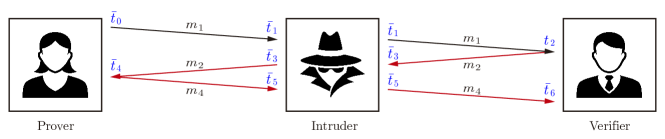
$$\{\emptyset{\mid}\{\emptyset\}{\mid}0.0\}\rightarrow_{p,0,1,{\textit{N}ew}} \{(p,0,1):{+}(m_{1}@t_{1})\cdots~{}|~{}\{\emptyset\}~{}|~{}{\color[rgb]{0,0,1}\bar{t}_{0}}=0.0\}\ \ m_{1}=\textit{commit}(n(p,f_{1}),s(p,f_{2}))$$

$$\rightarrow_{i,0,1,{\textit{N}ew}} \left\{\begin{array}[]{@{}l@{\ }}(p,0,1):{+}(m_{1}@t_{1})\cdots\\ (i.F,0,1):{-}(X@t^{\prime}_{1})\cdot{+}(X@t^{\prime}_{2})\end{array}\right|\{\emptyset\}~{}|~{}{\color[rgb]{0,0,1}\bar{t}_{0}}\}$$

$$\rightarrow_{p,0,1,+(m_{1})} \left\{\begin{array}[]{@{}l@{\ }}(p,0,2):{-}(N_{V}@t_{2})\ \cdots\\ (i.F,0,1):{-}(X@t^{\prime}_{1})\cdot{+}(X@t^{\prime}_{2})\end{array}\right|\{(m_{1}@(p,0):{\color[rgb]{0,0,1}\bar{t}_{0}}\to\emptyset)\}~{}|~{}{\color[rgb]{0,0,1}\bar{t}_{0}}\}$$

$$\rightarrow_{\textit{T}ime} \left\{\begin{array}[]{@{}l@{\ }}(p,0,2):{-}(N_{V}@t_{2})\ \cdots\\ (i.F,0,1):{-}(X@t^{\prime}_{1})\cdot{+}(X@t^{\prime}_{2})\end{array}\right|\{(m_{1}@(p,0):{\color[rgb]{0,0,1}\bar{t}_{0}}\to\emptyset)\}~{}|~{}{\color[rgb]{0,0,1}\bar{t}_{1}}=1.0\}$$

$$\rightarrow_{i,0,1,-(m_{1})} \left\{\begin{array}[]{@{}l@{\ }}(p,0,2):{-}(N_{V}@t_{2})\ \cdots\\ (i.F,0,2):{+}(m_{1}@t^{\prime}_{2})\end{array}\right|\{(m_{1}@(p,0):{\color[rgb]{0,0,1}\bar{t}_{0}}\to(i.F,0):{\color[rgb]{0,0,1}\bar{t}_{1}})\}~{}|~{}{\color[rgb]{0,0,1}\bar{t}_{1}}\}$$

$$\rightarrow_{i,0,3,+(m_{1})} \left\{\begin{array}[]{@{}l@{\ }}(p,0,2):{-}(N_{V}@t_{2})\ \cdots\\ (i.F,0,2):\mathit{nilP}\end{array}\right|\left\{\begin{array}[]{@{}l@{}}(m_{1}@(i.F,0):{\color[rgb]{0,0,1}\bar{t}_{1}}\to\emptyset\end{array}\right\}~{}|~{}{\color[rgb]{0,0,1}\bar{t}_{1}}\}$$

$$\rightarrow_{v,0,1,{\textit{N}ew}} \left\{\begin{array}[]{@{}l@{\ }}(p,0,2):{-}(N_{V}@t_{2})\ \cdots\\ (v,0,1):{-}(\textit{Commit}@t^{\prime\prime}_{1})\cdots\end{array}\right|\left\{\begin{array}[]{@{}l@{}}(m_{1}@(i.F,0):{\color[rgb]{0,0,1}\bar{t}_{1}}\to\emptyset)\end{array}\right\}~{}|~{}{\color[rgb]{0,0,1}\bar{t}_{1}}\}$$

$$\rightarrow_{\textit{T}ime} \left\{\begin{array}[]{@{}l@{\ }}(p,0,2):{-}(N_{V}@t_{2})\ \cdots\\ (v,0,1):{-}(\textit{Commit}@t^{\prime\prime}_{1})\cdots\end{array}\right|\left\{\begin{array}[]{@{}l@{}}(m_{1}@(i.F,0):{\color[rgb]{0,0,1}\bar{t}_{1}}\to\emptyset)\end{array}\right\}~{}|~{}{\color[rgb]{0,0,1}\bar{t}_{2}}=2.0\}$$

$$\rightarrow_{v,0,1,-(m_{1})} \left\{\begin{array}[]{@{}l@{\ }}(p,0,2):{-}(N_{V}@t_{2})\ \cdots\\ (v,0,2):{+}(m_{2}@t^{\prime\prime}_{2})\cdots\end{array}\right|\left\{\begin{array}[]{@{}l@{}}(m_{1}@(i.F,0):{\color[rgb]{0,0,1}\bar{t}_{1}}\to(v,0):{\color[rgb]{0,0,1}\bar{t}_{2}})\end{array}\right\}~{}|~{}{\color[rgb]{0,0,1}\bar{t}_{2}}\}\ \ m_{2}=n(v,f_{3})$$

$$\rightarrow_{v,0,2,+(m_{2})} \left\{\begin{array}[]{@{}l@{\ }}(p,0,2):{-}(N_{V}@t_{2})\ \cdots\\ (v,0,3):{-}(m_{3}@t^{\prime\prime}_{3})\cdots\end{array}\right|\left\{\begin{array}[]{@{}l@{}}(m_{2}@(v,0):{\color[rgb]{0,0,1}\bar{t}_{2}}\to\emptyset)\end{array}\right\}~{}|~{}{\color[rgb]{0,0,1}\bar{t}_{2}}\}\ \ m_{3}=(m_{2}\oplus N_{P})$$

$$\rightarrow_{i,1,1,{\textit{N}ew}} \left\{\begin{array}[]{@{}l@{\ }}(p,0,2):{-}(N_{V}@t_{2})\ \cdots\\ (v,0,3):{-}(m_{3}@t^{\prime\prime}_{3})\cdots\\ (i.F,1,1):{-}(X^{\prime}@t^{\prime\prime\prime}_{1})\cdot{+}(X^{\prime}@t^{\prime\prime\prime}_{2})\end{array}\right|\left\{\begin{array}[]{@{}l@{}}(m_{2}@(v,0):{\color[rgb]{0,0,1}\bar{t}_{2}}\to\emptyset)\end{array}\right\}~{}|~{}{\color[rgb]{0,0,1}\bar{t}_{2}}\}$$

$$\rightarrow_{\textit{T}ime} \left\{\begin{array}[]{@{}l@{\ }}(p,0,2):{-}(N_{V}@t_{2})\ \cdots\\ (v,0,3):{-}(m_{3}@t^{\prime\prime}_{3})\cdots\\ (i.F,1,1):{-}(X^{\prime}@t^{\prime\prime\prime}_{1})\cdot{+}(X^{\prime}@t^{\prime\prime\prime}_{2})\end{array}\right|\left\{\begin{array}[]{@{}l@{}}(m_{2}@(v,0):{\color[rgb]{0,0,1}\bar{t}_{2}}\to\emptyset)\end{array}\right\}~{}|~{}{\color[rgb]{0,0,1}\bar{t}_{3}}=3.0\}$$

$$\rightarrow_{i,1,1,-(m_{2})} \left\{\begin{array}[]{@{}l@{\ }}(p,0,2):{-}(N_{V}@t_{2})\ \cdots\\ (v,0,3):{-}(m_{3}@t^{\prime\prime}_{3})\cdots\\ (i.F,1,2):{+}(m_{2}@t^{\prime\prime\prime}_{2})\end{array}\right|\left\{\begin{array}[]{@{}l@{}}(m_{2}@(v,0):{\color[rgb]{0,0,1}\bar{t}_{2}}\to(i.F,1):{\color[rgb]{0,0,1}\bar{t}_{3}})\end{array}\right\}~{}|~{}{\color[rgb]{0,0,1}\bar{t}_{3}}\}$$

$$\rightarrow_{i,1,2,+(m_{2})} \left\{\begin{array}[]{@{}l@{\ }}(p,0,2):{-}(N_{V}@t_{2})\ \cdots\\ (v,0,3):{-}(m_{3}@t^{\prime\prime}_{3})\cdots\\ (i.F,1,2):\mathit{nilP}\end{array}\right|\left\{\begin{array}[]{@{}l@{}}(m_{2}@(i.F,1):{\color[rgb]{0,0,1}\bar{t}_{3}}\to\emptyset)\end{array}\right\}~{}|~{}{\color[rgb]{0,0,1}\bar{t}_{3}}\}$$

$$\rightarrow_{Time} \left\{\begin{array}[]{@{}l@{\ }}(p,0,2):{-}(N_{V}@t_{2})\ \cdots\\ (v,0,3):{-}(m_{3}@t^{\prime\prime}_{3})\cdots\end{array}\right|\left\{\begin{array}[]{@{}l@{}}(m_{2}@(i.F,1):{\color[rgb]{0,0,1}\bar{t}_{3}}\to\emptyset)\end{array}\right\}~{}|~{}{\color[rgb]{0,0,1}\bar{t}_{4}}=4.0\}$$

$$\rightarrow_{p,0,2,-(m_{2})} \left\{\begin{array}[]{@{}l@{\ }}(p,0,3):{+}(m_{4}@t_{3})\ \cdots\\ (v,0,3):{-}(m_{3}@t^{\prime\prime}_{3})\cdots\end{array}\right|\left\{\begin{array}[]{@{}l@{}}(m_{2}@(i.F,1):{\color[rgb]{0,0,1}\bar{t}_{3}}\to(p,0):{\color[rgb]{0,0,1}\bar{t}_{4}})\end{array}\right\}~{}|~{}{\color[rgb]{0,0,1}\bar{t}_{4}}\}\ \ m_{4}=(m_{2}\oplus n(p,f_{1}))$$

$$\rightarrow_{p,0,3,+(m_{4})} \left\{\begin{array}[]{@{}l@{\ }}(p,0,4):{+}(m_{5}@t_{4})\ \cdots\\ (v,0,3):{-}(m_{3}@t^{\prime\prime}_{3})\cdots\end{array}\right|\left\{\begin{array}[]{@{}l@{}}(m_{4}@(p,0):{\color[rgb]{0,0,1}\bar{t}_{4}}\to\emptyset)\end{array}\right\}~{}|~{}{\color[rgb]{0,0,1}\bar{t}_{4}}\}\ \ m_{5}=s(p,f_{2})$$

$$\rightarrow_{i,2,1,{\textit{N}ew}} \left\{\begin{array}[]{@{}l@{\ }}(v,0,3):{-}(m_{3}@t^{\prime\prime}_{3})\cdots\\ (i.F,2,1):{-}(X^{\prime\prime}@t^{\prime\prime\prime\prime}_{1})\cdot{+}(X^{\prime\prime}@t^{\prime\prime\prime\prime}_{2})\end{array}\right|\left\{\begin{array}[]{@{}l@{}}(m_{4}@(p,0):{\color[rgb]{0,0,1}\bar{t}_{4}}\to\emptyset)\end{array}\right\}~{}|~{}{\color[rgb]{0,0,1}\bar{t}_{4}}\}$$

$$\rightarrow_{\textit{T}ime} \left\{\begin{array}[]{@{}l@{\ }}(v,0,3):{-}(m_{3}@t^{\prime\prime}_{3})\cdots\\ (i.F,2,1):{-}(X^{\prime\prime}@t^{\prime\prime\prime\prime}_{1})\cdot{+}(X^{\prime\prime}@t^{\prime\prime\prime\prime}_{2})\end{array}\right|\left\{\begin{array}[]{@{}l@{}}(m_{4}@(p,0):{\color[rgb]{0,0,1}\bar{t}_{4}}\to\emptyset)\end{array}\right\}~{}|~{}{\color[rgb]{0,0,1}\bar{t}_{5}}=5.0\}$$

$$\rightarrow_{i,3,1,-(m_{4})} \left\{\begin{array}[]{@{}l@{\ }}(v,0,3):{-}(m_{3}@t^{\prime\prime}_{3})\cdots\\ (i.F,2,1):{+}(m_{4}@t^{\prime\prime\prime\prime}_{2})\end{array}\right|\left\{\begin{array}[]{@{}l@{}}(m_{4}@(p,0):{\color[rgb]{0,0,1}\bar{t}_{4}}\to(i.F,2):{\color[rgb]{0,0,1}\bar{t}_{5}})\end{array}\right\}~{}|~{}{\color[rgb]{0,0,1}\bar{t}_{5}}\}$$

$$\rightarrow_{i,3,2,+(m_{4})} \left\{\begin{array}[]{@{}l@{\ }}(v,0,3):{-}(m_{3}@t^{\prime\prime}_{3})\cdots\\ (i.F,2,1):\ nil\end{array}\right|\left\{\begin{array}[]{@{}l@{}}(m_{4}@(i.F,2):{\color[rgb]{0,0,1}\bar{t}_{5}}\to\emptyset)\end{array}\right\}~{}|~{}{\color[rgb]{0,0,1}\bar{t}_{5}}\}$$

$$\rightarrow_{\textit{T}ime} \left\{\begin{array}[]{@{}l@{\ }}(v,0,3):{-}(m_{3}@t^{\prime\prime}_{3})\cdots\end{array}\right|\left\{\begin{array}[]{@{}l@{}}(m_{4}@(i.F,2):{\color[rgb]{0,0,1}\bar{t}_{5}}\to\emptyset)\end{array}\right\}~{}|~{}{\color[rgb]{0,0,1}\bar{t}_{6}}=6.0\}$$

$$\rightarrow_{v,0,3,-(m_{4})} \left\{\begin{array}[]{@{}l@{\ }}(v,0,4):{-}(S_{P}@t_{4})\cdots\end{array}\right|\left\{\begin{array}[]{@{}l@{}}(m_{4}@(i.F,2):{\color[rgb]{0,0,1}\bar{t}_{5}}\to(v,0):{\color[rgb]{0,0,1}\bar{t}_{6}})\end{array}\right\}~{}|~{}{\color[rgb]{0,0,1}\bar{t}_{6}}\}$$

Figure 3: Brand and Chaum execution for a prover, an intruder, and a verifier

Example 4

Continuing Example 2, a possible run of the protocol is represented in Figure 3 for a prover $p$, an intruder $i$, and a verifier $v$. A simpler, graphical representation of the same run is included at the top of the figure. There, the neighborhood distance is $d=1.0$, the distance between the prover and the verifier is $d(p,v)=2.0$, but the distance between the prover and the intruder as well as the distance between the verifier and the intruder are $d(v,i)=d(p,i)=1.0$, i.e., the honest prover $p$ is outside $v$’s neighborhood, $d(v,p)>d$, where $d(v,p)=d(v,i)+d(p,i)$. Only the first part of the rapid message exchange sequence is represented and the forwarding action of the intruder is denoted by $i.F$.

The prover sends the commitment $m_{1}=\textit{commit}(n(p,f_{1}),s(p,f_{2}))$ at instant $\bar{t}_{0}=0.0$ and is received by the intruder at instant $\bar{t}_{1}=1.0$. The intruder forwards $m_{1}$ at instant $\bar{t}_{1}$ and is received by the verifier at instant $\bar{t}_{2}=2.0$. Then, the verifier sends $m_{2}=n(v,f_{3})$ at instant $\bar{t}_{2}$, which is received by the intruder at instant $\bar{t}_{3}=3.0$. The intruder forwards $m_{2}$ at instant $\bar{t}_{3}$, which is received by the prover at instant $\bar{t}_{4}=4.0$. Then, the prover sends $m_{4}=(m_{2}\oplus n(p,f_{1}))$ at instant $\bar{t}_{4}$ and is received by the intruder at instant $\bar{t}_{5}=5.0$. Finally, the intruder forwards $m_{4}$ at instant $\bar{t}_{5}$ and is received by the verifier at instant $\bar{t}_{6}=6.0$. Thus, the verifier sent $m_{2}$ at time $\bar{t}_{2}=2.0$ and received $m_{4}$ at time $\bar{t}_{6}=6.0$. But the protocol cannot complete the run, since $\bar{t}_{6}-\bar{t}_{2}=4.0<2*d=2.0$ is unsatisfiable.

Our time protocol semantics can already be implemented straightforwardly as a simulation tool. For instance, [18] describes distance bounding protocols using an authentication logic, which describes the evolution of the protocol, [23] provides a strand-based framework for distance bounding protocols based on simulation with time constraints, and [8] defines distance bounding protocol using some applied-pi calculus. Note, however, that, since the number of metric space configurations is infinite, model checking a protocol for a concrete configuration with a simulation tool is very limited, since it cannot prove the absence of an attack for all configurations. For this reason, we follow a symbolic approach that can explore all relevant configurations.

In the following section, we provide a sound and complete protocol transformation from our timed process algebra to the untimed process algebra of the Maude-NPA tool. In order to do this, we make use of an approach introduced by Nigam et al. [23] in which properties of time, which can include both those following from physics and those checked by principals, are represented by linear constraints on the reals. As a path is built, an SMT solver can be used to check that the constraints are satisfiable, as is done in [24].

4 Timed Process Algebra into Untimed Process Algebra with Time Variables and Timing Constraints

In this section, we consider a more general constraint satisfiability approach, where all possible (not only some) runs are symbolically analyzed. This provides both a trace-based insecure statement, i.e., a run leading to an insecure secrecy or authentication property is discovered given enough resources, and an unsatisfiability-based secure statement, i.e., there is no run leading to an insecure secrecy or authentication property due to time constraint unsatisfiability.

Example 5

Consider again the run of the Brands-Chaum protocol given in Figure 3. All the terms of sort $\mathsf{Real}$, written in blue color, are indeed variables that get an assignment during the run based on the distance function. Then, it is possible to obtain a symbolic trace from the run of Figure 3, where the following time constraints are accumulated:

• $\bar{t}_{1}=\bar{t}_{0}+d((p,0),(i.F,0))$, $d((p,0),(i.F,0))\geq 0$

• $\bar{t}_{2}=\bar{t}_{1}+d((v,0),(i.F,0))$, $d((v,0),(i.F,0))\geq 0$

• $\bar{t}_{3}=\bar{t}_{2}+d((v,0),(i.F,1))$, $d((v,0),(i.F,1))\geq 0$

• $\bar{t}_{4}=\bar{t}_{3}+d((p,0),(i.F,1))$, $d((p,0),(i.F,1))\geq 0$

• $\bar{t}_{5}=\bar{t}_{4}+d((p,0),(i.F,2))$, $d((p,0),(i.F,2))\geq 0$

• $\bar{t}_{6}=\bar{t}_{5}+d((v,0),(i.F,2))$, $d((v,0),(i.F,2))\geq 0$

Note that these constraints are unsatisfiable when combined with (i) the assumption $d>0$, (ii) the verifier check $\bar{t}_{6}-\bar{t}_{2}\leq 2*d$, (iii) the assumption that the honest prover is outside the verifier’s neighborhood, $d((p,0),\allowbreak(v,0))>d$, (iv) the triangular inequality from the metric space, $d((p,0),(v,0))\leq d((p,0),\allowbreak(i.F,0))+d(\allowbreak(i.F,0),(v,0))$, and (v) the assumption that there is only one intruder $d((i.F,0),\allowbreak(i.F,1))=0$ and $d((i.F,0),\allowbreak(i.F,2))=0$.

As explained previously in the remark, there are some implicit conditions based on the mte function to calculate the time increment to the closest destination of a message. However, the mte function disappears in the untimed process algebra and those implicit conditions are incorporated into the symbolic run. In the following, we define a transformation of the timed process algebra by (i) removing the global clock; (ii) adding the time data into untimed messages of a process algebra without time (as done in [23]); and (iii) adding linear arithmetic conditions over the reals for the time constraints (as is done in [24]). The soundness and completeness proof of the transformation is included in the additional supporting material at the end of the paper.

Since all the relevant time information is actually stored in messages of the form $M\ @\ ({A:t}\to(B_{1}:t_{1}\cdots B_{n}:t_{n}))$ and controlled by the transition rules (TPA++),(TPA+), and (TPA-), the mapping tpa2pa of Definition 1 below transforms each message $M@t$ of a timed process into a message $M\ @\ ({A:{\textit{t}}_{?}}\to{\textit{A}S}_{?})$ of an untimed process. That is, we use a timed choice variable ${\textit{t}}_{?}$ for the sending time and a variable ${\textit{A}S}_{?}$ for the reception information $(B_{1}:t^{\prime}_{1}\cdots B_{n}:t^{\prime}_{n})$ associated to the sent message. Since choice variables are replaced by specific values, both ${\textit{t}}_{?}$ and ${\textit{A}S}_{?}$ will be replaced by the appropriate values that make the execution and all its time constraints possible. Note that these two choice variables will be replaced by logical variables during the symbolic execution.

Definition 1 (Adding Time Variables and Time Constraints to Untimed Processes)

The mapping tpa2pa from timed processes into untimed processes and its auxiliary mapping tpa2pa​* are defined as follows:

$$\textit{tpa2pa}(\emptyset)=\mathit{\emptyset}$$

$$\textit{tpa2pa}((\mathit{ro}{,}i{,}j)\,P\ \&\ \mathit{PS})=(\textit{ro}{,}i{,}j)\,\textit{tpa2pa\!*}(P{,}\textit{ro}{,}i)\ \&\ \textit{tpa2pa}(\mathit{PS})$$

$$\textit{tpa2pa\!*}(\mathit{nilP},\textit{ro},i)=\mathit{nilP}$$

$$\textit{tpa2pa\!*}(\ +(M@t)\ .\ P,\textit{ro},i)=+(M@((\textit{ro},i):{\textit{t}}_{?}\to{\textit{A}S}_{?}))\ .\ \textit{tpa2pa\!*}(P\gamma,\textit{ro},i)$$

$$\hskip 14.22636pt\mbox{where }\gamma=\{t\mapsto{\textit{t}}_{?}\}$$

$$\textit{tpa2pa\!*}(\ -(M@t)\ .\ P,\textit{ro},i)=$$

$$\hskip 5.69054pt-(M@((\textit{ro}^{\prime},i^{\prime}):t^{\prime}\to((\textit{ro},i):t)\uplus AS))\ .\$$

$$\hskip 5.69054pt\textit{ if }t=t^{\prime}+d((\textit{ro},i),(\textit{ro}^{\prime},i^{\prime}))\wedge d((\textit{ro},i),(\textit{ro}^{\prime},i^{\prime}))\geq 0\textit{ then }\textit{tpa2pa\!*}(P,\textit{ro},i)\textit{ else }\mathit{nilP}$$

$$\textit{tpa2pa\!*}(\textit{ (if }C\textit{ then }P\textit{ else }Q)\ .\ R{,}\textit{ro}{,}i{,}x{,}y)$$

$$\hskip 5.69054pt=\textit{ (if }C\textit{ then }\textit{tpa2pa\!*}(P{,}\textit{ro}{,}i{,}x{,}y)\textit{ else }\textit{tpa2pa\!*}(Q{,}\textit{ro}{,}i{,}x{,}y))\ .\ \textit{tpa2pa\!*}(R{,}\textit{ro}{,}i{,}x{,}y)$$

$$\textit{tpa2pa\!*}(\ (P\ ?\ Q)\ .\ R{,}\textit{ro}{,}i{,}x{,}y)$$

$$\hskip 5.69054pt=\ (\textit{tpa2pa\!*}(P{,}\textit{ro}{,}i{,}x{,}y)\ ?\ \textit{tpa2pa\!*}(Q{,}\textit{ro}{,}i{,}x{,}y))\ .\ \textit{tpa2pa\!*}(R{,}\textit{ro}{,}i{,}x{,}y)$$

where ${\textit{t}}_{?}$ and ${\textit{A}S}_{?}$ are choice variables different for each one of the sending actions, $\textit{ro}^{\prime},i^{\prime},t^{\prime},d,AS$ are pattern variables different for each one of the receiving actions, $P$, $Q$, and $R$ are processes, $M$ is a message, and $C$ is a constraint.

Example 6

The timed processes of Example 2 are transformed into the following untimed processes. We remove the “else $\mathit{nilP}$” branches for clarity.

$$(\mathit{Verifier}):\ {-}(\textit{Commit}\ @\ A_{1}:t^{\prime}_{1}\to{\textit{V}}_{?}:t_{1}\uplus AS_{1})\ \cdot$$

$$\textit{if}\ t_{1}=t^{\prime}_{1}+d(A_{1},{\textit{V}}_{?})\wedge d(A_{1},{\textit{V}}_{?})\geq 0\textit{ then}$$

$${+}(n({\textit{V}}_{?},f_{1})\ @\ {\textit{V}}_{?}:{\textit{t}_{2}}_{?}\to{\textit{A}S_{2}}_{?})\ \cdot$$

$${-}((n({\textit{V}}_{?},f_{1})\oplus N_{P})\ @\ A_{3}:t^{\prime}_{3}\to{\textit{V}}_{?}:t_{3}\uplus AS_{3})\ \cdot$$

$$\textit{if}\ t_{3}=t^{\prime}_{3}+d(A_{3},{\textit{V}}_{?})\wedge d(A_{3},{\textit{V}}_{?})\geq 0\textit{ then}$$

$$\textit{if}\ t_{3}\dot{-}{\textit{t}_{2}}_{?}\leq 2*d\textit{ then}$$

$${-}(S_{P}\ @\ A_{4}:t^{\prime}_{4}\to{\textit{V}}_{?}:t_{4}\uplus AS_{4})\ \cdot$$

$$\textit{if}\ t_{4}=t^{\prime}_{4}+d(A_{4},{\textit{V}}_{?})\wedge d(A_{4},{\textit{V}}_{?})\geq 0\textit{ then}$$

$$\textit{if}\ \textit{open}(N_{P},S_{P},\textit{Commit})\textit{ then}$$

$${-}(\textit{sign}(P,n({\textit{V}}_{?},f_{1});N_{P}\oplus n({\textit{V}}_{?},f_{1}))\ @\ A_{5}:t^{\prime}_{5}\to{\textit{V}}_{?}:t_{5}\uplus AS_{5})$$

$$\textit{if}\ t_{5}=t^{\prime}_{5}+d(A_{5},{\textit{V}}_{?})\wedge d(A_{5},{\textit{V}}_{?})\geq 0$$

$$(\mathit{Prover}):\ {+}(\textit{commit}(n({\textit{P}}_{?},f_{1}),s({\textit{P}}_{?},f_{2}))@{\textit{P}}_{?}:{\textit{t}_{1}}_{?}\to{\textit{A}S_{1}}_{?})\ \cdot$$

$${-}(V;N_{V}@\ A_{2}:t^{\prime}_{2}\to{\textit{V}}_{?}:t_{2}\uplus AS_{2})\ \cdot$$

$$\textit{if}\ t_{2}=t^{\prime}_{2}+d(A_{2},{\textit{P}}_{?})\wedge d(A_{2},{\textit{P}}_{?})\geq 0\textit{ then}$$

$${+}((N_{V}\oplus n({\textit{P}}_{?},f_{1}))@{\textit{P}}_{?}:{\textit{t}_{3}}_{?}\to{\textit{A}S_{3}}_{?})\ \cdot$$

$${+}(s({\textit{P}}_{?},f_{2})@{\textit{P}}_{?}:{\textit{t}_{4}}_{?}\to{\textit{A}S_{4}}_{?})\ \cdot$$

$${+}(\textit{sign}({\textit{P}}_{?},N_{V};n({\textit{P}}_{?},f_{2})\oplus N_{V})@{\textit{P}}_{?}:{\textit{t}_{5}}_{?}\to{\textit{A}S_{5}}_{?}))$$

Example 7

The timed processes of Example 3 for the intruder are transformed into the following untimed processes. Note that we use the intruder identifier $I$ associated to each role instead of a choice variable ${\textit{I}}_{?}$.

$$(\mathit{I.Conc}):\ {-}(X@\ A_{1}:t_{1}\to I:t^{\prime}_{1}\uplus AS_{1})\ \cdot$$

$$\textit{if}\ t^{\prime}_{1}=t_{1}+d(A_{1},I)\wedge d(A_{1},I)\geq 0\textit{ then}$$

$${-}(Y@\ A_{2}:t_{2}\to I:t^{\prime}_{2}\uplus AS_{2})\ \cdot$$

$$\textit{if}\ t^{\prime}_{2}=t_{2}+d(A_{2},I)\wedge d(A_{2},I)\geq 0\textit{ then}$$

$${+}(X;Y@I:{\textit{t}_{3}}_{?}\to{\textit{A}S}_{?})$$

$$(\mathit{I.Deconc}):\ {-}(X;Y@\ A_{1}:t_{1}\to I:t^{\prime}_{1}\uplus AS_{1})\ \cdot$$

$$\textit{if}\ t^{\prime}_{1}=t_{1}+d(A_{1},I)\wedge d(A_{1},I)\geq 0\textit{ then}$$

$${+}(X@I:{\textit{t}_{2}}_{?}\to{\textit{A}S}_{?})$$

$$(\mathit{I.Forward}):\ {-}(X@\ A_{1}:t_{1}\to I:t^{\prime}_{1}\uplus AS_{1})\ \cdot$$

$$\textit{if}\ t^{\prime}_{1}=t_{1}+d(A_{1},I)\wedge d(A_{1},I)\geq 0\textit{ then}$$

$${+}(X@I:{\textit{t}_{2}}_{?}\to{\textit{A}S}_{?})$$

Once a timed process is transformed into an untimed process with time variables and time constraints using the notation of Maude-NPA, we rely on both a soundness and completeness proof from the Maude-NPA process notation into Maude-NPA forward rewriting semantics and on a soundness and completeness proof from Maude-NPA forward rewriting semantics into Maude-NPA backwards symbolic semantics, see [30, 29]. Since the Maude-NPA backwards symbolic semantics already considers constraints in a very general sense [12], we only need to perform the additional satisfiability check for linear arithmetic over the reals.

5 Timed Process Algebra into Strands in Maude-NPA

This section is provided to help in understanding the experimental output. Although Maude-NPA accepts protocol specifications in either the process algebra language or the strand space language, it still gives outputs only in the strand space notation. Thus, in order to make our experimental output easier to understand, we describe the translation from timed process into strands with time variables and time constraints. This translation is also sound and complete, as it imitates the transformation of Section 4 and the transformation of [30, 29].

Strands [28] are used in Maude-NPA to represent both the actions of honest principals (with a strand specified for each protocol role) and those of an intruder (with a strand for each action an intruder is able to perform on messages). In Maude-NPA, strands evolve over time. The symbol $|$ is used to divide past and future. That is, given a strand $[\ \textit{msg}_{1}^{\pm},\ \ldots,\ \textit{msg}_{i}^{\pm}\ |\allowbreak\ \textit{msg}_{i+1}^{\pm},\ \ldots,\ \textit{msg}_{k}^{\pm}\ ]$, messages $\textit{msg}_{1}^{\pm},\linebreak[2]\ldots,\textit{msg}_{i}^{\pm}$ are the past messages, and messages $\textit{msg}_{i+1}^{\pm},\ldots,\textit{msg}_{k}^{\pm}$ are the future messages ($\textit{msg}_{i+1}^{\pm}$ is the immediate future message). Constraints can be also inserted into strands. A strand $[\textit{msg}_{1}^{\pm},\linebreak[2]\ldots,\linebreak[2]\textit{msg}_{k}^{\pm}]$ is shorthand for $[nil~{}|~{}\textit{msg}_{1}^{\pm},\linebreak[2]\ldots,\linebreak[2]\textit{msg}_{k}^{\pm},nil]$. An initial state is a state where the bar is at the beginning for all strands in the state, and the network has no possible intruder fact of the form $\textit{m}{\ \in\ }{\mathcal{I}}$. A final state is a state where the bar is at the end for all strands in the state and there is no negative intruder fact of the form $\textit{m}{\ \notin\ }{\mathcal{I}}$.

In the following example, we illustrate how the timed process algebra can be transformed into strands specifications of Maude-NPA.

Example 8

The timed processes of Example 2 are transformed into the following strand specification.

$$(\mathit{Verifier}):\ [ {-}(\textit{Commit}\ @\ A_{1}:t^{\prime}_{1}\to V:t_{1}\uplus AS_{1}),$$

$$(t_{1}=t^{\prime}_{1}+d(A_{1},V)\wedge d(A_{1},V)\geq 0),$$

$${+}(n(V,f_{1})\ @\ V:t_{2}\to AS_{2}),$$

$${-}((n(V,f_{1})\oplus N_{P})\ @\ A_{3}:t^{\prime}_{3}\to V:t_{3}\uplus AS_{3}),$$

$$(t_{3}=t^{\prime}_{3}+d(A_{3},V)\wedge d(A_{3},V)\geq 0),$$

$$(t_{3}\dot{-}t_{2}\leq 2*d),$$

$${-}(S_{P}\ @\ A_{4}:t^{\prime}_{4}\to V:t_{4}\uplus AS_{4}),$$

$$(t_{4}=t^{\prime}_{4}+d(A_{4},V)\wedge d(A_{4},V)\geq 0),$$

$$\textit{open}(N_{P},S_{P},\textit{Commit}),$$

$${-}(\textit{sign}(P,n(V,f_{1});N_{P}\oplus n(V,f_{1}))@\ A_{5}:t^{\prime}_{5}\to V:t_{5}\uplus AS_{5}),$$

$$(t_{5}=t^{\prime}_{5}+d(A_{5},V)\wedge d(A_{5},V)\geq 0)]$$

$$(\mathit{Prover}):\ [ {+}(\textit{commit}(n(P,f_{1}),s(P,f_{2}))@P:t_{1}\to AS_{1}),$$

$${-}(N_{V}@\ A_{2}:t^{\prime}_{2}\to V:t_{2}\uplus AS_{2}),$$

$$(t_{2}=t^{\prime}_{2}+d(A_{2},P)\wedge d(A_{2},P)\geq 0),$$

$${+}((N_{V}\oplus n(P,f_{1}))@P:t_{3}\to AS_{3}),$$

$${+}(s(P,f_{2})@P:t_{4}\to AS_{4}),$$

$${+}(\textit{sign}(P,N_{V};n(P,f_{2})\oplus N_{V})@P:t_{5}\to AS_{5})]$$

We specify the desired security properties in terms of attack patterns including logical variables, which describe the insecure states that Maude-NPA is trying to prove unreachable. Specifically, the tool attempts to find a backwards narrowing sequence path from the attack pattern to an initial state until it can no longer form any backwards narrowing steps, at which point it terminates. If it has not found an initial state, the attack pattern is judged unreachable.

The following example shows how a classic mafia fraud attack for the Brands-Chaum protocol can be encoded in Maude-NPA’s strand notation.

Example 9

Following the strand specification of the Brands-Chaum protocol given in Example 8, the mafia attack of Example 1 is given as the following attack pattern. Note that Maude-NPA uses symbol === for equality on the reals, +=+ for addition on the reals, *=* for multiplication on the reals, and -=- for subtraction on the reals. Also, we consider one prover p, one verifier v, and one intruder i at fixed locations. Extra time constraints are included in an smt section, where a triangular inequality has been added. The mafia fraud attack is secure for Brands-Chaum and no initial state is found in the backwards search.

       eq ATTACK-STATE(1) ---  Mafia fraud
          = :: r :: --- Verifier
            [ nil, -(commit(n(p,r1),s(p,r2))  @ i : t1 -> v : t2),
                    ((t2 === t1 +=+ d(i,v)) and d(i,v) >= 0/1),
                    +(n(v,r)                  @ v : t2 -> i : t2’’),
                    -(n(v,r) * n(p,r1)        @ i : t3 -> v : t4),
                    (t3 >= t2 and (t4 === t3 +=+ d(i,v)) and d(i,v) >= 0/1),
                    ((t4 -=- t2) <= (2/1 *=* d)) | nil ] &
            :: r1,r2 :: --- Prover
            [ nil,  +(commit(n(p,r1),s(p,r2)) @ p : t1’ -> i : t1’’),
                    -(n(v,r) @ i : t2’’ -> p : t3’),
                    ((t3’ === t2’’ +=+ d(i,p)) and d(i,p) >= 0/1),
                    +(n(v,r) * n(p,r1)        @ p : t3’ -> i : t3’’) | nil ]
            || smt(d(v,p) > 0/1 and d(i,p) > 0/1 and d(i,v) > 0/1 and d(v,i) <= d and
                    (d(v,i) +=+ d(p,i)) >= d(v,p) and d(v,p) > d)
            || nil || nil || nil [nonexec] .

6 Experiments

As a feasibility study, we have encoded several distance bounding protocols in Maude-NPA. It was necessary to slightly alter the Maude-NPA tool by (i) including minor modifications to the state space reduction techniques to allow for timed messages; (ii) the introduction of the sort Real and its associated operations; and (iii) the connection of Maude-NPA to a Satisfiability Modulo Theories (SMT) solver (see [22] for details on SMT). The specifications, outputs, and the modified version of Maude-NPA are available at http://personales.upv.es/sanesro/indocrypt2020/.

Although the timed model allows an unbounded number of principals, the attack patterns used to specify insecure goal states allow us to limit the number of principals in a natural way. In this case we specified one verifier, one prover, and one attacker, but allowed an unbounded number of sessions.

Protocol	PreProc (sec)	Mafia	tm (sec)	Hijacking	tm (sec)
Brands and Chaum [3]	3.0	$\checkmark$	4.3	$\times$	11.4
Meadows et al ($n_{V}\oplus n_{P}$,$P$) [18]	3.7	$\checkmark$	1.3	$\checkmark$	22.5
Meadows et al ($n_{V}$,$n_{P}\oplus P$) [18]	3.5	$\checkmark$	1.1	$\times$	1.5
Hancke and Kuhn [13]	1.2	$\checkmark$	12.5	$\checkmark$	0.7
MAD [4]	5.1	$\checkmark$	110.5	$\times$	318.8
Swiss-Knife [14]	3.1	$\checkmark$	4.8	$\checkmark$	24.5
Munilla et al. [20]	1.7	$\checkmark$	107.1	$\checkmark$	4.5
CRCS [27]	3.0	$\checkmark$	450.1	$\times$	68.6
TREAD [1]	2.4	$\checkmark$	4.7	$\times$	4.2

Table 1: Experiments performed for different distance-bounding protocols

In Table 1 above we present the results for the different distance-bounding protocols that we have analyzed. Two attacks have been analyzed for each protocol: a mafia fraud attack (i.e., an attacker tries to convince the verifier that an honest prover is closer to him than he really is), and a distance hijacking attack (i.e., a dishonest prover located far away succeeds in convincing a verifier that they are actually close, and he may only exploit the presence of honest participants in the neighborhood to achieve his goal). Symbol $\checkmark$ means the property is satisfied and $\times$ means an attack was found. The columns labelled $tm(sec)$ give the times in seconds that it took for a search to complete. Finally the column labeled PreProc gives the time it takes Maude-NPA to perform some preprocessing on the specification that eliminates searches for some provably unreachable state. This only needs to be done once, after which the results can be used for any query, so it is displayed separately.

We note that, since our semantics is defined over arbitrary metric spaces, not just Euclidean space, it is also necessary to verify that an attack returned by the tool is realizable over Euclidean space. We note that the Mafia and hijacking attacks returned by Maude-NPA in these experiments are all realizable on a straight line, and hence are realizable over $n$-dimensional Euclidean space for any $n$. In general, this realizability check can be done via a final step in which the constraints with the Euclidean metric substituted for distance is checked via an SMT solver that supports checking quadratic constraints over the reals, such as Yices [31], Z3 [32], or Mathematica [15]. Although this feature is not yet implemented in Maude-NPA, we have begun experimenting with these solvers.

7 Conclusions

We have developed a timed model for protocol analysis based on timing constraints, and provided a prototype extension of Maude-NPA handling protocols with time by taking advantage of Maude’s support of SMT solvers, as was done by Nigam et al. in [24], and Maude-NPA’s support of constraint handling. We also performed some initial analyses to test the feasibility of the approach. This approach should be applicable to other tools that support constraint handling.

There are several ways this work can be extended. One is to extend the ability of the tool to reason about a larger numbers or principals, in particular an unbounded number of principals. This includes an unbounded number of attackers; since each attacker must have its own location, we cannot assume a single attacker as in Dolev-Yao. Our specification and query language, and its semantics, supports reasoning about an unbounded number of principals, so this is a question of developing means of telling when a principal or state is redundant and developing state space reduction techniques based on this.

Another important extension is to protocols that require the full Euclidean space model, in particular those in which location needs to be explicitly included in the constraints. This includes for example protocols used for localization. For this, we have begun experimenting with SMT solvers that support solving quadratic constraints over the reals.

Looking further afield, we consider adding different types of timing models. In the timing model used in this paper, time is synonymous with distance. But we may also be interested including other ways in which time is advanced, e.g. the amount of time a principal takes to perform internal processing tasks. In our model, the method in which timing is advanced is specified by the $mte$ function, which is in turn used to generate constraints on which messages can be ordered. Thus changing the way in which timing is advanced can be accomplished by modifying the $mte$ function. Thus, potential future research includes design of generic $mte$ functions together with rules on their instantiation that guarantee soundness and completeness

Finally, there is also no reason for us to limit ourselves to time and location. This approach should be applicable to other quantitative properties as well. For example, the inclusion of cost and utility would allow us to tackle new classes of problems not usually addressed by cryptographic protocol analysis tools, such as performance analyses (e.g., resistance against denial of service attacks), or even analysis of game-theoretic properties of protocols, thus opening up a whole new set of problems to explore.

Additional Supporting Material

In order to prove soundness and completeness of the transformation in Appendix 0.B, we first recall the untimed process algebra of Maude-NPA.

Appendix 0.A (Untimed) Process Algebra

Maude-NPA was originally defined [10, 11] using strands [28]. A process algebra that extends the strand space model to naturally specify protocols exhibiting choice points was given in [30, 29]. Here we give a high-level summary of the untimed process algebra syntax of Maude-NPA, see [16].

0.A.1 Syntax of the Protocol Process Algebra

In the protocol process algebra the behaviors of both honest principals and the intruder are represented by labeled processes. Therefore, a protocol is specified as a set of labeled processes. Each process performs a sequence of actions, namely, sending or receiving a message, and may perform deterministic or non-deterministic choices. The protocol process algebra’s syntax $\Sigma_{\mathit{PA}}$ is parameterized by a sort $\mathsf{Msg}$ of messages and a sort $\mathsf{Cond}$ for conditional expressions. It has the following syntax:

$$\mathit{ProcConf}~{} ::=\mathit{LProc}~{}|~{}\mathit{ProcConf}~{}\&~{}\mathit{ProcConf}~{}|~{}\emptyset$$

$$\mathit{LProc}~{} ::=(\mathit{Role},I,J)~{}\mathit{Proc}$$

$$\mathit{Proc}~{} ::=\mathit{nilP}~{}|~{}+\mathit{Msg}~{}|~{}-\mathit{Msg}~{}|~{}\mathit{Proc}\cdot\mathit{Proc}~{}|$$

$$~{}~{}~{}~{}~{}~{}~{}\mathit{Proc}~{}?~{}\mathit{Proc}~{}|~{}\textit{if}~{}\mathit{Cond}~{}\textit{then}~{}\mathit{Proc}~{}\textit{else}~{}\mathit{Proc}$$

• $\mathit{ProcConf}$ stands for a process configuration, that is, a set of labeled processes. The symbol & is used to denote set union for sets of labeled processes.

• $\mathit{LProc}$ stands for a labeled process, that is, a process $\mathit{Proc}$ with a label $(\mathit{Role},I,J)$. $\mathit{Role}$ refers to the role of the process in the protocol (e.g., initiator or responder). $I$ is a natural number denoting the identity of the process, which distinguishes different instances(sessions) of a process specification. $J$ indicates that the action at stage $J$ of the process specification will be the next one to be executed, that is, the first $J-1$ actions of the process for role $\mathit{Role}$ have already been executed. Note that we omit $I$ and $J$ in the protocol specification when both $I$ and $J$ are $0$.

• $\mathit{Proc}$ defines the actions that can be executed within a process. ${+\mathit{Msg}}$, and ${-\mathit{Msg}}$ respectively denote sending out or receiving a message $\mathit{Msg}$. We assume a single channel, through which all messages are sent or received by the intruder. “$\mathit{Proc}~{}\cdot~{}\mathit{Proc}$” denotes sequential composition of processes, where symbol _._ is associative and has the empty process $\mathit{nilP}$ as identity. “$\mathit{Proc}~{}?~{}\mathit{Proc}$” denotes an explicit nondeterministic choice, whereas “$\textit{if}~{}\mathit{Cond}~{}\textit{then}\allowbreak~{}\mathit{Proc}~{}\textit{else}~{}\mathit{Proc}$” denotes an explicit deterministic choice, whose continuation depends on the satisfaction of the constraint $\mathit{Cond}$. In [30, 29], either equalities ($=$) or disequalities ($\neq$) between message expressions were considered as constraints.

Let $PS,~{}QS$, and $RS$ be process configurations, and $P,~{}Q$, and $R$ be protocol processes. The protocol syntax satisfies the following structural axioms:

$$PS\,\&\,QS=QS\,\&\,PS$$

$$(PS\,\&\,QS)\,\&\,RS=PS\,\&\,(QS\,\&\,RS)$$

$$(P\,\cdot\,Q)\cdot\,R=P\,\cdot\,(Q\,\cdot\,R)$$

$$PS\ \&\ \emptyset=PS$$

$$P\,\cdot\,\mathit{nilP}=P$$

$$\mathit{nilP}\,\cdot\,P=P$$

The specification of the processes defining a protocol’s behavior may contain some variables denoting information that the principal executing the process does not yet know, or that will be different in different executions. In all protocol specifications we assume three disjoint kinds of variables:

• fresh variables: these are not really variables in the standard sense, but names for constant values in a data type $\mathsf{V_{fresh}}$ of unguessable values such as nonces. A fresh variable $f$ is always associated with a role $ro\in Role$ in the protocol. Throughout this paper we will denote this kind of variables as $f,f_{1},f_{2},\ldots$.

• choice variables: variables first appearing in a sent message $\mathit{+M}$, which can be substituted by any value arbitrarily chosen from a possibly infinite domain. A choice variable indicates an implicit non-deterministic choice. Given a protocol with choice variables, each possible substitution of these variables denotes a possible continuation of the protocol. We always denote choice variables by uppercase letters postfixed with the symbol “?” as a subscript, e.g., ${\textit{A}}_{?},{\textit{B}}_{?},\ldots$.

• pattern variables: variables first appearing in a received message $\mathit{-M}$. These variables will be instantiated when matching sent and received messages. Implicit deterministic choices are indicated by terms containing pattern variables, since failing to match a pattern term may lead to the rejection of a message. A pattern term plays the implicit role of a guard, so that, depending on the different ways of matching it, the protocol can have different continuations. This kind of variables will be written with uppercase letters, e.g., $A,B,N_{A},\ldots$.

Note that fresh variables are distinguished from other variables by having a specific sort $\mathsf{Fresh}$. Choice variables or pattern variables can never have sort $\mathsf{Fresh}$.

We consider only well-formed processes using the function $\mathit{wf}:\mathit{\mathit{Proc}}\rightarrow\mathit{Bool}$ defined in Figure 4. The definition of $\mathit{wf}$ uses an auxiliary function $\mathit{shVar}:\mathit{\mathit{Proc}}\rightarrow\mathit{VarSet}$ defined in Figure 5. Note that the well-formedness property implies that if a process begins with a deterministic choice action if T then Q else R, then all variables in $T$ must be instantiated, and thus only one branch may be taken. For this reason, it is undesirable to specify processes that begin with such an action. Furthermore, note that the well-formedness property avoids explicit choices where both possibilities are the $\mathit{nilP}$ process. That is, processes containing either (if T then nil else nil), or (nil ? nil), respectively.

$$\mathit{wf}(P\cdot+M)=\mathit{wf}(P)\hskip 7.74997pt\textit{if}~{}(\mathit{Vars}(M)\cap\mathit{Vars}(P))\subseteq\mathit{shVar}(P)$$

$$\mathit{wf}(P\cdot-M)=\mathit{wf}(P)\hskip 7.74997pt\textit{if}~{}(\mathit{Vars}(M)\cap\mathit{Vars}(P))\subseteq\mathit{shVar}(P)$$

$$\mathit{wf}(P\cdot(\textit{if}~{}~{}T~{}\textit{then}~{}Q~{}\textit{else}~{}R))=\mathit{wf}(P\cdot Q)\wedge\mathit{wf}(P\cdot R)$$

$$\hskip 7.74997pt\textit{if}\ P\neq\mathit{nilP}\ \textit{and }\ Q\neq\mathit{nilP}\ \textit{and }\mathit{Vars}(T)\subseteq\mathit{shVar}(P)$$

$$\mathit{wf}(P\cdot(Q~{}?~{}R))=\mathit{wf}(P\cdot Q)\wedge\mathit{wf}(P\cdot R)\hskip 7.74997pt\textit{ if }Q\neq\mathit{nilP}\ \textit{or}R\neq\mathit{nilP}$$

$$\mathit{wf}(P\cdot~{}\mathit{nilP})=\mathit{wf}(P)$$

$$\mathit{wf}(\mathit{nilP})=\textit{True}.$$

Figure 4: The well-formed function

$$\mathit{shVar}(+M~{}\cdot P)=\mathit{Vars}(M)\cup\mathit{shVar}(P)$$

$$\mathit{shVar}(-M~{}\cdot P)=\mathit{Vars}(M)\cup\mathit{shVar}(P)$$

$$\mathit{shVar}((\textit{if}~{}T~{}\textit{then}~{}P~{}\textit{else}~{}Q)~{}\cdot R)$$

$$~{}~{}~{}~{}~{}~{}=\mathit{Vars}(T)\cup(\mathit{shVar}(P)\cap\mathit{shVar}(Q))\cup\mathit{shVar}(R)$$

$$\mathit{shVar}((P~{}?~{}Q)~{}\cdot R)=(\mathit{shVar}(P)\cap\mathit{shVar}(Q))\cup\mathit{shVar}(R)$$

$$\mathit{shVar}(\mathit{nilP})=\emptyset$$

Figure 5: The shared variables function

0.A.2 Protocol Specification in Process Algebra

We define a protocol ${\mathcal{P}}$ in the protocol process algebra, written ${\mathcal{P}}_{\mathit{PA}}$, as a pair of the form ${\mathcal{P}}_{\mathit{PA}}=((\Sigma_{\mathit{{PA}_{\mathcal{P}}}},E_{\mathit{\textit{PA}_{\mathcal{P}}}}),P_{\mathit{PA}})$, where $(\Sigma_{\mathit{{PA}_{\mathcal{P}}}},E_{\mathit{\textit{PA}_{\mathcal{P}}}})$ is the equational theory specifying the equational properties of the cryptographic functions and the state structure, and $P_{\mathit{PA}}$ is a term denoting a well-formed process configuration representing the behavior of the honest principals as well as the capabilities of the attacker. That is, $P_{\mathit{PA}}=(\mathit{ro_{1}})P_{1}~{}\&~{}\ldots~{}\&~{}(\mathit{ro_{i}})P_{i}$, where each $ro_{k}$, $1\leq k\leq i$, is either the role of an honest principal or identifies one of the capabilities of the attacker. $P_{\mathit{PA}}$ cannot contain two processes with the same label, i.e., the behavior of each honest principal, and each attacker capability are represented by a unique process. $E_{\mathit{\textit{PA}_{\mathcal{P}}}}=E_{{\mathcal{P}}}\cup E_{\mathit{PA}}$ is a set of equations with $E_{{\mathcal{P}}}$ denoting the protocol’s cryptographic properties and $E_{\mathit{PA}}$ denoting the properties of process constructors. The set of equations $E_{{\mathcal{P}}}$ is user-definable and can vary for different protocols. Instead, the set of equations $E_{\mathit{PA}}$ is always the same for all protocols. $\Sigma_{\mathit{{PA}_{\mathcal{P}}}}=\Sigma_{\mathcal{P}}\cup\Sigma_{\mathit{PA}}$ is the signature defining the sorts and function symbols as follows:

• $\Sigma_{\mathcal{P}}$ is an order-sorted signature defining the sorts and function symbols for the messages that can be exchanged in protocol ${\mathcal{P}}$. However, independently of protocol ${\mathcal{P}}$, $\Sigma_{\mathcal{P}}$ must always have two sorts $\mathsf{Msg}$ and $\mathsf{Cond}$ as the top sorts in one of its connected components.

• $\Sigma_{\mathit{PA}}$ is an order-sorted signature defining the sorts and function symbols of the process algebra infrastructure. $\Sigma_{\mathit{PA}}$ corresponds exactly to the BNF definition of the protocol process algebra’s syntax in Section 0.A.1.

Therefore, the syntax $\Sigma_{\mathit{{PA}_{\mathcal{P}}}}$ of processes for ${\mathcal{P}}$ will be in the union signature $\Sigma_{\mathit{PA}}\cup\Sigma_{\mathcal{P}}$, consisting of the protocol-specific syntax $\Sigma_{\mathcal{P}}$, and the generic process syntax $\Sigma_{\mathit{PA}}$ through the shared sort $\mathsf{Msg}$.

0.A.3 Process Algebra Semantics

Given a protocol $\mathcal{P}$, a state of ${\mathcal{P}}$ consists of a set of (possibly partially executed) labeled processes, and a set of terms in the intruder knowledge $\{IK\}$. That is, a state is a term of the form n $\{LP_{1}\,\&\,\cdots\,\&\,LP_{n}~{}|~{}\{\textit{IK}\}\}$. Given a state $St$ of this form, we abuse notation and write $LP_{k}\in St$ if $LP_{k}$ is a labeled process in the set $LP_{1}\,\&\,\cdots\,\&\,LP_{n}$.

The intruder knowledge IK models the single channel through which all messages are sent and received. Messages are stored in the form $M{\ \in\ }{\mathcal{I}}$. We consider an active attacker who has complete control of the channel, i.e, can read, alter, redirect, and delete traffic as well as create its own messages by means of intruder processes. That is, the purpose of some $LP_{k}\in St$ is to perform message-manipulation actions for the intruder.

State changes are defined by a set $R_{\mathit{\textit{PA}_{\mathcal{P}}}}$ of rewrite rules, such that the rewrite theory $(\Sigma_{\mathit{{\textit{PA}_{\mathcal{P}}+State}}},E_{\mathit{\textit{PA}_{\mathcal{P}}}},R_{\mathit{\textit{PA}_{\mathcal{P}}}})$ characterizes the behavior of protocol ${\mathcal{P}}$, where $\Sigma_{\mathit{{\textit{PA}_{\mathcal{P}}+State}}}$ extends $\Sigma_{\mathit{{PA}_{\mathcal{P}}}}$ by adding state constructor symbols. We assume that a protocol’s execution begins with an empty state, i.e., a state with an empty set of labeled processes, and an empty network. That is, the initial state is always of the form $\{\emptyset~{}|~{}\{\emptyset\}\}$. Each transition rule in $R_{\mathit{\textit{PA}_{\mathcal{P}}}}$ is labeled with a tuple of the form $\mathit{(ro,i,j,a,n)}$, where:

• $\mathit{ro}$ is the role of the labeled process being executed in the transition.

• $i$ denotes the identifier of the labeled process being executed in the transition. Since there can be more than one process instance of the same role in a process state, $i$ is used to distinguish different instances, i.e., $ro$ and $i$ together uniquely identify a process in a state.

• $j$ denotes the process’ step number since its beginning.

• $a$ is a ground term identifying the action that is being performed in the transition. It has different possible values: “$+m$” or “$-m$” if the message $m$ was sent (and added to the network) or received, respectively; “$m$” if the message $m$ was sent but did not increase the network, “$?$” if the transition performs an explicit non-deterministic choice, or “$\mathit{T}$” if the transition performs an explicit deterministic choice.

• $n$ is a number that, if the action that is being executed is an explicit choice, indicates which branch has been chosen as the process continuation. In this case $n$ takes the value of either $1$ or $2$. If the transition does not perform any explicit choice, then $n=0$.

The set $R_{\mathit{\textit{PA}_{\mathcal{P}}}}$ of transition rules that define the execution of a state are given in [30, 29]. Note that in the transition rules $R_{\mathit{\textit{PA}_{\mathcal{P}}}}$ shown below, $PS$ denotes the rest of labeled processes of the state (which can be the empty set $\emptyset$).

• The action of sending a message is represented by the two transition rules below. Since we assume the intruder has complete control of the network, it can learn any message sent by other principals. Rule (PA++) denotes the case in which the sent message is added to the intruder knowledge. Note that this rule can only be applied if the intruder has not already learnt that message. Rule (PA+) denotes the case in which the intruder chooses not to learn the message, i.e., the intruder knowledge is not modified, and, thus, no condition needs to be checked. Since choice variables denote messages that are nondeterministically chosen, all (possibly infinitely many) admissible ground substitutions for the choice variables are possible behaviors.

  $$\{(ro,i,j)~{}(+M\cdot P)~{}\&~{}PS~{}|~{}\{IK\}\}$$

  $$\longrightarrow_{(ro,i,j,+M\sigma,0)}\{(ro,i,j+1)~{}P\sigma~{}\&~{}PS~{}|~{}\{M\sigma{\ \in\ }{\mathcal{I}},IK\}\}$$

  $$\textit{ if }(M\sigma{\ \in\ }{\mathcal{I}})\notin\textit{IK}$$

  $$\textit{where }\sigma\ \textit{is a ground substitution}\textit{ binding choice variables}\textit{ in}\ M$$ (PA++)

  $$\{(ro,i,j)~{}(+M\cdot P)~{}\&~{}PS~{}|~{}\{IK\}\}$$

  $$\longrightarrow_{(ro,i,j,M\sigma,0)}\{(ro,i,j+1)~{}P\sigma~{}\&~{}PS~{}|~{}\{IK\}\}$$

  $$\textit{where }\sigma\ \textit{is a ground substitution}\ \textit{binding choice variables}\textit{ in}\ M$$ (PA+)

• As shown in the rule below, a process can receive a message matching a pattern $M$ if there is a message $M^{\prime}$ in the intruder knowledge, i.e., a message previously sent either by some honest principal or by some intruder process, that matches the pattern message $M$. After receiving this message the process will continue with its variables instantiated by the matching substitution, which takes place modulo the equations $E_{\mathcal{P}}$. Note that the intruder can “delete” a message via choosing not to learn it (executing Rule PA+ instead of Rule PA++) or not to deliver it (failing to execute Rule PA-).

  $$\{(ro,i,j)~{}(-M\cdot P)~{}\&~{}PS\mid\{M^{\prime}{\ \in\ }{\mathcal{I}},IK\}\}$$

  $$\longrightarrow_{(ro,i,j,-M\sigma,0)}\{(ro,i,j+1)~{}P\sigma~{}\&~{}PS\mid\{M^{\prime}{\ \in\ }{\mathcal{I}},IK\}\}$$

  $$~{}\textit{if}~{}M^{\prime}=_{E_{{\mathcal{P}}}}M\sigma$$ (PA-)

• The two transition rules shown below define the operational semantics of explicit deterministic choices. That is, the operational semantics of an $\textit{if}~{}T~{}\textit{then}~{}P~{}\allowbreak\textit{else}~{}Q$ expression. More specifically, rule (PAif1) describes the then case, i.e., if the constraint $T$ is satisfied, the process will continue as $P$. Rule (PAif2) describes the else case, that is, if the constraint $T$ is not satisfied, the process will continue as $Q$. Note that, since we only consider well-formed processes, these transition rules will only be applied if $j\geq 1$. Note also that since $T$ has been fully substituted by the time the if-then-else is executed, the validity of $T$ can be easily checked.

  $$\{(ro,i,j)~{}((\textit{if}~{}T~{}\textit{then}~{}P~{}\textit{else}~{}Q)~{}\cdot R)~{}\&~{}PS\mid\{IK\}\}$$

  $$\longrightarrow_{(ro,i,j,T,1)}\{(ro,i,j+1)~{}(P\cdot R)~{}\&~{}PS\mid\{IK\}\}~{}~{}if~{}T$$ (PAif1)

  $$\{(ro,i,j)~{}((\textit{if}~{}T~{}\textit{then}~{}P~{}\textit{else}~{}Q)~{}\cdot R)~{}\&~{}PS\mid\{IK\}\}$$

  $$\longrightarrow_{(ro,i,j,T,2)}\{(ro,i,j+1)~{}(Q\cdot R)~{}\&~{}PS\mid\{IK\}\}~{}~{}if~{}\neg T$$ (PAif2)

• The two transition rules below define the semantics of explicit non-deterministic choice $P~{}?~{}Q$. In this case, the process can continue either as $P$, denoted by rule (PA?1), or as $Q$, denoted by rule (PA?2). Note that this decision is made non-deterministically.

  $$\{(ro,i,j)~{}((P~{}?~{}Q)\cdot R)~{}\&~{}PS\mid\{IK\}\}$$

  $$\longrightarrow_{(ro,i,j,?,1)}\{(ro,i,j+1)~{}(P\cdot R)~{}\&~{}PS\mid\{IK\}\}$$ (PA?1)

  $$\{(ro,i,j)~{}((P~{}?~{}Q)\cdot R)~{}\&~{}PS\mid\{IK\}\}$$

  $$\longrightarrow_{(ro,i,j,?,2)}\{(ro,i,j+1)(Q\cdot R)~{}\&~{}PS\mid\{IK\}\}$$ (PA?2)

• The transition rules shown below describe the introduction of a new process from the specification into the state, which allows us to support an unbounded session model. Recall that fresh variables are associated with a role and an identifier. Therefore, whenever a new process is introduced: (a) the largest process identifier $(i)$ will be increased by 1, and (b) new names will be assigned to the fresh variables in the new process.

  $$\left\{\begin{array}[]{@{}l@{}}\forall\ (ro)~{}P_{k}\in P_{\mathit{PA}}\\[1.93748pt] \{PS\mid\{IK\}\}\\[-1.93748pt] \longrightarrow_{(ro,i+1,1,A,Num)}\{(ro,i+1,2)~{}P^{\prime}_{k}~{}\&~{}PS\mid\{IK^{\prime}\}\}\\[3.87498pt] \textsf{IF}~{}\{(ro,i+1,1)~{}P_{k}\rho_{ro,i+1}\mid\{IK\}\}\\[-1.93748pt] \longrightarrow_{(ro,i+1,1,A,Num)}\{(ro,i+1,2)~{}P^{\prime}_{k}~{}\mid\{IK^{\prime}\}\}\\[3.87498pt] \textit{where }\rho_{\mathit{ro,i+1}}\ \textit{is a fresh substitution},\\ \ i=\textit{id}(PS,ro)\end{array}\right\}$$ (PA&)

  Note that $A$ denotes the action of the state transition, and can be of any of the forms explained above. The function id is defined as follows:

  $$\textit{id}(\emptyset,ro)=0$$

  $$\textit{id}((ro,i,j)P\&PS,ro)=max(\textit{id}(PS,ro),i)$$

  $$\textit{id}((ro^{\prime},i,j)P\&PS,ro)=\textit{id}(PS,ro)\ \ \ \textit{if}\ ro\neq ro^{\prime}$$

  where $PS$ denotes a process configuration, $P$ a process, and $ro,ro^{\prime}$ role names.

Therefore, the behavior of a protocol in the process algebra is defined by the set of transition rules $R_{\mathit{\textit{PA}_{\mathcal{P}}}}=\{\eqref{eq:pa-output-modIK},\allowbreak\eqref{eq:pa-output-noModIK},\allowbreak\eqref{eq:pa-input},\allowbreak\eqref{eq:pa-detBranch1},\allowbreak\eqref{eq:pa-detBranch2},\allowbreak\eqref{eq:pa-nonDetBranch1},\allowbreak\eqref{eq:pa-nonDetBranch2}\}\cup\eqref{eq:pa-new}$.

The main result in [30, 29] is a bisimulation between the strand state space generated by the narrowing-based backwards semantics of [10, 11] and the transition rules $R_{\mathit{\textit{PA}_{\mathcal{P}}}}$ above, associated to the forwards semantics for process algebra. This is nontrivial, since there are three major ways in which the two semantics differ. The first is that processes “forget” their past, while strands “remember” theirs. The second is that Maude-NPA uses backwards search, while the process algebra proceeds forwards. The third is that Maude-NPA performs symbolic reachability analysis using terms with variables, while the process algebra considers only ground terms.

Appendix 0.B Soundness and Completeness Proofs

The problem with adding choice variables ${\textit{t}}_{?}$ and ${\textit{A}S}_{?}$ to untimed sending messages is that they may be replaced by values that do not have a counterpart at the timed process algebra. Let us clarify the two relevant sets of states.

Definition 2 (TPA-State)

Given a protocol ${\mathcal{P}}$, its time process specification $((\Sigma_{\mathit{{TPA}_{\mathcal{P}}}},\allowbreak E_{\mathit{\textit{TPA}_{\mathcal{P}}}}),\allowbreak P_{\mathit{TPA}})$ and its associated rewrite theory $(\Sigma_{\mathit{{\textit{TPA}_{\mathcal{P}}+State}}},\allowbreak E_{\mathit{\textit{TPA}_{\mathcal{P}}}},\allowbreak R_{\mathit{\textit{TPA}_{\mathcal{P}}}})$, a TPA-State is a state in the time process algebra semantics that is reachable from the initial state $\{\emptyset~{}|~{}\{\emptyset\}~{}|~{}0.0\}$.

Definition 3 (PA-State)

Given a protocol ${\mathcal{P}}$, its time process specification $((\Sigma_{\mathit{{TPA}_{\mathcal{P}}}},\allowbreak E_{\mathit{\textit{TPA}_{\mathcal{P}}}}),\allowbreak P_{\mathit{TPA}})$, the simplified version $((\Sigma_{\mathit{{PA}_{\mathcal{P}}}},\allowbreak E_{\mathit{\textit{PA}_{\mathcal{P}}}}),\allowbreak\textit{tpa2pa}(P_{\mathit{TPA}}))$, and its associated rewrite theory $(\Sigma_{\mathit{{\textit{PA}_{\mathcal{P}}+State}}},\allowbreak E_{\mathit{\textit{PA}_{\mathcal{P}}}},\allowbreak R_{\mathit{\textit{PA}_{\mathcal{P}}}})$, a PA-State is a state in the process algebra semantics that is reachable from the initial state $\{\emptyset~{}|~{}\{\emptyset\}\}$.

We consider successful transition sequences where the additional conditional expressions are evaluated.

Definition 4 (Successful PA-state)

Given a protocol ${\mathcal{P}}$, we say a PA-state is successful if for each process $(ro,i,j)P_{1}\cdots P_{n}$ in the state, the first action $P_{1}$ is not a conditional expression introduced by the transformation tpa2pa, and the conditions of all the conditional expressions introduced by the transformation tpa2pa were evaluated to true in the sequence reaching the PA-state from the initial PA-state.

The transition rule (PTime) does not have a counterpart without time. The transition rule (PTime) is related to a proper interleaving of input actions, in such a way that closer participants receive a message earlier than others.

Definition 5 (Realizable PA-state)

Given a protocol ${\mathcal{P}}$, a sequence of PA-states

$$\{\emptyset~{}|~{}\{\emptyset\}\} \longrightarrow_{(\textit{ro}_{1},i_{1},j_{1},A_{1},k_{1})}\textit{PA}_{1}$$

$$\longrightarrow_{(\textit{ro}_{2},i_{2},j_{2},A_{2},k_{2})}\textit{PA}_{2}$$

$$\hskip 12.91663pt\vdots$$

$$\longrightarrow_{(\textit{ro}_{n},i_{n},j_{n},A_{n},k_{n})}\textit{PA}_{n}$$

is called realizable if the following two sets of distance constraints are satisfied:

• Triangular inequalities. For all distinct $1\leq j_{1},j_{2},j_{3}\leq n$, $d((ro_{j_{1}},i_{j_{1}}),(ro_{j_{2}},i_{j_{2}}))\leq d((ro_{j_{1}},i_{j_{1}}),(ro_{j_{3}},i_{j_{3}}))+d((ro_{j_{3}},i_{j_{3}}),(ro_{j_{2}},i_{j_{2}}))$.

• Time sequence monotonicity. For $1\leq j\leq n$ such that $A_{j}=-(M@\ldots)$ and $M\ @\ ({(ro^{\prime}_{0},i^{\prime}_{0}):t}\to((ro^{\prime}_{1},i^{\prime}_{1}):t_{1}\cdots(ro_{j},i_{j}):t_{j}\cdots(ro^{\prime}_{m},i^{\prime}_{m}):t_{m}))$ is stored in the Net component of $\textit{PA}_{j}$, $d((ro^{\prime}_{0},i^{\prime}_{0}),(ro^{\prime}_{k},i_{k}))\leq d((ro^{\prime}_{0},i^{\prime}_{0}),(ro_{j},i_{j}))$, for all $1\leq k\leq j$.

We say a PA-state is realizable if the sequence reaching the PA-state from the initial PA-state is.

Lemma 1 (Realizable PA-state)

Given a protocol ${\mathcal{P}}$ and a realizable sequence of PA-states

$$\{\emptyset~{}|~{}\{\emptyset\}\} \longrightarrow_{(\textit{ro}_{1},i_{1},j_{1},A_{1},k_{1})}\textit{PA}_{1}$$

$$\longrightarrow_{(\textit{ro}_{2},i_{2},j_{2},A_{2},k_{2})}\textit{PA}_{2}$$

$$\hskip 12.91663pt\vdots$$

$$\longrightarrow_{(\textit{ro}_{n},i_{n},j_{n},A_{n},k_{n})}\textit{PA}_{n}$$

there exists a sequence of TPA-states

$$\{\emptyset~{}|~{}\{\emptyset\}~{}|~{}0.0\} \longrightarrow_{(\textit{ro}^{\prime}_{1},i^{\prime}_{1},j^{\prime}_{1},A^{\prime}_{1},k^{\prime}_{1},t^{\prime}_{1})}\textit{TPA}_{1}$$

$$\longrightarrow_{(\textit{ro}^{\prime}_{2},i^{\prime}_{2},j^{\prime}_{2},A^{\prime}_{2},k^{\prime}_{2},t^{\prime}_{2})}\textit{TPA}_{2}$$

$$\hskip 12.91663pt\vdots$$

$$\longrightarrow_{(\textit{ro}^{\prime}_{n^{\prime}},i^{\prime}_{n^{\prime}},j^{\prime}_{n^{\prime}},A^{\prime}_{n^{\prime}},k^{\prime}_{n^{\prime}},t^{\prime}_{n^{\prime}})}\textit{TPA}_{n^{\prime}}$$

such that for every two input steps $\textit{PA}_{a}\longrightarrow_{(\textit{ro},i,j_{a},-(m@\ldots),0)}\textit{PA}_{a+1}$, $a\in\{0,\ldots,n-1\}$, $\textit{PA}_{b}\longrightarrow_{(\textit{ro}^{\prime},i^{\prime},j_{b},-(m^{\prime}@\ldots),0)}\textit{PA}_{b+1}$, $b\in\{0,\ldots,\allowbreak n-1\}$ s.t. $a<b$, there exits two input steps with the same roles $(\textit{ro},i)$ and $(\textit{ro}^{\prime},i^{\prime})$ and messages $m$ and $m^{\prime}$, $\textit{TPA}_{c}\longrightarrow_{(\textit{ro},i,j_{c},-(m),0,t_{c})}\textit{TPA}_{c+1}$, $c\in\{0,\ldots,{n^{\prime}}-1\}$, $\textit{TPA}_{d}\longrightarrow_{(\textit{ro}^{\prime},i^{\prime},j_{d},-(m^{\prime}),0,t_{d})}\textit{TPA}_{d+1}$, $d\in\{0,\ldots,{n^{\prime}}-1\}$ s.t. $c<d$, which implies that $t_{c}<t_{d}$.

The transition rule (TPA&) corresponds to (PA&) but they are very different. On the one hand, the transition rule (PA&) adds a new process if it starts with either an output message, a conditional, a non-deterministic choice, or an input message that synchronizes with the intruder knowledge. On the other hand, the transition rule (TPA&) adds a new process without advancing it. That is, it can add a time process starting with an input message that cannot be synchronized with the current intruder knowledge. In this case, the process never moves forward, and so it can be ignored.

Definition 6 (Blocked Process)

Given a protocol ${\mathcal{P}}$ and a TPA-state $\{TLP_{1}\,\&\,\cdots\,\&\,TLP_{n}~{}|~{}\{\textit{IK}\}\}$, we say a time process $TLP_{i}=(ro,i,j)\ P_{i}$ is blocked if there is no transition step from $\{(ro,i,j)~{}P_{i}\mid\{IK\}\}$.

Definition 7 (Non-void TPA-state)

Given a protocol ${\mathcal{P}}$, we say a TPA-state is non-void if the last transition step in the sequence reaching the state was not (TPA&).

We now define the relation ${\mathcal{H}}$ that relates PA and TPA states.

Definition 8 (Relation ${\mathcal{H}}$)

Given a protocol ${\mathcal{P}}$, a TPA-State $\textit{TPA}=\{TLP_{1}\&\allowbreak\ldots\&TLP_{n}\mid\{Net\}\mid\bar{t}\}$ and a successful PA-State $\textit{PA}=\{LP_{1}\&\allowbreak\ldots\&LP_{m}\mid\{IK\}\}$ , we have that $(\textit{TPA},\textit{PA})\in{\mathcal{H}}$ iff:

• For each non-blocked timed process $TLP_{k}=(ro,i,j)~{}P_{k}$, $1\leq k\leq n$, there exists a process $LP_{k^{\prime}}=(ro,i,j^{\prime})~{}P^{\prime}_{k}$, $1\leq k^{\prime}\leq m$, such that $P^{\prime}_{k}=\textit{tpa2pa\!*}(P_{k},ro,i)$; and viceversa.

• For each stored message $(M@((\textit{ro},i):t\to AS))$ in Net, there exists $(M@((\textit{ro},i):t\to AS\uplus AS^{\prime})){\ \in\ }{\mathcal{I}}$ in $IK$; and viceversa.

We are able to prove soundness and completeness.

Proposition 1 (Completeness)

Given a protocol ${\mathcal{P}}$ and a non-void TPA-state TPA, there exists a successful PA-state PA s.t. $\textit{TPA}\ {\mathcal{H}}\ \textit{PA}$.

Proof

By induction on the length $n$ of

$$\{\emptyset~{}|~{}\{\emptyset\}~{}|~{}0\} \longrightarrow_{(\textit{ro}_{1},i_{1},j_{1},A_{1},k_{1},t_{1})}\textit{TPA}_{1}$$

$$\longrightarrow_{(\textit{ro}_{2},i_{2},j_{2},A_{2},k_{2},t_{2})}\textit{TPA}_{2}$$

$$\hskip 12.91663pt\vdots$$

$$\longrightarrow_{(\textit{ro}_{n},i_{n},j_{n},A_{n},k_{n},t_{n})}\textit{TPA}_{n}$$

If $n=0$, then the conclusion follows. If $n>0$, then the induction hypothesis says that there exists a sequence

$$\{\emptyset~{}|~{}\{\emptyset\}\} \longrightarrow_{(\textit{ro}^{\prime}_{1},i^{\prime}_{1},j^{\prime}_{1},A^{\prime}_{1},k^{\prime}_{1})}\textit{PA}_{1}$$

$$\longrightarrow_{(\textit{ro}^{\prime}_{2},i^{\prime}_{2},j^{\prime}_{2},A^{\prime}_{2},k^{\prime}_{2})}\textit{PA}_{2}$$

$$\hskip 12.91663pt\vdots$$

$$\longrightarrow_{(\textit{ro`}_{m-1},i^{\prime}_{m-1},j^{\prime}_{m-1},A^{\prime}_{m-1},k^{\prime}_{m-1})}\textit{PA}_{m-1}$$

such that $\textit{TPA}_{n-1}\ {\mathcal{H}}\ \textit{PA}_{m-1}$. Let us consider the transition rule used in the step $n$.

• Transition rules (TPAif1),(TPAif2),(TPA?1),and (TPA?2) are immediate, since they do not use any information from the network or the global time $\bar{t}$.

• Transition rules (TPA++) and (TPA+) are also immediate, since they simply add extra information to the network.

• The transition rule (TPA-) is also immediate because the network of $\textit{TPA}_{n-1}$ and the intruder knowledge of $\textit{PA}_{m-1}$ contain the same number of messages. Clearly, we assume that the choice variables ${\textit{t}}_{?}$ and ${\textit{A}S}_{?}$ for time added by tpa2pa are replaced by the very same information existing in $\textit{TPA}_{n-1}$. In this case, since we consider only successful states, the conditional expressions added by tpa2pa are evaluated to true.

• The transition rule (PTime) is also immediate, since the global time is the only change.

• The transition rule (TPA&) is excluded by requiring it to be non-void. ∎

Proposition 2 (Soundness)

Given a protocol ${\mathcal{P}}$ and a successful realizable PA-state PA, there exists a non-void TPA-state TPA s.t. $\textit{TPA}\ {\mathcal{H}}\ \textit{PA}$.

Proof

By induction on the length $m$ of

$$\{\emptyset~{}|~{}\{\emptyset\}\} \longrightarrow_{(\textit{ro}_{1},i_{1},j_{1},A_{1},k_{1})}\textit{PA}_{1}$$

$$\longrightarrow_{(\textit{ro}_{2},i_{2},j_{2},A_{2},k_{2})}\textit{PA}_{2}$$

$$\hskip 12.91663pt\vdots$$

$$\longrightarrow_{(\textit{ro}_{m},i_{m},j_{m},A_{m},k_{m})}\textit{PA}_{m}$$

If $n=0$, then the conclusion follows. If $n>0$, then the induction hypothesis says that there exists a sequence

$$\{\emptyset~{}|~{}\{\emptyset\}~{}|~{}0\} \longrightarrow_{(\textit{ro}^{\prime}_{1},i^{\prime}_{1},j^{\prime}_{1},A^{\prime}_{1},k^{\prime}_{1},t^{\prime}_{1})}\textit{TPA}_{1}$$

$$\longrightarrow_{(\textit{ro}^{\prime}_{2},i^{\prime}_{2},j^{\prime}_{2},A^{\prime}_{2},k^{\prime}_{2},t^{\prime}_{2})}\textit{TPA}_{2}$$

$$\hskip 12.91663pt\vdots$$

$$\longrightarrow_{(\textit{ro}^{\prime}_{n-1},i^{\prime}_{n-1},j^{\prime}_{n-1},A^{\prime}_{n-1},k^{\prime}_{n-1},t^{\prime}_{n-1})}\textit{TPA}_{n-1}$$

such that $\textit{TPA}_{n-1}\ {\mathcal{H}}\ \textit{PA}_{m-1}$. Let us consider the transition rule used in the step $m$.

• Transition rules (PAif1),(PAif2),(PA?1),and (PA?2) are immediate.

• Transition rules (PA++), (PA+), and (PA-) are also immediate, since they simply add the message to the intruder knowledge and the choice variables ${\textit{t}}_{?}$ and ${\textit{A}S}_{?}$ added by tpa2pa are replaced by valid values, since the PA-state is successful and realizable.

• The transition rule (PA&) is also immediate because implies two transition steps from $\textit{TPA}_{n-1}$, one using the transition rule (TPA&) and the other one for the very same action of the step (PA&). ∎

References

• [1] G. Avoine, X. Bultel, S. Gambs, D. Gérault, P. Lafourcade, C. Onete, and J-M. Robert. A Terrorist-fraud Resistant and Extractor-free Anonymous Distance-bounding Protocol. In Proceedings of the Asia Conference on Computer and Communications Security (AsiaCCS 2017), pages 800–814. ACM Press, 2017.
• [2] D. A. Basin, S. Capkun, P. Schaller, and B. Schmidt. Formal Reasoning about Physical Properties of Security Protocols. ACM Transactions on Information and System Security, 14(2):16:1–16:28, 2011.
• [3] S. Brands and D. Chaum. Distance-Bounding Protocols (Extended Abstract). In Proceedings of the 12th International Workshop on the Theory and Application of of Cryptographic Techniques (EUROCRYPT 1993), volume 765 of Lecture Notes in Computer Science, pages 344–359. Springer, 1993.
• [4] S. Capkun, L. Buttyán, and J.-P. Hubaux. SECTOR: Secure Tracking of Node Encounters in Multi-hop Wireless Networks. In Proceedings of the 1st ACM Workshop on Security of ad hoc and Sensor Networks (SASN 2003), pages 21–32. Association for Computing Machinery, 2003.
• [5] T. Chothia, J. de Ruiter, and B. Smyth. Modelling and Analysis of a Hierarchy of Distance Bounding Attacks. In Proceedings of the 27th USENIX Security Symposium (USENIX Security 2018), pages 1563–1580. USENIX, 2018.
• [6] M. Clavel, F. Durán, S. Eker, S. Escobar, P. Lincoln, N. Martí-Oliet, J. Meseguer, R. Rubio, and C. Talcott. Maude Manual (Version 3.0). Technical report, SRI International Computer Science Laboratory, 2020. Available at: http://maude.cs.uiuc.edu.
• [7] The CVC4 SMT Solver, 2020. Available at: https://cvc4.github.io.
• [8] A. Debant and S. Delaune. Symbolic Verification of Distance Bounding Protocols. In Proceedings of the 8th International Conference on Principles of Security and Trust (POST 2019), volume 11426 of Lecture Notes in Computer Science, pages 149–174. Springer, 2019.
• [9] A. Debant, S. Delaune, and C. Wiedling. A Symbolic Framework to Analyse Physical Proximity in Security Protocols. In Proceedings of the 38th IARCS Annual Conference on Foundations of Software Technology and Theoretical Computer Science (FSTTCS 2018), volume 122 of Leibniz International Proceedings in Informatics (LIPIcs), pages 29:1–29:20. Schloss Dagstuhl - Leibniz-Zentrum für Informatik, 2018.
• [10] S. Escobar, C. Meadows, and J. Meseguer. A Rewriting-Based Inference System for the NRL Protocol Analyzer and its Meta-Logical Properties. Theoretical Computer Science, 367(1):162–202, 2006.
• [11] S. Escobar, C. Meadows, and J. Meseguer. Maude-NPA: Cryptographic Protocol Analysis Modulo Equational Properties. In Foundations of Security Analysis and Design V (FOSAD 2007/2008/2009 Tutorial Lectures), volume 5705 of Lecture Notes in Computer Science, pages 1–50. Springer, 2009.
• [12] S. Escobar, C. Meadows, J. Meseguer, and S. Santiago. Symbolic Protocol Analysis with Disequality Constraints Modulo Equational Theories. In Programming Languages with Applications to Biology and Security: Essays Dedicated to Pierpaolo Degano on the Occasion of his 65th Birthday, volume 9465 of Lecture Notes in Computer Science, pages 238–261. Springer, 2015.
• [13] G. P. Hancke and M. G. Kuhn. An RFID Distance Bounding Protocol. In Proceedings of the 1st IEEE International Conference on Security and Privacy for Emerging Areas in Communications Networks (SecureComm 2005), pages 67–73. IEEE Computer Society Press, 2005.
• [14] C. H. Kim, G. Avoine, F. Koeune, F. X. Standaert, and O. Pereira. The Swiss-Knife RFID Distance Bounding Protocol. In Proceedings of the 11th International Conference on Information Security and Cryptology (ICISC 2008), volume 5461 of Lecture Notes in Computer Science, pages 98–115. Springer, 2008.
• [15] Wolfram Mathematica, 2020. Available at: https://www.wolfram.com/mathematica.
• [16] Maude-NPA manual v3.1. Available at: http://maude.cs.illinois.edu/w/index.php/File:Maude-NPA_manual_v3_1.pdf.
• [17] S. Mauw, Z. Smith, J. Toro-Pozo, and R. Trujillo-Rasua. Distance-Bounding Protocols: Verification without Time and Location. In Proceedings of the 39th IEEE Symposium on Security and Privacy (S&P 2018), pages 549–566. IEEE Computer Society Press, 2018.
• [18] C. Meadows, R. Poovendran, D. Pavlovic, L. W. Chang, and P. Syverson. Distance Bounding Protocols: Authentication Logic Analysis and Collusion Attacks. In R. Poovendran, S. Roy, and C. Wang, editors, Secure Localization and Time Synchronization for Wireless Sensor and Ad Hoc Networks. Advances in Information Security, volume 30, pages 279–298. Springer, 2007.
• [19] S. Meier, B. Schmidt, C. Cremers, and D. A. Basin. The TAMARIN Prover for the Symbolic Analysis of Security Protocols. In Proceedings of the 25th International Conference on Computer Aided Verification (CAV 2013), volume 8044 of Lecture Notes in Computer Science, pages 696–701. Springer, 2013.
• [20] J. Munilla and A. Peinado. Distance Bounding Protocols for RFID Enhanced by Using Void-Challenges and Analysis in Noisy Channels. Wireless Communications and Mobile Computing, 8(9):1227–1232, 2008.
• [21] C. Neumann, T. Yu, S. Hartman, and K. Raeburn. The Kerberos Network Authentication Service (V5). Request for Comments, 4120:1–37, 2005.
• [22] R. Nieuwenhuis, A. Oliveras, and C. Tinelli. Solving SAT and SAT Modulo Theories: From an abstract Davis–Putnam–Logemann–Loveland Procedure to DPLL(T). Communications of the ACM, 53(6):937–977, 2006.
• [23] V. Nigam, C. Talcott, and A. A. Urquiza. Towards the Automated Verification of Cyber-Physical Security Protocols: Bounding the Number of Timed Intruders. In Proceedings of the 21st European Symposium on Research in Computer Security (ESORICS 2016), volume 9879 of Lecture Notes in Computer Science, pages 450–470. Springer, 2016.
• [24] V. Nigam, C. Talcott, and A. A. Urquiza. Symbolic Timed Observational Equivalence. Computing Research Repository, abs/1801.04066, 2018.
• [25] L. C. Paulson. The Inductive Approach to Verifying Cryptographic Protocols. Journal of Computer Security, 6(1-2):85–128, 1998.
• [26] A. Perrig, D. Song, R. Canetti, J. D. Tygar, and B. Briscoe. Timed Efficient Stream Loss-Tolerant Authentication (TESLA): Multicast Source Authentication Transform Introduction. Request for Comments, 4082:1–22, 2005.
• [27] K. B. Rasmussen and S. Capkun. Realization of RF Distance Bounding. In Proceedings of the 19th USENIX Security Symposium (USENIX Security 2010), pages 389–402. USENIX, 2010.
• [28] F. J. Thayer, J. C. Herzog, and J. D. Guttman. Strand Spaces: Proving Security Protocols Correct. Journal of Computer Security, 7(1):191–230, 1999.
• [29] F. Yang, S. Escobar, C. Meadows, and J. Meseguer. Strand Spaces with Choice via a Process Algebra Semantics. Computing Research Repository, abs/1904.09946, 2019.
• [30] F. Yang, S. Escobar, C. Meadows, J. Meseguer, and S. Santiago. Strand Spaces with Choice via a Process Algebra Semantics. In Proceedings of the 18th International Symposium on Principles and Practice of Declarative Programming (PPDP 2016), pages 76–89. ACM Press, 2016.
• [31] The Yices SMT Solver, 2020. Available at: https://yices.csl.sri.com.
• [32] The Z3 SMT Solver, 2020. Available at: https://github.com/Z3Prover/z3.