Condensates and pressure of two-flavor chiral perturbation theory at nonzero isospin and temperature

Abstract

We consider two-flavor chiral perturbation theory ($\chi$PT) at finite isospin chemical potential $\mu_{I}$ and finite temperature $T$. We calculate the effective potential and the quark and pion condensates as functions of $T$ and $\mu_{I}$ to next-to-leading order in the low-energy expansion in the presence of a pionic source. We map out the phase diagram in the $\mu_{I}$–$T$ plane. Numerically, we find that the transition to the pion-condensed phase is second order in the region of validity of $\chi$PT, which is in agreement with model calculations and lattice simulations. Finally, we calculate the pressure to two-loop order in the symmetric phase for nonzero $\mu_{I}$ and find that $\chi$PT seems to be converging very well.

1 Introduction

Quantum Chromodynamics (QCD) has a very rich phase structure and symmetry-breaking-patterns as a function of temperature and chemical potentials raja ; alford ; fukurev . Normally, the phase diagram is drawn in the $\mu_{B}$–$T$ plane and in this case, it includes the hadronic phase, the quark-gluon plasma (QGP) phase, the quarkyonic phase rob1 , and various color superconducting phases.

Instead of using a common chemical potential for all quarks, one can introduce a quark chemical potential $q_{f}$ for each flavor. For two flavors, the baryon chemical potential is then $\mu_{B}=\frac{3}{2}(\mu_{u}+\mu_{d})$ and the isospin chemical potential is defined as $\mu_{I}=\frac{1}{2}(\mu_{u}-\mu_{d})$. The phases of QCD now become a function of three control parameters $T$, $\mu_{B}$, and $\mu_{I}$. Restricting ourselves to the $\mu_{I}$–$T$ plane, i.e. to $\mu_{B}=0$ is of particular interest. In this case, lattice QCD does not suffer from the infamous sign problem and one can therefore use standard Monte Carlo techniques to calculate thermodynamic properties and map out the phase diagram as a function of $T$ and $\mu_{I}$. This makes it possible to confront low-energy effective theories such as chiral perturbation theory wein ; gasser1 ; gasser2 ; bijnens0 and models such as the Nambu-Jona-Lasinio and quark-meson models.

The first simulations of two-flavor QCD at finite isospin were performed two decades ago using quenched lattice QCD kogut1 ; kogut2 , which was later improved by including dynamical fermions kogut3 on relatively coarse lattices. Later, three-flavor QCD was simulated as well kogut4 ; kogut5 in the phase-quenched approximation. The nature of the transition from the vacuum phase to a Bose-Einstein condensed phase of charged pions is second order at $T=0$ and low temperatures. At larger temperatures, the transition appeared to be first order indicating the existence of a tricritical point kogut1 ; kogut2 . However, this may be an artifact of the coarse lattices being used and moreover, the three-flavor simulations indicated no such point kogut4 ; kogut5 . The recent high-precision lattice simulations gergy1 ; gergy2 ; gergy3 ; gergy4 show that the transition is second order everywhere with critical exponents that are in the $O(2)$ universality class. The phase diagram in the $\mu_{I}$–$T$ plane is sketched in Fig. 1.

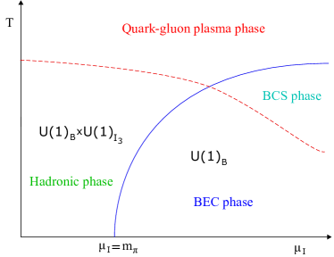
Figure 1: Schematic phase diagram in the $\mu_{I}$–$T$ plane. See main text for details.

For small values of the temperature, and the isospin chemical potential, we are in the confined phase with pionic degrees of freedom. The blue line indicates the transition to a Bose-condensed phase of charged pions, crossing the $\mu_{I}$ axis exactly at $\mu_{I}=m_{\pi}$. The red line indicates the transition to a deconfined phase of quarks and gluons. For small values of $\mu_{I}$, this is a transition from the confined phase. For larger values of $\mu_{I}$ it is a transition from the pion-condensed phase to a BCS phase of weakly interacting quarks that form Cooper pairs son . The latter is a crossover since it is the same $U(1)$-symmetry which is broken in the two cases. Various aspects of the phase diagram at finite $\mu_{I}$ can be found in e.g. Refs. kim ; kogut33 ; loewe ; loewe1 ; njl3f ; qmstiele ; ueda ; lorenz ; 2fabuki ; ebert1 ; ebert2 ; toublannjl ; bar2f ; he2f ; heman2 ; fragaiso ; 2fbuballa ; cohen2 ; carig0 ; carigchpt ; luca ; he3f ; ricardo ; ruggi and a recent review in Ref. mannarev . A first principle dynamical lattice computation of the QCD phase diagram at finite isospin density and temperature for $N_{f}=4+4$ flavors was reported in Ref.  Forcrand . In a series of papers, we have studied the properties of QCD at finite isospin and strange chemical potential at zero temperature using $\chi$PT twoflavor ; us ; condensates . In the case of finite isospin chemical potential and zero strange chemical potential, the predictions from chiral perturbation theory for a number of physical quantities have been in good agreement with recent lattice simulations gergy1 . In the present paper, we generalize our results to finite temperature. The article is organized as follows. In Section 2, we discuss the $\chi$PT Lagrangian, the QCD ground state as a function of isospin chemical potential, and the fluctuations around it. In section 3, the effective potential at next-to-leading order (NLO) including a pionic source as a function of $T$ and $\mu_{I}$ is calculated. In section 4, the quark and pion condensates are derived, while in section 5, we calculate the pressure to next-to-next-to-leading order (NNLO) in $\chi$PT in the symmetric phase. In section 6, we present and discuss our numerical results, including the phase-transition curve separating the normal phase from the pion-condensed phase. We collect a few useful formulas in an Appendix.

2 Chiral Lagrangian, ground state, and fluctuations

The leading order Lagrangian is

$$\mathcal{L}_{2}=\frac{f^{2}}{4}{\rm Tr}\left[\nabla^{\mu}\Sigma^{\dagger}\nabla_{\mu}\Sigma\right]+\frac{f^{2}}{4}{\rm Tr}\left[\chi^{\dagger}\Sigma+\chi\Sigma^{\dagger}\right]\;,$$ (1)

where $\chi=2B_{0}M+2iB_{0}(j_{1}\tau_{1}+j_{2}\tau_{2})$ with $M={\rm diag}(m,m)$, $f$ is the bare pion-decay constant and $2B_{0}m$ is the bare pion mass. Moreover, $\tau_{a}$ are the Pauli matrices and $j_{1}$ and $j_{2}$ are pionic sources which are necessary in order to generate the pion condensate. The field $\Sigma$ is written as

$$\Sigma = L_{\alpha}\Sigma_{\alpha}R^{\dagger}_{\alpha}\;,$$ (2)

where

$$L_{\alpha} = A_{\alpha}UA_{\alpha}^{\dagger}\;,$$ (3)

$$R_{\alpha} = A_{\alpha}^{\dagger}UA_{\alpha}\;,$$ (4)

$$A_{\alpha} = e^{i\frac{\alpha}{2}(\hat{\phi}_{1}\tau_{1}+\hat{\phi}_{2}\tau_{2})}\;,$$ (5)

$$U = e^{i\frac{\phi_{a}\tau_{a}}{2f}}\;,$$ (6)

where the subscript $\alpha$ (at tree level) can be interpreted as a rotation angle of the quark condensate into a pion condensate, and $\hat{\phi}_{i}$ are real parameters. The ground state $\Sigma_{\alpha}$ in the pion-condensed phase can be parametrized as son

$$\Sigma_{\alpha} = \mathbb{1}\cos\alpha+i(\hat{\phi}_{1}\tau_{1}+\hat{\phi}_{2}\tau_{2})\sin\alpha\;,$$ (7)

The parameters satisfy $\hat{\phi}_{1}^{2}+\hat{\phi}_{2}^{2}=1$ so that the ground state is properly normalized, $\Sigma_{\alpha}^{\dagger}\Sigma_{\alpha}=\mathbb{1}$. Without loss of generality, we can choose $\hat{\phi}_{1}=1$, $\hat{\phi}_{2}=0$ and $j_{1}=j$, $j_{2}=0$.

The covariant derivatives at finite isospin are defined as follows

$$\nabla_{\mu}\Sigma \equiv \partial_{\mu}\Sigma-i\left[v_{\mu},\Sigma\right]\;,$$ (8)

$$\nabla_{\mu}\Sigma^{\dagger} = \partial_{\mu}\Sigma^{\dagger}-i[v_{\mu},\Sigma^{\dagger}]\;,$$ (9)

where $v_{\mu}=\delta_{\mu 0}\mu_{I}\frac{\tau_{3}}{2}$ and $\mu_{I}$ is the isospin chemical potential.

The Lagrangian is expanded in powers of the field through quadratic order is

$${\cal L}_{2}^{\rm static} = f^{2}(2B_{0}m_{j})+\frac{1}{2}f^{2}\mu_{I}^{2}\sin^{2}\alpha\;,$$ (10)

$${\cal L}_{2}^{\rm linear} = f\left(-2B_{0}\bar{m}_{j}+\mu_{I}^{2}\sin\alpha\cos\alpha\right)\phi_{1}$$ (11)

$$+f\mu_{I}\sin\alpha\partial_{0}\phi_{2}\;,$$

$${\cal L}_{2}^{\rm quadratic} = \frac{1}{2}\partial_{\mu}\phi_{a}\partial^{\mu}\phi_{a}-\frac{1}{2}m_{a}^{2}\phi_{a}^{2}$$ (12)

$$+\mu_{I}\cos\alpha(\phi_{1}\partial_{0}\phi_{2}-\phi_{2}\partial_{0}\phi_{1})\;.$$

where the source-dependent masses are

$$m_{j} = m\cos\alpha+j\sin\alpha\;,$$ (13)

$$\bar{m}_{j} = m\sin\alpha-j\cos\alpha\;,$$ (14)

$$m_{1}^{2} = 2B_{0}m_{j}-\mu_{I}^{2}\cos{2}\alpha\;,$$ (15)

$$m_{2}^{2} = 2B_{0}m_{j}-\mu_{I}^{2}\cos^{2}\alpha\;,$$ (16)

$$m_{3}^{2} = 2B_{0}m_{j}+\mu_{I}^{2}\sin^{2}\alpha\;.$$ (17)

The inverse propagator in the $\phi_{a}$ basis is

$$D^{-1} =\begin{pmatrix}D^{-1}_{12}&0\\ 0&P^{2}-m_{3}^{2}\end{pmatrix}\;,$$ (18)

$$D^{-1}_{12} =\begin{pmatrix}P^{2}-m_{1}^{2}&ip_{0}m_{12}\\ -ip_{0}m_{12}&P^{2}-m_{2}^{2}\\ \end{pmatrix}\;,$$ (19)

where $m_{12}=2\mu_{I}\cos\alpha$ and $P=(p_{0},p)$ is the four-momentum, $P^{2}=p_{0}^{2}-p^{2}$. The three dispersion relations are determined by the poles of the propagator, and the expressions are

$$E_{\pi^{\pm}}^{2} = p^{2}+\frac{1}{2}\left(m_{1}^{2}+m_{2}^{2}+m_{12}^{2}\right)$$ (20)

$$\pm\frac{1}{2}\sqrt{4p^{2}m_{12}^{2}+(m_{1}^{2}+m_{2}^{2}+m_{12}^{2})^{2}-4m_{1}^{2}m_{2}^{2}}\;,$$

$$E_{\pi^{0}}^{2} = p^{2}+m_{3}^{2}\;.$$ (21)

At next-to-leading order, the chiral Lagrangian contains a number of operators gasser1 , but not all of them contribute in the present case. The operators that we need are

$${\cal L}_{4} = \frac{1}{4}l_{1}\left({\rm Tr}\left[\nabla_{\mu}\Sigma^{\dagger}\nabla^{\mu}\Sigma\right]\right)^{2}$$ (22)

$$+\frac{1}{4}l_{2}{\rm Tr}\left[\nabla_{\mu}\Sigma^{\dagger}\nabla_{\nu}\Sigma\right]{\rm Tr}\left[\nabla^{\mu}\Sigma^{\dagger}\nabla^{\nu}\Sigma\right]$$

$$+\frac{1}{16}(l_{3}+l_{4})({\rm Tr}[\chi^{\dagger}\Sigma+\Sigma^{\dagger}\chi])^{2}$$

$$+\frac{1}{8}l_{4}{\rm Tr}\left[\nabla_{\mu}\Sigma^{\dagger}\nabla^{\mu}\Sigma\right]{\rm Tr}[\chi^{\dagger}\Sigma+\Sigma^{\dagger}\chi]$$

$$+\frac{1}{2}h_{1}{\rm Tr}[\chi^{\dagger}\chi]\;.$$

where $l_{1}$–$l_{4}$ and $h_{1}$ are bare coupling constants. The bare and renormalized couplings $l_{i}^{r}(\Lambda)$, $h_{i}^{r}(\Lambda)$ are related as follows

$$l_{i} = l_{i}^{r}(\Lambda)-\frac{\gamma_{i}\Lambda^{-2\epsilon}}{2(4\pi)^{2}}\left[\frac{1}{\epsilon}+1\right]\;,$$ (23)

$$h_{i} = h_{i}^{r}(\Lambda)-\frac{\delta_{i}\Lambda^{-2\epsilon}}{2(4\pi)^{2}}\left[\frac{1}{\epsilon}+1\right]\;,$$ (24)

where $\gamma_{i}$ and $\delta_{i}$ are coefficients, and $\Lambda$ is the renormalization scale in the modified minimal subtraction ($\overline{\rm MS}$) scheme (see Appendix A). The renormalized couplings $l_{i}^{r}(\Lambda)$ and $h_{i}^{r}(\Lambda)$ are running satisfying a renormalization group equation. Since the bare couplings are independent of the renormalization scale $\Lambda$, differentiation of Eqs. (23) – (24) immediately yields

$$\Lambda{d\over d\Lambda}l_{i}^{r} =-\frac{\gamma_{i}\Lambda^{-2\epsilon}}{(4\pi)^{2}}(1+\epsilon)\;, \Lambda{d\over d\Lambda}h_{i}^{r}=-\frac{\delta_{i}\Lambda^{-2\epsilon}}{(4\pi)^{2}}(1+\epsilon)\;.$$ (25)

The low-energy constants $\bar{l}_{i}$ and $\bar{h}_{1}$ are defined via the solutions to the renormalization group equations (25) for $\epsilon=0$,

$$l_{i}^{r}(\Lambda) = {\gamma_{i}\over 2(4\pi)^{2}}\left[\bar{l}_{i}+\log{M^{2}\over\Lambda^{2}}\right]\;,$$ (26)

$$h_{i}^{r}(\Lambda) = {\delta_{i}\over 2(4\pi)^{2}}\left[\bar{h}_{i}+\log{M^{2}\over\Lambda^{2}}\right]\;,$$ (27)

and are up to a constant equal to the renormalized couplings $l_{i}^{r}(\Lambda)$ and $h_{i}^{r}(\Lambda)$ evaluated at the scale $\Lambda=M$ gasser1 . The coefficients $\gamma_{i}$ and $h_{i}$ are

$$\gamma_{1} = \frac{1}{3}\;,\hskip 8.5359pt\gamma_{2}=\frac{2}{3}\;,\hskip 8.5359pt\gamma_{3}=-\frac{1}{2}\;,$$ (28)

$$\gamma_{4} = 2\;,\hskip 8.5359pt\delta_{1}=0\;.$$ (29)

Since $\delta_{1}=0$, Eq. (27) does not apply and the coupling $h_{1}^{r}$ does not run. In the paper gasser1 , the authors used another minimal set of invariant operators than we have listed in Eq. (22). The two sets of operators can be transformed into each other using equations of motion. The couplings are related as ${h}_{1}=\tilde{h}_{1}-\tilde{l}_{4}$, where the tilde refers to the original couplings scherer . The corresponding values of the relevant $\tilde{\gamma}_{i}$ and $\tilde{\delta}_{i}$ are the same except $\tilde{\delta}_{1}=2$. This implies that $\tilde{h}_{1}^{r}$ runs according to Eq. (27). At ${\cal O}(p^{6})$, there are 53 terms and four contact terms in the $SU(2)$ chiral Lagrangian bijnens0 ; bijnens1 . However, only two terms contribute to the static Lagrangian ${\cal L}_{6}^{\rm static}$ hofmann . Denoting the bare couplings by $c_{i}$, only the sum $16(c_{10}+2c_{11})(2B_{0}m)^{3}$ contributes, where

$$c_{10}+2c_{11} = {\Lambda^{-4\epsilon}(c_{10}^{r}+2c_{11}^{r})\over f^{2}}-{3\Lambda^{-4\epsilon}\over 128(4\pi)^{4}f^{2}}\left[{1\over\epsilon}+1\right]^{2}$$ (30)

$$-{3\Lambda^{-2\epsilon}\over 16(4\pi)^{2}f^{2}}{l}_{3}^{r}\left[{1\over\epsilon}+1\right]\;,$$

and where $c_{i}^{r}(\Lambda)$ are the renormalized couplings. Since the bare couplings $c_{i}$ are independent of the scale $\Lambda$, the sum $c_{10}^{r}(\Lambda)+2c_{11}^{r}(\Lambda)$ satisfies the renormalization group equation ($\epsilon=0$)

$$\Lambda{d(c_{10}^{r}+2c_{11}^{r})\over d\Lambda} = -{3\over 8}{l_{3}^{r}\over(4\pi)^{2}}\;.$$ (31)

Using Eq. (26) with $i=3$, we can write

$$\Lambda{d(c_{10}^{r}+2c_{11}^{r})\over d\Lambda} = {3\over 32(4\pi)^{4}}\left[\bar{l}_{3}+\log{M^{2}\over\Lambda^{2}}\right]\;.$$ (32)

Integrating this equation and defining the constants $\bar{c}_{10}$ and $\bar{c}_{11}$ as the renormalized couplings $c_{10}^{r}$ and $c_{11}^{r}$ at the scale $\Lambda=M$ up to the prefactor $-{3\bar{l}_{3}\over 64(4\pi)^{4}}$ hofmann , we can write

$$c_{10}^{r}(\Lambda)+2c_{11}^{r}(\Lambda) = -{3\bar{l}_{3}\over 64(4\pi)^{4}}(\bar{c}_{10}+2\bar{c}_{11})-{3\bar{l}_{3}\over 64(4\pi)^{4}}\log{M^{2}\over\Lambda^{2}}$$ (33)

$$-{3\over 128(4\pi)^{4}}\log^{2}{M^{2}\over\Lambda^{2}}\;.$$

The one-loop effective potential in the pion-condensed phase receives a static contribution, which is given by minus the static term in Eq. (22),

$$\mathcal{L}_{4}^{\rm static} =(l_{1}+l_{2})\mu_{I}^{4}\sin^{4}\alpha+l_{4}(2B_{0}m_{j})\mu_{I}^{2}\sin^{2}\alpha$$

$$+(l_{3}+l_{4})(2B_{0}m_{j})^{2}+h_{1}\left[(2B_{0}m_{j})^{2}+(2B_{0}\bar{m}_{j})^{2}\right]\;.$$ (34)

In Sec. 5, we will calculate the pressure to order ${\cal O}(p^{6})$ in the symmetric phase, i. e. for $\alpha=0$. In this case the charged eigenstates and the mass eigenstates coincide and it is convenient to use the basis

$$\Phi = {1\over\sqrt{2}}(\phi_{1}+i\phi_{2})\;,\hskip 28.45274pt\Phi^{\dagger}={1\over\sqrt{2}}(\phi_{1}-i\phi_{2})\;,$$ (35)

We then express the Lagrangian in terms of $\Phi$, $\Phi^{\dagger}$, and $\phi_{3}$ instead of $\phi_{a}$. The covariant derivatives in the charged basis are defined in the usual way,

$$D_{\mu}\Phi \equiv(\partial_{\mu}+i\delta_{\mu 0}\mu_{I})\Phi,$$ (36)

$$D_{\mu}\Phi^{\dagger} \equiv(\partial_{\mu}-i\delta_{\mu 0}\mu_{I})\Phi^{\dagger}\;.$$ (37)

The quadratic Lagrangian Eq. (12) then becomes

$${\cal L}^{\rm quadratic}_{2} = D_{\mu}\Phi^{\dagger}D^{\mu}\Phi+{1\over 2}\partial_{\mu}\phi_{3}\partial^{\mu}\phi_{3}$$ (38)

$$-2B_{0}m\Phi^{\dagger}\Phi-{1\over 2}(2B_{0}m)\phi_{3}^{2}\;.$$

The quartic terms from Eq. (1) can be written as,

$${\cal L}_{2}^{\rm quartic} = -{1\over 3f^{2}}\Phi^{\dagger}\Phi\left[D_{\mu}\Phi^{\dagger}D^{\mu}\Phi-B_{0}m\Phi^{\dagger}\Phi\right]$$ (39)

$$-{1\over 3f^{2}}\phi_{3}^{2}\left[D_{\mu}\Phi^{\dagger}D^{\mu}\Phi-2B_{0}m\Phi^{\dagger}\Phi\right]$$

$$-{1\over 6f^{2}}\Phi^{\dagger}\Phi\left[2\partial_{\mu}\phi_{3}\partial^{\mu}\phi_{3}+2B_{0}m\phi_{3}^{2}\right]$$

$$+{1\over 6f^{2}}\left[\Phi\Phi D_{\mu}\Phi^{\dagger}D^{\mu}\Phi^{\dagger}+\Phi^{\dagger}\Phi^{\dagger}D_{\mu}\Phi D^{\mu}\Phi\right]$$

$$+{1\over 6f^{2}}\left(\partial_{\mu}\phi_{3}^{2}\right)\partial^{\mu}\left(\Phi^{\dagger}\Phi\right)+{2B_{0}m\over 24f^{2}}\phi_{3}^{4}\;.$$

The quadratic terms from Eq. (22) are

$${\cal L}_{4}^{\rm quadratic} = {2l_{4}\over f^{2}}\left[D_{\mu}\Phi^{\dagger}D^{\mu}\Phi+\frac{1}{2}\partial_{\mu}\phi_{3}\partial^{\mu}\phi_{3}\right]2B_{0}m$$ (40)

$$-{(l_{3}+l_{4})\over f^{2}}\left[2\Phi^{\dagger}\Phi+\phi_{3}^{2}\right](2B_{0}m)^{2}\;.$$

3 Effective potential with pionic source

In this section, we calculate the effective potential to NLO including a pionic source. At $T=0$, this calculation was carried out in Ref. condensates . It is straightforward to generalize the result to finite temperature and we include the calculation for completeness. We perform the finite-temperature calculations using the imaginary-time formalism. The energy $\omega$ is then replaced by $iP_{0}$, where the (bosonic) Matsubara frequencies are given by $P_{0}=2\pi nT$, $n\in\mathbb{Z}$. The Minkowski-space propagator ${i\over P^{2}-m^{2}}$ is replaced by a Euclidean propagator ${1\over P^{2}+m^{2}}$, where $P^{2}=P_{0}^{2}+p^{2}$. The propagator for the complex field in the symmetric phase is $\Delta={1\over(P_{0}+i\mu_{I})^{2}+p^{2}+M^{2}}$. The source-dependent one-loop contribution to the effective potential can be written as

$$V_{1} = {1\over 2}\hbox{$\sum$}\!\!\!\!\!\!\!\!\int_{P}\log\left[P_{0}^{2}+E_{\pi^{+}}^{2}\right]+{1\over 2}\hbox{$\sum$}\!\!\!\!\!\!\!\!\int_{P}\log\left[P_{0}^{2}+E_{\pi^{-}}^{2}\right]$$ (41)

$$+{1\over 2}\hbox{$\sum$}\!\!\!\!\!\!\!\!\int_{P}\log\left[P_{0}^{2}+E_{\pi^{0}}^{2}\right]$$

$$= {1\over 2}\int_{p}\left[E_{\pi^{+}}+E_{\pi^{-}}+E_{\pi^{0}}\right]+T\int_{p}\log\left[1-e^{-\beta E_{\pi^{+}}}\right]$$

$$+T\int_{p}\log\left[1-e^{-\beta E_{\pi^{-}}}\right]+T\int_{p}\log\left[1-e^{-\beta E_{\pi^{0}}}\right]\;,$$

where the dispersion relations $E_{\pi^{0}}$ and $E_{\pi^{\pm}}$ are given by Eqs. (20)–(21).

The zero-temperature integrals involving the charged excitations cannot be done analytically in dimensional regularization. However, we can isolate the ultraviolet divergences by adding and subtracting appropriate terms that can be calculated in dimensional regularization. The ultraviolet behavior of $E_{\pi^{\pm}}$ is given by $E_{1,2}=\sqrt{p^{2}+m^{2}_{1,2}+{1\over 4}m_{12}^{2}}$, i.e. excitations with masses $\tilde{m}_{1}^{2}=2B_{0}m_{j}+\mu_{I}^{2}\sin^{2}\alpha=m_{3}^{2}$ and $\tilde{m}_{2}^{2}=2B_{0}m_{j}$. We can therefore write

$$V_{1} = V_{1}^{\rm div}+V_{1}^{\rm fin}\;,$$ (42)

where

$$V_{1}^{\rm div} = \int_{p}\sqrt{p^{2}+m_{3}^{2}}+{1\over 2}\int_{p}\sqrt{p^{2}+\tilde{m}_{2}^{2}},$$ (43)

$$= -{1\over 2(4\pi)^{2}}\left[{1\over\epsilon}+{3\over 2}+\log{2B_{0}m\over{m}_{3}^{2}}\right](2B_{0}m_{j}+\mu_{I}^{2}\sin^{2}\alpha)^{2}$$

$$-{1\over 4(4\pi)^{2}}\left[{1\over\epsilon}+{3\over 2}+\log{2B_{0}m\over{\tilde{m}_{2}^{2}}}\right](2B_{0}m_{j})^{2}\;,$$

$$V_{1}^{\rm fin} = {1\over 2}\int_{p}\left[E_{\pi^{+}}+E_{\pi^{-}}-\sqrt{p^{2}+\tilde{m}_{1}^{2}}-\sqrt{p^{2}+\tilde{m}_{2}^{2}}\right]\;.$$ (44)

The complete NLO effective potential is the sum of Eqs. (43)–(44) minus Eqs. (10) and (2). Renormalization is carried out by replacing $l_{i}$ by $l_{r}(\Lambda)$ according to Eqs. (23) and (26).

where we have defined $\bar{h}_{1}=(4\pi)^{2}h_{1}$. We note that the result is independent of $\Lambda$, which implies that thermodynamic functions and condensates that we generate are independent of the renormalization scale.

4 Quark and pion condensates

In Ref. condensates , we derived the quark and pion condensates in the pion-condensed phase at $T=0$. In this section, we generalize the results to finite temperature. We begin with the definition of the chiral condensate and the pion condensate, which are

$$\langle\bar{\psi}\psi\rangle_{\mu_{I}} = {1\over 2}{\partial V_{\rm eff}\over\partial m}\;,\hskip 11.38092pt\langle\pi^{+}\rangle_{\mu_{I}}={1\over 2}{\partial V_{\rm eff}\over\partial j}\;,$$ (46)

respectively, where the subscript is a reminder that the condensates depend on the isospin chemical potential. At leading order the condensates read

$$\langle\bar{\psi}\psi\rangle_{\mu_{I},\rm tree} =-f^{2}B_{0}\cos\alpha\;,$$ (47)

$$\langle\pi^{+}\rangle_{\mu_{I},\rm tree} =-f^{2}B_{0}\sin\alpha\;.$$ (48)

with the pion condensate vanishing in the normal vacuum with $\alpha=0$. The temperature dependence of the effective potential enters through loop corrections, so all tree-level results are temperature independent. Furthermore, we also note that the sum of the square of the condensates is constant,

$$\langle\bar{\psi}\psi\rangle_{\mu_{I},\rm tree}^{2}+\langle\pi^{+}\rangle_{\mu_{I},\rm tree}^{2}=(-f^{2}B_{0})^{2}\;,$$ (49)

with a radius equal to the chiral condensate of the normal vacuum. At NLO, this rotation relation is violated and the condensates can be expressed as

$$\langle\bar{\psi}\psi\rangle_{\mu_{I}} =\langle\bar{\psi}\psi\rangle_{\mu_{I},0}+\langle\bar{\psi}\psi\rangle_{\mu_{I},T}\;,$$ (50)

$$\langle\pi^{+}\rangle_{\mu_{I}} =\langle\pi^{+}\rangle_{\mu_{I},0}+\langle\pi^{+}\rangle_{\mu_{I},T}\;,$$ (51)

where the first terms are the temperature-independent contributions while the second terms are temperature dependent. These contributions are calculated using the effective potential in Eq. (LABEL:renpi). The results below are obtained by first taking the appropriate partial derivatives and then setting the reference scale $M^{2}$ equal to $2B_{0}m$.

The temperature-independent contributions were first calculated in Ref. condensates , while the temperature-dependent contributions are new and follow directly from the last line of Eq. (LABEL:renpi).

5 Two-loop pressure in the symmetric phase

In this section, we calculate the pressure to two-loop order which corresponds to a next-to-next-to-leading order calculation in the low-energy expansion. Through one-loop, the pressure is given by

$${\cal P}_{0+1} = f^{2}(2B_{0}m)+(l_{3}+l_{4})(2B_{0}m)^{2}+h_{1}(2B_{0}m)^{2}$$ (56)

$$-{1\over 2}\hbox{$\sum$}\!\!\!\!\!\!\!\!\int_{Q}\log[Q^{2}+2B_{0}m]$$

$$-\hbox{$\sum$}\!\!\!\!\!\!\!\!\int_{Q}\log[(Q_{0}+i\mu_{I})^{2}+q^{2}+2B_{0}m]\;,$$

where the mean-field term Eq. (10) and the contribution from the counterterm Eq. (2) are evaluated at $\alpha=0$. Here and in the following, the subscript $n$ of ${\cal P}_{n}$ denotes the $n$th order in the low-energy expansion and the subscript $0+1..+n$ denotes the complete result to the same order. Using the expressions for the sum-integral (LABEL:sumint22) as well renormalizing the couplings using Eqs. (23)–(24), and the relation Eq. (26), we obtain the pressure to NLO

$${\cal P}_{0+1} = f^{2}(2B_{0}m)+{(2B_{0}m)^{2}\over 4(4\pi)^{2}}\left[\frac{3}{2}-\bar{l}_{3}+4\bar{l}_{4}+4\bar{h}_{1}\right]$$ (57)

$$-T\int_{q}\left\{\log\left[1-e^{-\beta E_{q}}\right]+\log\left[1-e^{-\beta(E_{q}-\mu_{I})}\right]\right.$$

$$\left.+\log\left[1-e^{-\beta(E_{q}+\mu_{I})}\right]\right\}\;.$$

The first line in Eq. (57) is the vacuum energy, while the second and third line are the pressure of an ideal gas of massive particles of mass $2B_{0}m$ at finite isospin chemical potential.

At NNLO, there are a number of diagrams that contribute to the pressure. The two-loop diagrams arising from ${\cal L}_{2}^{\rm quartic}$, Eq. (39) are shown in the first line of Fig. (2), while the the counterterm diagrams arising from Eq. (40) as well as the contact term are shown in the second line of Fig. (2).

Figure 2: NNLO diagrams for the pressure in the symmetric phase. A solid line corresponds to the charged pion and a dashed line corresponds to the neutral pion. A black dot is a mass insertion or a temperature-independent counterterm.

Using Eqs. (LABEL:sumint22)–(LABEL:sumint33), the two-loop contribution to the pressure can be written as

$${\cal P}_{2}^{\rm quartic} = -{2B_{0}m\over 2f^{2}}\hbox{$\sum$}\!\!\!\!\!\!\!\!\int_{K}{1\over K^{2}+2B_{0}m}\hbox{$\sum$}\!\!\!\!\!\!\!\!\int_{Q}{1\over(Q_{0}+i\mu_{I})^{2}+q^{2}+2B_{0}m}$$ (58)

$$+{2B_{0}m\over 8f^{2}}\left[\hbox{$\sum$}\!\!\!\!\!\!\!\!\int_{Q}{1\over Q^{2}+2B_{0}m}\right]^{2}$$

$$+{1\over f^{2}}\left[\hbox{$\sum$}\!\!\!\!\!\!\!\!\int_{Q}{(Q_{0}+i\mu_{I})\over(Q_{0}+i\mu_{I})^{2}+q^{2}+2B_{0}m}\right]^{2}$$

$$= -{3(2B_{0}m)^{3}\over 8(4\pi)^{4}f^{2}}\left[{1\over\epsilon^{2}}+{2\over\epsilon}\left(1+\log{\Lambda^{2}\over 2B_{0}m}\right)\right.$$

$$\left.+3+{\pi^{2}\over 6}+4\log{\Lambda^{2}\over 2B_{0}m}+2\log^{2}{\Lambda^{2}\over 2B_{0}m}\right]$$

$$+{(2B_{0}m)^{2}\over 4(4\pi)^{2}f^{2}}\left({1\over\epsilon}+1+\log{\Lambda^{2}\over 2B_{0}m}\right)$$

$$\times\int_{q}\left[{n_{B}(E_{q})\over E_{q}}+{n_{B}(E_{q}-\mu_{I})\over E_{q}}+{n_{B}(E_{q}+\mu_{I})\over E_{q}}\right]$$

$$-{2B_{0}m\over 4f^{2}}\int_{q}\left[{n_{B}(E_{q}-\mu_{I})\over E_{q}}+{n_{B}(E_{q}+\mu_{I})\over E_{q}}\right]$$

$$\times\int_{q}{n_{B}(E_{k})\over E_{k}}+{2B_{0}m\over 8f^{2}}\left[\int_{q}{n_{B}(E_{q})\over E_{q}}\right]^{2}$$

$$-{1\over 4f^{2}}\left\{\int_{q}\big{[}n_{B}(E_{q}-\mu_{I})-n_{B}(E_{q}+\mu_{I})\big{]}\right\}^{2}\;.$$

The one-loop counterterm contribution to the pressure ${\cal P}_{2}^{\rm ct}$ from ${\cal L}_{4}^{\rm quadratic}$ is

$${\cal P}_{2}^{\rm ct} = -{l_{3}(2B_{0}m)^{2}\over f^{2}}\hbox{$\sum$}\!\!\!\!\!\!\!\!\int_{Q}\left[{2\over(Q_{0}+i\mu_{I})^{2}+q^{2}+2B_{0}m}+{1\over Q^{2}+2B_{0}m}\right]$$ (59)

$$= \frac{3l_{3}(2B_{0}m)^{3}}{(4\pi)^{2}f^{2}}\left[{1\over\epsilon}+1+\log{\Lambda^{2}\over 2B_{0}m}+{\pi^{2}+12\over 12}\epsilon+\log{\Lambda^{2}\over 2B_{0}m}\epsilon\right.$$

$$\left.+\frac{1}{2}\log^{2}\left(\frac{\Lambda^{2}}{2B_{0}m}\right)\epsilon\right]-{l_{3}(2B_{0}m)^{2}\over f^{2}}$$

$$\times\int_{q}\left[{n_{B}(E_{q})\over E_{q}}+{n_{B}(E_{q}-\mu_{I})\over E_{q}}+{n_{B}(E_{q}+\mu_{I})\over E_{q}}\right]\;,$$

where we have expanded the zero-temperature part of the loop integral to order $\epsilon$ in order to pick up a finite term when it is multiplied by the bare coupling $l_{3}$. Finally, the contact term is

$${\cal P}_{2}^{\rm contact} = 16(c_{10}+2c_{11})(2B_{0}m)^{3}\;.$$ (60)

The NNLO contribution to the pressure is then given by the sum of Eqs. (58), (59), and (60). The ultraviolet divergences are eliminated upon substituting $l_{3}$ by $l_{3}^{r}$ using (26) and $c_{10}+2c_{11}$ by $c_{10}^{r}+2c_{11}^{r}$ using Eq. (30). The running couplings $l_{3}^{r}$ and $c_{10}^{r}+2c_{11}^{r}$ are then replaced by the right-hand side of Eqs. (26) and (33). After adding Eqs. (57)–(60) and renormalizing, we obtain

$${\cal P}_{0+1+2} = f^{2}(2B_{0}m)+{(2B_{0}m)^{2}\over 4(4\pi)^{2}}\left[{3\over 2}-\bar{l}_{3}+4\bar{l}_{4}+4\bar{h}_{1}\right]$$ (61)

$$+{3\bar{l}_{3}(2B_{0}m)^{3}\over 4(4\pi)^{4}f^{2}}\left[\bar{c}_{10}+2\bar{c}_{11}\right]$$

$$-T\int_{q}\left\{\log\left[1-e^{-\beta E_{q}}\right]+\log\left[1-e^{-\beta(E_{q}-\mu_{I})}\right]\right.$$

$$\left.+\log\left[1-e^{-\beta(E_{q}+\mu_{I})}\right]\right\}$$

$${+}{(2B_{0}m)^{2}\over 4(4\pi)^{2}f^{2}}\bar{l}_{3}$$

$$\times\int_{q}\left[{n_{B}(E_{q})\over E_{q}}+{n_{B}(E_{q}-\mu_{I})\over E_{q}}+{n_{B}(E_{q}+\mu_{I})\over E_{q}}\right]$$

$$-{2B_{0}m\over 4f^{2}}\left[\int_{q}{n_{B}(E_{q}-\mu_{I})\over E_{q}}+{n_{B}(E_{q}+\mu_{I})\over E_{q}}\right]$$

$$\times\int_{k}{n_{B}(E_{k})\over E_{k}}+{2B_{0}m\over 8f^{2}}\left[\int_{q}{n_{B}(E_{q})\over E_{q}}\right]^{2}$$

$$-{1\over 4f^{2}}\left\{\int_{q}\big{[}n_{B}(E_{q}-\mu_{I})-n_{B}(E_{q}+\mu_{I})\big{]}\right\}^{2}\;.$$

The term on the third and fourth line can be absorbed in the one-loop result (57) by making the substitution $2B_{0}m\rightarrow m^{2}_{\pi}=2B_{0}m\left(1-{2B_{0}m\over 2(4\pi)^{2}f^{2}}\bar{l}_{3}\right)$, where $m_{\pi}$ is the physical pion mass in the vacuum, at one loop. This can be seen by writing $m_{\pi}^{2}=m^{2}+\delta m^{2}$ and expanding the one-loop result to first order in $\delta m^{2}$. The final result then reads

$${\cal P}_{0+1+2} = f^{2}(2B_{0}m)+{(2B_{0}m)^{2}\over 4(4\pi)^{2}}\left[{3\over 2}-\bar{l}_{3}+4\bar{l}_{4}+4\bar{h}_{1}\right]$$ (62)

$$+{3\bar{l}_{3}(2B_{0}m)^{3}\over 4(4\pi)^{4}f^{2}}\left[\bar{c}_{10}+2\bar{c}_{11}\right]$$

$$-T\int_{q}\left\{\log\left[1-e^{-\beta E_{q}}\right]+\log\left[1-e^{-\beta(E_{q}-\mu_{I})}\right]\right.$$

$$\left.+\log\left[1-e^{-\beta(E_{q}+\mu_{I})}\right]\right\}$$

$$-{2B_{0}m\over 4f^{2}}\int_{q}\left[{n_{B}(E_{q}-\mu_{I})\over E_{q}}+{n_{B}(E_{q}+\mu_{I})\over E_{q}}\right]$$

$$\times\int_{p}{n_{B}(E_{p})\over E_{p}}+{2B_{0}m\over 8f^{2}}\left[\int_{q}{n_{B}(E_{q})\over E_{q}}\right]^{2}$$

$$-{1\over 4f^{2}}\left\{\int_{q}\big{[}n_{B}(E_{q}-\mu_{I})-n_{B}(E_{q}+\mu_{I})\big{]}\right\}^{2}\;.$$

The final result is scale independent. In the limit $\mu_{I}\rightarrow 0$, the temperature-dependent terms of the result Eq. (62) reduce to the result of Gerber and Leutwyler when restricting their three-loop result to two loops gerber . In the chiral limit, it reduces to a gas of noninteracting bosons.  The temperature-independent terms agree with the result first obtained in Ref. hofmann for the full vacuum energy to order ${\cal O}(p^{6})$ in $\chi$PT.

6 Numerical results and discussion

Our results for the quark and pion condensates, and the pressure contain a number parameters from the chiral Lagrangian, namely $2B_{0}m$ and $f$, the four low-energy constants $l_{1}-l_{4}$, and the contact parameter $h_{1}$. The low-energy constants $\bar{l}_{1}$ and $\bar{l}_{2}$ were measured experimentally via $d$-wave scattering lengths, while $\bar{l}_{3}$ has been estimated using three-flavor QCD gasser1 . The low-energy constant $\bar{l}_{4}$ is related to the scalar radius of the pion. We have determined $\bar{h}_{1}$ using the values and uncertainties of the three-flavor low-energy constants in Ref. Hr2ref1 and the mapping of three-flavor LECs to two-flavor LECs as discussed in Ref. gasser2 .  The numerical values are cola

$$\bar{l}_{1} =-0.4\pm 0.6\;, \bar{l}_{2}=4.3\pm 0.1\;,$$ (63)

$$\bar{l}_{3} =2.9\pm 2.4\;, \bar{l}_{4}=4.4\pm 0.2\;,$$ (64)

$$\bar{h}_{1} =-1.5\pm 0.2.$$ (65)

We are aware of more recent values of the low-energy constants newlow , but for consistency, we use the same values as Refs. twoflavor ; us ; condensates to compare $\chi$PT with LQCD at zero temperature. The relations between the bare parameters $f$ and $2B_{0}m$ in the chiral Lagrangian and the physical pion mass $m_{\pi}$ and the pion-decay constant $f_{\pi}$ at one loop are given by gasser1

$$m_{\pi}^{2} = 2B_{0}m\left[1-{2B_{0}m\over 2(4\pi)^{2}f^{2}}\bar{l}_{3}\right]\;,$$ (66)

$$f_{\pi}^{2} = f^{2}\left[1+{4B_{0}m\over(4\pi)^{2}f^{2}}\bar{l}_{4}\right]\;.$$ (67)

Thus once we know the couplings $\bar{l}_{3}$ and $\bar{l}_{4}$ as well as the pion mass and the pion-decay constant, we can determine the parameters $f$ and $2B_{0}m$ in the chiral Lagrangian. As in the previous papers twoflavor ; us ; condensates , we adopt the values of $m_{\pi}$ and $f_{\pi}$ used in the lattice simulations of Refs. gergy1 ; gergy2 ; gergy3 ,

$$m_{\pi} = 131\pm 3{\rm\ MeV}\;,\hskip 28.45274ptf_{\pi}={128\pm 3\over\sqrt{2}}{\rm\ MeV}\;.$$ (68)

In the remainder of the paper, we shall be using only the central values of the parameters. Using the central values of the values quoted above, we obtain the bare values

$$(2B_{0}m)_{\rm cen} = 132.4884\,{\rm\ MeV}\;,\hskip 11.38092ptf_{\rm cen}=84.9342\,{\rm\ MeV}\;.$$ (69)

Using the value (69), we can calculate $B_{0}$ using the continuum value of the quark mass, the bare pion-decay constant and the bare pion mass. Unfortunately, the quark mass is not known for the isospin simulations of Refs. gergy1 ; gergy2 ; gergy3 . We therefore use the continuum value of the quark mass from a different lattice computation BMW , similar to what we did in the zero temperature analysis of Ref condensates . Previously, the zero temperature condensates condensates were found to be insensitive to the values of the continuum quark mass (and their corresponding uncertainties) BMW . The parameters most sensitive to uncertainties were found to be the pion mass and pion-decay constant.

In order to study the phase transition (critical isospin chemical potential as a function of temperature) analytically, we perform a Ginzburg-Landau expansion of the effective potential in powers of $\alpha$ (around $\alpha=0$),

$$V_{\rm GL} = V_{\rm eff}(0)+a_{2}\alpha^{2}+a_{4}\alpha^{4}+...$$ (70)

At $T=0$, the coefficients $a_{i}$ are functions of $\mu_{I}$ and the parameters of the Lagrangian. At finite temperature, there is additional temperature dependence. The critical isospin chemical potential $\mu_{I}^{c}$ as a function of the critical temperature $T^{c}$ is defined as the curve in the phase diagram where $a_{2}$ vanishes. If $a_{4}$ evaluated at a point on the phase-transition curve is larger than zero, then the transition is second order at that point. If $a_{4}$ is smaller than zero, then the transition is first order at that point. Finally, if $a_{4}=0$, it is a tricritical point where the order of the phase transition changes its character from first to second order. In Ref. twoflavor , it was shown that $a_{2}={1\over 2}f_{\pi}^{2}[m_{\pi}^{2}-\mu_{I}^{2}]$ at $T=0$, which yields a critical chemical potential of $\mu_{I}^{c}=m_{\pi}$. At this value of $\mu_{I}$, $a_{4}$ is positive and consequently the transition is second order.

A low-temperature expansion of the effective potential was carried out in Ref. split2 in the context of two-color QCD to find the coefficients $a_{2}$ and $a_{4}$. In the same paper, the authors also applied these techniques to three-color QCD at finite isospin chemical potential within the approximation $(\mu_{I}-m_{\pi})\ll T\ll m_{\pi}$. Using $m_{\pi}=131{\rm\ MeV}$, the approximation holds within the $20\%$ level for $T\leq 26.2{\rm\ MeV}$ and $\frac{\mu_{I}-m_{\pi}}{m_{\pi}}\leq 0.04$, with the bounds halved assuming a $10\%$ threshold. They obtained the following critical isospin chemical potential, where $a_{2}=0$, for two-flavor QCD

$$\mu_{I}^{c}(T) = m_{\pi}+\frac{1}{4f_{\pi}^{2}}\sqrt{\frac{m_{\pi}^{3}T^{3}}{2\pi^{3}}}\zeta\left(\mbox{$3\over 2$}\right).$$ (71)

The authors also obtained a tricritical point, where $a_{2}=a_{4}=0$, at the following temperature

$$T_{\rm tri}=2m_{\pi}\frac{4\pi-\zeta(\frac{1}{2})\zeta(\frac{3}{2})}{3\zeta^{2}(\frac{3}{2})}\approx 1.6m_{\pi}\;.$$ (72)

However, $T_{\rm tri}$ is outside the region of validity of the approximations used to obtain the result.

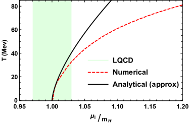
Figure 3: Phase diagram of chiral perturbation theory at finite isospin chemical potential and temperature using the central values of parameters. See main text for details.

A first-order transition is signalled by a jump in the order-parameter $\langle{\pi^{+}}\rangle$. From Eq. (LABEL:pionconfiniteT), it is easily seen that a jump in $\langle{\pi^{+}}\rangle$ can only be generated by a jump in $\alpha$, as long as $\mu_{I}$ and $T$ are continuous variables. Numerically, we do not find any signs of such a jump for temperatures up to $100$ MeV, which is well above the temperature range where the $\chi$PT critical isospin chemical potential agrees with that from lattice QCD. Finally, lattice results gergy3 ; gergy4 as well as model calculations see e.g. heman2 ; njl3f ; allofus find a second-order transition everywhere.

The phase boundary itself is shown in Fig. 3. The red dashed line is the numerical result for the onset of pion condensation as a function of temperature, the solid black line is the analytical result of Eq. (71), and the green shaded area is the lattice QCD result of Refs. gergy3 ; gergy4 . We observe that the red and black curves are in very good agreement for temperatures below $20$ MeV. However, beyond this point there is a significant deviation between the curves, suggesting that the analytical result breaks down rather quickly. While the approximation $(\mu_{I}-m_{\pi})\ll T$ holds quite well along the black curve displayed in Fig. 3 the second approximation $T\ll m_{\pi}$ breaks down somewhere in the lower part of the figure. This elucidates how the discrepancy between the red and black curves can be so significant in the upper region of the figure. Finally, we observe that our numerical result is within the uncertainty range of the lattice data for temperatures up to approximately $35$ MeV. This is contrast to the NJL and quark-meson models that include quark degrees of freedom. The phase boundary predicted by these models heman2 ; allofus is in good agreement with lattice results in the entire temperature range.

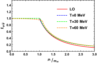
Figure 4: Normalized quark condensate deviation, $\Sigma_{\bar{\psi}\psi}$, as a function of the normalized isospin chemical potential at vanishing and finite temperature to one loop. See main text for details.

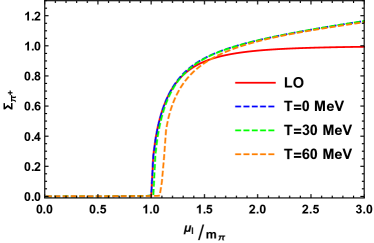
Figure 5: Normalized pion condensate deviation, $\Sigma_{\pi^{+}}$, as a function of the normalized isospin chemical potential at vanishing and finite temperature to one loop. See main text for details.

Let us next turn to the quark and pion condensates. In Ref. condensates we compared the $\chi$PT predictions with those of lattice simulations gergy1 ; gergy2 ; gergy3 at vanishing temperature. The comparison was made between condensate deviations, which characterizes the change of condensate relative to the normal vacuum value. These are defined as

$$\Sigma_{\bar{\psi}\psi} =-\frac{2m}{m_{\pi}^{2}f_{\pi}^{2}}\left[\langle\bar{\psi}\psi\rangle_{\mu_{I}}-\langle\bar{\psi}\psi\rangle_{0}^{j=0}\right]+1\;,$$ (73)

$$\Sigma_{\pi^{+}} =-\frac{2m}{m_{\pi}^{2}f_{\pi}^{2}}\langle\pi^{+}\rangle_{\mu_{I}}\;.$$ (74)

At tree level, the definitions ensure that $\Sigma_{\bar{\psi}\psi}^{2}+\Sigma_{\pi^{+}}^{2}=1$, which simply expresses the rotation (on the chiral circle) of the quark condensate into a pion condensate as $\mu_{I}$ increases. We note that while the subtraction of $\langle\bar{\psi}\psi\rangle_{0}^{j=0}$ in Eq. (73) eliminates the term involving $\bar{h}_{1}$, the definition in Eq. (74) is $\bar{h}_{1}$ dependent. However, the $\bar{h}_{1}$ dependence in Eq. (74) vanishes automatically when we consider the special case, $j=0$, which is what we do in the following.

In Fig 4, we plot $\Sigma_{\bar{\psi}\psi}$ as a function of $\mu_{I}/m_{\pi}$ for three different temperatures. We also include the leading order result in red valid at $T=0$. The blue line indicates the NLO result at $T=0$, the green line shows the $T=30$ MeV result, and the orange line shows the $T=60$ MeV result. We observe that the magnitude of the chiral condensate decreases as we increase the temperature in the normal phase, as expected. Furthermore, the magnitude of $\Sigma_{\bar{\psi}\psi}$ drops significantly once we enter the pion-condensed phase. We also note that for $T=60$ MeV, the chiral condensate starts decreasing due to thermal effects before the second order phase transition occurs. Furthermore, for a fixed isospin chemical potential the chiral condensate increases with temperature. This occurs due to the delayed onset of pion condensation at higher temperatures. Finally, we note that the chiral condensate deviations at different temperatures approach each other at high isospin densities, where finite-density effects dominate over finite-temperature effects. We observe that including finite-temperature effects for temperatures up to $60$ MeV in $\chi$PT to one loop does not lead to very significant corrections to the zero-temperature result in any part of the phase diagram.

In Fig. 5, we show $\Sigma_{\pi^{+}}$ as a function of $\mu_{I}/m_{\pi}$ for three different values of the temperature $T$. The red line shows the $T=0$ MeV LO result, the blue line shows the $T=0$ MeV NLO result, the green line shows the $T=30$ MeV NLO result, and the orange line shows the $T=60$ MeV NLO result. The green and the blue line are barely distinguishable. The difference between the red line and the orange line in the proximity of the phase transition is quite clear and reflects the pronounced temperature dependence that the phase-transition curve attains at high temperatures in $\chi$PT to one loop, as was clearly shown in Fig. 3. Once again we observe that finite-temperature effects become unimportant at large isospin densities. The violation of the relation (49) is clearly seen in Figs. 4– 5 and it has also been observed on the lattice gergy3 . Generally, the agreement between lattice results $\chi$PT at $T=0$ improves as one goes from LO to NLO condensates .

Finally, in Fig. 6, we show the pressure divided by the Stefan-Boltzmann result $P_{\rm{SB}}={T^{4}\pi^{2}\over 30}$ as a function of $T/m_{\pi}$ for three different values of the isospin chemical potential. From above, $\mu_{I}=0$, $\mu_{I}={1\over 4}m_{\pi}$, and $\mu_{I}={1\over 2}m_{\pi}$. The pressure at $T=0$ has been subtracted. The solid lines are the one-loop results, while the black dashed lines display the two-loop result. The low-energy expansion seems to be converging very well. The good convergence properties of the low-energy expansion were also found for the quark condensate up to three loops at $\mu_{I}=0$ gerber .

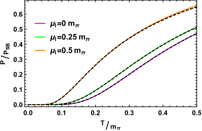
Figure 6: Pressure normalized to the Stefan-Boltzmann pressure as a function of $T/m_{\pi}$ for three different values of $\mu_{I}$. See main text for details.

While it is clear that $\chi$PT is breaking down at some temperature below the deconfinement temperature simply because it only incorporates mesonic degrees of freedom, rigorous statements about the validity of our calculations seems difficult since there are several scales involved, namely $m_{\pi}$, $f_{\pi}$, $T$, and $\mu_{I}$. Considering the green band in Fig. 3, comparing $\chi$PT and lattice QCD, suggests that $\chi$PT ceases to be valid at approximately 40 MeV near the phase transition to the pion-condensed phase. A more conservative estimate would be half of this, 20 MeV, where our result for the phase-transition curve is in very good agreement with the analytical approximation of Ref. split2 .

Appendix A Integrals and Sum-integrals

The sum-integral is defined as

$$\hbox{$\sum$}\!\!\!\!\!\!\!\!\int_{P} = T\sum_{n}\int_{p}=T\sum_{n}\left({e^{\gamma_{E}}\Lambda^{2}\over 4\pi}\right)^{\epsilon}\int{d^{d}p\over(2\pi)^{d}}\;,$$ (75)

where the sum is over the Matsubara frequencies $P_{0}=2\pi nT$. The integral over three-momenta is regularized using dimensional regularization with $d=3-2\epsilon$, where $\Lambda$ is a renormalization scale associated with the $\overline{\rm MS}$ scheme. In dimensional regularization, we find

$$\int_{p}\sqrt{p^{2}+m^{2}} = -{m^{4}\over 2(4\pi)^{2}}\left({\Lambda^{2}\over m^{2}}\right)^{\epsilon}\left[{1\over\epsilon}+{3\over 2}+{\cal O}(\epsilon)\right]\;.$$ (76)

where $n_{B}(x)={1\over e^{\beta x}-1}$ is the Bose-Einstein distribution function and $E_{p}=\sqrt{p^{2}+m^{2}}$. The sum over Matsubara frequencies in the sum-integrals can be performed using contour integration with standard techniques, see e.g. Ref. kapusta for details. We note that the sum-integral in Eq. (LABEL:sumint33) is finite, and vanishes in the limit $\mu_{I}\rightarrow 0$ since it is odd in the variable $P_{0}$.

References

• (1) K. Rajagopal and F. Wilczek, At the frontier of particle physics, Vol. 3 (World Scientific, Singapore, p 2061) (2001).
• (2) M. G. Alford, A. Schmitt, K. Rajagopal, and T. Schäfer, Rev. Mod. Phys. 80, 1455 (2008).
• (3) K. Fukushima and T. Hatsuda, Rept. Prog. Phys. 74, 014001 (2011).
• (4) L. McLerran and R. D. Pisarski, Nucl. Phys. A 796 83 (2007).
• (5) S. Weinberg, Physica A 96, 327 (1979).
• (6) J. Gasser and H. Leutwyler, Ann. Phys. 158, (142) (1984).
• (7) J. Gasser and H. Leutwyler, Nucl. Phys. B 250, 465 (1985).
• (8) J. Bijnens, G. Colangelo, and G. Ecker, JHEP 02 020 (1999).
• (9) J. B. Kogut and D. K. Sinclair, Phys. Rev. D 66, 014508 (2002).
• (10) J. B. Kogut and D. K. Sinclair, Phys. Rev D 66 034505 (2002).
• (11) J. B. Kogut and D. K. Sinclair, Phys. Rev D 70 094501 (2004).
• (12) D. K. Sinclair and J. B. Kogut, PosLat 2006 147 (2006).
• (13) D. K. Sinclair, J. B. Kogut, PoSLAT 2007 225 (2007).
• (14) B. B. Brandt and G. Endrődi, PoS LATTICE 2016, 039 (2016).
• (15) B. B. Brandt, G. Endrődi, and S. Schmalzbauer, EPJ Web Conf. 175, 07020 (2018).
• (16) B. B. Brandt, G. Endrődi, and S. Schmalzbauer, Phys. Rev. D 97, 054514 (2018).
• (17) B. B. Brandt and G. Endrődi Phys. Rev. D 99, 014518 (2019)
• (18) D. T. Son and M. A. Stephanov, Phys. Rev. Lett. 86, 592 (2001).
• (19) K. Splittorff, D. T. Son, M. A. Stephanov, Phys. Rev. D 64, 016003 (2001).
• (20) J. B. Kogut and D. Toublan, Phys. Rev. D 64 (2001) 034007.
• (21) M. Loewe and C. Villavicencio, Phys. Rev. D 67, 074034 (2003).
• (22) M. Loewe and C. Villavicencio, Phys. Rev. D 70 074005 (2004).
• (23) E. S. Fraga, L. F. Palhares and C. Villavicencio, Phys. Rev. D 79, 014021 (2009).
• (24) T. D. Cohen and S. Sen, Nucl. Phys. A 942, 39 (2015).
• (25) S. Carignano, A. Mammarella, and M. Mannarelli, Phys. Rev. D 93, 051503 (2016).
• (26) S. Carignano, L. Lepori, A. Mammarella, M. Mannarelli and G. Pagliaroli, Eur. Phys. J. A 53, 35 (2017).
• (27) L. Lepori and M. Mannarelli, Phys. Rev. D 99, 096011 (2019).
• (28) T. Xia, L. He, and P. Zhuang, Phys. Rev. D 88, 056013 (2013).
• (29) S. S. Avancini, A. Bandyopadhyay, D. C. Duarte, and R. L.S. Farias, Phys. Rev. D 100 11, 116002 (2019).
• (30) Z.-Y. Lu, C.-J. Xia, and M. Ruggieri, Eur. Phys. J. C 80 1, 46 (2020).
• (31) M. Frank, M. Buballa, and M. Oertel, Phys. Lett. B 562, 221 (2003).
• (32) D. Toublan, and J. B. Kogut, Phys. Lett. B 564, 212 (2003).
• (33) A. Barducci, R. Casalbuoni, G. Pettini, and L. Ravagli Phys. Rev. D 69, 096004 (2004).
• (34) L. He, and P.-F. Zhuang, Phys. Lett. B 615, 93 (2005).
• (35) A. Barducci, R. Casalbuoni, G. Pettini, L. Ravagli, Phys. Rev. D 71, 016011 (2005).
• (36) L. He, M. Jin and P.-F. Zhuang, Phys. Rev. D 71, 116001, (2005).
• (37) D. Ebert and K. G. Klimenko, J. Phys. G 32, 599 (2006).
• (38) D. Ebert and K. G. Klimenko, Eur. Phys. J. C 46, 771 (2006).
• (39) H. Abuki, R. Anglani, R. Gatto, M. Pellicoro, and M. Ruggieri, Phys. Rev. D 79, 034032 (2009).
• (40) K. Kamikado, N. Strodthoff, L. von Smekal, and J. Wambach Phys. Lett. B 718, 1044 (2013).
• (41) H. Ueda, T. Z. Nakano, A. Ohnishi, M. Ruggieri, and K. Sumiyoshi, Phys. Rev. D 88, 074006 (2013).
• (42) R. Stiele, E. S. Fraga and J. Schaffner-Bielich, Phys. Lett. B 729, 72 (2014).
• (43) M. Mannarelli, Particles 2, 411 (2019).
• (44) Ph. de Forcrand, M. A. Stephanov and U. Wenger, PoS LAT 2007 237 (2007)
• (45) P. Adhikari, J. O. Andersen, P. Kneschke, Eur. Phys. J. C 79, 874 (2019).
• (46) P. Adhikari and J. O. Andersen, Phys. Lett. B 804, 135352 (2020); JHEP 06, 170 (2020).
• (47) P. Adhikari and J. O. Andersen, Eur. Phys. J. C 80, 1028 (2020).
• (48) S. Scherer, Adv. Nucl. Phys. 27, 277 (2003).
• (49) J. Bijnens, G. Colangelo, and G. Ecker, Ann. Phys. 280, 100 (2000).
• (50) C. P. Hofmann, Phys. Rev. D 102, 094010 (2020).
• (51) P. Gerber and H. Leutwyler, Nucl. Phys. B 321, 387, (1989).
• (52) M. Jamin, Phys. Lett. B 538, 71 (2002).
• (53) G. Colangelo, J. Gasser, and H. Leutwyler, Nucl. Phys. B 603, 125 (2001).
• (54) S. Aoki et al, Eur. Phys. J. C80, 113 (2020).
• (55) BMW Collaboration, S. Durr, Z. Fodor, C. Hoelbling, S. D. Katz, S. Krieg, T. Kurth, L. Lellouch, T. Lippert, K. K. Szabo and G. Vulvert, Phys. Lett. B, 701, 265 (2011).
• (56) K. Splittorff, D. Toublan, and J. J. M. Verbaarschot, Nucl. Phys. B 620, 290 (2002).
• (57) P. Adhikari, J. O. Andersen, P. Kneschke, Phys. Rev. D 98, 074016 (2018).
• (58) J. I. Kapusta and C. Gale, Finite-Temperature Field Theory, Cambridge University Press, second edition 2006.