Design-Based Inference for Spatial Experiments under Unknown Interference

Ye Wang, Cyrus Samii, Haoge Chang, and P. M. Aronow Wang is Assistant Professor, Department of Political Science, University of North Carolina, Chapel Hill, (Email: yewang@unc.edu). Samii (contact author) is Associate Professor, Department of Politics, New York University (Email: cds2083@nyu.edu). Chang is PhD. Candidate, Department of Economics, Yale University (Email: haoge.chang@yale.edu). Aronow is Associate Professor, Departments of Political Science and Biostatistics, Yale University (Email: p.aronow@yale.edu). For their comments and suggestions, we thank Kirill Borusyak, Stephen Cole, Alexander Demin, Naoki Egami, Jiawei Fu, Michael Hudgens, Peter Hull, Molly Roberts, Fredrik Sävje, Davide Viviano, and seminar participants at Harris School at University of Chicago, New York University Abu Dhabi, Princeton University, Rochester University, Texas A&M., UNC, and UCSD
Abstract

We consider design-based causal inference in settings where randomized treatments have effects that bleed out into space in complex ways that overlap and in violation of the standard “no interference” assumption for many causal inference methods. We define a spatial “average marginalized effect,” which characterizes how, in expectation, units of observation that are a specified distance from an intervention node are affected by treatment at that node, averaging over effects emanating from other intervention nodes. We establish conditions for non-parametric identification under unknown interference, asymptotic distributions of estimators, and recovery of structural effects. We propose methods for both sample-theoretic and permutation-based inference. We provide illustrations using randomized field experiments on forest conservation and health.
Keywords: causal inference, design-based inference, experiments, interference, spatial statistics.

Design-Based Inference for Spatial Experiments under Unknown Interference

1 Introduction

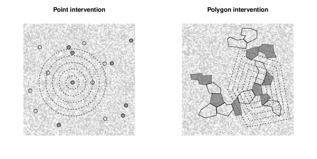
Consider an experiment where an intervention is randomly assigned to specific points or polygons in a geographic space. Then, we observe how outcomes are distributed over this geography. Figure 1 illustrates the generic structure of such experiments. The left panel presents a potential point-intervention experiment. The points are locations at which an intervention might be applied. An experimental design could treat half of such points to receive the intervention (gray shaded points), with the rest of the points remaining in a control condition without intervention (unshaded points). The shading in the background raster indicates outcome values. The right panel illustrates a similar situation, but with interventions assigned to polygons instead of points.

For point interventions, a standard way to analyze such experiments is to, first, define the units of observation as the areas in the immediate vicinity of points of intervention, and then the treatment status of the intervention point defines the treatment status of the areal unit. For polygon interventions, the polygons themselves are the units of observation. Then, the difference in average outcomes across treated versus control units is taken to be an estimate of the average treatment effect (ATE). A key identifying assumption is that potential outcomes for a given unit depend only on the treatment status of that unit (e.g., the nearest site of intervention in the case of point interventions) (Imbens and Rubin, 2015, p. 10). A recent example is Jayachandran et al. (2017), who study a forest conservation experiment by comparing forest cover outcomes in and around villages that hosted a conservation intervention to those that did not.

The problem is that this difference in means does not equal the ATE when the effect of intervening at a given point or polygon bleeds out into other areas since potential outcomes depend not only on a unit’s own treatment status (Halloran and Struchiner, 1995). It is often reasonable to expect such spill-over effects. Incentives provided by a forest conservation intervention may motivate villagers to displace deforestation, causing it to decrease near the boundary of the villages, but then to increase further away. The displacement effect from one village may interact with the effect from another village, making the overall effects complex. We can imagine similarly complex spatial effects from other types of interventions. Vaccination campaigns can have spatial effects on disease prevalence through herd immunity. Product campaigns can have spatial effects on consumer behavior by word-of-mouth or strategic responses of other firms. The dashed lines in Figure 1 display possible zones into which effects may bleed out in our hypothetical examples. Such spatial effects are instances of “interference,” whereby a unit’s potential outcomes depend not only on that unit’s treatment status but rather on the overall distribution of treatments (Cox, 1958, p. 19).
Refer to caption
Figure 1: Illustrations of hypothetical spatial experiments in which interventions are applied to points (left) or polygons (right). The background raster captures the geographic outcome data. We allow for the possibility for effects to bleed out in space, as illustrated by the concentric dashed lines.

This paper develops design-based methods for accounting for such interference in analyzing spatial experiments. Design-based methods derive causal and statistical inferential properties from the experimental design, which is typically under the control of the analyst. We show that when interference is present, rather than estimating the ATE, contrasts between treated and control areas capture a more nuanced, but nonetheless, policy-relevant quantity that we call the “average marginalized effect” (AME).111Previous versions of this paper used “average marginalized response,” but we revised the terminology since “response” is often used in the literature to refer to potential outcomes, rather than effects. We can define AMEs at different distance intervals from where the intervention is applied. The AME is similar to the average direct effect of Halloran and Struchiner (1995) (see also Hudgens and Halloran (2008), VanderWeele and Tchetgen (2011), Sävje et al. (2021), Li and Wager (2022), and Hu et al. (2022)), except that it is indexed by distance for application to the spatial case. The AME measures how, on average, outcomes within the specified distance interval from an intervention node are affected by activating a treatment at that node, taking into account ambient effects emanating from treatments at other intervention nodes. There is a direct mapping from the AME to the types of effects that are assumed by parametric models of spatial effects: when effects emanating from different intervention nodes are additive, the AME recovers the average of these additive effects. If spatial effects are not simply additive but exhibit complex interactions, the AME still yields an interpretable and policy-relevant quantity.

Inference also needs to account for the dependencies that interference creates. We work with a Horvitz-Thompson estimator, a Hajek estimator, and a kernel regression estimator for the AME. We show that these estimators are consistent and asymptotically normal under weak restrictions on the degree of interdependence induced by interference. We further prove that the commonly-used spatial heteroscedasticity and autocorrelation consistent (HAC) variance estimator of Conley (1999) provides conservative estimates for the true variance of these estimators under conditions that are often satisfied in practice.

Our analysis is related to a few streams of current methodological research. First, our approach draws most directly on recent design-based analyses of causal effects under interference that consider estimands marginalized over the randomization distribution, as in Hudgens and Halloran (2008), Sävje et al. (2021), Papadogeorgou et al. (2020), Li and Wager (2022), and Hu et al. (2022). As in these approaches, our inference does not require that we specify the precise structure of the interference network (i.e., the “exposure mapping”, following Aronow and Samii (2017)). It also skirts the issue of non-overlap caused by defining the estimand using the potentially high-dimensional treatment exposure (Leung, 2022b). Second, our analysis is related to recent work on non-parametric estimation of spatial effects, including work on “bipartite causal inference” by Zigler and Papadogeorgou (2018) and on cluster-randomized designs by Leung (2022b). These works focus on cases where points of intervention are far enough apart to yield disjoint clusters that interfere with each other minimally. Such designs are appealing, but they are not always feasible. Similar to m𝑚m-dependence for a time series, we assume hard limits on the extent of interference, but we do not assume that the set of units can be partitioned into a set of disjoint clusters with tractable interference-induced dependencies between any of them. Third, our inferential results rely on the contributions of Ogburn et al. (2020). We also draw connections to inferential results in the spatial econometrics literature (Arbia, 2006; Jenish, 2016; Kelejian and Piras, 2017). We justify the usage of regression estimators in the spatial setting from the design-based perspective and provide causal interpretations for the coefficients. We clarify the connection to Conley (1999)’s spatial HAC variance estimator.

We begin by developing the formal inferential setting and main theoretical results, using a simple toy example to illustrate concepts. We then develop a number of extensions and refinements. We provide simulation evidence of the performance of our proposed estimators and then turn to applications based on experiments in public health and forest conservation.

2 Setting

Suppose a set of intervention nodes 𝒩={1,,N}𝒩1𝑁\mathcal{N}=\{1,...,N\}. Each node i𝒩𝑖𝒩i\in\mathcal{N} can be either a point or a collection of points (e.g., a polygon) that resides in a two-dimensional set 𝒳𝒳\mathcal{X} indexed by x=(x1,x2)𝑥subscript𝑥1subscript𝑥2x=(x_{1},x_{2}) (e.g., latitude and longitude). An experimental design assigns a binary treatment Zi{0,1}subscript𝑍𝑖01Z_{i}\in\{0,1\} to each intervention node. The ordered vector of experimental assignment variables is 𝐙(Z1,,ZN)𝐙subscript𝑍1subscript𝑍𝑁\mathbf{Z}\equiv(Z_{1},...,Z_{N}), and the ex post realized assignment from the experiment is given by 𝐳(z1,,zN)𝐳subscript𝑧1subscript𝑧𝑁\mathbf{z}\equiv(z_{1},...,z_{N}). The experimental design fixes the set of possible assignment vectors 𝒵𝒵\mathcal{Z} as well as a probability distribution over that set, 𝐳subscript𝐳\mathbb{P}_{\mathbf{z}}. Our analysis below considers the case of an experimental design based on Bernouilli randomization for each Zisubscript𝑍𝑖Z_{i}—i.e., (possibly weighted) coin flips to determine treatment status at each node. Analogous to the relationship between sampling with and without replacement, Bernoulli assignment is also a reasonable, if typically conservative, inferential approximation for completely randomized designs when N𝑁N is large. We discuss other differences between Bernoulli and completely randomized designs below.

Potential outcomes at any point x𝒳𝑥𝒳x\in\mathcal{X} are defined for each value of 𝐳𝐳\mathbf{z}, (Yx(𝐳))𝐳𝒵subscriptsubscript𝑌𝑥𝐳𝐳𝒵(Y_{x}(\mathbf{z}))_{\mathbf{z}\in\mathcal{Z}}. Given a realized treatment assignment, 𝐳𝐳\mathbf{z}, we observe the corresponding potential outcome at x𝑥x:

Yx=𝐳𝒵Yx(𝐳)I(𝐙=𝐳).subscript𝑌𝑥subscript𝐳𝒵subscript𝑌𝑥𝐳𝐼𝐙𝐳Y_{x}=\sum_{\mathbf{z}\in\mathcal{Z}}Y_{x}(\mathbf{z})I(\mathbf{Z}=\mathbf{z}).

Data for points in 𝒳𝒳\mathcal{X} may come in various formats including raster data or data for a discrete set of points in 𝒳𝒳\mathcal{X}. Let 𝐘(𝐳)=(Yx(𝐳))x𝒳𝐘𝐳subscriptsubscript𝑌𝑥𝐳𝑥𝒳\mathbf{Y}(\mathbf{z})=(Y_{x}(\mathbf{z}))_{x\in\mathcal{X}} denote the full set of potential outcomes when 𝐙=𝐳𝐙𝐳\mathbf{Z}=\mathbf{z} and 𝐘=(Yx(𝐙))x𝒳𝐘subscriptsubscript𝑌𝑥𝐙𝑥𝒳\mathbf{Y}=(Y_{x}(\mathbf{Z}))_{x\in\mathcal{X}} denote the full set of realized outcomes.

We map the full set of potential outcomes 𝐘(𝐳)𝐘𝐳\mathbf{Y}(\mathbf{z}) for all points in the outcome space 𝒳𝒳\mathcal{X} back to the intervention nodes in 𝒩𝒩\mathcal{N} by defining the “circle average” function:

μi(𝐘(𝐳);Ωd)=1|{x:di(x)Ωd}|x:di(x)ΩdYx(𝐳)dζ.subscript𝜇𝑖𝐘𝐳subscriptΩ𝑑1conditional-set𝑥subscript𝑑𝑖𝑥subscriptΩ𝑑subscript:𝑥subscript𝑑𝑖𝑥subscriptΩ𝑑subscript𝑌𝑥𝐳d𝜁\mu_{i}(\mathbf{Y}(\mathbf{z});\Omega_{d})=\frac{1}{|\{x:d_{i}(x)\in\Omega_{d}\}|}\int_{x:d_{i}(x)\in\Omega_{d}}Y_{x}(\mathbf{z})\text{d}\zeta.

In the expression above, di(x)subscript𝑑𝑖𝑥d_{i}(x) measures the distance between point x𝑥x and intervention node i𝑖i. When i𝑖i is a point located at x(i)𝑥𝑖x(i), di(x)=x(i)xsubscript𝑑𝑖𝑥norm𝑥𝑖𝑥d_{i}(x)=||x(i)-x||, where ||||||\cdot|| is some well-defined metric (e.g., Euclidean or a least-cost distance). If i𝑖i is a collection of points, then di(x)=minxixxsubscript𝑑𝑖𝑥subscriptsuperscript𝑥𝑖normsuperscript𝑥𝑥d_{i}(x)=\min_{x^{\prime}\in i}||x^{\prime}-x||, the minimal distance between x𝑥x and points belonging to i𝑖i. ΩdsubscriptΩ𝑑\Omega_{d} is a set of distance values and ζ𝜁\zeta is a suitable measure on 𝒳𝒳\mathcal{X}. Therefore, μi(𝐘(𝐳);Ωd)subscript𝜇𝑖𝐘𝐳subscriptΩ𝑑\mu_{i}(\mathbf{Y}(\mathbf{z});\Omega_{d}) is the average outcome across points whose distance to i𝑖i falls in ΩdsubscriptΩ𝑑\Omega_{d}. If the points in 𝒳𝒳\mathcal{X} are dense and spaced evenly, then ΩdsubscriptΩ𝑑\Omega_{d} could be a singleton: {di(x):di(x)=d}conditional-setsubscript𝑑𝑖𝑥subscript𝑑𝑖𝑥𝑑\{d_{i}(x):d_{i}(x)=d\}. The circle average amounts to taking the average across points along the edge of a circle of radius d𝑑d around i𝑖i. If the points are spaced such that there are few or no points precisely at the edge of the circle, ΩdsubscriptΩ𝑑\Omega_{d} could be a “donut,” {di(x):dκ<di(x)d}conditional-setsubscript𝑑𝑖𝑥𝑑𝜅subscript𝑑𝑖𝑥𝑑\{d_{i}(x):d-\kappa<d_{i}(x)\leq d\},222κ𝜅\kappa is a user-chosen constant the dictates the donut’s thickness. or a “disk,” {di(x):di(x)d}conditional-setsubscript𝑑𝑖𝑥subscript𝑑𝑖𝑥𝑑\{d_{i}(x):d_{i}(x)\leq d\}. By considering a collection of disjoint sets, {Ωd}d𝒟subscriptsubscriptΩ𝑑𝑑𝒟\{\Omega_{d}\}_{d\in\mathcal{D}}, we will be able to examine how the circle average’s value varies over the geography.333Note that we do not require the union of {Ωd}d𝒟subscriptsubscriptΩ𝑑𝑑𝒟\{\Omega_{d}\}_{d\in\mathcal{D}} to be the entire geography although we do not exclude this possibility either. When it does not cause confusion, we write μi(𝐘(𝐳);Ωd)subscript𝜇𝑖𝐘𝐳subscriptΩ𝑑\mu_{i}(\mathbf{Y}(\mathbf{z});\Omega_{d}) simply as μi(𝐘(𝐳);d)subscript𝜇𝑖𝐘𝐳𝑑\mu_{i}(\mathbf{Y}(\mathbf{z});d). Similarly, the realized circle average for intervention node i𝑖i at d𝑑d is

μi(𝐘;d)=𝐳𝒵μi(𝐘(𝐳);d)I(𝐙=𝐳).subscript𝜇𝑖𝐘𝑑subscript𝐳𝒵subscript𝜇𝑖𝐘𝐳𝑑𝐼𝐙𝐳\mu_{i}(\mathbf{Y};d)=\sum_{\mathbf{z}\in\mathcal{Z}}\mu_{i}(\mathbf{Y}(\mathbf{z});d)I(\mathbf{Z}=\mathbf{z}).

This representation allows us to see how an experiment is a process of sampling potential circle averages for intervention nodes, and therefore allows us to apply sample theoretic (in particular, Horvitz-Thompson- and Hajek-type) results in our analysis below.

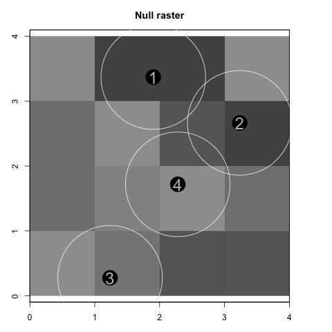
The left plot in Figure 2 illustrates a toy example with a point intervention (N=4𝑁4N=4) and raster outcome data. The plot shows a “null raster” for which none of the intervention nodes has been assigned to treatment and so 𝐳=(0,0,0,0)𝐳0000\mathbf{z}=(0,0,0,0), in which case outcomes are Yx(0,0,0,0)subscript𝑌𝑥0000Y_{x}(0,0,0,0) for all x𝑥x in the space. As we can see, outcomes are defined for any point x𝑥x in the space, although outcomes are constant within raster cells. This is a feature of raster data. Other types of data may exhibit finer levels of granularity — e.g., data produced from kriging interpolation that varies smoothly in space. We take these outcome data, and any coarsening or smoothing operations that they incorporate, as fixed. For our design-based inference, the only source of stochastic variation is from 𝐙𝐙\mathbf{Z}.444For data that are smoothed using kriging, we would tune smoothing parameters on auxiliary data so that they are fixed with respect to 𝐙𝐙\mathbf{Z}. White circles around the intervention nodes demonstrate one possible way to construct the circle average. We use the Euclidean distance and take averages across all the raster cells passed by the edge of the circles. Note that we do not prohibit circles around different nodes to intersect with each other.
Refer to caption
Refer to caption
Figure 2: Left: Illustration of a “null raster,” with N=4𝑁4N=4 intervention nodes (points), none of which are assigned to treatment. The coloring of the raster cells corresponds to outcome levels. White circles around the nodes are circle averages based on the Euclidean distance. Right: Illustration of a possible effect function such that treatments transmit effects non-monotonically in distance. When multiple intervention nodes are treated, these effects accumulate.

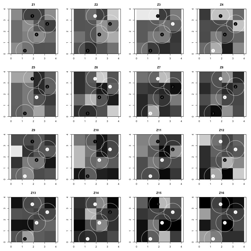
As discussed above, spatial effects can exhibit considerable complexity. For the sake of illustration, suppose in our toy example that treatments tend to transmit effects that are non-monotonic in distance and that these effects simply accumulate in an additive manner. The right plot in Figure 2 illustrates such an effect function. Then, the net result would depend on how treatments are distributed over the intervention points. Figure 3 illustrates how outcomes would be affected over different allocations of the treatment given that effects take the form as in Figure 2. We emphasize that in the analysis below, we do not assume that effects are additive or homogenous in form—this is done here merely to provide a simple illustration.
Refer to caption
Figure 3: Illustration of how outcomes are affected given different allocations of treatment and effects that take the form as presented in the right plot of Figure 2. Treated intervention points are white, while non-treated intervention points are black.

3 Defining a marginal spatial effect

As the potential outcome notation for Yx(𝐳)subscript𝑌𝑥𝐳Y_{x}(\mathbf{z}) indicates, the outcome at any point may depend on the full vector of realized treatment assignments, 𝐳𝐳\mathbf{z}. Similarly, the potential outcome notation for the circle average, μi(𝐘(𝐳);d)subscript𝜇𝑖𝐘𝐳𝑑\mu_{i}(\mathbf{Y}(\mathbf{z});d), suggests that the realized circle average for node i𝑖i may depend on treatment assignments for nodes other than i𝑖i. As such, the circle averages are potentially subject to causal interference.

We now define a spatial effect that we call the “average marginalized effect” (AME). The AME accounts for interference. It is a marginal effect (Rubin, 2005) that bears resemblance to the “average direct effect” of Halloran and Struchiner (1995) and the “average direct causal effect” defined by Hudgens and Halloran (2008) and is a spatial analogue of the “expected average treatment effect” defined by Sävje et al. (2021) or the “average indirect effect” in Hu et al. (2022). The usual definition of a unit-level treatment effect takes the difference between a unit’s potential outcomes under one treatment condition versus under another treatment condition. A unit-level marginal effect is different because it takes the difference between the average of a unit’s potential outcomes over a set of potential outcomes versus the average over another set. We apply this idea to the spatial setting. In doing so, we consider effects that may bleed out in ways that are not necessarily contained within pre-defined strata, as in Hudgens and Halloran (2008).

To define the spatial AME, first rewrite the potential outcome at point x𝑥x as Yx(zi,𝐳i)subscript𝑌𝑥subscript𝑧𝑖subscript𝐳𝑖Y_{x}(z_{i},\mathbf{z}_{-i}), where 𝐳isubscript𝐳𝑖\mathbf{z}_{-i} is a vector equalling 𝐳𝐳\mathbf{z} except that the value for intervention node i𝑖i is omitted. This allows us to pay special attention to how variation in treatment at node i𝑖i relates to potential outcomes at point x𝑥x, given the variation in treatment values in 𝐳isubscript𝐳𝑖\mathbf{z}_{-i}. We can marginalize over variation in 𝐳isubscript𝐳𝑖\mathbf{z}_{-i} to define an “individualistic” average of potential outcomes for point x𝑥x, holding the treatment at intervention node i𝑖i to treatment value z𝑧z:

Yix(z;η)=E𝐙i[Yx(z,𝐙i)]=𝐳i𝒵iYx(z,𝐳i)Pr(𝐙i=𝐳i;η),subscript𝑌𝑖𝑥𝑧𝜂subscriptEsubscript𝐙𝑖delimited-[]subscript𝑌𝑥𝑧subscript𝐙𝑖subscriptsubscript𝐳𝑖subscript𝒵𝑖subscript𝑌𝑥𝑧subscript𝐳𝑖Prsubscript𝐙𝑖subscript𝐳𝑖𝜂Y_{ix}(z;\eta)={\rm E}\,_{\mathbf{Z}_{-i}}[Y_{x}(z,\mathbf{Z}_{-i})]=\sum_{\mathbf{z}_{-i}\in\mathcal{Z}_{-i}}Y_{x}(z,\mathbf{z}_{-i})\mathrm{Pr}(\mathbf{Z}_{-i}=\mathbf{z}_{-i};\eta),

where η𝜂\eta is the experimental design parameter that governs the distribution of 𝐙𝐙\mathbf{Z} (that is, the probability of treatment assignments) and 𝒵isubscript𝒵𝑖\mathcal{Z}_{-i} is the set of possible values that 𝐙isubscript𝐙𝑖\mathbf{Z}_{-i} can take. This is the individualistic marginal potential outcome at point x𝑥x given that node i𝑖i is assigned to treatment condition z𝑧z, marginalizing over possible assignments to other nodes. We can use Figure 3 to illustrate. To construct Y1x(0;η)subscript𝑌1𝑥0𝜂Y_{1x}(0;\eta), one would take a weighted average of the potential outcomes at point x𝑥x under assignments labeled in the figure as Z1, Z3, Z4, Z5, Z9, Z10, Z11, and Z15, where the weights would be proportional to the probability of each assignment.

We can define a similar marginal quantity at the level of the circle averages:

μi(z;d,η)=E𝐙i[μi(𝐘(z,𝐙i);d)]=𝐳i𝒵iμi(𝐘(z,𝐳i);d)Pr(𝐙i=𝐳i;η),subscript𝜇𝑖𝑧𝑑𝜂subscriptEsubscript𝐙𝑖delimited-[]subscript𝜇𝑖𝐘𝑧subscript𝐙𝑖𝑑subscriptsubscript𝐳𝑖subscript𝒵𝑖subscript𝜇𝑖𝐘𝑧subscript𝐳𝑖𝑑Prsubscript𝐙𝑖subscript𝐳𝑖𝜂\mu_{i}(z;d,\eta)={\rm E}\,_{\mathbf{Z}_{-i}}[\mu_{i}(\mathbf{Y}(z,\mathbf{Z}_{-i});d)]=\sum_{\mathbf{z}_{-i}\in\mathcal{Z}_{-i}}\mu_{i}(\mathbf{Y}(z,\mathbf{z}_{-i});d)\mathrm{Pr}(\mathbf{Z}_{-i}=\mathbf{z}_{-i};\eta),

where we use 𝐘(z,𝐳i)𝐘𝑧subscript𝐳𝑖\mathbf{Y}(z,\mathbf{z}_{-i}) to denote the set of potential outcomes over points in 𝒳𝒳\mathcal{X} that obtain under treatment assignment (z,𝐳i)𝑧subscript𝐳𝑖(z,\mathbf{z}_{-i}). This is the potential circle average at distance d𝑑d around node i𝑖i, given that i𝑖i is assigned to treatment condition z𝑧z, marginalizing over possible assignments to other nodes. The quantity μi(z;d,η)subscript𝜇𝑖𝑧𝑑𝜂\mu_{i}(z;d,\eta) is simply the circle average of the Yix(z;η)subscript𝑌𝑖𝑥𝑧𝜂Y_{ix}(z;\eta) values, given that Pr(𝐙i=𝐳i;η)Prsubscript𝐙𝑖subscript𝐳𝑖𝜂\mathrm{Pr}(\mathbf{Z}_{-i}=\mathbf{z}_{-i};\eta) is constant over x𝑥x.

We can now define an individualistic marginalized effect at point x𝑥x of intervening on node i𝑖i, allowing other nodes to vary as they otherwise would under η𝜂\eta:

τix(η)=Yix(1;η)Yix(0,η).subscript𝜏𝑖𝑥𝜂subscript𝑌𝑖𝑥1𝜂subscript𝑌𝑖𝑥0𝜂\tau_{ix}(\eta)=Y_{ix}(1;\eta)-Y_{ix}(0,\eta).

This defines the response at point x𝑥x of switching node i𝑖i from no treatment to active treatment, averaging over possible treatment assignments to nodes other than i𝑖i. At the level of circle averages, we can define

τi(d;η)=μi(1;d,η)μi(0;d,η),subscript𝜏𝑖𝑑𝜂subscript𝜇𝑖1𝑑𝜂subscript𝜇𝑖0𝑑𝜂\tau_{i}(d;\eta)=\mu_{i}(1;d,\eta)-\mu_{i}(0;d,\eta),

which is the average of individualistic responses for points along the circle at distance d𝑑d around node i𝑖i. Using Figure 3 to illustrate, one would construct τ1(d;η)subscript𝜏1𝑑𝜂\tau_{1}(d;\eta) by working with the d𝑑d-radius circle averages around intervention node 111, taking the difference between the mean of the circle averages under assignments Z2, Z6, Z7, Z8, Z12, Z13, Z14, and Z16 minus the mean of circle averages under assignments Z1, Z3, Z4, Z5, Z9, Z10, Z11, and Z15.

Finally, define the average marginalized effect (AME) for distance d𝑑d by taking the mean over the intervention nodes:

τ(d;η)=1Ni=1Nτi(d;η).𝜏𝑑𝜂1𝑁superscriptsubscript𝑖1𝑁subscript𝜏𝑖𝑑𝜂\tau(d;\eta)=\frac{1}{N}\sum_{i=1}^{N}\tau_{i}(d;\eta).

The interpretation of the AME for distance d𝑑d is the average effect of switching a node i𝒩𝑖𝒩i\in\mathcal{N} to treatment on points at distance d𝑑d from that node, marginalized over possible realizations of treatment statuses in other intervention nodes. The distribution of these possible realizations of treatment statuses depends on the experimental design. When d=0𝑑0d=0, the AME captures the direct effect generated by the treatment at the location of intervention, in a way very similar to the “average direct causal effect” in Hudgens and Halloran (2008) and the “expected average treatment effect” in Sävje et al. (2021).

Our formal analysis focuses on experimental designs that use Bernoulli assignment, in which case the 𝒵𝒵\mathcal{Z} consists of the 2Nsuperscript2𝑁2^{N} possible vectors that could be obtained from N𝑁N (possibly differentially weighted) coin flips. This allows for a relatively clean definition of causal effects, as discussed by Sävje et al. (2021) in relation to the expected average treatment effect. This is because Bernoulli assignment ensures that (1,𝐳i)1subscript𝐳𝑖(1,\mathbf{z}_{-i}) and (0,𝐳i)0subscript𝐳𝑖(0,\mathbf{z}_{-i}) each has positive probability of occurring. In this case, the marginal quantities Yix(1;η)subscript𝑌𝑖𝑥1𝜂Y_{ix}(1;\eta) and Yix(0;η)subscript𝑌𝑖𝑥0𝜂Y_{ix}(0;\eta) are defined by marginalizing over the same sets of 𝐳isubscript𝐳𝑖\mathbf{z}_{-i} values, and the individualistic response has a clear ceteris paribus interpretation with respect to variation in the treatment assignment at intervention node i𝑖i. Things are different under complete random assignment, where a fixed number N1subscript𝑁1N_{1} of nodes are assigned to treatment. Then, for Yix(1;η)subscript𝑌𝑖𝑥1𝜂Y_{ix}(1;\eta), one marginalizes over assignments with N1𝑁1N-1 units assigned to treatment, while for Yix(0;η)subscript𝑌𝑖𝑥0𝜂Y_{ix}(0;\eta), one marginalizes over assignments with N𝑁N units assigned to treatments. As N𝑁N grows, these differences between Bernoulli and complete random assignment typically become negligible for the Hajek estimator (discussed below) when interference is local. In those circumstances, at least under the regularity conditions that we propose below, one could consider a design that uses complete random assignment as an approximation to the cleaner Bernoulli case in large samples.

4 Inferential assumptions

In this section, we lay out the assumptions on the experimental design and potential outcomes, including a statement about restrictions on the extent of interference. In the sections that follow, we characterize an unbiased, consistent, and asymptotically normal Horvitz-Thompson estimator for the AME. Then, we characterize a more efficient, consistent, and asymptotically normal Hajek estimator for the AME. Finally, we express the Hajek estimator as a regression estimator and characterize a variance estimator based on the spatial heteroscedasticity and autocorrelation consistent (spatial HAC) estimator of Conley (1999). Thus, our proposed estimator for the AME is equivalent to a regression of the circle average on a constant term and the intervention node treatment indicator, using a spatial HAC standard error estimator and normal approximation for inference. All proofs are contained in the appendix.

We begin with the following assumptions:

C 1.

(Bernoulli design.) (Z1,,ZN)subscript𝑍1subscript𝑍𝑁(Z_{1},...,Z_{N}) is a vector of i.i.d. Bernoulli(p)Bernoulli𝑝\text{Bernoulli}(p) draws.

C 2.

(Bounded potential outcomes.) |Yx(𝐳)|<bsubscript𝑌𝑥𝐳𝑏|Y_{x}(\mathbf{z})|<b for some finite real constant b𝑏b and all x𝒳𝑥𝒳x\in\mathcal{X} and 𝐳𝒵𝐳𝒵\mathbf{z}\in\mathcal{Z}.

Assumption C1 defines the experimental design. As discussed above, condition C1 ensures that individualistic responses are ceteris paribus for variation in treatment assignment at a given node. We work with the assumption that the assignment probability, p𝑝p, is constant over intervention nodes, although extending this to cases where assignment probabilities vary could be done by working through a suitable application of inverse probability weights (Wang, 2021). Assumption C2 is a common regularity condition on the potential outcomes that typically holds for real-world data. It ensures the boundedness of higher-order moments for the distribution of functions of the potential outcomes.

Our next assumption follows Sävje et al. (2021) by using a dependency graph to characterize interference-induced dependencies among the circle averages. Let Iij(d)subscript𝐼𝑖𝑗𝑑I_{ij}(d) be an indicator for whether assignment at j𝑗j interferes with the d𝑑d-radius circle average at i𝑖i:

Iij(d)={1 if μi(𝐘(𝐳);d)μi(𝐘(𝐳);d) for some 𝐳,𝐳{0,1}n such that 𝐳j=𝐳j1 if i=j,0 otherwise.subscript𝐼𝑖𝑗𝑑cases1formulae-sequence if subscript𝜇𝑖𝐘𝐳𝑑subscript𝜇𝑖𝐘superscript𝐳𝑑 for some 𝐳superscript𝐳superscript01𝑛 such that subscript𝐳𝑗superscriptsubscript𝐳𝑗1 if 𝑖𝑗0 otherwiseI_{ij}(d)=\left\{\begin{array}[]{ll}1&\text{ if }\mu_{i}(\mathbf{Y}(\mathbf{z});d)\neq\mu_{i}(\mathbf{Y}(\mathbf{z}^{\prime});d)\text{ for some }\mathbf{z},\mathbf{z}^{\prime}\in\{0,1\}^{n}\text{ such that }\mathbf{z}_{-j}=\mathbf{z}_{-j}^{\prime}\\ 1&\text{ if }i=j,\\ 0&\text{ otherwise}.\end{array}\right.

Then, let sij(d)subscript𝑠𝑖𝑗𝑑s_{ij}(d) be an indicator for whether d𝑑d-radius circle averages at i𝑖i and j𝑗j are subject to interference from treatment at some intervention node \ell (which could be i𝑖i, j𝑗j, or some other third intervention node):

sij(d)={1 if Ii(d)Ij(d)=1 for some 𝒩,0 otherwise .subscript𝑠𝑖𝑗𝑑cases1 if subscript𝐼𝑖𝑑subscript𝐼𝑗𝑑1 for some 𝒩0 otherwise s_{ij}(d)=\left\{\begin{array}[]{ll}1&\text{ if }I_{\ell i}(d)I_{\ell j}(d)=1\text{ for some }\ell\in\mathcal{N},\\ 0&\text{ otherwise }.\end{array}\right.

If sij(d)=1subscript𝑠𝑖𝑗𝑑1s_{ij}(d)=1 then circle averages at i𝑖i and j𝑗j will vary together whenever there is variation in treatment values at the relevant \ells, meaning non-independence over possible values of 𝐙𝐙\mathbf{Z}.

Using this dependency graph construction, our third assumption is a restriction on the extent of interference dependencies. Let’s denote the distance between two intervention nodes i𝑖i and j𝑗j as dijsubscript𝑑𝑖𝑗d_{ij}.555As before, under point intervention, dij=x(i)x(j)subscript𝑑𝑖𝑗norm𝑥𝑖𝑥𝑗d_{ij}=||x(i)-x(j)||. Under polygon intervention, dij=minxi,xjxxsubscript𝑑𝑖𝑗subscriptformulae-sequence𝑥𝑖superscript𝑥𝑗norm𝑥superscript𝑥d_{ij}=\min_{x\in i,x^{\prime}\in j}||x-x^{\prime}||. Then we have:

C 3.

(Local interference.) For all pairs of intervention nodes i𝑖i and j𝑗j in 𝒩𝒩\mathcal{N}, and for distances d𝑑d in the interval [0,d¯]0¯𝑑[0,\bar{d}], there exists a constant h(d)𝑑h(d) such that if dijd>h(d)subscript𝑑𝑖𝑗𝑑𝑑d_{ij}-d>h(d), then sij(d)=0subscript𝑠𝑖𝑗𝑑0s_{ij}(d)=0.

Assumption C3 means that there are hard limits to the spatial extent of the interference: nodes that are beyond some distance from each other have no interference-induced dependencies. For intervention node j𝑗j to satisfy C3 with respect to i𝑖i, it would require that the circle average of i𝑖i at distance d𝑑d is unaffected by not only j𝑗j’s treatment value but also the treatment values at any intervention nodes that affect the circle average of j𝑗j at distance d𝑑d. In other words, i𝑖i and j𝑗j cannot share any sources of variation in their circle averages at distance d𝑑d. In a spatial setting, this would typically mean that intervention nodes i𝑖i and j𝑗j are far apart: they neither interfere with each other nor do they have any common neighbors that interfere with them jointly. The upper bound of the interval d¯¯𝑑\bar{d} defines the largest circle average radius for which this non-dependence condition might hold. Given that h(d)𝑑h(d) is a hard boundary on the dependency between circle averages at i𝑖i and j𝑗j, C3 implies that for i,j𝑖𝑗i,j with dijd>h(d)subscript𝑑𝑖𝑗𝑑𝑑d_{ij}-d>h(d), Cov[μi(Y(z,𝐙i);d),μj(Y(z,𝐙j);d)]=0Covsubscript𝜇𝑖𝑌𝑧subscript𝐙𝑖𝑑subscript𝜇𝑗𝑌superscript𝑧subscript𝐙𝑗𝑑0{\rm Cov}\,[\mu_{i}(Y(z,\mathbf{Z}_{-i});d),\mu_{j}(Y(z^{\prime},\mathbf{Z}_{-j});d)]=0 for all z,z𝑧superscript𝑧z,z^{{}^{\prime}}.

To complete our specification of the extent of interference, define the dependency neighborhood (i;d)𝑖𝑑\mathcal{B}(i;d) that includes all the nodes whose circle averages depend on the treatment status at node i𝑖i:

(i;d)={j:dijdh(d)}.𝑖𝑑conditional-set𝑗subscript𝑑𝑖𝑗𝑑𝑑\mathcal{B}(i;d)=\{j:d_{ij}-d\leq h(d)\}.

We use two terms, ci(d)subscript𝑐𝑖𝑑c_{i}(d) and c(d)𝑐𝑑c(d), to count the number of dependent circle averages for each intervention node, based on condition C3:

ci(d)=|{j:dijdh(d)}|=|(i;d)|, and c(d)=maxi𝒩ci(d).subscript𝑐𝑖𝑑conditional-set𝑗subscript𝑑𝑖𝑗𝑑𝑑𝑖𝑑, and 𝑐𝑑subscript𝑖𝒩subscript𝑐𝑖𝑑c_{i}(d)=|\{j:d_{ij}-d\leq h(d)\}|=|\mathcal{B}(i;d)|\text{, and }c(d)=\max_{i\in\mathcal{N}}c_{i}(d).

A final assumption defines an increasing domain asymptotic growth process in which the number of independent pairs of intervention nodes increases. Our asymptotic analysis considers a sequence of sets with 𝒩Nsubscript𝒩𝑁\mathcal{N}_{N} intervention nodes that reside in a corresponding sequence of sets with 𝒳Nsubscript𝒳𝑁\mathcal{X}_{N} points. Define 𝒩N(i;d){j𝒩N:dijd}subscript𝒩𝑁𝑖𝑑conditional-set𝑗subscript𝒩𝑁subscript𝑑𝑖𝑗𝑑\mathcal{N}_{N}(i;d)\equiv\{j\in\mathcal{N}_{N}:d_{ij}\leq d\}, the set of intervention nodes whose distance to node i𝑖i is not larger than d𝑑d. We have the following condition on the spacing of the intervention nodes:

C 4.

(Intervention node spacing.) For any sequence of intervention nodes, {iN𝒩N}subscript𝑖𝑁subscript𝒩𝑁\{i_{N}\in\mathcal{N}_{N}\}, limN𝒩N(iN;d)b(d)subscript𝑁subscript𝒩𝑁subscript𝑖𝑁𝑑𝑏𝑑\lim_{N\rightarrow\infty}\mathcal{N}_{N}(i_{N};d)\leq b(d).

C4 ensures that as N𝑁N grows, the number of intervention nodes that reside within a given distance of each other is uniformly bounded (Jenish and Prucha, 2009, Lemma 1). It is satisfied when the intervention nodes are deliberately chosen such that they are adequately spaced out on the geography. For point-intervention experiments, we can assume that 𝒩Nsubscript𝒩𝑁\mathcal{N}_{N} is a subset of an infinite countable lattice in 2superscript2\mathbb{R}^{2} and the distance between any two points i𝑖i and j𝑗j on the lattice is bounded from below: dijd0subscript𝑑𝑖𝑗subscript𝑑0d_{ij}\geq d_{0}. In practice, researchers can first divide the space into disjoint areas and select one intervention node from each area to make C4 hold. For polygon-intervention experiments, we require that the size of each polygon is larger than a threshold value (thus ensuring adequate spacing between non-adjacent polygons). Conditions C3 plus C4 imply that the following condition holds, which we state directly:

C 4a.

(Limited local interference with respect to d𝑑d.) c(d)c~𝑐𝑑~𝑐c(d)\leq\tilde{c} for any N>0𝑁0N>0 and d>0𝑑0d>0.

As the number of intervention nodes grows to infinity, the number of independent pairs of intervention nodes is sure to grow eventually. In our analyses below, we suppress the subscripts for asymptotic sequences unless they are needed to add clarity.

5 Estimation and inference

We begin by considering a simple contrast that serves as a Horvitz-Thompson estimator for the AME. We do so because this estimator is unbiased and provides a reference quantity in our asymptotic analysis of the more efficient Hajek estimator defined below. Consider the following Horvitz-Thompson estimator:

τ^(d)=1Npi=1NZiμi(𝐘;d)1N(1p)i=1N(1Zi)μi(𝐘;d).^𝜏𝑑1𝑁𝑝superscriptsubscript𝑖1𝑁subscript𝑍𝑖subscript𝜇𝑖𝐘𝑑1𝑁1𝑝superscriptsubscript𝑖1𝑁1subscript𝑍𝑖subscript𝜇𝑖𝐘𝑑\displaystyle\widehat{\tau}(d)=\frac{1}{Np}\sum_{i=1}^{N}Z_{i}\mu_{i}(\mathbf{Y};d)-\frac{1}{N(1-p)}\sum_{i=1}^{N}(1-Z_{i})\mu_{i}(\mathbf{Y};d). (1)

The terms on the right-hand side consist of either known design parameters (N𝑁N and p𝑝p) or observable quantities. Our first two results show that τ^(d)^𝜏𝑑\widehat{\tau}(d) is unbiased for τ(d;η)𝜏𝑑𝜂\tau(d;\eta) under C1 and consistent under C1-C4.

Proposition 1 (Unbiasedness).

Under C1,

τ(d;η)=E𝐙[1Npi=1NZiμi(𝐘;d)1N(1p)i=1N(1Zi)μi(𝐘;d)].𝜏𝑑𝜂subscriptE𝐙delimited-[]1𝑁𝑝superscriptsubscript𝑖1𝑁subscript𝑍𝑖subscript𝜇𝑖𝐘𝑑1𝑁1𝑝superscriptsubscript𝑖1𝑁1subscript𝑍𝑖subscript𝜇𝑖𝐘𝑑\tau(d;\eta)={\rm E}\,_{\mathbf{Z}}\left[\frac{1}{Np}\sum_{i=1}^{N}Z_{i}\mu_{i}(\mathbf{Y};d)-\frac{1}{N(1-p)}\sum_{i=1}^{N}(1-Z_{i})\mu_{i}(\mathbf{Y};d)\right].
Proposition 2 (Asymptotic Distribution for Horvitz-Thompson).

Suppose C1-C4. Then, as N𝑁N\rightarrow\infty,

N(τ^(d)τ(d;η))𝑑N(0,VHT),𝑁^𝜏𝑑𝜏𝑑𝜂𝑑N0subscript𝑉𝐻𝑇\sqrt{N}(\widehat{\tau}(d)-\tau(d;\eta))\overset{d}{\rightarrow}\text{N}(0,V_{HT}),

where

VHT=limNNVar(τ^(d))subscript𝑉𝐻𝑇subscript𝑁𝑁Var^𝜏𝑑V_{HT}=\lim_{N\rightarrow\infty}N{\rm Var}\,(\widehat{\tau}(d))

as defined in the appendix.

The Hajek estimator is an alternative to the Horvitz-Thompson estimator, and uses, in this setting, the observed treatment and control group sizes rather than the predicted sizes (that is, pN,(1p)N𝑝𝑁1𝑝𝑁pN,(1-p)N) that the Horvitz-Thompson estimator uses. The Hajek estimator is preferable to a Horvitz-Thompson estimator on efficiency grounds (Särndal et al., 1992, pp. 247-258). The Hajek estimator is simply the difference in the circle averages between the treated intervention nodes and control intervention nodes:

τ^HA(d)=1N1i=1NZiμi(𝐘;d)1N0i=1N(1Zi)μi(𝐘;d)subscript^𝜏𝐻𝐴𝑑1subscript𝑁1superscriptsubscript𝑖1𝑁subscript𝑍𝑖subscript𝜇𝑖𝐘𝑑1subscript𝑁0superscriptsubscript𝑖1𝑁1subscript𝑍𝑖subscript𝜇𝑖𝐘𝑑\displaystyle\widehat{\tau}_{HA}(d)=\frac{1}{N_{1}}\sum_{i=1}^{N}Z_{i}\mu_{i}(\mathbf{Y};d)-\frac{1}{N_{0}}\sum_{i=1}^{N}(1-Z_{i})\mu_{i}(\mathbf{Y};d) (2)

where N1=i=1NZisubscript𝑁1superscriptsubscript𝑖1𝑁subscript𝑍𝑖N_{1}=\sum_{i=1}^{N}Z_{i} and N0=NN1subscript𝑁0𝑁subscript𝑁1N_{0}=N-N_{1}.

Proposition 3 (Asymptotic Distribution for Hajek).

Suppose C1-C4. Then, as N𝑁N\rightarrow\infty,

N(τ^HA(d)τ(d;η))𝑑N(0,VHA),𝑁subscript^𝜏𝐻𝐴𝑑𝜏𝑑𝜂𝑑N0subscript𝑉𝐻𝐴\sqrt{N}(\widehat{\tau}_{HA}(d)-\tau(d;\eta))\overset{d}{\rightarrow}\text{N}(0,V_{HA}),

where

VHA=limNNVar(τ^HA(d))subscript𝑉𝐻𝐴subscript𝑁𝑁Varsubscript^𝜏𝐻𝐴𝑑V_{HA}=\lim_{N\rightarrow\infty}N{\rm Var}\,(\widehat{\tau}_{HA}(d))

as defined in the appendix.

As a simple difference in means, the Hajek estimator can be rewritten as an ordinary least squares regression of the circle averages on a constant term and the associated intervention nodes’ treatment indicator:

(μ^0(d)τ^HA(d))=argmin(a,τ(d))i=1N[μi(𝐘;d)(1Zi)(aτ(d))]2,subscript^𝜇0𝑑subscript^𝜏𝐻𝐴𝑑argsubscript𝑎𝜏𝑑superscriptsubscript𝑖1𝑁superscriptdelimited-[]subscript𝜇𝑖𝐘𝑑1subscript𝑍𝑖𝑎𝜏𝑑2\left(\begin{array}[]{c}\widehat{\mu}_{0}(d)\\ \widehat{\tau}_{HA}(d)\end{array}\right)={\rm arg}\,\min_{(a,\tau(d))}\sum_{i=1}^{N}\left[\mu_{i}(\mathbf{Y};d)-(\begin{array}[]{cc}1&Z_{i}\end{array})\left(\begin{array}[]{c}a\\ \tau(d)\end{array}\right)\right]^{2},

where

μ^0(d)=1N0i=1N(1Zi)μi(𝐘;d).subscript^𝜇0𝑑1subscript𝑁0superscriptsubscript𝑖1𝑁1subscript𝑍𝑖subscript𝜇𝑖𝐘𝑑\widehat{\mu}_{0}(d)=\frac{1}{N_{0}}\sum_{i=1}^{N}(1-Z_{i})\mu_{i}(\mathbf{Y};d).

Our approach to variance estimation borrows from the spatial econometrics literature and works with the spatial heteroskedasticity and autocorrelation consistent (spatial HAC) variance estimator of Conley (1999). This estimator takes the form,

V^=(𝐗𝐗)1(i=1Nj=1N𝐗i𝐗jeiej𝟏{j(i;d)})(𝐗𝐗)1,^𝑉superscriptsuperscript𝐗𝐗1superscriptsubscript𝑖1𝑁superscriptsubscript𝑗1𝑁subscript𝐗𝑖subscript𝐗𝑗subscript𝑒𝑖subscript𝑒𝑗1𝑗𝑖𝑑superscriptsuperscript𝐗𝐗1\displaystyle\widehat{V}=(\mathbf{X}^{\prime}\mathbf{X})^{-1}\left(\sum_{i=1}^{N}\sum_{j=1}^{N}\mathbf{X}_{i}\mathbf{X}_{j}e_{i}e_{j}\mathbf{1}\{j\in\mathcal{B}(i;d)\}\right)(\mathbf{X}^{\prime}\mathbf{X})^{-1},

where

𝐗=(1,Z11,ZN), and 𝐞=(e1eN)formulae-sequence𝐗matrix1subscript𝑍11subscript𝑍𝑁 and 𝐞matrixsubscript𝑒1subscript𝑒𝑁\mathbf{X}=\begin{pmatrix}1,Z_{1}\\ \vdots\\ 1,Z_{N}\end{pmatrix},\text{ and }\mathbf{e}=\begin{pmatrix}e_{1}\\ \vdots\\ e_{N}\end{pmatrix}

are the residuals from the regression. In practice, (i;d)𝑖𝑑\mathcal{B}(i;d) is unknown and has to be approximated by a user-chosen subset, {j:dijd~i}conditional-set𝑗subscript𝑑𝑖𝑗subscript~𝑑𝑖\{j:d_{ij}\leq\tilde{d}_{i}\}. For simplicity, we can set d~i=d~subscript~𝑑𝑖~𝑑\tilde{d}_{i}=\tilde{d} across all the intervention nodes and examine the robustness of the results by varying the value of d~~𝑑\tilde{d} . In the appendix, we show that the regression estimator combined with the spatial HAC variance estimator provides asymptotically conservative inference (in terms of, e.g., confidence interval coverage) for the AME under an extra assumption:

C 5.

(Homophily in treatment effects.) For any d[0,d¯]𝑑0¯𝑑d\in[0,\bar{d}], 1Ni=1N(τi(d;η)τ(d;η))j(i;d)(τj(d;η)τ(d;η))01𝑁superscriptsubscript𝑖1𝑁subscript𝜏𝑖𝑑𝜂𝜏𝑑𝜂subscript𝑗𝑖𝑑subscript𝜏𝑗𝑑𝜂𝜏𝑑𝜂0\frac{1}{N}\sum_{i=1}^{N}(\tau_{i}(d;\eta)-\tau(d;\eta))\sum_{j\in\mathcal{B}(i;d)}(\tau_{j}(d;\eta)-\tau(d;\eta))\geq 0.666Remember that τi(d;η)=E𝐙i[μi(𝐘(1,𝐙i);d)]E𝐙i[μi(𝐘(0,𝐙i);d)]subscript𝜏𝑖𝑑𝜂subscriptEsubscript𝐙𝑖delimited-[]subscript𝜇𝑖𝐘1subscript𝐙𝑖𝑑subscriptEsubscript𝐙𝑖delimited-[]subscript𝜇𝑖𝐘0subscript𝐙𝑖𝑑\tau_{i}(d;\eta)={\rm E}\,_{\mathbf{Z}_{-i}}[\mu_{i}(\mathbf{Y}(1,\mathbf{Z}_{-i});d)]-{\rm E}\,_{\mathbf{Z}_{-i}}[\mu_{i}(\mathbf{Y}(0,\mathbf{Z}_{-i});d)].

The assumption is that the expected treatment effect generated by node i𝑖i at distance d𝑑d is positively correlated with that generated by its neighbors in (i;d)𝑖𝑑\mathcal{B}(i;d). In other words, there is homophily in treatment effects on the space: nodes that generate larger-than-average effects reside close to each other. This kind of positive spatial correlation would seem reasonable in many applied settings—for example, when τi(d;η)subscript𝜏𝑖𝑑𝜂\tau_{i}(d;\eta) varies smoothly over the intervention nodes.

Just like in scenarios without interference, the deviation of the regression-based variance from the sample-theoretic one is driven by the heterogeneity in treatment effects (Samii and Aronow, 2012; Imbens and Rubin, 2015). When interference is absent, this part is known to be negative,777It equals 1Ni=1N(τiτ)21𝑁superscriptsubscript𝑖1𝑁superscriptsubscript𝜏𝑖𝜏2-\frac{1}{N}\sum_{i=1}^{N}(\tau_{i}-\tau)^{2}, where τisubscript𝜏𝑖\tau_{i} is the individualistic treatment effect and τ𝜏\tau is the sample average treatment effect. hence the regression-based variance estimator returns conservative variance estimates. With interference, nevertheless, this part also includes the term we defined in C5, 1Ni=1N(τi(d;η)τ(d;η))j(i;d)(τj(d;η)τ(d;η))1𝑁superscriptsubscript𝑖1𝑁subscript𝜏𝑖𝑑𝜂𝜏𝑑𝜂subscript𝑗𝑖𝑑subscript𝜏𝑗𝑑𝜂𝜏𝑑𝜂-\frac{1}{N}\sum_{i=1}^{N}(\tau_{i}(d;\eta)-\tau(d;\eta))\sum_{j\in\mathcal{B}(i;d)}(\tau_{j}(d;\eta)-\tau(d;\eta)), which is ensured to be negative only under this assumption. These are the reasons that the regression-based variance estimator yields conservative variance estimates.888A similar estimator is proposed by Leung (2022b), who justifies the estimator using a super-population perspective. In the appendix, we demonstrate how to construct an upper bound for the sample-theoretic variance when C5 fails, as well as how to further improve the finite sample coverage of our confidence intervals with the effective degree of freedom adjustment for cluster-dependent data suggested by Young (2015).

6 Extensions

6.1 Structural Interpretation of the AME

Recall that the AME can be interpreted as the average effect of switching an intervention node from control to treatment, given ambient interference emanating from other intervention nodes. The degree of such ambient interference is dictated by the experimental design and in particular the level of treatment saturation (p𝑝p). Generally speaking, the AME is not a structural quantity in that it may not be invariant with respect to the experimental design. Here we show that the AME can have a structural interpretation if spatial effects are additive. This particular case aligns our analysis with more standard model-based spatial analyses (Darmofal, 2015).

Suppose that for each outcome node x𝑥x, its potential outcome value is generated additively:

Yx(𝐙)=i=1NZigi(x)+f(x),subscript𝑌𝑥𝐙superscriptsubscript𝑖1𝑁subscript𝑍𝑖subscript𝑔𝑖𝑥𝑓𝑥Y_{x}(\mathbf{Z})=\sum_{i=1}^{N}Z_{i}g_{i}(x)+f(x),

where f(x)𝑓𝑥f(x) captures spatial trends in the absence of any intervention, and then gi(x)subscript𝑔𝑖𝑥g_{i}(x) captures effects that emanate, perhaps idiosyncratically, from each of the intervention nodes. This model covers a wide variety of more restrictive models of homogenous spatial effects. It rules out that effects across intervention nodes interact, which may be an unrealistic assumption.

Under this restriction on the potential outcomes, we have that the effect of assigning treatment to an intervention node i𝑖i shifts outcomes at point x𝑥x by gi(x)subscript𝑔𝑖𝑥g_{i}(x):

τix(η)=subscript𝜏𝑖𝑥𝜂absent\displaystyle\tau_{ix}(\eta)= E𝐙𝐢[Yx(1,𝐙i)]E𝐙𝐢[Yx(0,𝐙i)]subscript𝐸subscript𝐙𝐢delimited-[]subscript𝑌𝑥1subscript𝐙𝑖subscript𝐸subscript𝐙𝐢delimited-[]subscript𝑌𝑥0subscript𝐙𝑖\displaystyle E_{\mathbf{Z_{-i}}}\left[Y_{x}(1,\mathbf{Z}_{-i})\right]-E_{\mathbf{Z_{-i}}}\left[Y_{x}(0,\mathbf{Z}_{-i})\right]
=\displaystyle= E𝐙𝐢[gi(x)+jiNZjgj(x)+f(x)]E𝐙𝐢[jiNZjgj(x)+f(x)]subscript𝐸subscript𝐙𝐢delimited-[]subscript𝑔𝑖𝑥superscriptsubscript𝑗𝑖𝑁subscript𝑍𝑗subscript𝑔𝑗𝑥𝑓𝑥subscript𝐸subscript𝐙𝐢delimited-[]superscriptsubscript𝑗𝑖𝑁subscript𝑍𝑗subscript𝑔𝑗𝑥𝑓𝑥\displaystyle E_{\mathbf{Z_{-i}}}\left[g_{i}(x)+\sum_{j\neq i}^{N}Z_{j}g_{j}(x)+f(x)\right]-E_{\mathbf{Z_{-i}}}\left[\sum_{j\neq i}^{N}Z_{j}g_{j}(x)+f(x)\right]
=\displaystyle= gi(x).subscript𝑔𝑖𝑥\displaystyle g_{i}(x).

The circle-average individualistic response at distance d𝑑d from intervention node i𝑖i would be equal to the added effect that emanates from node i𝑖i:

τi(d;η)=1|{x:di(x)=d}|x:di(x)=dgi(x)dζ.subscript𝜏𝑖𝑑𝜂1conditional-set𝑥subscript𝑑𝑖𝑥𝑑subscript:𝑥subscript𝑑𝑖𝑥𝑑subscript𝑔𝑖𝑥d𝜁\tau_{i}(d;\eta)=\frac{1}{|\{x:d_{i}(x)=d\}|}\int_{x:d_{i}(x)=d}g_{i}(x)\text{d}\zeta.

Unlike the general case, this does not depend on the distribution of treatments over intervention nodes other than i𝑖i. The AME for distance d𝑑d is then the average of the ways that each intervention point individually affects outcomes at distance d𝑑d, regardless of the treatment assignment. Thus, we could interpret the AME as a structural quantity, if we assume additive potential outcomes with no interactive effects between the intervention nodes. Whether such restrictions make sense substantively would depend on the application.

6.2 Smoothing

The estimators proposed above are nonparametric and make no assumptions about how the AME curve, τ(d;η)𝜏𝑑𝜂\tau(d;\eta), might vary in distance, d𝑑d. This often yields a very jagged AME curve (as we will see below). In many applications, it is reasonable to assume that the AME curve is smooth in distance—for example when the effects are additive and smooth as in the previous section. If this is the case, for an AME at distance d𝑑d, we would want to leverage information from neighboring points some small distance away.

To implement such a restriction, we can follow the approach used in Calonico et al. (2014) and Hainmueller et al. (2019) to minimize a kernel-smoothed loss function on a locally linear specification. That is, for each value of d𝑑d, we solve,

(a^(d),\displaystyle(\widehat{a}(d), τ^K(d),β^(d),δ^(d))=argmin(a(d),τ(d),β(d),δ(d))\displaystyle\widehat{\tau}_{K}(d),\widehat{\beta}(d),\widehat{\delta}(d))={\rm arg}\,\min_{(a(d),\tau(d),\beta(d),\delta(d))}
i=1Nd𝒟{μi(𝐘(𝐳);d)a(d)τ(d)Ziβ(d)[dd]δ(d)Zi[dd]}2K(ddh),superscriptsubscript𝑖1𝑁subscriptsuperscript𝑑𝒟superscriptsubscript𝜇𝑖𝐘𝐳superscript𝑑𝑎𝑑𝜏𝑑subscript𝑍𝑖𝛽𝑑delimited-[]superscript𝑑𝑑𝛿𝑑subscript𝑍𝑖delimited-[]superscript𝑑𝑑2𝐾superscript𝑑𝑑\displaystyle\sum_{i=1}^{N}\sum_{d^{\prime}\in\mathcal{D}}\left\{\mu_{i}(\mathbf{Y}(\mathbf{z});d^{\prime})-a(d)-\tau(d)Z_{i}-\beta(d)[d^{\prime}-d]-\delta(d)Z_{i}[d^{\prime}-d]\right\}^{2}K\left(\frac{d^{\prime}-d}{h}\right),

where K()𝐾K(\cdot) is the chosen kernel function and hh is the bandwidth. We select the optimal bandwidth via block cross-validation to minimize the estimator’s MSE (Opsomer et al., 2001) and apply the bias correction technique developed by Calonico et al. (2014) to remove the first-order asymptotic bias. Note that we have N𝑁N observations for any distance value d𝑑d, hence the estimator maintains the convergence rate of N𝑁\sqrt{N}. As N𝑁N\rightarrow\infty, if h00h\rightarrow 0 fast enough, the difference between the kernel regression estimator and the Hajek estimator gradually disappears, even though the former is more efficient than the latter for any fixed sample size N𝑁N if smoothness holds.999We leave the problems of finding the convergence rate of the optimal bandwidth and calculating the exact efficiency gain from the kernel regression estimator to future research. Consequently, the estimated τ^K(d)subscript^𝜏𝐾𝑑\widehat{\tau}_{K}(d) is consistent for τ(d;η)𝜏𝑑𝜂\tau(d;\eta) and asymptotically normal under the same assumptions. The asymptotic variance can be estimated using a generalized spatial HAC variance estimator, with similar results as above.

6.3 Testing joint hypotheses

In our analysis above, we discussed how to construct point-wise confidence intervals for each value on the τ^(d;η)^𝜏𝑑𝜂\hat{\tau}(d;\eta) curve using the spatial HAC estimator and normal approximation, when sample sizes are large and the homophily condition C5 is reasonable. Researchers may also be interested in whether the effect is statistically significant on a particular interval rather than at some point. For this purpose, we propose a Fisher-style permutation test which is robust even when C5 does not hold and for smaller sample sizes.

Under the sharp null hypothesis, we know the full distribution of potential outcomes, i.e. Yx(𝐳)subscript𝑌𝑥𝐳Y_{x}(\mathbf{z}) for any 𝐳𝐳\mathbf{z}. Denote the statistic of interest as T(𝐘,𝐙)𝑇𝐘𝐙T(\mathbf{Y},\mathbf{Z}). Examples include estimates of each τ(d;η)𝜏𝑑𝜂\tau(d;\eta) and the average of such estimates on an interval [d1,d2]subscript𝑑1subscript𝑑2[d_{1},d_{2}]. As all the potential outcomes are known under the sharp null, we can redraw the assignment 𝐳𝐳\mathbf{z} for P𝑃P times and calculate the corresponding T(𝐘,𝐙p)𝑇𝐘subscript𝐙𝑝T(\mathbf{Y},\mathbf{Z}_{p}). The empirical distribution of T(𝐘,𝐙p)𝑇𝐘subscript𝐙𝑝T(\mathbf{Y},\mathbf{Z}_{p}) will approximate the distribution of T(𝐘,𝐙)𝑇𝐘𝐙T(\mathbf{Y},\mathbf{Z}) under the sharp null. As a result, rejecting the null if 1Pp𝟏{T(𝐘,𝐙p)T(𝐘,𝐙)}α/21𝑃subscript𝑝1𝑇𝐘subscript𝐙𝑝𝑇𝐘𝐙𝛼2\frac{1}{P}\sum_{p}\mathbf{1}\{T(\mathbf{Y},\mathbf{Z}_{p})\geq T(\mathbf{Y},\mathbf{Z})\}\leq\alpha/2 for some fixed large enough P𝑃P gives an α𝛼\alpha-level test of significance for T(𝐘,𝐙)𝑇𝐘𝐙T(\mathbf{Y},\mathbf{Z}).

An alternative is to conduct the test based on the joint distribution of {τ^(d;η)}d𝒟subscript^𝜏𝑑𝜂𝑑𝒟\{\hat{\tau}(d;\eta)\}_{d\in\mathcal{D}}. Even though we can show that these estimates converge to a joint normal distribution as N𝑁N grows to infinity, it is challenging to infer the variance-covariance matrix of the normal distribution due to the influence of heterogeneous treatment effects, as discussed in Section 5. Assumption C5 only allows us to bound each variance term but not the covariances. A valid, albeit highly conservative approach, would be to control type I error rates with a Bonferroni correction on the p-values. We leave this problem of testing joint hypotheses more precisely to future research.

6.4 Weaker assumptions on the extent of interference

Our proofs for Propositions 2 and 3 depend on Lemma A.1 from Ogburn et al. (2020), which actually allows for the degree of interference-based dependence to grow with N𝑁N. In principle, this means that condition C3 could be weakened for similar asymptotic results to obtain. Essentially, Ogburn et al. (2020) claim that asymptotic normality follows from c~=oP(N1/2)~𝑐subscript𝑜𝑃superscript𝑁12\tilde{c}=o_{P}(N^{-1/2}). But the convergence rate is lower than N𝑁\sqrt{N} when c~~𝑐\tilde{c} increases with the sample size and the difference between the Horvtiz-Thompson and Hajek estimators gradually vanishes. Using results from Raič (2004), we can further show the joint convergence of our estimates. Another possibility is to impose restrictions on how fast the effects decline from each node, as in Kojevnikov et al. (2021) and Leung (2022a), so that there exist non-zero but small covariances between nodes that are far away from each other.

As pointed out by Sävje et al. (2021), the consistency of the Horvitz-Thompson estimator only follows from the even weaker condition of c~=oP(N1)~𝑐subscript𝑜𝑃superscript𝑁1\tilde{c}=o_{P}(N^{-1}). For point interventions, we can also relate the results from Jenish and Prucha (2009) for α𝛼\alpha-mixing non-stationary random fields on potentially unevenly spaced lattices to our setting. To do so, we define mixing conditions on the circle averages. This allows us to apply the central limit theorem from Jenish and Prucha (2009, Theorem 1 and Corollary 1). But applying their results would require methods for variance estimation that go beyond those we discuss in this paper. And the results do not hold for polygon interventions. We consider this an important area for further research.

7 Simulation

In this section, we use simulated datasets to illustrate propositions introduced in the previous sections and examine the performance of inferential methods based on our analytical results. We first use the hypothetical non-monotonic, additive effect function presented in Section 3, which is constructed by mixing two gamma-distribution kernels. We then work with a more complex effect function that allows for interactions of effects emanating from different intervention nodes. In both scenarios, the effect’s magnitude varies across the intervention nodes. The dataset’s structure approximates our toy example in Figure 2 and Figure 3, but has 6400 outcome points and 64 intervention nodes. In the appendix, we describe the data generating process in details and present evidence from a simulated polygon intervention. The results are nearly identical for the polygon intervention simulation.

To get the true AME, we marginalize over all of the ways that treatment could be applied. We first calculate τix(η)subscript𝜏𝑖𝑥𝜂\tau_{ix}(\eta) for each pair of (i,x)𝑖𝑥(i,x), the expectation of the effect at outcome point x𝑥x induced by the treatment status’ change at intervention node i𝑖i, where the expectation is taken over the treatment status at the other N1𝑁1N-1 intervention nodes. Next, we construct circle averages of τix(η)subscript𝜏𝑖𝑥𝜂\tau_{ix}(\eta) using the Euclidean distance. For any distance value d𝑑d, we take the average of τix(η)subscript𝜏𝑖𝑥𝜂\tau_{ix}(\eta) over all the points x𝑥x that fall on the edge of the circle around node i𝑖i with radius d𝑑d. Taking another average across all the intervention nodes renders for us τ(d;η)𝜏𝑑𝜂\tau(d;\eta) and thus the true AME curve over values of d𝑑d.

The comparison between the effect curve and the true AME curve is shown in Figure 4. On the top is the additive effect function and below is the interactive one. When effects are additive, the effect curve and the AME curve are almost identical, as expected. This follows from our analysis of the “structural interpretation” of the AME above. The interactive effect function emanating from a treated intervention node has the same shape as the additive one only when its nearest neighbor is not treated. Otherwise, it is monotonic. Therefore, the AME curve looks like the average of the non-monotonic and the monotonic effect functions.

Refer to caption
Refer to caption
Refer to caption
Refer to caption
Figure 4: The comparison of the effect curve (left) and the true AME curve (right) for additive (top) and interactive (bottom) effect function.

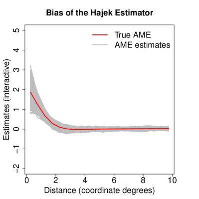
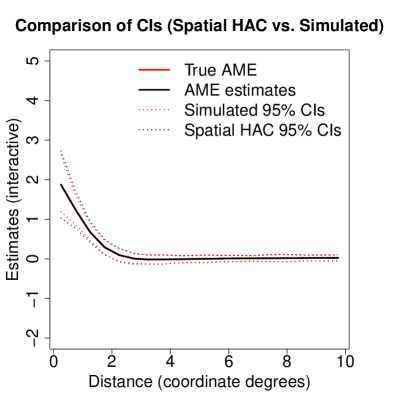
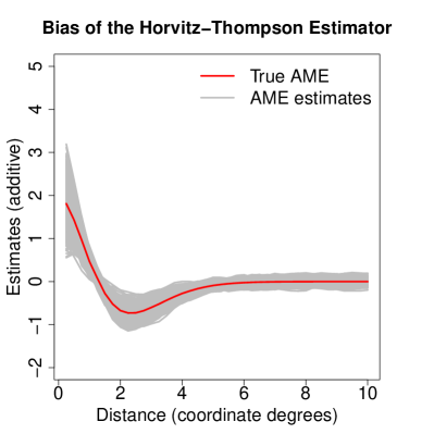
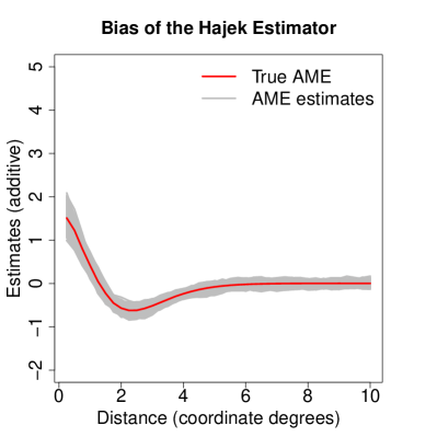
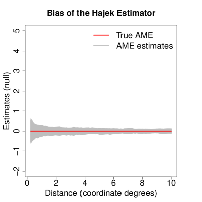
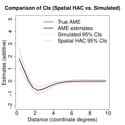
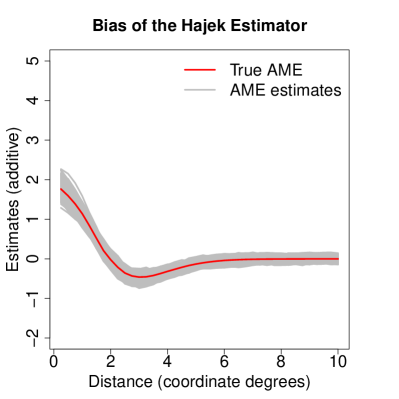
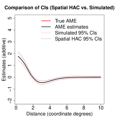
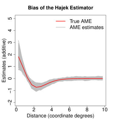
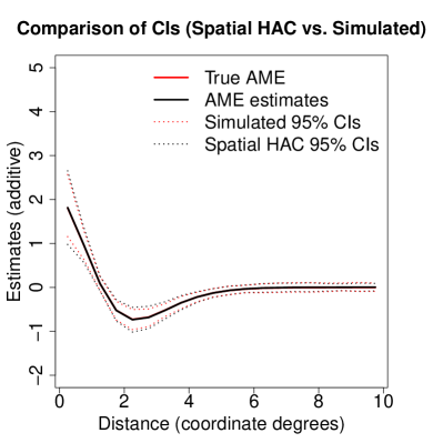
Figure 5 illustrates the bias of the proposed estimators. We can see from the left plots that the true AME curve resides in the middle of the Hajek estimates from repeated assignments, suggesting the estimator’s bias is indeed negligible even in finite samples. Plots on the right compare the average of the 95% confidence interval endpoints constructed from the spatial HAC standard errors with the simulated 95% confidence intervals (i.e., the 2.5% and 97.5% quantiles from the permutation distribution of the effect estimates) under both the additive and the interactive effect functions. It confirms our conclusion that the spatial HAC inference is valid but slightly conservative.101010Remember that the effect curves are smooth hence the assumption of homophily holds. As d𝑑d increases, the effect gradually diminishes hence the estimated standard errors equal the simulated standard errors.
Refer to caption
Refer to caption
Refer to caption
Refer to caption
Figure 5: The bias of the Hajek estimator and the 95% spatial HAC confidence intervals under the additive (top) and interactive (bottom) effect functions. The red curves on the left figures indicate the true AME curve and each grey curve represents the Hajek estimates under one random assignment. On the right, the red dotted curves are the simulated 95% confidence intervals (i.e., the 2.5% and 97.5% quantiles of the permutation distribution) and the black dotted curves are the averages of 95% spatial HAC confidence intervals.

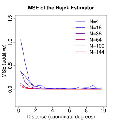
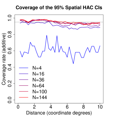
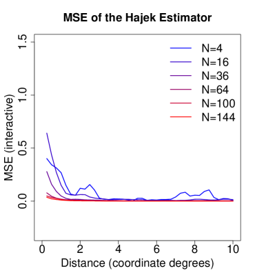
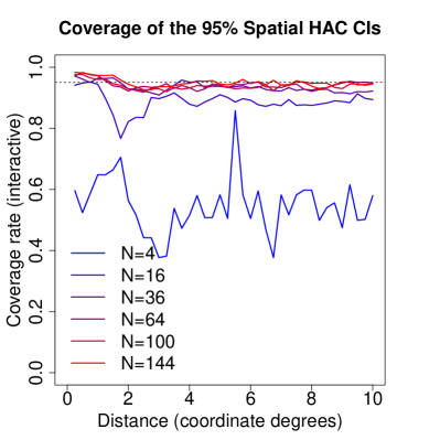
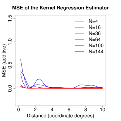
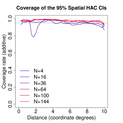
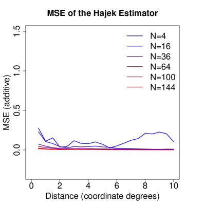
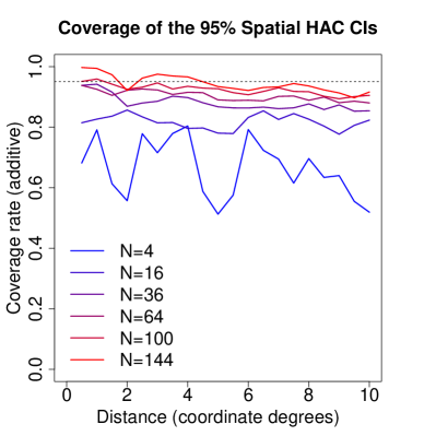
We present evidence on the proposed method’s asymptotic properties in Figure 6. Plots on the left show that the MSE of the AME estimator converges to zero at all distance values under both effect functions when the number of intervention nodes gradually rises (and the number of outcome points increases proportionally). Plots on the right show how coverage rates of the 95% confidence intervals generated by our approach vary across d𝑑d and N𝑁N. We can see that they are above the nominal rate of 95% when d𝑑d is small and converge near it at all distance values when N𝑁N is sufficiently large.

Refer to caption
Refer to caption
Refer to caption
Refer to caption
Figure 6: The top row is based on the additive effect function and the bottom one uses the interactive effect function. Each curve on the left plots shows the estimates’ mean squared error (MSE) at each distance given the sample size. Plots on the right how the average coverage rate of the 95% spatial HAC confidence interval at each distance changes with the sample size. Each curve represents the confidence interval’s average coverage rate at each distance value for a given sample size. The dotted horizontal line is the nominal coverage rate (95%).

8 Examples

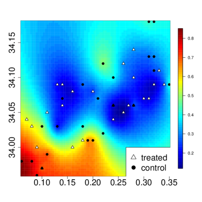
We demonstrate how to apply our methods in empirical studies using two examples. The first example is the study by Miguel and Kremer (2004) on the effects of a deworming intervention for youth in rural Kenya. In this study, pupils from 25 randomly picked schools out of 50 received deworming treatments. The left plot of Figure 7 shows the spatial distribution of treated and control schools. For the present analysis, we focus on the effect of the treatment on worms infection rates.111111The original study then went on to assess how reducing worms infections affected educational outcomes. The available data offer information on infection rates aggregated to the level of the schools. So to estimate how effects might vary over space, we used a kriging estimator to interpolate these infection rates over the entire raster surface. We then estimate the AME with these interpolated values, considering each school as an intervention node and each tile in the raster as an outcome point. Because these interpolated values vary smoothly, we calculate the circle averages using points on the edge of each circle. The range of distance values increases from 0 km to 40 km, with a step size of 1 km.

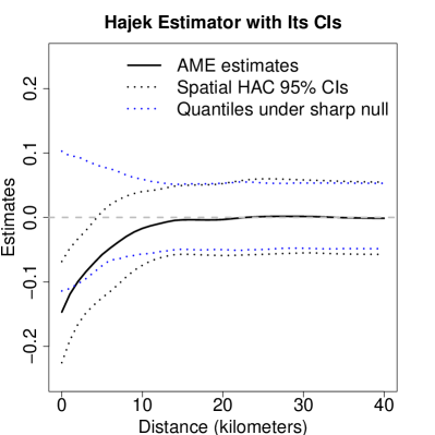
From the right plot of Figure 7, we can see that the estimated effects are significantly negative when d𝑑d is smaller than 2 km, whether judging from the permutation distribution under the sharp null or the spatial HAC confidence intervals. The result confirms the original finding of the paper that there exists a significant difference in infection prevalence between treated and untreated schools, even after accounting for the influence of interference. It also indicates a potentially beneficial effect diffusing outward in a small neighborhood around each intervention node. The threshold value we set for the spatial HAC variance estimator is 8 km.
Refer to caption
Refer to caption
Figure 7: The plot on the left demonstrates both the treatment status of each school and interpolated outcome values from kriging in the experiment. White triangles are schools under control and black circles are treated schools. The color on the map indicates the infection rate. The plot on the right presents results using our methods. The black curve represents the AME estimate. The AME is expressed in terms of effects on the infection rate at varying distances from the schools. The black curves are 95% confidence intervals constructed from spatial HAC standard errors. The blue lines are the 2.5% and 97.5% quantiles of the effect estimates under the sharp null.

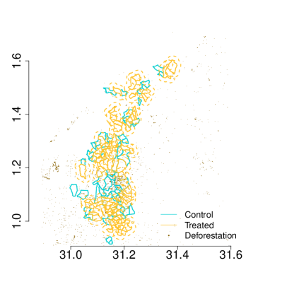
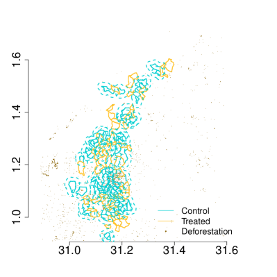
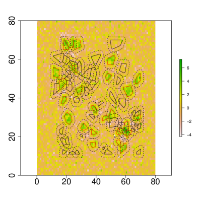
The second example is the forest conservation experiment from Jayachandran et al. (2017). The authors evaluate the effects of a “payments for ecosystems services” (PES) program based on 121 villages in Hoima and northern Kibaale districts of Uganda. 60 villages were randomly assigned to the treatment group. Private forest owners in these villages were paid to reduce deforestation on their own land over a course of two years, from 2011 to 2013. Figure 8 shows the location of each village in the experiment and its treatment status. We measure the outcome of interest using the forest cover dataset from Hansen et al. (2013) for years 2012 and 2013, and code Coveredx,t𝐶𝑜𝑣𝑒𝑟𝑒subscript𝑑𝑥𝑡Covered_{x,t} as 111 if raster tile x𝑥x’s forest coverage rate is greater than 25% in year t𝑡t, as 00 otherwise. We plot the distribution of ΔCoveredx=Coveredx,2013Coveredx,2012Δ𝐶𝑜𝑣𝑒𝑟𝑒subscript𝑑𝑥𝐶𝑜𝑣𝑒𝑟𝑒subscript𝑑𝑥2013𝐶𝑜𝑣𝑒𝑟𝑒subscript𝑑𝑥2012\Delta Covered_{x}=Covered_{x,2013}-Covered_{x,2012} in Figure 8. Dark spots on the map indicate where deforestation happened, that is, ΔCoveredx=1Δ𝐶𝑜𝑣𝑒𝑟𝑒subscript𝑑𝑥1\Delta Covered_{x}=1.

Refer to caption
Refer to caption
Figure 8: Both plots show the boundary of the 121 villages in Jayachandran et al. (2017). Villages with a golden boundary are treated and those with a turquoise boundary are under control. Dark spots on the map represent deforestation during the experiment. The left plot shows buffers around each treated village and the right one shows buffers around each untreated village.

The original analysis in the paper focuses on ΔCoveredxΔ𝐶𝑜𝑣𝑒𝑟𝑒subscript𝑑𝑥\Delta Covered_{x} within the boundary of the villages. We are interested in whether ΔCoveredxΔ𝐶𝑜𝑣𝑒𝑟𝑒subscript𝑑𝑥\Delta Covered_{x} outside the villages is reduced by the intervention. We consider the villages as polygons rather than points due to their relative sizes on the geography. To construct the circle averages, we generate buffers around each of the villages. For each point on a buffer, its minimal distance to the polygon in the center is the same number d𝑑d, the radius of the buffer. We then take the average over all the points between two buffers (a “donut”) rather than over those on the edge of each buffer. Hence, the distance value 00 refers to the area within the boundary of the villages. To facilitate the analysis, we re-project the data onto a plane and use the Euclidean distance. The distance range is set to be between 0 km and 20 km and the threshold value is 5 km.
Refer to caption Refer to caption

Refer to caption Refer to caption

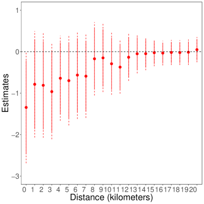
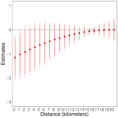
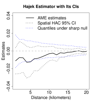
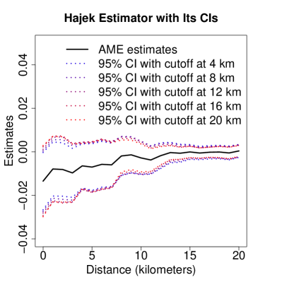
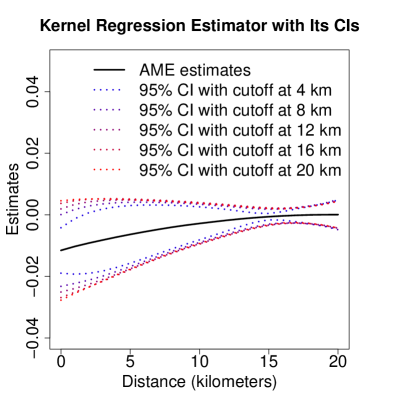
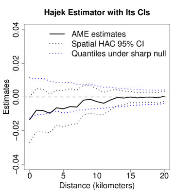
Figure 9: Plots on the left present results from the Hajek estimator, while plots on the right present those from the kernel regression estimator. On the top, the effects and their 95% confidence intervals are shown as curves. The black solid line represents the estimated AME at each distance value. The black dotted lines around it are the 95% spatial HAC confidence intervals. The blue dotted lines are the 2.5% and 97.5% quantiles of the effect estimates under the sharp null. On the bottom are coefficients plots. The solid segments mark the 95% spatial HAC confidence intervals and the dotted ones mark the 90% spatial HAC confidence intervals.

In Figure 9, plots on the left report results from the Hajek estimator, and plots on the right report results from the kernel regression estimator. On the top, we show the AME estimates and their 95% confidence intervals as curves. On the bottom, we present them as coefficient estimates. Both estimators detect a significant decrease of deforestation within the boundary of the villages, even though the magnitude is smaller than what the authors reported.121212A possible reason is that the data the authors used came from a commercial satellite company, which has a higher resolution than ours. We also find evidence of spillover effects in space. It is harder to tell from the Hajek estimates as their values are more jagged across distance values. But from the estimates generated by the kernel regression estimator, we can see that the effect is significant at the 10% level for areas which within 2 km of the boundary of the treated villages. Our permutation test confirms the conclusion. We show in the appendix that the results are robust to a range of threshold values.

9 Conclusion

When treatments are applied at given intervention nodes in space, the effects may bleed out in complex ways. Moreover, effects that bleed out from multiple nodes may interact with each other. As a result, the spatial effects at any point can depend on the entire distribution of treatments over intervention nodes, rather than on the treatment status of only the nearest node. To capture such effects adequately, one needs to account for such interference appropriately. Standard approaches, which ignore such interference, yield conclusions about average policy impacts that may be unwarranted.

This paper explains how one can account for such interference in a randomized spatial experiment and estimate a meaningful spatial effect—what we call the “average marginalized effect” (AME). The AME tells us what would happen, on average, if we switch an intervention node at a given distance into treatment, averaging over ambient effects emanating from other intervention nodes. We can construct AME estimates for difference distances, yielding a spatial effect curve. The AME is identified under random assignment as a simple contrast. Under restrictions on the spatial extent of interference, we can estimate the AME consistently and perform accurate inference using simple difference-in-means estimators and readily-available spatial standard error estimators.

We also develop a number of extensions. This includes the specification of conditions under which the AME can be interpreted as a structural quantity that does not depend on the experimental design. We offer an approach for potentially increasing statistical power by allowing for smoothing over distance, and explain how to test hypotheses on joint effects using Fisher-style permutation under the sharp null.

We illustrate our approach using simulation and two examples from real-world spatial experiments. The examples show the soundness of our proposed methods but also point to areas for refinement in further research. These include introducing methods to boost power, for example, by incorporating spatial covariate information, and to further improve finite sample inference.

Appendix A Analytical results

We first prove the unbiasedness of the Horvitz-Thompson estimator for the AME. We then characterize the variance of the Horvitz-Thompson estimator and the Hajek estimator, as well as their rates of convergence. We put all of these pieces together to prove the results for asymptotic distributions. Finally, we show that the regression-based approach using the spatial HAC standard errors provides for conservative inference.

A.1 Lemmas

We first state a lemma for the analysis that follows.

Lemma A.1.

For any function f:{0,1}N:𝑓superscript01𝑁f:\{0,1\}^{N}\to\mathbb{R}, assuming C1𝐶1C\ref{assn:bern-des}, we have:

C1.1

E[Zikf(𝐙)]=pE𝐙i[f(1,𝐙i)]Edelimited-[]superscriptsubscript𝑍𝑖𝑘𝑓𝐙𝑝subscriptEsubscript𝐙𝑖delimited-[]𝑓1subscript𝐙𝑖{\rm E}\,\left[Z_{i}^{k}f(\mathbf{Z})\right]=p{\rm E}\,_{\mathbf{Z}_{-i}}\left[f(1,\mathbf{Z}_{-i})\right] for any integer k𝑘k131313Without further notification, the expectation is always taken over 𝐙𝐙\mathbf{Z} in what follows..

C1.2

E[ZikZjlf(𝐙)]=p2E𝐙(i,j)[f(1,1,𝐙(i,j))]Edelimited-[]superscriptsubscript𝑍𝑖𝑘superscriptsubscript𝑍𝑗𝑙𝑓𝐙superscript𝑝2subscriptEsubscript𝐙𝑖𝑗delimited-[]𝑓11subscript𝐙𝑖𝑗{\rm E}\,\left[Z_{i}^{k}Z_{j}^{l}f(\mathbf{Z})\right]=p^{2}{\rm E}\,_{\mathbf{Z}_{-(i,j)}}\left[f(1,1,\mathbf{Z}_{-(i,j)})\right] for any integer k𝑘k and l𝑙l.

Proof.

By Law of Iterated Expectations. ∎

A.2 Proposition 1 (Horvitz-Thompson Unbiasedness)

Proof.

Recall the definition of the Horvitz-Thompson estimator in (1): τ^(d)=1Npi=1NZiμi(𝐘;d)1N(1p)i=1N(1Zi)μi(𝐘;d)^𝜏𝑑1𝑁𝑝superscriptsubscript𝑖1𝑁subscript𝑍𝑖subscript𝜇𝑖𝐘𝑑1𝑁1𝑝superscriptsubscript𝑖1𝑁1subscript𝑍𝑖subscript𝜇𝑖𝐘𝑑\widehat{\tau}(d)=\frac{1}{Np}\sum_{i=1}^{N}Z_{i}\mu_{i}(\mathbf{Y};d)-\frac{1}{N(1-p)}\sum_{i=1}^{N}(1-Z_{i})\mu_{i}(\mathbf{Y};d).

τ(d;η)𝜏𝑑𝜂\displaystyle\tau(d;\eta) =1Ni=1Nμi(1;d,η)1Ni=1Nμi(0;d,η)absent1𝑁superscriptsubscript𝑖1𝑁subscript𝜇𝑖1𝑑𝜂1𝑁superscriptsubscript𝑖1𝑁subscript𝜇𝑖0𝑑𝜂\displaystyle=\frac{1}{N}\sum_{i=1}^{N}\mu_{i}(1;d,\eta)-\frac{1}{N}\sum_{i=1}^{N}\mu_{i}(0;d,\eta)
=1Npi=1NpE𝐙i[μi(𝐘(1,𝐙i);d)]1N(1p)i=1N(1p)E𝐙i[μi(𝐘(0,𝐙i);d)]absent1𝑁𝑝superscriptsubscript𝑖1𝑁𝑝subscriptEsubscript𝐙𝑖delimited-[]subscript𝜇𝑖𝐘1subscript𝐙𝑖𝑑1𝑁1𝑝superscriptsubscript𝑖1𝑁1𝑝subscriptEsubscript𝐙𝑖delimited-[]subscript𝜇𝑖𝐘0subscript𝐙𝑖𝑑\displaystyle=\frac{1}{Np}\sum_{i=1}^{N}p{\rm E}\,_{\mathbf{Z}_{-i}}[\mu_{i}(\mathbf{Y}(1,\mathbf{Z}_{-i});d)]-\frac{1}{N(1-p)}\sum_{i=1}^{N}(1-p){\rm E}\,_{\mathbf{Z}_{-i}}[\mu_{i}(\mathbf{Y}(0,\mathbf{Z}_{-i});d)]
=1Npi=1NE𝐙[Ziμi(𝐘;d)]1N(1p)i=1NE𝐙[(1Zi)μi(𝐘;d)]absent1𝑁𝑝superscriptsubscript𝑖1𝑁subscriptE𝐙delimited-[]subscript𝑍𝑖subscript𝜇𝑖𝐘𝑑1𝑁1𝑝superscriptsubscript𝑖1𝑁subscriptE𝐙delimited-[]1subscript𝑍𝑖subscript𝜇𝑖𝐘𝑑\displaystyle=\frac{1}{Np}\sum_{i=1}^{N}{\rm E}\,_{\mathbf{Z}}[Z_{i}\mu_{i}(\mathbf{Y};d)]-\frac{1}{N(1-p)}\sum_{i=1}^{N}{\rm E}\,_{\mathbf{Z}}[(1-Z_{i})\mu_{i}(\mathbf{Y};d)]
=E𝐙[1Npi=1NZiμi(𝐘;d)1N(1p)i=1N(1Zi)μi(𝐘;d)],absentsubscriptE𝐙delimited-[]1𝑁𝑝superscriptsubscript𝑖1𝑁subscript𝑍𝑖subscript𝜇𝑖𝐘𝑑1𝑁1𝑝superscriptsubscript𝑖1𝑁1subscript𝑍𝑖subscript𝜇𝑖𝐘𝑑\displaystyle={\rm E}\,_{\mathbf{Z}}\left[\frac{1}{Np}\sum_{i=1}^{N}Z_{i}\mu_{i}(\mathbf{Y};d)-\frac{1}{N(1-p)}\sum_{i=1}^{N}(1-Z_{i})\mu_{i}(\mathbf{Y};d)\right],

where the second equality uses the definition of μi(z;d,η)subscript𝜇𝑖𝑧𝑑𝜂\mu_{i}(z;d,\eta), the third equality follows from Lemma A.1. ∎

We now characterize the variance of the Horvitz-Thompson estimator.

Lemma A.2.

Under conditions C1-C3 as defined in the main text, the variance of estimator τ^(d)^𝜏𝑑\widehat{\tau}(d) is bounded as follows:

Var(τ^(d))Var^𝜏𝑑\displaystyle{\rm Var}\,\left(\widehat{\tau}(d)\right)
\displaystyle\leq 1N2pi=1NE[μi2(𝐘(1,𝐙i);d)]+1N2(1p)i=1NE[μi2(𝐘(0,𝐙i);d)]1superscript𝑁2𝑝superscriptsubscript𝑖1𝑁Edelimited-[]superscriptsubscript𝜇𝑖2𝐘1subscript𝐙𝑖𝑑1superscript𝑁21𝑝superscriptsubscript𝑖1𝑁Edelimited-[]superscriptsubscript𝜇𝑖2𝐘0subscript𝐙𝑖𝑑\displaystyle\frac{1}{N^{2}p}\sum_{i=1}^{N}{\rm E}\,\left[\mu_{i}^{2}(\mathbf{Y}(1,\mathbf{Z}_{-i});d)\right]+\frac{1}{N^{2}(1-p)}\sum_{i=1}^{N}{\rm E}\,\left[\mu_{i}^{2}(\mathbf{Y}(0,\mathbf{Z}_{-i});d)\right]
+1N2i=1Nj(i;d)a,b=01(1)a+b{E[μi(𝐘(a,b,𝐙(i,j));d)μj(𝐘(a,b,𝐙(i,j));d)]\displaystyle+\frac{1}{N^{2}}\sum_{i=1}^{N}\sum_{j\in\mathcal{B}(i;d)}\sum_{a,b=0}^{1}(-1)^{a+b}\Big{\{}{\rm E}\,\left[\mu_{i}(\mathbf{Y}(a,b,\mathbf{Z}_{-(i,j)});d)\mu_{j}(\mathbf{Y}(a,b,\mathbf{Z}_{-(i,j)});d)\right]
E[μi(𝐘(a,𝐙i);d)]E[μj(𝐘(b,𝐙j);d)]},\displaystyle-{\rm E}\,\left[\mu_{i}(\mathbf{Y}(a,\mathbf{Z}_{-i});d)\right]{\rm E}\,\left[\mu_{j}(\mathbf{Y}(b,\mathbf{Z}_{-j});d)\right]\Big{\}},

and we have that

Var(τ^(d))=O(1N).Var^𝜏𝑑𝑂1𝑁\displaystyle{\rm Var}\,\left(\widehat{\tau}(d)\right)=O\left(\frac{1}{N}\right).
Proof.

Using the expression of the Horvitz-Thompson estimator, we have:

Var(τ^(d))Var^𝜏𝑑\displaystyle{\rm Var}\,\left(\widehat{\tau}(d)\right)
=\displaystyle= 1N2Var[i=1N(Zip1Zi1p)μi(𝐘(𝐙);d)]1superscript𝑁2Vardelimited-[]superscriptsubscript𝑖1𝑁subscript𝑍𝑖𝑝1subscript𝑍𝑖1𝑝subscript𝜇𝑖𝐘𝐙𝑑\displaystyle\frac{1}{N^{2}}{\rm Var}\,\left[\sum_{i=1}^{N}\left(\frac{Z_{i}}{p}-\frac{1-Z_{i}}{1-p}\right)\mu_{i}(\mathbf{Y}(\mathbf{Z});d)\right]
=\displaystyle= 1N2i=1NVar[(Zip1Zi1p)μi(𝐘(𝐙);d)]1superscript𝑁2superscriptsubscript𝑖1𝑁Vardelimited-[]subscript𝑍𝑖𝑝1subscript𝑍𝑖1𝑝subscript𝜇𝑖𝐘𝐙𝑑\displaystyle\frac{1}{N^{2}}\sum_{i=1}^{N}{\rm Var}\,\left[\left(\frac{Z_{i}}{p}-\frac{1-Z_{i}}{1-p}\right)\mu_{i}(\mathbf{Y}(\mathbf{Z});d)\right]
+1N2i=1NjiCov[(Zip1Zi1p)μi(𝐘(𝐙);d),(Zjp1Zj1p)μj(𝐘(𝐙);d)]1superscript𝑁2superscriptsubscript𝑖1𝑁subscript𝑗𝑖Covsubscript𝑍𝑖𝑝1subscript𝑍𝑖1𝑝subscript𝜇𝑖𝐘𝐙𝑑subscript𝑍𝑗𝑝1subscript𝑍𝑗1𝑝subscript𝜇𝑗𝐘𝐙𝑑\displaystyle+\frac{1}{N^{2}}\sum_{i=1}^{N}\sum_{j\neq i}{\rm Cov}\,\left[\left(\frac{Z_{i}}{p}-\frac{1-Z_{i}}{1-p}\right)\mu_{i}(\mathbf{Y}(\mathbf{Z});d),\left(\frac{Z_{j}}{p}-\frac{1-Z_{j}}{1-p}\right)\mu_{j}(\mathbf{Y}(\mathbf{Z});d)\right]
=\displaystyle= 1N2i=1NE[((Zip1Zi1p)μi(𝐘(𝐙);d))2]1N2i=1N(E[(Zip1Zi1p)μi(𝐘(𝐙);d)])21superscript𝑁2superscriptsubscript𝑖1𝑁Edelimited-[]superscriptsubscript𝑍𝑖𝑝1subscript𝑍𝑖1𝑝subscript𝜇𝑖𝐘𝐙𝑑21superscript𝑁2superscriptsubscript𝑖1𝑁superscriptEdelimited-[]subscript𝑍𝑖𝑝1subscript𝑍𝑖1𝑝subscript𝜇𝑖𝐘𝐙𝑑2\displaystyle\frac{1}{N^{2}}\sum_{i=1}^{N}{\rm E}\,\left[\left(\left(\frac{Z_{i}}{p}-\frac{1-Z_{i}}{1-p}\right)\mu_{i}(\mathbf{Y}(\mathbf{Z});d)\right)^{2}\right]-\frac{1}{N^{2}}\sum_{i=1}^{N}\left({\rm E}\,\left[\left(\frac{Z_{i}}{p}-\frac{1-Z_{i}}{1-p}\right)\mu_{i}(\mathbf{Y}(\mathbf{Z});d)\right]\right)^{2}
+1N2i=1NjiCov[Zipμi(𝐘(𝐙);d),Zjpμj(𝐘(𝐙);d)]1superscript𝑁2superscriptsubscript𝑖1𝑁subscript𝑗𝑖Covsubscript𝑍𝑖𝑝subscript𝜇𝑖𝐘𝐙𝑑subscript𝑍𝑗𝑝subscript𝜇𝑗𝐘𝐙𝑑\displaystyle+\frac{1}{N^{2}}\sum_{i=1}^{N}\sum_{j\neq i}{\rm Cov}\,\left[\frac{Z_{i}}{p}\mu_{i}(\mathbf{Y}(\mathbf{Z});d),\frac{Z_{j}}{p}\mu_{j}(\mathbf{Y}(\mathbf{Z});d)\right]
1N2i=1NjiCov[Zipμi(𝐘(𝐙);d),1Zj1pμj(𝐘(𝐙);d)]1superscript𝑁2superscriptsubscript𝑖1𝑁subscript𝑗𝑖Covsubscript𝑍𝑖𝑝subscript𝜇𝑖𝐘𝐙𝑑1subscript𝑍𝑗1𝑝subscript𝜇𝑗𝐘𝐙𝑑\displaystyle-\frac{1}{N^{2}}\sum_{i=1}^{N}\sum_{j\neq i}{\rm Cov}\,\left[\frac{Z_{i}}{p}\mu_{i}(\mathbf{Y}(\mathbf{Z});d),\frac{1-Z_{j}}{1-p}\mu_{j}(\mathbf{Y}(\mathbf{Z});d)\right]
1N2i=1NjiCov[1Zi1pμi(𝐘(𝐙);d),Zjpμj(𝐘(𝐙);d)]1superscript𝑁2superscriptsubscript𝑖1𝑁subscript𝑗𝑖Cov1subscript𝑍𝑖1𝑝subscript𝜇𝑖𝐘𝐙𝑑subscript𝑍𝑗𝑝subscript𝜇𝑗𝐘𝐙𝑑\displaystyle-\frac{1}{N^{2}}\sum_{i=1}^{N}\sum_{j\neq i}{\rm Cov}\,\left[\frac{1-Z_{i}}{1-p}\mu_{i}(\mathbf{Y}(\mathbf{Z});d),\frac{Z_{j}}{p}\mu_{j}(\mathbf{Y}(\mathbf{Z});d)\right]
+1N2i=1NjiCov[1Zi1pμi(𝐘(𝐙);d),1Zj1pμj(𝐘(𝐙);d)].1superscript𝑁2superscriptsubscript𝑖1𝑁subscript𝑗𝑖Cov1subscript𝑍𝑖1𝑝subscript𝜇𝑖𝐘𝐙𝑑1subscript𝑍𝑗1𝑝subscript𝜇𝑗𝐘𝐙𝑑\displaystyle+\frac{1}{N^{2}}\sum_{i=1}^{N}\sum_{j\neq i}{\rm Cov}\,\left[\frac{1-Z_{i}}{1-p}\mu_{i}(\mathbf{Y}(\mathbf{Z});d),\frac{1-Z_{j}}{1-p}\mu_{j}(\mathbf{Y}(\mathbf{Z});d)\right].

We further expand the first two terms in the above expression:

1N2i=1NE[((Zip1Zi1p)μi(𝐘(𝐙);d))2]1N2i=1NE[(Zip1Zi1p)μi(𝐘(𝐙);d)]21superscript𝑁2superscriptsubscript𝑖1𝑁Edelimited-[]superscriptsubscript𝑍𝑖𝑝1subscript𝑍𝑖1𝑝subscript𝜇𝑖𝐘𝐙𝑑21superscript𝑁2superscriptsubscript𝑖1𝑁Esuperscriptdelimited-[]subscript𝑍𝑖𝑝1subscript𝑍𝑖1𝑝subscript𝜇𝑖𝐘𝐙𝑑2\displaystyle\frac{1}{N^{2}}\sum_{i=1}^{N}{\rm E}\,\left[\left(\left(\frac{Z_{i}}{p}-\frac{1-Z_{i}}{1-p}\right)\mu_{i}(\mathbf{Y}(\mathbf{Z});d)\right)^{2}\right]-\frac{1}{N^{2}}\sum_{i=1}^{N}{\rm E}\,\left[\left(\frac{Z_{i}}{p}-\frac{1-Z_{i}}{1-p}\right)\mu_{i}(\mathbf{Y}(\mathbf{Z});d)\right]^{2}
=\displaystyle= 1N2i=1NE[Zi2p2μi2(𝐘(𝐙);d)]+1N2i=1NE[(1Zi)2(1p)2μi2(𝐘(𝐙);d)]1superscript𝑁2superscriptsubscript𝑖1𝑁Edelimited-[]superscriptsubscript𝑍𝑖2superscript𝑝2superscriptsubscript𝜇𝑖2𝐘𝐙𝑑1superscript𝑁2superscriptsubscript𝑖1𝑁Edelimited-[]superscript1subscript𝑍𝑖2superscript1𝑝2superscriptsubscript𝜇𝑖2𝐘𝐙𝑑\displaystyle\frac{1}{N^{2}}\sum_{i=1}^{N}{\rm E}\,\left[\frac{Z_{i}^{2}}{p^{2}}\mu_{i}^{2}(\mathbf{Y}(\mathbf{Z});d)\right]+\frac{1}{N^{2}}\sum_{i=1}^{N}{\rm E}\,\left[\frac{(1-Z_{i})^{2}}{(1-p)^{2}}\mu_{i}^{2}(\mathbf{Y}(\mathbf{Z});d)\right]
1N2i=1NE2[(Zip1Zi1p)μi(𝐘(𝐙);d)]1superscript𝑁2superscriptsubscript𝑖1𝑁superscriptE2delimited-[]subscript𝑍𝑖𝑝1subscript𝑍𝑖1𝑝subscript𝜇𝑖𝐘𝐙𝑑\displaystyle-\frac{1}{N^{2}}\sum_{i=1}^{N}{\rm E}\,^{2}\left[\left(\frac{Z_{i}}{p}-\frac{1-Z_{i}}{1-p}\right)\mu_{i}(\mathbf{Y}(\mathbf{Z});d)\right]
=\displaystyle= 1N2pi=1NE[μi2(𝐘(1,𝐙i);d)]+1N2(1p)i=1NE[μi2(𝐘(0,𝐙i);d)]1superscript𝑁2𝑝superscriptsubscript𝑖1𝑁Edelimited-[]superscriptsubscript𝜇𝑖2𝐘1subscript𝐙𝑖𝑑1superscript𝑁21𝑝superscriptsubscript𝑖1𝑁Edelimited-[]superscriptsubscript𝜇𝑖2𝐘0subscript𝐙𝑖𝑑\displaystyle\frac{1}{N^{2}p}\sum_{i=1}^{N}{\rm E}\,\left[\mu_{i}^{2}(\mathbf{Y}(1,\mathbf{Z}_{-i});d)\right]+\frac{1}{N^{2}(1-p)}\sum_{i=1}^{N}{\rm E}\,\left[\mu_{i}^{2}(\mathbf{Y}(0,\mathbf{Z}_{-i});d)\right]
1N2i=1NE2[μi(𝐘(1,𝐙i);d)μi(𝐘(0,𝐙i);d)]1superscript𝑁2superscriptsubscript𝑖1𝑁superscriptE2delimited-[]subscript𝜇𝑖𝐘1subscript𝐙𝑖𝑑subscript𝜇𝑖𝐘0subscript𝐙𝑖𝑑\displaystyle-\frac{1}{N^{2}}\sum_{i=1}^{N}{\rm E}\,^{2}\left[\mu_{i}(\mathbf{Y}(1,\mathbf{Z}_{-i});d)-\mu_{i}(\mathbf{Y}(0,\mathbf{Z}_{-i});d)\right]
\displaystyle\leq 1N2pi=1NE[μi2(𝐘(1,𝐙i);d)]+1N2(1p)i=1NE[μi2(𝐘(0,𝐙i);d)].1superscript𝑁2𝑝superscriptsubscript𝑖1𝑁Edelimited-[]superscriptsubscript𝜇𝑖2𝐘1subscript𝐙𝑖𝑑1superscript𝑁21𝑝superscriptsubscript𝑖1𝑁Edelimited-[]superscriptsubscript𝜇𝑖2𝐘0subscript𝐙𝑖𝑑\displaystyle\frac{1}{N^{2}p}\sum_{i=1}^{N}{\rm E}\,\left[\mu_{i}^{2}(\mathbf{Y}(1,\mathbf{Z}_{-i});d)\right]+\frac{1}{N^{2}(1-p)}\sum_{i=1}^{N}{\rm E}\,\left[\mu_{i}^{2}(\mathbf{Y}(0,\mathbf{Z}_{-i});d)\right].

We also have:

1Npi=1NE[μi2(𝐘(1,𝐙i);d)]+1N(1p)i=1NE[μi2(𝐘(0,𝐙i);d)]1𝑁𝑝superscriptsubscript𝑖1𝑁Edelimited-[]superscriptsubscript𝜇𝑖2𝐘1subscript𝐙𝑖𝑑1𝑁1𝑝superscriptsubscript𝑖1𝑁Edelimited-[]superscriptsubscript𝜇𝑖2𝐘0subscript𝐙𝑖𝑑\displaystyle\frac{1}{Np}\sum_{i=1}^{N}{\rm E}\,\left[\mu_{i}^{2}(\mathbf{Y}(1,\mathbf{Z}_{-i});d)\right]+\frac{1}{N(1-p)}\sum_{i=1}^{N}{\rm E}\,\left[\mu_{i}^{2}(\mathbf{Y}(0,\mathbf{Z}_{-i});d)\right]
1Ni=1NE2[μi(𝐘(1,𝐙i);d)μi(𝐘(0,𝐙i);d)]=O(1),1𝑁superscriptsubscript𝑖1𝑁superscriptE2delimited-[]subscript𝜇𝑖𝐘1subscript𝐙𝑖𝑑subscript𝜇𝑖𝐘0subscript𝐙𝑖𝑑𝑂1\displaystyle-\frac{1}{N}\sum_{i=1}^{N}{\rm E}\,^{2}\left[\mu_{i}(\mathbf{Y}(1,\mathbf{Z}_{-i});d)-\mu_{i}(\mathbf{Y}(0,\mathbf{Z}_{-i});d)\right]=O\left(1\right),

since C2 implies that all the moments are bounded. Next, we examine the first covariance term, which equals

1N2i=1NjiCov[Zipμi(𝐘(𝐙);d),Zjpμj(𝐘(𝐙);d)]1superscript𝑁2superscriptsubscript𝑖1𝑁subscript𝑗𝑖Covsubscript𝑍𝑖𝑝subscript𝜇𝑖𝐘𝐙𝑑subscript𝑍𝑗𝑝subscript𝜇𝑗𝐘𝐙𝑑\displaystyle\frac{1}{N^{2}}\sum_{i=1}^{N}\sum_{j\neq i}{\rm Cov}\,\left[\frac{Z_{i}}{p}\mu_{i}(\mathbf{Y}(\mathbf{Z});d),\frac{Z_{j}}{p}\mu_{j}(\mathbf{Y}(\mathbf{Z});d)\right]
=\displaystyle= 1N2i=1NjiE[ZiZjp2μi(𝐘(𝐙);d)μj(𝐘(𝐙);d)]1superscript𝑁2superscriptsubscript𝑖1𝑁subscript𝑗𝑖Edelimited-[]subscript𝑍𝑖subscript𝑍𝑗superscript𝑝2subscript𝜇𝑖𝐘𝐙𝑑subscript𝜇𝑗𝐘𝐙𝑑\displaystyle\frac{1}{N^{2}}\sum_{i=1}^{N}\sum_{j\neq i}{\rm E}\,\left[\frac{Z_{i}Z_{j}}{p^{2}}\mu_{i}(\mathbf{Y}(\mathbf{Z});d)\mu_{j}(\mathbf{Y}(\mathbf{Z});d)\right]
1N2i=1NjiE[Zipμi(𝐘(𝐙);d)]E[Zjpμj(𝐘(𝐙);d)]1superscript𝑁2superscriptsubscript𝑖1𝑁subscript𝑗𝑖Edelimited-[]subscript𝑍𝑖𝑝subscript𝜇𝑖𝐘𝐙𝑑Edelimited-[]subscript𝑍𝑗𝑝subscript𝜇𝑗𝐘𝐙𝑑\displaystyle-\frac{1}{N^{2}}\sum_{i=1}^{N}\sum_{j\neq i}{\rm E}\,\left[\frac{Z_{i}}{p}\mu_{i}(\mathbf{Y}(\mathbf{Z});d)\right]{\rm E}\,\left[\frac{Z_{j}}{p}\mu_{j}(\mathbf{Y}(\mathbf{Z});d)\right]
=\displaystyle= 1N2i=1NjiE[μi(𝐘(1,1,𝐙(i,j));d)μj(𝐘(1,1,𝐙(i,j));d)]1superscript𝑁2superscriptsubscript𝑖1𝑁subscript𝑗𝑖Edelimited-[]subscript𝜇𝑖𝐘11subscript𝐙𝑖𝑗𝑑subscript𝜇𝑗𝐘11subscript𝐙𝑖𝑗𝑑\displaystyle\frac{1}{N^{2}}\sum_{i=1}^{N}\sum_{j\neq i}{\rm E}\,\left[\mu_{i}(\mathbf{Y}(1,1,\mathbf{Z}_{-(i,j)});d)\mu_{j}(\mathbf{Y}(1,1,\mathbf{Z}_{-(i,j)});d)\right]
1N2i=1NjiE[μi(𝐘(1,𝐙i);d)]E[μj(𝐘(1,𝐙i);d)]1superscript𝑁2superscriptsubscript𝑖1𝑁subscript𝑗𝑖Edelimited-[]subscript𝜇𝑖𝐘1subscript𝐙𝑖𝑑Edelimited-[]subscript𝜇𝑗𝐘1subscript𝐙𝑖𝑑\displaystyle-\frac{1}{N^{2}}\sum_{i=1}^{N}\sum_{j\neq i}{\rm E}\,\left[\mu_{i}(\mathbf{Y}(1,\mathbf{Z}_{-i});d)\right]{\rm E}\,\left[\mu_{j}(\mathbf{Y}(1,\mathbf{Z}_{-i});d)\right]
=\displaystyle= 1N2i=1Nj(i;d)E[μi(𝐘(1,1,𝐙(i,j));d)μj(𝐘(1,1,𝐙(i,j));d)]1superscript𝑁2superscriptsubscript𝑖1𝑁subscript𝑗𝑖𝑑Edelimited-[]subscript𝜇𝑖𝐘11subscript𝐙𝑖𝑗𝑑subscript𝜇𝑗𝐘11subscript𝐙𝑖𝑗𝑑\displaystyle\frac{1}{N^{2}}\sum_{i=1}^{N}\sum_{j\in\mathcal{B}(i;d)}{\rm E}\,\left[\mu_{i}(\mathbf{Y}(1,1,\mathbf{Z}_{-(i,j)});d)\mu_{j}(\mathbf{Y}(1,1,\mathbf{Z}_{-(i,j)});d)\right]
1N2i=1Nj(i;d)E[μi(𝐘(1,𝐙i);d)]E[μj(𝐘(1,𝐙i);d)].1superscript𝑁2superscriptsubscript𝑖1𝑁subscript𝑗𝑖𝑑Edelimited-[]subscript𝜇𝑖𝐘1subscript𝐙𝑖𝑑Edelimited-[]subscript𝜇𝑗𝐘1subscript𝐙𝑖𝑑\displaystyle-\frac{1}{N^{2}}\sum_{i=1}^{N}\sum_{j\in\mathcal{B}(i;d)}{\rm E}\,\left[\mu_{i}(\mathbf{Y}(1,\mathbf{Z}_{-i});d)\right]{\rm E}\,\left[\mu_{j}(\mathbf{Y}(1,\mathbf{Z}_{-i});d)\right].

The last equality holds because of assumption C3 on local interference. For j(i)𝑗𝑖j\notin\mathcal{B}(i), μi(𝐘(1,1,𝐙(i,j));d)=μi(𝐘(1,𝐙i);d)subscript𝜇𝑖𝐘11subscript𝐙𝑖𝑗𝑑subscript𝜇𝑖𝐘1subscript𝐙𝑖𝑑\mu_{i}(\mathbf{Y}(1,1,\mathbf{Z}_{-(i,j)});d)=\mu_{i}(\mathbf{Y}(1,\mathbf{Z}_{-i});d) and E[μi(𝐘(1,1,𝐙(i,j));d)μj(𝐘(1,1,𝐙(i,j));d)]=E[μi(𝐘(1,1,𝐙(i,j));d)]E[μj(𝐘(1,1,𝐙(i,j));d)]Edelimited-[]subscript𝜇𝑖𝐘11subscript𝐙𝑖𝑗𝑑subscript𝜇𝑗𝐘11subscript𝐙𝑖𝑗𝑑Edelimited-[]subscript𝜇𝑖𝐘11subscript𝐙𝑖𝑗𝑑Edelimited-[]subscript𝜇𝑗𝐘11subscript𝐙𝑖𝑗𝑑{\rm E}\,\left[\mu_{i}(\mathbf{Y}(1,1,\mathbf{Z}_{-(i,j)});d)\mu_{j}(\mathbf{Y}(1,1,\mathbf{Z}_{-(i,j)});d)\right]={\rm E}\,\left[\mu_{i}(\mathbf{Y}(1,1,\mathbf{Z}_{-(i,j)});d)\right]{\rm E}\,\left[\mu_{j}(\mathbf{Y}(1,1,\mathbf{Z}_{-(i,j)});d)\right], following the definition of interference in Section 4. Moreover,

1Ni=1Nj(i;d)E[μi(𝐘(1,1,𝐙(i,j));d)μj(𝐘(1,1,𝐙(i,j));d)]1𝑁superscriptsubscript𝑖1𝑁subscript𝑗𝑖𝑑Edelimited-[]subscript𝜇𝑖𝐘11subscript𝐙𝑖𝑗𝑑subscript𝜇𝑗𝐘11subscript𝐙𝑖𝑗𝑑\displaystyle\frac{1}{N}\sum_{i=1}^{N}\sum_{j\in\mathcal{B}(i;d)}{\rm E}\,\left[\mu_{i}(\mathbf{Y}(1,1,\mathbf{Z}_{-(i,j)});d)\mu_{j}(\mathbf{Y}(1,1,\mathbf{Z}_{-(i,j)});d)\right]
1Ni=1Nj(i;d)E[μi(𝐘(1,𝐙i);d)]E[μj(𝐘(1,𝐙i);d)]=O(1),1𝑁superscriptsubscript𝑖1𝑁subscript𝑗𝑖𝑑Edelimited-[]subscript𝜇𝑖𝐘1subscript𝐙𝑖𝑑Edelimited-[]subscript𝜇𝑗𝐘1subscript𝐙𝑖𝑑𝑂1\displaystyle-\frac{1}{N}\sum_{i=1}^{N}\sum_{j\in\mathcal{B}(i;d)}{\rm E}\,\left[\mu_{i}(\mathbf{Y}(1,\mathbf{Z}_{-i});d)\right]{\rm E}\,\left[\mu_{j}(\mathbf{Y}(1,\mathbf{Z}_{-i});d)\right]=O\left(1\right),

since |(i;d)|𝑖𝑑|\mathcal{B}(i;d)| is bounded from above by c~~𝑐\tilde{c}. Other covariance terms have similar forms. We obtain the bound of the variance and its convergence rate by combining these terms together. ∎

Next, we derive the limiting variance of the Hajek estimator using linearization.

Lemma A.3.

Consider the estimator τ^HA(d)subscript^𝜏𝐻𝐴𝑑\widehat{\tau}_{HA}(d) defined in (2). It has the following asymptotic linear expansion:

τ^HATaylor(d)=μ¯1(d)μ¯0(d)+1Npi=1NZi(μi(𝐘(𝐙);d)μ¯1(d))subscriptsuperscript^𝜏𝑇𝑎𝑦𝑙𝑜𝑟𝐻𝐴𝑑superscript¯𝜇1𝑑superscript¯𝜇0𝑑1𝑁𝑝superscriptsubscript𝑖1𝑁subscript𝑍𝑖subscript𝜇𝑖𝐘𝐙𝑑superscript¯𝜇1𝑑\displaystyle\widehat{\tau}^{Taylor}_{HA}(d)=\bar{\mu}^{1}(d)-\bar{\mu}^{0}(d)+\frac{1}{Np}\sum_{i=1}^{N}Z_{i}(\mu_{i}(\mathbf{Y}(\mathbf{Z});d)-\bar{\mu}^{1}(d))
1Npi=1N(1Zi)(μi(𝐘(𝐙);d)μ¯0(d)),1𝑁𝑝superscriptsubscript𝑖1𝑁1subscript𝑍𝑖subscript𝜇𝑖𝐘𝐙𝑑superscript¯𝜇0𝑑\displaystyle-\frac{1}{Np}\sum_{i=1}^{N}(1-Z_{i})(\mu_{i}(\mathbf{Y}(\mathbf{Z});d)-\bar{\mu}^{0}(d)),

where μ¯1(d)=1Ni=1NE[μi(𝐘(1,𝐙i);d)]superscript¯𝜇1𝑑1𝑁superscriptsubscript𝑖1𝑁Edelimited-[]subscript𝜇𝑖𝐘1subscript𝐙𝑖𝑑\bar{\mu}^{1}(d)=\frac{1}{N}\sum_{i=1}^{N}{\rm E}\,\left[\mu_{i}(\mathbf{Y}(1,\mathbf{Z}_{-i});d)\right] and μ¯0(d)=1Ni=1NE[μi(𝐘(0,𝐙i);d)]superscript¯𝜇0𝑑1𝑁superscriptsubscript𝑖1𝑁Edelimited-[]subscript𝜇𝑖𝐘0subscript𝐙𝑖𝑑\bar{\mu}^{0}(d)=\frac{1}{N}\sum_{i=1}^{N}{\rm E}\,\left[\mu_{i}(\mathbf{Y}(0,\mathbf{Z}_{-i});d)\right]. Such an expansion satisfies

N(τ^HATaylor(d)τ^HA(d))=op(1).𝑁subscriptsuperscript^𝜏𝑇𝑎𝑦𝑙𝑜𝑟𝐻𝐴𝑑subscript^𝜏𝐻𝐴𝑑subscript𝑜𝑝1\displaystyle\sqrt{N}(\widehat{\tau}^{Taylor}_{HA}(d)-\widehat{\tau}_{HA}(d))=o_{p}(1).
Proof.

Denote μ^1(d)=1Npi=1NZiμi(𝐘(𝐙);d)superscript^𝜇1𝑑1𝑁𝑝superscriptsubscript𝑖1𝑁subscript𝑍𝑖subscript𝜇𝑖𝐘𝐙𝑑\hat{\mu}^{1}(d)=\frac{1}{Np}\sum_{i=1}^{N}Z_{i}\mu_{i}(\mathbf{Y}(\mathbf{Z});d), μ^0(d)=1N(1p)i=1N(1Zi)μi(𝐘(𝐙);d)superscript^𝜇0𝑑1𝑁1𝑝superscriptsubscript𝑖1𝑁1subscript𝑍𝑖subscript𝜇𝑖𝐘𝐙𝑑\hat{\mu}^{0}(d)=\frac{1}{N(1-p)}\sum_{i=1}^{N}(1-Z_{i})\mu_{i}(\mathbf{Y}(\mathbf{Z});d), N^1=i=1NZiNpsubscript^𝑁1superscriptsubscript𝑖1𝑁subscript𝑍𝑖𝑁𝑝\hat{N}_{1}=\frac{\sum_{i=1}^{N}Z_{i}}{Np}, N^0=i=1N(1Zi)N(1p)subscript^𝑁0superscriptsubscript𝑖1𝑁1subscript𝑍𝑖𝑁1𝑝\hat{N}_{0}=\frac{\sum_{i=1}^{N}(1-Z_{i})}{N(1-p)}, and 𝐖=(μ^1(d),μ^0(d),N^1,N^0)𝐖superscript^𝜇1𝑑superscript^𝜇0𝑑subscript^𝑁1subscript^𝑁0\mathbf{W}=(\hat{\mu}^{1}(d),\hat{\mu}^{0}(d),\hat{N}_{1},\hat{N}_{0}).

We know that E[μ^1(d)]=μ¯1(d)Edelimited-[]superscript^𝜇1𝑑superscript¯𝜇1𝑑{\rm E}\,\left[\hat{\mu}^{1}(d)\right]=\bar{\mu}^{1}(d), E[μ^0(d)]=μ¯0(d)Edelimited-[]superscript^𝜇0𝑑superscript¯𝜇0𝑑{\rm E}\,\left[\hat{\mu}^{0}(d)\right]=\bar{\mu}^{0}(d), E[N^1]=E[N^0]=1Edelimited-[]subscript^𝑁1Edelimited-[]subscript^𝑁01{\rm E}\,[\hat{N}_{1}]={\rm E}\,[\hat{N}_{0}]=1. Thus, E[𝐖]=(μ¯1(d),μ¯0(d)),1,1){\rm E}\,[\mathbf{W}]=(\bar{\mu}^{1}(d),\bar{\mu}^{0}(d)),1,1). Define f(a,b,c,d)=acbd𝑓𝑎𝑏𝑐𝑑𝑎𝑐𝑏𝑑f(a,b,c,d)=\frac{a}{c}-\frac{b}{d}. Then the Hajek estimator can be written as f(𝐖)=f(μ^1(d),μ^0(d),N^1,N^0)𝑓𝐖𝑓superscript^𝜇1𝑑superscript^𝜇0𝑑subscript^𝑁1subscript^𝑁0f(\mathbf{W})=f(\hat{\mu}^{1}(d),\hat{\mu}^{0}(d),\hat{N}_{1},\hat{N}_{0}).

With probability approaching 111, we have the following Taylor expansion of the Hajek estimator:

Nτ^HA(d)=Nf(μ^1(d),μ^0(d),N^1,N^0)=Nf(𝐖)𝑁subscript^𝜏𝐻𝐴𝑑𝑁𝑓superscript^𝜇1𝑑superscript^𝜇0𝑑subscript^𝑁1subscript^𝑁0𝑁𝑓𝐖\displaystyle\sqrt{N}\widehat{\tau}_{HA}(d)=\sqrt{N}f(\hat{\mu}^{1}(d),\hat{\mu}^{0}(d),\hat{N}_{1},\hat{N}_{0})=\sqrt{N}f(\mathbf{W})
=\displaystyle= Nf(E[𝐖])+Nf𝐖|𝐖=E[𝐖](𝐖E[𝐖])+oP(N𝐖E[𝐖]).𝑁𝑓Edelimited-[]𝐖evaluated-at𝑁𝑓𝐖𝐖Edelimited-[]𝐖𝐖Edelimited-[]𝐖subscript𝑜𝑃𝑁norm𝐖Edelimited-[]𝐖\displaystyle\sqrt{N}f({\rm E}\,[\mathbf{W}])+\sqrt{N}\left.\frac{\partial f}{\partial\mathbf{W}}\right|^{\prime}_{\mathbf{W}={\rm E}\,[\mathbf{W}]}(\mathbf{W}-{\rm E}\,[\mathbf{W}])+o_{P}(\sqrt{N}||\mathbf{W}-{\rm E}\,[\mathbf{W}]||).

We know that N𝐖E[𝐖]=Op(1)𝑁norm𝐖Edelimited-[]𝐖subscript𝑂𝑝1\sqrt{N}||\mathbf{W}-{\rm E}\,[\mathbf{W}]||=O_{p}(1) following the same argument as in Lemma A.2. Hence, oP(N𝐖E[𝐖])=oP(1)subscript𝑜𝑃𝑁norm𝐖Edelimited-[]𝐖subscript𝑜𝑃1o_{P}(\sqrt{N}||\mathbf{W}-{\rm E}\,[\mathbf{W}]||)=o_{P}(1). It is easy to see that f𝐖|E[𝐖]=(1,1,μ¯1(d),μ¯0(d))evaluated-at𝑓𝐖Edelimited-[]𝐖superscript11superscript¯𝜇1𝑑superscript¯𝜇0𝑑\frac{\partial f}{\partial\mathbf{W}}|_{{\rm E}\,[\mathbf{W}]}=(1,-1,-\bar{\mu}^{1}(d),\bar{\mu}^{0}(d))^{{}^{\prime}}. Some algebraic manipulations prove that the first two terms simplify to the expressions in τ^HATaylor(d)superscriptsubscript^𝜏𝐻𝐴𝑇𝑎𝑦𝑙𝑜𝑟𝑑\hat{\tau}_{HA}^{Taylor}(d). ∎

Lemma A.4.

The variance of the linearized Hajek estimator can be expressed as

Var(τ^HATaylor(d))=1N2pi=1NE[(μi(𝐘(1,𝐙i);d)μ¯1)2]+1N2(1p)i=1NE[(μi(𝐘(0,𝐙i);d)μ¯0)2]1N2i=1NE2[μi(𝐘(1,𝐙i);d)μ¯1(d)]1N2i=1NE2[μi(𝐘(0,𝐙i);d)μ¯0(d)]+1N2i=1j(i;d)a,b=01(1)a+bE[(μi(𝐘(a,b,𝐙(i,j));d)μ¯a(d))(μj(𝐘(a,b,𝐙(i,j));d)μ¯b(d))]1N2i=1j(i;d)a,b=01(1)a+bE[μi(𝐘(a,𝐙i);d)μ¯a(d)]E[μj(𝐘(b,𝐙j);d)μ¯b(d)],Varsuperscriptsubscript^𝜏𝐻𝐴𝑇𝑎𝑦𝑙𝑜𝑟𝑑1superscript𝑁2𝑝superscriptsubscript𝑖1𝑁Edelimited-[]superscriptsubscript𝜇𝑖𝐘1subscript𝐙𝑖𝑑superscript¯𝜇121superscript𝑁21𝑝superscriptsubscript𝑖1𝑁Edelimited-[]superscriptsubscript𝜇𝑖𝐘0subscript𝐙𝑖𝑑superscript¯𝜇021superscript𝑁2superscriptsubscript𝑖1𝑁superscriptE2delimited-[]subscript𝜇𝑖𝐘1subscript𝐙𝑖𝑑superscript¯𝜇1𝑑1superscript𝑁2superscriptsubscript𝑖1𝑁superscriptE2delimited-[]subscript𝜇𝑖𝐘0subscript𝐙𝑖𝑑superscript¯𝜇0𝑑1superscript𝑁2subscript𝑖1subscript𝑗𝑖𝑑superscriptsubscript𝑎𝑏01superscript1𝑎𝑏Edelimited-[]subscript𝜇𝑖𝐘𝑎𝑏subscript𝐙𝑖𝑗𝑑superscript¯𝜇𝑎𝑑subscript𝜇𝑗𝐘𝑎𝑏subscript𝐙𝑖𝑗𝑑superscript¯𝜇𝑏𝑑1superscript𝑁2subscript𝑖1subscript𝑗𝑖𝑑superscriptsubscript𝑎𝑏01superscript1𝑎𝑏Edelimited-[]subscript𝜇𝑖𝐘𝑎subscript𝐙𝑖𝑑superscript¯𝜇𝑎𝑑𝐸delimited-[]subscript𝜇𝑗𝐘𝑏subscript𝐙𝑗𝑑superscript¯𝜇𝑏𝑑\begin{split}&{\rm Var}\,\left(\widehat{\tau}_{HA}^{Taylor}(d)\right)\\ =&\frac{1}{N^{2}p}\sum_{i=1}^{N}{\rm E}\,\left[\left(\mu_{i}(\mathbf{Y}(1,\mathbf{Z}_{-i});d)-\bar{\mu}^{1}\right)^{2}\right]+\frac{1}{N^{2}(1-p)}\sum_{i=1}^{N}{\rm E}\,\left[\left(\mu_{i}(\mathbf{Y}(0,\mathbf{Z}_{-i});d)-\bar{\mu}^{0}\right)^{2}\right]\\ -&\frac{1}{N^{2}}\sum_{i=1}^{N}{\rm E}\,^{2}\left[\mu_{i}(\mathbf{Y}(1,\mathbf{Z}_{-i});d)-\bar{\mu}^{1}(d)\right]-\frac{1}{N^{2}}\sum_{i=1}^{N}{\rm E}\,^{2}\left[\mu_{i}(\mathbf{Y}(0,\mathbf{Z}_{-i});d)-\bar{\mu}^{0}(d)\right]\\ +&\frac{1}{N^{2}}\sum_{i=1}\sum_{j\in\mathcal{B}(i;d)}\sum_{a,b=0}^{1}(-1)^{a+b}{\rm E}\,[\left(\mu_{i}(\mathbf{Y}(a,b,\mathbf{Z}_{-(i,j)});d)-\bar{\mu}^{a}(d)\right)\left(\mu_{j}(\mathbf{Y}(a,b,\mathbf{Z}_{-(i,j)});d)-\bar{\mu}^{b}(d)\right)]\\ -&\frac{1}{N^{2}}\sum_{i=1}\sum_{j\in\mathcal{B}(i;d)}\sum_{a,b=0}^{1}(-1)^{a+b}{\rm E}\,[\mu_{i}(\mathbf{Y}(a,\mathbf{Z}_{-i});d)-\bar{\mu}^{a}(d)]E[\mu_{j}(\mathbf{Y}(b,\mathbf{Z}_{-j});d)-\bar{\mu}^{b}(d)],\end{split} (3)

Under conditions C1-C5, we have the following variance bound for Var(τ^HATaylor(d))Varsuperscriptsubscript^𝜏𝐻𝐴𝑇𝑎𝑦𝑙𝑜𝑟𝑑{\rm Var}\,\left(\widehat{\tau}_{HA}^{Taylor}(d)\right):

V~=~𝑉absent\displaystyle\tilde{V}= 1N2pi=1NE[(μi(𝐘(1,𝐙i);d)μ¯1)2]+1N2(1p)i=1NE[(μi(𝐘(0,𝐙i);d)μ¯0)2]1superscript𝑁2𝑝superscriptsubscript𝑖1𝑁Edelimited-[]superscriptsubscript𝜇𝑖𝐘1subscript𝐙𝑖𝑑superscript¯𝜇121superscript𝑁21𝑝superscriptsubscript𝑖1𝑁Edelimited-[]superscriptsubscript𝜇𝑖𝐘0subscript𝐙𝑖𝑑superscript¯𝜇02\displaystyle\frac{1}{N^{2}p}\sum_{i=1}^{N}{\rm E}\,\left[\left(\mu_{i}(\mathbf{Y}(1,\mathbf{Z}_{-i});d)-\bar{\mu}^{1}\right)^{2}\right]+\frac{1}{N^{2}(1-p)}\sum_{i=1}^{N}{\rm E}\,\left[\left(\mu_{i}(\mathbf{Y}(0,\mathbf{Z}_{-i});d)-\bar{\mu}^{0}\right)^{2}\right]
+\displaystyle+ 1N2i=1j(i;d)a,b=01(1)a+bE[(μi(𝐘(a,b,𝐙(i,j));d)μ¯a(d))(μj(𝐘(a,b,𝐙(i,j));d)μ¯b(d))].1superscript𝑁2subscript𝑖1subscript𝑗𝑖𝑑superscriptsubscript𝑎𝑏01superscript1𝑎𝑏Edelimited-[]subscript𝜇𝑖𝐘𝑎𝑏subscript𝐙𝑖𝑗𝑑superscript¯𝜇𝑎𝑑subscript𝜇𝑗𝐘𝑎𝑏subscript𝐙𝑖𝑗𝑑superscript¯𝜇𝑏𝑑\displaystyle\frac{1}{N^{2}}\sum_{i=1}\sum_{j\in\mathcal{B}(i;d)}\sum_{a,b=0}^{1}(-1)^{a+b}{\rm E}\,[\left(\mu_{i}(\mathbf{Y}(a,b,\mathbf{Z}_{-(i,j)});d)-\bar{\mu}^{a}(d)\right)\left(\mu_{j}(\mathbf{Y}(a,b,\mathbf{Z}_{-(i,j)});d)-\bar{\mu}^{b}(d)\right)].
Proof.

Recalling the definitions of 𝐖𝐖\mathbf{W} and f()𝑓f(\cdot) from the proof of Lemma A.3, we first characterize the variance of the linearized Hajek estimator is:

Var(τ^HATaylor(d))=E[f𝐖|𝐖=E[𝐖](𝐖E[𝐖])]2Varsuperscriptsubscript^𝜏𝐻𝐴𝑇𝑎𝑦𝑙𝑜𝑟𝑑Esuperscriptdelimited-[]evaluated-at𝑓𝐖𝐖Edelimited-[]𝐖𝐖Edelimited-[]𝐖2\displaystyle{\rm Var}\,\left(\widehat{\tau}_{HA}^{Taylor}(d)\right)={\rm E}\,\left[\left.\frac{\partial f}{\partial\mathbf{W}}\right|^{\prime}_{\mathbf{W}={\rm E}\,[\mathbf{W}]}*(\mathbf{W}-{\rm E}\,[\mathbf{W}])\right]^{2}
=\displaystyle= (f𝐖|E[𝐖])Var[𝐖]f𝐖|E[𝐖]evaluated-atsuperscriptevaluated-at𝑓𝐖Edelimited-[]𝐖Vardelimited-[]𝐖𝑓𝐖Edelimited-[]𝐖\displaystyle\left(\frac{\partial f}{\partial\mathbf{W}}|_{{\rm E}\,[\mathbf{W}]}\right)^{{}^{\prime}}{\rm Var}\,\left[\mathbf{W}\right]\frac{\partial f}{\partial\mathbf{W}}|_{{\rm E}\,[\mathbf{W}]}

Further,

Var[𝐖]=Vardelimited-[]𝐖absent\displaystyle{\rm Var}\,\left[\mathbf{W}\right]=
(Var[μ^1(d)]Cov[μ^1(d),μ^0(d)]Cov[μ^1(d),N^1]Cov[μ^1(d),N^0]Cov[μ^1(d),μ^0(d)]Var[μ^0(d)]Cov[μ^0(d),N^1]Cov[μ^0(d),N^0]Cov[μ^1(d),N^1]Cov[μ^0(d),N^1]Var[N^1]Cov[N^1,N^0]Cov[μ^1(d),N^0]Cov[μ^0(d),N^0]Cov[N^1,N^0]Var[N^0])matrixVardelimited-[]superscript^𝜇1𝑑Covsuperscript^𝜇1𝑑superscript^𝜇0𝑑Covsuperscript^𝜇1𝑑subscript^𝑁1Covsuperscript^𝜇1𝑑subscript^𝑁0Covsuperscript^𝜇1𝑑superscript^𝜇0𝑑Vardelimited-[]superscript^𝜇0𝑑Covsuperscript^𝜇0𝑑subscript^𝑁1Covsuperscript^𝜇0𝑑subscript^𝑁0Covsuperscript^𝜇1𝑑subscript^𝑁1Covsuperscript^𝜇0𝑑subscript^𝑁1Vardelimited-[]subscript^𝑁1Covsubscript^𝑁1subscript^𝑁0Covsuperscript^𝜇1𝑑subscript^𝑁0Covsuperscript^𝜇0𝑑subscript^𝑁0Covsubscript^𝑁1subscript^𝑁0Vardelimited-[]subscript^𝑁0\displaystyle\begin{pmatrix}{\rm Var}\,\left[\hat{\mu}^{1}(d)\right]&{\rm Cov}\,\left[\hat{\mu}^{1}(d),\hat{\mu}^{0}(d)\right]&{\rm Cov}\,\left[\hat{\mu}^{1}(d),\hat{N}_{1}\right]&{\rm Cov}\,\left[\hat{\mu}^{1}(d),\hat{N}_{0}\right]\\ {\rm Cov}\,\left[\hat{\mu}^{1}(d),\hat{\mu}^{0}(d)\right]&{\rm Var}\,\left[\hat{\mu}^{0}(d)\right]&{\rm Cov}\,\left[\hat{\mu}^{0}(d),\hat{N}_{1}\right]&{\rm Cov}\,\left[\hat{\mu}^{0}(d),\hat{N}_{0}\right]\\ {\rm Cov}\,\left[\hat{\mu}^{1}(d),\hat{N}_{1}\right]&{\rm Cov}\,\left[\hat{\mu}^{0}(d),\hat{N}_{1}\right]&{\rm Var}\,\left[\hat{N}_{1}\right]&{\rm Cov}\,\left[\hat{N}_{1},\hat{N}_{0}\right]\\ {\rm Cov}\,\left[\hat{\mu}^{1}(d),\hat{N}_{0}\right]&{\rm Cov}\,\left[\hat{\mu}^{0}(d),\hat{N}_{0}\right]&{\rm Cov}\,\left[\hat{N}_{1},\hat{N}_{0}\right]&{\rm Var}\,\left[\hat{N}_{0}\right]\end{pmatrix}

Therefore,

(f𝐖|E[𝐖])Var[𝐖]f𝐖|E[𝐖]evaluated-atsuperscriptevaluated-at𝑓𝐖Edelimited-[]𝐖Vardelimited-[]𝐖𝑓𝐖Edelimited-[]𝐖\displaystyle\left(\frac{\partial f}{\partial\mathbf{W}}|_{{\rm E}\,[\mathbf{W}]}\right)^{{}^{\prime}}{\rm Var}\,\left[\mathbf{W}\right]\frac{\partial f}{\partial\mathbf{W}}|_{{\rm E}\,[\mathbf{W}]}
=\displaystyle= Var[μ^1(d)]+Var[μ^0(d)]+(μ¯1(d))2Var[N^1]+(μ¯0(d))2Var[N^0]Vardelimited-[]superscript^𝜇1𝑑Vardelimited-[]superscript^𝜇0𝑑superscriptsuperscript¯𝜇1𝑑2Vardelimited-[]subscript^𝑁1superscriptsuperscript¯𝜇0𝑑2Vardelimited-[]subscript^𝑁0\displaystyle{\rm Var}\,\left[\hat{\mu}^{1}(d)\right]+{\rm Var}\,\left[\hat{\mu}^{0}(d)\right]+\left(\bar{\mu}^{1}(d)\right)^{2}{\rm Var}\,\left[\hat{N}_{1}\right]+\left(\bar{\mu}^{0}(d)\right)^{2}{\rm Var}\,\left[\hat{N}_{0}\right]
2Cov[μ^1(d),μ^0(d)]2μ¯1(d)Cov[μ^1(d),N^1]+2μ¯0(d)Cov[μ^1(d),N^0]2Covsuperscript^𝜇1𝑑superscript^𝜇0𝑑2superscript¯𝜇1𝑑Covsuperscript^𝜇1𝑑subscript^𝑁12superscript¯𝜇0𝑑Covsuperscript^𝜇1𝑑subscript^𝑁0\displaystyle-2{\rm Cov}\,\left[\hat{\mu}^{1}(d),\hat{\mu}^{0}(d)\right]-2\bar{\mu}^{1}(d){\rm Cov}\,\left[\hat{\mu}^{1}(d),\hat{N}_{1}\right]+2\bar{\mu}^{0}(d){\rm Cov}\,\left[\hat{\mu}^{1}(d),\hat{N}_{0}\right]
+2μ¯1(d)Cov[μ^0(d),N^1]2μ¯0(d)Cov[μ^0(d),N^0]2(μ¯1(d)μ¯0(d))Cov[N^1,N^0]2superscript¯𝜇1𝑑Covsuperscript^𝜇0𝑑subscript^𝑁12superscript¯𝜇0𝑑Covsuperscript^𝜇0𝑑subscript^𝑁02superscript¯𝜇1𝑑superscript¯𝜇0𝑑Covsubscript^𝑁1subscript^𝑁0\displaystyle+2\bar{\mu}^{1}(d){\rm Cov}\,\left[\hat{\mu}^{0}(d),\hat{N}_{1}\right]-2\bar{\mu}^{0}(d){\rm Cov}\,\left[\hat{\mu}^{0}(d),\hat{N}_{0}\right]-2\left(\bar{\mu}^{1}(d)\bar{\mu}^{0}(d)\right){\rm Cov}\,\left[\hat{N}_{1},\hat{N}_{0}\right]
=\displaystyle= Var[μ^1(d)μ¯1(d)N^1]+Var[μ^0(d)μ¯0(d)N^0]Vardelimited-[]superscript^𝜇1𝑑superscript¯𝜇1𝑑subscript^𝑁1Vardelimited-[]superscript^𝜇0𝑑superscript¯𝜇0𝑑subscript^𝑁0\displaystyle{\rm Var}\,\left[\hat{\mu}^{1}(d)-\bar{\mu}^{1}(d)\hat{N}_{1}\right]+{\rm Var}\,\left[\hat{\mu}^{0}(d)-\bar{\mu}^{0}(d)\hat{N}_{0}\right]
2Cov[μ^1(d)μ¯1(d)N^1,μ^0(d)μ¯0(d)N^0].2Covsuperscript^𝜇1𝑑superscript¯𝜇1𝑑subscript^𝑁1superscript^𝜇0𝑑superscript¯𝜇0𝑑subscript^𝑁0\displaystyle-2{\rm Cov}\,\left[\hat{\mu}^{1}(d)-\bar{\mu}^{1}(d)\hat{N}_{1},\hat{\mu}^{0}(d)-\bar{\mu}^{0}(d)\hat{N}_{0}\right].

For the term Var[μ^1(d)μ¯1(d)N^1]Vardelimited-[]superscript^𝜇1𝑑superscript¯𝜇1𝑑subscript^𝑁1{\rm Var}\,\left[\hat{\mu}^{1}(d)-\bar{\mu}^{1}(d)\hat{N}_{1}\right], we have:

Var[μ^1(d)μ¯1(d)N^1]=1N2p2Var[i=1NZi(μi(𝐘(𝐙);d)μ¯1(d))]Vardelimited-[]superscript^𝜇1𝑑superscript¯𝜇1𝑑subscript^𝑁11superscript𝑁2superscript𝑝2Vardelimited-[]superscriptsubscript𝑖1𝑁subscript𝑍𝑖subscript𝜇𝑖𝐘𝐙𝑑superscript¯𝜇1𝑑\displaystyle{\rm Var}\,\left[\hat{\mu}^{1}(d)-\bar{\mu}^{1}(d)\hat{N}_{1}\right]=\frac{1}{N^{2}p^{2}}{\rm Var}\,\left[\sum_{i=1}^{N}Z_{i}\left(\mu_{i}(\mathbf{Y}(\mathbf{Z});d)-\bar{\mu}^{1}(d)\right)\right]
=\displaystyle= 1N2p2i=1NVar[Zi(μi(𝐘(𝐙);d)μ¯1(d))]1superscript𝑁2superscript𝑝2superscriptsubscript𝑖1𝑁Vardelimited-[]subscript𝑍𝑖subscript𝜇𝑖𝐘𝐙𝑑superscript¯𝜇1𝑑\displaystyle\frac{1}{N^{2}p^{2}}\sum_{i=1}^{N}{\rm Var}\,\left[Z_{i}\left(\mu_{i}(\mathbf{Y}(\mathbf{Z});d)-\bar{\mu}^{1}(d)\right)\right]
+1N2p2i=1NjiCov[Zi(μi(𝐘(𝐙);d)μ¯1(d)),Zj(μj(𝐘(𝐙);d)μ¯1(d))]1superscript𝑁2superscript𝑝2superscriptsubscript𝑖1𝑁subscript𝑗𝑖Covsubscript𝑍𝑖subscript𝜇𝑖𝐘𝐙𝑑superscript¯𝜇1𝑑subscript𝑍𝑗subscript𝜇𝑗𝐘𝐙𝑑superscript¯𝜇1𝑑\displaystyle+\frac{1}{N^{2}p^{2}}\sum_{i=1}^{N}\sum_{j\neq i}{\rm Cov}\,\left[Z_{i}\left(\mu_{i}(\mathbf{Y}(\mathbf{Z});d)-\bar{\mu}^{1}(d)\right),Z_{j}\left(\mu_{j}(\mathbf{Y}(\mathbf{Z});d)-\bar{\mu}^{1}(d)\right)\right]
=\displaystyle= 1N2p2i=1NE[Zi(μi(𝐘(𝐙);d)μ¯1(d))]21N2p2i=1NE2[Zi(μi(𝐘(𝐙);d)μ¯1(d))]1superscript𝑁2superscript𝑝2superscriptsubscript𝑖1𝑁Esuperscriptdelimited-[]subscript𝑍𝑖subscript𝜇𝑖𝐘𝐙𝑑superscript¯𝜇1𝑑21superscript𝑁2superscript𝑝2superscriptsubscript𝑖1𝑁superscriptE2delimited-[]subscript𝑍𝑖subscript𝜇𝑖𝐘𝐙𝑑superscript¯𝜇1𝑑\displaystyle\frac{1}{N^{2}p^{2}}\sum_{i=1}^{N}{\rm E}\,\left[Z_{i}\left(\mu_{i}(\mathbf{Y}(\mathbf{Z});d)-\bar{\mu}^{1}(d)\right)\right]^{2}-\frac{1}{N^{2}p^{2}}\sum_{i=1}^{N}{\rm E}\,^{2}\left[Z_{i}\left(\mu_{i}(\mathbf{Y}(\mathbf{Z});d)-\bar{\mu}^{1}(d)\right)\right]
+1N2p2i=1NjiCov[Zi(μi(𝐘(𝐙);d)μ¯1(d)),Zj(μj(𝐘(𝐙);d)μ¯1(d))]1superscript𝑁2superscript𝑝2superscriptsubscript𝑖1𝑁subscript𝑗𝑖Covsubscript𝑍𝑖subscript𝜇𝑖𝐘𝐙𝑑superscript¯𝜇1𝑑subscript𝑍𝑗subscript𝜇𝑗𝐘𝐙𝑑superscript¯𝜇1𝑑\displaystyle+\frac{1}{N^{2}p^{2}}\sum_{i=1}^{N}\sum_{j\neq i}{\rm Cov}\,\left[Z_{i}\left(\mu_{i}(\mathbf{Y}(\mathbf{Z});d)-\bar{\mu}^{1}(d)\right),Z_{j}\left(\mu_{j}(\mathbf{Y}(\mathbf{Z});d)-\bar{\mu}^{1}(d)\right)\right]
=\displaystyle= 1N2pi=1NE[μi(𝐘(1,𝐙i);d)μ¯1(d)]21N2i=1NE2[μi(𝐘(1,𝐙i);d)μ¯1(d)]1superscript𝑁2𝑝superscriptsubscript𝑖1𝑁Esuperscriptdelimited-[]subscript𝜇𝑖𝐘1subscript𝐙𝑖𝑑superscript¯𝜇1𝑑21superscript𝑁2superscriptsubscript𝑖1𝑁superscriptE2delimited-[]subscript𝜇𝑖𝐘1subscript𝐙𝑖𝑑superscript¯𝜇1𝑑\displaystyle\frac{1}{N^{2}p}\sum_{i=1}^{N}{\rm E}\,\left[\mu_{i}(\mathbf{Y}(1,\mathbf{Z}_{-i});d)-\bar{\mu}^{1}(d)\right]^{2}-\frac{1}{N^{2}}\sum_{i=1}^{N}{\rm E}\,^{2}\left[\mu_{i}(\mathbf{Y}(1,\mathbf{Z}_{-i});d)-\bar{\mu}^{1}(d)\right]
+1N2i=1NjiE[(μi(𝐘(1,1,𝐙(i,j));d)μ¯1(d))(μj(𝐘(1,1,𝐙(i,j));d)μ¯1(d))]1superscript𝑁2superscriptsubscript𝑖1𝑁subscript𝑗𝑖Edelimited-[]subscript𝜇𝑖𝐘11subscript𝐙𝑖𝑗𝑑superscript¯𝜇1𝑑subscript𝜇𝑗𝐘11subscript𝐙𝑖𝑗𝑑superscript¯𝜇1𝑑\displaystyle+\frac{1}{N^{2}}\sum_{i=1}^{N}\sum_{j\neq i}{\rm E}\,\left[\left(\mu_{i}(\mathbf{Y}(1,1,\mathbf{Z}_{-(i,j)});d)-\bar{\mu}^{1}(d)\right)\left(\mu_{j}(\mathbf{Y}(1,1,\mathbf{Z}_{-(i,j)});d)-\bar{\mu}^{1}(d)\right)\right]
1N2i=1NjiE[μi(𝐘(1,𝐙i);d)μ¯1(d)]E[μj(𝐘(1,𝐙j);d)μ¯1(d)]1superscript𝑁2superscriptsubscript𝑖1𝑁subscript𝑗𝑖Edelimited-[]subscript𝜇𝑖𝐘1subscript𝐙𝑖𝑑superscript¯𝜇1𝑑Edelimited-[]subscript𝜇𝑗𝐘1subscript𝐙𝑗𝑑superscript¯𝜇1𝑑\displaystyle-\frac{1}{N^{2}}\sum_{i=1}^{N}\sum_{j\neq i}{\rm E}\,\left[\mu_{i}(\mathbf{Y}(1,\mathbf{Z}_{-i});d)-\bar{\mu}^{1}(d)\right]{\rm E}\,\left[\mu_{j}(\mathbf{Y}(1,\mathbf{Z}_{-j});d)-\bar{\mu}^{1}(d)\right]
=\displaystyle= 1N2pi=1NE[μi(𝐘(1,𝐙i);d)μ¯1(d)]21N2i=1NE2[μi(𝐘(1,𝐙i);d)μ¯1(d)]1superscript𝑁2𝑝superscriptsubscript𝑖1𝑁Esuperscriptdelimited-[]subscript𝜇𝑖𝐘1subscript𝐙𝑖𝑑superscript¯𝜇1𝑑21superscript𝑁2superscriptsubscript𝑖1𝑁superscriptE2delimited-[]subscript𝜇𝑖𝐘1subscript𝐙𝑖𝑑superscript¯𝜇1𝑑\displaystyle\frac{1}{N^{2}p}\sum_{i=1}^{N}{\rm E}\,\left[\mu_{i}(\mathbf{Y}(1,\mathbf{Z}_{-i});d)-\bar{\mu}^{1}(d)\right]^{2}-\frac{1}{N^{2}}\sum_{i=1}^{N}{\rm E}\,^{2}\left[\mu_{i}(\mathbf{Y}(1,\mathbf{Z}_{-i});d)-\bar{\mu}^{1}(d)\right]
+1N2i=1Nj(i;d)E[(μi(𝐘(1,1,𝐙(i,j));d)μ¯1(d))(μj(𝐘(1,1,𝐙(i,j));d)μ¯1(d))]1superscript𝑁2superscriptsubscript𝑖1𝑁subscript𝑗𝑖𝑑Edelimited-[]subscript𝜇𝑖𝐘11subscript𝐙𝑖𝑗𝑑superscript¯𝜇1𝑑subscript𝜇𝑗𝐘11subscript𝐙𝑖𝑗𝑑superscript¯𝜇1𝑑\displaystyle+\frac{1}{N^{2}}\sum_{i=1}^{N}\sum_{j\in\mathcal{B}(i;d)}{\rm E}\,\left[\left(\mu_{i}(\mathbf{Y}(1,1,\mathbf{Z}_{-(i,j)});d)-\bar{\mu}^{1}(d)\right)\left(\mu_{j}(\mathbf{Y}(1,1,\mathbf{Z}_{-(i,j)});d)-\bar{\mu}^{1}(d)\right)\right]
1N2i=1Nj(i;d)E[μi(𝐘(1,𝐙i);d)μ¯1(d)]E[μj(𝐘(1,𝐙j);d)μ¯1(d)]].\displaystyle-\frac{1}{N^{2}}\sum_{i=1}^{N}\sum_{j\in\mathcal{B}(i;d)}{\rm E}\,\left[\mu_{i}(\mathbf{Y}(1,\mathbf{Z}_{-i});d)-\bar{\mu}^{1}(d)\right]{\rm E}\,\left[\mu_{j}(\mathbf{Y}(1,\mathbf{Z}_{-j});d)-\bar{\mu}^{1}(d)\right]].

Similarly, for the term Var[μ^0(d)μ¯0(d)N^1]Vardelimited-[]superscript^𝜇0𝑑superscript¯𝜇0𝑑subscript^𝑁1{\rm Var}\,\left[\hat{\mu}^{0}(d)-\bar{\mu}^{0}(d)\hat{N}_{1}\right], we have:

Var[μ^0(d)μ¯0(d)N^0]Vardelimited-[]superscript^𝜇0𝑑superscript¯𝜇0𝑑subscript^𝑁0\displaystyle{\rm Var}\,\left[\hat{\mu}^{0}(d)-\bar{\mu}^{0}(d)\hat{N}_{0}\right]
=\displaystyle= 1N2(1p)i=1NE[μi(𝐘(0,𝐙i);d)μ¯0(d)]21N2i=1NE2[μi(𝐘(0,𝐙i);d)μ¯0(d)]1superscript𝑁21𝑝superscriptsubscript𝑖1𝑁Esuperscriptdelimited-[]subscript𝜇𝑖𝐘0subscript𝐙𝑖𝑑superscript¯𝜇0𝑑21superscript𝑁2superscriptsubscript𝑖1𝑁superscriptE2delimited-[]subscript𝜇𝑖𝐘0subscript𝐙𝑖𝑑superscript¯𝜇0𝑑\displaystyle\frac{1}{N^{2}(1-p)}\sum_{i=1}^{N}{\rm E}\,\left[\mu_{i}(\mathbf{Y}(0,\mathbf{Z}_{-i});d)-\bar{\mu}^{0}(d)\right]^{2}-\frac{1}{N^{2}}\sum_{i=1}^{N}{\rm E}\,^{2}\left[\mu_{i}(\mathbf{Y}(0,\mathbf{Z}_{-i});d)-\bar{\mu}^{0}(d)\right]
+1N2i=1Nj(i;d)E[(μi(𝐘(0,0,𝐙(i,j));d)μ¯0(d))(μj(𝐘(0,0,𝐙(i,j));d)μ¯0(d))]1superscript𝑁2superscriptsubscript𝑖1𝑁subscript𝑗𝑖𝑑Edelimited-[]subscript𝜇𝑖𝐘00subscript𝐙𝑖𝑗𝑑superscript¯𝜇0𝑑subscript𝜇𝑗𝐘00subscript𝐙𝑖𝑗𝑑superscript¯𝜇0𝑑\displaystyle+\frac{1}{N^{2}}\sum_{i=1}^{N}\sum_{j\in\mathcal{B}(i;d)}{\rm E}\,\left[\left(\mu_{i}(\mathbf{Y}(0,0,\mathbf{Z}_{-(i,j)});d)-\bar{\mu}^{0}(d)\right)\left(\mu_{j}(\mathbf{Y}(0,0,\mathbf{Z}_{-(i,j)});d)-\bar{\mu}^{0}(d)\right)\right]
1N2i=1Nj(i;d)E[μi(𝐘(0,𝐙i);d)μ¯0(d)]E[μj(𝐘(0,𝐙j);d)μ¯0(d)]].\displaystyle-\frac{1}{N^{2}}\sum_{i=1}^{N}\sum_{j\in\mathcal{B}(i;d)}{\rm E}\,\left[\mu_{i}(\mathbf{Y}(0,\mathbf{Z}_{-i});d)-\bar{\mu}^{0}(d)\right]{\rm E}\,\left[\mu_{j}(\mathbf{Y}(0,\mathbf{Z}_{-j});d)-\bar{\mu}^{0}(d)\right]].

For the term Cov[μ^1(d)μ¯1(d)N^1,μ^0(d)μ¯0(d)N^0]Covsuperscript^𝜇1𝑑superscript¯𝜇1𝑑subscript^𝑁1superscript^𝜇0𝑑superscript¯𝜇0𝑑subscript^𝑁0{\rm Cov}\,\left[\hat{\mu}^{1}(d)-\bar{\mu}^{1}(d)\hat{N}_{1},\hat{\mu}^{0}(d)-\bar{\mu}^{0}(d)\hat{N}_{0}\right], we have

Cov[μ^1(d)μ¯1(d)N^1,μ^0(d)μ¯0(d)N^0]Covsuperscript^𝜇1𝑑superscript¯𝜇1𝑑subscript^𝑁1superscript^𝜇0𝑑superscript¯𝜇0𝑑subscript^𝑁0\displaystyle{\rm Cov}\,\left[\hat{\mu}^{1}(d)-\bar{\mu}^{1}(d)\hat{N}_{1},\hat{\mu}^{0}(d)-\bar{\mu}^{0}(d)\hat{N}_{0}\right]
=\displaystyle= 1N2p(1p)Cov[i=1NZi(μi(𝐘(𝐙);d)μ¯1(d)),j=1N(1Zj)(μj(𝐘(𝐙);d)μ¯0(d))]1superscript𝑁2𝑝1𝑝Covsuperscriptsubscript𝑖1𝑁subscript𝑍𝑖subscript𝜇𝑖𝐘𝐙𝑑superscript¯𝜇1𝑑superscriptsubscript𝑗1𝑁1subscript𝑍𝑗subscript𝜇𝑗𝐘𝐙𝑑superscript¯𝜇0𝑑\displaystyle\frac{1}{N^{2}p(1-p)}{\rm Cov}\,\left[\sum_{i=1}^{N}Z_{i}\left(\mu_{i}(\mathbf{Y}(\mathbf{Z});d)-\bar{\mu}^{1}(d)\right),\sum_{j=1}^{N}(1-Z_{j})\left(\mu_{j}(\mathbf{Y}(\mathbf{Z});d)-\bar{\mu}^{0}(d)\right)\right]
=\displaystyle= 1N2i=1NjiNE[(μi(𝐘(1,0,𝐙(i,j));d)μ¯1(d))(μj(𝐘(1,0,𝐙(i,j));d)μ¯0(d))]1superscript𝑁2superscriptsubscript𝑖1𝑁superscriptsubscript𝑗𝑖𝑁Edelimited-[]subscript𝜇𝑖𝐘10subscript𝐙𝑖𝑗𝑑superscript¯𝜇1𝑑subscript𝜇𝑗𝐘10subscript𝐙𝑖𝑗𝑑superscript¯𝜇0𝑑\displaystyle\frac{1}{N^{2}}\sum_{i=1}^{N}\sum_{j\neq i}^{N}{\rm E}\,\left[\left(\mu_{i}(\mathbf{Y}(1,0,\mathbf{Z}_{-(i,j)});d)-\bar{\mu}^{1}(d)\right)\left(\mu_{j}(\mathbf{Y}(1,0,\mathbf{Z}_{-(i,j)});d)-\bar{\mu}^{0}(d)\right)\right]
1N2i=1NjiNE[μi(𝐘(1,𝐙i);d)μ¯1(d)]E[μj(𝐘(0,𝐙j);d)μ¯0(d)]1superscript𝑁2superscriptsubscript𝑖1𝑁superscriptsubscript𝑗𝑖𝑁Edelimited-[]subscript𝜇𝑖𝐘1subscript𝐙𝑖𝑑superscript¯𝜇1𝑑Edelimited-[]subscript𝜇𝑗𝐘0subscript𝐙𝑗𝑑superscript¯𝜇0𝑑\displaystyle-\frac{1}{N^{2}}\sum_{i=1}^{N}\sum_{j\neq i}^{N}{\rm E}\,\left[\mu_{i}(\mathbf{Y}(1,\mathbf{Z}_{-i});d)-\bar{\mu}^{1}(d)\right]{\rm E}\,\left[\mu_{j}(\mathbf{Y}(0,\mathbf{Z}_{-j});d)-\bar{\mu}^{0}(d)\right]
=\displaystyle= 1N2i=1Nj(i;d)NE[(μi(𝐘(1,0,𝐙(i,j));d)μ¯1(d))(μj(𝐘(1,0,𝐙(i,j));d)μ¯0(d))]1superscript𝑁2superscriptsubscript𝑖1𝑁superscriptsubscript𝑗𝑖𝑑𝑁Edelimited-[]subscript𝜇𝑖𝐘10subscript𝐙𝑖𝑗𝑑superscript¯𝜇1𝑑subscript𝜇𝑗𝐘10subscript𝐙𝑖𝑗𝑑superscript¯𝜇0𝑑\displaystyle\frac{1}{N^{2}}\sum_{i=1}^{N}\sum_{j\in\mathcal{B}(i;d)}^{N}{\rm E}\,\left[\left(\mu_{i}(\mathbf{Y}(1,0,\mathbf{Z}_{-(i,j)});d)-\bar{\mu}^{1}(d)\right)\left(\mu_{j}(\mathbf{Y}(1,0,\mathbf{Z}_{-(i,j)});d)-\bar{\mu}^{0}(d)\right)\right]
1N2i=1Nj(i;d)NE[μi(𝐘(1,𝐙i);d)μ¯1(d)]E[μj(𝐘(0,𝐙j);d)μ¯0(d)]1superscript𝑁2superscriptsubscript𝑖1𝑁superscriptsubscript𝑗𝑖𝑑𝑁Edelimited-[]subscript𝜇𝑖𝐘1subscript𝐙𝑖𝑑superscript¯𝜇1𝑑Edelimited-[]subscript𝜇𝑗𝐘0subscript𝐙𝑗𝑑superscript¯𝜇0𝑑\displaystyle-\frac{1}{N^{2}}\sum_{i=1}^{N}\sum_{j\in\mathcal{B}(i;d)}^{N}{\rm E}\,\left[\mu_{i}(\mathbf{Y}(1,\mathbf{Z}_{-i});d)-\bar{\mu}^{1}(d)\right]{\rm E}\,\left[\mu_{j}(\mathbf{Y}(0,\mathbf{Z}_{-j});d)-\bar{\mu}^{0}(d)\right]

Combining these terms leads to the variance expression in (3). Note that for the last term in the expression, we have

1Ni=1Nj(i;d)a,b=01(1)a+bE[μi(𝐘(a,𝐙i);d)μ¯a(d)]E[μj(𝐘(b,𝐙j);d)μ¯b(d)]1𝑁superscriptsubscript𝑖1𝑁subscript𝑗𝑖𝑑superscriptsubscript𝑎𝑏01superscript1𝑎𝑏Edelimited-[]subscript𝜇𝑖𝐘𝑎subscript𝐙𝑖𝑑superscript¯𝜇𝑎𝑑Edelimited-[]subscript𝜇𝑗𝐘𝑏subscript𝐙𝑗𝑑superscript¯𝜇𝑏𝑑\displaystyle\frac{1}{N}\sum_{i=1}^{N}\sum_{j\in\mathcal{B}(i;d)}\sum_{a,b=0}^{1}(-1)^{a+b}{\rm E}\,\left[\mu_{i}(\mathbf{Y}(a,\mathbf{Z}_{-i});d)-\bar{\mu}^{a}(d)\right]{\rm E}\,\left[\mu_{j}(\mathbf{Y}(b,\mathbf{Z}_{-j});d)-\bar{\mu}^{b}(d)\right]
=\displaystyle= 1Ni=1Nj(i;d){E[μi(𝐘(1,𝐙i);d)μ¯1(d)]\displaystyle\frac{1}{N}\sum_{i=1}^{N}\sum_{j\in\mathcal{B}(i;d)}\bigg{\{}{\rm E}\,\left[\mu_{i}(\mathbf{Y}(1,\mathbf{Z}_{-i});d)-\bar{\mu}^{1}(d)\right]
×E[μj(𝐘(1,𝐙j);d)μj(𝐘(0,𝐙j);d)(μ¯1(d)μ¯0(d))]}\displaystyle\times{\rm E}\,\left[\mu_{j}(\mathbf{Y}(1,\mathbf{Z}_{-j});d)-\mu_{j}(\mathbf{Y}(0,\mathbf{Z}_{-j});d)-(\bar{\mu}^{1}(d)-\bar{\mu}^{0}(d))\right]\bigg{\}}
1Ni=1Nj(i;d){E[μj(𝐘(0,𝐙j);d)μ¯0(d)]\displaystyle-\frac{1}{N}\sum_{i=1}^{N}\sum_{j\in\mathcal{B}(i;d)}\bigg{\{}{\rm E}\,\left[\mu_{j}(\mathbf{Y}(0,\mathbf{Z}_{-j});d)-\bar{\mu}^{0}(d)\right]
×E[μi(𝐘(1,𝐙i);d)μi(𝐘(0,𝐙i);d)(μ¯1(d)μ¯0(d))]}\displaystyle\times{\rm E}\,\left[\mu_{i}(\mathbf{Y}(1,\mathbf{Z}_{-i});d)-\mu_{i}(\mathbf{Y}(0,\mathbf{Z}_{-i});d)-(\bar{\mu}^{1}(d)-\bar{\mu}^{0}(d))\right]\bigg{\}}
=\displaystyle= 1Ni=1N(τi(d;η)τ(d;η))j(i;d)(τj(d;η)τ(d;η)).1𝑁superscriptsubscript𝑖1𝑁subscript𝜏𝑖𝑑𝜂𝜏𝑑𝜂subscript𝑗𝑖𝑑subscript𝜏𝑗𝑑𝜂𝜏𝑑𝜂\displaystyle\frac{1}{N}\sum_{i=1}^{N}(\tau_{i}(d;\eta)-\tau(d;\eta))\sum_{j\in\mathcal{B}(i;d)}(\tau_{j}(d;\eta)-\tau(d;\eta)).

where τi(d;η)subscript𝜏𝑖𝑑𝜂\tau_{i}(d;\eta), τj(d;η)subscript𝜏𝑗𝑑𝜂\tau_{j}(d;\eta) and τ(d;η)𝜏𝑑𝜂\tau(d;\eta) are defined as in C5. Clearly the expression of interest is smaller than or equal to zero in the limit under C5, which proves the lemma. From lemma A.3, we know that Pr(NVar(τ^HA(d))NV~)1Pr𝑁Varsubscript^𝜏𝐻𝐴𝑑𝑁~𝑉1\mathrm{Pr}(N{\rm Var}\,\left(\widehat{\tau}_{HA}(d)\right)\leq N\tilde{V})\rightarrow 1. ∎

A.3 Propositions 2 and 3 (Asymptotic Distributions)

The consistency of the proposed estimator follows from the fact that both Var(τ^(d))Var^𝜏𝑑{\rm Var}\,(\widehat{\tau}(d)) and Var(τ^HA(d))Varsubscript^𝜏𝐻𝐴𝑑{\rm Var}\,(\widehat{\tau}_{HA}(d)) converge to zero as N𝑁N\rightarrow\infty under conditions C1-C4. The asymptotic normality of the Horvitz-Thompson estimator can be derived using classic central limit theorems for dependent random variables based on Stein’s method (Ross et al., 2011; Ogburn et al., 2020). The Hajek estimator’s asymptotic distribution can be then obtained via the Delta method. We first restate the key lemmas in Ogburn et al. (2020) using terms defined in this paper.

Lemma A.5.

(Ogburn et al. (2020), Lemma 1 and 2) Consider a set of N𝑁N units. Let U1,,UNsubscript𝑈1subscript𝑈𝑁U_{1},\dots,U_{N} be bounded mean-zero random variables with finite fourth moments and dependency neighborhoods (i;d)𝑖𝑑\mathcal{B}(i;d). If ci(d)c~subscript𝑐𝑖𝑑~𝑐c_{i}(d)\leq\tilde{c} for all i𝑖i and c~2/N0superscript~𝑐2𝑁0\tilde{c}^{2}/N\rightarrow 0, then

i=1NUiVar(i=1NUi)N(0,1).superscriptsubscript𝑖1𝑁subscript𝑈𝑖Varsuperscriptsubscript𝑖1𝑁subscript𝑈𝑖𝑁01\frac{\sum_{i=1}^{N}U_{i}}{\sqrt{{\rm Var}\,(\sum_{i=1}^{N}U_{i})}}\rightarrow N(0,1).

Now we can prove propositions 2 and 3 using the above lemma.

Propositions 2 and 3 (asymptotic normality of τ^(d)^𝜏𝑑\widehat{\tau}(d) and τ^HA(d)subscript^𝜏𝐻𝐴𝑑\widehat{\tau}_{HA}(d)).

Proof.

Define Uisubscript𝑈𝑖U_{i} as N(Ziμi(𝐘(1,𝐙i);d)Np(1Zi)μi(𝐘(0,𝐙i);d)N(1p)E[μi(𝐘(1,𝐙i);d)]E[μi(𝐘(0,𝐙i);d)]N)𝑁subscript𝑍𝑖subscript𝜇𝑖𝐘1subscript𝐙𝑖𝑑𝑁𝑝1subscript𝑍𝑖subscript𝜇𝑖𝐘0subscript𝐙𝑖𝑑𝑁1𝑝Edelimited-[]subscript𝜇𝑖𝐘1subscript𝐙𝑖𝑑Edelimited-[]subscript𝜇𝑖𝐘0subscript𝐙𝑖𝑑𝑁\sqrt{N}\left(\frac{Z_{i}\mu_{i}(\mathbf{Y}(1,\mathbf{Z}_{-i});d)}{Np}-\frac{(1-Z_{i})\mu_{i}(\mathbf{Y}(0,\mathbf{Z}_{-i});d)}{N(1-p)}-\frac{{\rm E}\,\left[\mu_{i}(\mathbf{Y}(1,\mathbf{Z}_{-i});d)\right]-{\rm E}\,\left[\mu_{i}(\mathbf{Y}(0,\mathbf{Z}_{-i});d)\right]}{N}\right). Then, i=1NUi=N(τ^(d)τ(d;η))superscriptsubscript𝑖1𝑁subscript𝑈𝑖𝑁^𝜏𝑑𝜏𝑑𝜂\sum_{i=1}^{N}U_{i}=\sqrt{N}(\widehat{\tau}(d)-\tau(d;\eta)) and E[Ui]=0Edelimited-[]subscript𝑈𝑖0{\rm E}\,[U_{i}]=0. We know that Uisubscript𝑈𝑖U_{i} has finite fourth moments and Var(i=1NUi)=NVar(τ^(d))Varsuperscriptsubscript𝑖1𝑁subscript𝑈𝑖𝑁Var^𝜏𝑑{\rm Var}\,(\sum_{i=1}^{N}U_{i})=N{\rm Var}\,\left(\widehat{\tau}(d)\right) is also finite. By condition C 4a, ci(d)c~subscript𝑐𝑖𝑑~𝑐c_{i}(d)\leq\tilde{c} in our case and c~2/N0superscript~𝑐2𝑁0\tilde{c}^{2}/N\rightarrow 0. From Lemma A.5, we know that N(τ^(d)τ(d;η))Var[N(τ^(d)τ(d;η))]N(0,1)𝑁^𝜏𝑑𝜏𝑑𝜂Vardelimited-[]𝑁^𝜏𝑑𝜏𝑑𝜂𝑁01\frac{\sqrt{N}(\widehat{\tau}(d)-\tau(d;\eta))}{\sqrt{{\rm Var}\,[\sqrt{N}(\widehat{\tau}(d)-\tau(d;\eta))]}}\rightarrow N(0,1) and N(τ^(d)τ(d;η))N(0,VHT)𝑁^𝜏𝑑𝜏𝑑𝜂𝑁0subscript𝑉𝐻𝑇\sqrt{N}(\widehat{\tau}(d)-\tau(d;\eta))\rightarrow N(0,V_{HT}). It is easy to show that N(N~11)N(0,1pp)𝑁subscript~𝑁11𝑁01𝑝𝑝\sqrt{N}(\tilde{N}_{1}-1)\rightarrow N(0,\frac{1-p}{p}) and N(N~01)N(0,p1p)𝑁subscript~𝑁01𝑁0𝑝1𝑝\sqrt{N}(\tilde{N}_{0}-1)\rightarrow N(0,\frac{p}{1-p}). In the proof of lemma A.3, we have seen that N(τ^HA(d)τ(d;η))=N(τ^(d)τ(d;η))+Nμ¯0(d)(N~11)+Nμ¯1(d)(N~01)+oP(1)𝑁subscript^𝜏𝐻𝐴𝑑𝜏𝑑𝜂𝑁^𝜏𝑑𝜏𝑑𝜂𝑁superscript¯𝜇0𝑑subscript~𝑁11𝑁superscript¯𝜇1𝑑subscript~𝑁01subscript𝑜𝑃1\sqrt{N}(\widehat{\tau}_{HA}(d)-\tau(d;\eta))=\sqrt{N}(\widehat{\tau}(d)-\tau(d;\eta))+\sqrt{N}\bar{\mu}^{0}(d)(\tilde{N}_{1}-1)+\sqrt{N}\bar{\mu}^{1}(d)(\tilde{N}_{0}-1)+o_{P}(1). Therefore, N(τ^HA(d)τ(d;η))𝑁subscript^𝜏𝐻𝐴𝑑𝜏𝑑𝜂\sqrt{N}(\widehat{\tau}_{HA}(d)-\tau(d;\eta)) converges to a normal distribution as well. ∎

A.4 Estimation with regression and spatial HAC standard error

Our estimation of τ(d;η)𝜏𝑑𝜂\tau(d;\eta) could be seen as a two-step process. In the first step, we construct the circle average for each intervention node: μi(d)=defμi(𝐘(𝐙);d)=x𝟏{dix=d}Yxx𝟏{dix=d}superscript𝑑𝑒𝑓subscript𝜇𝑖𝑑subscript𝜇𝑖𝐘𝐙𝑑subscript𝑥1subscript𝑑𝑖𝑥𝑑subscript𝑌𝑥subscript𝑥1subscript𝑑𝑖𝑥𝑑\mu_{i}(d)\stackrel{{\scriptstyle def}}{{=}}\mu_{i}(\mathbf{Y}(\mathbf{Z});d)=\frac{\sum_{x}\mathbf{1}\{d_{ix}=d\}Y_{x}}{\sum_{x}\mathbf{1}\{d_{ix}=d\}}. In the second step, we apply the Horvitz-Thompson estimator or the Hajek estimator to all the (Zi,μi(d))subscript𝑍𝑖subscript𝜇𝑖𝑑(Z_{i},\mu_{i}(d)). As we focus on bipartite designs (Zigler and Papadogeorgou, 2018), it is convenient to assume that |𝒳|Nmuch-greater-than𝒳𝑁|\mathcal{X}|\gg N hence uncertainties in the first step can be ignored.

Treating μi(d)subscript𝜇𝑖𝑑\mu_{i}(d) as the outcome variable, we estimate the following regression equation:

μi(d)=a(d)+τ(d)Zi+εi(d).subscript𝜇𝑖𝑑𝑎𝑑𝜏𝑑subscript𝑍𝑖subscript𝜀𝑖𝑑\displaystyle\mu_{i}(d)=a(d)+\tau(d)Z_{i}+\varepsilon_{i}(d).

Estimating this regression model with ordinary least squares (OLS), a^(d)=1N0i=1N(1Zi)μi(d)=defμ^0(d)^𝑎𝑑1subscript𝑁0superscriptsubscript𝑖1𝑁1subscript𝑍𝑖subscript𝜇𝑖𝑑superscript𝑑𝑒𝑓superscript^𝜇0𝑑\hat{a}(d)=\frac{1}{N_{0}}\sum_{i=1}^{N}(1-Z_{i})\mu_{i}(d)\stackrel{{\scriptstyle def}}{{=}}\hat{\mu}^{0}(d) and τ^OLS(d)=1N1i=1NZiμi(d)1N0i=1N(1Zi)μi(d)=μ^1(d)μ^0(d)subscript^𝜏𝑂𝐿𝑆𝑑1subscript𝑁1superscriptsubscript𝑖1𝑁subscript𝑍𝑖subscript𝜇𝑖𝑑1subscript𝑁0superscriptsubscript𝑖1𝑁1subscript𝑍𝑖subscript𝜇𝑖𝑑superscript^𝜇1𝑑superscript^𝜇0𝑑\hat{\tau}_{OLS}(d)=\frac{1}{N_{1}}\sum_{i=1}^{N}Z_{i}\mu_{i}(d)-\frac{1}{N_{0}}\sum_{i=1}^{N}(1-Z_{i})\mu_{i}(d)=\hat{\mu}^{1}(d)-\hat{\mu}^{0}(d). Clearly, τ^OLS(d)=τ^HA(d)subscript^𝜏𝑂𝐿𝑆𝑑subscript^𝜏𝐻𝐴𝑑\hat{\tau}_{OLS}(d)=\hat{\tau}_{HA}(d). Then the residual for each observation is e^i(d)=μi(d)a^(d)τ^OLS(d)Zi=μi(d)μ^0(d)[μ^1(d)μ^0(d)]Zisubscript^𝑒𝑖𝑑subscript𝜇𝑖𝑑^𝑎𝑑subscript^𝜏𝑂𝐿𝑆𝑑subscript𝑍𝑖subscript𝜇𝑖𝑑superscript^𝜇0𝑑delimited-[]superscript^𝜇1𝑑superscript^𝜇0𝑑subscript𝑍𝑖\hat{e}_{i}(d)=\mu_{i}(d)-\hat{a}(d)-\hat{\tau}_{OLS}(d)Z_{i}=\mu_{i}(d)-\hat{\mu}^{0}(d)-[\hat{\mu}^{1}(d)-\hat{\mu}^{0}(d)]Z_{i}.

Denoting (1,Z11,Z21,ZN)matrix1subscript𝑍11subscript𝑍21subscript𝑍𝑁\begin{pmatrix}1,Z_{1}\\ 1,Z_{2}\\ \dots\\ 1,Z_{N}\end{pmatrix} as 𝐗𝐗\mathbf{X}, Conley (1999)’s spatial HAC standard errors of (α^(d),τ^OLS(d))^𝛼𝑑subscript^𝜏𝑂𝐿𝑆𝑑(\hat{\alpha}(d),\hat{\tau}_{OLS}(d)) can be expressed as:

σ(a^(d)τ^OLS(d))=𝜎matrix^𝑎𝑑subscript^𝜏𝑂𝐿𝑆𝑑absent\displaystyle\sigma\begin{pmatrix}\hat{a}(d)\\ \hat{\tau}_{OLS}(d)\end{pmatrix}= Var(a^(d)τ^OLS(d))Varmatrix^𝑎𝑑subscript^𝜏𝑂𝐿𝑆𝑑\displaystyle\sqrt{{\rm Var}\,\begin{pmatrix}\hat{a}(d)\\ \hat{\tau}_{OLS}(d)\end{pmatrix}}
Var^(a^(d)τ^OLS(d))=^Varmatrix^𝑎𝑑subscript^𝜏𝑂𝐿𝑆𝑑absent\displaystyle\widehat{{\rm Var}\,}\begin{pmatrix}\hat{a}(d)\\ \hat{\tau}_{OLS}(d)\end{pmatrix}= (𝐗𝐗)1(𝐗Σ𝐗)(𝐗𝐗)1superscriptsuperscript𝐗𝐗1superscript𝐗Σ𝐗superscriptsuperscript𝐗𝐗1\displaystyle(\mathbf{X}^{\prime}\mathbf{X})^{-1}(\mathbf{X}^{\prime}\Sigma\mathbf{X})(\mathbf{X}^{\prime}\mathbf{X})^{-1}
=\displaystyle= (N,N1N1,N1)1(i=1Nj=1N𝐗i𝐗je^i(d)e^j(d)𝟏{j(i;d)})(N,N1N1,N1)1superscriptmatrix𝑁subscript𝑁1subscript𝑁1subscript𝑁11superscriptsubscript𝑖1𝑁superscriptsubscript𝑗1𝑁subscript𝐗𝑖superscriptsubscript𝐗𝑗subscript^𝑒𝑖𝑑subscript^𝑒𝑗𝑑1𝑗𝑖𝑑superscriptmatrix𝑁subscript𝑁1subscript𝑁1subscript𝑁11\displaystyle\begin{pmatrix}N,N_{1}\\ N_{1},N_{1}\end{pmatrix}^{-1}\left(\sum_{i=1}^{N}\sum_{j=1}^{N}\mathbf{X}_{i}\mathbf{X}_{j}^{{}^{\prime}}\hat{e}_{i}(d)\hat{e}_{j}(d)\mathbf{1}\{j\in\mathcal{B}(i;d)\}\right)\begin{pmatrix}N,N_{1}\\ N_{1},N_{1}\end{pmatrix}^{-1}
=\displaystyle= 1N12N02(N1,N1N1,N)(i=1Nj=1N(1,ZjZi,ZiZj)e^i(d)e^j(d)𝟏{j(i;d)})(N1,N1N1,N).1superscriptsubscript𝑁12superscriptsubscript𝑁02matrixsubscript𝑁1subscript𝑁1subscript𝑁1𝑁superscriptsubscript𝑖1𝑁superscriptsubscript𝑗1𝑁matrix1subscript𝑍𝑗subscript𝑍𝑖subscript𝑍𝑖subscript𝑍𝑗subscript^𝑒𝑖𝑑subscript^𝑒𝑗𝑑1𝑗𝑖𝑑matrixsubscript𝑁1subscript𝑁1subscript𝑁1𝑁\displaystyle\frac{1}{N_{1}^{2}N_{0}^{2}}\begin{pmatrix}N_{1},-N_{1}\\ -N_{1},N\end{pmatrix}\left(\sum_{i=1}^{N}\sum_{j=1}^{N}\begin{pmatrix}1,Z_{j}\\ Z_{i},Z_{i}Z_{j}\end{pmatrix}\hat{e}_{i}(d)\hat{e}_{j}(d)\mathbf{1}\{j\in\mathcal{B}(i;d)\}\right)\begin{pmatrix}N_{1},-N_{1}\\ -N_{1},N\end{pmatrix}.

Note that the (2,2)22(2,2) entry of (N1,N1N1,N)(1,ZjZi,ZiZj)(N1,N1N1,N)matrixsubscript𝑁1subscript𝑁1subscript𝑁1𝑁matrix1subscript𝑍𝑗subscript𝑍𝑖subscript𝑍𝑖subscript𝑍𝑗matrixsubscript𝑁1subscript𝑁1subscript𝑁1𝑁\begin{pmatrix}N_{1},-N_{1}\\ -N_{1},N\end{pmatrix}\begin{pmatrix}1,Z_{j}\\ Z_{i},Z_{i}Z_{j}\end{pmatrix}\begin{pmatrix}N_{1},-N_{1}\\ -N_{1},N\end{pmatrix} equals to N12N1NZiN1NZj+N2ZiZjN_{1}^{2}-N_{1}NZ_{i}--N_{1}NZ_{j}+N^{2}Z_{i}Z_{j}. Rearrange the sample such that treated observations lie before observations under control and plug in the expression of e^i(d)subscript^𝑒𝑖𝑑\hat{e}_{i}(d) , we can see that:

Var^(τ^OLS(d))^Varsubscript^𝜏𝑂𝐿𝑆𝑑\displaystyle\widehat{{\rm Var}\,}(\hat{\tau}_{OLS}(d))
=\displaystyle= 1N12i=1N1e^i2(d)+1N02i=N1+1Ne^i2(d)+1N12i=1N1ji,Zj=1e^i(d)e^j(d)1N1N0i=1N1ji,Zj=0e^i(d)e^j(d)1superscriptsubscript𝑁12superscriptsubscript𝑖1subscript𝑁1superscriptsubscript^𝑒𝑖2𝑑1superscriptsubscript𝑁02superscriptsubscript𝑖subscript𝑁11𝑁superscriptsubscript^𝑒𝑖2𝑑1superscriptsubscript𝑁12superscriptsubscript𝑖1subscript𝑁1subscriptformulae-sequence𝑗𝑖subscript𝑍𝑗1subscript^𝑒𝑖𝑑subscript^𝑒𝑗𝑑1subscript𝑁1subscript𝑁0superscriptsubscript𝑖1subscript𝑁1subscriptformulae-sequence𝑗𝑖subscript𝑍𝑗0subscript^𝑒𝑖𝑑subscript^𝑒𝑗𝑑\displaystyle\frac{1}{N_{1}^{2}}\sum_{i=1}^{N_{1}}\hat{e}_{i}^{2}(d)+\frac{1}{N_{0}^{2}}\sum_{i=N_{1}+1}^{N}\hat{e}_{i}^{2}(d)+\frac{1}{N_{1}^{2}}\sum_{i=1}^{N_{1}}\sum_{j\neq i,Z_{j}=1}\hat{e}_{i}(d)\hat{e}_{j}(d)-\frac{1}{N_{1}N_{0}}\sum_{i=1}^{N_{1}}\sum_{j\neq i,Z_{j}=0}\hat{e}_{i}(d)\hat{e}_{j}(d)
1N1N0i=N1+1Nji,Zj=1e^i(d)e^j(d)+1N02i=N1+1Nji,Zj=0e^i(d)e^j(d)1subscript𝑁1subscript𝑁0superscriptsubscript𝑖subscript𝑁11𝑁subscriptformulae-sequence𝑗𝑖subscript𝑍𝑗1subscript^𝑒𝑖𝑑subscript^𝑒𝑗𝑑1superscriptsubscript𝑁02superscriptsubscript𝑖subscript𝑁11𝑁subscriptformulae-sequence𝑗𝑖subscript𝑍𝑗0subscript^𝑒𝑖𝑑subscript^𝑒𝑗𝑑\displaystyle-\frac{1}{N_{1}N_{0}}\sum_{i=N_{1}+1}^{N}\sum_{j\neq i,Z_{j}=1}\hat{e}_{i}(d)\hat{e}_{j}(d)+\frac{1}{N_{0}^{2}}\sum_{i=N_{1}+1}^{N}\sum_{j\neq i,Z_{j}=0}\hat{e}_{i}(d)\hat{e}_{j}(d)
=\displaystyle= 1N12i=1N1(μi(d)μ^1(d))2(A)+1N02i=N1+1N(μi(d)μ^0(d))2(B)subscript1superscriptsubscript𝑁12superscriptsubscript𝑖1subscript𝑁1superscriptsubscript𝜇𝑖𝑑superscript^𝜇1𝑑2𝐴subscript1superscriptsubscript𝑁02superscriptsubscript𝑖subscript𝑁11𝑁superscriptsubscript𝜇𝑖𝑑superscript^𝜇0𝑑2𝐵\displaystyle\underbrace{\frac{1}{N_{1}^{2}}\sum_{i=1}^{N_{1}}\left(\mu_{i}(d)-\hat{\mu}^{1}(d)\right)^{2}}_{(A)}+\underbrace{\frac{1}{N_{0}^{2}}\sum_{i=N_{1}+1}^{N}\left(\mu_{i}(d)-\hat{\mu}^{0}(d)\right)^{2}}_{(B)}
+1N12i=1N1j(i;d),Zj=1(μi(d)μ^1(d))(μj(d)μ^1(d))(C)subscript1superscriptsubscript𝑁12superscriptsubscript𝑖1subscript𝑁1subscriptformulae-sequence𝑗𝑖𝑑subscript𝑍𝑗1subscript𝜇𝑖𝑑superscript^𝜇1𝑑subscript𝜇𝑗𝑑superscript^𝜇1𝑑𝐶\displaystyle+\underbrace{\frac{1}{N_{1}^{2}}\sum_{i=1}^{N_{1}}\sum_{j\in\mathcal{B}(i;d),Z_{j}=1}\left(\mu_{i}(d)-\hat{\mu}^{1}(d)\right)\left(\mu_{j}(d)-\hat{\mu}^{1}(d)\right)}_{(C)}
1N1N0i=1N1j(i;d),Zj=0(μi(d)μ^1(d))(μj(d)μ^0(d))(D)subscript1subscript𝑁1subscript𝑁0superscriptsubscript𝑖1subscript𝑁1subscriptformulae-sequence𝑗𝑖𝑑subscript𝑍𝑗0subscript𝜇𝑖𝑑superscript^𝜇1𝑑subscript𝜇𝑗𝑑superscript^𝜇0𝑑𝐷\displaystyle-\underbrace{\frac{1}{N_{1}N_{0}}\sum_{i=1}^{N_{1}}\sum_{j\in\mathcal{B}(i;d),Z_{j}=0}\left(\mu_{i}(d)-\hat{\mu}^{1}(d)\right)\left(\mu_{j}(d)-\hat{\mu}^{0}(d)\right)}_{(D)}
1N1N0i=N1+1Nj(i;d),Zj=1(μi(d)μ^0(d))(μj(d)μ^1(d))(E)subscript1subscript𝑁1subscript𝑁0superscriptsubscript𝑖subscript𝑁11𝑁subscriptformulae-sequence𝑗𝑖𝑑subscript𝑍𝑗1subscript𝜇𝑖𝑑superscript^𝜇0𝑑subscript𝜇𝑗𝑑superscript^𝜇1𝑑𝐸\displaystyle-\underbrace{\frac{1}{N_{1}N_{0}}\sum_{i=N_{1}+1}^{N}\sum_{j\in\mathcal{B}(i;d),Z_{j}=1}\left(\mu_{i}(d)-\hat{\mu}^{0}(d)\right)\left(\mu_{j}(d)-\hat{\mu}^{1}(d)\right)}_{(E)}
+1N02i=N1+1Nj(i;d),Zj=0(μi(d)μ^0(d))(μj(d)μ^0(d))(F)subscript1superscriptsubscript𝑁02superscriptsubscript𝑖subscript𝑁11𝑁subscriptformulae-sequence𝑗𝑖𝑑subscript𝑍𝑗0subscript𝜇𝑖𝑑superscript^𝜇0𝑑subscript𝜇𝑗𝑑superscript^𝜇0𝑑𝐹\displaystyle+\underbrace{\frac{1}{N_{0}^{2}}\sum_{i=N_{1}+1}^{N}\sum_{j\in\mathcal{B}(i;d),Z_{j}=0}\left(\mu_{i}(d)-\hat{\mu}^{0}(d)\right)\left(\mu_{j}(d)-\hat{\mu}^{0}(d)\right)}_{(F)}

Finally, we show that the variance estimate NVar^(τ^OLS(d))𝑁^Varsubscript^𝜏𝑂𝐿𝑆𝑑N\widehat{{\rm Var}\,}(\hat{\tau}_{OLS}(d)) is consistent for the rescaled variance bound defined in Lemma A.4, NV~𝑁~𝑉N\tilde{V}. As we have seen, NV~𝑁~𝑉N\tilde{V} is an upwardly biased estimate of the true variance of the lineared Hajek estimator. The normal confidence interval with the OLS variance estimates therefore provides conservative coverage for the Hajek estimator asymptotically.

Lemma A.6.
NVar^(τ^OLS(d))NV¯𝑝0𝑁^Varsubscript^𝜏𝑂𝐿𝑆𝑑𝑁¯𝑉𝑝0N\widehat{{\rm Var}\,}(\hat{\tau}_{OLS}(d))-N\bar{V}\overset{p}{\to}0
Proof.

We first establish the limit of (A).

N[1N12i=1N1(μi(𝐘(𝐙);d)μ^1(d))2]𝑁delimited-[]1superscriptsubscript𝑁12superscriptsubscript𝑖1subscript𝑁1superscriptsubscript𝜇𝑖𝐘𝐙𝑑superscript^𝜇1𝑑2\displaystyle N\left[\frac{1}{N_{1}^{2}}\sum_{i=1}^{N_{1}}\left(\mu_{i}(\mathbf{Y}(\mathbf{Z});d)-\hat{\mu}^{1}(d)\right)^{2}\right]
=\displaystyle= N[1N12i=1N1μi2(𝐘(𝐙);d)1N1(μ^1(d))2]𝑁delimited-[]1superscriptsubscript𝑁12superscriptsubscript𝑖1subscript𝑁1superscriptsubscript𝜇𝑖2𝐘𝐙𝑑1subscript𝑁1superscriptsuperscript^𝜇1𝑑2\displaystyle N\left[\frac{1}{N_{1}^{2}}\sum_{i=1}^{N_{1}}\mu_{i}^{2}(\mathbf{Y}(\mathbf{Z});d)-\frac{1}{N_{1}}\left(\hat{\mu}^{1}(d)\right)^{2}\right]
=\displaystyle= pN2N121Npi=1N1μi2(𝐘(𝐙);d)NN1(μ^1(d))2𝑝superscript𝑁2superscriptsubscript𝑁121𝑁𝑝superscriptsubscript𝑖1subscript𝑁1superscriptsubscript𝜇𝑖2𝐘𝐙𝑑𝑁subscript𝑁1superscriptsuperscript^𝜇1𝑑2\displaystyle p\frac{N^{2}}{N_{1}^{2}}\frac{1}{Np}\sum_{i=1}^{N_{1}}\mu_{i}^{2}(\mathbf{Y}(\mathbf{Z});d)-\frac{N}{N_{1}}\left(\hat{\mu}^{1}(d)\right)^{2}
𝑝𝑝\displaystyle\overset{p}{\to} 1p×1Ni=1NE[μi2(𝐘(1,𝐙i),d)]1p(μ¯1(d))21𝑝1𝑁superscriptsubscript𝑖1𝑁𝐸delimited-[]superscriptsubscript𝜇𝑖2𝐘1subscript𝐙𝑖𝑑1𝑝superscriptsuperscript¯𝜇1𝑑2\displaystyle\frac{1}{p}\times\frac{1}{N}\sum_{i=1}^{N}E[\mu_{i}^{2}(\mathbf{Y}(1,\mathbf{Z}_{-i}),d)]-\frac{1}{p}\left(\bar{\mu}^{1}(d)\right)^{2}
=\displaystyle= 1p1Ni=1NE[(μi(𝐘(1,𝐙i),d)μ¯1(d))2].1𝑝1𝑁superscriptsubscript𝑖1𝑁𝐸delimited-[]superscriptsubscript𝜇𝑖𝐘1subscript𝐙𝑖𝑑superscript¯𝜇1𝑑2\displaystyle\frac{1}{p}\frac{1}{N}\sum_{i=1}^{N}E[(\mu_{i}(\mathbf{Y}(1,\mathbf{Z}_{-i}),d)-\bar{\mu}^{1}(d))^{2}].

The convergence in probability is justified by noting 1Npi=1N1μi2(𝐘(𝐙);d)1𝑁𝑝superscriptsubscript𝑖1subscript𝑁1superscriptsubscript𝜇𝑖2𝐘𝐙𝑑\frac{1}{Np}\sum_{i=1}^{N_{1}}\mu_{i}^{2}(\mathbf{Y}(\mathbf{Z});d) and 1NpN11𝑁𝑝subscript𝑁1\frac{1}{Np}N_{1} are both Horvitz-Thompson estimators, and under C1-C3 they converge to their mean in probability. (B) can be established in a similar manner.
Now consider (C), we have:

N1N12i=1N1j(i;d),Zj=1(μi(𝐘(𝐙);d)μ^1(d))(μj(𝐘(𝐙);d)μ^1(d))𝑁1superscriptsubscript𝑁12superscriptsubscript𝑖1subscript𝑁1subscriptformulae-sequence𝑗𝑖𝑑subscript𝑍𝑗1subscript𝜇𝑖𝐘𝐙𝑑superscript^𝜇1𝑑subscript𝜇𝑗𝐘𝐙𝑑superscript^𝜇1𝑑\displaystyle N\frac{1}{N_{1}^{2}}\sum_{i=1}^{N_{1}}\sum_{j\in\mathcal{B}(i;d),Z_{j}=1}\left(\mu_{i}(\mathbf{Y}(\mathbf{Z});d)-\hat{\mu}^{1}(d)\right)\left(\mu_{j}(\mathbf{Y}(\mathbf{Z});d)-\hat{\mu}^{1}(d)\right)
=\displaystyle= N1N12i=1Nj(i;d)ZiZj(μi(𝐘(𝐙);d)μ¯1(d))(μj(𝐘(𝐙);d)μ¯1(d))𝑁1superscriptsubscript𝑁12superscriptsubscript𝑖1𝑁subscript𝑗𝑖𝑑subscript𝑍𝑖subscript𝑍𝑗subscript𝜇𝑖𝐘𝐙𝑑superscript¯𝜇1𝑑subscript𝜇𝑗𝐘𝐙𝑑superscript¯𝜇1𝑑\displaystyle N\frac{1}{N_{1}^{2}}\sum_{i=1}^{N}\sum_{j\in\mathcal{B}(i;d)}Z_{i}Z_{j}(\mu_{i}(\mathbf{Y}(\mathbf{Z});d)-\bar{\mu}^{1}(d))(\mu_{j}(\mathbf{Y}(\mathbf{Z});d)-\bar{\mu}^{1}(d))
+NN12i=1Nj(i;d)ZiZj(μ¯1(d)μ^1(d))(μj(𝐘(𝐙);d)μ^1(d))𝑁superscriptsubscript𝑁12superscriptsubscript𝑖1𝑁subscript𝑗𝑖𝑑subscript𝑍𝑖subscript𝑍𝑗superscript¯𝜇1𝑑superscript^𝜇1𝑑subscript𝜇𝑗𝐘𝐙𝑑superscript^𝜇1𝑑\displaystyle+\frac{N}{N_{1}^{2}}\sum_{i=1}^{N}\sum_{j\in\mathcal{B}(i;d)}Z_{i}Z_{j}(\bar{\mu}^{1}(d)-\hat{\mu}^{1}(d))(\mu_{j}(\mathbf{Y}(\mathbf{Z});d)-\hat{\mu}^{1}(d))
+NN12i=1Nj(i;d)ZiZj(μi(𝐘(𝐙)μ^1(d))(μ¯1(d)μ^1(d))\displaystyle+\frac{N}{N_{1}^{2}}\sum_{i=1}^{N}\sum_{j\in\mathcal{B}(i;d)}Z_{i}Z_{j}(\mu_{i}(\mathbf{Y}(\mathbf{Z})-\hat{\mu}^{1}(d))(\bar{\mu}^{1}(d)-\hat{\mu}^{1}(d))
=\displaystyle= N2N121Ni=1Nj(i;d)ZiZj(μi(𝐘(𝐙);d)μ¯1(d))(μj(𝐘(𝐙);d)μ¯1(d))superscript𝑁2superscriptsubscript𝑁121𝑁superscriptsubscript𝑖1𝑁subscript𝑗𝑖𝑑subscript𝑍𝑖subscript𝑍𝑗subscript𝜇𝑖𝐘𝐙𝑑superscript¯𝜇1𝑑subscript𝜇𝑗𝐘𝐙𝑑superscript¯𝜇1𝑑\displaystyle\frac{N^{2}}{N_{1}^{2}}\frac{1}{N}\sum_{i=1}^{N}\sum_{j\in\mathcal{B}(i;d)}Z_{i}Z_{j}(\mu_{i}(\mathbf{Y}(\mathbf{Z});d)-\bar{\mu}^{1}(d))(\mu_{j}(\mathbf{Y}(\mathbf{Z});d)-\bar{\mu}^{1}(d))
+N2N121Ni=1Nj(i;d)ZiZj(μ1(d)μ^1(d))(μj(𝐘(𝐙);d)μ^1(d))superscript𝑁2superscriptsubscript𝑁121𝑁superscriptsubscript𝑖1𝑁subscript𝑗𝑖𝑑subscript𝑍𝑖subscript𝑍𝑗superscript𝜇1𝑑superscript^𝜇1𝑑subscript𝜇𝑗𝐘𝐙𝑑superscript^𝜇1𝑑\displaystyle+\frac{N^{2}}{N_{1}^{2}}\frac{1}{N}\sum_{i=1}^{N}\sum_{j\in\mathcal{B}(i;d)}Z_{i}Z_{j}(\mu^{1}(d)-\hat{\mu}^{1}(d))(\mu_{j}(\mathbf{Y}(\mathbf{Z});d)-\hat{\mu}^{1}(d))
+N2N121Ni=1Nj(i;d)ZiZj(μi(𝐘(𝐙)μ^1(d))(μ1(d)μ^1(d))\displaystyle+\frac{N^{2}}{N_{1}^{2}}\frac{1}{N}\sum_{i=1}^{N}\sum_{j\in\mathcal{B}(i;d)}Z_{i}Z_{j}(\mu_{i}(\mathbf{Y}(\mathbf{Z})-\hat{\mu}^{1}(d))(\mu^{1}(d)-\hat{\mu}^{1}(d))
𝑝1Ni=1Nj(i;d)E[(μi(𝐘(1,1,𝐙(i,j));d)μ¯1(d))(μj(𝐘(1,1,𝐙(i,j));d)μ¯1(d))]𝑝1𝑁superscriptsubscript𝑖1𝑁subscript𝑗𝑖𝑑Edelimited-[]subscript𝜇𝑖𝐘11subscript𝐙𝑖𝑗𝑑superscript¯𝜇1𝑑subscript𝜇𝑗𝐘11subscript𝐙𝑖𝑗𝑑superscript¯𝜇1𝑑\displaystyle\overset{p}{\to}\frac{1}{N}\sum_{i=1}^{N}\sum_{j\in\mathcal{B}(i;d)}{\rm E}\,\left[(\mu_{i}(\mathbf{Y}(1,1,\mathbf{Z}_{-(i,j)});d)-\bar{\mu}^{1}(d))(\mu_{j}(\mathbf{Y}(1,1,\mathbf{Z}_{-(i,j)});d)-\bar{\mu}^{1}(d))\right]

For the last line we use the fact that:

  1. 1.

    The second and third terms are of order op(1)subscript𝑜𝑝1o_{p}(1). For the second term, for example,

    |N2N12(μ¯1(d)μ^1(d))1Ni=1Nj(i;d)ZiZj(μi(𝐘(𝐙)μ^1(d))|\displaystyle|\frac{N^{2}}{N_{1}^{2}}(\bar{\mu}^{1}(d)-\hat{\mu}^{1}(d))\frac{1}{N}\sum_{i=1}^{N}\sum_{j\in\mathcal{B}(i;d)}Z_{i}Z_{j}(\mu_{i}(\mathbf{Y}(\mathbf{Z})-\hat{\mu}^{1}(d))|
    N2N12|μ¯1(d)μ^1(d))|×1Ni=1Ndi|μi(𝐘(𝐙)μ^1(d)|\displaystyle\leq\frac{N^{2}}{N_{1}^{2}}|\bar{\mu}^{1}(d)-\hat{\mu}^{1}(d))|\times\frac{1}{N}\sum_{i=1}^{N}d_{i}|\mu_{i}(\mathbf{Y}(\mathbf{Z})-\hat{\mu}^{1}(d)|
    =op(1)×Op(1)=op(1)absentsubscript𝑜𝑝1subscript𝑂𝑝1subscript𝑜𝑝1\displaystyle=o_{p}(1)\times O_{p}(1)=o_{p}(1)

    where disubscript𝑑𝑖d_{i} is i𝑖i’s degree in the dependency graph. The argument is the same for the third term.

  2. 2.

    For the convergence of the first term, the argument is the same as in Proposition 6.2 in Aronow and Samii (2017).

A.5 An alternative variance estimator

In the previous section, we discussed the inference procedure for the Hajek estimator under C5. We now provide an alternative approach, based on a proposal in Sävje et al. (2021). We have the following lemma:

Lemma A.7.

Under C1-CC 4a., we have

Var(τ^HATaylor(d))V¯(d)Varsubscriptsuperscript^𝜏𝑇𝑎𝑦𝑙𝑜𝑟𝐻𝐴𝑑¯𝑉𝑑\displaystyle{\rm Var}\,(\hat{\tau}^{Taylor}_{HA}(d))\leq\bar{V}(d)
=1N2i=1Nci(d)E[μi(𝐘(1,𝐙i),d)μ¯1(d)]2p+1N2i=1Nci(d)E[μi(𝐘(0,𝐙i),d)μ¯0(d)]21p.absent1superscript𝑁2superscriptsubscript𝑖1𝑁subscript𝑐𝑖𝑑Esuperscriptdelimited-[]subscript𝜇𝑖𝐘1subscript𝐙𝑖𝑑superscript¯𝜇1𝑑2𝑝1superscript𝑁2superscriptsubscript𝑖1𝑁subscript𝑐𝑖𝑑Esuperscriptdelimited-[]subscript𝜇𝑖𝐘0subscript𝐙𝑖𝑑superscript¯𝜇0𝑑21𝑝\displaystyle=\frac{1}{N^{2}}\sum_{i=1}^{N}c_{i}(d)\frac{{\rm E}\,[\mu_{i}(\mathbf{Y}(1,\mathbf{Z}_{-i}),d)-\bar{\mu}^{1}(d)]^{2}}{p}+\frac{1}{N^{2}}\sum_{i=1}^{N}c_{i}(d)\frac{{\rm E}\,[\mu_{i}(\mathbf{Y}(0,\mathbf{Z}_{-i}),d)-\bar{\mu}^{0}(d)]^{2}}{1-p}.

The estimator V¯^(d)^¯𝑉𝑑\hat{\bar{V}}(d)

V¯^(d)=1N2i=1NZici(d)(μi(𝐙,d)μ^1(d))2p2+1N2i=1N(1Zi)ci(d)(μi(𝐙,d)μ^0(d))2(1p)2^¯𝑉𝑑1superscript𝑁2superscriptsubscript𝑖1𝑁subscript𝑍𝑖subscript𝑐𝑖𝑑superscriptsubscript𝜇𝑖𝐙𝑑superscript^𝜇1𝑑2superscript𝑝21superscript𝑁2superscriptsubscript𝑖1𝑁1subscript𝑍𝑖subscript𝑐𝑖𝑑superscriptsubscript𝜇𝑖𝐙𝑑superscript^𝜇0𝑑2superscript1𝑝2\hat{\bar{V}}(d)=\frac{1}{N^{2}}\sum_{i=1}^{N}Z_{i}c_{i}(d)\frac{(\mu_{i}(\mathbf{Z},d)-\hat{\mu}^{1}(d))^{2}}{p^{2}}+\frac{1}{N^{2}}\sum_{i=1}^{N}(1-Z_{i})c_{i}(d)\frac{(\mu_{i}(\mathbf{Z},d)-\hat{\mu}^{0}(d))^{2}}{(1-p)^{2}}

is consistent for V¯(d)¯𝑉𝑑\bar{V}(d): NV¯^(d)NV¯(d)𝑝0𝑁^¯𝑉𝑑𝑁¯𝑉𝑑𝑝0N\hat{\bar{V}}(d)-N\bar{V}(d)\overset{p}{\to}0.

Proof.

The proof is built upon the following inequalities:

Var[Zi(μi(𝐘(𝐙),d)μ1(d))p(1Zi)(μi(𝐘(𝐙),d)μ0(d))1p]Vardelimited-[]subscript𝑍𝑖subscript𝜇𝑖𝐘𝐙𝑑superscript𝜇1𝑑𝑝1subscript𝑍𝑖subscript𝜇𝑖𝐘𝐙𝑑superscript𝜇0𝑑1𝑝\displaystyle{\rm Var}\,\left[\frac{Z_{i}(\mu_{i}(\mathbf{Y}(\mathbf{Z}),d)-\mu^{1}(d))}{p}-\frac{(1-Z_{i})(\mu_{i}(\mathbf{Y}(\mathbf{Z}),d)-\mu^{0}(d))}{1-p}\right]
\displaystyle\leq E[μi(𝐘(1,𝐙i),d)μ1(d)]2p+E[μi(𝐘(0,𝐙i),d)μ0(d))]21p,\displaystyle\frac{{\rm E}\,\left[\mu_{i}(\mathbf{Y}(1,\mathbf{Z}_{-i}),d)-\mu^{1}(d)\right]^{2}}{p}+\frac{{\rm E}\,\left[\mu_{i}(\mathbf{Y}(0,\mathbf{Z}_{-i}),d)-\mu^{0}(d))\right]^{2}}{1-p},
Cov[Ai,Aj]Var[Ai]+Var[Aj]2.Covsubscript𝐴𝑖subscript𝐴𝑗Vardelimited-[]subscript𝐴𝑖Vardelimited-[]subscript𝐴𝑗2\displaystyle{\rm Cov}\,\left[A_{i},A_{j}\right]\leq\frac{{\rm Var}\,\left[A_{i}\right]+{\rm Var}\,\left[A_{j}\right]}{2}.

Let’s define Ai=Zi(μi(𝐘(𝐙),d)μ1(d))psubscript𝐴𝑖subscript𝑍𝑖subscript𝜇𝑖𝐘𝐙𝑑superscript𝜇1𝑑𝑝A_{i}=\frac{Z_{i}(\mu_{i}(\mathbf{Y}(\mathbf{Z}),d)-\mu^{1}(d))}{p} and Bi=(1Zi)(μi(𝐘(𝐙),d)μ0(d))1psubscript𝐵𝑖1subscript𝑍𝑖subscript𝜇𝑖𝐘𝐙𝑑superscript𝜇0𝑑1𝑝B_{i}=\frac{(1-Z_{i})(\mu_{i}(\mathbf{Y}(\mathbf{Z}),d)-\mu^{0}(d))}{1-p}, then

Var[τ^HATaylor]=Vardelimited-[]subscriptsuperscript^𝜏𝑇𝑎𝑦𝑙𝑜𝑟𝐻𝐴absent\displaystyle{\rm Var}\,\left[\hat{\tau}^{Taylor}_{HA}\right]= 1N2i=1NVar[AiBi]+1N2i=1NjiCov[AiBi,AjBj]1superscript𝑁2superscriptsubscript𝑖1𝑁Vardelimited-[]subscript𝐴𝑖subscript𝐵𝑖1superscript𝑁2superscriptsubscript𝑖1𝑁subscript𝑗𝑖Covsubscript𝐴𝑖subscript𝐵𝑖subscript𝐴𝑗subscript𝐵𝑗\displaystyle\frac{1}{N^{2}}\sum_{i=1}^{N}{\rm Var}\,\left[A_{i}-B_{i}\right]+\frac{1}{N^{2}}\sum_{i=1}^{N}\sum_{j\neq i}{\rm Cov}\,\left[A_{i}-B_{i},A_{j}-B_{j}\right]
=\displaystyle= 1N2i=1NVar[AiBi]+1N2i=1Nj(i;d)Cov[AiBi,AjBj]1superscript𝑁2superscriptsubscript𝑖1𝑁Vardelimited-[]subscript𝐴𝑖subscript𝐵𝑖1superscript𝑁2superscriptsubscript𝑖1𝑁subscript𝑗𝑖𝑑Covsubscript𝐴𝑖subscript𝐵𝑖subscript𝐴𝑗subscript𝐵𝑗\displaystyle\frac{1}{N^{2}}\sum_{i=1}^{N}{\rm Var}\,\left[A_{i}-B_{i}\right]+\frac{1}{N^{2}}\sum_{i=1}^{N}\sum_{j\in\mathcal{B}(i;d)}{\rm Cov}\,\left[A_{i}-B_{i},A_{j}-B_{j}\right]
\displaystyle\leq 1N2i=1NVar[AiBi]+1N2i=1Nj(i;d)Var[AiBi]+Var[AjBj]21superscript𝑁2superscriptsubscript𝑖1𝑁Vardelimited-[]subscript𝐴𝑖subscript𝐵𝑖1superscript𝑁2superscriptsubscript𝑖1𝑁subscript𝑗𝑖𝑑Vardelimited-[]subscript𝐴𝑖subscript𝐵𝑖Vardelimited-[]subscript𝐴𝑗subscript𝐵𝑗2\displaystyle\frac{1}{N^{2}}\sum_{i=1}^{N}{\rm Var}\,\left[A_{i}-B_{i}\right]+\frac{1}{N^{2}}\sum_{i=1}^{N}\sum_{j\in\mathcal{B}(i;d)}\frac{{\rm Var}\,\left[A_{i}-B_{i}\right]+{\rm Var}\,\left[A_{j}-B_{j}\right]}{2}
=\displaystyle= 1N2i=1NVar[AiBi]+1N2i=1Nci(d)Var[AiBi].1superscript𝑁2superscriptsubscript𝑖1𝑁Vardelimited-[]subscript𝐴𝑖subscript𝐵𝑖1superscript𝑁2superscriptsubscript𝑖1𝑁subscript𝑐𝑖𝑑Vardelimited-[]subscript𝐴𝑖subscript𝐵𝑖\displaystyle\frac{1}{N^{2}}\sum_{i=1}^{N}{\rm Var}\,\left[A_{i}-B_{i}\right]+\frac{1}{N^{2}}\sum_{i=1}^{N}c_{i}(d){\rm Var}\,\left[A_{i}-B_{i}\right].

Then, we just apply the first inequality. The proof for the consistency of the estimator is straightforward hence omitted. ∎

A.6 Effective degree of freedom adjustment

Consider the following regression representation of the Hajek estimator:

μi(d)=a(d)+τ(d)Zi+εi(d).subscript𝜇𝑖𝑑𝑎𝑑𝜏𝑑subscript𝑍𝑖subscript𝜀𝑖𝑑\displaystyle\mu_{i}(d)=a(d)+\tau(d)Z_{i}+\varepsilon_{i}(d).

It has the following matrix form:

μ(d)=𝐗(a(d)τ(d))+ε(d).𝜇𝑑𝐗matrix𝑎𝑑𝜏𝑑𝜀𝑑\displaystyle\mu(d)=\mathbf{X}\begin{pmatrix}a(d)\\ \tau(d)\end{pmatrix}+\varepsilon(d).

where μ(d)=(μ1(d)μ2(d)μN(d))𝜇𝑑matrixsubscript𝜇1𝑑subscript𝜇2𝑑subscript𝜇𝑁𝑑\mu(d)=\begin{pmatrix}\mu_{1}(d)\\ \mu_{2}(d)\\ \vdots\\ \mu_{N}(d)\end{pmatrix}, ε(d)=(ε1(d)ε2(d)εN(d))𝜀𝑑matrixsubscript𝜀1𝑑subscript𝜀2𝑑subscript𝜀𝑁𝑑\varepsilon(d)=\begin{pmatrix}\varepsilon_{1}(d)\\ \varepsilon_{2}(d)\\ \vdots\\ \varepsilon_{N}(d)\end{pmatrix}, and 𝐗𝐗\mathbf{X} is defined as above in the main text.

Suppose we want to test the null hypothesis τ(d)=τ0𝜏𝑑subscript𝜏0\tau(d)=\tau_{0}, which can be expressed as 𝐰(a(d)τ(d))=τ0superscript𝐰matrix𝑎𝑑𝜏𝑑subscript𝜏0\mathbf{w}^{\prime}\begin{pmatrix}a(d)\\ \tau(d)\end{pmatrix}=\tau_{0} with 𝐰=(0,1)superscript𝐰01\mathbf{w}^{\prime}=(0,1). Under a working model that assumes εi(d)N(0,σ2)similar-tosubscript𝜀𝑖𝑑𝑁0superscript𝜎2\varepsilon_{i}(d)\sim N(0,\sigma^{2}), the t-statistic under the null can be written as

τ^(d)τ0𝐰𝐕^𝐰=τ^(d)τ0σ2𝐰(𝐗𝐗)1𝐰𝐰𝐕^𝐰σ2𝐰(𝐗𝐗)1𝐰,^𝜏𝑑subscript𝜏0superscript𝐰^𝐕𝐰^𝜏𝑑subscript𝜏0superscript𝜎2superscript𝐰superscriptsuperscript𝐗𝐗1𝐰superscript𝐰^𝐕𝐰superscript𝜎2superscript𝐰superscriptsuperscript𝐗𝐗1𝐰\displaystyle\frac{\hat{\tau}(d)-\tau_{0}}{\sqrt{\mathbf{w}^{\prime}\hat{\mathbf{V}}\mathbf{w}}}=\frac{\frac{\hat{\tau}(d)-\tau_{0}}{\sqrt{\sigma^{2}\mathbf{w}^{\prime}(\mathbf{X}^{\prime}\mathbf{X})^{-1}\mathbf{w}}}}{\sqrt{\frac{\mathbf{w}^{\prime}\hat{\mathbf{V}}\mathbf{w}}{\sigma^{2}\mathbf{w}^{\prime}(\mathbf{X}^{\prime}\mathbf{X})^{-1}\mathbf{w}}}},

where 𝐕^^𝐕\hat{\mathbf{V}} is an estimate of the variance of (a^(d)τ^(d))matrix^𝑎𝑑^𝜏𝑑\begin{pmatrix}\hat{a}(d)\\ \hat{\tau}(d)\end{pmatrix}. We expect the statistic to converge to the t-distribution. As the numerator converges to the standard normal distribution according to the central limit theorem, all we need is that the square of the denominator converges to the chi-square distribution.

Young (2015) notes that for most variance estimators, the square of the denominator (which is a random scalar) can be further written as a quadratic form of the error term ε(d)𝜀𝑑\varepsilon(d):

𝐰𝐕^𝐰σ2𝐰(𝐗𝐗)1𝐰=ε(d)σ𝐁ε(d)σ.superscript𝐰^𝐕𝐰superscript𝜎2superscript𝐰superscriptsuperscript𝐗𝐗1𝐰𝜀superscript𝑑𝜎𝐁𝜀𝑑𝜎\frac{\mathbf{w}^{\prime}\hat{\mathbf{V}}\mathbf{w}}{\sigma^{2}\mathbf{w}^{\prime}(\mathbf{X}^{\prime}\mathbf{X})^{-1}\mathbf{w}}=\frac{\varepsilon(d)^{\prime}}{\sigma}\mathbf{B}\frac{\varepsilon(d)}{\sigma}.

As ε(d)σ𝜀𝑑𝜎\frac{\varepsilon(d)}{\sigma} is normally distributed, the quantity obeys the chi-square distribution in finite samples if 𝐁𝐁\mathbf{B} equals the identity matrix 𝐈𝐈\mathbf{I}. Otherwise, as Young (2015) proposes, we should adjust 𝐕^^𝐕\hat{\mathbf{V}} via dividing it by η=trace(𝐁)𝜂𝑡𝑟𝑎𝑐𝑒𝐁\eta=trace(\mathbf{B}). After this effective degree of freedom adjustment, the quantity’s variance will be twice as large as its expectation, which is a property satisfied by the chi-square distribution. In other words, the distribution of the adjusted t-statistic will be a closer approximation of the t-distribution. The argument holds even if ε(d)𝜀𝑑\varepsilon(d) is not normally distributed.

Define λ=𝐰(𝐗𝐗)1𝐗=(λ1,λ2,,λN)𝜆superscript𝐰superscriptsuperscript𝐗𝐗1𝐗subscript𝜆1subscript𝜆2subscript𝜆𝑁\lambda=\mathbf{w}^{\prime}(\mathbf{X}^{\prime}\mathbf{X})^{-1}\mathbf{X}=(\lambda_{1},\lambda_{2},\dots,\lambda_{N}) and 𝐌=𝐈𝐗(𝐗𝐗)1𝐗𝐌𝐈superscript𝐗superscriptsuperscript𝐗𝐗1𝐗\mathbf{M}=\mathbf{I}-\mathbf{X}^{\prime}(\mathbf{X}^{\prime}\mathbf{X})^{-1}\mathbf{X}. When 𝐕^^𝐕\hat{\mathbf{V}} is estimated via the spatial HAC variance estimator, we have

𝐁=N1N0N𝐌(i=1Nj=1Nλiλj𝟏{j(i;d)})𝐌.𝐁subscript𝑁1subscript𝑁0𝑁𝐌superscriptsubscript𝑖1𝑁superscriptsubscript𝑗1𝑁subscript𝜆𝑖subscript𝜆𝑗1𝑗𝑖𝑑𝐌\mathbf{B}=\frac{N_{1}N_{0}}{N}\mathbf{M}\left(\sum_{i=1}^{N}\sum_{j=1}^{N}\lambda_{i}\lambda_{j}\mathbf{1}\{j\in\mathcal{B}(i;d)\}\right)\mathbf{M}.

Therefore, with the effective degree of freedom adjustment, our variance estimate become 𝐕^η^𝐕𝜂\frac{\hat{\mathbf{V}}}{\eta}, where η=trace(𝐁)𝜂𝑡𝑟𝑎𝑐𝑒𝐁\eta=trace(\mathbf{B}).

Appendix B Extra results

B.1 DGP in the simulation

In the simulation, we first generate a raster with 80×80=6,4008080640080\times 80=6,400 tiles, each of which is an outcome point. The untreated potential outcome for outcome point x𝑥x, Yx(0)subscript𝑌𝑥0Y_{x}(0), is randomly drawn from the standard normal distribution. For point interventions, we divide the raster equally into 646464 areas, take the centroid of each area, disturb their positions slightly (using the jitter function in R), and use these disturbed centroids as the positions of the intervention nodes. For polygon interventions, we aggregate the raster to a larger raster with 640640640 tiles, implement Voronoi tessellation on the larger raster to generate polygons, and randomly sample 646464 polygons from the set.

We consider two effect functions. The first one is non-monotonic and additive. For an outcome point x𝑥x which is d𝑑d away from an intervention node i𝑖i, the effect on it emanating from i𝑖i equals:

fx(d)=αx[Γ(d;1,1)Γ(d;5,0.5)],subscript𝑓𝑥𝑑subscript𝛼𝑥delimited-[]Γ𝑑11Γ𝑑50.5f_{x}(d)=\alpha_{x}\left[\Gamma(d;1,1)-\Gamma(d;5,0.5)\right],

where Γ(d;a,b)Γ𝑑𝑎𝑏\Gamma(d;a,b) is the value of a Gamma distribution with shape a𝑎a and scale b𝑏b at d𝑑d; αxsubscript𝛼𝑥\alpha_{x} captures the heterogeneity in the treatment effects on x𝑥x. αxsubscript𝛼𝑥\alpha_{x} are generated from kriging interpolation of 16 randomly drawn values. The treated potential outcome for outcome point x𝑥x, Yx(𝐙)subscript𝑌𝑥𝐙Y_{x}(\mathbf{Z}), equals

Yx(𝐙)=Yx(0)+i=164fx(dix)Zi,subscript𝑌𝑥𝐙subscript𝑌𝑥0superscriptsubscript𝑖164subscript𝑓𝑥subscript𝑑𝑖𝑥subscript𝑍𝑖Y_{x}(\mathbf{Z})=Y_{x}(0)+\sum_{i=1}^{64}f_{x}(d_{ix})*Z_{i},

where ZiBernoulli(0.5)similar-tosubscript𝑍𝑖𝐵𝑒𝑟𝑛𝑜𝑢𝑙𝑙𝑖0.5Z_{i}\sim Bernoulli(0.5). The second effect function is interactive. fx(d)subscript𝑓𝑥𝑑f_{x}(d) is as before when one of x𝑥x’s neighbors is untreated and equals αxΓ(d;1,1)subscript𝛼𝑥Γ𝑑11\alpha_{x}\Gamma(d;1,1), a monotonic function of d𝑑d, when the same neighbor is treated.

To obtain of the values of the AME, we re-assign 𝐙𝐙\mathbf{Z} for 1,00010001,000 times. Denote the p𝑝pth assignment of 𝐙𝐙\mathbf{Z} as 𝐙psubscript𝐙𝑝\mathbf{Z}_{p} and the value of Zisubscript𝑍𝑖Z_{i} under the assignment as Zpisubscript𝑍𝑝𝑖Z_{pi}, then

τix(η)p=11000ZpiYx(𝐙p)p=11000Zpip=11000(1Zpi)Yx(𝐙p)p=110001Zpi.subscript𝜏𝑖𝑥𝜂superscriptsubscript𝑝11000subscript𝑍𝑝𝑖subscript𝑌𝑥subscript𝐙𝑝superscriptsubscript𝑝11000subscript𝑍𝑝𝑖superscriptsubscript𝑝110001subscript𝑍𝑝𝑖subscript𝑌𝑥subscript𝐙𝑝superscriptsubscript𝑝110001subscript𝑍𝑝𝑖\displaystyle\tau_{ix}(\eta)\approx\frac{\sum_{p=1}^{1000}Z_{pi}Y_{x}(\mathbf{Z}_{p})}{\sum_{p=1}^{1000}Z_{pi}}-\frac{\sum_{p=1}^{1000}(1-Z_{pi})Y_{x}(\mathbf{Z}_{p})}{\sum_{p=1}^{1000}1-Z_{pi}}.

τi(d;η)subscript𝜏𝑖𝑑𝜂\tau_{i}(d;\eta) and τ(d;η)𝜏𝑑𝜂\tau(d;\eta) can be constructed following their definitions.

B.2 Extra results from simulation
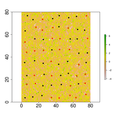
Refer to caption
Refer to caption
Figure 10: The plots show the structure of data in our simulation. On the right is a point intervention. Each treated point is marked in red and each untreated one is marked in black. Colors in the background indicate the outcome values. On the right is a polygon intervention. Treated and untreated nodes are marked by red and black borders, respectively. It also demonstrates buffers around each intervention polygon.
Refer to caption
Refer to caption
Refer to caption
Refer to caption
Figure 11: The top-left plot shows the bias of the Horvitz-Thompson estimator in the Bernoulli point intervention. The top-right plot shows the bias of the Hajek estimator in a point intervention where the treatment is assigned following complete randomization. The bottom-right plot shows the bias of the Hajek estimator in the Bernoulli point intervention, when the effect function equals zero across all the distance values. The red curves indicate the true AME curve and each grey curve represents the estimates under one random assignment. The bottom-right plot compares the simulated 95% confidence intervals with the averages of 95% Spatial HAC confidence intervals under the null effect function.
Refer to caption
Refer to caption
Refer to caption
Refer to caption
Figure 12: These plots show results from the kernel regression estimator in the Bernoulli point intervention. The top-left plot presents the bias of the estimator. The top-right plot compares the simulated 95% confidence intervals with the averages of 95% Spatial HAC confidence intervals. The two plots on the bottom demonstrate how the MSE and the coverage rate of the estimator varies with sample sizes.
Refer to caption
Refer to caption
Refer to caption
Refer to caption
Figure 13: These plots show results from the Hajek estimator in the polygon intervention. The top-left plot presents the bias of the estimator. The top-right plot compares the simulated 95% confidence intervals with the averages of 95% Spatial HAC confidence intervals. The two plots on the bottom demonstrate how the MSE and the coverage rate of the estimator varies with sample sizes.

B.3 Extra results from application
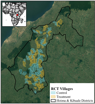
Refer to caption
Refer to caption
Figure 14: Top plot: The Global Forest Cover (GFC) dataset over a subset of the study area showing forest cover for 2012, 2013, and forest loss in 2012 (Hansen et al., 2013). Bottom plots: study area of randomized control trial for a PES program in Hoima and Kibaale district in Uganda, from Jayachandran et al. (2017). Boundaries of treatment (60) and control (61) villages were digitized using publicly available data and published maps.
Refer to caption
Refer to caption
Refer to caption
Refer to caption
Figure 15: The plots on the top show results from the Hajek estimator (left) or the kernel regression estimator (right), when each village in the experiment is treated as a point rather than a polygon. We calculate distances from the geographic center of each village and calculate the circle averages across all the pixels on the edges of the circles. The black solid line represents the estimated AME at each distance value. The black dotted lines around it are the 95% spatial HAC confidence intervals. The blue dotted lines are the 2.5% and 97.5% quantiles of the effect estimates under sharp null. The plots on the bottom show how the 95% spatial HAC confidence intervals based on the Hajek estimator (left) or the kernel regression estimator (right) vary with the selected cutoff value. We consider five different choices, all the way from 4 km to 20 km.

References

  • Arbia (2006) Arbia, G. (2006). Spatial econometrics: statistical foundations and applications to regional convergence. New York: Springer.
  • Aronow and Samii (2017) Aronow, P. M. and C. Samii (2017). Estimating average causal effects under general interference, with application to a social network experiment. Annals of Applied Statistics 11(4), 1912–1947.
  • Calonico et al. (2014) Calonico, S., M. D. Cattaneo, and R. Titiunik (2014). Robust nonparametric confidence intervals for regression-discontinuity designs. Econometrica 82(6), 2295–2326.
  • Conley (1999) Conley, T. G. (1999). GMM estimation with cross sectional dependence. Journal of Econometrics 92, 1–45.
  • Cox (1958) Cox, D. R. (1958). Planning of Experiments. Wiley.
  • Darmofal (2015) Darmofal, D. (2015). Spatial Analysis for the Social Sciences. Cambridge: Cambridge University Press.
  • Hainmueller et al. (2019) Hainmueller, J., J. Mummolo, and Y. Xu (2019). How much should we trust estimates from multiplicative interaction models? simple tools to improve empirical practice. Political Analysis 27(2), 163–192.
  • Halloran and Struchiner (1995) Halloran, M. E. and C. J. Struchiner (1995). Causal inference in infectious diseases. Epidemiology, 142–151.
  • Hansen et al. (2013) Hansen, M. C., P. V. Potapov, R. Moore, M. Hancher, S. A. Turubanova, A. Tyukavina, D. Thau, S. V. Stehman, S. J. Goetz, T. R. Loveland, et al. (2013). High-resolution global maps of 21st-century forest cover change. science 342(6160), 850–853.
  • Hu et al. (2022) Hu, Y., S. Li, and S. Wager (2022). Average direct and indirect causal effects under interference. Biometrika.
  • Hudgens and Halloran (2008) Hudgens, M. G. and M. E. Halloran (2008). Toward causal inference with interference. Journal of the American Statistical Association 103(482), 832–842.
  • Imbens and Rubin (2015) Imbens, G. W. and D. B. Rubin (2015). Causal Inference for Statistics, Social, and Biomedical Sciences: An Introduction. Cambridge: Cambridge University Press Press.
  • Jayachandran et al. (2017) Jayachandran, S., J. de Laat, E. F. Lambin, C. Y. Stanton, R. Audy, and N. E. Thomas (2017). Cash for carbon: A randomized trial of payments for ecosystem services to reduce deforestation. Science 357(6348), 267–273.
  • Jenish (2016) Jenish, N. (2016). Spatial semiparametric model with endogenous regressors. Econometric Theory 32(3), 714–739.
  • Jenish and Prucha (2009) Jenish, N. and I. R. Prucha (2009). Central limit theorems and uniform laws of large numbers for arrays of random fields. Journal of Econometrics 150(1), 86–98.
  • Kelejian and Piras (2017) Kelejian, H. and G. Piras (2017). Spatial Econometrics. New York: Elsevier.
  • Kojevnikov et al. (2021) Kojevnikov, D., V. Marmer, and K. Song (2021). Limit theorems for network dependent random variables. Journal of Econometrics 222(2), 882–908.
  • Leung (2022a) Leung, M. P. (2022a). Causal inference under approximate neighborhood interference. Econometrica 90(1), 267–293.
  • Leung (2022b) Leung, M. P. (2022b). Rate-optimal cluster-randomized designs for spatial interference. The Annals of Statistics 50(5), 3064–3087.
  • Li and Wager (2022) Li, S. and S. Wager (2022). Random graph asymptotics for treatment effect estimation under network interference. The Annals of Statistics 50(4), 2334–2358.
  • Miguel and Kremer (2004) Miguel, E. and M. Kremer (2004). Worms: identifying impacts on education and health in the presence of treatment externalities. Econometrica 72(1), 159–217.
  • Ogburn et al. (2020) Ogburn, E. L., O. Sofrygin, I. Diaz, and M. J. van der Laan (2020). Causal inference for social network data. arXiv preprint arXiv:1705.08527.
  • Opsomer et al. (2001) Opsomer, J., Y. Wang, and Y. Yang (2001). Nonparametric regression with correlated errors. Statistical Science, 134–153.
  • Papadogeorgou et al. (2020) Papadogeorgou, G., K. Imai, J. Lyall, and F. Li (2020). Causal inference with spatio-temporal data: estimating the effects of airstrikes on insurgent violence in iraq. arXiv preprint arXiv:2003.13555.
  • Raič (2004) Raič, M. (2004). A multivariate clt for decomposable random vectors with finite second moments. Journal of Theoretical Probability 17(3), 573–603.
  • Ross et al. (2011) Ross, N. et al. (2011). Fundamentals of Stein’s method. Probability Surveys 8, 210–293.
  • Rubin (2005) Rubin, D. B. (2005). Causal inference using potential outcomes: Design, modeling, decisions. Journal of the American Statistical Association 100, 322–331.
  • Samii and Aronow (2012) Samii, C. and P. M. Aronow (2012). On equivalencies between design-based and regression-based variance estimators for randomized experiments. Statistics and Probability Letters 82(2), 365–370.
  • Särndal et al. (1992) Särndal, C.-E., B. Swensson, and J. Wretman (1992). Model Assisted Survey Sampling. New York: Springer.
  • Sävje et al. (2021) Sävje, F., P. M. Aronow, and M. G. Hudgens (2021). Average treatment effects in the presence of unknown interference. The Annals of Statistics 49(2), 673–701.
  • VanderWeele and Tchetgen (2011) VanderWeele, T. J. and E. J. T. Tchetgen (2011). Effect partitioning under interference in two-stage randomized vaccine trials. Statistics & probability letters 81(7), 861–869.
  • Wang (2021) Wang, Y. (2021). Causal inference under temporal and spatial interference. arXiv preprint arXiv:2106.15074.
  • Young (2015) Young, A. (2015). Improved, nearly exact, statistical inference with robust and clustered covariance matrices using effective degrees of freedom corrections. Unpublished Manuscript, London School of Economics.
  • Zigler and Papadogeorgou (2018) Zigler, C. M. and G. Papadogeorgou (2018). Bipartite causal inference with interference. arXiv:1807.08660 [stat.ME].