Efficient Optimization Methods for Extreme Similarity Learning with Nonlinear Embeddings
Abstract.
We study the problem of learning similarity by using nonlinear embedding models (e.g., neural networks) from all possible pairs. This problem is well-known for its difficulty of training with the extreme number of pairs. For the special case of using linear embeddings, many studies have addressed this issue of handling all pairs by considering certain loss functions and developing efficient optimization algorithms. This paper aims to extend results for general nonlinear embeddings. First, we finish detailed derivations and provide clean formulations for efficiently calculating some building blocks of optimization algorithms such as function, gradient evaluation, and Hessian-vector product. The result enables the use of many optimization methods for extreme similarity learning with nonlinear embeddings. Second, we study some optimization methods in detail. Due to the use of nonlinear embeddings, implementation issues different from linear cases are addressed. In the end, some methods are shown to be highly efficient for extreme similarity learning with nonlinear embeddings.
1. Introduction
Many applications can be cast in the problem of learning similarity between a pair of two entities referred to as the left and the right entities respectively. For example, in recommender systems, the similarity of a user-item pair indicates the preference of the user on the item. In search engines, the similarity of a query-document pair can be used as the relevance between the query and the document. In multi-label classifications, for any instance-label pair with high similarity, the instance can be categorized to the label.
A popular approach for similarity learning is to train an embedding model as the representation of each entity in the pair, such that any pair with high similarity are mapped to two close vectors in the embedding space, and vice versa. For the choice of the embedding model, some recent works (Zhong et al., 2019) report the superiority of nonlinear over conventional linear ones. A typical example of applying nonlinear embedding models is the two-tower structure illustrated in Figure 1, where a multi-layer neural network serves as the embedding model of each entity. Some successful uses in real-world applications have been reported (Huang et al., 2013; Elkahky et al., 2015; Yang et al., 2018; Yi et al., 2019; Huang et al., 2020).
While many works only consider observed pairs for similarity learning, more and more works argue that better performance can be achieved by considering all possible pairs. For example, recommender systems with implicit feedback face a one-class scenario, where all observed pairs are labeled as similar while the dissimilar ones are missing. To achieve better similarity learning, a widely-used setting (Pan and Scholz, 2009; Yu et al., 2014, 2017b) is to include all unobserved pairs as dissimilar ones. Another example is counterfactual learning (Yuan et al., 2019a; Wang et al., 2019), where because the observed pairs carry the selection bias caused by confounders, an effective way to eliminate the bias is to additionally consider the unobserved pairs by imputing their labels.
However, for many real-world scenarios, both the number of left entities and the number of right entities can be tremendous. The learning procedure is challenging as a prohibitive cost occurs by directly applying any optimization algorithm. To avoid the complexity, one can subsample unobserved pairs, but it has been shown that such subsampled settings are inferior to the non-subsampled setting (Pan et al., 2008; Yu et al., 2017a). We refer to the problem of the similarity learning from extremely large pairs as extreme similarity learning.
An illustration of the two-tower structure; modified from (Rendle et al., 2020).
To tackle the high complexity, the aforementioned works that can handle all pairs consider a loss function with a certain structure for the unobserved pairs. Then they are able to replace the complexity with a much smaller one. In particular, the function value, gradient, or other information can be calculated in cost, so various types of optimization methods can be considered. Most exiting works consider linear embeddings (e.g., matrix factorization in (Pan and Scholz, 2009; He et al., 2016; Yu et al., 2017a)), where the optimization problem is often in a multi-block convex form. Thus many consider a block-wise setting to sequentially minimize convex sub-problems. The needed gradient or other information on each block of variables can also be calculated in .
If general nonlinear embeddings are considered, so far few works have studied the optimization algorithm. This work aims to fill the gap with the following main contributions.
-
•
To calculate function value, gradient, or other information in cost, the extension from cases in linear embeddings seems to be possible, but detailed derivations have not been available. We finish tedious calculations and provide clean formulations. This result enables the use of many optimization methods for extreme similarity learning with nonlinear embeddings.
-
•
We then study some optimization methods in detail. Due to the use of nonlinear embeddings, some implementation issues different from linear cases are addressed. In the end, some methods are shown to be highly efficient for extreme similarity learning with nonlinear embeddings.
The paper is organized as follows. A review on extreme similarity learning is in Section 2. We derive efficient computation for some important components in Section 3. In Section 4, we demonstrate that many optimization algorithms can be used for extreme similarity learning with nonlinear embeddings. Section 5 describes some implementation issues. Finally, we present experiments on large-scale data sets in Section 6, and conclude in Section 7. Table 1 gives main notations in this paper. The supplementary materials and data/code for experiments are available at https://www.csie.ntu.edu.tw/~cjlin/papers/similarity_learning/.
| Notation | Description |
|---|---|
| (left entity , right entity ) pair | |
| numbers of left entities and right entities | |
| feature vectors of a left entity and a right entity | |
| set of observed pairs | |
| a similarity function and its variables | |
| objective function | |
| observed incomplete similarity matrix | |
| similarity matrix predicted by | |
| imputed similarity matrix (for unobserved pairs) | |
| embedding models of left and right entities | |
| embedding vectors of left and right entities | |
| , | cost of operations related to , and |
2. Extreme Similarity Learning
We review extreme similarity learning problems.
2.1. Problem Formulation
Many real-world applications can be modeled as a learning problem with an incomplete similarity matrix of left entities and right entities. The set of observed pairs is denoted as where typically . Only are revealed. Besides , we assume that side features of left entities and of right entities are available. Our goal is to find a similarity function ,
| (1) |
where is the vectorized variables of with , and . For the similarity function, we consider the following dot product similarity that has been justified in a recent comparative study of similarity functions in recommender systems (Rendle et al., 2020)
where and are two embedding models that learn representations of left and right entities, respectively; see Figure 1. In this work, we focus on nonlinear embedding models. For convenience, we abbreviate and to and , respectively. We also write the embedding vectors as
| (2) |
so that
| (3) |
By considering all pairs, we learn through solving
| (4) |
where the objective function is
| (5) |
is an entry-wise twice-differentiable loss function convex in , is a twice-differentiable and strongly convex regularizer to avoid overfitting, and is the corresponding parameter. We assume is simple so that in all complexity analyses we ignore the costs related to , and . In (5), we further assume
| (6) |
where for any unobserved pair we impute as an artificial label of the similarity. For instance, in recommender systems with implicit feedback, by treating unobserved pairs as negative, usually or is considered.
Clearly (5) involves a summation of terms, so the cost of directly applying an optimization algorithm is prohibitively proportional to .
2.2. Linear Embedding Models
As mentioned in Section 1, most existing works of extreme similarity learning focus on linear embedding models. To avoid any cost occurs in solving the optimization problem, they consider a special kind of loss functions
| (7) |
where is any non-negative and twice-differentiable function convex in , and is a parameter for balancing the two kinds of losses. Two vectors , and are chosen so that is a cost associated with an unobserved pair. Besides, for the imputed label , it is required (Krichene et al., 2019; Yuan et al., 2019a) that
| (8) |
where are vectors output by the prior imputation model, and are fixed throughout training. For easy analysis, we assume that have the same length as . With the loss in (7), past works were able to reduce the cost to . The main reason is because derived computations on all and all can be obtained by using values solely related to and , respectively. A conceptual illustration is in the following equation.
| (9) |
The mainline of most past works is to incorporate more linear models into extreme similarity learning, which can range from simple matrix factorization (Pan and Scholz, 2009; He et al., 2016; Yu et al., 2017a) to complex models, e.g., matrix factorization with side information and (field-aware) factorization machines (Bayer et al., 2017; Yu et al., 2017b; Yuan et al., 2019b).
3. Information Needed in Optimization Algorithms
Most optimization methods involve a procedure that repeatedly calculates the function value, the gradient, and/or other information. For example, a gradient descent method must calculate the negative gradient as the direction for an update. Crucially, from past developments for linear embeddings, the cost mainly occurs in these building blocks of optimization algorithms. The aim of this section is to derive computation for these important components when nonlinear embeddings are applied.
3.1. From Linear to Nonlinear Embedding Models
We begin by discussing the differences between using linear and nonlinear embeddings. If linear embeddings are used, a key feature is that (4) becomes a multi-block convex problem. That is, (4) is reduced to a convex sub-problem when embedding variables of one side are fixed. Then existing works apply alternating least squares (Pan and Scholz, 2009), (block) coordinate descent (He et al., 2016; Yu et al., 2017a; Bayer et al., 2017; Yuan et al., 2019b), and alternating Newton method (Yu et al., 2017b; Yuan et al., 2019a) to sequentially solve each sub-problem by convex optimization techniques, which often iteratively calculate the following information.
-
•
Function value,
-
•
Gradient, and/or
-
•
Hessian-vector product
Thus a focus was on deriving operations for them.
If nonlinear embeddings are considered, in general (4) is not a block-convex problem. Thus a block-wise setting may not possess advantages so that optimization algorithms updating all variables together is a more natural choice. In any case, if we can obtain formulations for calculating the function value or the gradient over all variables, then the information over a block of variables is often in a simplified form. For example, the gradient over the block is a sub-vector of the whole gradient over . Therefore, in the rest of this section, we check the general scenario of considering all variables.
3.2. Evaluation of the Objective Value
The infeasible cost occurs if we directly compute in (5). To handle this, our idea is to follow past works of linear embeddings to consider (7) as the loss function.
By applying (7), (5) is equivalent to
| (10) |
where
| (11) |
The first term involves the summation of values, so with the bottleneck is on the second term .
Let and respectively represent the cost of operations related to the two nonlinear embedding models,111If neural networks are considered, operations such as forward or backward computation are considered. See more discussion in Section 5 and
| (12) |
where and are constant matrices, but and depend on . To compute in (10), we first compute and in time and store them in space. Then for each , from (3) and (8), we compute and in time. As a result, we can compute the entire in time.
For , we follow the idea in (9) to derive
| (13) |
where details are left in Appendix A.1. Later for gradient calculation we show details as a demonstration of using (9).
In (13), is a Frobenius inner product between two matrices,
| (14) | ||||
where are two diagonal matrices. As and have been pre-computed and cached in memory during computing , the matrices in (14) can be computed in time and cached in space. Then the Frobenius inner products between these matrices cost only time.
From complexities of and , the overall cost of evaluating is
| (15) |
3.3. Computation of Gradient Information
For defined in (5), the gradient is
| (16) |
Analogous to (5), it is impractical to directly compute with infeasible costs. For derivatives with respect to a vector, we let be a row vector, and later for operations such as , we let it be a matrix. In all other situations, a vector such as is a column vector.
From (7) and (10), in (16) is equivalent to
To calculate , let be a sparse matrix with
| (17) |
| (18) |
so with (17) we have
| (19) |
Let be tensors with
| (20) |
respectively. The top part of (19) can be computed by
| (21) |
where (21) is from (12) and the following definition of the tensor-matrix inner product
| (22) |
As the computation of the bottom part of (19) is similar, we omit the details. Then (19) can be written as
| (23) |
where and are first computed in time and stored in space. Then we compute and in time and space.
To calculate , from (3) and (11) we have
This and (18) imply that
| (24) | ||||
where the last two equalities follow from the idea in (9). From (14),
| (25) | ||||
so we can compute by
| (26) |
where (26) follows from (12), (20), and (22). As and have been pre-computed and cached in memory during computing , all matrices in (14) can be computed in time and cached in space. Then the right hand sides of in (26) can be computed in time as and are diagonal.
By combining (23) and (26), the entire can be efficiently computed by
| (27) |
which has a time complexity of
| (28) |
The terms come from calculating and in (23) and from , in (20). The procedure of evaluating is summarized in Algorithm 1.
From (15) and (28), the cost of one function evaluation is similar to that of one gradient evaluation.
3.4. Computation of Gauss-Newton Matrix-vector Products
For optimization methods using second-order information, commonly the product between Hessian and some vector is needed:
| (29) |
The Hessian of (5) is
| (30) |
Clearly, a direct calculation costs . However, before reducing the cost to , we must address an issue that is not positive definite. In past studies of linear embeddings (e.g., (Yu et al., 2017b; Chin et al., 2018; Yuan et al., 2019b)) the block-convex implies that for a strictly convex sub-problem, the Hessian is positive definite. Without such properties, here we need a positive definite approximation of . Following (Martens, 2010; Wang et al., 2015), we remove the second term in (30) to have the following Gauss-Newton matrix (Schraudolph, 2002)
| (31) |
which is positive definite from the convexity of in and the strong convexity of . The matrix-vector product becomes
| (32) |
From (11) we have
| (33) |
Following (10), we use (33) to re-write in (32) as
| (34) |
Let be some vector. By defining
| (35) |
from (18), we have
| (36) |
To compute in (34), we first compute
in time and store them in space. From (36), let be a sparse matrix with
which can be constructed in time. Then from (19) and similar to the situation of computing (21) and (23), we have
| (37) |
where and can be computed in time and space.
4. Optimization Methods for Extreme Similarity Learning with Nonlinear Embeddings
With the efficient computation of key components given in Section 3, we demonstrate that many optimization algorithms can be used. While block-wise minimization is applicable, we mentioned in Section 3.1 that without a block-convex , such a setting may not be advantageous. Thus in our discussion we focus more on standard optimization techniques that update all variables at a time.
4.1. (Stochastic) Gradient Descent Method
The standard gradient descent method considers the negative gradient direction
| (41) |
and update by
| (42) |
where is the step size. To ensure the convergence, usually a line-search procedure is conducted to find satisfying the following sufficient decrease condition
| (43) |
where is a pre-defined constant. During line search, given any , the corresponding function value must be calculated.
Combined with the cost of in (28) and the cost of in (15), the complexity of each gradient descent iteration is
| (44) |
where the term ‘1’ in comes from the cost of , and #LS is the number of line search steps.
In some machine learning applications, the gradient calculation is considered too expensive so an approximation using partial data samples is preferred. This leads to the stochastic gradient (SG) method. Without the full gradient, the update rule (42) may no longer lead to the decrease of the function value. Thus a line search procedure is not useful and the step size is often decided by some pre-defined rules or tuned as a hyper-parameter.
Unfortunately, it is known that for extreme similarity learning, a direct implementation of SG methods faces the difficulty of cost (e.g., (Yu et al., 2017a)). Now all pairs are considered as our data set and the cost of each SG step is proportional to the number of sampled pairs. Thus to go over all or most pairs many SG steps are needed and the cost is . In contrast, by techniques in Section 3.3 to calculate the gradient in cost, all pairs have been considered. A natural remedy is to incorporate techniques in Section 3.3 to the SG method. Instead of randomly selecting pairs in an SG step, (Krichene et al., 2019) proposed to select pairs in a set where and . If and , then by slightly modifying the derivation in (27), calculating the subsampled gradient involves instead of cost. Analogous to (28), the subsampled gradient on can be calculated in
where is the subset of observed pairs falling in . Then the complexity of each data pass of handling pairs via SG steps is
| (45) |
Thus the cost is deducted by a factor.
We consider another SG method that has been roughly discussed in (Krichene et al., 2019). The idea is to note that if and , then
| (46) | ||||
Then instead of selecting a subset from pairs, the setting becomes to select two independent sets for constructing the subsampled gradient, where and respectively corresponding to the first and the second summations in (46). Therefore, the task of going over pairs is replaced by selecting , and at a time to cover the whole after many SG steps. We leave details of deriving the subsampled gradient in Appendix A.2, and the complexity for the task comparable to going over all pairs by standard SG methods is
| (47) |
A comparison with (45) shows how (47) might alleviate the cost. This relies on and some appropriate choices of and . We refer to this method as the SG method based on (46).
The above setting is further extended in (Krichene et al., 2019) to Stochastic Online Gramian (SOGram), which applies a variance reduction scheme to improve the subsampled gradient. Details are in Appendix A.3.
We compare the above methods in Table 2 by checking the cost per data pass, which roughly indicates the process of handling pairs. Note that the total cost also depends on the number of data passes. In experiments we will see the trade-off between the cost per data pass and the number of total passes.
4.2. Methods Beyond Gradient Descent
We can further consider methods that incorporate the second-order information. By considering the following second-order Taylor expansion
| (48) |
Newton methods find a search direction by minimizing (48). However, this way of finding is often complicated and expensive. In the rest of this section, we discuss some practically viable options to use the second-order information.
4.2.1. Gauss-Newton Method
It is mentioned in Section 3.4 that Gauss-Newton matrix in (31) is a positive-definite approximation of . Thus replacing in (48) with leads to a convex quadratic optimization problem with the solution satisfying
| (49) |
However, for large-scale applications, not only is in (31) too large to be stored in memory, but the matrix inversion is also computationally expensive.
Following (Lin et al., 2008; Martens, 2010), we may solve (49) by the conjugate gradient (CG) method (Hestenes and Stiefel, 1952), which involves a sequence of matrix-vector products between and some vector . The derivation in Section 3.4 has shown how to calculate without explicitly forming and storing . Therefore, Gauss-Newton methods are a feasible approach for extreme similarity learning without the cost.
After a Newton direction is obtained, the line search procedure discussed in Section 4.1 is conducted to find a suitable to ensure the convergence. The complexity of each Newton iteration is
| (50) | ||||
where #CG is numbers of CG steps. The overall procedures of the CG method and the Gauss-Newton method are summarized in Appendix A.4.
4.2.2. Diagonal Scaling Methods
From (50), the CG procedure may be expensive so a strategy is to replace in (49) with a positive-definite diagonal matrix, which becomes a very loose approximation of . In this case, can be efficiently obtained by dividing each value in by the corresponding diagonal element. Methods following this idea are referred to as diagonal scaling methods.
For example, the AdaGrad algorithm (Duchi et al., 2011) is a popular diagonal scaling method. Given of current , AdaGrad maintains a zero-initialized diagonal matrix by
Then by considering , where is the identity matrix and is a small constant to ensure the invertibility, the direction is
| (51) |
In comparison with the gradient descent method, the extra cost is minor in , where is the total number of variables. Instead of using the full , this method can be extended to use subsampled gradient by the SG framework discussed in Section 4.1.
5. Implementation Details
So far we used and to represent the cost of operations on nonlinear embeddings. Here we discuss more details if automatic differentiation is employed for easily trying different network architectures. To begin, note that is the Jacobian of . Transposed Jacobian-vector products are used in for all methods and for the Gauss-Newton method. In fact, (27) and (40) are almost in the same form. It is known that for such an operation, the reverse-mode automatic differentiation (i.e., back-propagation) should be used so that only one pass of the network is needed (Baydin et al., 2018). For feedforward networks, including extensions such as convolutional networks, the cost of a backward process is within a constant factor of the forward process for computing the objective value (e.g., Section 5.2 of (Wang et al., 2020)). The remaining major operation to be discussed is the Jacobian-vector product in (35) in Section 4.2.1. This operation can be implemented with the forward-mode automatic differentiation in just one pass (Baydin et al., 2018), and the cost is also within a constant factor of the cost of forward objective evaluation.333See, for example, the discussion at https://www.csie.ntu.edu.tw/~cjlin/courses/optdl2021/slides/newton_gauss_newton.pdf. We conclude that if neural networks are used, using and as the cost of nonlinear embeddings is suitable.
Neural networks are routinely trained on GPU instead of CPU for better efficiency, but the smaller memory of GPU causes difficulties for larger problems or network architectures. This situation is even more serious for our case because some other matrices besides the two networks are involved; see (27) and (40). We develop some techniques to make large-scale training feasible, where details are left in supplementary materials.
6. Experiments
In this section, after presenting our experimental settings, we compare several methods discussed in Section 4 in terms of the convergence speed on objective value decreasing and achieving the final test performance.
6.1. Experimental Settings
6.1.1. Data sets
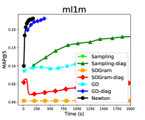
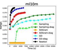
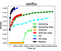
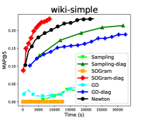
We consider three data sets of recommender systems with implicit feedback and one data set of link predictions. For data sets of recommender systems with implicit feedback, the target similarity of each observed user-item pair is 1, while those of the unobserved pairs are unrevealed. We consider ml1m, ml10m, and netflix provided by (Yu et al., 2017a). For the data set of link predictions, we follow (Krichene et al., 2019) to consider the problem of learning the intra-site links between Wikipedia pages, where the target similarity of each observed - pair is 1 if there is a link from to , and unrevealed otherwise. However, because the date information of the dump used in (Krichene et al., 2019) is not provided, their generated sets are irreproducible. We use the latest Wikipedia graph444https://dumps.wikimedia.org/simplewiki/20200901/ on pages in simple English and denote the generated data set as wiki-simple. For ml1m, ml10m and netflix, training and test sets are available. For wiki-simple, we follow (Krichene et al., 2019) to use a 9-to-1 ratio for the training/test split. The statistics of all data sets are listed in Table 3. Note that the aim here is to check the convergence behavior, so we do not need a validation set for hyper-parameter selection.
6.1.2. Model and Hyper-parameters
We train a two-tower neural network as in Figure 1. Both towers have three fully-connected layers, where the first two layers contain 256 hidden units equipped with ELU (Clevert et al., 2016) activation, and the last layer contains hidden units without activation. For all experiments, we choose the logistic loss , an L2 regularizer , and uniform weights in (7). For the imputed labels , we follow past works (Yu et al., 2017a, b) to apply a constant for any unobserved pair by setting , and . For and , for each data set, we consider a grid of hyper-parameter combinations and select the one achieving the best results on the test set. The selected and for each data set are listed in Table 3.
Comparison of different algorithms on four data sets.
| Data set | |||||
|---|---|---|---|---|---|
| ml1m | 6,037 | 3,513 | 517,770 | ||
| ml10m | 69,786 | 10,210 | 4,505,820 | ||
| netflix | 478,251 | 17,768 | 51,228,351 | ||
| wiki-simple | 85,270 | 55,695 | 5,478,549 |
6.1.3. Compared Optimization Methods
We compare seven optimization methods for extreme similarity learning, which are categorized into two groups. The first group includes the following three gradient-based methods discussed in Section 4.1.
-
•
GD: This is the gradient descent method. For each step, we compute by (27). To ensure the convergence, backtracking line search is conducted to find the step size .
- •
-
•
Sampling: This is the stochastic gradient method of choosing (Krichene et al., 2019). To make the number of steps in each data pass comparable to SOGram, for Sampling we set and , where is the ratio used in SOGram.
The step size in SOGram and Sampling is set to , , and respectively for ml1m, ml10m, netflix and wiki-simple. These values are from GD’s most used .
The second group includes the following four methods incorporating the second-order information discussed in Section 4.2.
- •
-
•
GD-diag, SOGram-diag, Sampling-diag: These three methods are respectively extended from GD, SOGram, and Sampling by applying the diagonal scaling in (51). For GD-diag, the same as GD, it finds by conducting backtracking line search. For SOGram-diag and Sampling-diag, we set .
For GD, Newton, and GD-diag, which conduct line search, we set for the sufficient decrease condition (43) and sequentially check in , where is the step size taken in the last iteration, and is doubled every five iterations to avoid being stuck with a small step size.
6.1.4. Environment and Implementation
We use TensorFlow (Abadi et al., 2016) compiled with Intel® Math Kernel Library (MKL) to implement all algorithms. Because most operations are matrix-based and MKL is optimized for such operations, our implementation should be sufficiently efficient. For sparse operations involving iterating (e.g., and ), we implement them by NumPy (Harris et al., 2020) and a C extension, where we parallelize these operations by OpenMP. As our applied neural networks described in Section 6.1.2 are not complex, we empirically do not observe many advantages of GPU over CPU on the running time. Thus all experiments are conducted on a Linux machine with 10 cores of Intel® Core™ i7-6950X CPUs and 128GB memory.
6.1.5. Evaluation Criterion of Test Performance
On test sets, we report mean average precision (MAP) on top- ranked entities. For left entity , let be the set of its similar right entities in the test set, and be the set of top- right entities with the highest predicted similarity. We define
| (52) |
where is the number of left entities in the test set.
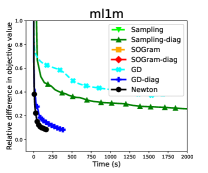
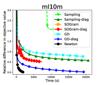
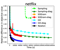
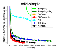
6.2. A Comparison on the Convergence Speed
We first investigate the relationship between the running time and the relative difference in objective value
where is the lowest objective value reached among all settings. The result is presented in Figure 2(a).
For the three gradient-based methods, SOGram, and Sampling are slower than GD. This situation is different from that of training general neural networks, where SG are the dominant methods. The reason is that though Sampling and SOGram take more iterations than GD in each data pass, from Table 2, they have much higher complexity per data pass.
For GD-diag, SOGram-diag, Sampling-diag, and Newton, which incorporate the second-order information, they are consistently faster than gradient-based methods. Specifically, between Newton and GD, the key difference is that Newton additionally considers the second-order information for yielding each direction. The great superiority of Newton confirms the importance of leveraging the second-order information. By comparing GD-diag and GD, we observe that GD-diag is much more efficient. Though both have similar complexities for obtaining search directions, GD-diag leverages partial second-order information from AdaGrad’s diagonal scaling. However, the effect of the diagonal scaling is limited, so GD-diag is slower than Newton. Finally, GD-diag is still faster than SOGram-diag, Sampling-diag as in the case of without diagonal scaling.
Next, we present in Figure 2(b) the relationship between the running time and MAP@5 evaluated on test sets. It is observed that a method with faster convergence in objective values is also faster in MAP@5.
7. Conclusions
In this work, we study extreme similarity learning with nonlinear embeddings. The goal is to alleviate the cost in the training process. While this topic has been well studied for the situation of using linear embeddings, a systematic study for nonlinear embeddings was lacking. We fill the gap in the following aspects. First, for important operations in optimization algorithms such as function and gradient evaluation, clean formulations with cost are derived. Second, these formulations enable the use of many optimization algorithms for extreme similarity learning with nonlinear embedding models. We detailedly discuss some of them and check implementation issues. Experiments show that efficient training by some algorithms can be achieved.
Acknowledgements.
We would like to thank Hong Zhu, Yaxu Liu, and Jui-Nan Yen for helpful discussions. This work was supported by MOST of Taiwan grant 107-2221-E-002-167-MY3.References
- (1)
- Abadi et al. (2016) Martin Abadi, Paul Barham, Jianmin Chen, Zhifeng Chen, Andy Davis, Jeffrey Dean, Matthieu Devin, Sanjay Ghemawat, Geoffrey Irving, Michael Isard, Manjunath Kudlur, Josh Levenberg, Rajat Monga, Sherry Moore, Derek G. Murray, Benoit Steiner, Paul Tucker, Vijay Vasudevan, Pete Warden, Martin Wicke, Yuan Yu, and Xiaoqiang Zheng. 2016. TensorFlow: A system for large-scale machine learning. In OSDI.
- Baydin et al. (2018) Atilim Gunes Baydin, Barak A. Pearlmutter, Alexey Andreyevich Radul, and Jeffrey Mark Siskind. 2018. Automatic differentiation in machine learning: a survey. JMLR 18 (2018), 1–43.
- Bayer et al. (2017) Immanuel Bayer, Xiangnan He, Bhargav Kanagal, and Steffen Rendle. 2017. A generic coordinate descent framework for learning from implicit feedback. In WWW.
- Chin et al. (2018) Wei-Sheng Chin, Bo-Wen Yuan, Meng-Yuan Yang, and Chih-Jen Lin. 2018. An Efficient Alternating Newton Method for Learning Factorization Machines. ACM TIST 9 (2018), 72:1–72:31.
- Clevert et al. (2016) Djork-Arné Clevert, Thomas Unterthiner, and Sepp Hochreiter. 2016. Fast and Accurate Deep Network Learning by Exponential Linear Units (ELUs). In ICLR.
- Duchi et al. (2011) John Duchi, Elad Hazan, and Yoram Singer. 2011. Adaptive Subgradient Methods for Online Learning and Stochastic Optimization. JMLR 12 (2011), 2121–2159.
- Elkahky et al. (2015) Ali Mamdouh Elkahky, Yang Song, and Xiaodong He. 2015. A multi-view deep learning approach for cross domain user modeling in recommendation systems. In WWW.
- Harris et al. (2020) Charles R. Harris, K. Jarrod Millman, Stéfan J. van der Walt, Ralf Gommers, Pauli Virtanen, David Cournapeau, Eric Wieser, Julian Taylor, Sebastian Berg, Nathaniel J Smith, et al. 2020. Array programming with NumPy. Nature 585, 7825 (2020), 357–362.
- He et al. (2016) Xiangnan He, Hanwang Zhang, Min-Yen Kan, and Tat-Seng Chua. 2016. Fast matrix factorization for online recommendation with implicit feedback. In SIGIR.
- Hestenes and Stiefel (1952) Magnus Rudolph Hestenes and Eduard Stiefel. 1952. Methods of Conjugate Gradients for Solving Linear Systems. JRNBS 49 (1952), 409–436.
- Huang et al. (2020) Jui-Ting Huang, Ashish Sharma, Shuying Sun, Li Xia, David Zhang, Philip Pronin, Janani Padmanabhan, Giuseppe Ottaviano, and Linjun Yang. 2020. Embedding-based Retrieval in Facebook Search. In KDD.
- Huang et al. (2013) Po-Sen Huang, Xiaodong He, Jianfeng Gao, Li Deng, Alex Acero, and Larry Heck. 2013. Learning deep structured semantic models for web search using clickthrough data. In CIKM.
- Krichene et al. (2019) Walid Krichene, Nicolas Mayoraz, Steffen Rendle, Li Zhang, Xinyang Yi, Lichan Hong, Ed Chi, and John Anderson. 2019. Efficient Training on Very Large Corpora via Gramian Estimation. In ICLR.
- Lin et al. (2008) C.-J. Lin, R. C. Weng, and S. S. Keerthi. 2008. Trust region Newton method for large-scale logistic regression. JMLR 9 (2008), 627–650.
- Martens (2010) James Martens. 2010. Deep learning via Hessian-free optimization. In ICML.
- Pan and Scholz (2009) Rong Pan and Martin Scholz. 2009. Mind the Gaps: Weighting the Unknown in Large-scale One-class Collaborative Filtering. In KDD.
- Pan et al. (2008) Rong Pan, Yunhong Zhou, Bin Cao, Nathan N Liu, Rajan Lukose, Martin Scholz, and Qiang Yang. 2008. One-class collaborative filtering. In ICDM.
- Rendle et al. (2020) Steffen Rendle, Walid Krichene, Li Zhang, and John Anderson. 2020. Neural Collaborative Filtering vs. Matrix Factorization Revisited. In RecSys.
- Schraudolph (2002) Nicol N. Schraudolph. 2002. Fast curvature matrix-vector products for second-order gradient descent. Neural Comput. 14 (2002), 1723–1738.
- Wang et al. (2015) Chien-Chih Wang, Chun-Heng Huang, and Chih-Jen Lin. 2015. Subsampled Hessian Newton Methods for Supervised Learning. Neural Comput. 27 (2015), 1766–1795.
- Wang et al. (2020) Chien-Chih Wang, Kent Loong Tan, and Chih-Jen Lin. 2020. Newton Methods for Convolutional Neural Networks. ACM TIST 11 (2020), 19:1–19:30.
- Wang et al. (2019) Xiaojie Wang, Rui Zhang, Yu Sun, and Jianzhong Qi. 2019. Doubly robust joint learning for recommendation on data missing not at random. In ICML.
- Yang et al. (2018) Yinfei Yang, Steve Yuan, Daniel Cer, Sheng-Yi Kong, Noah Constant, Petr Pilar, Heming Ge, Yun-Hsuan Sung, Brian Strope, and Ray Kurzweil. 2018. Learning Semantic Textual Similarity from Conversations. In RepL4NLP.
- Yi et al. (2019) Xinyang Yi, Ji Yang, Lichan Hong, Derek Zhiyuan Cheng, Lukasz Heldt, Aditee Kumthekar, Zhe Zhao, Li Wei, and Ed Chi. 2019. Sampling-Bias-Corrected Neural Modeling for Large Corpus Item Recommendations. In RecSys.
- Yu et al. (2017a) Hsiang-Fu Yu, Mikhail Bilenko, and Chih-Jen Lin. 2017a. Selection of Negative Samples for One-class Matrix Factorization. In SDM.
- Yu et al. (2017b) Hsiang-Fu Yu, Hsin-Yuan Huang, Inderjit S. Dihillon, and Chih-Jen Lin. 2017b. A Unified Algorithm for One-class Structured Matrix Factorization with Side Information. In AAAI.
- Yu et al. (2014) Hsiang-Fu Yu, Prateek Jain, Purushottam Kar, and Inderjit S. Dhillon. 2014. Large-scale Multi-label Learning with Missing Labels. In ICML.
- Yuan et al. (2019a) Bowen Yuan, Jui-Yang Hsia, Meng-Yuan Yang, Hong Zhu, Chihyao Chang, Zhenhua Dong, and Chih-Jen Lin. 2019a. Improving Ad Click Prediction by Considering Non-displayed Events. In CIKM.
- Yuan et al. (2019b) Bowen Yuan, Meng-Yuan Yang, Jui-Yang Hsia, Hong Zhu, Zhirong Liu, Zhenhua Dong, and Chih-Jen Lin. 2019b. One-class Field-aware Factorization Machines for Recommender Systems with Implicit Feedbacks. Technical Report. National Taiwan Univ.
- Zhong et al. (2019) Kai Zhong, Zhao Song, Prateek Jain, and Inderjit S Dhillon. 2019. Provable Non-linear Inductive Matrix Completion. In NIPS.
Appendix A Appendix
A.1. Detailed Derivation of
To compute , we rewrite it as
| (53) |
To calculate (53), we need matrices listed in (14). For and , they are constant matrices throughout the training process, so we can calculate them and within at the beginning. Thus this cost can be omitted in the complexity analysis. For other matrices in (14), and are needed, but they have been pre-computed and cached in memory during computing . Thus all matrices in (14) can be obtained in time and cached in space. Then in (53), the Frobenius inner products between these matrices cost only time. Through combining calculation discussed in Section 3.2, Algorithm 2 summarizes the procedure of evaluating the objective function.
A.2. Detailed Derivation of a Stochastic Gradient Method Based on (46)
From (46), by defining and , in (10) can be written as
| (54) |
Then in (24) can be rewritten as
| (55) | ||||
| (56) |
where similar to (14), we define
| (57) | ||||
and we omit details from (55) to (56) as the derivations are similar to those between (24) and (26).
On the other hand, from (17) and (18), we write as
| (58) |
Because both (56) and (58) are now operations summing over , can be written as
| (59) |
To derive a subsampled approach, we must consider two subsets and because from (57), two summations respectively over are involved in the above gradient. This results in the following estimate of .
| (60) |
where
| (61) | ||||
To make (60) an unbiased estimate of , we need that and are independent of each other, and have the scaling factors , respectively in (60) and (61).
Because and are independent subsets, we can swap them in (60) to have another estimate of . Then four matrices and similar to those in (61) must be calculated, but the summations are now over . In the end, the two subsampled gradients can be averaged.
Similar to the discussion on (14) and (27), for each pair of and , (59) can be computed in
| (62) |
time. We take term as an example to illustrate the difference from (27). Now for matrices in (61), each involves cost, but for those in (14), or are needed. Therefore, from (28) to (62), we can see the term should be replaced by .
Next we check the complexity. We have mentioned in Section 4.1 that the task of going over all pairs is now replaced by sampling to cover . Thus the time complexity is by multiplying the steps and the cost in (62) for each SG step to have
| (63) |
A.3. Detailed Derivation of the SOGram Method
We discuss the Stochastic Online Gramian (SOGram) method proposed in (Krichene et al., 2019), which is very related to the method discussed in Section A.2. It considers a special case of the objective function in (54) by excluding and . From this we show that SOGram is an extension.
In (Krichene et al., 2019), they view matrices in (61) as estimates of matrices in (14). The main idea behind SOGram is to apply a variance reduction scheme to improve these estimates. Specifically, they maintain four zero-initialized matrices with the following exponentially averaged updates before each step
| (64) | ||||
where is a hyper-parameter for controlling the bias-variance tradeoff. Then they replace (60) with
| (65) |
which is considered as the subsampled gradient vector for each SG step.