How to Measure the Reproducibility of
System-oriented IR Experiments

Abstract.

Replicability and reproducibility of experimental results are primary concerns in all the areas of science and IR is not an exception. Besides the problem of moving the field towards more reproducible experimental practices and protocols, we also face a severe methodological issue: we do not have any means to assess when reproduced is reproduced. Moreover, we lack any reproducibility-oriented dataset, which would allow us to develop such methods.

To address these issues, we compare several measures to objectively quantify to what extent we have replicated or reproduced a system-oriented IR experiment. These measures operate at different levels of granularity, from the fine-grained comparison of ranked lists, to the more general comparison of the obtained effects and significant differences. Moreover, we also develop a reproducibility-oriented dataset, which allows us to validate our measures and which can also be used to develop future measures.

1. Introduction

We are today facing the so-called reproducibility crisis (Baker, 2016; Open Science Collaboration, 2015) across all areas of science, where researchers fail to reproduce and confirm previous experimental findings. This crisis obviously involves also the more recent computational and data-intensive sciences (Freire et al., 2016; National Academies of Sciences, Engineering, and Medicine, 2019), including hot areas such as artificial intelligence and machine learning (Gibney, 2020). For example, Baker (2016) reports that roughly 70% of researchers in physics and engineering fail to reproduce someone else’s experiments and roughly 50% fail to reproduce even their own experiments.

Information Retrieval (IR) is not an exception and researchers are paying more and more attention to what the reproducibility crisis may mean for the field, even more with the raise of the new deep learning and neural approaches (Crane, 2018; Dacrema et al., 2019).

In addition to all the well-known barriers to reproducibility (Freire et al., 2016), a fundamental methodological question remains open: When we say that an experiment is reproduced, what exactly do we mean by it? The current attitude is some sort of “close enough”: researchers put any reasonable effort to understand how an approach was implemented and how an experiment was conducted and, after some (several) iterations, when they obtain performance scores which somehow resemble the original ones, they decide that an experimental result is reproduced. Unfortunately, IR completely lacks any means to objectively measure when reproduced is reproduced and this severely hampers the possibility both to assess to what extent an experimental result has been reproduced and to sensibly compare among different alternatives for reproducing an experiment.

This severe methodological impediment is not limited to IR but it has been recently brought up as a research challenge also in the 2019 report on “Reproducibility and Replicability in Science” by the US National Academies of Sciences, Engineering, and Medicine (2019, p. 62): “The National Science Foundation should consider investing in research that explores the limits of computational reproducibility in instances in which bitwise reproducibility is not reasonable in order to ensure that the meaning of consistent computational results remains in step with the development of new computational hardware, tools, and methods”. Another severe issue is that we lack any experimental collection specifically focused on reproducibility and this prevents us from developing and comparing measures to assess the extent of achieved reproducibility.

In this paper, we tackle both these issues. Firstly, we consider different measures which allow for comparing experimental results at different levels from most specific to most general: the ranked lists of retrieved documents; the actual scores of effectiveness measures; the observed effects and significant differences. As you can note these measures progressively depart more and more from the “bitwise reproducibility” (National Academies of Sciences, Engineering, and Medicine, 2019) which in the IR case would mean producing exactly identical ranked lists of retrieved documents. Secondly, starting from TREC data, we develop a reproducibility-oriented dataset and we use it to compare the presented measures.

The paper is organized as follows: Section 2 discusses related work; Section 3 introduces the evaluation measures under investigation; Section 4 describes how we created the reproducibility-oriented dataset; Section 5 presents the experimental comparison of the evaluation measures; finally, Section 6 draws some conclusions and outlooks future work.

2. Related Work

In defining what repeatability, replicability, reproducibility, and other of the so-called r-words are (Plesser, 2018), De Roure (2014) lists 21 r-words grouped in 6 categories, which range from scientific method to understanding and curation. In this paper, we broadly align with the definition of replicability and reproducibility currently adopted by the Association for Computing Machinery (ACM):

• Replicability (different team, same experimental setup): the measurement can be obtained with stated precision by a different team using the same measurement procedure, the same measuring system, under the same operating conditions, in the same or a different location on multiple trials. For computational experiments, an independent group can obtain the same result using the author’s own artifacts;

• Reproducibility (different team, different experimental setup): the measurement can be obtained with stated precision by a different team, a different measuring system, in a different location on multiple trials. For computational experiments, an independent group can obtain the same result using artifacts which they develop completely independently.

Reproducibility Efforts in IR

There have been and there are several initiatives related to reproducibility in IR. Since 2015, the ECIR conference hosts a track dedicated to papers which reproduce existing studies, and all the major IR conferences ask an assessment of the ease of reproducibility of a paper in their review forms. The SIGIR group has started a task force (Ferro and Kelly, 2018) to define what reproducibility is in system-oriented and user-oriented IR and how to implement the ACM badging policy in this context. Fuhr (2017, 2019) urged the community to not forget about reproducibility and discussed reproducibility and validity in the context of the CLEF evaluation campaign. The recent ACM JDIQ special issue on reproducibility in IR (Ferro et al., 2018a, b) provides an updated account of the state-of-the-art in reproducibility research as far as evaluation campaigns, collections, tools, infrastructures and analyses are concerned. The SIGIR 2015 RIGOR workshop (Arguello et al., 2015) investigated reproducibility, inexplicability, and generalizability of results and held a reproducibility challenge for open source software (Lin et al., 2016). The SIGIR 2019 OSIRRC workshop (Clancy et al., 2019) conducted a replicability challenge based on Docker containers.

CENTRE is an effort across CLEF (Ferro et al., 2018c; Ferro et al., 2019), TREC (Soboroff et al., 2019), and NTCIR (Sakai et al., 2019) to run a joint evaluation activity on reproducibility. One of the goals of CENTRE was to define measures to quantify to which extent experimental results were reproduced. However, the low participation in CENTRE prevented the development of an actual reproducibility-oriented dataset and hampered the possibility of developing and validating measures for reproducibility.

Measuring Reproducibility

To measure reproducibility, CENTRE exploited: Kendall’s $\tau$ (Kendall, 1948), to measure how close are the original and replicated list of documents; Root Mean Square Error (RMSE) (Kenney and Keeping, 1954), to quantify how close are the effectiveness scores of the original and replicated runs; and the Effect Ratio (ER) (Sakai et al., 2019), to quantify how close are the effects of the original and replicated/reproduced systems.

We compare against and improve with respect to previous work within CENTRE. Indeed, Kendall’s $\tau$ cannot deal with rankings that do not contain the same elements; CENTRE overcomes this issue by considering the union of the original and replicated rankings and comparing with respect to it; we show how this is a somehow pessimistic approach, penalizing the systems and propose to use Rank-Biased Overlap (RBO) (Webber et al., 2010), since it is natively capable to deal with rankings containing different elements. Furthermore, we complement Effect Ratio (ER) with the new Delta Relative Improvement (DeltaRI) score, to better grasp replicability and reproducibility in terms of absolute scores and to provide a visual interpretation of the effects. Finally, we propose to test replicability and reproducibility with paired and unpaired t-test (Student, 1908) respectively, and to use $p$-values as an estimate of replicability and reproducibility success.

To the best of our knowledge, inspired by the somehow unsuccessful experience of CENTRE, we are the first to systematically investigate measures for guiding replicability and reproducibility in IR, backing this with the development of a reproducibility-oriented dataset. As previously observed, there is a compelling need for reproducibility measures for computational and data-intensive sciences (National Academies of Sciences, Engineering, and Medicine, 2019), being the largest body of knowledge focused on traditional lab experiments and metrology (National Academies of Sciences, Engineering, and Medicine, 2016; ISO 5725-2:2019, 2019), and we try here to start addressing that need in the case of IR.

3. Proposed Measures

We first introduce our notation. In all cases we assume that the original run $r$ is available. For replicability (§ 3.1), both the original run $r$ and the replicated run $r^{\prime}$ contain documents from the original collection $C$. For reproducibility (§ 3.2), $r$ denotes the original run on the original collection $C$, while $r^{\prime}$ denotes the reproduced run on the new collection $D$. Topics are denoted by $j\in\{1,\ldots,n_{C}\}$ in $C$ and $j\in\{1,\ldots,n_{D}\}$ in $D$, while rank positions are denoted by $i$. $M$ is any IR evaluation measure e.g., P@10, AP, nDCG, where the superscript $C$ or $D$ refers to the collection. $M^{C}(r)$ is the vector of length $n_{C}$ where each component, $M_{j}^{C}(r)$, is the score of the run $r$ with respect to the measure $M$ and topic $j$. $\overline{M^{C}(r)}$ is the average score computed across topics.

3.1. Replicability

We evaluate replicability at different levels: (i) we consider the actual ordering of documents by using Kendall’s $\tau$ and Rank-Biased Overlap (RBO) (Webber et al., 2010); (ii) we compare the runs in terms of effectivenes with RMSE; (iii) we consider whether the overall effect can be replicated with Effect Ratio (ER) and Delta Relative Improvement (DeltaRI); and (iv) we compute statistical comparisons and consider the $p$-value of a paired t-test. While Kendall’s $\tau$, RMSE and ER were originally proposed for CENTRE, the other approaches has never been used for replicability.

It is worth mentioning that these approaches are presented from the most specific to the most general. Kendall’s $\tau$ and RBO compares the runs at document level, RMSE accounts for the performance at topic level, ER and DeltaRI focus on the overall performance by considering the average across topics, while the $t$-test can just inform us on the significant differences between the original and replicated runs. Moreover, perfect equality for Kendall’s $\tau$ and RBO implies perfect equality for RMSE, ER/DeltaRI and $t$-test, and perfect equality for RMSE implies perfect equality for ER/DeltaRI and $t$-test, while viceversa is in general not true.

As reference point, we consider the average score across topics of the original and replicated runs, called Average Retrieval Performance (ARP). Its delta represents the current “naive” approach to replicability, simply contrasting the average scores of the original and replicated runs.

Ordering of Documents

Kendall’s $\tau$ is computed as follows (Kendall, 1948):

(1) $$\tau_{j}(r,r^{\prime}) =\frac{P-Q}{\sqrt{\big{(}P+Q+U\big{)}\big{(}P+Q+V\big{)}}}$$

$$\bar{\tau}(r,r^{\prime}) =\frac{1}{n_{C}}\sum_{j=1}^{n_{C}}\tau_{j}(r,r^{\prime})$$

where $\tau_{j}(r,r^{\prime})$ is Kendall’s $\tau$ for the $j$-th topic, $P$ is the total number of concordant pairs (document pairs that are ranked in the same order in both vectors), $Q$ the total number of discordant pairs (document pairs that are ranked in opposite order in the two vectors), $U$ and $V$ are the number of ties, in $r$ and $r^{\prime}$ respectively.

This definition of Kendall’s $\tau$ is originally proposed for permutations of the same set of items, therefore it is not directly applicable whenever two rankings do not contain the same set of documents. However, this is not the case of real runs, which often return different sets of documents. Therefore, as done in CENTRE@CLEF (Ferro et al., 2018c; Ferro et al., 2019), we consider the correlation with respect to the union of the rankings. We refer to this method as Kendall’s $\tau$ Union. The underlying idea is to compare the relative orders of documents in the original and replicated rankings. For each topic, we consider the union of $r$ and $r^{\prime}$, by removing duplicate entries. Then we consider the rank positions of documents from the union in $r$ and $r^{\prime}$, obtaining two lists of rank positions. Finally, we compute the correlation between these two lists of rank positions. Note that, whenever two rankings contain the same set of documents, Kendall’s $\tau$ in Eq. (1) and Kendall’s $\tau$ Union are equivalent. To better understand how Kendall’s $\tau$ Union is defined, consider two rankings: $r=[d_{1},d_{2},d_{3}]$ and $r^{\prime}=[d_{1},d_{2},d_{4}]$, the union of $r$ and $r^{\prime}$ is $[d_{1},d_{2},d_{3},d_{4}]$, then the two lists of rank positions are $[1,2,3]$ and $[1,2,4]$ and the final Kendall’s $\tau$ is equal to $1$. Similarly consider $r=[d_{1},d_{2},d_{3},d_{4}]$ and $r^{\prime}=[d_{2},d_{5},d_{3},d_{6}]$, the union of $r$ and $r^{\prime}$ is $[d_{1},d_{2},d_{3},d_{4},d_{5},$ $d_{6}]$, then the two lists of rank positions are $[1,2,3,4]$ and $[2,5,3,6]$ and the final Kendall’s $\tau$ is equal to $2/3$.

We also consider Kendall’s $\tau$ on the intersection of the rankings instead of the union. As reported in (Sanderson and Soboroff, 2007), Kendall’s $\tau$ can be very noisy with small rankings and should be considered together with the size of the overlap between the $2$ rankings. However, this approach does not inform us on the rank positions of the common documents. Therefore, to seamlessly deal with rankings possibly containing different documents and to accout for their rank positions, we propose to use Rank-Biased Overlap (RBO) (Webber et al., 2010), which assumes $r$ and $r^{\prime}$ to be infinite runs:

(2) $$\text{RBO}_{j}(r,r^{\prime}) =(1-\phi)\sum_{i=1}^{\infty}\phi^{i-1}\cdot A_{i}$$

$$\overline{\text{RBO}}(r,r^{\prime}) =\frac{1}{n_{C}}\sum_{j=1}^{n_{C}}\text{RBO}_{j}(r,r^{\prime})$$

where $\text{RBO}_{j}(r,r^{\prime})$ is RBO for the $j$-th topic; $\phi\in[0,1]$ is a parameter to adjust the measure top-heaviness: the smaller $\phi$, the more top-weighted the measure; and $A_{i}$ is the proportion of overlap up to rank $i$, which is defined as the cardinality of the intersection between $r$ and $r^{\prime}$ up to $i$ divided by $i$. Therefore, RBO accounts for the overlap of two rankings and discounts the overlap while moving towards the end of the ranking, since it is more likely for two rankings to have a greater overlap when many rank positions are considered.

Effectiveness

As reported in CENTRE@CLEF (Ferro et al., 2018c; Ferro et al., 2019), we exploit Root Mean Square Error (RMSE) (Kenney and Keeping, 1954) to measure how close the effectiveness scores of the replicated and original runs are:

(3) $$\mathrm{RMSE}\left(M^{C}(r),M^{C}(r^{\prime})\right)=\sqrt{\frac{1}{n_{C}}\sum_{j=1}^{n_{C}}\big{(}M_{j}^{C}(r)-M_{j}^{C}(r^{\prime})\big{)}^{2}}$$

RMSE depends just on the evaluation measure and on the relevance label of each document, not on the actual documents retrieved by each run. Therefore, if two runs $r$ and $r^{\prime}$ retrieve different documents, but with the same relevance labels, then RMSE is not affected and returns a perfect replicability score equal to $0$; on the other hand, Kendall’s $\tau$ and RBO will be able to detect such differences.

Although RMSE and the naive comparison of ARP scores can be thought as similar approaches, by taking the squares of the absolute differences, RMSE penalizes large errors more. This can lead to different results, as shown in Section 5.

Overall Effect

In this case, we define a replication task from a different perspective, as proposed in CENTRE@NTCIR (Sakai et al., 2019). Given a pair of runs, $a$ and $b$, such that the advanced $a$-run has been reported to outperform the baseline $b$-run on the collection $C$, can another research group replicate the improvement of the advanced run over the baseline run on $C$? With this perspective, the per-topic improvements in the original and replicated experiments are:

(4) $$\Delta M_{j}^{C}=M_{j}^{C}(a)-M_{j}^{C}(b)\ ,\,\,\,\,\,\Delta^{\prime}M_{j}^{C}=M_{j}^{C}(a^{\prime})-M_{j}^{C}(b^{\prime})$$

where $a^{\prime}$ and $b^{\prime}$ are the replicated advanced and baseline runs respectively. Note that even if the $a$-run outperforms the $b$-run on average, the opposite may be true for some topics: that is, per-topic improvements may be negative.

Since IR experiments are usually based on comparing mean effectiveness scores, Effect Ratio (ER) (Sakai et al., 2019) focuses on the replicability of the overall effect as follows:

(5) $$\text{ER}\left(\Delta^{\prime}M^{C},\Delta M^{C}\right)=\frac{\overline{\Delta^{\prime}M^{C}}}{\overline{\Delta M^{C}}}=\frac{\frac{1}{n_{C}}\sum_{j=1}^{n_{C}}\Delta^{\prime}M_{j}^{C}}{\frac{1}{n_{C}}\sum_{j=1}^{n_{C}}\Delta M_{j}^{C}}$$

where the denominator of ER is the mean improvement in the original experiment, while the numerator is the mean improvement in the replicated experiment. Assuming that the standard deviation for the difference in terms of measure $M$ is common across experiments, ER is equivalent to the ratio of effect sizes (or standardised mean differences for the paired data case) (Sakai, 2018): hence the name.

$\text{ER}\leq 0$ means that the replicated $a$-run failed to outperform the replicated $b$-run: the replication is a complete failure. If $0<\text{ER}<1$, the replication is somewhat successful, but the effect is smaller compared to the original experiment. If $\text{ER}=1$, the replication is perfect in the sense that the original effect has been recovered as is. If $\text{ER}>1$, the replication is successful, and the effect is actually larger compared to the original experiment.

Note that having the same mean delta scores, i.e. $ER=1$, does not imply that the per-topic replication is perfect. For example, consider two topics $i$ and $j$ and assume that the original delta scores are $\Delta M_{i}^{C}=0.2$ and $\Delta M_{j}^{C}=0.8$ while the replicated delta scores are $\Delta^{\prime}M_{i}^{C}=0.8$ and $\Delta^{\prime}M_{j}^{C}=0.2$. Then ER for this experiment is equal to $1$. While this difference is captured by RMSE or Kendall’s $\tau$, which focus on a per-topic level, ER considers instead whether the sample effect size (standardised mean difference) can be replicated or not.

ER focuses on the effect of the $a$-run over the $b$-run, isolating it from other factors, but we may also want to account for absolute scores that are similar to the original experiment. Therefore, we propose to complement ER with Delta Relative Improvement (DeltaRI) and to plot ER against DeltaRI to visually interpret the replicability of the effects. We define DeltaRI as follows:

(6) $$\text{RI}=\frac{\overline{M^{C}(a)}-\overline{M^{C}(b)}}{\overline{M^{C}(b)}},\qquad\text{RI}^{\prime}=\frac{\overline{M^{C}(a^{\prime})}-\overline{M^{C}(b^{\prime})}}{\overline{M^{C}(b^{\prime})}}$$

where RI and $\text{RI}^{\prime}$ are the relative improvements for the original and replicated runs and $\overline{M^{C}(\cdot)}$ is the average score across topics. Now let DeltaRI be $\Delta\text{RI}(\text{RI},\text{RI}^{\prime})=\text{RI}-\text{RI}^{\prime}$. DeltaRI ranges in $[-1,1]$, $\Delta\text{RI}=0$ means that the relative improvements are the same for the original and replicated runs; when $\Delta\text{RI}>0$, the replicated relative improvement is smaller than the original relative improvement, and in case $\Delta\text{RI}<0$, it is larger. DeltaRI can be used in combination with ER, by plotting ER ($x$-axis) against DeltaRI ($y$-axis), as done in Figure 2. If $ER=1$ and $\Delta\text{RI}=0$ both the effect and the relative improvements are replicated, therefore the closer a point to $(1,0)$ the more successful the replication experiment. We can now divide the ER-DeltaRI plane in $4$ regions, corresponding to the $4$ quadrants of the cartesian plane:

• Region both $1$: ER $>0$ and DeltaRI $>0$, the replication is somehow successful in terms of effect sizes, but not in terms of absolute scores;

• Region $2$: ER $<0$ and DeltaRI $>0$, the replication is a failure both in terms of effect sizes and absolute scores;

• Region $3$: both ER $<0$ and DeltaRI $<0$, the replication is a failure in terms of effect sizes, but not in terms of absolute scores;

• Region $4$: ER $>0$ and DeltaRI $<0$, this means that the replication is somehow successful both in terms of effect sizes and absolute scores.

Therefore, the preferred region is Region $4$, with the condition that the best replicability runs are close to $(1,0)$.

Statistical Comparison

We propose to compare the original and replicated runs in terms of their statistical difference: we run a two-tailed paired $t$-test between the scores of $r$ and $r^{\prime}$ for each topic in $C$ with respect to an evaluation measure $M$. The $p$-value returned by the $t$-test informs on the extent to which $r$ is successfully replicated: the smaller the $p$ value, the stronger the evidence that $r$ and $r^{\prime}$ are significantly different, thus $r^{\prime}$ failed in replicating $r$.

Note that the $p$-value does not inform on the overall effect, i.e. we may know that $r^{\prime}$ failed to replicate $r$, but we cannot infer whether $r^{\prime}$ performed better or worse than $r$.

3.2. Reproducibility

Differently from replicability, for reproducibility the original and reproduced runs are not obtained on the same collection (different documents and/or topic sets), thus the original run cannot be used for direct comparison with the reproduced run. As a consequence, Kendall’s $\tau$, RBO, and RMSE in Section 3.1 cannot be applied to the reproducibility task. Therefore, hereinafter we focus on: (i) reproducing the overall effect with ER; (ii) comparing the original and reproduced runs with statistical tests.

Overall Effect

CENTRE@NTCIR (Sakai et al., 2019) defines ER for reproducibility as follows: given a pair of runs, $a$-run and $b$-run, where the $a$-run has been reported to outperform the $b$-run on a test collection $C$, can another research group reproduce the improvement on a different test collection $D$? The original per-topic improvements are the same as in Eq. (4), while the reproduced per-topic improvements are defined as in Eq. (4) by replacing $C$ with $D$. Therefore, the resulting Effect Ratio (ER) (Sakai et al., 2019) is defined as follows:

(7) $$\text{ER}(\Delta^{\prime}M^{D},\Delta M^{C})=\frac{\overline{\Delta^{\prime}M^{D}}}{\overline{\Delta M^{C}}}=\frac{\frac{1}{n_{D}}\sum_{j=1}^{n_{D}}\Delta^{\prime}M_{j}^{D}}{\frac{1}{n_{C}}\sum_{j=1}^{n_{C}}\Delta M_{j}^{C}}$$

where $n_{D}$ is the number of topics in $D$. Assuming that the standard deviation of a measure $M$ is common across experiments, the above version of ER is equivalent to the ratio of effect sizes (or standardised mean differences for the two-sample data case) (Sakai, 2018); it can then be interpreted in a way similar to the ER for replicability. Note that since we are considering the ratio of the mean improvements instead of the mean of the improvements ratio, Eq. (7) can be applied also when the number of topics in $C$ and $D$ is different.

Similarly to the replicability case, ER can be complemented with DeltaRI, whose definition is the same of Eq. (6), but $\text{RI}^{\prime}$ is computed over the new collection $D$, instead of the original collection $C$. DeltaRI has the same interpretation as in the replicability case, i.e. to show if the improvement in terms of relative scores in the reproduced experiment are similar to the original experiment.

Statistical Comparison

With a t-test, we can also handle the case when the original and the reproduced experiments are based on different datasets. In this case, we need to perform a two-tailed unpaired t-test to account, for the different subjects used in the comparison.

The unpaired t-test assumes equal variance and this is likely to not happen when, e.g., you have two different sets of topics in the two datasets. However, the unpaired t-test is known to be robust to such violations and Sakai (2016) has shown that Welch’s t-test, which assumes unequal variance, may be less reliable when the sample sizes differ substantially and the larger sample has a substantially larger variance.

4. Dataset

To evaluate the measures in Section 3, we need a reproducibility-oriented dataset and, to the best of our knowledge, this is the first attempt to construct such a dataset. The use case behind our dataset is that of a researcher who tries to replicate the methods described in a paper and who also tries to reproduce those results on a different collection; the researcher uses the presented measures as a guidance to select the best replicated/reproduced run and understand when reproduced is reproduced. Therefore, to cover both replicability and reproducibility, the dataset should contain both a baseline and an advanced run. Furthermore, the dataset should contain runs with different “quality levels”, roughly meant as being more or less “close” to the orginal run, to mimic the different attempts of a researcher to get closer and closer to the original run.

We reimplement WCrobust04 and WCrobust0405, two runs submitted by Grossman and Cormack (2017) to the TREC 2017 Common Core track (Allan et al., 2018). WCrobust04 and WCrobust0405 rank documents by routing using profiles (Robertson and Callan, 2005). In particular, Grossman and Cormack extract relevance feedback from a training corpus, train a logistic regression classifier with tfidf-features of relevant documents to a topic, and rank documents of a target corpus by their probability of being relevant to the same topic. The baseline run and the advanced run differ by the training data used for the classifier – one single corpus for WCrobust04, two corpora for WCrobust0405. We replicate runs using The New York Times Corpus, our target corpus; we reproduce runs using Washington Post Corpus. It is a requirement that all test collections, i.e., those used for training as well as the target collection, share at least some of the same topics. Our replicated runs cover $50$ topics, whereas the reproduced runs cover $25$ topics. Full details on the implementation can be found in  (Breuer and Schaer, 2019) and in the public repository (Breuer et al., 2020), which also contains the full dataset, consisting of $200$ runs.

To generate replicated and reproduced runs, we systematically change a set of parameters and derive $4$ constellations consisting of $20$ runs each, for a total of $80$ runs ($40$ runs for replicability and $40$ runs for reproducibility). We call them constellations because, by gradually changing the way in which training features are generated and the classifier is parameterized, we obtain sets of runs which are further and further away from the original run in a somehow controlled way and, in Section 5.1, we will exploit this regularity to validate the behaviour of our measures. The $4$ constellations are:

• rpl_wcr04_tf: These runs incrementally reduce the vocabulary size by limiting it with the help of a threshold. Only those tfidf-features with a term frequency above the specified threshold are considered.

• rpl_wcr04_df: Alternatively, the vocabulary size can be reduced by the document frequency. In this case, only terms with a document frequency below a specified maximum are considered. This means common terms included in many documents are excluded.

• rpl_wcr04_tol: Starting from a default parametrization of the classifier, we increase the tolerance of the stopping criterion. Thus, the training is more likely to end earlier at the cost of accuracy.

• rpl_wcr04_C: Comparable to the previous constellation, we start from a default parametrization and vary the $\ell^{2}$-regularization strength towards poorer accuracy.

These constellations are examples of typical implementation details that might be considered as part of the principled way of a reproducibility study. If no information on the exact configuration is given, the researcher has to guess reasonable values for these parameters and thus to produce different runs.

Beside the above constellations, the dataset includes runs with several other configurations obtained by excluding pre-processing steps, varying the generation of the vocabulary, applying different tfidf-formulations, using n-grams with varying lengths, or implementing a support-vector machine as the classifier. This additional constellation, containing $120$ runs ($60$ runs for replicability and $60$ runs for reproducibility), consists of runs which vary in a sharper and less regular way. In Section 5.2, we will exploit this constellation together with the previous ones to conduct a correlation analysis and understand how our proposed measures are related in a more general case.

5. Experimental Evaluation

We evaluate our measures in two ways. Firstly, using the first $4$ “regular” constellations described in Section 4, we check that our measures behave as expected in these known cases, roughly speaking we check that they tend to increase/decrease as expected. Secondly, using all the constellations described in Section 4, we check that our measures actually provide different viewpoints on replicability/reproducibilty by conducting a correlation analysis. To this end, as usual, we compute Kendall’s $\tau$ correlation among the rankings of runs produced by each of our measures. Whenever the correlation between two measures is very high, we can report just one measure, since the other will likely represent redundant information (Webber et al., 2008); furthermore, as suggested by Voorhees (1998), we consider two measures equivalent if their correlation is greater than $0.9$, and noticeably different if Kendall’s $\tau$ is below $0.8$.

As effectiveness measures used with ARP, RMSE and ER, we select Average Precision (AP) and Normalized Discounted Cumulated Gain (nDCG) with cut-off $1000$ and P@10. Even if P@10 might be redundant (Webber et al., 2008), we want to investigate whether it is easier to replicate/reproduce an experiment with a set-based measure. RBO is computed with $\phi=0.8$. Even if Webber et al. (2010) instantiate RBO with $\phi\geq 0.9$, we exploit a lower $\phi$. Inspired by the analysis for Rank-Biased Precision (RBP) in Ferrante et al. (2015), we select a lower $\phi$ to consider a less top-heavy measure, since for replicability we do not want to replicate just the top rank positions.

5.1. Validation of Measures

Case Study: Replicability

Table 1. Replicability results for WCrobust04: ARP, rank correlations, RMSE, and $p$-values returned by the paired $t$-test.

	ARP			Correlation		RMSE			$p$-value
run	P@10	AP	nDCG	$\tau$	RBO	P@10	AP	nDCG	P@10	AP	nDCG
WCrobust04	$0.6460$	$0.3711$	$0.6371$	$1$	$1$	$0$	$0$	$0$	$1$	$1$	$1$
rpl_wcr04_tf_1	$0.6920$	$0.3646$	$0.6172$	$0.0117$	$0.5448$	$0.2035$	$0.0755$	$0.0796$	$0.110$	$0.551$	$0.077$
rpl_wcr04_tf_2	$0.6900$	$0.3624$	$0.6177$	$0.0096$	$0.5090$	$0.2088$	$0.0799$	$0.0810$	$0.137$	$0.445$	$0.090$
rpl_wcr04_tf_3	$0.6820$	$0.3420$	$0.6011$	$0.0076$	$0.4372$	$0.2375$	$0.1083$	$0.0971$	$0.288$	$0.056$	$0.007$
rpl_wcr04_tf_4	$0.6680$	$0.3106$	$0.5711$	$0.0037$	$0.3626$	$0.2534$	$0.1341$	$0.1226$	$0.544$	$9E{-}04$	$4E{-}05$
rpl_wcr04_tf_5	$0.6220$	$0.2806$	$0.5365$	$0.0064$	$0.2878$	$0.2993$	$0.1604$	$0.1777$	$0.575$	$1E{-}05$	$1E{-}05$
rpl_wcr04_df_1	$0.6700$	$0.3569$	$0.6145$	$0.0078$	$0.5636$	$0.2000$	$0.0748$	$0.0742$	$0.401$	$0.181$	$0.029$
rpl_wcr04_df_2	$0.6560$	$0.3425$	$0.6039$	$0.0073$	$0.5455$	$0.1772$	$0.0779$	$0.0802$	$0.694$	$0.008$	$0.002$
rpl_wcr04_df_3	$0.6020$	$0.3049$	$0.5692$	$0.0072$	$0.5217$	$0.1649$	$0.1078$	$0.1210$	$0.058$	$1E{-}06$	$1E{-}05$
rpl_wcr04_df_4	$0.5220$	$0.2519$	$0.5058$	$0.0048$	$0.4467$	$0.2098$	$0.1695$	$0.1987$	$4E{-}06$	$8E{-}09$	$1E{-}07$
rpl_wcr04_df_5	$0.4480$	$0.2121$	$0.4512$	$0.0019$	$0.3532$	$0.3102$	$0.2053$	$0.2572$	$4E{-}07$	$2E{-}11$	$2E{-}09$
rpl_wcr04_tol_1	$0.6700$	$0.3479$	$0.5992$	$0.0033$	$0.5504$	$0.2010$	$0.0783$	$0.0928$	$0.403$	$0.035$	$0.002$
rpl_wcr04_tol_2	$0.5680$	$0.2877$	$0.4901$	$0.0061$	$0.4568$	$0.3216$	$0.1868$	$0.2931$	$0.086$	$0.001$	$1E{-}04$
rpl_wcr04_tol_3	$0.3700$	$0.1812$	$0.3269$	$0.0066$	$0.2897$	$0.4762$	$0.2937$	$0.4387$	$8E{-}06$	$2E{-}07$	$6E{-}09$
rpl_wcr04_tol_4	$0.2180$	$0.0903$	$0.1728$	$0.0066$	$0.1621$	$0.5488$	$0.3512$	$0.5382$	$1E{-}11$	$1E{-}12$	$4E{-}16$
rpl_wcr04_tol_5	$0.0700$	$0.0088$	$0.0379$	$0.0012$	$0.0518$	$0.6437$	$0.4028$	$0.6228$	$8E{-}19$	$3E{-}19$	$2E{-}29$
rpl_wcr04_C_1	$0.7020$	$0.3671$	$0.6191$	$0.0039$	$0.5847$	$0.1744$	$0.0631$	$0.0640$	$0.021$	$0.656$	$0.046$
rpl_wcr04_C_2	$0.6960$	$0.3717$	$0.6244$	$0.0021$	$0.5907$	$0.1772$	$0.0610$	$0.0606$	$0.044$	$0.945$	$0.142$
rpl_wcr04_C_3	$0.6840$	$0.3532$	$0.6093$	$0.0096$	$0.5607$	$0.2168$	$0.0833$	$0.0850$	$0.218$	$0.130$	$0.019$
rpl_wcr04_C_4	$0.6240$	$0.3168$	$0.5761$	$0.0073$	$0.4595$	$0.2249$	$0.1144$	$0.1194$	$0.494$	$4E{-}04$	$1E{-}04$
rpl_wcr04_C_5	$0.6140$	$0.3085$	$0.5689$	$0.0068$	$0.4483$	$0.2315$	$0.1192$	$0.1248$	$0.333$	$7E{-}05$	$3E{-}05$

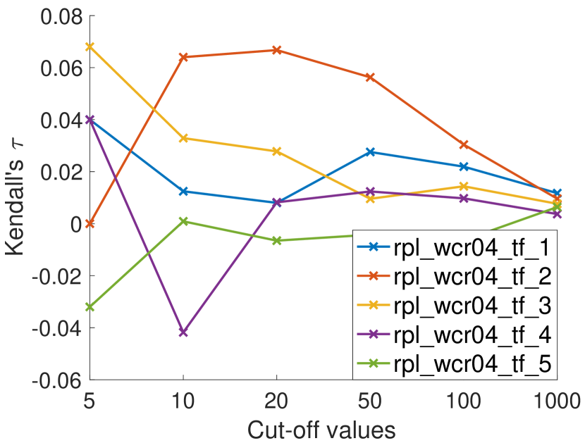
(a) Kendall’s $\tau$ WCrobust04.

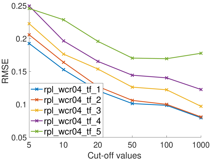
(b) RMSE WCrobust04.

Figure 1. Kendall’s $\tau$ and RMSE with nDCG computed at different cut-offs for WCrobust04.

Table 1 reports the retrieval performance for the baseline $b$-run WCrobust04 and the replicability measures: Kendall’s $\tau$, RBO, RMSE, and the $p$-values returned by the paired $t$-test. The corresponding table for WCrobust0405 reports similar results and is included in an online appendix . We report ER in Table 2 and plot ER against DeltaRI in Figure 2, additional ER-DeltaRI plots are included in the online appendix.

In Table  1, low values for Kendall’s $\tau$ and RBO highlights how hard it is to accurately replicate a run at ranking level. Replicability runs achieve higher RBO scores than Kendall’s $\tau$, showing that RBO is somehow less strict.

RMSE increases almost consistently when the difference between ARP scores of the original and replicated runs decreases. In general, RMSE values of P@10 are larger compared to those of AP and nDCG, due to P@10 having naturally higher variance (since it also considers a lower cut-off). For the constellation rpl_wcr04_tf and rpl_wcr04_C, RMSE with P@10 increases, even if the difference between ARP scores decreases. As pointed out in Section 3.1, this is due to RMSE which penalizes large errors. On the other hand, RMSE decreases almost consistently as the cut-off value increases, as shown in Figure 1(b). As expected, if we consider the whole ranking, the replicability runs retrieve more relevant documents and thus achieve better RMSE scores.

As a general observation, it is easier to replicate a run in terms of RMSE rather than Kendall’s $\tau$ or RBO. This is further corroborated by the correlation results in Table 4, which shows low correlation between RMSE and Kendall’s $\tau$. Therefore, even if the original and the replicated runs place documents with the same relevance labels in the same rank positions, those documents are not the same, as shown in Figure 1(a), where Kendall’s $\tau$ is computed at different cut-offs. This does not affect the system performance, but it might affect the user experience, which can be completely different.

For the paired $t$-test, as the difference in ARP decreases, $p$-value increases, showing that the runs are more similar. This is further validated by high correlation results reported in Table 4 between ARP and $p$-values. Recall that the numerator of the $t$-value is basically computing the difference in ARP scores, thus explaining the consistency of these results.

For rpl_wcr04_tf and rpl_wcr04_C, RMSE and $p$-values are not consistent: RMSE increases, thus the error increases, but $p$-values also increase, thus the runs are considered more similar. As aforementioned, this happens because RMSE penalizes large errors per topic, while the $t$-statistic is tightly related to ARP scores.

Table 2. ER results for replicability and reproducibility: the $a$-run is WCrobust0405 on TREC Common Core 2017; the $b$-run is WCrobust04, for replicability on TREC Common Core 2017, for reproducibility on TREC Common Core 2018.

	replicability			reproducibility
run	P@10	AP	nDCG	P@10	AP	nDCG
rpl_tf_1	$0.8077$	$1.0330$	$1.1724$	$1.1923$	$1.2724$	$2.0299$
rpl_tf_2	$0.7308$	$1.0347$	$1.1336$	$0.9615$	$1.3195$	$2.2139$
rpl_tf_3	$0.9038$	$1.3503$	$1.3751$	$1.5000$	$1.5616$	$2.5365$
rpl_tf_4	$0.6346$	$1.4719$	$1.5703$	$1.4231$	$1.9493$	$2.9317$
rpl_tf_5	$1.1346$	$1.5955$	$1.8221$	$1.5385$	$1.7010$	$3.0569$
rpl_df_1	$0.9615$	$0.9995$	$1.1006$	$0.4615$	$0.7033$	$0.9547$
rpl_df_2	$1.0192$	$0.9207$	$1.0656$	$0.4231$	$0.4934$	$0.6586$
rpl_df_3	$1.0385$	$0.8016$	$1.0137$	$0.1923$	$0.5429$	$1.0607$
rpl_df_4	$0.9615$	$0.5911$	$0.8747$	$0.3846$	$0.5136$	$0.8333$
rpl_df_5	$0.8654$	$0.3506$	$0.6459$	$0.3846$	$0.4857$	$0.7260$
rpl_tol_1	$1.0769$	$1.2013$	$1.3455$	$0.5769$	$0.6574$	$0.8780$
rpl_tol_2	$1.3269$	$1.4946$	$1.9290$	$0.8077$	$0.5194$	$0.8577$
rpl_tol_3	$1.8654$	$2.1485$	$2.8496$	$2.0000$	$1.4524$	$2.9193$
rpl_tol_4	$2.0962$	$2.2425$	$3.3213$	$2.3846$	$2.1242$	$3.9092$
rpl_tol_5	$1.2500$	$1.0469$	$1.8504$	$0.2692$	$0.1116$	$0.5595$
rpl_C_1	$0.6346$	$0.6300$	$0.8901$	$2.1538$	$1.8877$	$3.7777$
rpl_C_2	$0.8077$	$0.7361$	$0.9240$	$2.2308$	$1.9644$	$3.8621$
rpl_C_3	$0.8654$	$1.1195$	$1.2092$	$2.3846$	$2.2743$	$4.2783$
rpl_C_4	$0.9231$	$1.1642$	$1.2911$	$0.6538$	$0.7316$	$1.0403$
rpl_C_5	$0.8846$	$1.1214$	$1.2542$	$0.5769$	$0.6915$	$0.9741$

Table 2 (left) reports ER scores for replicability runs. WCrobust_04 is the baseline $b$-run, while WCrobust_0405 is the advanced $a$-run, both of them on TREC Common Core 2017. Recall that, for ER, the closer the score to $1$, the more successful the replication.

ER behaves as expected: when the quality of the replicated runs deteriorates, ER scores tend to move further from $1$. As for RMSE, we can observe that the extent of success for the replication experiments depends on the effectiveness measure. Thus, the best practice is to consider multiple effectiveness measures.

Note that, for the constellations of runs rpl_wcr04_tf and rpl_wcr04_C, there is no agreement among the best replication experiment when different effectiveness measures are considered. This trend is similar to the one observed with RMSE, $p$-values and delta in ARP. For example, for ER with P@10, the best replicability runs are rpl_wcr04_tf3 and rpl_wcr0405_tf3 but ER scores are not stable, while for AP and nDCG, ER values tends to move further from $1$, as we deteriorate the replicability runs. Again, this is due to the high variance of P@10.

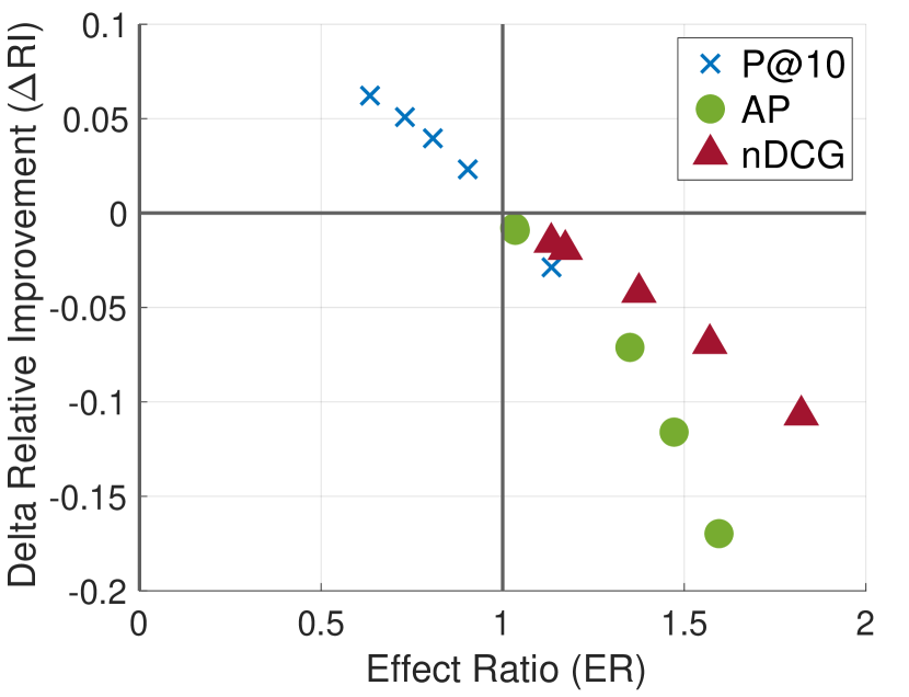
(a) rpl_tf runs.

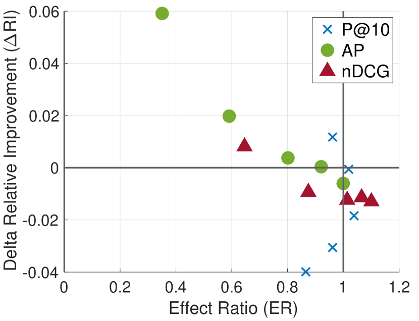
(b) rpl_df runs.

Figure 2. Replicability: ER on the $x$-axis against DeltaRI on the $y$-axis.

Figure 2 illustrates ER scores against DeltaRI for $2$ constellations in Table 2 and the other constellations are included in the online appendix. Recall that in Figure 2, the closer a point to the reference $(1,0)$, the better the replication experiment, both in terms of effect sizes and absolute differences.

The ER-DeltaRI plot, can be used as a visual tool to guide researcher on the exploration of the “space of replicability” runs. For example, in Figure  2(a), for AP and nDCG the point $(1,0)$ is reached from Region $4$, which is somehow the preferred region, since it corresponds to successful replication both in terms of effect sizes and relative improvements. Conversely, in Figure 2(b), it is clear that for AP the point $(1,0)$ is reached from Region $1$, which corresponds to somehow a successful replication in terms of effect sizes, but not in terms of relative improvements.

Case Study: Reproducibility

For reproducibility, Table 3 reports ARP and $p$-values in terms of P@10, AP, and nDCG, for the runs reproducing WCrobust04 on TREC Common Core 2018. The corresponding table for WCrobust0405 is included in the online appendix. Note that, in this case we do not have the original run scores, so we cannot directly compare ARP values. This represents the main challenge when evaluating reproducibility runs.

From $p$-values in Table 3, we can conclude that all the reproducibility runs are statistically significantly different from the original run, being the highest $p$-value just $0.005$. Therefore, it seems that none of the runs successfully reproduced the original run.

However, this is likely due to the two collections being too different, which in turn makes the scores distribution also different. Consequently the $t$-test considers all the distributions as significantly different. To validate this hypothesis, we carried out an unpaired $t$-test between pairs of replicability and reproducibility runs in the $4$ different constellations. This means that each pair of runs is generated by the same system on two different collections. The $p$-values for this experiment are reported only in the online appendix. Again, the majority of the runs are considered statistically differerent, except for a few cases for rpl_wcr04_df and rpl_wcr04_tol, which exhibit higher $p$-values also in Table 3. This shows that, depending on the collections, the unpaired $t$-test can fail in correctly detecting reproduced runs.

Table 2 (right) reports ER scores for replicability runs. At a first sight, we can see that ER scores are much lower (close to $0$) or much higher ($\gg 1$) than for the replicability case. If it is hard to perfectly replicate an experiment, it is even harder to perfectly reproduce it.

This is illustrated in the ER-DeltaRI plot in Figure 3. In Figure 3(a) the majority of the points are far from the best reproduction $(1,0)$, even if they are in region $4$. In Figure 3(b) just one point is in the preferred region $4$, while many points are in region $2$, that is failure both in reproducing the effect size and the relative improvement.

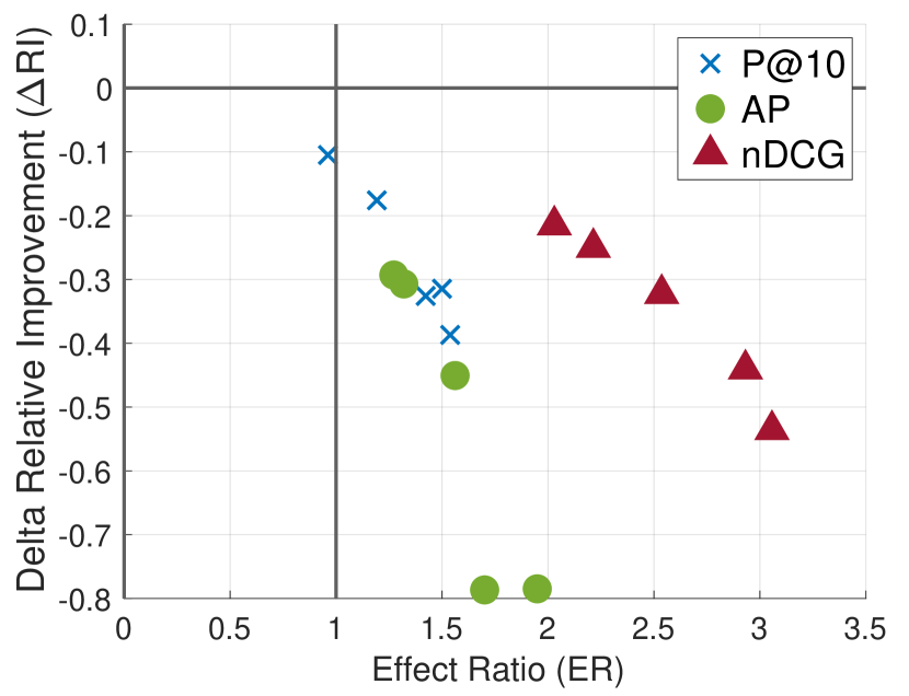
(a) rpd_tf runs.

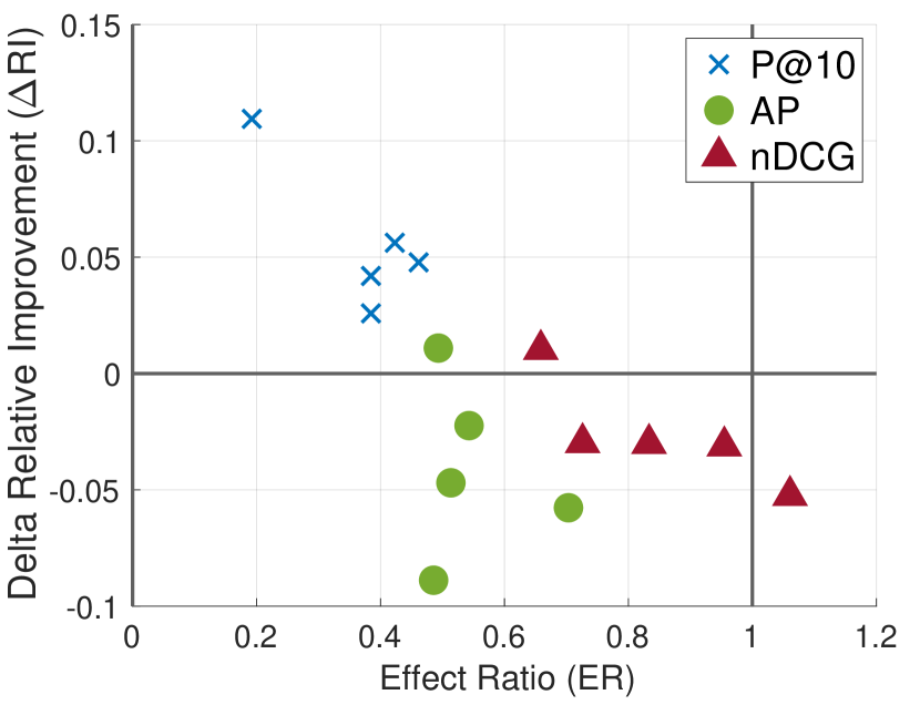
(b) rpd_df runs.

Figure 3. Reproducibility: ER on the $x$-axis against DeltaRI on the $y$-axis.

Table 3. Reproducibility: ARP and $p$-value (unpaired $t$-test), for WCrobust04. The original runs are on TREC Common Core 2017, and reproduced runs on TREC Common Core 2018.

	ARP			$p$-value
run	P@10	AP	nDCG	P@10	AP	nDCG
rpd_tf_1	$0.3680$	$0.1619$	$0.3876$	$7E{-}04$	$6E{-}06$	$6E{-}06$
rpd_tf_2	$0.3760$	$0.1628$	$0.3793$	$9E{-}04$	$8E{-}06$	$4E{-}06$
rpd_tf_3	$0.3280$	$0.1468$	$0.3587$	$8E{-}05$	$1E{-}06$	$8E{-}07$
rpd_tf_4	$0.3040$	$0.1180$	$0.3225$	$2E{-}05$	$3E{-}08$	$1E{-}08$
rpd_tf_5	$0.2920$	$0.1027$	$0.2854$	$1E{-}05$	$6E{-}09$	$4E{-}10$
rpd_df_1	$0.4240$	$0.1895$	$0.4543$	$0.005$	$8E{-}05$	$3E{-}04$
rpd_df_2	$0.4200$	$0.1972$	$0.4727$	$0.003$	$1E{-}04$	$9E{-}04$
rpd_df_3	$0.3880$	$0.1757$	$0.4304$	$0.001$	$2E{-}05$	$8E{-}05$
rpd_df_4	$0.3360$	$0.1458$	$0.4000$	$7E{-}05$	$8E{-}07$	$6E{-}06$
rpd_df_5	$0.2960$	$0.1140$	$0.3495$	$9E{-}06$	$1E{-}08$	$1E{-}07$
rpd_tol_1	$0.4200$	$0.1872$	$0.4469$	$0.005$	$6E{-}05$	$2E{-}04$
rpd_tol_2	$0.3960$	$0.1769$	$0.4134$	$0.002$	$3E{-}05$	$5E{-}05$
rpd_tol_3	$0.2040$	$0.0987$	$0.2365$	$7E{-}08$	$8E{-}09$	$1E{-}10$
rpd_tol_4	$0.0720$	$0.0183$	$0.0572$	$1E{-}12$	$5E{-}14$	$3E{-}22$
rpd_tol_5	$0.0200$	$0.0007$	$0.0048$	$5E{-}16$	$1E{-}15$	$3E{-}27$
rpd_C_1	$0.2600$	$0.1228$	$0.2786$	$5E{-}06$	$3E{-}07$	$2E{-}08$
rpd_C_2	$0.2600$	$0.1216$	$0.2790$	$5E{-}06$	$2E{-}07$	$2E{-}08$
rpd_C_3	$0.2360$	$0.0969$	$0.2507$	$8E{-}07$	$7E{-}09$	$5E{-}10$
rpd_C_4	$0.3600$	$0.1609$	$0.4095$	$3E{-}04$	$4E{-}06$	$1E{-}05$
rpd_C_5	$0.3520$	$0.1565$	$0.4026$	$2E{-}04$	$2E{-}06$	$8E{-}06$

5.2. Correlation Analysis

Replicability

Note that for some measures, namely Kendall’s $\tau$, RBO, $p$-value, the higher the score the better the replicated run, conversely for RMSE and Delta ARP (absolute difference in ARP), the lower the score the better the replicated run. Thus, before computing the correlation among measures, we ensure that all the measure scores are consistent with respect to each other. Practically we consider the opposite of $\tau$, RBO and $p$-values, and for ER we consider $|1-ER|$, since the closer its score to $1$, the better the replicability performance.

Table 4 reports Kendall’s $\tau$ correlation for replicability measures on the set of runs replicating WCrobust04 (upper triangle, white background) and WCrobust0405 (lower triangle, turquoise background). The correlation between ARP and $\tau$ is low, below $0.29$, and higher for RBO $0.70$. This validates the findings from Section 5.1, showing that Kendall’s $\tau$ assumes a totally different perspective when evaluating replicability runs. Between $\tau$ and RBO, RBO correlates more with ARP than $\tau$, especially with respect to AP and nDCG. Also, $\tau$ and RBO are low correlated with respect to each other. This is due to RBO being top-heavy, as AP and nDCG, while Kendall’s $\tau$ considers each rank position as equally important.

The correlation among ARP and RMSE is higher, especially when the same measure is considered by both ARP and RMSE. Nevertheless, the correlation is always lower than $0.86$, showing that it is different to compare the overall average or the performance score topic by topic, as also shown by P@10 in Table 1. Furthermore, the correlation between RMSE instantiated with AP and nDCG is high, above $0.9$, this is due to AP and nDCG being highly correlated, as also shown by the correlation between ARP with AP and nDCG (above $0.90$) and between $p$-values with AP and nDCG (above $0.91$).

When using the same performance measure, ARP and $p$-values approaches are highly correlated, even if from Table 1 several runs have small $p$-values and are statistically different. As mentioned in Section 5.1, the numerator of the $t$-stat is Delta ARP, and likely due to low variance, Delta ARP and $p$-values are tightly related.

As explained in Section 3.1, ER takes a different perspective when evaluating replicability runs. This is corroborated by correlation results, which show that this measure has low correlation with ARP and any other evaluation approach. Indeed, replicating the overall improvement over a baseline, does not mean that there is perfect replication on each topic. Moreover, even the correlation among ER instantiated with different measures is low, which means that a mean improvement over the baseline in terms of AP does not necessarily correspond to a similar mean improvement for nDCG.

Table 4. Replicability: correlation among different measures for runs replicating WCrobust04 (white background); and runs replicating WCrobust0405 (turquoise background).

	Delta ARP			Correlation		RMSE			$p$-value			ER
	P@10	AP	nDCG	$\tau$	RBO	P@10	AP	nDCG	P@10	AP	nDCG	P@10	AP	nDCG
$\Delta$arp_P@10	-	$0.4175$	$0.3979$	$0.2456$	$0.3684$	$0.3419$	$0.4552$	$0.4290$	$0.9156$	$0.3668$	$0.3700$	$0.2348$	$0.1752$	$0.0884$
$\Delta$arp_AP	$0.4535$	-	$0.9118$	$0.2718$	$0.7045$	$0.5209$	$0.8514$	$0.8090$	$0.3855$	$0.8841$	$0.8596$	$0.2145$	$0.3012$	$0.3731$
$\Delta$arp_nDCG	$0.4716$	$0.9363$	-	$0.2882$	$0.6555$	$0.5339$	$0.8580$	$0.8547$	$0.3463$	$0.8318$	$0.8302$	$0.2374$	$0.3208$	$0.4318$
$\tau$	$0.2620$	$0.2865$	$0.2620$	-	$0.2180$	$0.2788$	$0.2702$	$0.2898$	$0.2434$	$0.2376$	$0.2457$	$0.1834$	$0.2718$	$0.2098$
RBO	$0.3946$	$0.6637$	$0.6457$	$0.3584$	-	$0.6026$	$0.7616$	$0.6898$	$0.3201$	$0.6376$	$0.6490$	$0.3307$	$0.2049$	$0.3029$
RMSE_P@10	$0.5420$	$0.6713$	$0.7089$	$0.3213$	$0.7433$	-	$0.6239$	$0.5944$	$0.2544$	$0.4080$	$0.4129$	$0.3452$	$0.2706$	$0.3753$
RMSE_AP	$0.5076$	$0.7747$	$0.8188$	$0.3224$	$0.7910$	$0.8136$	-	$0.8988$	$0.4034$	$0.7355$	$0.7273$	$0.2734$	$0.3453$	$0.4171$
RMSE_nDCG	$0.4666$	$0.7616$	$0.8188$	$0.3094$	$0.7682$	$0.8054$	$0.9184$	-	$0.3806$	$0.7127$	$0.6849$	$0.2767$	$0.3649$	$0.4498$
p_value_P@10	$0.8393$	$0.3694$	$0.3645$	$0.2566$	$0.2877$	$0.3790$	$0.3743$	$0.3400$	-	$0.3740$	$0.3593$	$0.2129$	$0.1486$	$0.0327$
p_value_AP	$0.3913$	$0.8498$	$0.7927$	$0.2506$	$0.5657$	$0.5470$	$0.6245$	$0.6180$	$0.3564$	-	$0.9135$	$0.1736$	$0.2343$	$0.2898$
p_value_nDCG	$0.3848$	$0.8416$	$0.7845$	$0.2424$	$0.5543$	$0.5356$	$0.6196$	$0.6033$	$0.3384$	$0.9069$	-	$0.2178$	$0.2163$	$0.3110$
ER_P@10	$0.0739$	$0.2652$	$0.2767$	$0.2227$	$0.3537$	$0.3108$	$0.3193$	$0.3144$	$0.0459$	$0.1817$	$0.1867$	-	$0.2833$	$0.1736$
ER_AP	$0.3013$	$0.2963$	$0.3078$	$0.1673$	$0.2343$	$0.3312$	$0.3551$	$0.3420$	$0.2599$	$0.1886$	$0.1706$	$0.2833$	-	$0.3992$
ER_nDCG	$0.2718$	$0.2767$	$0.3143$	$0.1216$	$0.2669$	$0.3377$	$0.3747$	$0.3551$	$0.1553$	$0.1494$	$0.1706$	$0.1736$	$0.3992$	-

Reproducibility

Table 5. Reproducibility: correlation among different measures for runs reproducing WCrobust04 (white background); and runs reproducing WCrobust0405 (turquoise background).

	$p$-value			ER
	P@10	AP	nDCG	P@10	AP	nDCG
p_value_P@10	-	$0.8545$	$0.8446$	$-0.2050$	$-0.1153$	$0.0025$
p_value_AP	$0.8168$	-	$0.8694$	$-0.1743$	$-0.1151$	$-0.0335$
p_value_nDCG	$0.8054$	$0.9216$	-	$-0.2350$	$-0.2033$	$-0.0857$
ER_P@10	$0.0939$	$0.0674$	$0.0756$	-	$0.5651$	$0.3091$
ER_AP	$0.2232$	$0.2082$	$0.2473$	$0.5886$	-	$0.5298$
ER_nDCG	$0.1006$	$0.1167$	$0.1559$	$0.2220$	$0.4318$	-

For reproducibility we can not compare against ARP: since the original and reproduced runs are defined on different collections, it is meaningless to contrast average scores. Table 5 reports the correlation among reproducibility runs for WCrobust04 (upper triangle, white background) and for WCrobust0405 (lower triangle, turquoise background). Again, before computing the correlation among different measures, we ensured that the meaning of their scores is consistent across measures, i.e. the lower the score the better the reproduced results.

The correlation results for reproducibility show once more that ER is low correlated to $p$-values approaches, thus these methods are taking two different evaluation perspectives. Furthermore, ER has low correlation with itself when instantiated with different performance measures: even for reproducibility, two different performance measures do not exhibit an average improvement over baseline runs in a similar way.

Finally, all $p$-values approaches are fairly correlated with respect to each other, even stronger than in the replicability case of Table 4. This is surprising, if we consider that all the reproducibility runs are statistically significantly different, as shown in Table 3. However, it represents a further signal that the unpaired $t$-test is not able to recognise successfully reproduced runs, when the new collection and the original collection are too different, independently of the effectiveness measure.

6. Conclusions and Future Work

We faced the core issue of investigating measures to determine to what extent a system-oriented IR experiment has been replicated or reproduced. To this end, we analysed and compared several measures at different levels of granularity and we developed the first reproducibility-oriented dataset. Due to the lack of a reproducibility-oriented dataset, these measures have never been validated so far.

We found that replicability measures behave as expected and consistently; in particular, RBO provides more meaningfull comparisons than Kendall’s $\tau$; RMSE properly indicates whether we obtained a similar level of performance; finally, both ER/DeltaRI and the paired t-test successfully determine whether the same effects are replicated. On the other hand, quantifying reproducibility is more challenging and, while ER/DeltaRI are still able to provide sensible insights, the unpaired t-test seems to be too sensitive to the differences among the experimental collections.

As a suggestion to improve our community practices, it is important to always provide not only the source code but also the actual run, as to enable precise checking for replicability; luckily, this is already happening when we operate within evaluation campaigns which gather and make available runs by their participants.

In future work, we will explore more advanced statistical methods to quantify reproducibility in a reliable way. Moreover, we will investigate how replicability and reproducibility are related to user experience. For example, a perfectly replicated run in terms of RMSE, but with low RBO, presents different documents to a user and this might greatly affect her/his experience. Therefore, we need to better understand which replicability/reproducibility level is needed to not impact (too much) on the user experience.

Acknowledgments. This paper is partially supported by AMAOS (Advanced Machine Learning for Automatic Omni-Channel Support), funded by Innovationsfonden, Denmark, and by DFG (German Research Foundation, project no. 407518790).

References

- (1)
- Allan et al. (2018) J. Allan, D. K. Harman, E. Kanoulas, D. Li, C. Van Gysel, and E. M. Voorhees. 2018. TREC 2017 Common Core Track Overview. In The Twenty-Sixth Text REtrieval Conference Proceedings (TREC 2017), E. M. Voorhees and A. Ellis (Eds.). National Institute of Standards and Technology (NIST), Special Publication 500-324, Washington, USA.
- Arguello et al. (2015) J. Arguello, M. Crane, F. Diaz, J. Lin, and A. Trotman. 2015. Report on the SIGIR 2015 Workshop on Reproducibility, Inexplicability, and Generalizability of Results (RIGOR). SIGIR Forum 49, 2 (December 2015), 107–116.
- Baker (2016) M. Baker. 2016. 1,500 Scientists Lift the Lid on Reproducibility. Nature 533 (May 2016), 452–454.
- Breuer et al. (2020) T. Breuer, N. Ferro, N. Fuhr, M. Maistro, T. Sakai, P. Schaer, and I. Soboroff. 2020. How to Measure the Reproducibility of System-oriented IR Experiments. https://doi.org/10.5281/zenodo.3856042
- Breuer and Schaer (2019) T. Breuer and P. Schaer. 2019. Replicability and Reproducibility of Automatic Routing Runs. In Working Notes of CLEF 2019 - Conference and Labs of the Evaluation Forum, Lugano, Switzerland, September 9-12, 2019 (CEUR Workshop Proceedings), Linda Cappellato, Nicola Ferro, David E. Losada, and Henning Müller (Eds.), Vol. 2380. CEUR-WS.org. http://ceur-ws.org/Vol-2380/paper_84.pdf
- Chua et al. (2008) T.-S. Chua, M.-K. Leong, D. W. Oard, and F. Sebastiani (Eds.). 2008. Proc. 31st Annual International ACM SIGIR Conference on Research and Development in Information Retrieval (SIGIR 2008). ACM Press, New York, USA.
- Clancy et al. (2019) R. Clancy, N. Ferro, C. Hauff, T. Sakai, and Z. Z. Wu. 2019. Overview of the 2019 Open-Source IR Replicability Challenge (OSIRRC 2019). In Proc. of the Open-Source IR Replicability Challenge (OSIRRC 2019), R. Clancy, N. Ferro, C. Hauff, T. Sakai, and Z. Z. Wu (Eds.). CEUR Workshop Proceedings (CEUR-WS.org), ISSN 1613-0073, http://ceur-ws.org/Vol-2409/, 1–7.
- Crane (2018) M. Crane. 2018. Questionable Answers in Question Answering Research: Reproducibility and Variability of Published Results. Transactions of the Association for Computational Linguistics (TACL) 6 (2018), 241–252.
- Croux and Dehon (2010) C. Croux and C. Dehon. 2010. Influence Functions of the Spearman and Kendall Correlation Measures. Statistical Methods & Applications 19 (2010), 497–515.
- Dacrema et al. (2019) M. F. Dacrema, P. Cremonesi, and D. Jannach. 2019. Are We Really Making Much Progress? A Worrying Analysis of Recent Neural Recommendation Approaches. In Proc. 13th ACM Conference on Recommender Systems, (RecSys 2019), T. Bogers, A. Said, P. Brusilovsky, and D. Tikk (Eds.). ACM Press, New York, USA, 101–109.
- De Roure (2014) D. De Roure. 2014. The Future of Scholarly Communications. Insights 27, 3 (November 2014), 233–238.
- Ferrante et al. (2015) M. Ferrante, N. Ferro, and M. Maistro. 2015. Towards a Formal Framework for Utility-oriented Measurements of Retrieval Effectiveness. In Proc. 1st ACM SIGIR International Conference on the Theory of Information Retrieval (ICTIR 2015), J. Allan, W. B. Croft, A. P. de Vries, C. Zhai, N. Fuhr, and Y. Zhang (Eds.). ACM Press, New York, USA, 21–30.
- Ferro (2017) N. Ferro. 2017. What Does Affect the Correlation Among Evaluation Measures? ACM Transactions on Information Systems (TOIS) 36, 2 (September 2017), 19:1–19:40.
- Ferro et al. (2019) N. Ferro, N. Fuhr, M. Maistro, T. Sakai, and I. Soboroff. 2019. Overview of CENTRE@CLEF 2019: Sequel in the Systematic Reproducibility Realm. In Experimental IR Meets Multilinguality, Multimodality, and Interaction. Proceedings of the Tenth International Conference of the CLEF Association (CLEF 2019), F. Crestani, M. Braschler, J. Savoy, A. Rauber, H. Müller, D. E. Losada, G. Heinatz Bürki, L. Cappellato, and N. Ferro (Eds.). Lecture Notes in Computer Science (LNCS) 11696, Springer, Heidelberg, Germany, 287–300.
- Ferro et al. (2018a) N. Ferro, N. Fuhr, and A. Rauber. 2018a. Introduction to the Special Issue on Reproducibility in Information Retrieval: Evaluation Campaigns, Collections, and Analyses. ACM Journal of Data and Information Quality (JDIQ) 10, 3 (October 2018), 9:1–9:4.
- Ferro et al. (2018b) N. Ferro, N. Fuhr, and A. Rauber. 2018b. Introduction to the Special Issue on Reproducibility in Information Retrieval: Tools and Infrastructures. ACM Journal of Data and Information Quality (JDIQ) 10, 4 (November 2018), 14:1–14:4.
- Ferro and Kelly (2018) N. Ferro and D. Kelly. 2018. SIGIR Initiative to Implement ACM Artifact Review and Badging. SIGIR Forum 52, 1 (June 2018), 4–10.
- Ferro et al. (2018c) N. Ferro, M. Maistro, T. Sakai, and I. Soboroff. 2018c. Overview of CENTRE@CLEF 2018: a First Tale in the Systematic Reproducibility Realm. In Experimental IR Meets Multilinguality, Multimodality, and Interaction. Proceedings of the Nineth International Conference of the CLEF Association (CLEF 2018), P. Bellot, C. Trabelsi, J. Mothe, F. Murtagh, J.-Y. Nie, L. Soulier, E. SanJuan, L. Cappellato, and N. Ferro (Eds.). Lecture Notes in Computer Science (LNCS) 11018, Springer, Heidelberg, Germany, 239–246.
- Freire et al. (2016) J. Freire, N. Fuhr, and A. Rauber (Eds.). 2016. Report from Dagstuhl Seminar 16041: Reproducibility of Data-Oriented Experiments in e-Science. Schloss Dagstuhl–Leibniz-Zentrum für Informatik, Germany.
- Fuhr (2017) N. Fuhr. 2017. Some Common Mistakes In IR Evaluation, And How They Can Be Avoided. SIGIR Forum 51, 3 (December 2017), 32–41.
- Fuhr (2019) N. Fuhr. 2019. Reproducibility and Validity in CLEF. In Information Retrieval Evaluation in a Changing World – Lessons Learned from 20 Years of CLEF (The Information Retrieval Series), N. Ferro and C. Peters (Eds.), Vol. 41. Springer International Publishing, Germany.
- Gibney (2020) E. Gibney. 2020. This AI researcher is trying to ward off a reproducibility crisis. Nature 577 (January 2020), 14.
- Grossman and Cormack (2017) Maura R. Grossman and Gordon V. Cormack. 2017. MRG_UWaterloo and WaterlooCormack Participation in the TREC 2017 Common Core Track. In Proceedings of The Twenty-Sixth Text REtrieval Conference, TREC 2017, Gaithersburg, Maryland, USA, November 15-17, 2017, Ellen M. Voorhees and Angela Ellis (Eds.), Vol. Special Publication 500-324. National Institute of Standards and Technology (NIST). https://trec.nist.gov/pubs/trec26/papers/MRG_UWaterloo-CC.pdf
- ISO 5725-2:2019 (2019) ISO 5725-2:2019. 2019. Accuracy (Trueness and Precision) of Measurement Methods and Results – Part 2: Basic Method for the Determination of Repeatability and Reproducibility of a Standard Measurement method. Recommendation ISO/IEC 5725-2:2019.
- Kendall (1948) M. G. Kendall. 1948. Rank correlation methods. Griffin, Oxford, England.
- Kenney and Keeping (1954) J. F. Kenney and E. S. Keeping. 1954. Mathematics of Statistics – Part One (3rd ed.). D. Van Nostrand Company, Princeton, USA.
- Lin et al. (2016) J. Lin, M. Crane, A. Trotman, J. Callan, I. Chattopadhyaya, J. Foley, G. Ingersoll, C. Macdonald, and S. Vigna. 2016. Toward Reproducible Baselines: The Open-Source IR Reproducibility Challenge. In Advances in Information Retrieval. Proc. 38th European Conference on IR Research (ECIR 2016), N. Ferro, F. Crestani, M.-F. Moens, J. Mothe, F. Silvestri, G. M. Di Nunzio, C. Hauff, and G. Silvello (Eds.). Lecture Notes in Computer Science (LNCS) 9626, Springer, Heidelberg, Germany, 357–368.
- National Academies of Sciences, Engineering, and Medicine (2016) National Academies of Sciences, Engineering, and Medicine. 2016. Statistical Challenges in Assessing and Fostering the Reproducibility of Scientific Results: Summary of a Workshop. The National Academies Press, Washington, USA.
- National Academies of Sciences, Engineering, and Medicine (2019) National Academies of Sciences, Engineering, and Medicine. 2019. Reproducibility and Replicability in Science. The National Academies Press, Washington, USA.
- Open Science Collaboration (2015) Open Science Collaboration. 2015. Estimating the Reproducibility of Psychological Science. Science 349, 6251 (August 2015), 943–952.
- Plesser (2018) H. E. Plesser. 2018. Reproducibility vs. Replicability: A Brief History of a Confused Terminology. Frontiers in Neuroinformatics 11 (January 2018), 76:1–76:4.
- Robertson and Callan (2005) S. Robertson and J. Callan. 2005. Routing and Filtering. In TREC: Experiment and Evaluation in Information Retrieval, E. M. Voorhees and D. K. Harman (Eds.). MIT Press, Cambridge, Massachusetts, 99–122.
- Sakai (2016) T. Sakai. 2016. Two Sample T-tests for IR Evaluation: Student or Welch?. In Proc. 39th Annual International ACM SIGIR Conference on Research and Development in Information Retrieval (SIGIR 2016), R. Perego, F. Sebastiani, J. Aslam, I. Ruthven, and J. Zobel (Eds.). ACM Press, New York, USA, 1045–1048.
- Sakai (2018) T. Sakai. 2018. Laboratory Experiments in Information Retrieval. The Information Retrieval Series, Vol. 40. Springer Singapore.
- Sakai et al. (2019) T. Sakai, N. Ferro, I. Soboroff, Z. Zeng, P. Xiao, and M. Maistro. 2019. Overview of the NTCIR-14 CENTRE Task. In Proc. 14th NTCIR Conference on Evaluation of Information Access Technologies, E. Ishita, N. Kando, M. P. Kato, and Y. Liu (Eds.). National Institute of Informatics, Tokyo, Japan, 494–509.
- Sanderson and Soboroff (2007) M. Sanderson and I. Soboroff. 2007. Problems with Kendall’s Tau. In Proc. 30th Annual International ACM SIGIR Conference on Research and Development in Information Retrieval (SIGIR 2007), W. Kraaij, A. P. de Vries, C. L. A. Clarke, N. Fuhr, and N. Kando (Eds.). ACM Press, New York, USA, 839–840.
- Soboroff et al. (2019) I. Soboroff, N. Ferro, M. Maistro, and T. Sakai. 2019. Overview of the TREC 2018 CENTRE Track. In The Twenty-Seventh Text REtrieval Conference Proceedings (TREC 2018), E. M. Voorhees and A. Ellis (Eds.). National Institute of Standards and Technology (NIST), Special Publication 500-331, Washington, USA.
- Student (1908) Student. 1908. The Probable Error of a Mean. Biometrika 6, 1 (March 1908), 1–25.
- Voorhees (1998) E. M. Voorhees. 1998. Variations in Relevance Judgments and the Measurement of Retrieval Effectiveness. In Proc. 21st Annual International ACM SIGIR Conference on Research and Development in Information Retrieval (SIGIR 1998), W. B. Croft, A. Moffat, C. J. van Rijsbergen, R. Wilkinson, and J. Zobel (Eds.). ACM Press, New York, USA, 315–323.
- Webber et al. (2010) W. Webber, A. Moffat, and J. Zobel. 2010. A Similarity Measure for Indefinite Rankings. ACM Transactions on Information Systems (TOIS) 4, 28 (November 2010), 20:1–20:38.
- Webber et al. (2008) W. Webber, A. Moffat, J. Zobel, and T. Sakai. 2008. Precision-at-ten Considered Redundant, See Chua et al. (2008), 695–696.
- Yilmaz et al. (2008) E. Yilmaz, J. A. Aslam, and S. E. Robertson. 2008. A New Rank Correlation Coefficient for Information Retrieval, See Chua et al. (2008), 587–594.