Generation and storage of spin squeezing via learning-assisted optimal control

Abstract

The generation and storage of spin squeezing is an attractive topic in quantum metrology and the foundations of quantum mechanics. The major models to realize the spin squeezing are the one- and two-axis twisting models. Here, we consider a collective spin system coupled to a bosonic field, and show that proper constant-value controls in this model can simulate the dynamical behavior of these two models. More interestingly, a better performance of squeezing can be obtained when the control is time-varying, which is generated via a reinforcement learning algorithm. However, this advantage becomes limited if the collective noise is involved. To deal with it, we propose a four-step strategy for the construction of a new type of combined controls, which include both constant-value and time-varying controls, but performed at different time intervals. Compared to the full time-varying controls, the combined controls not only give a comparable minimum value of the squeezing parameter over time, but also provides a better lifetime and larger full amount of squeezing. Moreover, the amplitude form of a combined control is simpler and more stable than the full time-varying control. Therefore, our scheme is very promising to be applied in practice to improve the generation and storage performance of squeezing.

I introduction

Many advantages of quantum technology require the assistance of quantum resources. Squeezing is such a resource Yuen1976 ; Walls1994 ; Scully1997 . Consider a pair of canonical observables $X$ and $Y$. Their deviations $\Delta X$ and $\Delta Y$ in a system satisfy the Heisenberg uncertainty relation $\Delta X\Delta Y\geq|\langle[X,Y]\rangle|/2$. The system is called squeezed when one of the deviations is less than the square root of the bound above. A typical example is the squeezed vacuum state, in which the deviation of the quadrature operator is squeezed. The squeezed light has been proved to be very useful in many aspects of quantum information, especially in quantum metrology Caves1981 ; Lang2013 , and it is now a promising candidate to be applied in the next-generation gravitational-wave observatory on earth for the further improvement of the detection sensitivity Grote2013 . Apart from the light, the atoms can also present squeezing behaviors, known as the spin squeezing Kitagawa1993 ; Wineland1992 ; Wineland1994 ; Ma2011 ; Pezze2018 ; Cronin2009 ; Sau2010 ; Vitagliano2011 . Similar to the squeezed light, the squeezed atoms can also improve the measurement precision beyond the standard quantum limit Ma2011 ; Pezze2018 , and more interestingly, witness the many-body entanglement Guehne2009 .

In the early 1990th, two types of squeezing parameters for the quantification of spin squeezing were provided by Kitagawa and Ueda Kitagawa1993 , and Wineland et al. Wineland1992 ; Wineland1994 . Kitagawa and Ueda Kitagawa1993 further proposed two different mechanisms, one- and two-axis twisting models, for the generation of spin squeezed states. The one-axis twisting (OAT) model Jin2009 ; Jin2007 ; Bennett2013 ; Zhong2014 ; Gross2010 ; Riedel2010 can provide a precision limit at the scaling $N^{-2/3}$ ($N$ is the particle number) and the two-axis twisting (TAT) model Helmerson2001 ; Zhang2003 ; Ng2003 ; Liu2011 ; Thomsen2002 ; Zhangyc2017 ; Groszkowski2020 ; Qin2020 provides a better scaling $N^{-1}$. These advantages motivate the scientists to try to realize these models in experiments. Currently, the OAT model can be readily obtained with the two-component Bose-Einstein condensate Gross2010 ; Riedel2010 or the nitrogen-vacancy centers Bennett2013 , yet the TAT model is more difficult to realize in practice. Several theoretical schemes have been proposed in recent years, such as utilizing the Raman processes Helmerson2001 ; Zhang2003 of Bose-Einstein condensate or the double well Ng2003 , converting the OAT model into an effective TAT model Liu2011 , phase-locked coupling between atoms and photons Zhangyc2017 , bosonic parametric driving Groszkowski2020 , employing feedback in the measurement system Thomsen2002 , and even using the week squeezing of light Qin2020 , Finding simple and experimental-friendly realizations of the TAT model and searching ways to go beyond it for the generation of squeezing are still the major concerns in this field.

In this paper, we consider a general collective spin system coupled to a bosonic field via the dispersive coupling, and propose an optimal control method for the generation and storage of spin squeezing. Both the constant-value and time-varying controls are studied with and without noise. The OAT and TAT models can be readily simulated by this system via proper constant-value controls. The time-varying controls are generated via the Deep Deterministic Policy Gradient (DDPG) algorithm Lillicrap2015 , an advanced reinforcement learning algorithm. In recent years, various machine learning algorithms Mohri2018 ; Hafner2011 ; Kevine2020 have been applied in many topics of quantum physics Carleo2019 ; Krenn2020 , such as quantum phase transitions Nieuwenburg2017 ; Nieuwenburg2018 ; Che2020 , quantum parameter estimation Xu2019 ; Hentschel2010 ; Hentschel2011 , quantum speed limits Zhang2018 , Hamiltonian learning Wang2017 and multipartite entanglement Krenn2016 ; Melnikov2018 ; Krenn2020 . Aided by the deep reinforcement learning, Chen et al. Chen2019 recently proposed a scheme in the OAT-type model with few discrete pulses, which can obtain an enhanced amount of squeezing close to the TAT model. In the collective spin system we consider, with the help of time-varying controls generated by the DDPG algorithm, the performance of squeezing goes significantly beyond the TAT model.

In practice, the collective spin system could be easily affected by the collective noise, and it is unfortunate that the advantage of time-varying controls becomes limited when this noise is involved. To deal with it, we propose a four-step strategy to generate a new type of combined controls, which include both constant-value and time-varying controls, but performed at different time intervals. The combined controls not only provide a similar maximum squeezing compared to both the constant-value and time-varying controls, but also significantly extend the lifetime and improve the full amount of squeezing over time. Due to the fact that the combined controls are simpler and more stable than the full time-varying controls, it is very promising to be applied in practical environment for the realization of an improved performance than the TAT model on the generation and storage of squeezing.

II physical model and spin squeezing

We consider a coupled atom-field system in which an ensemble of the two-level systems is coupled to a single-mode bosonic field. The Hamiltonian of this system reads

$$H_{0}=\omega_{c}a^{\dagger}a+\omega_{z}J_{z}+gJ_{x}(a^{\dagger}+a),$$ (1)

where $a$ $(a^{\dagger})$ is the annihilation (creation) operator of the field, which can be realized by a cavity, and $J_{m}=\sum^{N}_{i=1}\frac{1}{2}\sigma^{(i)}_{m}$ is the collective angular momentum operator with $N$ the particle number and $\sigma^{(i)}_{m}$ ($m=x,y,z$) the Pauli matrix for the $i$th spin. $\omega_{c}$ and $\omega_{z}$ are the frequencies of the field and collective system, respectively, and $g$ is the strength of the coupling. To help to generate spin squeezing, we invoke the quantum control via the time-dependent modulation field with the Hamiltonian

$$H_{\mathrm{c}}(t)=\zeta(t)\nu\cos(\nu t)J_{z},$$ (2)

where $\nu$ is the modulation frequency, $\zeta(t)$ is the amplitude. The model described by Eq. (1) can be realized with an ensemble of ⁸⁷Rb atoms with up state $|\!\!\uparrow\rangle:=|5^{2}S_{1/2},F=2,m_{F}=1\rangle$ and down state $|\!\!\downarrow\rangle:=|5^{2}S_{1/2},F=1,m_{F}=1\rangle$ coupled to a microwave cavity mode. The energy split between the hyperfine levels $|\!\!\uparrow\rangle$ and $|\!\!\downarrow\rangle$ is about 6.8GHz without magnetic field. In the presence of magnetic field, the Zeeman or hyperfine Paschen-Back shift has the same magnitude but opposite sign for the two hyperfine manifolds with $g_{F=2}=1/2$ and $g_{F=1}=-1/2$ Steck2019 . Thus, the modulation Hamiltonian $H_{c}(t)$ can be realized with a controllable magnetic field.

Due to the existence of noise on both the cavity and collective spin, the evolution of the total density matrix $\rho$ for our model is governed by the master equation

$$\partial_{t}\rho = -i\left[H_{0}+H_{\mathrm{c}},\rho\right]+\kappa\left(2a\rho a^{\dagger}-a^{\dagger}a\rho-\rho a^{\dagger}a\right)$$ (3)

$$+\gamma\left(2J_{z}\rho J_{z}-J_{z}^{2}\rho-\rho J_{z}^{2}\right)$$

with $\kappa$ and $\gamma$ being the cavity loss rate and atoms dephasing rate, respectively.

To characterize the degree of spin squeezing generated in this system, we use the squeezing parameter introduced by Kitagawa and Ueda Kitagawa1993

$$\xi^{2}=\frac{4}{N}(\Delta J_{n_{\bot}}^{2})_{\min},$$ (4)

where $(\Delta J_{n_{\bot}}^{2})_{{\min}}$ is the minimum variance in a direction vertical to the mean spin direction $\vec{n}_{0}$. A state is squeezed if $\xi^{2}<1$, and smaller $\xi^{2}$ indicates stronger squeezing. $\vec{n}_{0}$ in spherical coordinates is of the form $(\sin\theta\cos\phi,\sin\theta\sin\phi,\cos\theta)$, where $\theta=\arccos\left(\langle J_{z}\rangle/\sqrt{\langle J_{x}\rangle^{2}+\langle J_{y}\rangle^{2}+\langle J_{z}\rangle^{2}}\right)$ and $\phi=\arccos\left({\langle J_{x}\rangle}/{\sqrt{\langle J_{x}\rangle^{2}+\langle J_{y}\rangle^{2}}}\right)$ are polar and azimuthal angles, respectively. The other two orthogonal vectors with respect to $\vec{n}_{0}$ are $\vec{n}_{1}=(-\sin\phi,\cos\phi,0)$ and $\vec{n}_{2}=(-\cos\theta\cos\phi,-\cos\theta\sin\phi,\sin\theta)$. Define $J_{\vec{n}}=\vec{n}\cdot\vec{J}$ with $\vec{J}=(J_{x},J_{y},J_{z})$, the variance $(\Delta J_{n_{\bot}}^{2})_{{\rm min}}$ can be calculated via the equation

$$(\Delta J_{n_{\bot}}^{2})_{{\rm min}}=\frac{1}{2}\left(\mathcal{C}-\sqrt{\mathcal{A}^{2}+\mathcal{B}^{2}}\right),$$ (5)

where $\mathcal{C}=\langle J_{\vec{n}_{1}}^{2}+J_{\vec{n}_{2}}^{2}\rangle$, $\mathcal{A}=\langle J_{\vec{n}_{1}}^{2}-J_{\vec{n}_{2}}^{2}\rangle$, and $\mathcal{B}=\langle J_{\vec{n}_{1}}J_{\vec{n}_{2}}+J_{\vec{n}_{2}}J_{\vec{n}_{1}}\rangle$. Then the squeezing parameter becomes

$$\xi^{2}=\frac{2}{N}\left(\mathcal{C}-\sqrt{\mathcal{A}^{2}+\mathcal{B}^{2}}\right).$$ (6)

The corresponding optimal squeezing direction is

$$\vec{n}_{\mathrm{opt}}=\vec{n}_{1}\cos\left(\varphi_{\mathrm{opt}}\right)+\vec{n}_{2}\sin\left(\varphi_{\mathrm{opt}}\right),$$ (7)

where the optimal angle $\varphi_{\mathrm{opt}}$ reads Ma2011

$$\varphi_{\mathrm{opt}}=\begin{cases}\frac{1}{2}\arccos\left(\frac{-\mathcal{A}}{\sqrt{\mathcal{A}^{2}+\mathcal{B}^{2}}}\right),~{}\mathrm{for}~{}\mathcal{B}\leq 0,\\ \pi-\frac{1}{2}\arccos\left(\frac{-\mathcal{A}}{\sqrt{\mathcal{A}^{2}+\mathcal{B}^{2}}}\right),~{}\mathrm{for}~{}\mathcal{B}>0.\end{cases}$$ (8)

In our scheme, we assume that the ensemble of atoms is prepared in a coherent spin state, which is defined as

$$\left|\eta\right\rangle=(1+\left|\eta\right|^{2})^{-J}\sum_{m=-J}^{J}\left(\begin{array}[]{c}2J\\ J+m\end{array}\right)^{1/2}\eta^{J+m}\left|J,m\right\rangle,$$ (9)

where $\left|J,m\right\rangle$ ($J=N/2$, $m=0,\pm 1,\cdots,\pm J$ for an even $N$ and $\pm\frac{1}{2},\cdots,\pm J$ for an odd $N$) is known as the Dicke state, namely, the eigenstate of $J_{z}$ with eigenvalue $m$. Since $\eta$ can be expressed by $\eta=-\tan(\frac{\theta}{2})\exp(-i\phi)$, the coherent spin state can also be written as $|\theta,\phi\rangle$. In the following, the initial state of the atoms are taken as the coherent spin state $\left|\frac{\pi}{2},\frac{\pi}{2}\right\rangle$ and the initial state of the cavity is the vacuum state.

III Control-enhanced spin squeezing

III.1 Constant-value control

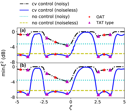
Figure 1: The minimum value of $\xi^{2}$ ($\min\,\xi^{2}$) as a function of $\zeta$ in the case of (a) $N=6$ and (b) $N=8$ for both noise and noiseless scenarios. The dash-dotted black and solid blue lines represent $\min\,\xi^{2}$ for the constant-value (cv) controls with and without noise. The dotted cyan and dashed yellow lines represent $\min\,\xi^{2}$ in the non-controlled scenario with and without noise. The values of $\min\,\xi^{2}$ for the effective OAT and TAT-type Hamiltonians are shown as the red stars and purple triangles. The decay rates are set to be $\kappa=\gamma=0.01g$ in the plots.

The constant-value control refers to invoking a time-independent value of control amplitude, i.e., $\zeta(t)=c$. This control is simple, economic and easy to be implemented in experiments. The Hamiltonian in Eq. (1) with a proper constant-value control can simulate a OAT or TAT-type Hamiltonian. In the rotating frame defined by $V(t)=\mathcal{T}\exp\left[i\int_{0}^{t}(H_{0}+H_{\mathrm{c}})d\tau\right]$ ($\mathcal{T}$ is the time-ordering operator), the Hamiltonian can be approximately rewritten into

$$\tilde{H}\approx(g_{0}J_{+}ae^{-i\delta t}+g_{m_{0}}J_{-}ae^{-i\Delta_{m_{0}}t})+\mathrm{H.c.},$$ (10)

when the condition $\nu\gg g,\delta$ is satisfied. Here $J_{\pm}=J_{x}\pm iJ_{y}$, $g_{0}=g\mathcal{J}_{0}(\zeta)/2$, $g_{m_{0}}=g\mathcal{J}_{m_{0}}(\zeta)/2$, $\delta=\omega_{c}-\omega_{z}$, and $\Delta_{m_{0}}=m_{0}\nu+\omega_{c}+\omega_{z}$ where $m_{0}$ is the optimal integer $m$ to reach the minimum value of $|m\nu+\omega_{c}+\omega_{z}|$. $\mathcal{J}_{n}(\zeta)$ is the $n$th Bessel function of the first kind. H.c. represents the Hermitian conjugate. In the case that $\delta=\Delta_{m_{0}}\equiv\Delta$, namely, $m_{0}=-2[\omega_{z}/\nu]$ ($[\cdot]$ is the rounding function), and rotating $\tilde{H}$ back to a non-rotating frame with $V_{1}=\exp(i\Delta a^{\dagger}at)$, an effective Hamiltonian $H_{1}=\Delta a^{\dagger}a+g(\Sigma^{\dagger}a+\Sigma a^{\dagger})$ can be obtained with $\Sigma=[\mathcal{J}_{0}(\zeta){J}_{-}+\mathcal{J}_{m_{0}}(\zeta){J}_{+}]/2$.

For large detunings $\Delta\gg g>g_{0}\,(g_{m_{0}})$, taking the transformation $e^{R}H_{1}e^{-R}$ with $R=\frac{g}{\Delta}(\Sigma a^{\dagger}-\Sigma^{\dagger}a)$, and truncating to the second order of $g/\Delta$, the effective Hamiltonian becomes (the details can be found in the Appendix)

$$H_{\rm eff} = \Delta a^{\dagger}a-\frac{g_{0}^{2}-g_{m_{0}}^{2}}{\Delta}(1+2a^{\dagger}a)J_{z}$$ (11)

$$+\frac{\left(g_{0}-g_{m_{0}}\right)^{2}}{\Delta}J_{z}^{2}-\frac{4g_{0}g_{m_{0}}}{\Delta}J_{x}^{2}.$$

An effective OAT model $\chi J_{x}^{2}$ can be obtained by the equation above when taking $g_{0}=g_{m_{0}}$ and the coefficient $\chi=-g^{2}\mathcal{J}_{m_{0}}^{2}(\zeta)/\Delta$. It is easy to see that when no control is involved ($\zeta=0$), the transformed Hamiltonian is also an OAT-type (with linear term) model Bennett2013 since $\mathcal{J}_{0}(0)=1$ and $\mathcal{J}_{m\neq 0}(0)=0$. Some values for $\zeta$ to simulate the OAT model are $-4.680,-1.435$, and $3.113$ for $m_{0}=-1$. Moreover, Eq. (11) can also simulate the TAT-type model

$$H_{\rm TAT-type}=-\lambda(J_{x}^{2}-J_{z}^{2})-\lambda^{\prime}(1+2a^{\dagger}a)J_{z},$$ (12)

when the coefficients satisfying $(g_{0}-g_{m_{0}})^{2}=4g_{0}g_{m_{0}}$, and the coefficients $\lambda=4g_{0}g_{m_{0}}/\Delta$ and $\lambda^{\prime}=(g_{0}^{2}-g_{m_{0}}^{2})/\Delta$. Some values for $\zeta$ to satisfy this condition are $-2.284,-0.338$, and $2.569$ for $m_{0}=-1$. The linear term can be eliminated on average through a dynamical decoupling protocol, which makes the transformed Hamiltonian a standard TAT Hamiltonian. The validity of this effective Hamiltonian are checked by calculating the fidelity between the evolved states given by the original and effective Hamiltonians, which is shown in the Appendix.

Apart from simulating the OAT and TAT models, searching ways to go beyond these models on the generation of squeezing is also crucial. Hence, the performance of a general constant-value control is studied for both noisy and noiseless scenarios, as shown in Fig. 1(a) for $N=6$ and Fig. 1(b) for $N=8$. The parameters are set as $w_{z}=110,w_{c}=100,\nu=200$ and $g=1$. In the noiseless scenario, the minimum values of $\xi^{2}(t)$ (solid blue lines, denoted by $\min\xi^{2}$), show a large amplitude waving behavior when the control amplitude $\zeta$ varies, and not all the values are capable to provide an enhanced squeezing than the non-controlled one ($\zeta=0$, dashed yellow lines). The TAT-type Hamiltonians provide a good squeezing performance (purple triangles) in the regime ([-5,5]) given in the plot. The corresponding values of $\min\xi^{2}$ are very close to the optimal ones. For a larger regime (for example [-10, 10]), the optimal values of $\zeta$ can provide a better performance than the TAT-type Hamiltonians, yet they may also have to face the difficulty of generation in practice. The OAT Hamiltonians (red stars) do not present an obvious advantage on squeezing than the non-controlled one in our case.

In the case of involving collective noise, the performance of constant-value controls deteriorates significantly. The maximum squeezing given by the constant-value controls (dash-dotted black lines) can only surpass the non-controlled one (dotted cyan lines) in a very narrow regime. Hence, with the existence of collective noise, the enhancement of squeezing given by the constant-value controls could be very limited, and if it is the only choice, then a better strategy is let the system evolves freely.

III.2 Time-varying control

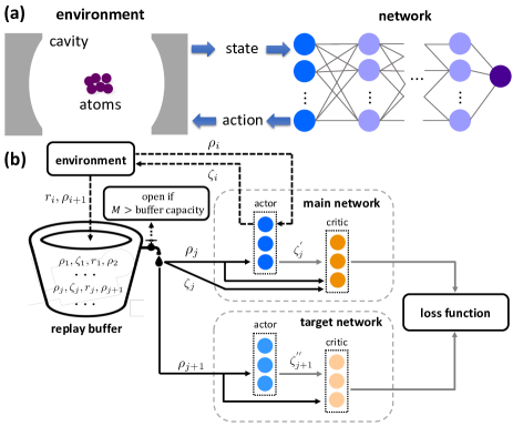
Figure 2: (a) Schematic of control generation for the enhancement of spin squeezing via reinforcement learning in a collective spin-half system coupled to a cavity. (b) Brief flow chart of the DDPG algorithm Lillicrap2015 .

In many scenarios, time-varying controls ($\zeta=\zeta(t)$) are more powerful than the constant-value controls since they provide a way larger parameter space for the control. Finding an optimal time-varying control for a given target is a major concern in quantum control. Many algorithms, including the GRAPE Khaneja2005 ; Fouquieres2011 ; Liu2017a ; Liu2017b ; Liu2020 ; Wu2019 ; Peng2018 , krotov’s method Reich2012 ; Goerz2019 , and machine learning Xu2019 ; Fosel2018 ; Bukov2018 ; An2019 ; Yang2020 ; Bukov2018 have been employed into various scenarios in quantum physics, like quantum information processing and parameter estimation, for the generation of optimal control. With respect to the spin squeezing, Pichler et al. Pichler2016 recently used the chopped random basis technique in the OAT model and obtained an enhanced behavior of squeezing than the adiabatic evolution. In the following we employ the DDPG algorithm Lillicrap2015 , an advanced reinforcement learning algorithm to study the performance of time-varying controls on the generation and storage of spin squeezing.

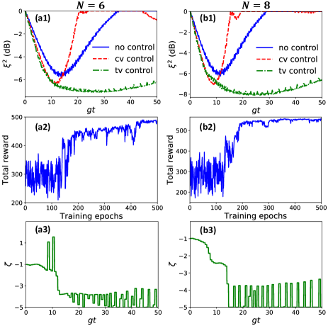
Figure 3: The results for unitary dynamics in the case of $N=6$ (a1-a3) and $N=8$ (b1-b3). Panels (a1) and (b1) show the evolution of $\xi^{2}$ (in the unit of dB) with the time-varying (tv) control (dash-dotted green lines), optimal constant-value (cv) control (dashed red lines) and without control (solid blue lines), respectively. The time-varying controls are generated via the learning with the corresponding total reward given in (a2) and (b2). Panels (a3) and (b3) give the optimal control $\zeta$ with respect to the dash-dotted green lines in (a1) and (b1).

Reinforcement learning uses a network (also called agent) to provide choices of actions for the environment to improve the reward. Its process in our case is illustrated in Fig. 2(a). The environment, consisting of the cavity and atoms, generates a dynamical quantum state according to Eq. (3), then sends it to the network, which provides an action (the control amplitude $\zeta$) accordingly. Next, the environment uses this action to evolve and generates a new state, and again sends it to the network for the generation of next control. A typical algorithm of the reinforcement learning is the Actor-Critic algorithm, in which the critic network is used to evaluate the reward that the actor obtained. The DDPG algorithm is an advanced Actor-Critic algorithm, and includes a replay buffer and additional two target networks besides the main actor and critic networks, as shown in Fig. 2(b). In the first $M$ epochs of an episode, the control amplitude is generated randomly via the main actor network and all the data of $\rho_{j}$ (density matrix), $\zeta_{j}$ (control amplitude), $r_{j}$ (reward) and $\rho_{j+1}$ are saved in the buffer (the black barrel in Fig. 2(b)). The subscript $j$ and $j+1$ represent the $j$th and $(j+1)$th time steps. The reward in our case is taken as $r_{j}=-10\mathrm{log}_{10}(\xi^{2}_{j})$ with $\xi^{2}_{j}$ the squeezing parameter at the $j$th time step. Beyond the $M$th epoch, the buffer picks a random array of data $(\rho_{j},\zeta_{j},r_{j},\rho_{j+1})$ and sends $(\rho_{j},\zeta_{j})$ to the main network and $\rho_{j+1}$ to the target network. The outputs of both networks construct the loss function, which is used to update the main networks. The target networks update much slower than the main networks since they only absorb a small weight (such as $10\%$) of the main networks.

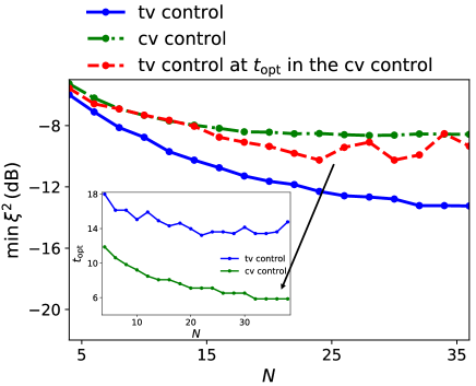
Figure 4: The variety of spin squeezing as a function of particle number $N$ for the unitary dynamics. The dash-dotted green and solid blue lines represent the minimum spin squeezing with the optimal constant-value control and time-varying control. The dashed red line represents the value of spin squeezing with the time-varying control at the time that achieve the minimum squeezing in the optimal constant-value control. The parameters are set to be the same with Fig. 3. The green and blue lines in the insert are the optimal time for the minimum squeezing in the case of optimal constant-value and time-varying controls, respectively.

The performance of the time-varying control generated via the DDPG for the noiseless case is shown in Fig. 3(a1) for $N=6$ and Fig. 3(b1) for $N=8$. The squeezing parameter $\xi^{2}$ (in the unit of dB) given by the time-varying control in both cases (dash-dotted green lines) are significantly lower than those with the optimal constant-value control (dashed red lines) and without control (solid blue lines) for almost all the time. With the time-varying control, not only the minimum value of $\xi^{2}(t)$ is lower, but $\xi^{2}(t)$ also keeps in a low position for a significant long time. The DDPG algorithm works well in our case as the total reward converges with around 500 training epochs, as shown in Figs. 3(a2) and (b2). The corresponding optimal control is illustrated in Figs. 3(a3) and (b3). Although the optimal constant-value control can provide a lower minimum value of $\xi^{2}$ than the non-controlled case, $\xi^{2}$ grows very fast afterwards, indicating a shortage on the storage of squeezing.

The behavior of spin squeezing with the increase of particle number is also a major concern in the study of this field, which is provided in Fig. 4. It shows that the advantage of time-varying control (solid blue line) on the minimum squeezing enlarges with the increase of $N$ compared to the optimal constant-value control (dash-dotted green line). The trade-off is that the corresponding evolution time is longer as given in the insert. More interestingly, the performance of time-varying control (dashed red line) at the time (green line in the insert) to achieve the minimum squeezing in the case of optimal constant-value control also goes beyond the optimal constant-value control for most values of $N$ in the plot, especially around $N=20$ to $30$, indicating that time-varying control can still present a better behavior for a short time-scale in this regime.

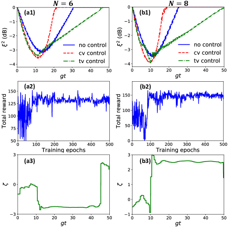
Figure 5: The results for noisy dynamics in the case of $N=6$ (a1-a3) and $N=8$ (b1-b3). Panels (a1) and (b1) show the evolution of $\xi^{2}$ (in the unit of dB) with the time-varying (tv) control (dash-dotted green lines), optimal constant-value (cv) control (dashed red lines) and without control (solid blue lines), respectively. The time-varying controls are generated via the learning with the corresponding total rewards given in (a2) and (b2). Panels (a3) and (b3) give the optimal control $\zeta(t)$ with respect to the dash-dotted green lines in (a1) and (b1). The noisy dynamics in the plots are governed by Eq. (3) with the decay rates $\kappa=\gamma=0.01g$.

Taking into account the collective noise ($\gamma=0.01g$), the advantage of time-varying control in the unitary dynamics becomes limited. The minimum value basically coincides with the one from the optimal constant-value control, as shown in Fig. 5(a1) for $N=6$ and Fig. 5(b1) for $N=8$. The corresponding total rewards and control amplitudes are given in Figs. 5(a2), (b2), (a3) and (b3), respectively. With respect to the storage of squeezing, we first define the integral

$$S=-10\int^{\infty}_{0}\log_{10}\xi^{2}(t)dt,$$ (13)

the full amount of squeezing (dB) that the system generates over all time as the quantification of the storage of squeezing. Now denote $S_{\mathrm{tv}}$, $S_{\mathrm{cv}}$, and $S_{\mathrm{no}}$ as the storage of squeezing in the noisy case with the time-varying control, optimal constant-value control (corresponds to the minimum $\min\xi^{2}$) and without control, respectively. In Fig. 5, for $N=6$, we have $S_{\mathrm{tv}}\approx 85.76$, $S_{\mathrm{cv}}\approx 46.76$, and $S_{\mathrm{no}}\approx 57.90$. These values become $S_{\mathrm{tv}}\approx 96.06$, $S_{\mathrm{cv}}\approx 43.02$, and $S_{\mathrm{no}}\approx 52.61$ for $N=8$. One can see that $S_{\mathrm{cv}}$ is less than $S_{\mathrm{no}}$ in both cases, which means under the collective noise, the performance of the optimal constant-value control on the storage of squeezing is worse than that without control. The constant-value control, including the TAT-type model, is not the optimal choice from the aspect of storage. Although the time-varying control does not present an obvious advantage on the minimum value of $\xi^{2}$, its capability of storage still significantly outperforms the other schemes, and it grows with the increase of particle number. Moreover, when the dephasing rate is larger, although the performance of time-varying control deteriorates, as shown in Fig. 6, but it is still significantly better than the non-controlled case, which shows the power of control in this model.

From the analysis above, one may notice that the constant-value controls can provide a good minimum value of $\xi^{2}$ and the time-varying controls show an advantage on the storage of squeezing. To combine the advantages of both the constant-value and time-varying controls, in the following we propose a four-step strategy to generate a new type of combined controls for the enhanced generation and storage of squeezing.

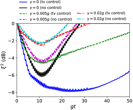
Figure 6: The evolution of $\xi^{2}$ with different dephasing rate with time-varying control or without control in the case of $N=8$. Other parameteres are set to be the same as Fig. 5.

III.3 Combined control

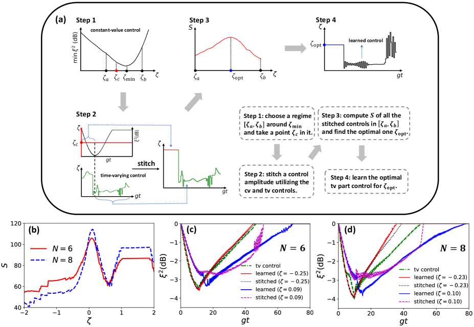
Figure 7: The illustration of the combined strategy and the corresponding results. (a) Four steps for the generation of a combined control. Step 1: choose a reasonable regime $[\zeta_{a},\zeta_{b}]$ around the optimal point $\zeta_{\min}$ that gives the minimum value of $\min\xi^{2}$ in the scenario of constant-value controls. Step 2: construct the stitched controls with the constant-value part given in $[\zeta_{a},\zeta_{b}]$. Step 3: calculate $S$ for all stitched controls and find the optimal point $\zeta_{\mathrm{opt}}$ that gives the maximum $S$. Step 4: learn the time-varying part of the $\zeta_{\mathrm{opt}}$’s stitched control and construct the final combined control. (b) $\mathcal{S}$ as a function of the stitched controls. This plot is used to search $\zeta_{\mathrm{opt}}$. (c-d) The comparison of $\xi^{2}(t)$ given by different controls for $N=6$ and $N=8$. The parameters are set the same as those in previous figures.

The proposed strategy consists of both constant-value and time-varying controls that performed at different time intervals and aims at improving the storage of squeezing. We first show how to use this strategy to generate a combined control. There are four steps to perform this strategy, as given in Fig. 7(a). The first step is to find the optimal constant-value control $\zeta_{\min}$, which corresponds to the minimum value of $\min\xi^{2}$ and then choose a reasonable regime $[\zeta_{a},\zeta_{b}]$ around $\zeta_{\min}$. Next, as the second step, we stitch a control amplitude with any value ($\zeta_{c}$) in $[\zeta_{a},\zeta_{b}]$ and the previous learned full time-varying control in this case. Specifically, denote the time that $\xi^{2}(t)$ reaches its minimum value under the constant-value control $\zeta_{c}$ as $t_{\min}$, then the stitched control in the time interval $[0,t_{\min}]$ is the constant value $\zeta_{c}$, and after $t_{\min}$, the control amplitude copies the corresponding part of the full time-varying control, as illustrated in Step 2 in Fig. 7(a). The third step is to calculate $S$ in Eq. (13) for all the stitched controls generated from all points in the regime $[\zeta_{a},\zeta_{b}]$ and find the optimal one ($\zeta_{\mathrm{opt}}$) which gives the maximum value of $S$. The last step is to replace the time-varying part of the stitched control of $\zeta_{\mathrm{opt}}$ to an optimal one that the DDPG algorithm finds. This is the final combined control.

In this strategy, the reward is still taken as the squeezing parameter, i.e., $r_{j}=-10\mathrm{log}_{10}(\xi^{2}_{j})$. In the DDPG algorithm, the actual target for the agent to maximize at $j$th time step is the discount reward $R_{j}=\sum^{k}_{j^{\prime}=j}\mu^{j^{\prime}-j}r_{j^{\prime}}$ with $\mu\in(0,1]$ the discount factor and $k$ the number of time steps. The design of discount reward is to reflect the variety of influence for the control at $j$th time step on the rewards afterwards, which reduces with the increase of time intervals. As the discount reward contains the information of rewards for all time afterwards, it basically has a positive correlation with $S$ defined in Eq. (13). Hence, we can still use this reward form for the optimization of the storage of squeezing.

In many realistic cases, finding all the learned time-varying parts in the entire regime $[\zeta_{a},\zeta_{b}]$ for the calculation of $S$ could be very time-consuming, this is the reason why we need to construct the stitched controls in the second step. The stitched control only requires an episode (500 epochs in our case) of Learning to find an optimal full time-varying control. Different constant-value parts may have different time [$t_{\min}(\zeta)$] to reach the minimum value of $\min\xi^{2}$, hence, one may need to truncate different parts of the full time-varying control for the further construction of the stitched controls.

Utilizing this strategy, the behaviors of $\mathcal{S}$ in our model are shown in Fig. 7(b) for both $N=6$ (solid red line) and $N=8$ (dashed blue line). The maximum values of $S$ are saturated by very small values of $\zeta$, namely, $\zeta_{\mathrm{opt}}\approx 0.09$ for $N=6$ and $0.10$ for $N=8$. The performances of both stitched and combined (learned) controls that final obtained are given in Figs. 7(c), and 7(d) for $N=6$ and $N=8$, respectively. In the case of $N=6$, the performances of the stitched control (dotted black line) and learned control (solid red line) with the $\zeta_{\min}$ point ($\zeta=-0.25$) as the constant-value parts basically coincide with each other, and also coincide with the performance given by the full time-varying control (dash-dotted green line). Hence, one does not need a full time-varying control here for the generation and storage of squeezing, the stitched or the learned control can realize the same performance but with a more simple and stable control amplitude due to the fact that both these controls have a constant-value part. In the case of $N=8$, the stitched and learned controls with the $\zeta_{\min}$ point ($\zeta=-0.23$) also coincide with each other, however, different with the case of $N=6$, they are worse than that given by the full time-varying control, which indicates that it is not a good choice to use $\xi_{\min}$ for the construction of the combined control.

Varying from the phenomenon with the $\zeta_{\min}$ points, the stitched and final combined controls with $\zeta_{\mathrm{opt}}$ as the constant-value part show very different behaviors, which supports our strategy that $\zeta_{\mathrm{opt}}$, rather than $\zeta_{\min}$, should be used for the construction of final combined controls. The squeezing parameters with the stitched controls (dashed purple lines in Figs. 7(c-d)) have a bad minimum value compared to the full time-varying controls and grows very fast after the time around $gt=50$, which may be due to the fact the time-varying part of this control comes from the full time-varying control, and this part becomes dominant with the passage of time. However, the final (learned) combined controls show a very good performance. As a matter of fact, the existence of squeezing with the combined controls lasts much longer than those with other controls. The squeezing parameters for the combined controls (solid blue lines in Figs. 7(c-d)) vanish at around $gt=70$ for $N=6$ and $gt=80$ for $N=8$. In the meantime, the full time-varying controls can only provide a lifetime of squeezing within or around $gt=50$ in both cases. Moreover, the storage of squeezing with the combined controls also outperforms that with the time-varying controls. Quantitatively to say, $S_{\mathrm{c}}$ ($S$ for the combined controls) is about $117.60$ for $N=6$ and $129.76$ for $N=8$, which increases about $35\%\sim 40\%$ compared to $S_{\mathrm{tv}}$. Besides, the minimum values of $\xi^{2}(t)$ are very close to those with the time-varying controls in both cases.

In physics, an intuitive picture for the storage of squeezing with control is to freeze the squeezing dynamics after $\xi^{2}$ reaches its minimum Wu2015 . Indeed, from the aspect of optimal squeezing angle $\varphi_{\mathrm{opt}}$ shown in Fig. 8, the learned time-varying control in the unitary dynamics does try to keep $\varphi_{\mathrm{opt}}$ (dash-dotted green line) around the angle to reach the minimum squeezing (dotted black line), however, when the noise exists, it is difficult for the control to prevent $\varphi_{\mathrm{opt}}$ (dashed blue line) deviating from the angle for $\min\xi^{2}$ (dotted purple line), and the combined control can slow down this deviation of $\varphi_{\mathrm{opt}}$ (solid red line) and thus enlarge the lifetime of squeezing.

All the facts above indicate that the combined controls obtained via our strategy present a very good performance on both the generation and storage of squeezing. It is not only more stable and simpler than a full time-varying control, but can also balance the trade-off between the minimum values of $\xi^{2}(t)$ and the full amount of the generated squeezing. Therefore, this strategy could be very helpful in the realistic experiments for the generation of spin squeezing.

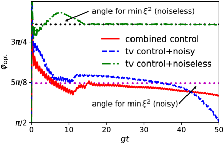
Figure 8: The evolution of optimal squeezing angle in the case of the time-varying control under noiseless dyanmics (dash-dotted green line) and noisy dynamics (dashed blue line), and in the case of the combined control (solid red line). The dotted pruple and black lines represent the angles for $\min\xi^{2}$ under noisy and noiseless dynamics. The decay rates for the blue and red lines are set to be $\kappa=\gamma=0.01g$. Other parameters are set to be same with the previous figures.

IV conclusion and outlook

In conclusion, we have studied the generation and storage of spin squeezing in the collective spin system coupled to a bosonic field. Three control strategies, constant-value, time-varying, and combined controls are considered. With a proper constant-value control, this system can simulate the one- and two-axis twisting models. The time-varying controls show very good performances under the unitary dynamics, however, when the collective noise is involved, this advantage becomes not significant.

To deal with this situation, we further propose a strategy for the construction of combined controls. This strategy contains four steps. The first step is finding an optimal constant-value control $\zeta$ ($\zeta_{\min}$) that gives the lowest value of $\min\xi^{2}$, and choose a reasonable regime $[\zeta_{a},\zeta_{b}]$ around it. The second step is constructing a stitched control with the constant-value part chosen in $[\zeta_{a},\zeta_{b}]$ and the time-varying part copied from the full time-varying control. The third step is calculating $S$ for all the stitched controls and finding the optimal value $\zeta_{\mathrm{opt}}$ which gives the maximum value of $S$. The fourth step is replacing the time-vary part of the stitched control of $\zeta_{\mathrm{opt}}$ by the one obtained via the learning algorithms, which is just the final combined control. This combined control is more simple and stable than a full time-varying control. It not only gives a comparable minimum value of $\xi^{2}$ with respect to the full time-varying control, but also provides a better lifetime and larger full amount of squeezing (quantified by $S$). Hence, this combined strategy is very promising to be applied in practical experiments for a better generation and storage of spin squeezing.

It is known that the performance of learning might be not good when the action (control) space is large. Hence, a restriction on the waveform of control field could reduce the action space and help to find an optimal solution in this space, however, it may also limit the performance of control since the global optimal control may not be in this chosen subspace. In the meantime, the computational complexities for the dynamics could dramatically increase when the scale of the system grows. Therefore, how to make the learning algorithms efficient for a free waveform and how to apply it into large-scale systems for the sake of enhanced spin squeezing still remains a challenge in this field. More techniques like the matrix product states may be needed to be involved, and the learning algorithms may also need to be adjusted correspondingly.

*

Appendix A Simulation of one- and two-axis twisting models with constant-value controls

Here we provide the thorough calculation on the simulation of one-axis twisting and two-axis twisting type model. Recall the original Hamiltonian is

$$H_{0}=\omega_{c}a^{\dagger}a+\omega_{z}J_{z}+gJ_{x}(a^{\dagger}+a),$$ (14)

and the control Hamiltonian is

$$H_{\mathrm{c}}(t)=\zeta\nu\cos(\nu t)J_{z},$$ (15)

where $\zeta$ is a time-independent constant. Notice that the transformation

$$V(t) := \mathcal{T}\exp\left[i\int_{0}^{t}(H_{0}+H_{\mathrm{c}})d\tau\right]$$ (16)

$$= \exp\left\{i\omega_{c}ta^{\dagger}a+i\left[\omega_{z}t+\zeta\sin(\nu t)\right]J_{z}\right\}$$

with $\mathcal{T}$ the time-ordering operator, then in the rotating frame defined by $V(t)$, the transformed Hamiltonian becomes

$$\tilde{H}(t)$$

$$= V(t)H(t)V^{\dagger}(t)-iV(t)\partial_{t}{V}^{\dagger}(t)$$

$$= g\left\{\cos\left[\omega_{z}t+\zeta\sin(\nu t)\right]J_{x}-\sin\left[\omega_{z}t+\zeta\sin(\nu t)\right]J_{y}\right\}$$

$$\times(a^{\dagger}e^{i\omega_{c}t}+ae^{-i\omega_{c}t})$$

$$= \frac{g}{2}\left\{e^{i[\omega_{z}t+\zeta\sin(\nu t)]}J_{+}+e^{-i[\omega_{z}t+\zeta\sin(\nu t)]}J_{-}\right\}$$

$$\times(a^{\dagger}e^{i\omega_{c}t}+ae^{-i\omega_{c}t})$$

$$= g\mathrm{Re}\!\left(\!e^{i(\omega_{c}+\omega_{z})t}e^{i\zeta\sin(\nu t)}J_{+}a^{\dagger}\!+\!e^{-i(\omega_{c}-\omega_{z})t}e^{i\zeta\sin(\nu t)}J_{+}a\right)\!,$$

where $\mathrm{Re}(\cdot)$ is the real part. Utilizing the Jacobi–Anger expansion

$$e^{i\zeta\sin(\nu t)}=\sum^{\infty}_{n=-\infty}\mathcal{J}_{n}(\zeta)e^{in\nu t}$$ (17)

with $\mathcal{J}_{n}(\zeta)$ the $n$th Bessel function of the first kind, $\tilde{H}$ can be further rewritten into

$$\tilde{H} = \frac{g}{2}\sum_{m=-\infty}^{\infty}\mathcal{J}_{m}(\zeta)e^{i\Delta_{m}t}J_{+}a^{\dagger}$$

$$+\frac{g}{2}\sum_{n=-\infty}^{\infty}\mathcal{J}_{n}(\zeta)e^{i\left(n\nu-\delta\right)t}J_{+}a+\mathrm{H.c.},$$

where $\Delta_{m}=m\nu+\omega_{c}+\omega_{z}$, $\delta=\omega_{c}-\omega_{z}$, and H.c. represents the Hermitian conjugate. Under the condition $\nu\gg g,\delta$, $\tilde{H}$ approximates to

$$\tilde{H}\approx(g_{0}J_{+}ae^{-i\delta t}+g_{m_{0}}J_{-}ae^{-i\Delta_{m_{0}}t})+\mathrm{H.c.}$$ (18)

with $g_{0}=g\mathcal{J}_{0}(\zeta)/2$ and $g_{m_{0}}=g\mathcal{J}_{m_{0}}(\zeta)/2$. Here $m_{0}$ is an optimal integer that make $|m\nu+\omega_{\mathrm{c}}+\omega_{z}|$ minimum. A similar approach Huang2017 has been applied in quantum Rabi model to manipulate the counter-rotating interactions. Now take the condition $\delta=\Delta_{m_{0}}\equiv\Delta$, that is $m_{0}=-2[\omega_{z}/\nu]$ ($[\cdot]$ is the rounding function), and transform $\tilde{H}$ back to a non-rotating frame with $V_{1}=e^{i\Delta a^{\dagger}at}$, namely, $\tilde{H}=V_{1}H_{1}V_{1}^{\dagger}-iV_{1}\partial_{t}V_{1}^{\dagger}$, then

$$H_{1} = \Delta a^{\dagger}a+\frac{g}{2}\left[J_{0}(\zeta)J_{+}+J_{m_{0}}(\zeta)J_{-}\right]a+\mathrm{H.c.}$$ (19)

$$= \Delta a^{\dagger}a+g(\Sigma^{\dagger}a+\Sigma a^{\dagger})$$

with $\Sigma=[\mathcal{J}_{0}(\zeta)J_{-}+\mathcal{J}_{m_{0}}(\zeta)J_{+}]/2$.

Figure 9: The dynamics of the fidelity between the evolved states given by the original Hamiltonian in Eqs. (14) and (15) and the effective Hamiltonian in Eq. (24).

In the regime of large detunings $\Delta\gg g>g_{0},g_{m_{0}}$, $\tilde{H}$ can be approximately diagonalized by the transformation $e^{R}H_{1}e^{-R}=H_{\mathrm{eff}}$ with

$$R=\frac{g}{\Delta}(\Sigma a^{\dagger}-\Sigma^{\dagger}a).$$ (20)

Truncating to the second order of $g/\Delta$, and notice the fact that

$$[R,H_{1}] = -g\Sigma a^{\dagger}-g\Sigma^{\dagger}a-\frac{g^{2}}{\Delta}(\Sigma\Sigma^{\dagger}+\Sigma^{\dagger}\Sigma)$$ (21)

$$+\frac{g^{2}}{\Delta}[\Sigma,\Sigma^{\dagger}]aa^{\dagger}+\frac{g^{2}}{\Delta}[\Sigma,\Sigma^{\dagger}]a^{\dagger}a,$$

and

$$[R,[R,H_{1}]] = \frac{g^{2}}{\Delta}\left(\Sigma\Sigma^{\dagger}+\Sigma^{\dagger}\Sigma\right)-\frac{g^{2}}{\Delta}[\Sigma,\Sigma^{\dagger}]\left(2a^{\dagger}a+1\right)$$ (22)

$$= -\frac{2g^{2}}{\Delta}\left([\Sigma,\Sigma^{\dagger}]a^{\dagger}a-\Sigma^{\dagger}\Sigma\right),$$

$H_{\mathrm{{eff}}}$ then reduces to

$$H_{\mathrm{{eff}}} = H_{1}+[R,H_{1}]+\frac{1}{2}[R,[R,H_{1}]]+\cdots$$ (23)

$$= \Delta a^{\dagger}a+\frac{g^{2}}{\Delta}[\Sigma,\Sigma^{\dagger}]a^{\dagger}a-\frac{g^{2}}{\Delta}\Sigma^{\dagger}\Sigma.$$

Substituting the expression of $\Sigma$ into the equation above, one can have

$$H_{\mathrm{{eff}}} = \Delta a^{\dagger}a-\left(\frac{g_{0}^{2}-g_{m_{0}}^{2}}{\Delta}\right)(1+2a^{\dagger}a)J_{z}$$ (24)

$$+\frac{\left(g_{0}-g_{m_{0}}\right)^{2}}{\Delta}J_{z}^{2}-\frac{4g_{0}g_{m_{0}}}{\Delta}J_{x}^{2},$$

in which the constant term has been neglected. Utilizing this Hamiltonian, an effective one-axis twisting Hamiltonian can be realized by taking $g_{0}=g_{m_{0}}$, i.e., $\mathcal{J}_{0}(\zeta)=\mathcal{J}_{m_{0}}(\zeta)$. Under this condition, $H_{\mathrm{eff}}$ reduces to $-\chi J_{x}^{2}$, with $\chi=\frac{g^{2}}{\Delta}\mathcal{J}_{m_{0}}^{2}(\zeta)$. In the mean time, the two-axis twisting type Hamiltonian can be obtained by taking $(g_{0}-g_{m_{0}})^{2}=4g_{0}g_{m_{0}}$, which is equivalent to $\mathcal{J}_{0}(\zeta)=\left(3\pm 2\sqrt{2}\right)\mathcal{J}_{m_{0}}(\zeta)$. This condition let $H_{\mathrm{eff}}$ reduce to $-\lambda(J_{x}^{2}-J_{z}^{2})+\lambda^{\prime}(1+2a^{\dagger}a)J_{z}$, where $\lambda=\frac{4g_{0}g_{m_{0}}}{\Delta}=\frac{g^{2}(3\pm 2\sqrt{2})}{\Delta}\mathcal{J}_{m_{0}}^{2}(\zeta)$ and $\lambda^{\prime}=-\frac{g_{0}^{2}-g_{m_{0}}^{2}}{\Delta}$. The second term in the equation above can be (on average) eliminated through a dynamical decoupling protocol, which makes $H_{\mathrm{eff}}$ a traditional two-axis twisting Hamiltonian $-\lambda(J_{x}^{2}-J_{z}^{2})$.

To show the validity of this effective Hamiltonian, the fidelity between the evolved states given by the original Hamiltonians (Eqs. (14) and (15)) and the effective Hamiltonian above are shown in Fig. 9 for the unitary dynamics with $N=6$. Other parameters are set as $\omega_{z}=110$, $\omega_{c}=100$, $\nu=200$, $g=1$, and $\zeta=2.569$ (TAT-type). The evolution of fidelity shows that the effective Hamiltonian works well ($>0.999$) within the time point $gt=50$.

References

- (1) H. P. Yuen, Two-photon coherent states of the radiation field, Phys. Rev. A 13, 2226 (1976).
- (2) D. F. Walls, G.J. Milburn, Quantum Optics (Springer-Verlag, 1994).
- (3) M. O. Scully, M.S. Zubairy, Quantum Optics (Cambridge University press, 1997).
- (4) C. M. Caves, Quantum-mechanical noise in an interferometer, Phys. Rev. D 23, 1693 (1981).
- (5) M. D. Lang and C. M. Caves, Optimal Quantum-Enhanced Interferometry Using a Laser Power Source, Phys. Rev. Lett. 111, 173601 (2013).
- (6) H. Grote, K. Danzmann, K. L. Dooley, R. Schnabel, J. Slutsky, and H. Vahlbruch, First Long-Term Application of Squeezed States of Light in a Gravitational-Wave Observatory, Phys. Rev. Lett. 110, 181101 (2013).
- (7) J. Ma, X. Wang, C. P. Sun, and F. Nori, Quantum spin squeezing, Phys. Rep. 509, 89 (2011).
- (8) L. Pezzè, A. Smerzi, M. K. Oberthaler, R. Schmied, and P. Treutlein, Quantum metrology with nonclassical states of atomic ensembles, Rev. Mod. Phys. 90, 035005 (2018).
- (9) M. Kitagawa, M. Ueda, Squeezed spin states, Phys. Rev. A 47, 5138 (1993).
- (10) D. J. Wineland, J. J. Bollinger, W. M. Itano, F. L. Moore, D. J. Heinzen, Spin squeezing and reduced quantum noise in spectroscopy, Phys. Rev. A 46, 6797(R) (1992).
- (11) D. J. Wineland, J. J. Bollinger, W. M. Itano, and D. J. Heinzen, Squeezed atomic states and projection noise in spectroscopy, Phys. Rev. A 50, 67 (1994).
- (12) A. D. Cronin, J. Schmiedmayer, and D. E. Pritchard, Optics and interferometry with atoms and molecules, Rev. Mod. Phys. 81, 1051 (2009).
- (13) J. D. Sau, S. R. Leslie, M. L. Cohen, and D. M. Stamper-Kurn, Spin squeezing of high-spin, spatially extended quantum fields, New J. Phys. 12, 085011 (2010).
- (14) G. Vitagliano, P. Hyllus, I. L. Egusquiza, and G. Tóth, Spin Squeezing Inequalities for Arbitrary Spin, Phys. Rev. Lett. 107, 240502 (2011).
- (15) O. Gühne, G. Tóth, Entanglement detection, Phys. Rep. 474, 1 (2009).
- (16) G. R. Jin, Y. C. Liu and W. M. Liu, Spin squeezing in a generalized one-axis twisting model, New J. Phys. 11, 073049 (2009).
- (17) G. R. Jin and S. W. Kim, Storage of Spin Squeezing in a Two-Component Bose-Einstein Condensate, Phys. Rev. Lett. 99, 170405 (2007).
- (18) S. D. Bennett, N. Y. Yao, J. Otterbach, P. Zoller, P. Rabl, and M. D. Lukin, Phonon-Induced Spin-Spin Interactions in Diamond Nanostructures: Application to Spin Squeezing, Phys. Rev. Lett. 110, 156402 (2013).
- (19) W. Zhong, J. Liu, J. Ma and X. G. Wang, Quantum Fisher information and spin squeezing in one-axis twisting model, Chin. Phys. B 23, 060302 (2014).
- (20) C. Gross, T. Zibold, E. Nicklas, J. Estève, and M. K. Oberthaler, Nonlinear atom interferometer surpasses classical precision limit, Nature 464, 1165–1169 (2010).
- (21) M. F. Riedel, P. Böhi, Y. Li, T. W. Hänsch, A. Sinatra, and P. Treutlein, Atom-chip-based generation of entanglement for quantum metrology, Nature 464, 1170–1173 (2010).
- (22) K. Helmerson and L. You, Creating Massive Entanglement of Bose-Einstein Condensed Atoms, Phys. Rev. Lett. 87, 170402 (2001).
- (23) M. Zhang, Kristian Helmerson, and L. You, Entanglement and spin squeezing of Bose-Einstein-condensed atoms, Phys. Rev. A 68, 043622 (2003).
- (24) H. T. Ng, C. Law, and P. Leung, Quantum-correlated double-well tunneling of two-component Bose-Einstein condensates, Phys. Rev. A 68, 013604 (2003).
- (25) Y. C. Liu, Z. F. Xu, G. R. Jin, and L. You, Spin Squeezing: Transforming One-Axis Twisting into Two-Axis Twisting, Phys. Rev. Lett. 107, 013601 (2011).
- (26) Y. C. Zhang, X. F. Zhou, X. Zhou, G. C. Guo, and Z. W. Zhou, Cavity-Assisted Single-Mode and Two-Mode Spin-Squeezed States via Phase-Locked Atom-Photon Coupling, Phys. Rev. Lett. 118, 083604 (2017).
- (27) P. Groszkowski, H.-K. Lau, C. Leroux, L. C. G. Govia, A. A. Clerk, Heisenberg-limited spin-squeezing via bosonic parametric driving, Phys. Rev. Lett. 125, 203601 (2021).
- (28) L. K. Thomsen, S. Mancini, and H. M. Wiseman, Continuous quantum nondemolition feedback and unconditional atomic spin squeezing, J. Phys. B 35, 4937 (2002).
- (29) W. Qin, Y.-H. Chen, X. Wang, A. Miranowicz and F. Nori, Strong spin squeezing induced by weak squeezing of light inside a cavity, Nanophotonic 9, 4853–4868 (2020).
- (30) T. P. Lillicrap, J. J. Hunt, A. Pritzel, N. Heess, T. Erez, Y. Tassa, D. Silver, and D. Wierstra, Continuous control with deep reinforcement learning, arXiv:1509.02971.
- (31) M. Mohri, A. Rostamizadeh, and A. Talwalkar, Foundations of Machine Learning (The MIT press, 2018).
- (32) R. Hafner and M. Riedmiller, Reinforcement learning in feedback control: Challenges and benchmarks from technical process control, Mach. Learn. 84, 137-169 (2011).
- (33) S. Kevine, A. Kumar, G. Tucker, and J. Fu, Offline reinforcement learning: tutorial, review, and perspectives on open problems, arXiv: 2005.01643.
- (34) G. Carleo, I. Cirac, K. Cranmer, L. Daudet, M. Schuld, N. Tishby, L. Vogt-Maranto, and L. Zdeborová, Machine learning and the physical sciences, Rev. Mod. Phys. 91, 045002 (2019).
- (35) M. Krenn, M. Erhard, and A. Zeilinger, Computer-inspired quantum experiments, Nat. Rev. Phys. 2, 649–661 (2020).
- (36) E. P. L. van Nieuwenburg, Y. H. Liu and S. D. Huber, Learning phase transitions by confusion, Nat. Phys. 13, 435-439 (2017).
- (37) Y. H. Liu and E. P. L. van Nieuwenburg, Discriminative Cooperative Networks for Detecting Phase Transitions, Phys. Rev. Lett. 120, 176401 (2018).
- (38) Y. Che, C. Gneiting, T. Liu and F. Nori, Topological quantum phase transitions retrieved through unsupervised machine learning, Phys. Rev. B 102, 134213 (2020).
- (39) H. Xu, J. Li, L. Liu, Y. Wang, H. Yuan and X. Wang, Generalizable control for quantum parameter estimation through reinforcement learning, npj Quantum Inf. 5, 82 (2019).
- (40) A. Hentschel and B. C. Sanders, Machine Learning for Precise Quantum Measurement, Phys. Rev. Lett. 104, 063603 (2010).
- (41) A. Hentschel and B. C. Sanders, Efficient Algorithm for Optimizing Adaptive Quantum Metrology Processes, Phys. Rev. Lett. 107, 233601 (2011).
- (42) X. M. Zhang, Z. W. Cui, X. Wang, and M. H. Yuan, Automatic spin-chain learning to explore the quantum speed limit, Phys. Rev. A 97, 052333 (2018).
- (43) J. Wang, S. Paesani, R. Santagati, S. Knauer, A. A. Gentile, N. Wiebe, M. Petruzzella, J. L. O’Brien, J. G. Rarity, A. Laing, and M. G. Thompson, Experimental quantum Hamiltonian learning, Nat. Phys. 13, 551–555 (2017).
- (44) M. Krenn, M. Malik, R. Fickler, R. Lapkiewicz, and A. Zeilinger, Automated Search for new Quantum Experiments, Phys. Rev. Lett. 116, 090405 (2016).
- (45) A. A. Melnikov, H. P. Nautrup, M. Krenn, V. Dunjko, M. Tiersch, A. Zeilinger, and H. J. Briegel, Active learning machine learns to create new quantum experiments, Proc. Natl. Acad. Sci. USA 115, 1221–1226 (2018).
- (46) F. Chen, J.-J. Chen, L.-N. Wu, Y.-C. Liu, and L. You, Extreme spin squeezing from deep reinforcement learning, Phys. Rev. A 100, 041801(R) (2019).
- (47) D. A. Steck, Rubidium 87D Line Data, available online at https://steck.us/alkalidata (revision 2.2.1, 21 November 2019).
- (48) N. Khaneja, T. Reiss, C. Hehlet, T. Schulte-Herbruggen, and S. J. Glaser, Optimal control of coupled spin dynamics: Design of NRM pulse sequences by gradient ascent algorithms, J. Magn. Reson. 172, 296-305 (2005).
- (49) P. de Fouquieres, S. G. Schirmer, S. J. Glaser, I. Kuprov, Second order gradient ascent pulse engineering, J. Magn. Reson. 212, 412-417 (2011).
- (50) J. Liu and H. Yuan, Quantum parameter estimation with optimal control, Phys. Rev. A 96, 012117 (2017).
- (51) J. Liu and H. Yuan, Control-enhanced multiparameter quantum estimation, Phys. Rev. A 96, 042114 (2017).
- (52) J. Liu, H. Yuan, X.-M. Lu, and X. Wang, Quantum Fisher information matrix and multiparameter estimation, J. Phys. A: Math. Theor. 53, 023001 (2020).
- (53) R.-B. Wu, H. Ding, D. Dong, and X. Wang, Learning robust and high-precision quantum controls, Phys. Rev. A 99, 042327 (2019).
- (54) M. Jiang, J. Bian, X. Liu, H. Wang, Y. Ji, B. Zhang, X. Peng, and J. Du, Numerical optimal control of spin systems at zero magnetic field, Phys. Rev. A 97, 062118 (2018).
- (55) D. Reich, M. Ndong, and C. P. Koch, Monotonically convergent optimization in quantum control using Krotov’s method, J. Chem. Phys. 136, 104103 (2012).
- (56) M. H. Goerz, D. Basilewitsch, F. Gago-Encinas, M. G. Krauss, K. P. Horn, D. M. Reich, and C. P. Koch, Krotov: A Python implementation of Krotov’s method for quantum optimal control, Sci. Post Phys. 7, 080 (2019).
- (57) T. Fosel, P. Tighineanu, T. Weiss, and F. Marquardt, Reinforcement Learning with Neural Networks for Quantum Feedback, Phys. Rev. X 8, 031084 (2018).
- (58) Z. An and D. Zhou, Deep reinforcement learning for quantum gate control, EPL 126, 60002 (2019).
- (59) X. Yang, X. Chen, J. Li, X. Peng, and R. Laflamme, Hybrid quantum-classical approach to enhanced quantum metrology, Sci. Rep. 11, 672 (2021).
- (60) M. Bukov, A. G. R. Day, D. Sels, P. Weinberg, A. Polkovnikov, and P. Mehta, Reinforcement Learning in Different Phases of Quantum Control, Phys. Rev. X 8, 031086 (2018).
- (61) T. Pichler, T. Caneva, S. Montangero, M. D. Lukin, and T. Calarco, Noise-resistant optimal spin squeezing via quantum control, Phys. Rev. A 93, 013851 (2016).
- (62) L.-N. Wu, M. K. Tey, and L. You, Persistent atomic spin squeezing at the Heisenberg limit, Phys. Rev. A 92, 063610 (2015).
- (63) J. F. Huang, J. Q. Liao, L. Tian, and L. M. Kuang, Manipulating counter-rotating interactions in the quantum Rabi model via modulation of the transition frequency of the two-level system, Phys. Rev. A 96, 043849 (2017).