A coupled electromagnetic-thermomechanical approach for the modeling of electric motors

Abstract

Future developments of lighter, more compact and powerful motors – driven by environmental and sustainability considerations in the transportation industry – involve higher stresses, currents and electromagnetic fields. Strong couplings between mechanical, thermal and electromagnetic effects will consequently arise and a consistent multiphysics modeling approach is required for the motors’ design. Typical simulations – the bulk of which are presented in the electrical engineering literature – involve a stepwise process, where the resolution of Maxwell’s equations provides the Lorentz and magnetic forces which are subsequently used as the external body forces for the resolution of Newton’s equations of motion.

The work presented here proposes a multiphysics setting for the boundary value problem of electric motors. Using the direct approach of continuum mechanics, a general framework that couples the electromagnetic, thermal and mechanical fields is derived using the basic principles of thermodynamics. Particular attention is paid to the derivation of the coupled constitutive equations for isotropic materials under small strain but arbitrary magnetization. As a first application, the theory is employed for the analytical modeling of an idealized asynchronous motor for which we calculate the electric current, magnetic, stress and temperature fields as a function of the applied current and slip parameter. The different components of the stress tensor and body force vector are compared to their purely mechanical counterparts due to inertia, quantifying the significant influence of electromagnetic phenomena.

1 Introduction

The increasing importance and market share of hybrid and purely electric vehicles, in the quest to reduce their carbon footprint, urges the electric motor industry to develop higher performance products with reduced manufacturing costs. New goals are set by various government agencies and industrial associations (López et al., 2019) in terms of efficiency, reliability, power losses, power density, higher rotation velocity and reduced weight. Novel electric motor designs are needed to overcome these technological challenges in order to comply with the aforementioned technical objectives and appropriate modeling tools must be developed.

Modeling of electric motors has in the past been a topic studied predominantly by the electrical engineering community. The focus has been on the calculation of the magnetic field and resulting torque and iron losses for different motor designs using both analytical, (e.g. see: Boules (1984); Zhu et al. (1993); Lubin et al. (2011)) and numerical (e.g. see: Chari and Silvester (1971); Silvester et al. (1973); Abdel-Razek et al. (1982); Arkkio (1987); Huppunen et al. (2004)) methods. A particular class of analytical methods, termed “subdomain methods” (e.g. see: Devillers et al. (2016)) constitute an approximate but efficient tool for evaluating the magnetic characteristics of motor concepts at the preliminary design stage.

In the late 90s, stress calculations in electric motors have appeared as a result of noise and vibrations concerns. As pointed out by Reyne et al. (1987), the first difficulty encountered was the evaluation of the electromagnetic body forces, for which various authors gave different expressions, due to the absence of a consistent continuum electrodynamics framework. The multiplicity of the different formulations, direct as well as variational, for the thermomechanical-electromagnetic continuum, is a source of confusion. Different (albeit equivalent) expressions for the Maxwell stress and electromagnetic body forces can be obtained and are thus responsible for the difficulty in the correct modeling of stresses in electric motors. For further discussion on this issue, the interested reader is referred to the article by Kankanala and Triantafyllidis (2004) and book by Hutter et al. (2007). The first FEM computations for stresses in electric motors used a stepwise, uncoupled, approach: electric currents and magnetic fields where calculated using a purely electromagnetic model; the electromagnetic body force vector was then introduced as the external body force in a purely mechanical model to calculate the resulting stress state (e.g. see: Reyne et al. (1988); Javadi et al. (1995)).

The above-described approximate methods are inadequate to deal with the true multiphysics nature of the electric motor problem. The magnetic fields and currents generate the body forces driving the motor. These become even more important in the ferrous materials with high magnetic susceptibility that are used to enhance and channel the magnetic flux for improved motor performance. Moreover, these materials have intrinsic strongly coupled magnetic and mechanical behavior, with the material magnetization influencing the stress state via the “magnetostriction” phenomenon and the stress state of the material also impacting its magnetization via “inverse magnetostriction (Daniel et al., 2020). Moreover, strong currents influence temperature due to ohmic effects and so on. Recognizing these issues, recent work by Fonteyn et al. (2010, 2010a, 2010b) takes into account magnetoelastic coupling effects for the numerical stress calculation in electric motors. However several approximations are used (e.g. a small strain approximation involving non frame-indifferent invariants and the angular momentum balance principle is not imposed), thermal fields are not considered and resulting stresses are not compared to inertial terms, motivating the present study.

The goal of this work is a thermodynamically consistent formulation that couples the electromagnetic, thermal and mechanical effects for the boundary value problem of electric motors. On the theoretical side, general continuum mechanics theories coupling thermomechanical and electromagnetic effects in solids started back in the 1950s and 1960s. Although a literature review is beyond the scope of this study, a few comments are helpful to put in perspective the present work. As in Fonteyn et al. (2010a, b), the modeling approach followed here is the “direct” method which uses conservation laws of continuum mechanics and the thermodynamics procedure introduced by Coleman and Noll (1963) to obtain the problem’s governing equations and constitutive laws; a very readable account is presented in the book by Kovetz (2000). For the electric motor applications of interest the “eddy current” simplification of the problem is adopted (see Hiptmair and Ostrowski (2005) for a justification in linear materials) that neglects electric polarization and displacement currents for low frequency electric fields. This theory is subsequently used to obtain the analytical solution of an idealized asynchronous motor for which we calculate the electric current, magnetic, stress and temperature fields. The stress tensor and body force vector are compared to their purely mechanical counterparts due to inertia, quantifying the significant influence of electromagnetic phenomena, a novelty in this area to the best of the author’s knowledge.

The presentation is organized as follows: following this introduction in Section 1, the general formulation for the boundary value problem for electric motors is given in Section 2, where particular attention is paid to the derivation of the coupled constitutive equations for isotropic materials under small strain but arbitrary magnetization. The analytical model of an idealized asynchronous motor is presented in Section 3, where we calculate the magnetic field for the rotor and airgap in addition to the temperature field, the magnetic, total and elastic stresses in the rotor and the torque as a function of the applied current and the slip parameter (equivalent to the mechanical torque). The results for three different rotor materials (electric steel, copper and aluminum) using realistic geometric and operational regime values and material parameters are presented in Section 4 and the work is concluded with a critical review and suggestions for future work in Section 5. The detailed derivations of the constitutive laws for isotropic materials under small strain but arbitrary magnetization are given in A, detailed expressions for some elastic stress solution components are given in B while the determination of the magnetostrictive coefficient is presented in C.

2 Boundary value problem for electric motors

The general formulation of the coupled electromagnetic-thermomechanical boundary value problem for electric motors is presented in this section. Coordinate-free (dyadic) continuum mechanics notation is used with bold scripts referring to tensors, regular scripts to scalars. Eulerian fields are written using lowercase letters, while capital letters are used for their Lagrangian counterparts. A superposed dot $\overset{\boldsymbol{.}}{f}$ denotes the total time derivative of field $f$. The method adopted is the current configuration, direct approach of continuum mechanics and tacitly assumes adequate smoothness of the fields involved. Unless stated otherwise, all field quantities are functions of the current position $\boldsymbol{x}$ and time $t$. Although the governing equations for electromagnetic continua are known (see Kovetz (2000)), for self-sufficiency and clarity of the work a brief presentation is given in this section.

2.1 General governing equations

The general equations of the problem can be distinguished in three groups, as presented in the subsections below: electromagnetics (Gauss and Ampère), mechanics (conservation of mass, balance of linear and angular momenta) and thermodynamics (conservation of energy and entropy inequality). In the applications considered the interfaces encountered are not moving with respect to matter, since they are either a free surface boundary or an interface between two different materials and hence in the sequel the interface velocity is the material velocity at the interface: $\boldsymbol{v}_{s}=\overset{\boldsymbol{.}}{\boldsymbol{x}}$.

2.1.1 Electromagnetics

Maxwell-Gauss law relates the electric displacement $\boldsymbol{d}$ to the free electric charge density $q$. The differential equation and the associated interface condition (in the absence of surface charges) are

$${\scriptstyle\boldsymbol{\nabla}}\!\boldsymbol{\cdot}\!\boldsymbol{d}=q\;;\quad\boldsymbol{n}\!\boldsymbol{\cdot}\!\llbracket\boldsymbol{d}\rrbracket=0\;,$$ (2.1)

where $\llbracket f\rrbracket$ denotes the jump of field $f$ across a boundary/interface surface with an outward normal $\boldsymbol{n}$.

Maxwell-Ampère law links the h-field (sometimes also called the magnetic field) $\boldsymbol{h}$ to the time-rate of the electric displacement $\boldsymbol{d}$ and the free total current density $\boldsymbol{j}$. The differential equation and the associated interface condition are

$${\scriptstyle\boldsymbol{\nabla}}\!\times\!\boldsymbol{h}=\frac{\partial\boldsymbol{d}}{\partial t}+\boldsymbol{j}\;;\quad\boldsymbol{n}\!\times\!\llbracket\boldsymbol{h}\rrbracket+(\boldsymbol{v}_{s}\!\boldsymbol{\cdot}\!\boldsymbol{n})\left\llbracket\boldsymbol{d}\right\rrbracket=\boldsymbol{\kappa}\;,$$ (2.2)

where $\boldsymbol{v}_{s}$ is the velocity of the interface and $\boldsymbol{\kappa}$ the corresponding surface current density. The current density $\boldsymbol{j}$ consists of the conduction current density $\mathbcal{j}$ augmented by the convection of free electric charges $q\overset{\boldsymbol{.}}{\boldsymbol{x}}$, i.e. $\boldsymbol{j}=\mathbcal j+q\overset{\boldsymbol{.}}{\boldsymbol{x}}$.

Maxwell-Faraday law relates the electric field $\boldsymbol{e}$ to the time-rate of the magnetic field (sometimes also called the magnetic flux) $\boldsymbol{b}$. The differential equation and the associated interface condition are

$${\scriptstyle\boldsymbol{\nabla}}\!\times\!\boldsymbol{e}=-\frac{\partial\boldsymbol{b}}{\partial t}\;;\quad\boldsymbol{n}\!\times\!\llbracket\boldsymbol{e}\rrbracket-(\boldsymbol{v}_{s}\!\boldsymbol{\cdot}\!\boldsymbol{n})\left\llbracket\boldsymbol{b}\right\rrbracket=0\;.$$ (2.3)

No magnetic monopole law confirms the absence of signed magnetic charges (monopoles) – hence the zero in its right-hand side, as compared to the Maxwell-Gauss law in (2.1). The corresponding differential equation and the associated interface condition are

$${\scriptstyle\boldsymbol{\nabla}}\!\boldsymbol{\cdot}\!\boldsymbol{b}=0\;;\quad\boldsymbol{n}\!\boldsymbol{\cdot}\!\llbracket\boldsymbol{b}\rrbracket=0\;.$$ (2.4)

It should be mentioned here that the first set of two equations – Maxwell-Gauss and Maxwell-Ampère – result in the charge conservation principle (${\scriptstyle\boldsymbol{\nabla}}\!\boldsymbol{\cdot}\!\boldsymbol{j}+\partial q/\partial t=0$) which thus need not be additionally enforced.

Aether frame principle connects the fields $(\boldsymbol{d},\boldsymbol{h})$ to $(\boldsymbol{e},\boldsymbol{b})$. For the electric motor applications of interest, the polarization of the material is assumed negligible, in contrast to its magnetization (electric motors include magnets and high permeability materials). The corresponding relations are

$$\boldsymbol{d}=\epsilon_{0}\boldsymbol{e},\quad\boldsymbol{h}=\frac{1}{\mu_{0}}\boldsymbol{b}-\boldsymbol{m}\;,$$ (2.5)

where $\boldsymbol{m}$ is the magnetization (per unit volume) of the material and $\epsilon_{0}$ and $\mu_{0}$ are respectively the electric permittivity and the magnetic permeability of free space.

2.1.2 Mechanics

Mass conservation is described by the following differential equation

$$\rho_{0}=\rho J\ \Longrightarrow\ \overset{\boldsymbol{.}}{\rho}+\rho({\scriptstyle\boldsymbol{\nabla}}\!\boldsymbol{\cdot}\!\overset{\boldsymbol{.}}{\boldsymbol{x}})=0\;,$$ (2.6)

where $\rho_{0}$ and $\rho$ are respectively the reference and current mass densities and $J\equiv\text{det}({\partial\boldsymbol{x}/\partial\boldsymbol{X}})$ the volume change. In the absence of a discontinuity propagating in the continuum the corresponding interface/boundary condition gives no additional information.

Linear momentum balance requires the introduction of the generalized electromagnetic-mechanical momentum density $\boldsymbol{g}$ (e.g. Kovetz (2000)) – instead of $\overset{\boldsymbol{.}}{\boldsymbol{x}}$ for the purely mechanical problems – to be determined subsequently and gives the following differential equation and boundary/interface condition in the absence of mechanical surface tractions

$$\rho\overset{\boldsymbol{.}}{\boldsymbol{g}}={\scriptstyle\boldsymbol{\nabla}}\!\boldsymbol{\cdot}\!\boldsymbol{\sigma}+\rho\boldsymbol{f}\;,\quad\boldsymbol{n}\!\boldsymbol{\cdot}\!\llbracket\boldsymbol{\sigma}\rrbracket=0\;.$$ (2.7)

The body force per unit mass $\boldsymbol{f}$ contains only external, purely mechanical body forces, typically gravity. Electromagnetic forces are embedded in the total Cauchy stress $\boldsymbol{\sigma}$ and in $\boldsymbol{g}$.

Angular momentum balance The non-reciprocity of actions/reactions in an electromagnetic - thermomechanical continuum implies an asymmetric stress tensor, thus requiring the introduction of the generalized momentum $\boldsymbol{g}$, resulting in the following relation for the asymmetric total stress $\boldsymbol{\sigma}$

$$\rho\overset{\boldsymbol{.}}{\boldsymbol{x}}\wedge\boldsymbol{g}=\boldsymbol{\sigma}-\boldsymbol{\sigma}^{{}_{T}}\;.$$ (2.8)

As a check we note that for a purely mechanical theory where $\boldsymbol{g}=\overset{\boldsymbol{.}}{\boldsymbol{x}}$, the Cauchy stress tensor is symmetric.

2.1.3 Thermodynamics

Thus far the form of Maxwell laws and mechanics laws have the same expressions as in their corresponding purely electromagnetic and purely thermomechanical counterparts; no electromagnetic body forces or body torques have been postulated. The coupling comes through the energy balance by adding an electromagnetic energy flux to the mechanical and thermal contributions, which allows us to find the missing constitutive information involving the electromagnetic - thermomechanical coupling terms. We denote by $\varepsilon$ the total specific energy of the continuum (i.e. mechanical, electromagnetic and thermal) and by $\eta$ the specific entropy of the continuum, each defined at a point $\boldsymbol{x}$ and time $t$.

Energy conservation for the generalized electromagnetic-thermomechanical continuum in local form and its associated boundary condition give

$$\rho\overset{\boldsymbol{.}}{\varepsilon}={\scriptstyle\boldsymbol{\nabla}}\!\boldsymbol{\cdot}\!\left(\boldsymbol{\sigma}\!\boldsymbol{\cdot}\!\overset{\boldsymbol{.}}{\boldsymbol{x}}-\boldsymbol{q}-\mathbcal{e}\!\times\!\mathbcal{h}\right)+\rho(\boldsymbol{f}\!\boldsymbol{\cdot}\!\overset{\boldsymbol{.}}{\boldsymbol{x}}+r)\;;\quad\boldsymbol{n}\!\boldsymbol{\cdot}\!\llbracket\boldsymbol{\sigma}\!\boldsymbol{\cdot}\!\overset{\boldsymbol{.}}{\boldsymbol{x}}-\boldsymbol{q}-\mathbcal{e}\!\times\!\mathbcal{h}\rrbracket=0\;,$$ (2.9)

where $r$ is the internal heat source per unit mass, $\boldsymbol{q}$ is the heat flux and $\mathbcal{e}\!\times\!\mathbcal{h}$ – also termed the Poynting vector – is the electromagnetic energy flux, both fluxes leaving the continuum (hence their minus signs). The Poynting vector is the cross product of the electromotive force $\mathbcal{e}$ by the magnetotomotive force $\mathbcal{h}$

$$\mathbcal{e}\equiv\boldsymbol{e}+\overset{\boldsymbol{.}}{\boldsymbol{x}}\!\times\!\boldsymbol{b},\quad\mathbcal{h}\equiv\boldsymbol{h}-\overset{\boldsymbol{.}}{\boldsymbol{x}}\!\times\!\boldsymbol{d}\;.$$ (2.10)

Let $\eta$ denote the specific entropy of the continuum at a point $\boldsymbol{x}$ and time $t$.

Entropy production inequality, written here in terms of the continuum’s dissipation $\mathcal{D}$ in local form and the associated boundary condition are

$$\mathcal{D}\equiv\rho T\overset{\boldsymbol{.}}{\eta}-\rho r+T{\scriptstyle\boldsymbol{\nabla}}\!\boldsymbol{\cdot}\!\left(\frac{\boldsymbol{q}}{T}\right)\geq 0\;;\quad\boldsymbol{n}\!\boldsymbol{\cdot}\!\left\llbracket\frac{\boldsymbol{q}}{T}\right\rrbracket\geq 0\;,$$ (2.11)

where $T$ denotes the continuum’s absolute temperature field. Note that the adiabatic entropy source and the adiabatic entropy flux have the same expressions as for the classical thermomechanics model: $\rho r/T$ and $-(\boldsymbol{n}\!\boldsymbol{\cdot}\!\boldsymbol{q})/T$ but $\eta$ and $\boldsymbol{q}$ may now also depend on the electric and magnetic fields ($\boldsymbol{e},\boldsymbol{b}$).

The stage is now set to exploit the requirement of a positive dissipation by applying the method of Coleman and Noll (Coleman and Noll, 1963) in order to obtain the problem’s constitutive relations.

2.2 Constitutive relations

Instead of working with the total specific energy of the continuum $\varepsilon$, following Kovetz (2000) we introduce the specific free energy of the solid $\psi$, a function of the thermodynamic state variables: $\overset{\boldsymbol{.}}{\boldsymbol{x}}$, $\boldsymbol{F}\equiv\partial\boldsymbol{x}/\partial\boldsymbol{X}$ the solid’s deformation gradient, $\boldsymbol{b}$, $\mathbcal{e}$, $T$, ${\scriptstyle\boldsymbol{\nabla}}T$ and following Thomas and Triantafyllidis (2009) $\boldsymbol{\xi}$, a set of internal variables associated with the mechanical and magnetic dissipative processes in the solid

$$\psi(\overset{\boldsymbol{.}}{\boldsymbol{x}},\boldsymbol{F},\boldsymbol{b},\mathbcal{e},T,{\scriptstyle\boldsymbol{\nabla}}T,\boldsymbol{\xi})\equiv\varepsilon-T\eta-\boldsymbol{g}\!\boldsymbol{\cdot}\!\overset{\boldsymbol{.}}{\boldsymbol{x}}+\frac{1}{2}\overset{\boldsymbol{.}}{\boldsymbol{x}}\!\boldsymbol{\cdot}\!\overset{\boldsymbol{.}}{\boldsymbol{x}}-\frac{1}{\rho}\left[\frac{\epsilon_{0}}{2}\boldsymbol{e}\!\boldsymbol{\cdot}\!\boldsymbol{e}+\frac{1}{2\mu_{0}}\boldsymbol{b}\!\boldsymbol{\cdot}\!\boldsymbol{b}-\epsilon_{0}(\boldsymbol{e}\!\times\!\boldsymbol{b})\!\boldsymbol{\cdot}\!\overset{\boldsymbol{.}}{\boldsymbol{x}}\right]\;.$$ (2.12)

Using the Coleman and Noll procedure, constitutive relations are deduced for $\eta,\ \boldsymbol{m},\ \boldsymbol{q},\ \boldsymbol{j},\ \boldsymbol{g},\ \boldsymbol{\sigma}$ and $\dot{\boldsymbol{\xi}}$, in terms of the thermodynamic state variables. These relations are distinguished in two categories: necessary constitutive relations (equalities) obtained from reversible restrictions – involving terms multiplying the rates or gradients of the state variables that can assume arbitrary values – and sufficient constitutive relations (inequalities) deduced from non-reversible restrictions, and more specifically from the dissipation inequality, once its reversible terms are removed.

Constitutive equalities give the following results (in addition to $\partial\psi/\partial\mathbcal{e}=\partial\psi/\partial({\scriptstyle\boldsymbol{\nabla}}T)=\partial\psi/\partial\overset{\boldsymbol{.}}{\boldsymbol{x}}=\boldsymbol{0}$)

$$\begin{array}[]{rl}\boldsymbol{\sigma}=&\!\!\!\displaystyle\rho\boldsymbol{F}\!\boldsymbol{\cdot}\!\bigg{(}\frac{\partial\psi}{\partial\boldsymbol{F}}\bigg{)}^{T}+\epsilon_{0}\Big{(}\boldsymbol{e}\boldsymbol{e}-\frac{1}{2}(\boldsymbol{e}\!\boldsymbol{\cdot}\!\boldsymbol{e})\boldsymbol{I}\Big{)}+\frac{1}{\mu_{0}}\Big{(}\boldsymbol{b}\boldsymbol{b}-\frac{1}{2}(\boldsymbol{b}\!\boldsymbol{\cdot}\!\boldsymbol{b})\boldsymbol{I}\Big{)}-\Big{(}\boldsymbol{b}\boldsymbol{m}-(\boldsymbol{b}\!\boldsymbol{\cdot}\!\boldsymbol{m})\boldsymbol{I}\Big{)}+\overset{\boldsymbol{.}}{\boldsymbol{x}}\epsilon_{0}(\boldsymbol{e}\!\times\!\boldsymbol{b})\;,\vspace{0.2cm}\\ \boldsymbol{m}=&\!\!\!\displaystyle-\rho\frac{\partial\psi}{\partial\boldsymbol{b}}\;,\quad\boldsymbol{g}=\overset{\boldsymbol{.}}{\boldsymbol{x}}+\frac{1}{\rho}\epsilon_{0}(\boldsymbol{e}\!\times\!\boldsymbol{b})\;,\quad\eta=-\frac{\partial\psi}{\partial T}\;.\end{array}$$ (2.13)

Using the above results, in combination with (2.9) and (2.12), the dissipation inequality (2.11) yields

$$\mathcal{D}=-\rho\frac{\partial\psi}{\partial\boldsymbol{\xi}}\!\boldsymbol{\cdot}\!\overset{\boldsymbol{.}}{\boldsymbol{\xi}}+\mathbcal{j}\!\boldsymbol{\cdot}\!\mathbcal{e}-\frac{\boldsymbol{q}}{T}\!\boldsymbol{\cdot}\!({\scriptstyle\boldsymbol{\nabla}}T)\geq 0\;.$$ (2.14)

Constitutive inequalities At this point no further details can be given about a generalized Ohm’s law for the conduction current density $\mathbcal{j}$ and a generalized Fourier’s law for the heat flux $\boldsymbol{q}$, on how they depend on the thermodynamic state variables, other than (2.14) has to be satisfied by

$$\mathbcal{j}=\mathbcal{\hat{j}}(\boldsymbol{F},\boldsymbol{b},T,{\scriptstyle\boldsymbol{\nabla}}T,\boldsymbol{\xi},\mathbcal{e})\;,\quad\boldsymbol{q}=\boldsymbol{\hat{q}}(\boldsymbol{F},\boldsymbol{b},T,{\scriptstyle\boldsymbol{\nabla}}T,\boldsymbol{\xi},\mathbcal{e})\;,$$ (2.15)

where it is assumed for simplicity that these vector fields are independent on $\overset{\boldsymbol{.}}{\boldsymbol{x}}$. The well known forms of these relations require further assumptions about linearity and decoupling between different physical mechanisms and will be discussed in Subsection 2.5.

Using the above-obtained constitutive results from (2.13), we are now in a position to give a more concise than in (2.12) expression for the solid’s free energy

$$\rho\psi(\boldsymbol{F},\boldsymbol{b},T,\boldsymbol{\xi})=\rho\varepsilon-\rho T\eta-\frac{\rho}{2}\overset{\boldsymbol{.}}{\boldsymbol{x}}\!\boldsymbol{\cdot}\!\overset{\boldsymbol{.}}{\boldsymbol{x}}-\left[\frac{\epsilon_{0}}{2}\boldsymbol{e}\!\boldsymbol{\cdot}\!\boldsymbol{e}+\frac{1}{2\mu_{0}}\boldsymbol{b}\!\boldsymbol{\cdot}\!\boldsymbol{b}\right]\;.$$ (2.16)

The above expression has a clear physical interpretation: the solid’s free energy density (per unit current volume) $\rho\psi$ is obtained from the corresponding total energy density $\rho\varepsilon$ of the continuum by subtracting the thermal contribution, the kinetic energy of the solid and the energy of the electromagnetic field.

One final restriction must be recalled, that of material frame indifference which dictates the objectivity of $\psi$, i.e. its invariance under all translations and rigid body rotations of its arguments, dictating that

$$\psi=\hat{\psi}(\boldsymbol{C},\boldsymbol{B},T,\boldsymbol{\xi})\;;\quad\boldsymbol{B}\equiv\boldsymbol{b}\!\boldsymbol{\cdot}\!\boldsymbol{F}\;,\quad\boldsymbol{C}\equiv\boldsymbol{F}^{T}\!\boldsymbol{\cdot}\!\boldsymbol{F}\;,$$ (2.17)

where $\boldsymbol{C}$ the right Cauchy-Green deformation tensor. As it turns out, the use of $\hat{\psi}$ is the most convenient for expressing the stress tensor and its subsequent simplification for small strains.

2.3 Potential formulation

An alternative formulation of the two last Maxwell laws, (2.3) and (2.4), involves the introduction of an electric scalar potential $\phi$ and a magnetic vector potential $\boldsymbol{a}$

$$\boldsymbol{e}=\displaystyle-{\scriptstyle\boldsymbol{\nabla}}\phi-\frac{\partial\boldsymbol{a}}{\partial t}\;;\quad\boldsymbol{b}=\displaystyle{\scriptstyle\boldsymbol{\nabla}}\!\times\!\boldsymbol{a}\;.$$ (2.18)

As defined, the two potentials $\phi$ and $\boldsymbol{a}$ are not unique and a gauge condition needs to be additionally enforced, such as the Coulomb gauge: ${\scriptstyle\boldsymbol{\nabla}}\!\boldsymbol{\cdot}\!\boldsymbol{a}=0$. For the problem at hand, the potential formulation leads to a lower number of unknowns, thus justifying its introduction in (2.18).

2.4 Eddy current approximation

A convenient approximation for certain applications of electromagnetism (electric motors, electromagnetic forming etc.) is the eddy current approximation, which consists of ignoring the electric energy of the problem as compared to its magnetic counterpart (e.g. Thomas and Triantafyllidis (2009)). This assumption neglects the free electric charges (and hence Gauss’ equation (2.1)) and results in ignoring the displacement current $\partial{\boldsymbol{d}}/\partial t$ and the convection of electric charges $q\overset{\boldsymbol{.}}{\boldsymbol{x}}$, and hence $\boldsymbol{j}=\mathbcal{j}$, in Maxwell-Ampère’s law (2.2). The simplified Maxwell-Ampère’s law and boundary condition, recalling also (2.15)₁, reduce to

$${\scriptstyle\boldsymbol{\nabla}}\!\times\!\boldsymbol{h}=\mathbcal{j}\;;\quad\boldsymbol{n}\!\times\!\llbracket\boldsymbol{h}\rrbracket=\boldsymbol{\kappa}\;.$$ (2.19)

Note that the approximate charge conservation is ${\scriptstyle\boldsymbol{\nabla}}\!\boldsymbol{\cdot}\!\mathbcal{j}=0$, which is automatically satisfied given (2.19)₁.

For the mechanical governing equations, the eddy current approximation implies that electric field terms can be ignored compared to their magnetic counterparts in the expression for the stress tensor in (2.13)₁ and in the linear momentum density in (2.13)₃, which now reduces to the classical mechanics condition $\boldsymbol{g}=\overset{\boldsymbol{.}}{\boldsymbol{x}}$. As a consequence, the angular momentum balance (2.8) now requires a symmetric total stress $\boldsymbol{\sigma}$, as found in (2.21). Note that other related works (see Fonteyn et al. (2010, 2010a, 2010b)) do not have a symmetric total stress.

Taking into account (2.19), the simplified version of the linear momentum law (2.7) is rewritten as

$$\rho\overset{\boldsymbol{..}}{\boldsymbol{x}}={\scriptstyle\boldsymbol{\nabla}}\!\boldsymbol{\cdot}\!\left(2\rho\boldsymbol{F}\!\boldsymbol{\cdot}\!\frac{\partial{\hat{\psi}}}{\partial\boldsymbol{C}}\!\boldsymbol{\cdot}\!\boldsymbol{F}^{T}\right)+\mathbcal{j}\!\times\!\boldsymbol{b}+\boldsymbol{m}\!\times\!({\scriptstyle\boldsymbol{\nabla}}\!\times\!\boldsymbol{b})+({\scriptstyle\boldsymbol{\nabla}}\!\boldsymbol{\cdot}\!\boldsymbol{m})\boldsymbol{b}+\rho\boldsymbol{f}\;;\quad\boldsymbol{n}\!\boldsymbol{\cdot}\!\llbracket\boldsymbol{\sigma}\rrbracket=0\;,$$ (2.20)

where $\mathbcal{j}\!\times\!\boldsymbol{b}$ are the Lorentz body forces, followed by the magnetic and the mechanical body forces.

The constitutive equalities under the eddy current approximation, written in terms of the specific free energy density $\hat{\psi}$ in (2.17) take the form

$$\boldsymbol{\sigma}=2\rho\boldsymbol{F}\!\boldsymbol{\cdot}\!\frac{\partial\hat{\psi}}{\partial\boldsymbol{C}}\!\boldsymbol{\cdot}\!\boldsymbol{F}^{T}+\frac{1}{\mu_{0}}\Big{(}\boldsymbol{b}\boldsymbol{b}-\frac{1}{2}(\boldsymbol{b}\!\boldsymbol{\cdot}\!\boldsymbol{b})\boldsymbol{I}\Big{)}-\Big{(}\boldsymbol{m}\boldsymbol{b}+\boldsymbol{b}\boldsymbol{m}-(\boldsymbol{b}\!\boldsymbol{\cdot}\!\boldsymbol{m})\boldsymbol{I}\Big{)}\;,\quad\boldsymbol{m}=-\rho\boldsymbol{F}\!\boldsymbol{\cdot}\!\frac{\partial\hat{\psi}}{\partial\boldsymbol{B}}\;.$$ (2.21)

The remaining constitutive relations, i.e. Ohm’s and Fourier’s laws (2.15), the entropy constitutive equality in (2.13)₄ and the dissipation inequality in (2.14) remain unaltered.

One more simplification is made possible by the eddy current approximation, consistent with ignoring the electric energy of the system (and hence Gauss’s law), which allows the potential formulation for the electric field $\boldsymbol{e}$ to be expressed only in terms of the magnetic potential vector $\boldsymbol{a}$

$$\boldsymbol{e}=\displaystyle\boldsymbol{e}_{app}-\frac{\partial\boldsymbol{a}}{\partial t}\;,$$ (2.22)

where $\boldsymbol{e}_{app}$ is an externally applied electric field (typically to the coil that drives the system, e.g. see Thomas and Triantafyllidis (2009)). The magnetic field is still given by $\boldsymbol{b}=\displaystyle{\scriptstyle\boldsymbol{\nabla}}\!\times\!\boldsymbol{a}$ as in (2.18) and the electromotive force remains $\mathbcal{e}=\boldsymbol{e}+\overset{\boldsymbol{.}}{\boldsymbol{x}}\!\times\!\boldsymbol{b}$, as defined in (2.10).

2.5 Materials considered

The eddy current boundary value problem formulated thus far is general, for it accounts for nonlinear magnetic and mechanical material response, both constitutive and kinematic (finite strains), as well as dissipative phenomena, i.e. plasticity, magnetic hysteresis etc., to be described by the evolution laws for the internal variables $\boldsymbol{\xi}$. We assume that a typical electric motor in its steady-state regime experiences only small strains while it can also sustain large magnetizations, often up to saturation level. The implications of these restrictions on the selected specific free energy and the resulting expressions for the constitutive laws are given progressively below, as more assumptions are introduced from one step to the next.

Absence of mechanical and magnetic dissipation We consider material behavior that does not include plasticity or magnetic hysteresis, so internal variables $\boldsymbol{\xi}$ are not required for material description. As a result, the specific free energy is a function of strain, magnetic field and temperature: $\hat{\psi}(\boldsymbol{C},\boldsymbol{B},T)$.

Material isotropy Isotropy of the material response implies that its specific free energy is a function of six invariants (and temperature), i.e. $\hat{\psi}(\boldsymbol{C},\boldsymbol{B},T)=\hat{\psi}(I_{1},I_{2},I_{3},J_{1},J_{2},J_{3},T)$, where $I_{i}$ are the invariants of the right Cauchy-Green tensor $\boldsymbol{C}$ and $J_{i}$ are the coupled magneto-mechanical invariants of $\boldsymbol{C}$ and $\boldsymbol{B}$.

Decoupling of physical phenomena It is assumed that thermo-mechanical, thermo-magnetic couplings can be neglected, resulting in a separate thermal contribution $\hat{\psi}_{th}$ constructed under the assumption of a constant specific heat coefficient $c_{\epsilon}$. It is further assumed that, in the absence of magnetic fields, the free energy of the solid is $\hat{\psi}_{e}(I_{1},I_{2},I_{3})$ and that the magneto-mechanical coupling is described by the magnetic interaction energy $\hat{\psi}_{m}(J_{1},J_{2},J_{3})$.

$$\begin{array}[]{rl}\hat{\psi}(\boldsymbol{C},\boldsymbol{B},T)=&\!\!\!\hat{\psi}_{e}(I_{1},I_{2},I_{3})+\hat{\psi}_{m}(J_{1},J_{2},J_{3})+\hat{\psi}_{th}\;;\quad\hat{\psi}_{th}=-c_{\epsilon}T[\ln\left(T/T_{0}\right)-1]\;,\vspace{0.2cm}\\ I_{1}=&\!\!\!\text{tr}({\boldsymbol{C}})\;,\quad I_{2}=\frac{1}{2}(\text{tr}({\boldsymbol{C}})^{2}-\text{tr}({\boldsymbol{C}\!\boldsymbol{\cdot}\!\boldsymbol{C}}))\;,\quad I_{3}=\text{det}({\boldsymbol{C}})\;,\vspace{0.2cm}\\ J_{1}=&\!\!\!\boldsymbol{B}\!\boldsymbol{\cdot}\!\boldsymbol{C}^{-1}\!\boldsymbol{\cdot}\!\boldsymbol{B}\;,\quad J_{2}=\boldsymbol{B}\!\boldsymbol{\cdot}\!\boldsymbol{B}\;,\quad J_{3}=\boldsymbol{B}\!\boldsymbol{\cdot}\!\boldsymbol{C}\!\boldsymbol{\cdot}\!\boldsymbol{B}\;,\end{array}$$ (2.23)

where $T_{0}$ is a reference temperature.

The implication of isotropy and decoupling on the generalized Ohm and Fourier laws in (2.15) is discussed next. We assume that the conduction current density $\mathbcal{j}$ depends solely on the electromotive force $\mathbcal{e}$ and that the heat flux $\boldsymbol{q}$ is only a function of the temperature gradient ${\scriptstyle\boldsymbol{\nabla}}T$

$$\mathbcal{j}=\gamma(\|\mathbcal{e}\|)\mathbcal{e}\;;\quad\boldsymbol{q}=-k(\|{\scriptstyle\boldsymbol{\nabla}}T\|){\scriptstyle\boldsymbol{\nabla}}T\;,$$ (2.24)

where the scalar electrical conductivity $\gamma(\|\mathbcal{e}\|)>0$ and the scalar thermal conductivity $k(\|{\scriptstyle\boldsymbol{\nabla}}T\|)>0$, as dictated by the dissipation inequality (2.14). The norm-dependence of these two scalar quantities is due to material isotropy.

Small strain approximation For the electric motor applications of interest here, we adopt the small strain approximation, i.e. $\|\boldsymbol{\epsilon}\|\ll 1$, where $\boldsymbol{\epsilon}\equiv(1/2)({\scriptstyle\boldsymbol{\nabla}}\boldsymbol{u}+\boldsymbol{u}{\scriptstyle\boldsymbol{\nabla}})$. Using Taylor series expansions in $\boldsymbol{\epsilon}$ about the reference configuration of the quantities involved up to first order in $\boldsymbol{\epsilon}$ and neglecting terms of order $\boldsymbol{\epsilon}\;\boldsymbol{b}$, we obtain a total stress $\boldsymbol{\sigma}$ as the sum of a purely elastic part $\overset{e}{\boldsymbol{\sigma}}(\boldsymbol{\epsilon})$ and a purely magnetic part $\overset{m}{\boldsymbol{\sigma}}(\boldsymbol{b})$

$$\begin{array}[]{l}\displaystyle\boldsymbol{\sigma}=\overset{e}{\boldsymbol{\sigma}}+\overset{m}{\boldsymbol{\sigma}}\;;\ \overset{e}{\boldsymbol{\sigma}}\equiv\lambda\text{tr}({\boldsymbol{\epsilon}})\boldsymbol{I}+2G\boldsymbol{\epsilon}\;,\ \overset{m}{\boldsymbol{\sigma}}\equiv\frac{1}{\mu_{0}}\left[\boldsymbol{bb}-\frac{1}{2}(\boldsymbol{b}\!\boldsymbol{\cdot}\!\boldsymbol{b})\boldsymbol{I}\right]-\frac{\chi(\|\boldsymbol{b}\|)}{\mu(\|\boldsymbol{b}\|)}\left[\boldsymbol{bb}-(\boldsymbol{b}\!\boldsymbol{\cdot}\!\boldsymbol{b})\boldsymbol{I}\right]+{\Lambda(\|\boldsymbol{b}\|)\over\mu(\|\boldsymbol{b}\|)}\boldsymbol{bb}\;,\vspace{0.2cm}\\ \displaystyle\boldsymbol{m}={\chi(\|\boldsymbol{b}\|)\over\mu(\|\boldsymbol{b}\|)}\boldsymbol{b}\;;\ {\chi(\|\boldsymbol{b}\|)\over\mu(\|\boldsymbol{b}\|)}=-2\rho_{0}\left[\frac{\partial\hat{\psi}_{m}}{\partial J_{1}}+\frac{\partial\hat{\psi}_{m}}{\partial J_{2}}+\frac{\partial\hat{\psi}_{m}}{\partial J_{3}}\right]_{\boldsymbol{C}=\boldsymbol{I}}\;,\ {\Lambda(\|\boldsymbol{b}\|)\over\mu(\|\boldsymbol{b}\|)}=2\rho_{0}\left[\frac{\partial\hat{\psi}_{m}}{\partial J_{2}}+2\frac{\partial\hat{\psi}_{m}}{\partial J_{3}}\right]_{\boldsymbol{C}=\boldsymbol{I}}\;,\end{array}$$ (2.25)

where $\chi(\|\boldsymbol{b}\|)$ is the material’s magnetic susceptibility, $\mu(\|\boldsymbol{b}\|)=\mu_{0}[1+\chi(\|\boldsymbol{b}\|)]$ its magnetic permeability and $\Lambda(\|\boldsymbol{b}\|)$ a magneto mechanical coupling coefficient. It is important to note that at this stage our isotropic material model is valid for small strains but arbitrary magnetization – the typical case of interest in magnetic motors – and that the corresponding magnetic susceptibility, magnetic permeability and magnetomechanical coupling coefficient are functions of the norm of the magnetic field $\boldsymbol{b}$ (due to isotropy). We should also mention another consequence of small strain: the density equals its reference counterpart, i.e. $\rho=\rho_{0}$, thus justifying its appearance (2.25). A remark is in order at this point about the expressions presented in (2.25); they differ from similar expressions presented by other authors (e.g. Aydin et al. (2017); Fonteyn et al. (2010)) in view of our use of the objective invariants $J_{k}$ in our linearization procedure instead of their simplified, non-objective counterparts. The interested reader can find the details of these lengthy derivations in A.

3 Application to an idealized asynchronous electric motor

This section pertains to the steady-state regime solution of an idealized, asynchronous electric motor, consisting of a cylindrical rotor and stator, as an application of the theory developed in Subsection 2.4. The solid cylindrical rotor geometry adopted here for the sake of the analytical treatment of the boundary value problem, although uncommon in typical induction motors that have slots for conducting wires, is used for high frequency applications (see Gieras and Saari (2012)). The novelty here lies in the analytical computation of the different body forces, stresses and temperature fields, performed using classical methods of elasticity. The results obtained show how the analytical magnetic field computations presented by the electrical engineering community (e.g. Lubin et al. (2011); Gieras and Saari (2012), can be complemented by mechanics. An added advantage of this simplified analytical model is its use as a benchmark for verification in numerical codes.

To allow for an analytical solution, the motor geometry and the material behavior are considerably simplified using a 2D, plane strain framework and a homogeneous, linearized material response. The magnetic susceptibility $\chi$ and permeability $\mu$, the magneto mechanical coupling coefficient $\Lambda$, the electrical conductivity $\gamma$, the thermal conductivity $k$, the Lamé constants $\lambda$, $G$ and the mass density $\rho_{0}$ are all given constants. Details for the setting of the corresponding boundary value problem are given below, where the unknown fields to be determined are the scalar magnetic potential $a$ ($\boldsymbol{a}=a\boldsymbol{e}_{z}$) in the rotor and the airgap, the rotor’s temperature field $T$ and the Airy stress potential $\phi$ of the elastic stress field $\overset{e}{\boldsymbol{\sigma}}$.

3.1 Problem description

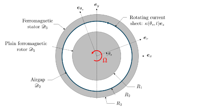
Figure 1: Cross-section of the simplified electric motor, indicating rotor, airgap and stator domains and corresponding frames.

The cross-section of the simplified induction motor is shown in Figure 1; the motor is considered infinitely long in the normal to the plane and under plane strain conditions. It is composed of a cylindrical ferromagnetic rotor (domain $\mathcal{D}_{1}:0\leq r\leq R_{1}$), surrounded by a cylindrical tubular stator (domain $\mathcal{D}_{3}:\ R_{2}\leq r\leq R_{3}$), separated by an airgap (domain $\mathcal{D}_{2}:\ R_{1}\leq r\leq R_{2}$). Two different polar coordinate systems are used: the stator’s fixed reference frame $\mathcal{S}(r,\theta_{s},z)$ and the rotor’s moving frame $\mathcal{R}(r,\theta,z)$, where $\theta\equiv\theta_{s}-\Omega t$, with $\Omega$ the clockwise angular velocity of the rotor, as shown in Figure 1.

Following Lubin et al. (2011), the motor is loaded by a current sheet of surface density $\boldsymbol{\kappa}$ perpendicular to the plane located on the internal radius of the stator. This current sheet models typical stator coils or windings supplied by a poly-phased (usually three-phased) alternating electric current of angular frequency $\omega$. The coils or windings are organized in $p$ pairs per phase and the applied surface current density is

$$\boldsymbol{\kappa}=\kappa_{0}\cos(p\theta_{s}-\omega t)\boldsymbol{e}_{z}\;,$$ (3.1)

with $\kappa_{0}$ the oscillation’s amplitude in $A/m$. This current sheet rotates around the $z$-axis at the angular frequency $\omega/p$. It creates a rotating magnetic field of the same angular frequency, which triggers induced currents at the rotor. The interaction of the induced currents in the rotor with the magnetic field create Lorentz forces that result in the rotor spinning at an angular frequency $\Omega$. Given that the phenomenon relies on induction, an angular frequency differential exists between the stator field and the rotor: $\Omega<{\omega}/{p}$. We thus define the relative angular frequency $\omega_{r}$ together with the slip parameter $s$

$$\omega_{r}=\omega-p\Omega\;;\quad s\equiv\frac{\omega_{r}}{\omega}\;,$$ (3.2)

where the angular velocities $\omega$ and $\Omega$ are constants, since the steady-state response of the motor is modeled.

Some additional assumptions are necessary to solve the problem.

i) Infinite permeability, rigid stator It is assumed that the stator’s strains are negligible – thus guaranteeing a constant radius current sheet – and that it has an infinite permeability, i.e. $\mu_{3}\longrightarrow\infty$, resulting in a negligible stator $h$-field

$$r>R_{2}:\ \boldsymbol{h}_{3}=({\scriptstyle\boldsymbol{\nabla}}\!\times\!\boldsymbol{a}_{3})/\mu_{3}\approx{\boldsymbol{0}}\;.$$ (3.3)

ii) Constant temperature airgap The air in the airgap is assumed to be maintained at a constant temperature $T_{a}$ by forced ventilation. Due to ohmic losses the rotor temperature rises, but a convective heat exchange discharges its excess heat in the airgap. The corresponding radiation condition is

$$r=R_{1}:\ \boldsymbol{q}\!\boldsymbol{\cdot}\!\boldsymbol{e}_{r}=-k({\scriptstyle\boldsymbol{\nabla}}T)\!\boldsymbol{\cdot}\!\boldsymbol{e}_{r}=h_{c}(T(R_{1})-T_{a})\;,$$ (3.4)

where $h_{c}$ is the convection coefficient and $T$ is the rotor temperature field.

iii) No external mechanical body forces No purely mechanical body forces, introduced in (2.7) are considered, i.e. $\boldsymbol{f}=\boldsymbol{0}$, since gravity effects are assumed negligible compared to inertia and magnetic contributions.

iv) Constant velocity and acceleration Assuming a small slip $s$ ($\omega_{r}\ll\Omega$) and a small vibration amplitude, we can ignore the rates of the displacement $\overset{\boldsymbol{.}}{\boldsymbol{u}}$ and $\overset{\boldsymbol{..}}{\boldsymbol{u}}$ in the velocity and acceleration terms, by keeping only their $\Omega$-dependent contributions, thus considerably simplifying the resulting algebra

$$\overset{\boldsymbol{.}}{\boldsymbol{x}}\approx r\Omega\boldsymbol{e}_{\theta}\;,\quad\overset{\boldsymbol{..}}{\boldsymbol{x}}\approx-r\Omega^{2}\boldsymbol{e}_{r}\;.$$ (3.5)

One consequence is a constant inertia term $-\rho_{0}r\Omega^{2}\boldsymbol{e}_{r}$ in the linear moment balance (2.20). The other consequence of (3.5)₁ are the simpler expressions of the electromotive intensity $\mathbcal{e}$ defined in (2.10) and the material time derivative $\dot{T}$, when expressed in the moving rotor frame (recall $\theta\equiv\theta_{s}-\Omega t$)

$$\begin{array}[]{rlll}\mathbcal{e}&=\displaystyle\left[-\frac{\partial\boldsymbol{a}}{\partial t}+\overset{\boldsymbol{.}}{\boldsymbol{x}}\!\times\!{\boldsymbol{b}}\right]_{\mathcal{S}}&=\displaystyle-\left[\frac{\partial\boldsymbol{a}}{\partial t}+\Omega\frac{\partial\boldsymbol{a}}{\partial{\theta_{s}}}\right]_{\mathcal{S}}&=\displaystyle-\frac{\partial\boldsymbol{a}}{\partial t}\bigg{|}_{\mathcal{R}}\;,\vspace{0.2cm}\\ \dot{T}&=\displaystyle\left[\frac{\partial T}{\partial t}+\overset{\boldsymbol{.}}{\boldsymbol{x}}\!\boldsymbol{\cdot}\!({\scriptstyle\boldsymbol{\nabla}}T)\right]_{\mathcal{S}}&=\ \ \ \!\displaystyle\left[\frac{\partial T}{\partial t}+\Omega\frac{\partial T}{\partial{\theta_{s}}}\right]_{\mathcal{S}}&=\ \ \displaystyle\frac{\partial T}{\partial t}\bigg{|}_{\mathcal{R}}\;.\end{array}$$ (3.6)

Henceforth all equations are written in the rotor frame $\mathcal{R}$ and all field quantities are functions of $(r,\theta,t)$. These governing equations and boundary conditions for the idealized, 2D motor are summarized below.

$$\begin{array}[]{rl}(r,\theta)\in{\mathcal{D}}_{1}:&\!\!\!\!{\scriptstyle\boldsymbol{\nabla}}\!\times\!\boldsymbol{b}=\mu\gamma\mathbcal{e}\;;\quad(R_{1},\theta):\boldsymbol{e}_{r}\!\times\!\left\llbracket\boldsymbol{h}\right\rrbracket=\boldsymbol{0}\;,\ \boldsymbol{e}_{r}\!\boldsymbol{\cdot}\!\left\llbracket\boldsymbol{b}\right\rrbracket=\boldsymbol{0}\;,\vspace{0.2cm}\\ (r,\theta)\in{\mathcal{D}}_{2}:&\!\!\!\!{\scriptstyle\boldsymbol{\nabla}}\!\times\!\boldsymbol{b}={\boldsymbol{0}}\;;\quad(R_{2},\theta):\boldsymbol{e}_{r}\!\times\!\boldsymbol{h}=\boldsymbol{\kappa}\;,\ {\boldsymbol{\kappa}}=\kappa_{0}\cos(p\theta-\omega_{r}t)\boldsymbol{e}_{z}\;,\vspace{0.2cm}\\ (r,\theta)\in{\mathcal{D}}_{1}:&\!\!\!\!\displaystyle\rho_{0}c_{\epsilon}{{\partial T}\over{\partial t}}-k{\scriptstyle\boldsymbol{\nabla}}^{2}T=\gamma\mathbcal{e}\!\boldsymbol{\cdot}\!\mathbcal{e}\;;\quad(R_{1},\theta):\boldsymbol{e}_{r}\!\boldsymbol{\cdot}\![k({\scriptstyle\boldsymbol{\nabla}}T)]=-h_{c}(T-T_{a})\;,\vspace{0.2cm}\\ (r,\theta)\in{\mathcal{D}}_{1}:&\!\!\!\!\displaystyle{\scriptstyle\boldsymbol{\nabla}}\!\boldsymbol{\cdot}\!(\overset{e}{\boldsymbol{\sigma}}+\overset{m}{\boldsymbol{\sigma}})=-\rho_{0}r\Omega^{2}\boldsymbol{e}_{r}\;;\quad(R_{1},\theta):\boldsymbol{e}_{r}\!\boldsymbol{\cdot}\!({\boldsymbol{\overset{e}{\boldsymbol{\sigma}}}}+\left\llbracket\boldsymbol{\overset{m}{\boldsymbol{\sigma}}}\right\rrbracket)={\boldsymbol{0}}\;,\vspace{0.2cm}\\ (r,\theta)\in{\mathcal{D}}_{1}\cup{\mathcal{D}}_{2}:&\!\!\!\!\boldsymbol{a}=a(r,\theta,t)\boldsymbol{e}_{z}\;,\ \mathbcal{e}=\displaystyle-\frac{\partial\boldsymbol{a}}{\partial t}\;,\ \boldsymbol{b}={\scriptstyle\boldsymbol{\nabla}}\!\times\!\boldsymbol{a}=\frac{1}{r}\frac{\partial a}{\partial\theta}\boldsymbol{e}_{r}-\frac{\partial a}{\partial r}\boldsymbol{e}_{\theta}\;.\end{array}$$ (3.7)

In the boundary condition for the equilibrium equation (3.7)₄ there is no elastic stress field in the airgap $\overset{e}{\boldsymbol{\sigma}}=\boldsymbol{0}$, in contrast to the magnetic stress field $\overset{m}{\boldsymbol{\sigma}}$ that exists in both the rotor and the airgap.

v) External torque applied at rotor’s center To balance the moment produced by the shear stresses, it is assumed that an external mechanical torque is applied at the center line of the rotor ($r=0$) along the $z$-axis. The resulting torque per unit rotor length $\mathcal{T}\boldsymbol{e}_{z}$ is

$$\mathcal{T}=r^{2}\int_{0}^{2\pi}\sigma_{r\theta}(r,\theta)\mathrm{d}\theta\;,$$ (3.8)

and will be shown to be a constant, function of the relative angular frequency $\mathcal{T}(\omega_{r})$ with $\mathcal{T}(0)=0$.

3.2 Dimensionless boundary value problem

To guide the physical interpretation of the results, the following dimensionless variables and parameters of the problem are introduced

$$\frac{r}{R_{1}}\rightarrow r,\quad\omega_{r}t\rightarrow t,\quad\frac{a}{\mu_{0}\kappa_{0}R_{1}}\rightarrow a,\quad\frac{k(T-T_{a})}{\gamma\omega_{r}^{2}(\mu_{0}\kappa_{0})^{2}R_{1}^{4}}\rightarrow T,\quad\frac{\boldsymbol{\sigma}}{\rho_{0}R_{1}^{2}\Omega^{2}}\rightarrow\boldsymbol{\sigma},\quad\zeta\equiv(R_{2}-R_{1})/R_{1}\;.$$ (3.9)

Henceforth, for simplicity the dimensionless variables and field quantities of the problem, $r,\;t,\;a,\;T,\;\boldsymbol{\sigma}$ are denoted by the same symbol as their dimensioned counterparts.

The governing equations and the associated interface and boundary conditions (in the rotor frame) are given below, starting with the magnetic potential $a$

$$\begin{array}[]{ll}\vspace{0.2cm}{\scriptstyle\boldsymbol{\nabla}}^{2}a_{1}=\alpha^{2}\displaystyle\frac{\partial a_{1}}{\partial t}\;,\quad\alpha^{2}\equiv\mu\gamma\omega_{r}R_{1}^{2}\;;&0\leq r\leq 1\;,\\ \vspace{0.2cm}\displaystyle\frac{\partial a_{1}}{\partial r}=(1+\chi)\frac{\partial a_{2}}{\partial r}\;,\quad\frac{\partial a_{1}}{\partial\theta}=\frac{\partial a_{2}}{\partial\theta}\;;&r=1\;,\\ \vspace{0.2cm}{\scriptstyle\boldsymbol{\nabla}}^{2}a_{2}=0\;;&1\leq r\leq 1+\zeta\;,\\ \vspace{0.2cm}\displaystyle\frac{\partial a_{2}}{\partial r}=\cos(p\theta-t)\;;&r=1+\zeta\;.\end{array}$$ (3.10)

The governing equation and boundary condition for the rotor’s temperature field $T$ are

$$\begin{array}[]{ll}\vspace{0.2cm}\displaystyle{\mathcal{F}}^{-1}\frac{\partial T}{\partial t}-{\scriptstyle\boldsymbol{\nabla}}^{2}T=\left(\frac{\partial a_{1}}{\partial t}\right)^{2}\;,\quad{{\mathcal{F}}}\equiv\frac{k}{\rho_{0}c_{\epsilon}\omega_{r}R_{1}^{2}}\;;&0\leq r\leq 1\;,\\ \displaystyle{\mathcal{B}}\frac{\partial T}{\partial r}+T=0\;,\quad{\mathcal{B}}\equiv\frac{k}{R_{1}h_{c}}\;;&r=1\;,\end{array}$$ (3.11)

with ${\mathcal{F}}$ and ${\mathcal{B}}$ the “Fourier” and “Biot” dimensionless coefficients respectively.

Finally, the governing equations and boundary conditions for the rotor’s elastic stress field $\overset{e}{\boldsymbol{\sigma}}$ are

$$\begin{array}[]{ll}\displaystyle{\scriptstyle\boldsymbol{\nabla}}\!\boldsymbol{\cdot}\!{\overset{e}{\boldsymbol{\sigma}}}={\boldsymbol{f}}\;,\quad{\boldsymbol{f}}\equiv s_{j}\alpha^{2}\frac{\partial\boldsymbol{a}_{1}}{\partial t}\!\times\!({\scriptstyle\boldsymbol{\nabla}}\!\times\!\boldsymbol{a}_{1})-s_{m}{\scriptstyle\boldsymbol{\nabla}}\left(\|{\scriptstyle\boldsymbol{\nabla}}\!\times\!\boldsymbol{a}_{1}\|^{2}\right)-r\boldsymbol{e}_{r}\;;&0\leq r\leq 1\;,\vspace{0.2cm}\\ \displaystyle s_{j}\equiv s_{0}\frac{1+\Lambda}{1+\chi}\;,\quad s_{m}\equiv{s_{0}\over 2}{{\chi+\Lambda}\over{1+\chi}}\;,\quad s_{0}\equiv\frac{\mu_{0}\kappa_{0}^{2}}{\rho_{0}R_{1}^{2}\Omega^{2}}\;.&\vspace{0.2cm}\\ \displaystyle\overset{e}{\sigma}_{rr}=\frac{s_{0}}{2}\left[\left(\frac{\partial a_{2}}{\partial\theta}\right)^{2}-\left({\frac{\partial a_{2}}{\partial r}}\right)^{2}\right]-(\frac{s_{j}}{2}+s_{m})\left(\frac{\partial a_{1}}{\partial\theta}\right)^{2}+(\frac{s_{j}}{2}-s_{m})\left({\frac{\partial a_{1}}{\partial r}}\right)^{2}\;;&r=1\;,\vspace{0.2cm}\\ \displaystyle\overset{e}{\sigma}_{r\theta}=-s_{0}\frac{\partial a_{2}}{\partial\theta}{\frac{\partial a_{2}}{\partial r}}+s_{j}\frac{\partial a_{1}}{\partial\theta}{\frac{\partial a_{1}}{\partial r}}\;;&r=1\;.\end{array}$$ (3.12)

$s_{0}$ is an equivalent of the “Stuart” number for magnetic fluids and gives the ratio of Maxwell over inertia stress magnitudes. The dimensionless coefficients $s_{j}$ and $s_{m}$ appearing in the expressions for the total stress in the rotor ${\boldsymbol{\sigma}}_{1}$ (sum of the elastic $\overset{e}{\boldsymbol{\sigma}}$ and the magnetic $\overset{m}{\boldsymbol{\sigma}}$ components respectively) depend on its magnetic properties while the total stress tensor in the airgap ${\boldsymbol{\sigma}}_{2}$ (Maxwell stress in vacuum) depends only on $s_{0}$. The corresponding expressions for the magnetic field and the total stress in each domain are given by

$$\begin{array}[]{ll}\displaystyle{\boldsymbol{\sigma}}_{1}=\overset{e}{\boldsymbol{\sigma}}+\overset{m}{\boldsymbol{\sigma}}\;,\ \overset{m}{\boldsymbol{\sigma}}=\displaystyle s_{j}\boldsymbol{b}_{1}\boldsymbol{b}_{1}+(s_{m}-{s_{j}\over 2})(\boldsymbol{b}_{1}\!\boldsymbol{\cdot}\!\boldsymbol{b}_{1})\boldsymbol{I}\;,\quad{\boldsymbol{b}}_{1}={\scriptstyle\boldsymbol{\nabla}}\!\times\!{\boldsymbol{a}}_{1}\;;&0\leq r\leq 1\;,\vspace{0.2cm}\\ {\boldsymbol{\sigma}}_{2}=\overset{m}{\boldsymbol{\sigma}}=\displaystyle s_{0}[\boldsymbol{b}_{2}\boldsymbol{b}_{2}-\frac{1}{2}(\boldsymbol{b}_{2}\!\boldsymbol{\cdot}\!\boldsymbol{b}_{2})\boldsymbol{I}]\;,\quad{\boldsymbol{b}}_{2}={\scriptstyle\boldsymbol{\nabla}}\!\times\!{\boldsymbol{a}}_{2}\;;&1\leq r\leq 1+\zeta\;.\end{array}$$ (3.13)

We first solve (3.10) to find the magnetic potential $a$, thus obtaining the ohmic dissipation for the heat equation (3.11), which is then used to determine the rotor’s temperature field $T$. The magnetic potential gives the body forces for the linear momentum balance in (3.12), thus providing the rotor’s elastic field $\overset{e}{\boldsymbol{\sigma}}$.

3.3 Magnetic Potential

Solving the linear problem in (3.10) subject to the harmonic loading in (3.1), is more efficiently done in the complex domain, where the magnetic potential $a_{k}(r,\theta,t)$ takes the form

$$a_{k}(r,\Theta)=\Re\left\{{\bar{a}}_{k}(r)\exp(-i\Theta)\right\}=A_{k}(r)\cos\Theta+B_{k}(r)\sin\Theta\;,\ k=1,2\;;\quad\Theta\equiv p\theta-t\;,$$ (3.14)

where ${\bar{a}}_{k}(r)=A_{k}(r)+iB_{k}(r)$ is the complex magnetic potential amplitude that depends only on $r$.

In the rotor domain, (3.10) results in a Bessel differential equation for the complex amplitude ${\bar{a}}_{1}(r)$

$$r^{2}\frac{\mathrm{d}^{2}{\bar{a}}_{1}}{\mathrm{d}r^{2}}+r\frac{\mathrm{d}{\bar{a}}_{1}}{\mathrm{d}r}+({{\bar{\alpha}}}^{2}r^{2}-p^{2}){\bar{a}}_{1}=0\ \Longrightarrow\ {\bar{a}}_{1}(r)={\bar{A}}J_{p}({\bar{\alpha}}r)\;;\quad{{\bar{\alpha}}}^{2}\equiv-i\alpha^{2}\;,$$ (3.15)

where the constant $\alpha^{2}$ is defined in (3.10) and $J_{p}$ denotes a Bessel function of the first kind. The above expression for ${\bar{a}}_{1}$ accounts for the fact that there is no singularity in $r=0$, and hence explains the absence of a Bessel function of the second kind in the general solution.

In the airgap domain, (3.10) gives a Laplace equation for the complex amplitude ${\bar{a}}_{2}(r)$

$$r^{2}\frac{\mathrm{d}^{2}{\bar{a}}_{2}}{\mathrm{d}r^{2}}+r\frac{\mathrm{d}{\bar{a}}_{2}}{\mathrm{d}r}-p^{2}{\bar{a}}_{2}=0\ \Longrightarrow\ {\bar{a}}_{2}(r)={\bar{B}}r^{p}+{\bar{C}}r^{-p}\;.$$ (3.16)

The complex-valued constants ${\bar{A}}$, ${\bar{B}}$ and ${\bar{C}}$ appearing in (3.15) and (3.16) are determined using the interface and boundary conditions in (3.10), and are found to be

$$\begin{array}[]{l}\vspace{0.2cm}\displaystyle{\bar{A}}={{2\mathcal{h}}\over{J_{p}({\bar{\alpha}})+{\bar{\mathcal{g}}}}}\;,\\ \vspace{0.2cm}\displaystyle{\bar{B}}=\mathcal{h}\left[1-{{2{\bar{\mathcal{g}}}}\over[J_{p}({\bar{\alpha}})+{\bar{\mathcal{g}}}][1+(1+\zeta)^{-2p}]}\right]\;,\\ \vspace{0.2cm}\displaystyle{\bar{C}}=\mathcal{h}\left[1-{{2{\bar{\mathcal{g}}}}\over[J_{p}({\bar{\alpha}})+{\bar{g}}][1+(1+\zeta)^{2p}]}\right]\;,\\ \displaystyle{\bar{\mathcal{g}}}\equiv\left[{J_{p}({\bar{\alpha}})-\displaystyle{{{\bar{\alpha}}}\over{p}}J_{p+1}({\bar{\alpha}})}\right]\left[{{(1+\zeta)^{p}+(1+\zeta)^{-p}}\over{(1+\zeta)^{p}-(1+\zeta)^{-p}}}\right]{1\over{1+\chi}}\;,\quad\mathcal{h}\equiv{{(1+\zeta)}\over{p[(1+\zeta)^{p}-(1+\zeta)^{-p}]}}\;.\end{array}$$ (3.17)

Using (3.17), the sought real amplitudes $A_{k}(r)$ and $B_{k}(r)$ in (3.14) are given in terms of their complex counterparts found in (3.15) and (3.16), i.e. $A_{k}(r)=\Re\left\{{\bar{a}}_{k}(r)\right\},\ B_{k}(r)=\Im\left\{{\bar{a}}_{k}(r)\right\};\ k=1,2$.

3.4 Rotor temperature

From the linearity of the governing equations for the temperature field in (3.11) and the magnetic potential solution in the rotor in (3.15), the forcing term in the conduction equation is found to be: $(\partial a_{1}/\partial t)^{2}=0.5[(B_{1}(r))^{2}+(A_{1}(r))^{2}]+0.5[(B_{1}(r))^{2}-(A_{1}(r))^{2}]\cos(2\Theta)-A_{1}(r)B_{1}(r)\sin(2\Theta)$. The use of superposition and complex formulation lead to the following rotor temperature field $T(r,\theta,t)$

$$T(r,\Theta)=T_{0}(r)+\Re\left\{{{\bar{T}}}(r)\exp(-i2\Theta)\right\}\;;\quad\Theta\equiv p\theta-t\;,$$ (3.18)

where the function $T_{0}(r)$ is real and ${{\bar{T}}}(r)$ is complex. The real function $T_{0}(r)$ is found from (3.11) to be

$$\frac{\mathrm{d}^{2}T_{0}}{\mathrm{d}r^{2}}+\frac{1}{r}\frac{\mathrm{d}T_{0}}{\mathrm{d}r}=-{{B_{1}}^{2}(r)+{A_{1}}^{2}(r)\over{2}}\ \Longrightarrow\ T_{0}(r)=c_{0}-\frac{1}{2}\int_{0}^{r}\left(\frac{1}{r}\int_{0}^{r}[B_{1}^{2}+A_{1}^{2}]r\mathrm{d}r\right)\mathrm{d}r\;,$$ (3.19)

with the unknown constant $c_{0}$ to be determined from the boundary condition.

Solving for the complex function ${\bar{T}}(r)$ is reduced to solving a Bessel differential equation with a forcing term through the superposition of a homogeneous and a particular solution ${\bar{T}}_{p}(r)$, as follows

$$\begin{array}[]{l}\vspace{0.2cm}\displaystyle r^{2}\frac{\mathrm{d}^{2}{\bar{T}}}{\mathrm{d}r^{2}}+r\frac{\mathrm{d}{\bar{T}}}{\mathrm{d}r}+\left({{\bar{\beta}}}^{2}r^{2}-(2p)^{2}\right){\bar{T}}=r^{2}\frac{{{\bar{a}}_{1}}^{2}}{2}\quad\Longrightarrow\quad{\bar{T}}(r)={\bar{c}}J_{2p}({\bar{\beta}}r)+{\bar{T}}_{p}(r)\;;\quad{{\bar{\beta}}}^{2}\equiv-\frac{2i}{\mathcal{F}}\;,\\ {\bar{T}}_{p}(r)=\displaystyle{\pi\over 4}\left[-J_{2p}({\bar{\beta}}r)\int_{0}^{r}Y_{2p}({\bar{\beta}}r){{\bar{a}}_{1}}^{2}r\mathrm{d}r+Y_{2p}({\bar{\beta}}r)\int_{0}^{r}J_{2p}({\bar{\beta}}r){{\bar{a}}_{1}}^{2}r\mathrm{d}r\right]\;,\end{array}$$ (3.20)

where the unknown constant ${\bar{c}}$ in the homogeneous part of the solution will be specified from the boundary condition. In solving (3.20) we made use of the fact that the solution is bounded at $r=0$, and hence there is no contribution from the Bessel function of the second kind $Y_{2p}$ to the homogeneous part of the solution. However, $Y_{2p}$ does enter under the integrals in the expressions for the particular solution ${\bar{T}}_{p}(r)$ as seen above.

Finally, the boundary condition at $r=1$ in (3.11) splits into two boundary conditions: one for $T_{0}(r)$ that gives $c_{0}$ and the other for ${\bar{T}}(r)$ that provides ${\bar{c}}$

$$\begin{array}[]{l}\vspace{0.2cm}c_{0}=\displaystyle\frac{1}{2}\left[\int_{0}^{1}\left(\frac{1}{r}\int_{0}^{r}[(B_{1}(r))^{2}+(A_{1}(r))^{2}]r\mathrm{d}r\right)\mathrm{d}r+{\mathcal{B}}\int_{0}^{1}[(B_{1}(r))^{2}+(A_{1}(r))^{2}]r\mathrm{d}r\right]\;,\\ {\bar{c}}=\displaystyle{\pi\over 4}\left[\int_{0}^{1}Y_{2p}({\bar{\beta}}r){{\bar{a}}_{1}}^{2}(r)r\mathrm{d}r-{{Y_{2p}({\bar{\beta}})+{\mathcal{B}}{\bar{\beta}}Y^{\prime}_{2p}({\bar{\beta}})}\over{J_{2p}({\bar{\beta}})+{\mathcal{B}}{\bar{\beta}}J^{\prime}_{2p}({\bar{\beta}})}}\int_{0}^{1}J_{2p}({\bar{\beta}}r){{\bar{a}}_{1}}^{2}(r)r\mathrm{d}r\right]\;,\end{array}$$ (3.21)

where $J^{\prime}_{2p}$ and $Y^{\prime}_{2p}$ denote the derivatives of the first and second kind Bessel functions of order $2p$ with respect to their argument.

Having determined $T_{0}(r)$ and ${\bar{T}}(r)$, one can find from (3.18) the rotor temperature field $T(r,\Theta)$.

3.5 Rotor stresses

The principle of superposition is used again for determining the rotor’s elastic stress field $\overset{e}{\boldsymbol{\sigma}}$. Recalling the definitions for $\boldsymbol{f}$ in (3.12) and the solution for the magnetic potential $a_{1}$ in (3.14) and (3.15), the body forces can be expressed as $\boldsymbol{f}(r,\Theta)=\boldsymbol{N}(r)+{\scriptstyle\boldsymbol{\nabla}}V(r,\Theta)$, where $\boldsymbol{N}(r)$ is not derivable from a potential (non-conservative part of the force field), while the remaining terms are derivable from a potential $V(r,\Theta)$.

$$\begin{array}[]{rl}\vspace{0.2cm}\boldsymbol{f}=&\!\!\!\!\displaystyle\boldsymbol{N}+{\scriptstyle\boldsymbol{\nabla}}V\;;\\ \vspace{0.2cm}\boldsymbol{N}=&\!\!\!\!\displaystyle-\frac{s_{j}\alpha^{2}}{2}\frac{p}{r}(A_{1}^{2}+B_{1}^{2})\boldsymbol{e}_{\theta}\;;\ V(r,\Theta)=V_{0}(r)+V_{cs}(r,\Theta)\;,\ V_{cs}=V_{s}(r)\sin(2\Theta)+V_{c}(r)\cos(2\Theta)\;,\\ \vspace{0.2cm}V_{0}(r)=&\!\!\!\!\displaystyle-{r^{2}\over 2}+\frac{s_{j}\alpha^{2}}{2}\int_{0}^{r}(A_{1}B_{1}^{\prime}-A_{1}^{\prime}B_{1})\mathrm{d}r-\frac{s_{m}}{2}\left(\frac{p^{2}}{r^{2}}(A_{1}^{2}+B_{1}^{2})+(A_{1}^{\prime 2}+B_{1}^{\prime 2})\right)\;,\\ \vspace{0.2cm}V_{c}(r)=&\!\!\!\!\displaystyle-\frac{s_{j}\alpha^{2}}{2}A_{1}B_{1}-\frac{s_{m}}{2}\left(\frac{p^{2}}{r^{2}}(B_{1}^{2}-A_{1}^{2})+(A_{1}^{\prime 2}-B_{1}^{\prime 2})\right)\;,\\ \vspace{0.2cm}V_{s}(r)=&\!\!\!\!\displaystyle\frac{s_{j}\alpha^{2}}{2}\frac{(A_{1}^{2}-B_{1}^{2})}{2}-s_{m}\left(\frac{p^{2}}{r^{2}}A_{1}B_{1}+A_{1}^{\prime}B_{1}^{\prime}\right)\;.\end{array}$$ (3.22)

Consequently, the rotor’s elastic stress field $\overset{e}{\boldsymbol{\sigma}}$ is decomposed as follows

$$\overset{e}{\boldsymbol{\sigma}}(r,\Theta)=\overset{e}{\boldsymbol{\sigma}}^{{}_{N}}(r)+\overset{e}{\boldsymbol{\sigma}}^{{}_{V}}(r,\Theta)+\overset{e}{\boldsymbol{\sigma}}^{{}_{h}}(r,\Theta)\;,\quad\left\{\begin{split}&{\scriptstyle\boldsymbol{\nabla}}\!\boldsymbol{\cdot}\!\overset{e}{\boldsymbol{\sigma}}^{{}_{N}}=\boldsymbol{N}\;,\\ &{\scriptstyle\boldsymbol{\nabla}}\!\boldsymbol{\cdot}\!\overset{e}{\boldsymbol{\sigma}}^{{}_{V}}={\scriptstyle\boldsymbol{\nabla}}V\;,\\ &{\scriptstyle\boldsymbol{\nabla}}\!\boldsymbol{\cdot}\!\overset{e}{\boldsymbol{\sigma}}^{{}_{h}}={\boldsymbol{0}}\;,\end{split}\right.$$ (3.23)

where each one of the constituent fields $\overset{e}{\boldsymbol{\sigma}}^{{}_{N}},\;\overset{e}{\boldsymbol{\sigma}}^{{}_{V}},\;\overset{e}{\boldsymbol{\sigma}}^{{}_{h}}$ corresponds, in view of (2.25), to a compatible elastic strain field, i.e. derivable from a displacement field. By abuse of terminology we call these elastic stress fields elastically compatible.

Using the expression for $\boldsymbol{N}(r)$ from (3.22), an elastically compatible particular solution for $\overset{e}{\boldsymbol{\sigma}}^{{}_{N}}(r)$ is found by solving the tangential equilibrium ODE,

$$\begin{array}[]{l}\vspace{0.2cm}\displaystyle\frac{\mathrm{d}\overset{e}{\sigma}^{{}_{N}}_{r\theta}}{\mathrm{d}r}+\frac{2}{r}\overset{e}{\sigma}^{{}_{N}}_{r\theta}=-\frac{s_{j}\alpha^{2}}{2}\frac{p}{r}(A_{1}^{2}+B_{1}^{2})\ \Longrightarrow\ \overset{e}{\sigma}^{{}_{N}}_{r\theta}=-\frac{s_{j}\alpha^{2}}{2}\frac{p}{r^{2}}\int_{0}^{r}r(A_{1}^{2}+B_{1}^{2})\mathrm{d}r\;.\end{array}$$ (3.24)

An elastically compatible particular solution for the elastic stress field $\overset{e}{\boldsymbol{\sigma}}^{{}_{V}}$ is found using the Airy stress function method in polar coordinates (see Barber (2009)). The components of $\overset{e}{\boldsymbol{\sigma}}^{{}_{V}}$ can be expressed in terms of a stress potential $\phi_{{}_{V}}$ as follows

$$\overset{e}{\sigma}^{{}_{V}}_{rr}=\frac{1}{r}\frac{\partial\phi_{{}_{V}}}{\partial r}+\frac{1}{r^{2}}\frac{\partial^{2}\phi_{{}_{V}}}{\partial\Theta^{2}}+V\;,\ \overset{e}{\sigma}^{{}_{V}}_{\theta\theta}=\frac{\partial^{2}\phi_{{}_{V}}}{\partial r^{2}}+V\;,\ \overset{e}{\sigma}^{{}_{V}}_{r\theta}=-\frac{\partial}{\partial r}\left(\frac{1}{r}\frac{\partial\phi_{{}_{V}}}{\partial\Theta}\right)\;;\quad\displaystyle\nabla^{2}\phi_{{}_{V}}=-{{1-2\nu}\over{1-\nu}}V\;.$$ (3.25)

The stress potential $\phi_{{}_{V}}$ is found (see footnote 17), by solving the Laplacian in (3.25) with the help of (3.22)

$$\phi_{{}_{V}}(r,\Theta)=-{{1-2\nu}\over{1-\nu}}\left(\int_{0}^{r}\frac{1}{r}\int_{0}^{r}V_{0}r\mathrm{d}r\ \mathrm{d}r+\frac{r^{2p}}{4p}\int_{0}^{r}V_{cs}r^{-2p+1}\mathrm{d}r-\frac{r^{-2p}}{4p}\int_{0}^{r}V_{cs}r^{2p+1}\mathrm{d}r\right)\;.$$ (3.26)

The components of the elastically compatible homogeneous solution stress field $\overset{e}{\boldsymbol{\sigma}}^{{}_{h}}$ are expressed in terms of the potential $\phi_{h}$

$$\overset{e}{\sigma}^{{}_{h}}_{rr}=\frac{1}{r}\frac{\partial\phi_{{}_{h}}}{\partial r}+\frac{1}{r^{2}}\frac{\partial^{2}\phi_{{}_{h}}}{\partial\Theta^{2}}\;,\ \overset{e}{\sigma}^{{}_{h}}_{\theta\theta}=\frac{\partial^{2}\phi_{{}_{h}}}{\partial r^{2}}\;,\ \overset{e}{\sigma}^{{}_{V}}_{r\theta}=-\frac{\partial}{\partial r}\left(\frac{1}{r}\frac{\partial\phi_{{}_{V}}}{\partial\Theta}\right)\;;\quad\displaystyle\nabla^{4}\phi_{{}_{h}}=0\;.$$ (3.27)

Solving the biharmonic equation for $\phi_{{}_{h}}$ in (3.27) we obtain

$$\phi_{h}(r,\Theta)=\Phi_{01}\frac{r^{2}}{2}+\Phi_{02}\theta+\left(\Phi_{c1}r^{2p}+\Phi_{c2}r^{2p+2}\right)\cos(2\Theta)+\left(\Phi_{s1}r^{2p}+\Phi_{s2}r^{2p+2}\right)\sin(2\Theta)\;.$$ (3.28)

The final expressions for $\overset{e}{\boldsymbol{\sigma}}^{{}_{h}},\overset{e}{\boldsymbol{\sigma}}^{{}_{V}}$ are obtained from (3.27) and (3.27). The six constants $\Phi_{01},\Phi_{02},\Phi_{c1},\Phi_{c2},\Phi_{s1},\Phi_{s2}$ are determined by the $r=1$ boundary conditions in (3.12)

$$\begin{array}[]{ll}\displaystyle\overset{e}{\sigma}^{{}_{V}}_{rr}(1)+\overset{e}{\sigma}^{{}_{h}}_{rr}(1)=\frac{s_{0}}{2}\left[\left(\frac{\partial a_{2}}{\partial\theta}\right)^{2}-\left({\frac{\partial a_{2}}{\partial r}}\right)^{2}\right]-(\frac{s_{j}}{2}+s_{m})\left(\frac{\partial a_{1}}{\partial\theta}\right)^{2}+(\frac{s_{j}}{2}-s_{m})\left({\frac{\partial a_{1}}{\partial r}}\right)^{2}\;,\vspace{0.2cm}\\ \displaystyle\overset{e}{\sigma}^{{}_{N}}_{r\theta}(1)+\overset{e}{\sigma}^{{}_{V}}_{r\theta}(1)+\overset{e}{\sigma}^{{}_{h}}_{r\theta}(1)=-s_{0}\frac{\partial a_{2}}{\partial\theta}{\frac{\partial a_{2}}{\partial r}}+s_{j}\frac{\partial a_{1}}{\partial\theta}{\frac{\partial a_{1}}{\partial r}}\;.\end{array}$$ (3.29)

From the decomposition in radial, cosine and sine terms (see footnote 18), result three equations for the normal and three equations for the tangential boundary conditions, thus uniquely determining the sought constants. The full expressions for the stress at the rotor (elastic and magnetic components) can be then determined from (3.13) and (3.23) but are too cumbersome to be recorded here; the components of $\overset{e}{\boldsymbol{\sigma}}^{{}_{V}}$ and $\overset{e}{\boldsymbol{\sigma}}^{{}_{h}}$ are given in B.

3.6 Rotor torque

We are now in a position to give the expression for the torque/unit length $\mathcal{T}$. Recalling (3.8) and using the results for the stress field obtained above, one has

$$\mathcal{T}=4\pi\rho_{0}\Omega^{2}R_{1}^{4}s_{0}p\left(\frac{\mathcal{h}}{\|J_{p}({\bar{\alpha}})+\bar{\mathcal{g}}\|}\right)^{2}\Im\left\{J_{p}({\bar{\alpha}}){\bar{\alpha}}^{*}J_{p+1}({\bar{\alpha}})^{*}\right\}\;,$$ (3.30)

where $(\ )^{*}$ denotes complex conjugation. This result gives the torque in terms of geometry, applied current (poles, amplitude and frequency), magnetic and electric properties and density of the rotor. Remarkably, $\mathcal{T}$ is independent of the mechanical properties of the rotor, i.e. its shear modulus $G$ and Poisson ratio $\nu$.

As the torque is a function of slip velocity $\omega_{r}$, it is instructive to find from (3.30) the initial slope of the $\mathcal{T}(\omega_{r})$ curve. Using asymptotics of the Bessel functions with respect to ${\bar{\alpha}}$ for $\|{\bar{\alpha}}\|^{2}=\alpha^{2}=\omega_{r}\mu\gamma R_{1}^{2}<\!\!<1$, one obtains

$$\mathcal{T}\approx\omega_{r}{{2\pi\gamma}\over{p(1+p)}}\left[{{\mu_{0}\kappa_{0}(1+\chi)(1+\zeta)R_{1}}\over{(1+\zeta)^{p}+(1+\zeta)^{-p}+(1+\chi)[(1+\zeta)^{p}-(1+\zeta)^{-p}]}}\right]^{2}+O(\omega_{r})^{2}\;.$$ (3.31)

One should keep in mind that the above expression gives only the initial slope of the $\mathcal{T}(\omega_{r})$ curve, but depending on the problem, the range of validity of this linear approximation can be very small.

4 Results and discussion

Although we solve an idealized motor, the results presented here correspond to materials, geometries and operating parameters found in the electrical engineering literature. The dimensionless quantities introduced in (3.9) allow a direct comparison of the results to related physically meaningful quantities.

4.1 Material, geometry and operating parameters

The motor geometry and operating parameters used in the calculations are shown in Table 1. The study covers three materials typically found in electric motors: electrical steel, copper and aluminum. Despite the different motor architecture, the same values as in Lubin et al. (2011) are used whenever possible. The peak value of the current sheet is presently reduced to $1.3\!\times\!10^{4}A/m$ – from $8\!\times\!10^{4}A/m$ in Lubin et al. (2011) – in order to keep the maximum value of the magnetic field in the steel rotor below saturation, phenomenon not accounted for here.

Unfortunately, not all needed parameters can be found for a particular electric steel, thus requiring the use of experimental data from the open literature for comparable materials. The value for the magneto-mechanical coupling coefficient $\Lambda$ is fitted from Aydin et al. (2017), for the no-prestressed case, as detailed in C. A typical value for the magnetic susceptibility $\chi=4000$ for electric steel is adopted, while the elastic constants $\nu$ and $E$ are taken from Belahcen et al. (2006). The rest of the material parameters – not given in Belahcen et al. (2006) and Aydin et al. (2017) – are taken from the open literature, as it is also done for the case of copper and aluminum, where we assume negligible magnetic effects ($\chi=\Lambda=0$).

The base case motor, which serves as a benchmark, is made of electric steel, has an airgap parameter $\zeta=0.05$ and a slip parameter $s=0.02$. The rest of the geometric and operating parameters are kept fixed, independently of the rotor material, as shown below in Table 1.

Geometry
Rotor radius $R_{1}$	$6$ cm
Airgap parameter $\zeta=(R_{2}-R_{1})/R_{1}$	$0.05$ (base case)
Number of pole pairs $p$	2
Operating parameters
Peak value of current sheet $\kappa_{0}$	$1.3\!\times\!10^{4}$ A/m
Angular velocity of current supply $\omega$	$100\pi$ rad/s
Slip $s=\omega_{r}/\omega$	$2$% (base case)
External temperature $T_{a}$	$20^{\circ}$C
Convection coefficient $h_{c}$	$40$ W/m2/K
Material properties	Electrical steel	Copper	Aluminum
Electric conductivity $\gamma$	$2.67\!\times\!10^{6}$ S/m	$5.96\!\times\!10^{7}$ S/m	$3.5\!\times\!10^{7}$ S/m
Magnetic susceptibility $\chi$	$4,000$	$\approx 0$	$\approx 0$
Magneto-mechanical coupling $\Lambda$	$-1,800$	$\approx 0$	$\approx 0$
Mass density $\rho_{0}$	$7,650\ \text{kg/m}^{3}$	$8,940\ \text{kg/m}^{3}$	$2,700\ \text{kg/m}^{3}$
Young’s modulus $E$	$183\!\times\!10^{9}$ Pa	$117\!\times\!10^{9}$ Pa	$69\!\times\!10^{9}$ Pa
Poisson ratio $\nu$	$0.34$	$0.33$	$0.32$
Specific heat capacity $c_{\epsilon}$	$480$ J/kg/K	$385$  J/kg/K	$921$ J/kg/K
Thermal conductivity $k$	$45$ W/m/K	$397$  W/m/K	$225$  W/m/K

Table 1: Motor geometry, operating parameters and rotor material properties

As discussed in Subsection 3.1, the equations are solved in the rotor frame $\mathcal{R}$ and all field quantities are functions of $(r,\Theta)$, where $\Theta=p\theta-t$ and $p$ the motor pole number (here taken $p=2$). The results here are a snapshot of these rotating fields at $t=0$ and are presented by plotting the corresponding field quantity at $(r,\theta)$.

4.2 Magnetic field in rotor and airgap

Magnetic field calculations for realistic geometries are routine for the electrical engineering community. The results for the current simple motor geometry are presented here solely for the purpose of explaining the resulting force and strain fields.

The magnetic field plots in Figures 2 and 3 show the contours of the dimensionless (normalized by $\mu_{0}\kappa_{0}$) magnetic field $\|\boldsymbol{b}\|=(b_{r}^{2}+b_{\theta}^{2})^{1/2}$ for three different values of the slip parameter $s=0.02,\;0.05,\;0.10$ in the case of a steel rotor with an airgap parameter $\zeta=0.05$. Notice that the magnetic field increases away from the center and peaks in a localized zone near the rotor periphery. As the slip $s$ (equivalently the relative velocity $\omega_{r}$) increases, the localized high magnetization zone narrows, (e.g. see Jackson (1999) that the skin depth $\delta=(2/{\gamma\omega_{r}\mu})^{1/2}$). The four localized magnetic field zones are a result of the number of poles ($p=2$).

The high permeability of the rotor material ($\chi=4000$ for electric steel) drastically increases its magnetic field, thus masking the variations of the considerably smaller – by one order of magnitude – strength of the magnetic field in the airgap in Figures 2. To remedy this, Figure 3 shows only the airgap magnetic field (hiding the rotor magnetic field) for the $s=0.02$ slip motor of Figure 2(a).

(a) $\|\boldsymbol{b}\|$ for $s=0.02$

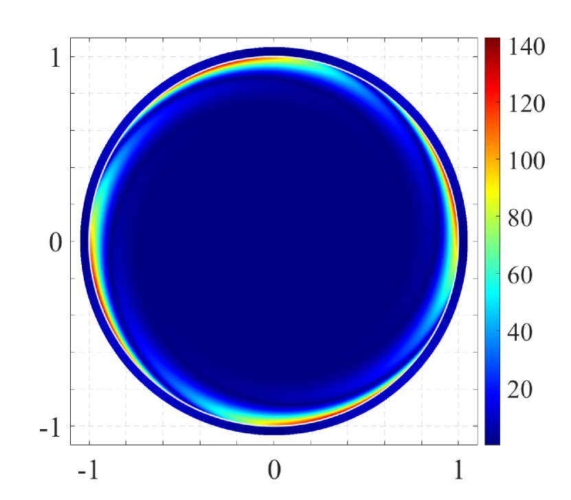
(b) $\|\boldsymbol{b}\|$ for $s=0.05$

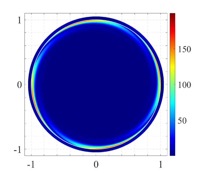
(c) $\|\boldsymbol{b}\|$ for $s=0.10$

Figure 2: Magnetic field norm $\|\boldsymbol{b}\|$ for a steel rotor (normalized by $\mu_{0}\kappa_{0}$), for different values of the slip parameter $s$.

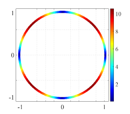
Figure 3: Magnetic field norm $\|\boldsymbol{b}\|$ in the airgap region (normalized by $\mu_{0}\kappa_{0}$) for the base case motor in Figure 2(a).

The influence of changing motor geometry is presented in Figure 4 for three different airgap parameters $\zeta=0,02,\;0.05,\;0.10$ in a steel rotor and a slip value $s=0.02$. As expected, Reducing the airgap size does not affect the distribution of the magnetic field, but increases drastically the maximum strength of the field.

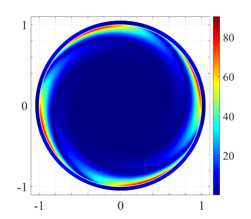
(a) $\|\boldsymbol{b}\|$ for $\zeta=0.02$

(b) $\|\boldsymbol{b}\|$ for $\zeta=0.05$

(c) $\|\boldsymbol{b}\|$ for $\zeta=0.10$

Figure 4: Magnetic field norm $\|\boldsymbol{b}\|$ for a steel rotor (normalized by $\mu_{0}\kappa_{0}$), for different values of the airgap parameter $\zeta$.

Comparison of the magnetic fields for different rotor materials is presented in Figure 5, where the results for the high magnetic susceptibility steel are contrasted to the non-magnetic copper and aluminum rotors. The slip and airgap parameters are kept at their default value $s=0.02$, $\zeta=0.05$.

(a) $\|\boldsymbol{b}\|$ – steel

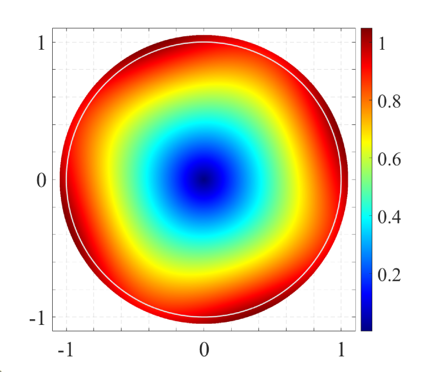
(b) $\|\boldsymbol{b}\|$ – copper

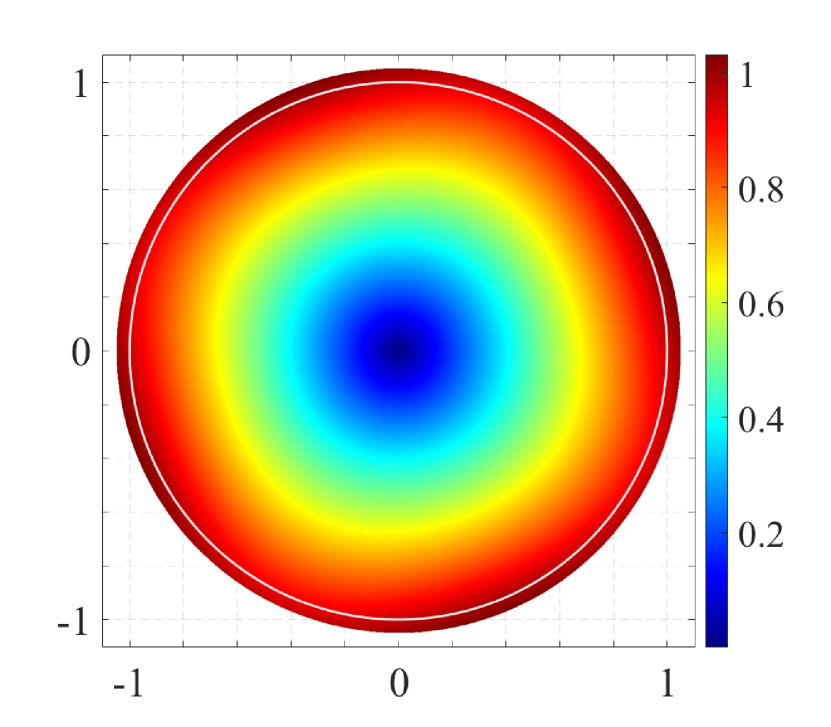
(c) $\|\boldsymbol{b}\|$ – aluminum

Figure 5: Magnetic field norm $\|\boldsymbol{b}\|$ (normalized by $\mu_{0}\kappa_{0}$), for different rotor materials in motors with $s=0.02,\;\zeta=0.05$.

Notice that for both the copper and aluminum rotors the maximum value of the magnetic field is two orders of magnitude less than in steel. One can also observe that the normalized magnetic field for aluminum and copper reaches its maximum value at the rotor boundary, given the absence of magnetization in these materials. The slightly larger extent for the maximum magnetic field zone for the copper rotor, is attributed to its higher electrical conductivity which results in higher induced currents than in aluminum.

4.3 Rotor temperature field

The full-field dimensionless temperature $(T-T_{a})/T_{a}\rightarrow T(r,\Theta)$ for the base case steel rotor is presented in Figure 6; the normalization with respect to the reference temperature $T^{a}$ adopted here as a more physically meaningful choice. Since the mean field dominates, the $\Theta$-dependent variations are completely masked by the scale used to plot Figure 6(a). The $\Theta$-dependent variation $\Re\left\{{\bar{T}}(r)\exp(-i2\Theta)\right\}$, whose amplitude is four orders of magnitude lower than the mean, is plotted by itself in Figure 6(b). According to the values given in Table 1 for the thermal characteristics of the idealized motor, the almost uniform temperature increase of the rotor is a mere $0.086^{\circ}C$ from an ambient airgap temperature of $20^{\circ}C$, with the maximum temperature occurring at the center.

(a) Full temperature field $T(r,\Theta)$

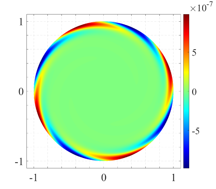
(b) $\Theta$-variation $\Re\left\{{\bar{T}}(r)\exp(-i2\Theta)\right\}$

Figure 6: Normalized temperature increase for the steel rotor (base case); (a) full field and (b) angular variation.

The influence of the rotor material on the dimensionless temperature increase $T(r,\Theta)$ in the base case motor is presented next in Figure 7. In comparing the results for steel in (a), copper in (b) and aluminum in (c), we notice that the temperature increase is almost uniform over the rotor, with the highest increase $0.086^{\circ}C$ occurring in steel, $0.062^{\circ}C$ for copper and $0.037^{\circ}C$ for aluminum.

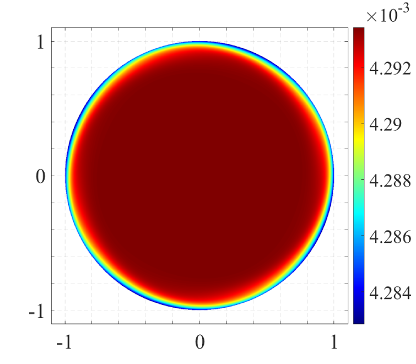
(a) $T(r,\Theta)$ – steel

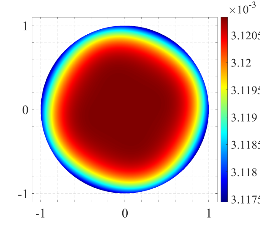
(b) $T(r,\Theta)$ – copper

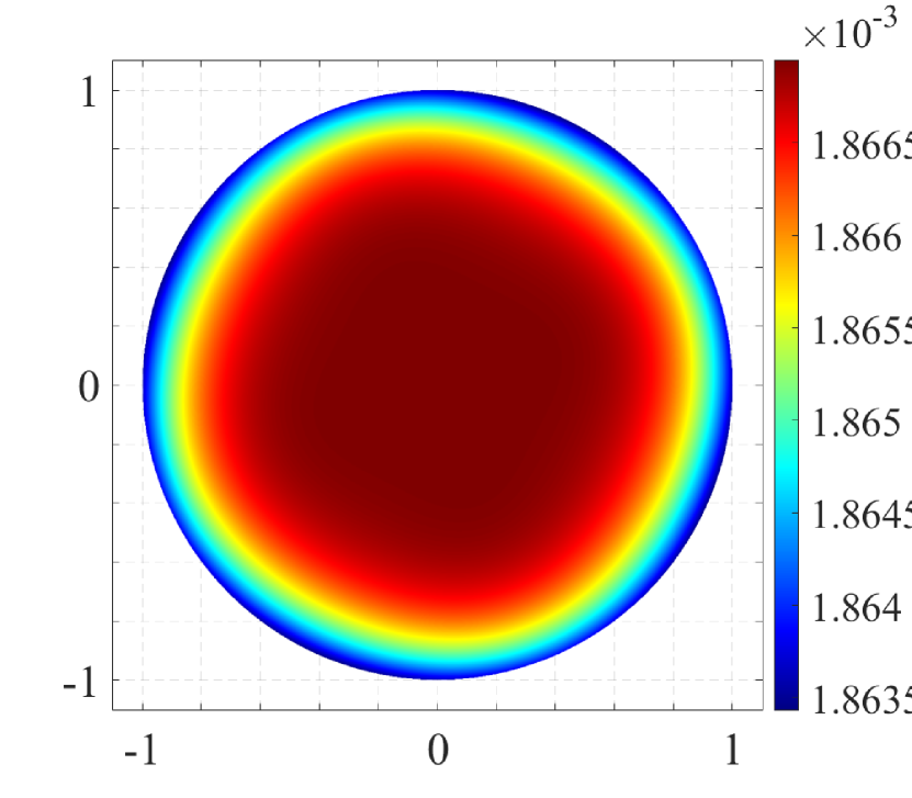
(c) $T(r,\Theta)$ – aluminum

Figure 7: Normalized temperature increase $T$ for the base case motor: (a) steel, (b) copper and (c) aluminum rotors.

Ohmic dissipation is the sole dissipation mechanism considered, as discussed in the first remark of Subsection 2.5 and depends on the relative frequency $\omega_{r}$. The relatively low frequency used (about $1Hz$, we consider $\omega_{r}$ at $2\%$ slip) explains the very low temperature increase found here.

4.4 Rotor current density, Lorentz and magnetic body forces

Current density The dimensionless current density field $j=j_{z}=-\gamma(\partial a/\partial t)$, (normalized by $\kappa_{0}/R_{1}$) for the base case motor is presented in Figure 8 for steel (a), copper (b) and aluminum (c) rotors, respectively. The currents for steel are forming thin plumes near the rotor surface because of the high magnetic permeability that concentrates the magnetic field at the rotor-airgap interface – see Figure 5(a) – limiting its penetration into the rotor. The current distribution for copper and aluminum rotors is very similar, given the absence of magnetization. Notice in Figure 8 that the maximum current values for steel are the lowest while the corresponding ones for copper are the highest, as expected by the different rotor material conductivities according to Table 1.

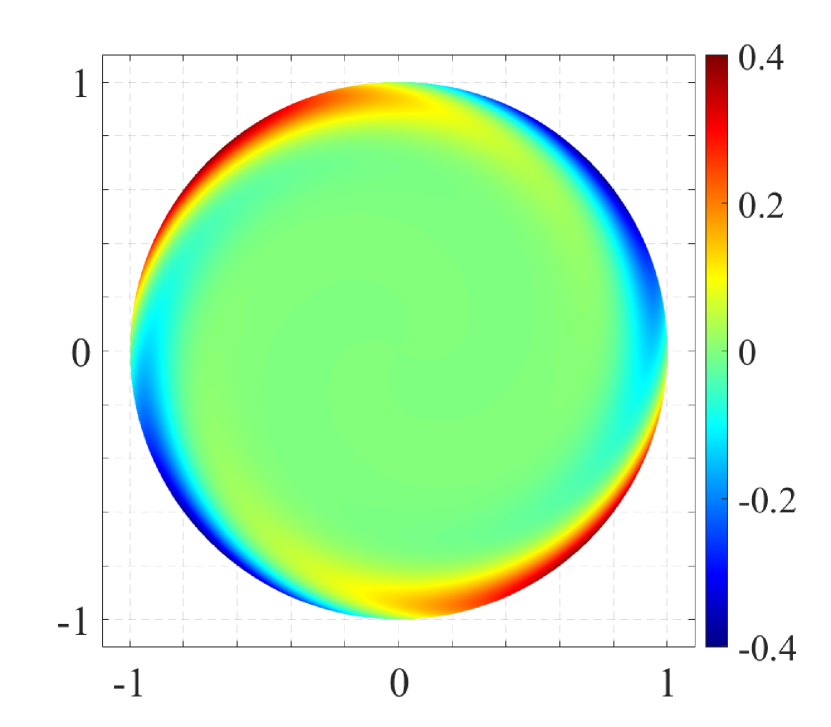
(a) $j(r,\Theta)$ - steel

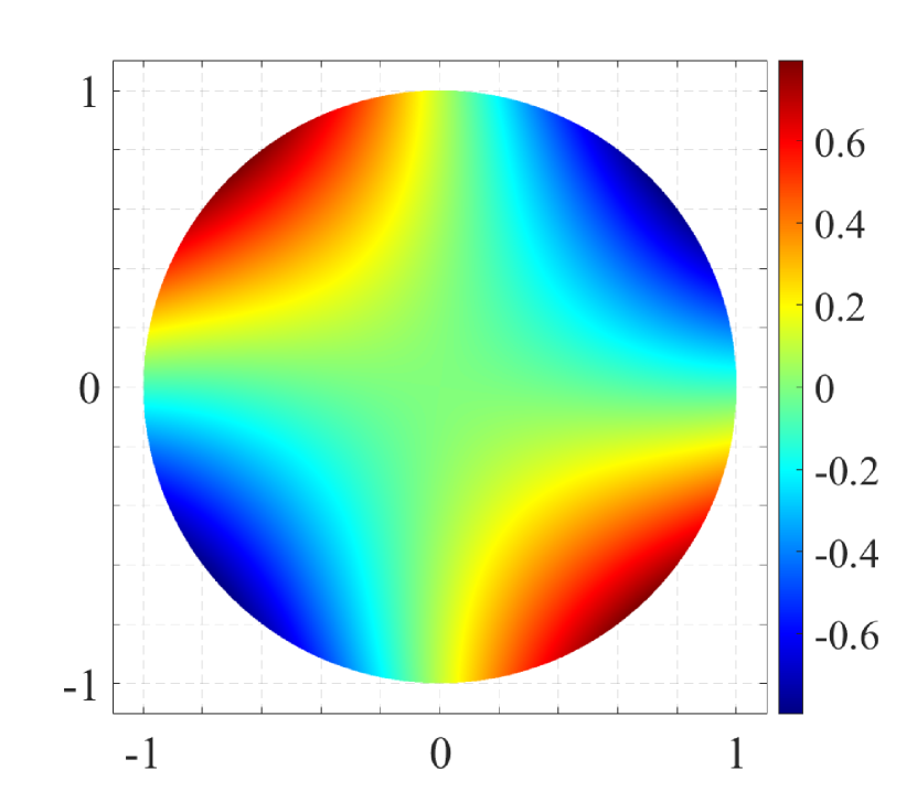
(b) $j(r,\Theta)$ - copper

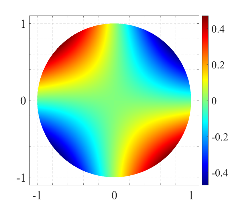
(c) $j(r,\Theta)$ - aluminum

Figure 8: Current density $j$ (normalized by $\kappa_{0}/R_{1}$), for the base case motor: (a) steel, (b) copper and (c) aluminum rotors.

Lorentz, magnetization and magnetostricive body forces The different components of the magnetic body force $\overset{m}{\boldsymbol{f}}$, defined as the divergence of the magnetic stress $\overset{m}{\boldsymbol{\sigma}}$ in (2.25), are

$$\overset{m}{\boldsymbol{f}}\equiv{\scriptstyle\boldsymbol{\nabla}}\!\boldsymbol{\cdot}\!\overset{m}{\boldsymbol{\sigma}}=\boldsymbol{j}\!\times\!\boldsymbol{b}+\boldsymbol{m}\!\boldsymbol{\cdot}\!(\boldsymbol{b}{\scriptstyle\boldsymbol{\nabla}})+\frac{\Lambda}{\mu}\boldsymbol{b}\!\boldsymbol{\cdot}\!({\scriptstyle\boldsymbol{\nabla}}\boldsymbol{b})\;;\quad\boldsymbol{m}=\frac{\chi}{\mu}\boldsymbol{b}\;,$$ (4.1)

where $\mu=\mu_{0}(1+\chi)$. The three different magnetic body force components in (4.1) are: the Lorentz body force: $\boldsymbol{j}\!\times\!\boldsymbol{b}$, a magnetization body force: $\boldsymbol{m}\!\boldsymbol{\cdot}\!(\boldsymbol{b}{\scriptstyle\boldsymbol{\nabla}})$ and a magnetostriction force: $(\Lambda/\mu)\boldsymbol{b}\!\boldsymbol{\cdot}\!({\scriptstyle\boldsymbol{\nabla}}\boldsymbol{b})$. The last two components are absent in non-magnetic copper and aluminum ($\chi\approx\Lambda\approx 0$).

Figure 9 shows the amplitude of the three different components of the electromagnetic force, (normalized by the amplitude of the centrifugal force density $\rho_{0}R_{1}\Omega^{2}$), for the base case motor with a steel rotor case. The first important observation is that the Lorentz forces are negligible, with their maximum value of the order of $1\%$ of the inertial forces. A straightforward dimensional analysis indicates $\|\boldsymbol{j}\|\approx\|\boldsymbol{b}\|/(\mu R_{1})$, giving $\|\boldsymbol{j}\!\times\!\boldsymbol{b}\|\approx\|\boldsymbol{b}\|^{2}/(\mu R_{1})$ for the Lorentz component of the body force, compared to the magnetic $\chi\|\boldsymbol{b}\|^{2}/(\mu R_{1})$ and magnetostrictive $\Lambda\|\boldsymbol{b}\|^{2}/(\mu R_{1})$ components.

(a) Lorentz $\|\boldsymbol{j}\!\times\!\boldsymbol{b}\|$

(b) Magnetization $\|\boldsymbol{m}\!\boldsymbol{\cdot}\!(\boldsymbol{b}{\scriptstyle\boldsymbol{\nabla}})\|$

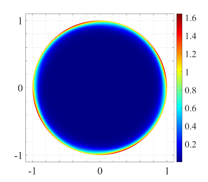
(c) Magnetostriction $\|(\Lambda/\mu)\boldsymbol{b}\!\boldsymbol{\cdot}\!({\scriptstyle\boldsymbol{\nabla}}\boldsymbol{b})\|$

Figure 9: Comparison of the different magnetic body forces (normalized by $\rho_{0}R_{1}\Omega^{2}$) for the base case motor with a steel rotor.

Observe that the magnetization force is larger than its inertial counterpart – up to approximately forty times at the rotor’s edge due to the highest magnetic field gradients there, according to Figure 5(b) – pointing to the importance of accounting for magnetization body forces in electric motor models. The magnetostrictive forces are not negligible and peak at about $160\%$ of their inertial counterpart (or about $5\%$ of the maximum magnetization forces), a somewhat surprising result in view of the same order $\chi$ and $\Lambda$ coefficients from Table 1 but explained by the different expressions for the corresponding forces in (4.1).

(a) $\|\overset{m}{\boldsymbol{f}}\|$ – steel

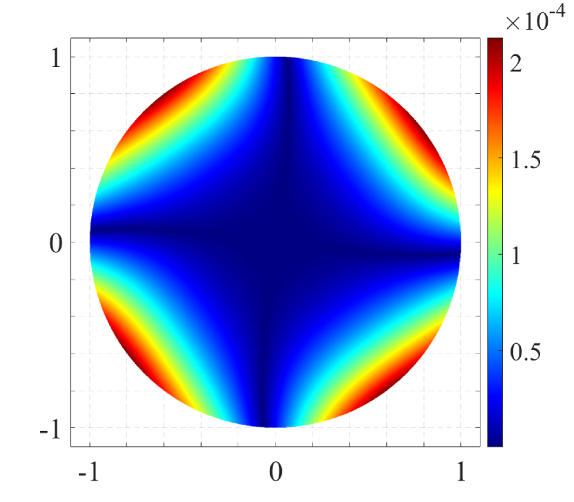
(b) $\|\overset{m}{\boldsymbol{f}}\|=\|\boldsymbol{j}\!\times\!\boldsymbol{b}\|$ – copper

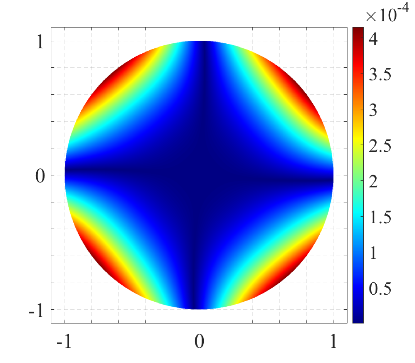
(c) $\|\overset{m}{\boldsymbol{f}}\|=\|\boldsymbol{j}\!\times\!\boldsymbol{b}\|$ – aluminum

Figure 10: Comparison of the total magnetic body force $\|\overset{m}{\boldsymbol{f}}\|$ (normalized by $\rho_{0}R_{1}\Omega^{2}$) for the base case motor with steel, copper and aluminum rotors. Notice that the magnetic body force is the Lorentz force $\boldsymbol{j}\!\times\!\boldsymbol{b}$ for the two non-magnetic materials.

The results in Figure 10 compare the magnetic body force (normalized by $\rho_{0}R_{1}\Omega^{2}$) of the base motor for the different rotor materials. Recall that the magnetic body force is just the Lorentz force for the copper and aluminum rotors, in view of their negligible magnetic properties. We emphasize again the orders of magnitude difference in the magnetic body force between the magnetic (steel) and the non-magnetic (copper, aluminum) materials. The Lorentz forces for the copper and aluminum rotor cases are comparable, given their close electric conductivity (see Table Table 1). Notice however that although the maximum current density is higher in the better conducting copper, the corresponding maximum Lorentz force is higher for the aluminum rotor.

4.5 Total and elastic stresses

In order to better assess the influence of the electromagnetic effects on the total $\boldsymbol{\sigma}$ and elastic $\overset{e}{\boldsymbol{\sigma}}$ stresses, we propose to compare them to the purely mechanical (only inertial body forces applied), plane strain elastic stress solution $\overset{i}{\boldsymbol{\sigma}}$ for the spinning rotor of the base case motor under angular velocity $\Omega$, a straightforward linear elasticity calculation resulting in the following stress field

$$\overset{i}{\sigma}_{rr}=\frac{\rho_{0}R_{1}^{2}\Omega^{2}}{8}\left(\frac{3-2\nu}{1-\nu}-\frac{3-2\nu}{1-\nu}r^{2}\right)\;,\quad\overset{i}{\sigma}_{r\theta}=0\;,\quad\overset{i}{\sigma}_{\theta\theta}=\frac{\rho_{0}R_{1}^{2}\Omega^{2}}{8}\left(\frac{3-2\nu}{1-\nu}-\frac{1+2\nu}{1-\nu}r^{2}\right)\;.$$ (4.2)

The maximum value for $\overset{i}{\sigma}_{rr}$ and $\overset{i}{\sigma}_{\theta\theta}$ is $[\rho_{0}(3-2\nu)/8(1-\nu)](R_{1}\Omega)^{2}$ and occurs at the rotor’s center $r=0$. For a more meaningful comparison to the purely mechanical stresses due to inertial effects, all future stress results are normalized by this maximum value, instead of $\rho_{0}(R_{1}\Omega)^{2}$ used thus far.

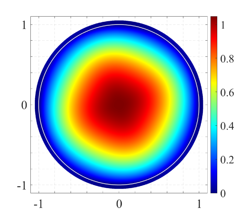
(a) $\sigma_{rr}(r,\Theta)$

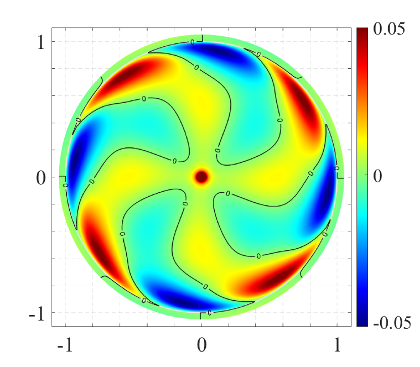
(b) $\sigma_{r\theta}(r,\Theta)$

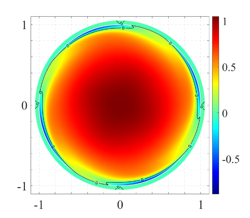
(c) $\sigma_{\theta\theta}(r,\Theta)$

Figure 11: Dimensionless total stresses in rotor and airgap (normalized by the maximum inertial stress): (a) normal, (b) shear and (c) hoop, for the base case steel motor.

The normalized total stress components for the base case motor with the steel rotor are presented in Figure 11, – with the stress fields shown both in the rotor and the airgap – where one can see the continuity of the normal $\sigma_{rr}$ and shear $\sigma_{r\theta}$ components at the rotor-airgap interface.

The total normal stress $\sigma_{rr}$ is always positive, never exceeding the maximum, purely inertial value, as seen in Figure 11(a). It monotonically increases away from the rotor’s edge and reaches its maximum at the center, region where the electromagnetic effects are negligible, in contrast to the rotor’s edge. The total shear stress $\sigma_{r\theta}$ varies symmetrically between approximately $\pm 5\%$ of the maximum (normal) inertial stress, following the angular pattern imposed by the $\cos(2\Theta)$ and $\sin(2\Theta)$ terms. Also notice in Figure 11(b) the singularity in $r=0$ – truncated in the figure – due to the external torque applied there. The total hoop stress $\sigma_{\theta\theta}$ is positive in most of the central domain, where inertial effects dominate, with the same maximum value as for the purely inertial case. The influence of the magnetic field is however evident on the rotor’s edge, where a compressive stress of the same absolute value as the maximum inertial stress does appear.

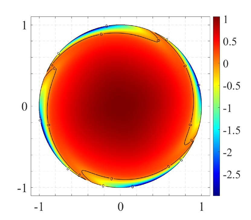
(a) $\overset{e}{\sigma}_{rr}(r,\Theta)$

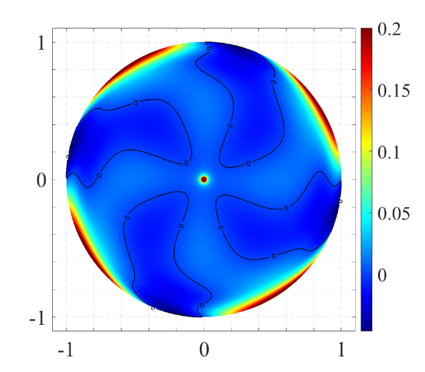
(b) $\overset{e}{\sigma}_{r\theta}(r,\Theta)$

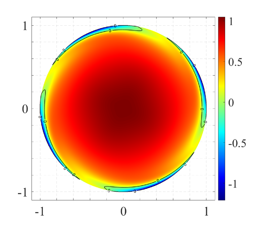
(c) $\overset{e}{\sigma}_{\theta\theta}(r,\Theta)$

Figure 12: Dimensionless elastic stresses in rotor (normalized by the maximum inertial stress): (a) normal, (b) shear and (c) hoop, for the base case steel motor.

The normalized elastic stress $\overset{e}{\boldsymbol{\sigma}}$ components in the rotor are given in Figure 12 and differ significantly from their total stress counterparts $\boldsymbol{\sigma}$, as a simple comparison between Figure 11 and Figure 12 shows. The elastic stress components are approximately their inertial counterparts $\overset{i}{\boldsymbol{\sigma}}$, given by (4.2), due to the weak magnetic fields at the center of the rotor. However, due to the strong magnetic fields at the rotor boundary, boundary layers develop near its edge resulting in strong compressive components, up to $250\%$ times for the normal and $125\%$ for the hoop components respectively, higher than the corresponding maximal inertial stress. For the shear stress component, a comparison between Figure 11(b) and Figure 12(b) shows larger elastic shear stresses, in particular near the rotor’s edge, due to the mechanical torque produced.

4.6 Rotor torque

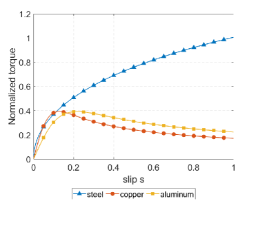
Figure 13: Dimensionless torque $\mathcal{T}$ (normalized by $\pi\rho_{0}R_{1}^{4}\Omega^{2}s_{0}$) vs slip coefficient $s=\omega_{r}/\omega$ for the base case motor with three different rotor materials.

The torque $\mathcal{T}$, normalized by $\pi\rho_{0}R_{1}^{4}\Omega^{2}s_{0}$, is plotted in Figure 13 as a function of the slip coefficient $s$. For low $\kappa_{0}$ values (where the magnetic field remains below the saturation level for steel for all slip values considered) the steel rotor shows higher torque than its copper and aluminum counterparts across almost all the slip range, only slightly dominated by the copper rotor in a region around $5-10\%$ slip.

For high $\kappa_{0}$ values, the monotonic increase of the torque as a function of slip for steel – due to its linear magnetic response – is misleading, as saturation may occur, which is not accounted for in the model. In the base case motor, the magnetic field for the steel rotor is already close to saturation for $\kappa_{0}=1.3\!\times\!10^{4},s=2\%$ with a value of $1.3$T (see Figure 2(a)). In this case, it is expected that due to magnetic saturation, the steel torque-slip curve above $s=2\%$ should be reaching a maximum torque, as is the case for the copper and aluminum rotors. For $s=5\%$ or higher, the copper motor would produce a larger torque than its steel counterpart.

5 Conclusion

Using the direct approach of continuum mechanics, based on Kovetz (2000), a general framework that couples the electromagnetic, thermal and mechanical effects is derived and subsequently applied to formulate the boundary value problem for electric motors. Particular attention is paid to the derivation of the coupled constitutive equations for isotropic materials under small strain but arbitrary magnetization. As a first application, the theory is employed for the analytical modeling of an idealized asynchronous motor for which we calculate the magnetic, thermal, stress fields and its torque. To better assess the influence of magnetization on stresses, three different rotor materials are examined: electric steel, copper and aluminum and different airgap and slip parameters are considered using realistic geometric and operational regime values (see Lubin et al. (2011)) and material parameters (see Aydin et al. (2017)). Given the linearized magnetic constitutive model adopted for the sake of an analytical solution, the applied current amplitude is chosen to produce magnetic fields below saturation levels.

Magnetic field results show, as expected, the presence of a boundary layer at the rotor’s edge for the steel case and more diffuse patterns for the non-magnetic materials; about two order of magnitude difference is observed in the maximum magnetic field between the magnetic and non-magnetic materials. Comparing the Lorentz, magnetization and the magnetostrictive forces in the steel rotor case we find that the first are negligible (more than three orders of magnitude less for the first compared to the last two). Moreover, magnetostrictive body forces – resulting from the constitutive coupling between stress and magnetization effects – although smaller that their magnetic counterparts, are considerably higher than the Lorentz. This is an important finding of our calculations, since the former are usually neglected in the electric motor calculations available in the literature. As expected the magnetic body forces found in the steel rotor are concentrated along a boundary layer and significantly higher than their counterparts for the non-magnetic materials that are more diffusely distributed, thus explaining the importance of magnetic rotors for the production of a much higher torque for a given current amplitude, as long as the magnetic field remains below saturation levels.

Due to the realistic thermal parameters used in the calculations, the temperature increase in the rotor is negligible with the temperature maximum appearing in the rotor’s center. Significant differences are found in the current density distribution between the magnetic and non-magnetic materials, with a boundary layer appearing in the first and diffuse patterns in the second case.

The analytical solution of the model allows the comparison of the different parts of the stress tensor (elastic and total) to the purely mechanical stresses due to inertia, revealing the significant influence of electromagnetic phenomena on the resulting stress state. Although the maximum value of total stress’ normal components never exceed their purely inertial counterparts, the corresponding elastic stress components do so by developing a stress concentration boundary layer where compressive radial and hoop stresses can be up to three times higher than the maximum inertial value. Moreover, elastic shear stresses are considerably higher than the total stress and concentrated on a boundary layer about the rotor’s edge.

In spite of its limitations, the proposed analytical model shows clearly the importance of correctly accounting for the coupled magneto-mechanical effects for the accurate calculation of the stress fields. The proposed methodology for solving general boundary value problems is applicable to more complicated motor geometries and nonlinear constitutive responses that include moderate strains, magnetic saturation and dissipative effects. For these problems, a numerical approach based on coupled variational principles is necessary (e.g. see Thomas and Triantafyllidis (2009)) as well as special numerical techniques for the time-dependent aspects of the problem; further research is planned in this direction.

ACKNOWLEDGMENTS

The work of N. H. is supported by a Fellowship from the André Citroën Chair of the Ecole Polytechnique.

6 References

Appendix A Isotropic, small strain, arbitrary magnetization constitutive laws

The derivation of the constitutive laws for an isotropic magnetoelastic material for small strain $\boldsymbol{\epsilon}$, but arbitrary magnetic field $\boldsymbol{b}$, although straightforward requires lengthy calculations. Although such calculations have been presented in the literature a long time ago by Pao and Yeh (1973), following the early works on magnetoelasticity by Brown (1966), a direct comparison with our results is not possible due to the different formulations adopted (e.g. different independent variables of the free energy densities, different definitions of total stress etc.). Moreover, such derivations are not always done consistently in the available literature; a linearized version of the invariants is often considered, thus violating the objective nature of the free energy since the small strain tensor $\boldsymbol{\epsilon}$ is not objective.

Derivations are presented here for two different scenarios: the first assumes the most general form of Helmholtz free energy $\hat{\psi}(I_{k},J_{k},T)$ and the second is based on the decoupled form $\hat{\psi}=\hat{\psi}_{e}(I_{k})+\hat{\psi}_{m}(J_{k})+\hat{\psi}_{th}(T)$ proposed in (2.23). In both cases terms in $\boldsymbol{\epsilon}\;\boldsymbol{b}$ are kept, providing a more general result than the one presented in (2.25).

i) General form of free energy $\psi=\hat{\psi}(I_{1},I_{2},I_{3},J_{1},J_{2},J_{3},T)$ Recall that the current configuration expressions for the magnetization and total stress in (2.21) are found by differentiating the Helmoltz free energy $\hat{\psi}(\boldsymbol{C},\boldsymbol{B},T)$. In the case of an isotropic material $\hat{\psi}(\boldsymbol{C},\boldsymbol{B},T)=\hat{\psi}(I_{1},I_{2},I_{3},J_{1},J_{2},J_{3},T)$ whose invariants are expressed in terms of the right Cauchy-Green tensor $\boldsymbol{C}\equiv\boldsymbol{F}^{T}\!\boldsymbol{\cdot}\!\boldsymbol{F}$ and $\boldsymbol{B}\equiv\boldsymbol{b}\!\boldsymbol{\cdot}\!\boldsymbol{F}$ according to (2.23).

Applying the chain rule of differentiation to the expressions in (2.21), one obtains

$$\begin{array}[]{rl}\boldsymbol{m}\!\!\!&=\displaystyle-2{\rho_{0}\over\sqrt{I_{3}}}\left(\frac{\partial\hat{\psi}}{\partial J_{1}}\boldsymbol{I}+\frac{\partial\hat{\psi}}{\partial J_{2}}\boldsymbol{c}+\frac{\partial\hat{\psi}}{\partial J_{3}}\boldsymbol{c}^{2}\right)\!\boldsymbol{\cdot}\!\boldsymbol{b}\;,\vspace{0.2cm}\\ \boldsymbol{\sigma}\!\!\!&=\displaystyle 2{\rho_{0}\over\sqrt{I_{3}}}\bigg{[}\frac{\partial\hat{\psi}}{\partial I_{1}}\boldsymbol{c}+\frac{\partial\hat{\psi}}{\partial I_{2}}(\text{tr}({\boldsymbol{c}})\boldsymbol{c}-\boldsymbol{c}^{2})+\frac{\partial\hat{\psi}}{\partial I_{3}}\text{det}({\boldsymbol{c}})\boldsymbol{I}-\frac{\partial\hat{\psi}}{\partial J_{1}}\boldsymbol{b}\boldsymbol{b}+\frac{\partial\hat{\psi}}{\partial J_{3}}(\boldsymbol{c}\!\boldsymbol{\cdot}\!\boldsymbol{b})(\boldsymbol{c}\!\boldsymbol{\cdot}\!\boldsymbol{b})\bigg{]}+\vspace{0.2cm}\\ &+\displaystyle\frac{1}{\mu_{0}}\Big{(}\boldsymbol{b}\boldsymbol{b}-\frac{1}{2}(\boldsymbol{b}\!\boldsymbol{\cdot}\!\boldsymbol{b})\boldsymbol{I}\Big{)}-\Big{(}\boldsymbol{m}\boldsymbol{b}+\boldsymbol{b}\boldsymbol{m}-(\boldsymbol{b}\!\boldsymbol{\cdot}\!\boldsymbol{m})\boldsymbol{I}\Big{)}\;,\end{array}$$ (A.1)

where the left Cauchy-Green tensor $\boldsymbol{c}\equiv\boldsymbol{F}\!\boldsymbol{\cdot}\!\boldsymbol{F}^{T}$ appears naturally in the constitutive relations (A.1). The subsequent algebra of small strain linearization is considerably simplified by noting that the invariants involved can be alternatively expressed in terms of $\boldsymbol{c}$ and $\boldsymbol{b}$ as follows

$$\begin{array}[]{l}I_{1}=\displaystyle\text{tr}({\boldsymbol{c}}),\quad I_{2}=\frac{1}{2}(\text{tr}({\boldsymbol{c}})^{2}-\text{tr}({\boldsymbol{c}\!\boldsymbol{\cdot}\!\boldsymbol{c}})),\quad I_{3}=\text{det}({\boldsymbol{c}})\;;\quad\boldsymbol{c}\equiv\boldsymbol{F}\!\boldsymbol{\cdot}\!\boldsymbol{F}^{T}\;,\vspace{0.2cm}\\ J_{1}=\displaystyle\boldsymbol{b}\!\boldsymbol{\cdot}\!\boldsymbol{b}=\|\boldsymbol{b}\|^{2},\quad J_{2}=\boldsymbol{b}\!\boldsymbol{\cdot}\!\boldsymbol{c}\!\boldsymbol{\cdot}\!\boldsymbol{b},\quad J_{3}=\boldsymbol{b}\!\boldsymbol{\cdot}\!\boldsymbol{c}^{2}\!\boldsymbol{\cdot}\!\boldsymbol{b}\;.\end{array}$$ (A.2)

Expanding the expressions in (A.1) about $\boldsymbol{c}=\boldsymbol{I}$ up to the first order in the small strain tensor $\boldsymbol{\epsilon}~{}\equiv~{}(1/2)({\scriptstyle\boldsymbol{\nabla}}\boldsymbol{u}+\boldsymbol{u}{\scriptstyle\boldsymbol{\nabla}})$, for $\|\boldsymbol{\epsilon}\|\ll 1$, we obtain up to $O(\|\boldsymbol{\epsilon}\|^{2})$

$$\boldsymbol{m}\approx\displaystyle\boldsymbol{m}(\boldsymbol{c}=\boldsymbol{I},\boldsymbol{b},T)+\frac{\partial\boldsymbol{m}}{\partial\boldsymbol{c}}\Big{|}_{\boldsymbol{c}=\boldsymbol{I}}\boldsymbol{:}2\boldsymbol{\epsilon},\quad\boldsymbol{\sigma}\approx\boldsymbol{\sigma}(\boldsymbol{c}=\boldsymbol{I},\boldsymbol{b},T)+\frac{\partial\boldsymbol{\sigma}}{\partial\boldsymbol{c}}\Big{|}_{\boldsymbol{c}=\boldsymbol{I}}\boldsymbol{:}2\boldsymbol{\epsilon}\;;\quad\boldsymbol{c}-\boldsymbol{I}\approx 2\boldsymbol{\epsilon}\;.$$ (A.3)

After lengthy algebraic manipulations of (A.1) and (A.3), the following expression for the magnetization $\boldsymbol{m}$ is found involving the scalar quantities $\zeta_{i}(\|\boldsymbol{b}\|)\;,i=1,\cdots,4$

$$\begin{array}[]{rl}\boldsymbol{m}\!\!\!&=\displaystyle\zeta_{1}\boldsymbol{b}+\zeta_{2}\text{tr}({\boldsymbol{\epsilon}})\boldsymbol{b}+\zeta_{3}(\boldsymbol{b}\!\boldsymbol{\cdot}\!\boldsymbol{\epsilon}\!\boldsymbol{\cdot}\!\boldsymbol{b})\boldsymbol{b}+\zeta_{4}\boldsymbol{\epsilon}\!\boldsymbol{\cdot}\!\boldsymbol{b}\;;\vspace{0.2cm}\\ \zeta_{1}(\|\boldsymbol{b}\|)\!\!\!&\equiv\displaystyle-2\rho_{0}\left[\frac{\partial\hat{\psi}}{\partial J_{1}}+\frac{\partial\hat{\psi}}{\partial J_{2}}+\frac{\partial\hat{\psi}}{\partial J_{3}}\right]_{\boldsymbol{c}=\boldsymbol{I}}\;,\vspace{0.2cm}\\ \zeta_{2}(\|\boldsymbol{b}\|)\!\!\!&\equiv\displaystyle-\zeta_{1}(\|\boldsymbol{b}\|)-4\rho_{0}\left[\frac{\partial}{\partial I_{1}}+2\frac{\partial}{\partial I_{2}}+\frac{\partial}{\partial I_{3}}\right]\left[\frac{\partial\hat{\psi}}{\partial J_{1}}+\frac{\partial\hat{\psi}}{\partial J_{2}}+\frac{\partial\hat{\psi}}{\partial J_{3}}\right]_{\boldsymbol{c}=\boldsymbol{I}}\;,\vspace{0.2cm}\\ \zeta_{3}(\|\boldsymbol{b}\|)\!\!\!&\equiv\displaystyle-4\rho_{0}\left[\frac{\partial}{\partial J_{2}}+2\frac{\partial}{\partial J_{3}}\right]\left[\frac{\partial\hat{\psi}}{\partial J_{1}}+\frac{\partial\hat{\psi}}{\partial J_{2}}+\frac{\partial\hat{\psi}}{\partial J_{3}}\right]_{\boldsymbol{c}=\boldsymbol{I}}\;,\vspace{0.2cm}\\ \zeta_{4}(\|\boldsymbol{b}\|)\!\!\!&\equiv\displaystyle-4\rho_{0}\left[\frac{\partial\hat{\psi}}{\partial J_{2}}+2\frac{\partial\hat{\psi}}{\partial J_{3}}\right]_{\boldsymbol{c}=\boldsymbol{I}}\;.\end{array}$$ (A.4)

The corresponding small strain linearization expressions yield a total stress $\boldsymbol{\sigma}$ as the sum of an elastic $\overset{e}{\boldsymbol{\sigma}}$, a magnetic $\overset{m}{\boldsymbol{\sigma}}$ and a magnetostrictive $\overset{ms}{\boldsymbol{\sigma}}$ (involving terms of the order $\boldsymbol{\epsilon}\;\boldsymbol{b}$) component

$$\begin{array}[]{rl}\boldsymbol{\sigma}\!\!\!&=\displaystyle\overset{e}{\boldsymbol{\sigma}}+\overset{m}{\boldsymbol{\sigma}}+\overset{ms}{\boldsymbol{\sigma}}\;;\vspace{0.2cm}\\ \overset{e}{\boldsymbol{\sigma}}\!\!\!&\equiv\displaystyle\lambda\text{tr}({\boldsymbol{\epsilon}})\boldsymbol{I}+2G\boldsymbol{\epsilon}\;,\vspace{0.2cm}\\ \overset{m}{\boldsymbol{\sigma}}\!\!\!&\equiv\displaystyle\frac{1}{\mu_{0}}\left[\boldsymbol{b}\boldsymbol{b}-\frac{1}{2}(\boldsymbol{b}\!\boldsymbol{\cdot}\!\boldsymbol{b})\boldsymbol{I}\right]-\zeta_{1}\left[\boldsymbol{b}\boldsymbol{b}-(\boldsymbol{b}\!\boldsymbol{\cdot}\!\boldsymbol{b})\boldsymbol{I}\right]-\frac{\zeta_{4}}{2}\boldsymbol{b}\boldsymbol{b}\;,\vspace{0.2cm}\\ \overset{ms}{\boldsymbol{\sigma}}\!\!\!&\equiv\displaystyle\Sigma_{0}\boldsymbol{I}+[\Sigma_{1}\boldsymbol{b}\boldsymbol{b}+\zeta_{2}(\boldsymbol{b}\!\boldsymbol{\cdot}\!\boldsymbol{b})\boldsymbol{I}]\text{tr}({\boldsymbol{\epsilon}})+[\Sigma_{2}\boldsymbol{I}+\Sigma_{4}\boldsymbol{b}\boldsymbol{b}+\zeta_{3}(\boldsymbol{b}\!\boldsymbol{\cdot}\!\boldsymbol{b})\boldsymbol{I}](\boldsymbol{b}\!\boldsymbol{\cdot}\!\boldsymbol{\epsilon}\!\boldsymbol{\cdot}\!\boldsymbol{b})+\Sigma_{3}[(\boldsymbol{b}\!\boldsymbol{\cdot}\!\boldsymbol{\epsilon})\boldsymbol{b}+\boldsymbol{b}(\boldsymbol{\epsilon}\!\boldsymbol{\cdot}\!\boldsymbol{b})]\;,\vspace{0.2cm}\\ \lambda(\|\boldsymbol{b}\|)\!\!\!&\equiv\displaystyle 2\rho_{0}\left[\frac{\partial\hat{\psi}}{\partial I_{3}}-\frac{\partial\hat{\psi}}{\partial I_{1}}\right]_{\boldsymbol{c}=\boldsymbol{I}}+4\rho_{0}\left[\left(\frac{\partial}{\partial I_{1}}+2\frac{\partial}{\partial I_{2}}+\frac{\partial}{\partial I_{3}}\right)\left(\frac{\partial\hat{\psi}}{\partial I_{1}}+2\frac{\partial\hat{\psi}}{\partial I_{2}}+\frac{\partial\hat{\psi}}{\partial I_{3}}\right)\right]_{\boldsymbol{c}=\boldsymbol{I}}\;,\vspace{0.2cm}\\ G(\|\boldsymbol{b}\|)\!\!\!&=\displaystyle 2\rho_{0}\left[\frac{\partial\hat{\psi}}{\partial I_{1}}+\frac{\partial\hat{\psi}}{\partial I_{2}}\right]_{\boldsymbol{c}=\boldsymbol{I}}\;,\vspace{0.2cm}\\ \Sigma_{0}(\|\boldsymbol{b}\|)\!\!\!&\equiv\displaystyle 2\rho_{0}\left[\frac{\partial\hat{\psi}}{\partial I_{1}}+2\frac{\partial\hat{\psi}}{\partial I_{2}}+\frac{\partial\hat{\psi}}{\partial I_{3}}\right]_{\boldsymbol{c}=\boldsymbol{I}}\;,\vspace{0.2cm}\\ \Sigma_{1}(\|\boldsymbol{b}\|)\!\!\!&\equiv\displaystyle-\zeta_{2}(\|\boldsymbol{b}\|)-\frac{1}{2}\zeta_{4}(\|\boldsymbol{b}\|)+\Sigma_{2}(\|\boldsymbol{b}\|)\;,\vspace{0.2cm}\\ \Sigma_{2}(\|\boldsymbol{b}\|)\!\!\!&=\displaystyle\zeta_{4}(\|\boldsymbol{b}\|)+4\rho_{0}\left[\left(\frac{\partial}{\partial J_{2}}+2\frac{\partial}{\partial J_{3}}\right)\left(\frac{\partial\hat{\psi}}{\partial I_{1}}+2\frac{\partial\hat{\psi}}{\partial I_{2}}+\frac{\partial\hat{\psi}}{\partial I_{3}}\right)\right]_{\boldsymbol{c}=\boldsymbol{I}}\;,\vspace{0.2cm}\\ \Sigma_{3}(\|\boldsymbol{b}\|)\!\!\!&\equiv\displaystyle-\zeta_{4}(\|\boldsymbol{b}\|)+4\rho_{0}\left[\frac{\partial\hat{\psi}}{\partial J_{3}}\right]_{\boldsymbol{c}=\boldsymbol{I}}\;,\vspace{0.2cm}\\ \Sigma_{4}(\|\boldsymbol{b}\|)\!\!\!&\equiv\displaystyle-\zeta_{3}(\|\boldsymbol{b}\|)+4\rho_{0}\left[\left(\frac{\partial}{\partial J_{2}}+2\frac{\partial}{\partial J_{3}}\right)\left(\frac{\partial\hat{\psi}}{\partial J_{2}}+2\frac{\partial\hat{\psi}}{\partial J_{3}}\right)\right]_{\boldsymbol{c}=\boldsymbol{I}}\;,\end{array}$$ (A.5)

and are expressed in terms of seven magnetic field-dependent coefficients: the two Lamé coefficients $\lambda(\|\boldsymbol{b}\|)$ and $G(\|\boldsymbol{b}\|)$ plus five more scalars $\Sigma_{i}(\|\boldsymbol{b}\|)\;,i=0,\cdots,4$. This expansion proves that in a first order approximation in $\boldsymbol{\epsilon}$, the coefficients in the expressions for $\boldsymbol{m}$ and $\boldsymbol{\sigma}$ depend solely on $||\boldsymbol{b}||$. The fact that $\lambda$ and $G$ – and hence the Young’s modulus $E$ – may depend on $||\boldsymbol{b}||$ is referred to as the $\Delta E$ effect (see e.g. Daniel and Hubert (2009)).

ii) Decoupled form of the free energy $\psi=\hat{\psi}_{e}(I_{1},I_{2},I_{3})+\hat{\psi}_{m}(,J_{1},J_{2},J_{3})+\hat{\psi}_{th}(T)$ Under the additional hypothesis of additive decomposition for the specific free energy in (2.23), one obtains the simplification $\zeta_{2}=-\zeta_{1}$ yielding from (A.4) the following expression for the magnetization $\boldsymbol{m}$

$$\begin{array}[]{rl}\boldsymbol{m}\!\!\!&=\zeta_{1}[1-\text{tr}({\boldsymbol{\epsilon}})]\boldsymbol{b}+\zeta_{3}(\boldsymbol{b}\!\boldsymbol{\cdot}\!\boldsymbol{\epsilon}\!\boldsymbol{\cdot}\!\boldsymbol{b})\boldsymbol{b}+\zeta_{4}\boldsymbol{\epsilon}\!\boldsymbol{\cdot}\!\boldsymbol{b}\;,\vspace{0.2cm}\\ \zeta_{1}(\|\boldsymbol{b}\|)\!\!\!&=\displaystyle-2\rho_{0}\left[\frac{\partial\hat{\psi}_{m}}{\partial J_{1}}+\frac{\partial\hat{\psi}_{m}}{\partial J_{2}}+\frac{\partial\hat{\psi}_{m}}{\partial J_{3}}\right]_{\boldsymbol{c}=\boldsymbol{I}}\;,\vspace{0.2cm}\\ \zeta_{3}(\|\boldsymbol{b}\|)\!\!\!&=\displaystyle-4\rho_{0}\left[\frac{\partial}{\partial J_{2}}+2\frac{\partial}{\partial J_{3}}\right]\left[\frac{\partial\hat{\psi}_{m}}{\partial J_{1}}+\frac{\partial\hat{\psi}_{m}}{\partial J_{2}}+\frac{\partial\hat{\psi}_{m}}{\partial J_{3}}\right]_{\boldsymbol{c}=\boldsymbol{I}}\;,\vspace{0.2cm}\\ \zeta_{4}(\|\boldsymbol{b}\|)\!\!\!&=\displaystyle-4\rho_{0}\left[\frac{\partial\hat{\psi}_{m}}{\partial J_{2}}+2\frac{\partial\hat{\psi}_{m}}{\partial J_{3}}\right]_{\boldsymbol{c}=\boldsymbol{I}}\;.\end{array}$$ (A.6)

The corresponding expressions for the elastic $\overset{e}{\boldsymbol{\sigma}}$, magnetic $\overset{m}{\boldsymbol{\sigma}}$ and magnetostrictive $\overset{ms}{\boldsymbol{\sigma}}$ components of the total stress $\boldsymbol{\sigma}$ simplify from their corresponding counterparts in (A.5) into

$$\begin{array}[]{rl}\overset{e}{\boldsymbol{\sigma}}\!\!\!&=\displaystyle\lambda\text{tr}({\boldsymbol{\epsilon}})\boldsymbol{I}+2G\boldsymbol{\epsilon}\;,\vspace{0.2cm}\\ \overset{m}{\boldsymbol{\sigma}}\!\!\!&=\displaystyle\frac{1}{\mu_{0}}\left[\boldsymbol{b}\boldsymbol{b}-\frac{1}{2}(\boldsymbol{b}\!\boldsymbol{\cdot}\!\boldsymbol{b})\boldsymbol{I}\right]-\zeta_{1}\left[\boldsymbol{b}\boldsymbol{b}-(\boldsymbol{b}\!\boldsymbol{\cdot}\!\boldsymbol{b})\boldsymbol{I}\right]-\frac{\zeta_{4}}{2}\boldsymbol{b}\boldsymbol{b}\;,\vspace{0.2cm}\\ \overset{ms}{\boldsymbol{\sigma}}\!\!\!&=\displaystyle[\Sigma_{4}\boldsymbol{b}\boldsymbol{b}+\zeta_{3}(\boldsymbol{b}\!\boldsymbol{\cdot}\!\boldsymbol{b})\boldsymbol{I}](\boldsymbol{b}\!\boldsymbol{\cdot}\!\boldsymbol{\epsilon}\!\boldsymbol{\cdot}\!\boldsymbol{b})+\Sigma_{3}\left[(\boldsymbol{b}\!\boldsymbol{\cdot}\!\boldsymbol{\epsilon})\boldsymbol{b}+\boldsymbol{b}(\boldsymbol{\epsilon}\!\boldsymbol{\cdot}\!\boldsymbol{b})\right)]\;,\end{array}$$ (A.7)

where the scalars $\zeta_{1}$, $\zeta_{3}$, $\zeta_{4}$ are given in (A.6) and $\Sigma_{3}$ and $\Sigma_{4}$ given in (A.5) but with $\hat{\psi}$ replaced by $\psi_{m}$. In deriving (A.7) from (A.5) under the decoupling hypothesis, the pre-stress $\Sigma_{0}$ and the corresponding Lamé coefficients $\lambda,G$ are now constants independent of the magnetic field $\boldsymbol{b}$. It is further assumed that the elastic prestress $\Sigma_{0}=0$. Five functions of $\|\boldsymbol{b}\|$ are thus need to characterize the response of an isotropic, small strain, decoupled-energy, magnetoelastic material: $\zeta_{1},\zeta_{3},\zeta_{4},\Sigma_{3},\Sigma_{4}$.

A final remark is in order here to connect the above results to the constitutive equation in (2.25) that neglects the magnetostrictive stress component $\overset{ms}{\boldsymbol{\sigma}}$. The reason for this simplification is that for small strains ($\|\boldsymbol{\epsilon}\|\ll 1$) and assuming that the constants appearing in $\overset{m}{\boldsymbol{\sigma}}$ and $\overset{ms}{\boldsymbol{\sigma}}$ are of the same order of magnitude, one deduces that $\|\overset{ms}{\boldsymbol{\sigma}}\|\ll\|\overset{m}{\boldsymbol{\sigma}}\|$. In the field of dielectric elastomers – a completely analogous problem where $\boldsymbol{e}\rightarrow\boldsymbol{b},\ \boldsymbol{p}\rightarrow\boldsymbol{m},\ \varepsilon_{0}\rightarrow\mu_{0}^{-1}$ – similar results that neglect the coupled terms are justified under the typical hypothesis of small strain and moderate electric field: $\boldsymbol{\epsilon}=O(\zeta)$, $\boldsymbol{e}=O(\sqrt{\zeta})$, where $\zeta$ a vanishingly small parameter (e.g. see Tian et al. (2012); Lefevre and Lopez-Pamies (2017)). The two coefficients $\zeta_{1}$ and $\zeta_{4}$ needed for the determination of $\overset{m}{\boldsymbol{\sigma}}$ are related to the magnetic susceptibility $\chi(\|\boldsymbol{b}\|)$ and magnetostrictive coefficient $\Lambda(\|\boldsymbol{b}\|)$ by: $\zeta_{1}(\|\boldsymbol{b}\|)=\chi(\|\boldsymbol{b}\|)/[\mu_{0}(1+\chi(\|\boldsymbol{b}\|))]$ and $\zeta_{4}(\|\boldsymbol{b}\|)=-2\Lambda(\|\boldsymbol{b}\|)/[\mu_{0}(1+\chi(\|\boldsymbol{b}\|))]$.

Appendix B Particular and homogeneous solution elastic stress fields

From (3.25) and (3.26), the particular solution stress field $\overset{e}{\boldsymbol{\sigma}}^{{}_{V}}$ components are

$$\begin{array}[]{rl}\overset{e}{\sigma}^{{}_{V}}_{rr}=&\displaystyle\!\!\!V-\frac{1}{2}{{1-2\nu}\over{1-\nu}}\left(\frac{2}{r^{2}}\int_{0}^{r}rV_{0}\mathrm{d}r+(2p-1)r^{{}^{2p-2}}\int_{0}^{r}\frac{V_{cs}}{r^{2p-1}}\mathrm{d}r-\frac{2p+1}{r^{2p+2}}\int_{0}^{r}r^{2p+1}V_{cs}\mathrm{d}r\right)\vspace{0.2cm}\\ \overset{e}{\sigma}^{{}_{V}}_{\theta\theta}=&\displaystyle\!\!\!{\nu V\over{1-\nu}}+\frac{1}{2}{{1-2\nu}\over{1-\nu}}\left(\frac{2}{r^{2}}\int_{0}^{r}rV_{0}\mathrm{d}r-(2p-1)r^{2p-2}\int_{0}^{r}\frac{V_{cs}}{r^{2p-1}}\mathrm{d}r+\frac{2p+1}{r^{2p+2}}\int_{0}^{r}r^{2p+1}V_{cs}\mathrm{d}r\right)\vspace{0.2cm}\\ \overset{e}{\sigma}^{{}_{V}}_{r\theta}=&\displaystyle\!\!\!\frac{1}{2}{{1-2\nu}\over{1-\nu}}\left((2p-1)r^{2p-2}\int_{0}^{r}\frac{V^{*}_{cs}}{r^{2p-1}}\mathrm{d}r+\frac{2p+1}{r^{2p+2}}\int_{0}^{r}r^{2p+1}V^{*}_{cs}\mathrm{d}r\right)\vspace{0.2cm}\end{array}$$ (B.1)

where $V^{*}_{cs}\equiv V_{s}\cos(2\Theta)-V_{c}\sin(2\Theta)$ and the $V$ potential components are given by (3.22).

From (3.27) and (3.28), the homogeneous solution stress field $\overset{e}{\boldsymbol{\sigma}}^{{}_{h}}$ components are

$$\begin{array}[]{rl}\overset{e}{\sigma}^{{}_{h}}_{rr}=&\!\!\!\Phi_{01}+\left((2p-4p^{2})\Phi_{c1}r^{2p-2}+(2p+2-4p^{2})\Phi_{c2}r^{2p}\right)\cos(2\Theta)\\ &\!\!\!+\left((2p-4p^{2})\Phi_{s1}r^{2p-2}+(2p+2-4p^{2})\Phi_{s2}r^{2p}\right)\sin(2\Theta)\vspace{0.2cm}\\ \overset{e}{\sigma}^{{}_{h}}_{\theta\theta}=&\!\!\!\Phi_{01}+\left(2p(2p-1)\Phi_{c1}r^{2p-2}+(2p+2)(2p+1)\Phi_{c2}r^{2p}\right)\cos(2\Theta)\\ \vspace{0.2cm}\hfil&\!\!\!+\left(2p(2p-1)\Phi_{s1}r^{2p-2}+(2p+2)(2p+1)\Phi_{s2}r^{2p}\right)\sin(2\Theta)\vspace{0.2cm}\\ \overset{e}{\sigma}^{{}_{h}}_{r\theta}=&\!\!\!\displaystyle\frac{\Phi_{02}}{r^{2}}-\left(2p(2p-1)\Phi_{s1}r^{2p-2}+2p(2p+1)\Phi_{s2}r^{2p}\right)\cos(2\Theta)\\ &\!\!\!+\left(2p(2p-1)\Phi_{c1}r^{2p-2}+2p(2p+1)\Phi_{c2}r^{2p}\right)\sin(2\Theta)\vspace{0.2cm}\end{array}$$ (B.2)

Application of the stress boundary condition in (3.29) provides the six $\Phi$ constants of integration in (B.2).

Appendix C Experimental determination of the magneto-mechanical coupling coefficient

Of all the material constants required for the constitutive model in (2.25) only the magneto-mechanical coupling coefficient $\Lambda$ in (2.25) is not readily available and needs to be found from experiments. Its determination is based here on results presented by Aydin et al. (2017) who provide analytical calculations as well as experimental data from Rekik et al. (2014), for the uniaxial magnetostriction vs. the magnetic field for electrical steel samples under different levels of mechanical prestress; a schematic of the setup is depicted in Figure 1 based on the description of the typical experimental setup from Belahcen et al. (2006).

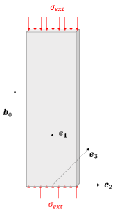
Figure 1: Schematics of the magnetostriction setup.

A thin plate of electrical steel is subjected to an external magnetic field $b_{0}\boldsymbol{e}_{1}$ along its axial direction, resulting in an axial magnetic field $b_{1}=(1+\chi)b_{0}$ (assumed uniform) inside the specimen, where $\chi$ is the material’s magnetic susceptibility. The plate is also subjected to an externally applied uniaxial stress $\sigma_{ext}\boldsymbol{e}_{1}\boldsymbol{e}_{1}$ and hence the total stress $\boldsymbol{\sigma}$ is the sum of the applied stress and the Maxwell stress in vacuum due to the magnetic field ${\boldsymbol{b}}_{0}$

$$\boldsymbol{\sigma}=\overset{e}{\boldsymbol{\sigma}}+\overset{m}{\boldsymbol{\sigma}}=\sigma_{ext}\boldsymbol{e}_{1}\boldsymbol{e}_{1}+\frac{1}{\mu_{0}}\left[{\boldsymbol{b}}_{0}{\boldsymbol{b}}_{0}-\frac{1}{2}({\boldsymbol{b}}_{0}\!\boldsymbol{\cdot}\!{\boldsymbol{b}}_{0})\boldsymbol{I}\right]$$ (C.1)

where the expressions for the elastic and magnetic part of the total stress are given by (2.25). The corresponding strain and the stress fields in the plate are assumed uniform with edge effects near the corners and edges of the plate neglected.

Consequently the resulting axial strain $\epsilon_{11}$ is made of an elastic component $\sigma_{ext}/E$ plus a component proportional to the square of the magnetic field strength $\zeta_{m}(b_{1})^{2}$, where the curvature coefficient $\zeta_{m}$ depends on the magnetic constants (susceptibility $\chi$ and magneto-mechanical coupling $\Lambda$). A straightforward calculation from (C.1) and (2.25), considering that the specimen’s lateral strain is $\epsilon_{22}=\epsilon_{33}$, gives two independent equations

$$(\lambda+2G)\epsilon_{11}+2\lambda\epsilon_{22}=\sigma_{ext}+{{(b_{0})^{2}}\over{2\mu_{0}}}\left[1-(1+\chi)^{2}-2\Lambda(1+\chi)\right]\;,\quad\lambda\epsilon_{11}+2(\lambda+G)\epsilon_{22}=-{(b_{0}\chi)^{2}\over 2\mu_{0}}\;,$$ (C.2)

where the Lamé constants are given in terms of Young’s modulus $E$ and Poisson ratio $\nu$ by $G=E/2(1+\nu)$ and $\lambda=\nu E/(1+\nu)(1-2\nu)$. From (C.2) one obtains the sought relation between the axial strain, the external stress and the magnetic field as well as the expression for the curvature coefficient $\zeta_{m}$

$$\epsilon_{11}={\sigma_{ext}\over E}+\zeta_{m}(b_{1})^{2}\;;\quad\zeta_{m}=\zeta_{m\chi}+\zeta_{m\Lambda}\;,\quad\zeta_{m\chi}\equiv\displaystyle-{({1\over 2}-\nu)\chi^{2}+\chi\over E\mu_{0}(1+\chi)^{2}}\;,\ \zeta_{m\Lambda}\equiv{-\Lambda\over E\mu_{0}(1+\chi)}\;.$$ (C.3)

In decomposing the curvature $\zeta_{m}$ into a magnetic susceptibility $\zeta_{m\chi}$ and a magneto-mechanical $\zeta_{m\Lambda}$ component we follow the approach of Daniel et al. (2003) , where the coefficients $\zeta_{m\chi}$ and $\zeta_{m\Lambda}$ correspond respectively to the magnetic susceptibility $\chi$ and the magneto-mechanical coupling $\Lambda$ parts of the magnetic stress $\overset{m}{\boldsymbol{\sigma}}$ defined in (2.25).

For the no external stress case ($\sigma_{ext}=0$) the data from Aydin et al. (2017), which are based on the approach adopted in Daniel et al. (2003), provide the same magneto-mechanical coupling curvature $\zeta_{m\Lambda}=2\;10^{-6}\;T^{-2}$ for the two materials analyzed. Unfortunately, the values for $\nu$ associated to these materials are not reported there. We assume typical values for steel: $\nu=0.34$, $E=183$GPa and a magnetic susceptibility $\chi=4\;10^{3}$, resulting in $\Lambda\approx-1.8\!\times\!10^{3}$ which is used in our calculations, as seen in Table 1.

References

- Abdel-Razek et al. (1982) Abdel-Razek, A., Coulomb, J., Feliachi, M., Sabonnadiere, J., 1982. Conception of an air-gap element for the dynamic analysis of the electromagnetic field in electric machines. IEEE Transactions on Magnetics 18, 655–659. URL: https://ieeexplore.ieee.org/abstract/document/1061898.
- Arkkio (1987) Arkkio, A., 1987. Analysis of induction motors based on the numerical solution of the magnetic field and circuit equations , 97URL: http://urn.fi/urn:nbn:fi:tkk-001267.
- Aydin et al. (2017) Aydin, U., Rasilo, P., Martin, F., Singh, D., Daniel, L., Belahcen, A., Rekik, M., Hubert, O., Kouhia, R., Arkkio, A., 2017. Magneto-mechanical modeling of electrical steel sheets. Journal of Magnetism and Magnetic Materials 439, 82 – 90. URL: http://www.sciencedirect.com/science/article/pii/S0304885317300859, doi:https://doi.org/10.1016/j.jmmm.2017.05.008.
- Barber (2009) Barber, J., 2009. Elasticity. Solid Mechanics and Its Applications, Springer Netherlands. URL: https://books.google.fr/books?id=5M9j319PbKMC.
- Belahcen et al. (2006) Belahcen, A., Fonteyn, K., Fortino, S., Kouhia, R., 2006. A coupled magnetoelastic model for ferromagnetic materials. Proc. of the IX Finnish Mechanics Days. von Hertzen R., Halme T.(eds.) , 673–682.
- Boules (1984) Boules, N., 1984. Two-dimensional field analysis of cylindrical machines with permanent magnet excitation. IEEE Transactions on Industry Applications IA-20, 1267–1277.
- Brown (1966) Brown, W.F., 1966. Magnetoelastic Interactions. Springer-Verlag, New York.
- Chari and Silvester (1971) Chari, M.V.K., Silvester, P., 1971. Analysis of turboalternator magnetic fields by finite elements. IEEE Transactions on Power Apparatus and Systems PAS-90, 454–464. URL: https://ieeexplore.ieee.org/abstract/document/4074358.
- Coleman and Noll (1963) Coleman, B.D., Noll, W., 1963. The thermodynamics of elastic materials with heat conduction and viscosity. Archive for Rational Mechanics and Analysis 13, 167–178. URL: https://doi.org/10.1007/BF01262690, doi:10.1007/BF01262690.
- Daniel et al. (2020) Daniel, L., Bernard, L., Hubert, O., 2020. Multiscale Modeling of Magnetic Materials. Elsevier.
- Daniel and Hubert (2009) Daniel, L., Hubert, O., 2009. An analytical model for the e effect in magnetic materials. The European Physical Journal Applied Physics 45, 31101.
- Daniel et al. (2003) Daniel, L., Hubert, O., Ossart, F., Billardon, R., 2003. Experimental analysis and multiscale modelling of the anisotropic mechanical and magnetostrictive behaviours of electrical steels, in: Journal de Physique IV (Proceedings), EDP sciences. pp. 247–254.
- Devillers et al. (2016) Devillers, E., Le Besnerais, J., Lubin, T., Hecquet, M., Lecointe, J., 2016. A review of subdomain modeling techniques in electrical machines: Performances and applications, in: 2016 XXII International Conference on Electrical Machines (ICEM), pp. 86–92. URL: https://ieeexplore.ieee.org/abstract/document/7732510.
- Dorfmann and Ogden (2003) Dorfmann, A., Ogden, R., 2003. Magnetoelastic modelling of elastomers. European Journal of Mechanics - A/Solids 22, 497 – 507. URL: http://www.sciencedirect.com/science/article/pii/S0997753803000676, doi:https://doi.org/10.1016/S0997-7538(03)00067-6.
- Fonteyn et al. (2010a) Fonteyn, K., Belahcen, A., Kouhia, R., Rasilo, P., Arkkio, A., 2010a. Fem for directly coupled magneto-mechanical phenomena in electrical machines. IEEE Transactions on Magnetics 46, 2923–2926.
- Fonteyn et al. (2010b) Fonteyn, K.A., Belahcen, A., Rasilo, P., Kouhia, R., Arkkio, A., 2010b. Contribution of maxwell stress in air on the deformations of induction machines, in: 2010 International Conference on Electrical Machines and Systems, pp. 1749–1753.
- Fonteyn et al. (2010) Fonteyn, K.A., et al., 2010. Energy-based magneto-mechanical model for electrical steel sheets .
- Gieras and Saari (2012) Gieras, J.F., Saari, J., 2012. Performance calculation for a high-speed solid-rotor induction motor. IEEE Transactions on Industrial Electronics 59, 2689 – 2700.
- Hiptmair and Ostrowski (2005) Hiptmair, R., Ostrowski, J., 2005. Coupled boundary-element scheme for eddy-current computation. Journal of Engineering Mathematics 51, 231–250. URL: https://doi.org/10.1007/s10665-004-2116-3, doi:10.1007/s10665-004-2116-3.
- Huppunen et al. (2004) Huppunen, J., et al., 2004. High-speed solid-rotor induction machine–electromagnetic calculation and design URL: https://lutpub.lut.fi/handle/10024/36551.
- Hutter et al. (2007) Hutter, K., Ven, A.A., Ursescu, A., 2007. Electromagnetic Field Matter Interactions in Thermoelasic Solids and Viscous Fluids. volume 710. Springer.
- Jackson (1999) Jackson, J.D., 1999. Classical Electrodynamics, 3rd ed. John Wiley & Sons, Inc.
- Javadi et al. (1995) Javadi, H., Lefèvre, Y., Clénet, S., Mazenc, M., 1995. Electro-magneto-mechanical characterizations of the vibration of magnetic origin of electrical machines. IEEE transactions on magnetics 31, 1892–1895. URL: https://ieeexplore.ieee.org/abstract/document/376408.
- Kankanala and Triantafyllidis (2004) Kankanala, S., Triantafyllidis, N., 2004. On finitely strained magnetorheological elastomers. Journal of the Mechanics and Physics of Solids 52, 2869 – 2908. URL: http://www.sciencedirect.com/science/article/pii/S0022509604000821, doi:https://doi.org/10.1016/j.jmps.2004.04.007.
- Kovetz (2000) Kovetz, A., 2000. Electromagnetic theory. volume 975. Oxford University Press Oxford.
- Lefevre and Lopez-Pamies (2017) Lefevre, V., Lopez-Pamies, O., 2017. Homogenization of elastic dielectric composites with rapidly oscillating passive and active source terms. SIAM Journal on Applied Mathematics 77, 1962–1988.
- López et al. (2019) López, I., Ibarra, E., Matallana, A., Andreu, J., Kortabarria, I., 2019. Next generation electric drives for hev/ev propulsion systems: Technology, trends and challenges. Renewable and Sustainable Energy Reviews 114, 109336. URL: http://www.sciencedirect.com/science/article/pii/S1364032119305441, doi:https://doi.org/10.1016/j.rser.2019.109336.
- Lubin et al. (2011) Lubin, T., Mezani, S., Rezzoug, A., 2011. Analytic calculation of eddy currents in the slots of electrical machines: Application to cage rotor induction motors. IEEE Transactions on Magnetics 47, 4650–4659. doi:10.1109/TMAG.2011.2157167.
- Michell (1899) Michell, J.H., 1899. On the Direct Determination of Stress in an Elastic Solid, with application to the Theory of Plates. Proceedings of the London Mathematical Society s1-31, 100–124. URL: https://doi.org/10.1112/plms/s1-31.1.100, doi:10.1112/plms/s1-31.1.100, arXiv:http://oup.prod.sis.lan/plms/article-pdf/s1-31/1/100/4637069/s1-31-1-100.pdf.
- Pao and Yeh (1973) Pao, Y.H., Yeh, C.S., 1973. A linear theory for soft ferromagnetic elastic solids. International Journal of Engineering Science 11, 415 – 436. URL: http://www.sciencedirect.com/science/article/pii/0020722573900591, doi:https://doi.org/10.1016/0020-7225(73)90059-1.
- Rekik et al. (2014) Rekik, M., Hubert, O., Daniel, L., 2014. Influence of a multiaxial stress on the reversible and irreversible magnetic behaviour of a 3% si-fe alloy. International Journal of Applied Electromagnetics and Mechanics 44, 301–315.
- Reyne et al. (1987) Reyne, G., Sabonnadiere, J., Coulomb, J., Brissonneau, P., 1987. A survey of the main aspects of magnetic forces and mechanical behaviour of ferromagnetic materials under magnetisation. IEEE Transactions on Magnetics 23, 3765–3767. URL: https://ieeexplore.ieee.org/abstract/document/1065518.
- Reyne et al. (1988) Reyne, G., Sabonnadiere, J.C., Imhoff, J.F., 1988. Finite element modelling of electromagnetic force densities in dc machines. IEEE Transactions on Magnetics 24, 3171–3173. URL: https://ieeexplore.ieee.org/abstract/document/92371.
- Silvester et al. (1973) Silvester, P., Cabayan, H.S., Browne, B.T., 1973. Efficient techniques for finite element analysis of electric machines. IEEE Transactions on Power Apparatus and Systems PAS-92, 1274–1281. URL: https://ieeexplore.ieee.org/abstract/document/4075205.
- Thomas and Triantafyllidis (2009) Thomas, J., Triantafyllidis, N., 2009. On electromagnetic forming processes in finitely strained solids: Theory and examples. Journal of the Mechanics and Physics of Solids 57, 1391 – 1416. URL: http://www.sciencedirect.com/science/article/pii/S0022509609000465, doi:https://doi.org/10.1016/j.jmps.2009.04.004.
- Tian et al. (2012) Tian, L., Tevet-Deree, L., DeBotton, G., Bhattacharya, K., 2012. Dielectric elastomer composites. Journal of the Mechanics and Physics of Solids 60, 181–198.
- Zhu et al. (1993) Zhu, Z.Q., Howe, D., Bolte, E., Ackermann, B., 1993. Instantaneous magnetic field distribution in brushless permanent magnet dc motors. i. open-circuit field. IEEE Transactions on Magnetics 29, 124–135. URL: https://ieeexplore.ieee.org/abstract/document/195557/references#references.