XLBoost-Geo: An IP Geolocation System Based on Extreme Landmark Boosting

Abstract.

IP geolocation aims at locating the geographical position of Internet devices, which plays an essential role in many Internet applications. In this field, a long-standing challenge is how to find a large number of highly-reliable landmarks, which is the key to improve the precision of IP geolocation. To this end, many efforts have been made, while many IP geolocation methods still suffer from unacceptable error distance because of the lack of landmarks. In this paper, we propose a novel IP geolocation system, named XLBoost-Geo, which focuses on enhancing the number and the density of highly reliable landmarks. The main idea is to extract location-indicating clues from web pages and locating the web servers based on the clues. Based on the landmarks, XLBoost-Geo is able to geolocate arbitrary IPs with little error distance. Specifically, we first design an entity extracting method based on a bidirectional LSTM neural network with a self-adaptive loss function (LSTM-Ada) to extract the location-indicating clues on web pages and then generate landmarks based on the clues. Then, by measurements on network latency and topology, we estimate the closest landmark and associate the coordinate of the landmark with the location of the target IP. The results of our experiments clearly validate the effectiveness and efficiency of the extracting method, the precision, number, coverage of the landmarks, and the precision of the IP geolocation. On RIPE Atlas nodes, XLBoost-Geo achieves 2,561m median error distance, which outperforms SLG and IPIP.

1. Introduction

For the past decades, with network security incidents occur frequently, people have increasingly emphasized on cyberspace security. Due to the critical importance of high-precision IP geolocation in the field of cyberspace security, maintaining cyberspace security has become a main driving force for people to conduct this research.

IP geolocation refers to locating the geographical position of Internet devices, most of which do not have a geolocation function themselves. Even for devices with GPS modules, to protect privacy or cover up illegal behavior, they would not share geographical position. Hence, locating Internet devices through IP address becomes one of the most important approaches to discover their geographical position.

However, a critical challenge for IP geolocation is how to improve the number of landmarks, Internet devices with a known geographical position. Although existing IP geolocation methods have made great progress, there is still much room for further improvement in positioning precision. Many IP geolocation approaches with high precision rely heavily on the density of landmarks. For example, network measuring based methods, like street-level geolocation (SLG(Wang et al., 2011a)), map a target device to the nearest landmark’s location. Data mining based methods, like Structon(Guo et al., 2009) and Checkin-Geo(Liu et al., 2014), mine landmarks and expand the coverage by clustering IPs. Existing methods that claim to have achieved thousands or hundreds of meters medium error distance (MED), still influenced by regional imbalance and provide unreliable results in regions with sparse landmarks. Therefore, enhancing the number of landmarks is the key to further improve the performance of IP geolocation system.

Figure 1. A motivating example: to find potential landmarks as more as possible, by which we can improve the estimation precision

To this end, in this paper, we design a novel IP geolocation system, named XLBoost-Geo, focusing on enhancing the number and the density of highly reliable landmarks, which we refer to as landmark boosting. Figure 1 shows a motivating example of our IP geolocation system. As we can see, through network measuring, we can find the closest landmark to the target device and map its location to the target as an estimated position. If the bold circles are all landmarks that we can get by previous methods, we can get a position with error distance as $r_{1}$. However, there are still many potential landmarks (shown as dashed circles) left, which can be mined to further decrease the estimation error of IP geolocation. Therefore, an ideal scenario of XLBoost-Geo is that it can find potential landmarks as more as possible so that we can map the target device to a closer landmark’s location. In this case, we can lower the error to $r_{2}$ as shown in Figure 1.

In order to mine a large volume of landmarks in a cost-effective way, XLBoost-Geo extracts geographical location clues from web pages on locally deployed web servers. Due to a strong association between the position of local web servers and location clues on their web pages, many previous IP geolocation methods (e.g. SLG(Wang et al., 2011a) and Structon(Guo et al., 2009)) mine landmarks based on this association, but they do not fully utilize this kind of open resources. SLG uses keywords and zipcodes to search for landmarks by mapping services. Even though this method can generate a set of landmarks with a highly precise location, the number is limited because it is hard to cover all possible keywords and maps only include the main portal website for each organization, which is usually hosted on cloud servers and thus can not be used as a landmark. Structon mines geolocation information from 500 million pages, which is large enough to generate plenty of landmarks. However, it uses regular expressions for geolocation extraction, which is able to extract coarse-grained geolocation items, such as city, province, and state, but not street-level and building-level ones. Because of defects during their mining process, the number of landmarks SLG mined is limited, and the location of landmarks mined by Structon is very coarse and can only achieve city-level precision.

Different from the aforementioned two approaches, XLBoost-Geo scans all addresses in IPv4 space to crawl web pages that contain location-indicating clues. XLBoost-Geo extracts the clues as precise as possible by a variant of the state-of-the-art entity extraction model. For web servers with explicit location information (e.g. contact address) on the web pages, XLBoost-Geo extracts and geocode the complete address to geographical coordinates directly. For those without contact addresses, XLBoost-Geo utilizes implicit clues (e.g. owner name extracted from copyright, title, and logo), which are ignored by previous works, to infer the coordinate. Therefore, XLBoost-Geo is able to boost the number of highly reliable landmarks by extremely making use of clues on web pages.

Figure 2 shows the framework of XLBoost-Geo. Specifically, given an IP segment, we first scan and detect IPs that expose HTTP/HTTPS relevant ports by MASSCAN(mas, [n.d.]). Then, we extract these IPs’ organization name from Whois register information and filter locally deployed web servers by a blacklist of proxy providers. Next, we crawl the home pages and contact pages of the local web servers as raw resources for extracting location-indicating clues. Inspired by LSTM-LSTM-Bias(Zheng et al., 2017), the state-of-the-art model for joint extraction, we design a novel location-indicating clue extracting method based on bidirectional LSTM neural network with a self-adaptive loss function (LSTM-Ada). To supplement the owner names that the LSTM-Ada model fails to extract, we use an organization dictionary (refer to Appendix C) to help. With these clues, we can yield a landmark database by mapping services and further expand the landmark database by a measurement-based coordinate selection algorithm. Based on these landmarks, XLBoost-Geo can locate a target IP by associate the target with the nearest landmark’s position.

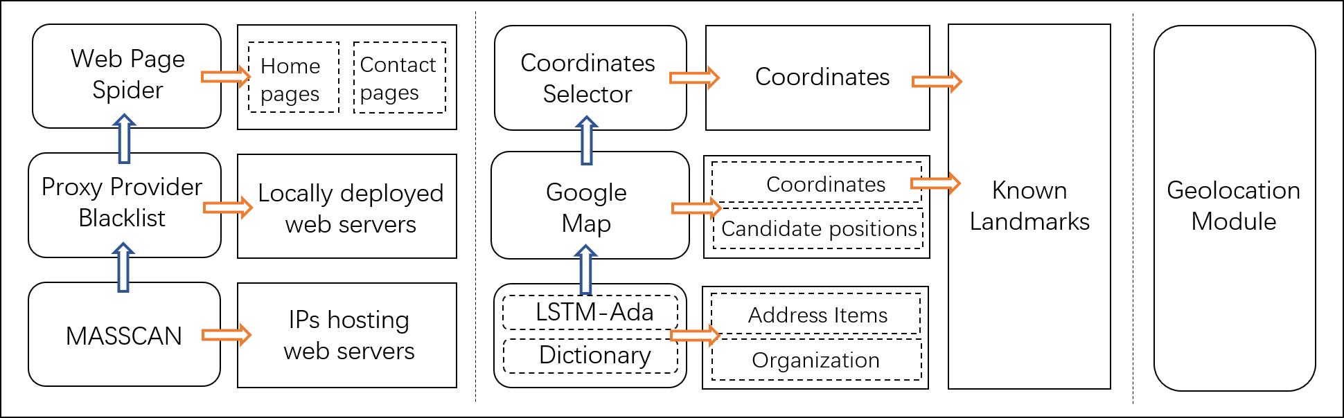
Figure 2. The framework of XLBoost-Geo

Finally, we conduct extensive experiments on real-world IP geolocation tasks. The results clearly validate the effectiveness and the precision of XLBoost-Geo, which has been deployed in a real-world commercial IP geolocation system, named IPPLUS360, which was originally developed based on SLG(Wang et al., 2011a). XLBoost-Geo receives remarkable performances in terms of efficiency of landmark mining and enhances the locating precision of IPPLUS360 to a large degree.

2. XLBoost-Geo

2.1. Data Mining Based Landmark Generation

To construct our landmark database, we first scan a batch of IPs and find out Web servers by detecting HTTP/HTTPS relevant ports. Second, we query the organizations of the IPs by Whois database. Then, by a proxy provider blacklist, we filter out proxy servers which are not hosted locally. The blacklist was generated by manual collection and a classifier trained by Wikipedia description. Since location-indicating clues are only exposed on home pages and contact pages, we only crawl these pages from the local Web servers as raw data. Third, inspired by the state-of-the-art joint extraction model, namely LSTM-LSTM-Bias, we design a variant model with self-adaptive loss function (LSTM-Ada) to extract location clues from the web pages. Finally, based on the clues, we deduce the locations of the web servers and map them to their corresponding IP. The first two steps are easy to implement and not the focus of this paper, so this section details the last two steps.

To extract location clues, we model the process as a sequence tagging task. Since the LSTM-based end-to-end model is widely used in this task and has been shown the effectiveness, we use Bi-LSTM as the main structure of both the encoding layer and the decoding layer. Different from previous models, we employ a self-adaptive loss function that is able to adjust the weights of tags in each training epoch. The self-adaptive loss function has the model more focus on tough-to-extract clues and thus it can enhance the performance of extracting address information on the pages, especially the detailed address (street-level or building-level location-indicating clues). The detailed address is harder to extract than the other location-indicating clues due to its diverse patterns.

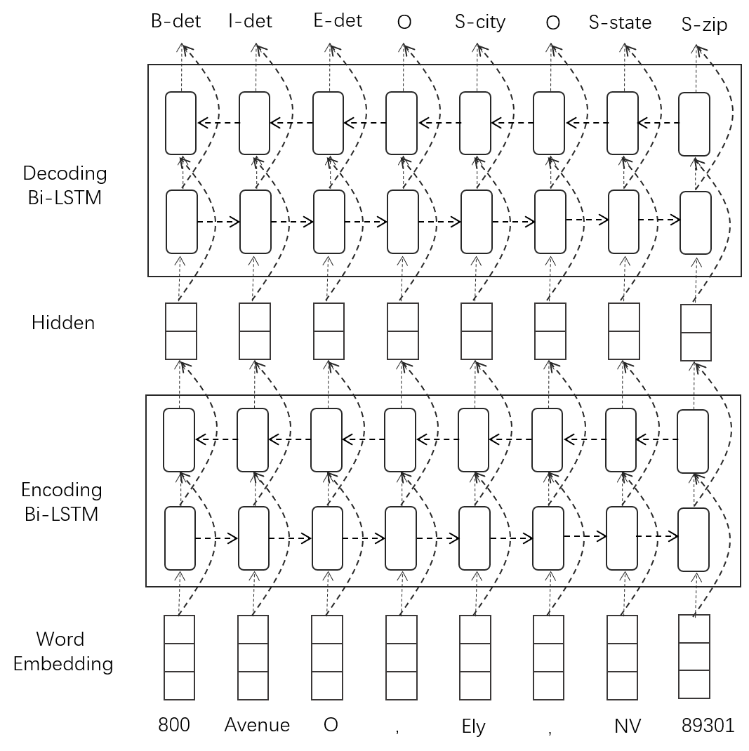
Figure 3. The structure diagram of LSTM-Ada

The structure diagram of the model is shown in Figure 3. The inputs are one-hot vectors of words and the outputs are predicted tags that contribute to extract the location-indicating entities in the page text. The word embedding layer converts the one-hot vector to an embedding vector. Hence, by the word embedding layer, a text can be represented as $S={x_{1},...,x_{t},...,x_{n}}$, where $x_{t}$ is the embedding vector corresponding to the t-th token in the sentence. After the word embedding layer, there is a Bi-LSTM encoding layer, which consists of two parallel LSTM layers: forward LSTM layer and backward LSTM layer. The LSTM architecture consists of a set of recurrently connected memory blocks, referred to as cells. The cell in Bi-LSTM encoding layer is used to compute current hidden vector $h_{t}$ based on the previous hidden vector $h_{t-1}$, the previous cell vector $c_{t-1}$ and the current input embedding vector $x_{t}$. The detail operations for updating hidden state $h_{t}$ are defined as follows:

(1) $$i_{t}=\sigma(W_{i}h_{t-1}+U_{i}x_{t}+b_{i})$$

(2) $$f_{t}=\sigma(W_{f}h_{t-1}+U_{f}x_{t}+b_{f})$$

(3) $$\tilde{c_{t}}=\tanh{(W_{c}h_{t-1}+U_{c}x_{t}+b_{c})}$$

(4) $$c_{t}=f_{t}\odot c_{t}-1+i_{t}\odot\tilde{c_{t}}$$

(5) $$o_{t}=\sigma(W_{o}h_{t-1}+U_{o}x_{t}+b_{o})$$

(6) $$h_{t}=o_{t}\odot\tanh{(c_{t})}$$

Here, $\sigma$ is the element-wise sigmoid function and $\odot$ is the element-wise product. $U_{*}$ and $W_{*}$ denote the weight matrices and $b_{*}$ are the bias terms. $x_{t}$ is the word embedding vector at time $t$, and $h_{t}$ is the hidden state vector storing contextual information. For each word embedding vector $x_{t}$, the forward LSTM layer will encode $x_{t}$ to $\overrightarrow{h_{t}}$ by considering the contextual information from $x_{1}$ to $x_{t}$. The backward LSTM applys the same logic backward and yield $\overleftarrow{h_{t}}$, which contains contextual information from $x_{n}$ to $x_{t}$. Finally, we concatenate $\overrightarrow{h_{t}}$ and $\overleftarrow{h_{t}}$ to represent word t’s encoding information, denoted as the bidirectional hidden state $\hat{h_{t}}$ = [$\overrightarrow{h_{t}}$; $\overleftarrow{h_{t}}$].

We also employ a Bi-LSTM structure for the decoding layer. All the hidden states $\hat{h_{t}}$ obtained from the Bi-LSTM encoding layer are fed into the Bi-LSTM decoding layer to produce the tag sequence. The operations for calculating the hidden state $h_{t}$ in the decoding layer are the same as the one in the encoding layer. Based on the $\hat{h_{t}}$ obtained from the Bi-LSTM decoding layer, the final fully connected layer (FCL) with softmax function computes normalized entity tag probabilities as follows:

(7) $$y_{t}=W_{y}\hat{h_{t}}+b_{y}$$

(8) $$p_{t,i}=\frac{e^{y_{t,i}}}{\sum_{j=1}^{N}e^{y_{t,j}}}$$

Above, $W_{y}$ is the weight matrix and $b_{y}$ is the bias term. $N$ is the total number of tags. $y_{t,j}$ is the j-th element of $y_{t}$, which is an N-dimension vector output by the FCL. $p_{t,i}$ is the score of assigning the t-th word with the i-th tag.

During training, we use Adam(Kingma and Ba, 2014) to maximize the log-probability of the data. The objective function is defined below:

(9) $$L=-\sum_{s=1}^{|D|}\sum_{t=1}^{T}w\odot\hat{y}_{t}^{s}\sum_{j=1}^{N}\hat{y}_{t,j}^{s}log(p_{t,j}^{s})$$

(10) $$w_{i}=exp(\alpha(\frac{1}{N}\sum_{j=1}^{N}{F_{1}}^{j}-{F_{1}}^{i}))$$

Here, $|D|$ is the size of a batch of data, $T$ is the length of a page text, $N$ is the number of tags, $\hat{y}_{t}^{s}$ is the one-hot vector of the true label of the t-th word in the s-th text, and $\hat{y}_{t,j}$ is the j-th element of $\hat{y}_{t}^{s}$. Besides, $w_{i}$ is the i-th element of $w$, which is the weight vector of tags, ${F_{1}}^{i}$ is the $F_{1}$ score of the i-th tag on the validation set in the last epoch, and $\alpha$ is the coefficient of distinguishing, which adjusts the degree of distinguishing the weights of tags.

During the inference, we label each word as the tag with the highest score. For each page text, we obtain a tag sequence from the model, based on which we can extract location-indicating entities from the page text. We use the “BIESO” (Begin, Inside, End, Single, Other) signs to represent a word’s position in the entity. The tag ”O” means that the corresponding word has nothing to do with the location-indicating entity. Different from “O”, the other tags consist of two parts: the word position in the entity and the entity type, which are concatenated using a dash. As shown in Figure 3, the text ”800 Avenue O, Ely, NV 89301” is fed into the model to output the tag sequence B-det, I-det, E-det, O, S-city, O, S-state, S-zip, which means ”800 Avenue O” is the detailed address, ”Ely” is a city, ”NV” is a state, and 89301 is a ZIP code.

Now given a web page with contact information and copyright information, we can extract at most 5 kinds of location-indicating items, including organization name, ZIP code, state, city, street-level or building-level address (detailed address for short). Figure 1 also exemplifies these location-indicating items. If a web page contains these 5 items, we can extract all of them in most cases with LSTM-Ada. Then, we can order them into a formatted address and geocode it to a geographical coordinate by a mapping service(e.g. Google Map). In fact, full information is not a must. Four-Tuple (detailed address, city, state, ZIP code) is enough to decide a coordinate. In other words, if a page contains full contact information, the organization name is not necessary.

However, Our experiment results show that the detailed address is the bottle-neck of the extraction process but the organization name is more common and easier to extract. Plus, an organization usually has only one or several subsidiaries in a small region. Therefore, if a web page only exposes the organization name but not contact information, or if LSTM-Ada fails to extract the full contact information, especially the detailed address, the organization name will play its magic in the geolocation process. If any clues indicating a small region, e.g. state, city, or ZIP code, can be successfully extracted, we can, through a map, look up several possible coordinates in the region with the organization name as a keyword. If the model fails to extract any region-indicating clues, we use a variant of CBG(Gueye et al., 2006a) (refer to Appendix B) to help determine possible coordinates. If there is only one possible coordinate returned, we map it to the IP directly. If there is more than one possible coordinate returned, we leave the rest tasks to the coordinate selection algorithm which is mentioned in Section 2.2.

2.2. Coordinate Selecting Algorithm Based Landmark Generation

If a possible region is determined, and there is more than one possible coordinate in the region, we will select the most possible one based on measurements. This algorithm is based on two assumptions. First, The closer the two Internet devices are the closer the delays from the same probe to them. Second, The closer the two Internet devices are, the shorter the route from one to another. Even though these two assumptions are not always true, they work very well in previous IP geolocation methods, e.g. CBG, SLG, and etc.

This algorithm mainly includes four steps. First, in the vicinity of possible coordinates, select a set of landmarks and a set of probes for estimating the distance between each landmark and the target IP. Second, score the landmarks based on the estimated distance to the target IP. Third, deliver the score from landmarks to the candidate coordinates according to the geographical distance. Finally, select the location with the highest score and map it to the target IP. Based on the two assumptions mentioned above, we estimate the distance between each landmark and the target IP by calculating the similarity between the delay vectors and computing the length of the shortest route. As for the geographical distance between a landmark and each candidate coordinate, we obtain it by calculating the great circle distance (Vincenty, 1975) between the two coordinates.

Formally, the score of a candidate coordinate can be calculated as below:

(11) $$score({c_{i}})=\sum\nolimits_{{l_{j}}\in L}{g({l_{j},c_{i}})}{s({l_{j}})}$$

Here, $s(l_{j})$is the score of each landmark$l_{j}$ and $g(l_{j},c_{i})$is the redistributing gate, which play the role of delivering a weighted $s(l_{j})$ to every candidate coordinate $c_{i}$. The weight is based on the distance between the landmark and the candidate coordinate.

As mentioned before, a candidate should get a higher score from a landmark if it is closer to the landmark than the others. Therefore, the redistributing gates are defined below:

(12) $$g({l_{j},c_{i}})=1-\frac{e^{dis({c_{i}},{l_{j}})}}{{\sum\nolimits_{{l_{k}}\in L}{{e^{dis({c_{i}},{l_{k}})}}}}}$$

Here, $c_{i}$ represents a candidate coordinate, $l_{i}$ represents a landmark, and $dis(c_{i},l_{i})$ refers to the great circle distance between them.

Based on the two previously mentioned assumptions, we use the following formula to calculate the score of each landmark:

(13) $$s({l_{i}})=\alpha\cdot{s_{d}}({l_{i}})+\beta\cdot{s_{t}}({l_{i}})$$

Above, ${s_{t}}({l_{i}})$ and ${s_{d}}({l_{i}})$ represent the score of a landmark in the perspective of topology and the perspective of pure network delay measurement. The former is decided by the length of the shortest route from the landmark to the target IP. The latter is decided by the similarity between the delay vector of the landmark and the delay vector of the target IP. $\alpha$ and $\beta$ are the weights of ${s_{d}}({l_{i}})$ and ${s_{t}}({l_{i}})$ separately.

The score of a landmark in the perspective of pure network delay measurement can be calculated as following two formulas:

(14) $${s_{d}}({l_{i}})=\frac{sim({l_{i}},t)}{\sum\nolimits_{{l_{j}}\in L}{sim({l_{j}},t)}}$$

(15) $$sim({l_{i}},t)=\frac{{\boldsymbol{v}_{l_{i}}}{\boldsymbol{v}_{t}}}{\left|{\boldsymbol{v}_{l_{i}}}\right|\left|{\boldsymbol{v}_{t}}\right|}$$

${v}_{l_{i}}$ and ${v}_{t}$ denote the delay vector of a landmark and the target IP separately. Each element in the vectors is the delay measured from a probe. ${sim({l_{i}},t)}$ represents the cosine similarity between ${v}_{l_{i}}$ and ${v}_{t}$.

The score of a landmark in the perspective of topology can be calculated as below:

(16) $${s_{t}}({l_{i}})=1-\frac{{e^{r({l_{i}},t)}}}{\sum\nolimits_{{l_{j}}\in L}{{e^{r({l_{j}},t)}}}}$$

$r({l_{i}},t)$ denotes the length of the shortest route between a landmark $l_{i}$ and the target IP $t$. Inspired by (Wang et al., 2011a), we approximately calculate the shortest route by finding the closest common router. Figure 4 illustrates an example, we first send traceroute probes to the landmark $L_{1}$ and the target host $H_{1}$ from all probes ($P_{1}$, $P_{2}$, and etc.). For each probe, we then find the closest common router to $H_{1}$ and $L_{1}$, shown as R2 and R4 in Figure 4. Through the common routers (R2 and R4), The routes passing from $L_{1}$ to $H_{1}$ is the approximate indirect route. In Figure 4, The indirect route $r_{1}$ is $L_{1}$ -¿ $R_{2}$ -¿ $R_{3}$ -¿ $H_{1}$, and the indirect route $r_{2}$ is $L_{1}$ -¿ $R_{4}$ -¿ $H_{1}$. We separately sum the delays on the routes as the their length. Since $e_{4}$ + $e_{5}$ is shorter than $e_{3}+e_{7}+e_{8}$, we take the former as the length of the shortest route.

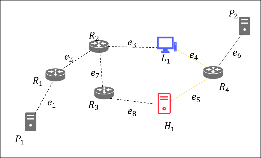
Figure 4. To approximately calculate the length of the shortest route by finding the closest router

2.3. IP Geolocation Based on Landmarks

Based on the landmarks mined by the aforementioned method, XLBoost-Geo is able to geolocate an arbitrary IP. The main idea is to find the closest landmark to the target IP and take the location of the landmark as an estimate of the target IP. First, select a set of probes that closest to the target IP based on the assumption that the smaller the delay, the closer the probe to the target. Second, calculate the scores of all landmarks according to Formula 14 and select a set of candidate landmarks with the highest scores. Third, calculate the scores of the candidate landmarks according to Formula 16 and sum two scores together as Formula 13. Then, select the landmark with the highest score as the closest landmark.

3. Experimental Result

3.1. The Performance of Location-indicating Clue Extraction

Data Description: As previously mentioned, we use LSTM-Ada to extract the location-indicating clues on web pages. To evaluate the performance of our model, we produce a web page dataset, namely WPLICE (Web Pages for Location-indicating Clues Extraction), which consists of 269,566 web pages that contain location-indicating clues. These pages are crawled from yellow pages websites and web mapping services, which record plenty of organizations with their website, address, and name. To prepare this dataset for training, validating, and evaluation, we extract texts from the web pages and semi-automatically labeled the location-indicating entities on the texts. When it comes to ”semi-automatically”, we mean automatically labeling the page texts based on the organization name and address information revealed and then revising the labels manually. We split this dataset into a train set and a test set by ratio 7:3 and randomly sample 10% data from the test set for validating and choosing the best model.

Experimental Setup: In the experiment, we adopt standard Precision (Prec), Recall (Rec) and F1 score to evaluate the performance of our model. To highlight the strengths of our model in the location-indicating entity extraction task, we compare its performance with two popular sequence tagging models, LSTM-CRF and LSTM-CNN. To highlight the key role of the self-adaptive loss function, we not only calculate the scores on overall extraction results but also calculate the scores of different kinds of tags.

Hyper-parameters: We use FastText(Bojanowski et al., 2017) to pre-train the word embeddings on 22,294,645 web page texts and 11,073,587 addresses. The dimension of the embedding vector is set to 50. The dimension of the embedding layer is also set to 50 and initialized by the embeddings trained by the FastText, the number of units of the Bi-LSTM encoding layer is set to 256 and the number of units of the Bi-LSTM decoding layer is set to 512. The distinguishing coefficient $\alpha$ corresponding to the results in Table 1 is 64. The model is first optimized by using Adam(Kingma and Ba, 2014) and then fine-tuned by using stochastic gradient descent (SDG). Refer to Appendix A.2 for more details about setting hyper-parameters.

Table 1. The performance of location-indicating entity extraction on WPLICE

Models	Results	Prec	Rec	F1	Acc
	all types	0.9757	0.9715	0.9736	-
	organization	0.9771	0.9683	0.9727	0.9632
	detailed	0.9728	0.9536	0.9631	0.9416
LSTM-CRF	city	0.9721	0.9666	0.9693	0.9641
	state	0.9811	0.9827	0.9819	0.9867
	ZIP code	0.9799	0.9795	0.9797	0.9734
	full info	-	-	-	0.8882
	all types	0.9764	0.0.9688	0.9725	-
	organization	0.9780	0.9662	0.9720	0.9698
	detailed	0.9731	0.9546	0.9637	0.9422
LSTM-CNN	city	0.9716	0.9625	0.9670	0.9628
	state	0.9829	0.9789	0.9809	0.9842
	ZIP code	0.9775	0.9756	0.9765	0.9737
	full info	-	-	-	0.8792
	all types	0.9690	0.9812	0.9750	-
	organization	0.9689	0.9798	0.9743	0.9675
	detailed	0.9682	0.9752	0.9716	0.9661
LSTM-Ada	city	0.9692	0.9775	0.9732	0.9682
(our model)	state	0.9694	0.9942	0.9816	0.9874
	ZIP code	0.9724	0.9822	0.9772	0.9786
	full info	-	-	-	0.8937

Results and analysis: The performances on location-indicating entity extraction are shown in Table 1. In the table, Acc denotes the accuracy at page-level, which can be calculated by Formula 17, where $P_{s}uc$ denotes the number of web pages of which the clue is successfully extracted, and $P_{t}otal$ denotes the number of total pages. Besides, ”all types” means to calculate scores without distinguishing each entity type, and ”full info” means all 5 types of entities need to be extracted from the page. Clearly, we observe that our model outperforms the other two models on ”detailed address” and ”full info”, which demonstrates the effectiveness of the self-adaptive loss function. As the function helps to focus on tough-to-extract entities, especially the entities of the detailed address, it help the model improve the success rate of extracting the full location-indicating information. Besides, we use FastText to train word embeddings, which also take into account character-level features, thus the LSTM-CNN has little competitive edges. The dataset is huge enough for the LSTM to learn the transition rules of the tags, so the CRF layer provides little advantages to the model LSTM-CRF. Since the more location-indicating information we get the more precise the location we can get, we use LSTM-Ada to extract location-indicating clues.

(17) $$Acc=\frac{P_{s}uc}{P_{t}otal}$$

3.2. The Performance of Landmark Mining

Data Description: For evaluating the accuracy of the locating of our landmark mining method, we collected data about web servers on PlanetLab to generate the ground-truth dataset. Since the nodes on this Platform report their websites and geographic coordinates, we compare the coordinate estimated by our method and the one shown on PlanetLab. We map the websites to IPs by DNS and remove nodes not locally deployed by the proxy blacklist. Since cross-language problems on entity recognition are not what this paper’s focus, we select the nodes located in the United States to only deal with English websites for convenience. Finally, we got 104 nodes left. We referred to this dataset as PlanetLab-104.

To show the number, coverage, and density of the landmarks that XLBoost-Geo is able to mine, we scaned 1.5 billion IPs of the US by MASSCAN and discovered 6,716,338 local web severs. We crawled home pages and contact pages from these nodes and totally got 8,723,627 pages as the raw data for mining. We referred to this dataset as WebPages-8M.

Experiment Setup: In this section, we show the results of two experiments. For PlanetLab-104, we adopt median error distance (MED), which is commonly used in previous work, to evaluate the accuracy of the estimated location. For comparison, we select a commercial tool IPIP and the state-of-the-art IP geolocation method SLG as baselines. Besides, we mine landmarks from the WebPages-8M and compare the number of landmarks with the ones mined by SLG’s landmark mining method, which is based on keywords and ZIP code. In the experiments, we set to 100 the number of probes in the measurements for the CBG variant(Section 2.1). In coordinate selection algorithm(Section 2.2), We set to 200 the number of probes and set to 1000 the maximum number of the landmarks that closest to the candidate coordinates. Since some intermediate hops do not respond in some cases, the probes can not detect the complete routes to the target and landmarks. In the Formula 13, if ${s_{t}}({l_{i}})$ is not available owing to the incomplete route, $\alpha$ and $\beta$ are set to 1 and 0 separately. In normal cases, both of them are set to 0.5 in XLBoost-Geo.

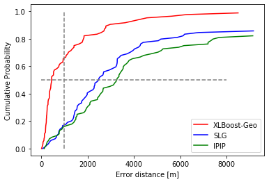
Figure 5. The cumulative distribution function of the error distance on PlanetLab-104

Results and analysis: The performance of the accuracy is shown in Figure 5. As the figure shows, XLBoost-Geo outperforms SLG and IPIP on the estimation accuracy. Specifically, the MED of XLBoost-Geo, SLG, IPIP are 441m, 2,446m, 3,242m respectively (the grey horizontal dashed line). In the results provided by XLBoost-Geo, the percentage of nodes with less than 1km error distance is more than 60, which is more than 3 times as the other two methods (the grey vertical dashed line). The above results demonstrate that XLBoost-Geo has the ability to mine highly-reliable landmarks with little location error. We totally got 1,115,076 landmarks by XLBoost-Geo from the WebPages-8M. Figure 6 shows the distribution of the landmarks in the mainland. As shown by the Figure, except for the Midwest where there are few inhabitants, the eastern and western coastal landmarks are very dense. Besides, The landmarks cover 87% counties in the mainland. The above results show the ability of XLBoost-Geo to mine a large number of and widespread landmarks. Besides, Group by 10 randomly selected ZIP codes, Table 2 shows the comparison of the number of landmarks between the landmark mining method of XLBoost-Geo and SLG’s landmark mining method. In the table, $X$ and $S$ are the abbreviations of XLBoost-Geo and SLG separately, and POI represents ”Point of Interests” searched by map services. After collecting POIs with keywords, SLG’s method has to remove non-locally deployed nodes from the POIs to filter valid landmarks. As the result shows, SLG’s method can only mine tens of landmarks per ZIP code. In contrast, XLBoost-Geo can mine hundreds. The intuitive reason is that SLG’s method is limited by the keywords they use and the number of websites on the web map. This result shows the distinguished efficiency of XLBoost-Geo on landmark mining.

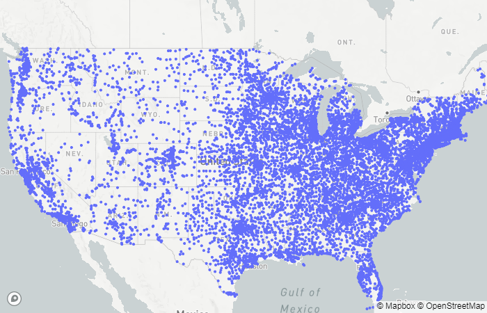
Figure 6. The distribution of the landmarks in the mainland of the US

Table 2. The comparison of the number of landmarks grouped by ZIP codes.

ZIP code	Landmarks-X	POI	Landmarks-S
60007	210	20	6
10018	142	9	1
10017	129	28	8
10036	126	16	0
10022	125	27	5
91730	115	20	4
20005	111	17	4
20036	111	21	4
10001	108	26	3
10016	100	24	4

3.3. The Performance of IP Geolocation

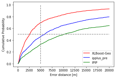
Figure 7. The cumulative distribution function of the error distance on RIPE-Atlas-1156

Data Description: For evaluating the performance on IP geolocation, we collected the ground-truth dataset from RIPE Atlas. RIPE Atlas is the RIPE NCC’s global network of probes that actively measure Internet connectivity. The Members are required to report the coordinates of the probes they own, so we can easily get a lot of ¡IP, coordinate¿ pair from the platform. We select 1156 nodes located in the US to form our dataset, called RIPE-Atlas-1156. This dataset consists of nodes in different network scenes (Table 3), including residential network (306), corporate private network (414), schools (143), data centers (217), and other organizations (76).

Experiment Setup: The same as PlanetLab-104, we adopt MED as the metric to evaluate the accuracy of the estimated location. For comparison, we select IPIP and SLG as baselines. In the experiments, we set to 200 the number of probes and set to 1000 the number of the candidate landmarks. We deal with $\alpha$ and $\beta$ (Formula 13) the same way as we do in the coordinate selection algorithm.

Results and analysis: As shown in Figure 7, XLBoost-Geo outperforms SLG and IPIP on the estimation accuracy. Specifically, the MED of XLBoost-Geo, SLG, IPIP are 2,561m, 5,828m, 10,121m respectively (the grey horizontal dashed line). As for XLBoost-Geo, SLG, and IPIP, the percentages of nodes with less than 5km error distance are 63, 46, 32 separately (the grey vertical dashed line). The figure demonstrates that even for a dataset consist of nodes in varied network scenes, XLBoost-Geo has the ability to geolocate an IP in high precision. To be more specific, Table 3 shows the performance on nodes in each network scene. In the table, $X$, $S$, and $I$ denotes ”XLBoost-Geo”, ”SLG”, and ”IPIP” separately. As shown, XLBoost-Geo outperforms SLG and IPIP in all network scenes, especially the data centers and other organizations, which speaks for the important role of the organizations’ locally-deployed web servers and also indicates that there are many locally-deployed web servers in the vicinity of data centers. Even though SLG performs as well as XLBoost-Geo and achieves 625 MED on school nodes, due to the regional imbalance of landmarks, it fails to achieve the same precision on PlanetLab-104, which also consists of web servers in Universities. In contrast, XLBoost-Geo achieves similar precision on both PlanetLab-104 and these 143 school nodes. According to the above results, XLBoost-Geo mitigates the negative impact of regional imbalance.

Table 3. The performance in each network scene.

Scenario	Num	$MED_{X}$	$MED_{S}$	$MED_{I}$
residential network	306	3,711	5,410	11,255
corporate private network	414	2,806	6,469	12,300
data centers	217	1,903	6,811	8,059
schools	143	491	625	4,179
other organizations	76	1,402	6,670	9,067
total	1156	2,561	5,828	10,121

4. Related Work

4.1. Entity Extraction

In our study, the landmark mining process relies heavily on the accuracy of location clues extracted from web pages. In other words, an efficient and reliable algorithm to extract accurate location clues plays an important role in our study. In our approach, we model the clue mining task to an entity extraction task, which targets at locating location clues in the textual content on web pages. In the past, Entity extraction has been widely studied by researchers. Traditional algorithms, e.g., Hidden Markov Model(Zhou and Su, 2002) and Conditional Random Fields (CRF)(Passos et al., 2014), usually rely on high-quality hand-crafted features and well-designed models. Recently, with the fast development and popularity of deep learning, several neural network-based sequential token tagging techniques have been proposed to address entity extraction tasks, which requires little manual labor to do feature engineering but achieved better performance. For instance, Lample et al.(Lample et al., 2016) combine bidirectional Long Short-Term Memory networks (Bi-LSTM) and CRF for named entity recognition. Chiu et al. use a hybrid Bi-LSTM and Convolutional Neural Network (CNN) to consider both word-level and character-level features(Chiu and Nichols, 2016).

4.2. IP Geolocation

IP geolocation methods can be simply divided into two categories: 1) Data mining-based Methods and 2) Measurement-based Methods. Data mining based methods are measurement-independent and only rely on mining location clues in source data to locate a target IP. These methods are easy to implement but the precision and the coverage are limited by mining methods and the quality of the source data. Measurement-based methods, which rely on network measurements, are universally applicable to nodes that allow ICMP requests. These methods can cover more IPs than data mining-base methods but suffer from higher computational overhead.

Data Mining-based Methods: Since regional Internet registry databases(Whois databases) include the address of the organization of a target IP, Moore et al.(Moore et al., 2000) query and extract the address as the location of the target IP. Since a domain name can contain different granular descriptions of geographic location information, like the abbreviation of a city, state, or country, by mining this information, the geographic location of the target device can be inferred. Based on this idea, GeoTrack(Padmanabhan and Subramanian, 2001), DRoP(Huffaker et al., 2014), rDNS-Geo(Dan et al., 2018) and HLOC(Scheitle et al., 2017) mine location clues in domain names to estimate a location. Structon (Guo et al., 2009) uses regular expressions to extract address information from web pages. By mapping addresses to the corresponding IPs of the web servers, it generates hundreds of thousands of landmarks with city-level precision. GeoCluster (Padmanabhan and Subramanian, 2001) uses the address prefixes(AP) in BGP routing tables to cluster IP addresses and then deduce the entire cluster by location information of a few hosts in a cluster. The location information is extracted from three sources, including login and registration information of Hotmail users, HTTP cookies of bCentral, and users’ query of FooTV. Checkin-Geo (Liu et al., 2014) leverages the location data shared by users in location-sharing services and logs of user logins from PCs for real-time and accurate geolocation. Dan et al.(Dan et al., 2016) generate a large ground-truth dataset using real-time global positioning data extracted from search engine logs. Using the dataset, they measure the accuracy of three commercial IP geolocation databases. Plus, they introduce a technique to improve existing geolocation databases by mining explicit locations from query logs. Based on a crowd-sourcing idea, Lee et al.(Lee et al., 2016) propose an IP geolocation database creation method utilizing Internet broadband performance measurement tagged with locations, and they present an IP geolocation database based on 7 years of Internet broadband performance data in Korea.

Measurement-based Methods: GeoPing (Padmanabhan and Subramanian, 2001) maps a node to the nearest probe’s location based on the measured delays from probes to the node. CBG (Gueye et al., 2006a) utilizes a set of probes to measure a set of delays to a target IP. Based on the delays and delay-distance relation, CBG draws a set of constraint circles, of which the overlap region is where the target IP resides. TBG (Katz-Bassett et al., 2006) claims that routers nearby landmarks are easy to locate and network topology can be effectively leveraged to improve previous IP geolocation techniques. Based on CBG, Octant (Wong et al., 2007) takes both positive and negative measurement constraints into account when estimating a target’s position. Ciavarrini et al.(Ciavarrini et al., 2015)(Ciavarrini et al., 2017) devised an active IP geolocation method that uses smartphones as landmarks based on crowd-sourcing principles: a number of users participate voluntarily to the system and provide their devices as measuring devices. Wang et al.(Wang et al., 2011b) utilize zip codes and keywords to generate passive landmarks through mapping services. They compute the indirect delay between a target and landmarks by finding the closest common routers. Then, they find a landmark with the minimum indirect delay to the target IP and associate the target’s location with it.

Probability and statistics-based methods aim to study the relation between network delay and great circle distance and decrease the error introduced by the delay-distance model. Typical algorithms based on probability and statistics mainly include Posit(Eriksson et al., 2012), Spotter(Laki et al., 2011), GBLC(Zhu et al., 2016), etc. They do not assume that there is a linear relationship between network delay and geographical distance but estimate the statistical relationship between them through statistical analysis of delay-distance data.

The main idea of Machine learning based methods is to reduce IP geolocation to a machine-learning classification problem. Typical machine learning based methods includes LBG(Eriksson et al., 2010), ELC(Maziku et al., 2012), CBIG(Biswal et al., 2014), and NN-Geo(Jiang et al., 2016). LBG(Eriksson et al., 2010) is a Naive Bayes estimation method that assigns a given IP target to a geographic partition based on a set of lightweight measurements from a set of probes to the target. ELC(Maziku et al., 2012) extends LBG by adding three features from measurements and implementing a new landmark selection policy. CBIG(Biswal et al., 2014) employs ELC to improve the accuracy of geolocating data files in datacenters in four commercial cloud providers. With measurement results collected from landmarks, Jiang et al.(Jiang et al., 2016) trained a two-tier neural network that estimated the geolocation of arbitrary IP addresses.

5. Conclusion

In this paper, we introduce a novel IP geolocation system, named XLBoost-Geo. The key idea of XLBoost-Geo is to extremely utilize location-indicating clues on web pages to mine a large number of landmarks to help IP geolocation. XLBoost-Geo mainly consists of three components. First, we use LSTM-Ada to extract the location-indicating clues on web pages and generate an initial landmark database based on the fine-grained clues. Second, to deal with left IPs that have multiple candidate locations, we use the coordinate selection algorithm to select the most possible coordinate. Third, by measurements on network latency and topology, we estimate the closest landmark and associate its coordinate with the target IP. The experiments demonstrate the effectiveness and efficiency of LSTM-Ada on location-indicating clue extracting, the precision, number, coverage of the mined landmarks, and the precision of the IP geolocation. This paper has two contributions: 1) We propose a novel, efficient, and universally applicable landmark mining approach, which utilizes a kind of new information (organization name) previous methods never use. Besides, to make full use of the web pages, we use RNN to extract the clues instead of rule-based methods that previous approaches commonly use. 2) We demonstrate that open data (e.g. the web pages) is enough to help geolocate IPs with very high precision.

Appendix A LSTM-Ada training

A.1. Data Processing

As aforementioned (Section 3.1), the dataset WPLICE, which is produced for training and evaluating our model LSTM-Ada, consists of 269,566 web pages. For each sample, the main attributes are organization name, address, and page text. To prepare data for the model, we label the page texts by programming and manual operations according to the address and the organization name. We split the address into 4 items: detailed address, city, state, and ZIP code. Couple with the organization name, we find these 5 entities in the page text and label them to corresponding tags.

Since LSTM-Ada aims to learn the pattern of the address section and copyright section, we replace the entity tags that outside of these two parts with tag ”O”. For copyright information, we recognize the section by the character © and only save 100 words around the character ©. Besides, we recognize the address section by calculating the score of the cohesiveness of the 4 items, since these 4 items are ordered in some formats and very close to each other. Most of the page texts consist of tens of thousands of words, which can make the training process too long and waste computing resources, so we shorten the text by cutting off the O-tag words that far away from the entities. More specifically, We leave 100 words before and after the address sequences. After doing this, the maximum of the length of a page text in this dataset is shortened to 603. There can be more than one address sequence and copyright info sequence.

A.2. Hyper-parameters Setup

We use FastText to pre-train the word embeddings on 22,294,645 web page texts and 11,073,587 addresses. The dimension of the embedding vector is set to 50. For the FastText model, we set to 2 the minimum length of character n-grams and 10 the iterations. As for the model, we set to 50 the dimension of the embedding layer and initialize the layer by the pre-trained word embeddings. Besides, we set to 256 the number of units of the Bi-LSTM encoding layer, 512 the number of units of the Bi-LSTM decoding layer. As for the loss function, we set the coefficient $\alpha$ to 64. We use 4 Titan Xp GPUs to train the model. We set the batch size to 64 and shuffle the data in a buffer of size 120000. During the training process, we first use Adam with default parameters to train the model for 30 epochs and choose the best model by monitoring F1 score of the validation set. Then, we use SGD with a learning rate of 0.001 to continue to train the model for 10 epochs and choose the best one by monitoring the F1 score.

Appendix B Determine possible coordinates by the variant of CBG

If a web page does not contain any contact information but only an organization name, we decide possible coordinates by a variant of CBG. Mainly, CBG utilizes a set of probes to measure a set of delays to a target IP. Based on the delays and delay-distance relation, CBG draws a set of constraint circles, of which the overlap region is where the target IP resides. Different from the classical CBG, we do not determine the location of the target IP after the intersection region is calculated, instead, we filter the candidate coordinates iteratively. To be more specific, we search candidate coordinates in the smallest circle and then iteratively remove those coordinates that reside outside of the other circles.

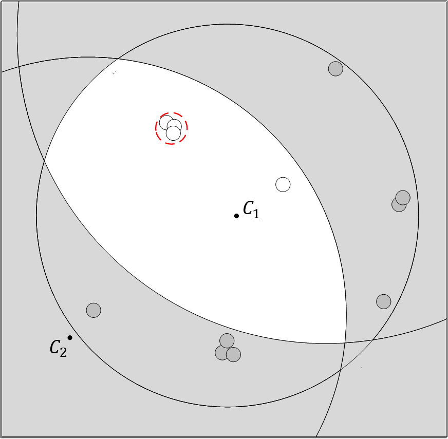
Figure 8. To search candidate locations based on a variant of CBG

Figure 8 illustrates the process. Formally, for each probe $P_{i}$, we draw a constraint circle centered at the probe, with the estimated distance between the probe and the target as the radius. Let $\{C_{1},C_{2},...,C_{i},...,C_{n}\}$ be the set of circles ordered in ascending order of radius $r_{i}$. We first query the organization name in $C_{1}$ by a map service (e.g. Google Map) and get a set of candidate coordinates (small circles in Figure 8). Some of them also fall into $C_{2}$, but the others do not. In the next loop, we remove those coordinates located outside of $C_{2}$. Similar logic can be applied to the rest loops. In the end, Several coordinates are left in the overlap region (the white region in Figure 8), called candidate coordinates. As shown by the red dashed circle, For adjacent coordinates with less than 1 km distance to each other, we merge them into one coordinate. If there is only one candidate coordinate left in the overlap region, we will map it to the target IP directly. If more than one, we use the coordinate selection algorithm (Section 2.2) to select the most possible location.

To estimate the radius of a constraint circle, we first use ping to measure the target IP and then convert the delay between each probe and the target device into a geographical distance by Formula 18. Percacci et al.(Percacci and Vespignani, 2003) has shown that packets travel in fiber optic cables at 2/3 the speed of light in a vacuum (denoted by c) . However, other literature(Gueye et al., 2006b)(Katz-Bassett et al., 2006) has demonstrated that 2/3 is a loose upper bound of converting factor because it does not take into account the transmission delay, the queuing delay, and the processing delay. Katz-Bassett et al.(Katz-Bassett et al., 2006) claims 4/9 is a safe threshold for constrains, so we adopt 4/9 as the converting factor $f$. Proved by Wang et al.(Wang et al., 2011a), by using this converting factor, the overlap region can always cover the targeted IP.

(18) $$r_{i}=\frac{p_{i}}{2}\cdot f\cdot c$$

Appendix C Organization dictionary

In most cases, LSTM-Ada works well for extracting organization name from copyright information due to the obvious patterns. Nevertheless, for some copyright information with an unconventional format, the model often fails to extract the correct or entire organization name. Besides, for organization names in the page title or the anchor text of logo images, the model also does not work due to the lack of context or regularity. Hence, we build an organization name dictionary to help extract the organization names.

Through crawling organization information from yellow pages and collecting POIs through Google Map API, we got the relevant information of 11,310,932 organizations, which contains their names. After removing duplicates, we got 7,757,970 organization names totally. These names are indexed with the first word as the key and the names under the same key are sorted in descending order of the length. With the dictionary, we extract organization from page text following three steps: 1) traverse every word $w_{i}$ in the text, and take the word $w_{i}$ as the key to look up the organization names which start with it. 2) traverse every organization name $o_{i}$ in the returned list, from the start word $w_{i}$, truncate the word sequence $s$ in the text with the same length as the current organization name $o_{i}$. 3) if the word sequence $s$ equals the organization name $o_{i}$, we return it as a result. Figure 9 shows an example of the extracting process.

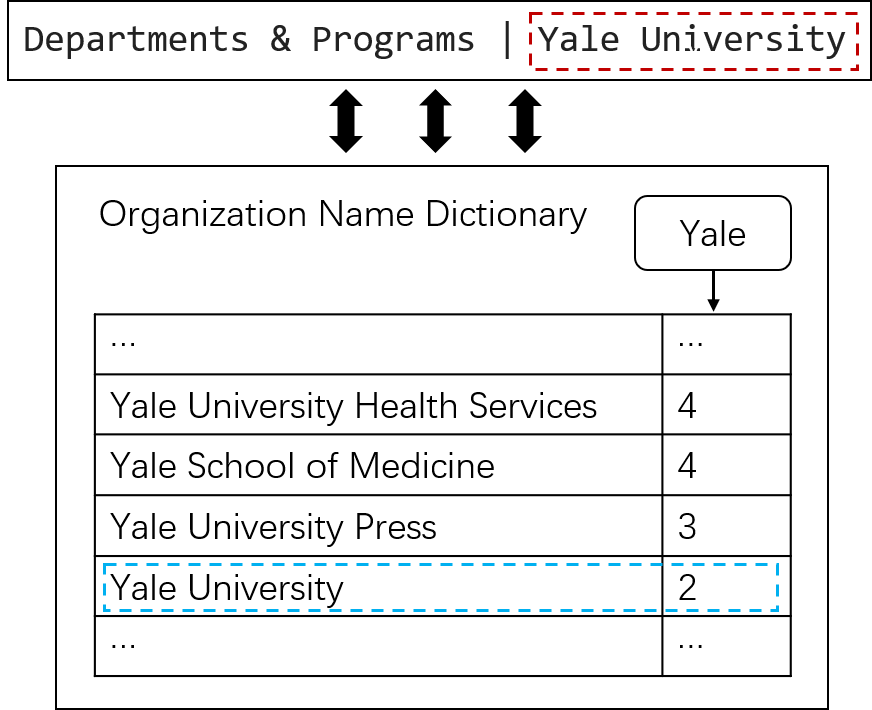
Figure 9. An example of extracting organization name by dictionary

Appendix D Open data

Datasets used in experiments, including WPLICE, PlanetLab-104, WebPages-8M, and RIPE-Atlas-1156 are open to the public for research. Visit https://github.com/131250208/dataset4XLBoost-Geo to download.