A Distributed Training Algorithm of Generative Adversarial Networks with Quantized Gradients

Abstract

Training generative adversarial networks (GAN) in a distributed fashion is a promising technology since it is contributed to training GAN on a massive of data efficiently in real-world applications. However, GAN is known to be difficult to train by SGD-type methods (may fail to converge) and the distributed SGD-type methods may also suffer from massive amount of communication cost. In this paper, we propose a distributed GANs training algorithm with quantized gradient, dubbed DQGAN, which is the first distributed training method with quantized gradient for GANs. The new method trains GANs based on a specific single machine algorithm called Optimistic Mirror Descent (OMD) algorithm, and is applicable to any gradient compression method that satisfies a general $\delta$-approximate compressor. The error-feedback operation we designed is used to compensate for the bias caused by the compression, and moreover, ensure the convergence of the new method. Theoretically, we establish the non-asymptotic convergence of DQGAN algorithm to first-order stationary point, which shows that the proposed algorithm can achieve a linear speedup in the parameter server model. Empirically, our experiments show that our DQGAN algorithm can reduce the communication cost and save the training time with slight performance degradation on both synthetic and real datasets.

1 Introduction

Generative adversarial networks (GANs)  [11], a kind of deep generative model, are designed to approximate the probability distribution of a massive of data. It has been demonstrated powerful for various tasks including images generation [35], video generation [45], and natural language processing [20], due to its ability to handle complex density functions. GANs are known to be notoriously difficult to train since they are non-convex non-concave min-max problems. Gradient descent-type algorithms are usually used for training generative adversarial networks, such as Adagrad [9], Adadelta [49], RMSprop [44] and Adam [15]. However, it recently has been demonstrated that gradient descent type algorithms are mainly designed for minimization problems and may fail to converge when dealing with min-max problems [23]. In addition, the learning rates of gradient type algorithms are hard to tune when they are applied to train GANs due to the absence of universal evaluation criteria like loss increasing or decreasing. Another critical problem for training GANs is that they usually contain a large number of parameters, thus may cost days or even weeks to train.

During the past years, much effort has been devoted for solving the above problems. Some recent works show that the Optimistic Mirror Descent (OMD) algorithm has superior performance for the min-max problems [23, 7, 10], which introduces an extra-gradient step to overcome the the divergence issue of gradient descent-type algorithms for solving the min-max problems. Recently, Daskalakis et al. [7] used OMD for training GAN in single machine. In addition, a few work also develop the distributed extragradient descent type algorithms to accelerate the training process of GANs [13, 19, 40, 43]. Recently, Liu et al. [21] have proposed distributed extragradient methods to train GANs with the decentralized network topology, but their method suffers from the large amount of parameters exchange problem since they did not compress the transmitted gradients.

In this paper, we propose a novel distributed training method for GANs, named as the Distributed Quantized Generative Adversarial Networks (DQGAN). The new method is able to accelerate the training process of GAN in distributed environment and a quantization technique is used to reduce the communication cost. To the best of our knowledge, this is the first distributed training method for GANs with quantization. The main contributions of this paper are summarized as three-fold:

• We have proposed a distributed optimization algorithm for training GANs. Our main novelty is that the gradient of communication is quantified, so that our algorithm has a smaller communication overhead to further improve the training speed. Through the error compensation operation we designed, we can solve the convergence problem caused by the quantization gradient.

• We have proved that the new method converges to first-order stationary point with non-asymptotic convergence under some common assumptions. The results of our analysis indicate that our proposed method can achieves a linear speedup in parameter server model.

• We have conducted experiments to demonstrate the effectiveness and efficiency of our proposed method on both synthesized and real datasets. The experimental results verify the convergence of the new method and show that our method is able to improve the speedup of distributed training with comparable performance with the state-of-the-art methods.

The rest of the paper is organized as follows. Related works and preliminaries are summarized in Section 2. The detailed DQGAN and its convergence rate are described in Section 3. The experimental results on both synthetic and real datasets are presented in Section 4. Conclusions are given in Section 5.

2 Notations and Related Work

In this section, we summarize the notations and definitions used in this paper, and give a brief review of related work.

2.1 Generative Adversarial Networks

Generative adversarial networks (GANs) consists of two components, one of which is a discriminator ($D$) distinguishing between real data and generated data while the other one is a generator ($G$) generating data to fool the discriminator. We define $p_{r}$ as the real data distribution and $p_{n}$ as the noise probability distribution of the generator $G$. The objective of a GAN is to make the generation data distribution of generator approximates the real data distribution $p_{r}$, which is formulated as a joint loss function for $D$ and $G$ [11]

$$\min_{\theta\in\Theta}\max_{\phi\in\Phi}\mathcal{L}\left(\theta,\phi\right),$$ (1)

where $\mathcal{L}\left(\theta,\phi\right)$ is defined as follows

$$\mathcal{L}\left(\theta,\phi\right)\overset{\text{def}}{=}\mathbb{E}_{\mathbf{x}\sim p_{r}}\left[\log D_{\phi}\left(\mathbf{x}\right)\right]+\mathbb{E}_{\mathbf{z}\sim p_{g}}\left[\log\left(1-D_{\phi}(G_{\theta}(\mathbf{z}))\right)\right].$$ (2)

$D_{\phi}(\mathbf{x})$ indicate that the discriminator which outputs a probability of its input being a real sample. $\theta$ is the parameters of generator $G$ and $\phi$ is the parameters of discriminator $D$.

However, (1) may suffer from saturating problem at the early learning stage and leads to vanishing gradients for the generator and inability to train in a stable manner [11, 2]. Then we used the loss in WGAN [11, 2]

$$\mathcal{L}\left(\theta,\phi\right)\overset{\text{def}}{=} \mathbb{E}_{\mathbf{x}\sim p_{r}}\left[D_{\phi}\left(\mathbf{x}\right)\right]-\mathbb{E}_{\mathbf{z}\sim p_{g}}\left[D_{\phi}(G_{\theta}(\mathbf{z}))\right].$$ (3)

Then training GAN turns into finding the following Nash equilibrium

$$\theta^{*}\in\mathop{\arg\min}_{\theta\in\Theta}\mathcal{L}_{G}\left(\theta,\phi^{*}\right),$$ (4)

$$\phi^{*}\in\mathop{\arg\min}_{\phi\in\Phi}\mathcal{L}_{D}\left(\theta^{*},\phi\right),$$ (5)

where

$$\mathcal{L}_{G}\left(\theta,\phi\right)\overset{\text{def}}{=}-\mathbb{E}_{\mathbf{z}\sim p_{n}}\left[D_{\phi}(G_{\theta}(\mathbf{z}))\right],$$ (6)

$$\mathcal{L}_{D}\left(\theta,\phi\right)\overset{\text{def}}{=}-\mathbb{E}_{\mathbf{x}\sim p_{r}}\left[D_{\phi}\left(\mathbf{x}\right)\right]+\mathbb{E}_{\mathbf{z}\sim p_{n}}\left[D_{\phi}(G_{\theta}(\mathbf{z})\right].$$ (7)

Gidel et al. [10] defines a stationary point as a couple $(\theta^{*},\phi^{*})$ such that the directional derivatives of both $\mathcal{L}_{G}\left(\theta,\phi^{*}\right)$ and $\mathcal{L}_{D}\left(\theta^{*},\phi\right)$ are non-negative, i.e.,

$$\nabla_{\theta}\mathcal{L}_{G}\left(\theta^{*},\phi^{*}\right)^{T}\left(\theta-\theta^{*}\right)\geq 0,~{}\forall(\theta,\phi)\in\Theta\times\Phi;$$ (8)

$$\nabla_{\phi}\mathcal{L}_{D}\left(\theta^{*},\phi^{*}\right)^{T}\left(\phi-\phi^{*}\right)\geq 0,~{}\forall(\theta,\phi)\in\Theta\times\Phi,$$ (9)

which can be compactly formulated as

$$F\left(\mathbf{w}^{*}\right)^{T} \left(\mathbf{w}-\mathbf{w}^{*}\right)\geq 0,~{}\forall\mathbf{w}\in\Omega,$$ (10)

where $\mathbf{w}\overset{\text{def}}{=}\left[\theta,~{}\phi\right]^{T}$, $\mathbf{w}^{*}\overset{\text{def}}{=}\left[\theta^{*},~{}\phi^{*}\right]^{T}$, $\Omega\overset{\text{def}}{=}\Theta\times\Phi$ and $F\left(\mathbf{w}\right)\overset{\text{def}}{=}\left[\nabla_{\theta}\mathcal{L}_{G}\left(\theta,\phi\right),~{}\nabla_{\phi}\mathcal{L}_{D}\left(\theta,\phi\right)\right]^{T}$.

Many works have been done for GAN. For example, some focus on the loss design, such as WGAN [2], SN-GAN [25], LS-GAN [33]; while the others focus on the network architecture design, such as CGAN [24], DCGAN [35], SAGAN [50]. However, only a few works focus on the distributed training of GAN [21], which is our focus.

2.2 Optimistic Mirror Descent

The update scheme of the basic gradient method is given by

$$\mathbf{w}_{t+1}=P_{w}\left[\mathbf{w}_{t}-\eta_{t}F(\mathbf{w}_{t})\right],$$ (11)

where $F(\mathbf{w}_{t})$ is the gradient at $\mathbf{w}_{t}$, $P_{w}\left[\cdot\right]$ is the projection onto the constraint set $w$ (if constraints are present) and $\eta_{t}$ is the step-size. The gradient descent algorithm is mainly designed for minimization problems and it was proved to be able to converge linearly under the strong monotonicity assumption on the operator $F(\mathbf{w}_{t})$ [4]. However, the basic gradient descent algorithm may produce a sequence that drifts away and cycles without converging when dealing with some special min-max problems [2], such as bi-linear objective in [23].

To solve the above problem, a practical approach is to compute the average of multiple iterates, which converges with a $O(\frac{1}{\sqrt{t}})$ rate [28]. Recently, the extragradient method [30] has been used for the min-max problems, due to its superior convergence rate of $O(\frac{1}{t})$. The idea of the extragradient can be traced back to Korpelevich [16] and Nemirovski [29]. The basic idea of the extragradient is to compute a lookahead gradient to guide the following step. The iterates of the extragradient are given by

$$\mathbf{w}_{t+\frac{1}{2}}=P_{w}\left[\mathbf{w}_{t}-\eta_{t}F(\mathbf{w}_{t})\right],$$ (12)

$$\mathbf{w}_{t+1}=P_{w}\left[\mathbf{w}_{t}-\eta_{t}F(\mathbf{w}_{t+\frac{1}{2}})\right].$$ (13)

However, we need to compute the gradient at both $\mathbf{w}_{t}$ and $\mathbf{w}_{t+\frac{1}{2}}$ in the above iterates. Chiang et al. [5] suggested to use the following iterates

$$\mathbf{w}_{t+\frac{1}{2}}=P_{w}\left[\mathbf{w}_{t}-\eta_{t}F(\mathbf{w}_{t-\frac{1}{2}})\right],$$ (14)

$$\mathbf{w}_{t+1}=P_{w}\left[\mathbf{w}_{t}-\eta_{t}F(\mathbf{w}_{t+\frac{1}{2}})\right],$$ (15)

in which we only need to the compute the gradient at $\mathbf{w}_{t+\frac{1}{2}}$ and reuse the gradient $F(\mathbf{w}_{t-\frac{1}{2}})$ computed in the last iteration.

Considering the unconstrained problem without projection, (14) and (15) reduce to

$$\mathbf{w}_{t+\frac{1}{2}}=\mathbf{w}_{t}-\eta_{t}F(\mathbf{w}_{t-\frac{1}{2}}),$$ (16)

$$\mathbf{w}_{t+1}=\mathbf{w}_{t}-\eta_{t}F(\mathbf{w}_{t+\frac{1}{2}}),$$ (17)

and it is easy to see that this update is equivalent to the following one line update as in  [7]

$$\mathbf{w}_{t+\frac{1}{2}}=\mathbf{w}_{t-\frac{1}{2}}-2\eta_{t}F(\mathbf{w}_{t-\frac{1}{2}})+\eta_{t}F(\mathbf{w}_{t-\frac{3}{2}}).$$ (18)

The optimistic mirror descent algorithm is shown Algorithm 1. To compute $\mathbf{w}_{t+1}$, it first generates an intermediate state $\mathbf{w}_{t+\frac{1}{2}}$ according to $\mathbf{w}_{t}$ and the gradient $F(\mathbf{w}_{t-\frac{1}{2}})$ computed in the last iteration, and then computes $\mathbf{w}_{t+1}$ according to both $\mathbf{w}_{t}$ and the gradient at $\mathbf{w}_{t+\frac{1}{2}}$. In the end of the iteration, $F(\mathbf{w}_{t+\frac{1}{2}})$ is stored for the next iteration. The optimistic mirror descent algorithm was used for online convex optimization [5] and by Rakhlin and general online learning [36]. Mertikopoulos et al. [23] used the optimistic mirror descent algorithm for training generative adversarial networks in single machine.

Algorithm 1 Optimistic Mirror Descent Algorithm

0:  step-size sequence $\eta_{t}>0$

1:  for $t=0,1,\ldots,T-1$ do

2:     retrieve $F\left(\mathbf{w}_{t-\frac{1}{2}}\right)$

3:     set $\mathbf{w}_{t+\frac{1}{2}}=\mathbf{w}_{t}-\eta_{t}F(\mathbf{w}_{t-\frac{1}{2}})$

4:     compute gradient $F\left(\mathbf{w}_{t+\frac{1}{2}}\right)$ at $\mathbf{w}_{t+\frac{1}{2}}$

5:     set $\mathbf{w}_{t+1}=P_{w}\left[\mathbf{w}_{t}-\eta_{t}F(\mathbf{w}_{t+\frac{1}{2}})\right]$

6:     store $F\left(\mathbf{w}_{t+\frac{1}{2}}\right)$

7:  end for

8:  Return $\mathbf{w}_{T}$

However, all of these works focus on the single machine setting and we will propose a training algorithm for distributed settings.

2.3 Distributed Training

Distributed centralized network and distributed decentralized network are two kinds of topologies used in distributed training.

In distributed centralized network topology, each worker node can obtain information of all other worker nodes. Centralized training systems have different implementations. There exist two common models in the distributed centralized network topology, i.e., the parameter server model [18] and the AllReduce model [34, 46]. The difference between the parameter server model and the AllReduce model is that each worker in the AllReduce model directly sends the gradient information to other workers without a server.

In the distributed decentralized network topology, the structure of computing nodes are usually organized into a graph to process and the network topology does not ensure that each worker node can obtain information of all other worker nodes. All worker nodes can only communicate with their neighbors. In this case, the network topology connection can be fixed or dynamically uncertain. Some parallel algorithms are designed for fixed topology [13, 19, 40, 43]. On the other hand, the network topology may change when the network accident or power accident causes the connection to be interrupted. Some method have been proposed for this kind of dynamic network topology [26, 27].

Recently, Liu et al. [21] proposed to train GAN with the decentralized network topology, but their method suffers from the large amount of parameters exchange problem since they did not compress the transmitted gradients. In this paper, we mainly focus on distributed training of GAN with the distributed centralized network topology.

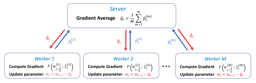
Figure 1: Distributed training of GAN in Algorithm 2 in parameter-server model.

2.4 Quantization

Quantization is a promising technique to reduce the neural network model size by reducing the number of bits of the parameters. Early studies on quantization focus on CNNs and RNNs. For example, Courbariaux et al. [6] proposed to use a single sign function with a scaling factor to binarize the weights and activations in the neural networks, Rastegari et al. [37] formulated the quantization as an optimization problem in order to quantize CNNs to a binary neural network, Zhou et al. [51] proposed to quantize the weights, activations and gradients. In the distributed training, the expensive communication cost can be reduced by quantizing the transmitted gradients.

Denote the quantization function as $Q(\mathbf{v})$ where $\mathbf{v}\in\mathbb{R}^{d}$. Generally speaking, existing gradient quantization techniques in distributed training can be divided into two categories, i.e., biased quantization ($\mathbb{E}[Q(\mathbf{v})]\neq\mathbf{v}$ for $\forall\mathbf{v}$) and unbiased quantization ($\mathbb{E}[Q(\mathbf{v})]=\mathbf{v}$ for any $\mathbf{v}$).

Biased gradient quantization: The sign function is a commonly-used biased quantization method [3, 39, 42]. Stich et al. [41] proposed a top-k quantization method which only retains the top $k$ largest elements of this vector and set the others to zero.

Unbiased gradient quantization: Such methods usually use stochastically quantized gradients [48, 1, 47]. For example, Alistarh et al. [1] proposed a compression operator which can be formulated as

$$Q(v_{i})=sign(v_{i})\cdot\|\mathbf{v}\|_{2}\cdot\xi_{i}(\mathbf{v},s),$$ (19)

where $\xi_{i}(\mathbf{v},s)$ is defined as follows

$$\xi_{i}(\mathbf{v},s)=\left\{\begin{aligned} &\frac{l}{s}&\text{with prob.}~{}1-\left(\frac{|v_{i}|}{\|\mathbf{v}\|_{2}}\cdot s-l\right);\\ &\frac{l+1}{s}&\text{otherwise}.\end{aligned},\right.$$ (20)

where $s$ is the number of quantization levels, $0\leq l<s$ is a integer such that $|v_{i}|/\|\mathbf{v}\|_{2}\in[l/s,(l+1)/s]$. Hou et al. [12] replaced the $\|\mathbf{v}\|_{2}$ in the above method with $\|\mathbf{v}\|_{\infty}$.

3 The Proposed Method

3.1 DQGAN Algorithm

Actually, we consider extensions of the algorithm to the context of a stochastic operator, i.e., we no longer have access to the exact gradient but to an unbiased stochastic estimate of it. Suppose we have $M$ machines. When in machine $m$ at $t$-th iteration, we sample a mini-batch according to $\xi_{t}^{(m)}=\left(\xi_{t,1}^{(m)},\xi_{t,2}^{(m)},\cdots,\xi_{t,B}^{(m)}\right)$, where $B$ is the minibatch size. In all $M$ machines, we use the same mini-batch size $B$. We use the term $F(\mathbf{w}_{t}^{(m)};\xi_{t,b}^{(m)})$   ($1\leq b\leq B$) and $F(\mathbf{w}_{t}^{(m)})$ to stand for stochastic gradient and gradient respectively. When in machine $m$ at $t$-th iteration, we define mini-batch gradient as $F(\mathbf{w}_{t}^{(m)};\xi_{t}^{(m)})=\frac{1}{B}\sum_{b=1}^{B}F(\mathbf{w}_{t}^{(m)};\xi_{t,b}^{(m)})$.

To reduce the size of the transmitted gradients in distributed training, we introduce a quantization function $Q(\cdot)$ to compress the gradients. In this paper, we consider a general $\delta$-approximate compressor for our method

Definition 1.

An quantization operator $Q$ is said to be $\delta$-approximate compressor for $\delta\in(0,1])$ if

$$\|Q\left(F(\mathbf{w})\right)-F(\mathbf{w})\|^{2}\leq(1-\delta)\|F(\mathbf{w})\|^{2}\quad\text{for all}~{}\mathbf{w}\in\Omega.$$ (21)

Before sending gradient data to the central server, each worker needs quantify the gradient data, which makes our algorithm have a small communication overhead. In addition, our algorithm is applicable to any gradient compression method that satisfies a general $\delta$-approximate compressor.

In general, the quantized gradient will lose some accuracy and cause the algorithm to fail to converge. In this paper, we have designed an error compensation operation to solve this problem, which is to incorporate the error made by the compression operator into the next step to compensate for gradients. Recently, Stich et al. [41] conducted the theoretical analysis of error-feedback in the strongly convex case and Karimireddy et al. [14] further extended the convergence results to the non-convex and weakly convex cases. These error-feedback operations are designed to solve the minimization problem. Here, in order to solve the min-max problem, we need to design the error-feedback operation more cleverly. In each iteration, we compensate the error caused by gradient quantization twice.

The proposed method, named as Distributed Quantized Generative Adversarial Networks (DQGAN), is summarized in Algorithm 2. The procedure of the new method is illustrated with the the parameter server model [18] in Figure 1. There are $M$ works participating in the model training. In this method, $\mathbf{w}_{0}$ is first initialized and pushed to all workers, and the local variable $\mathbf{e}^{m}_{0}$ is set to $0$ for $m\in[1,M]$.

In each iteration, the state $\mathbf{w}_{t-1}^{(m)}$ is updated to obtain the intermediate state $\mathbf{w}_{t-\frac{1}{2}}^{(m)}$ on $m$-th worker. Then each worker computes the gradients and adds the error compensation. The $m$-th worker computes the gradients $F(\mathbf{w}_{t-\frac{1}{2}}^{(m)};\xi_{t}^{(m)})$ and adds the error compensation $\mathbf{e}^{(m)}_{t-1}$ to obtain $\mathbf{p}_{t}^{(m)}$, and then quantizes it to $\hat{\mathbf{p}}_{t}^{(m)}$ and transmit the quantized one to the server. The error $\mathbf{e}_{t}^{(m)}$ is computed as the difference between $\mathbf{p}_{t}^{(m)}$ and $\hat{\mathbf{p}}_{t}^{(m)}$. The server will average all quantized gradients and push it to all workers. Then the new parameter $\mathbf{w}_{t}$ will be updated. Then we use it to update $\mathbf{w}_{t-1}$ to get the new parameter $\mathbf{w}_{t}$.

Algorithm 2 The Algorithm of DQGAN

0:  step-size $\eta>0$, Quantization function $Q\left(\cdot\right)$ is $\delta$-approximate compressor.

1:  Initialize $\mathbf{w}_{0}$ and push it to all workers, set $\mathbf{w}^{(m)}_{-\frac{1}{2}}=\mathbf{w}_{0}$ and $\mathbf{e}^{(m)}_{0}=0$ for $1\leq m\leq M$.

2:  for $t=1,2,\ldots,T$ do

3:     on worker m : $(m\in\{1,2,\cdots,M\})$

4:      set $\mathbf{w}_{t-\frac{1}{2}}^{(m)}=\mathbf{w}_{t-1}-\left[\eta F(\mathbf{w}_{t-\frac{3}{2}}^{(m)};\xi_{t-1}^{(m)})+\mathbf{e}^{(m)}_{t-1}\right]$

5:      compute gradient $F(\mathbf{w}_{t-\frac{1}{2}}^{(m)};\xi_{t}^{(m)})$

6:      set $\mathbf{p}_{t}^{(m)}=\eta F(\mathbf{w}_{t-\frac{1}{2}}^{(m)};\xi_{t}^{(m)})+\mathbf{e}^{(m)}_{t-1}$

7:      set $\hat{\mathbf{p}}_{t}^{(m)}=Q\left(\mathbf{p}_{t}^{(m)}\right)$ and push it to the server

8:      set $\mathbf{e}_{t}^{(m)}=\mathbf{p}_{t}^{(m)}-\hat{\mathbf{p}}_{t}^{(m)}$

9:     on server:

10:      pull $\hat{\mathbf{p}}_{t}^{(m)}$ from each worker

11:      set $\hat{\mathbf{q}}_{t}=\frac{1}{M}\left[\sum_{m=1}^{M}\hat{\mathbf{p}}_{t}^{(m)}\right]$

12:      push $\hat{\mathbf{q}}_{t}$ to each worker

13:     on worker m : $(m\in\{1,2,\cdots,M\})$

14:      set $\mathbf{w}_{t}=\mathbf{w}_{t-1}-\hat{\mathbf{q}}_{t}$

15:  end for

16:  Return $\mathbf{w}_{T}$

3.2 Coding Strategy

The quantization plays an important role in our method. In this paper, we proposed a general $\delta$-approximate compressor in order to include a variety of quantization methods for our method. In this subsection, we will prove that some commonly-used quantization methods are $\delta$-approximate compressors.

According to the definition of the $k$-contraction operator [41], we can verify the following theorem

Theorem 1.

The $k$-contraction operator [41] is a $\delta$-approximate compressor with $\delta=\frac{k}{d}$ where $d$ is the dimensions of input and $k\in(0,d]$ is a parameter.

Moreover, we can prove the following theorem

Theorem 2.

The quantization methods in [1] and [12] are $\delta$-approximate compressors.

Therefore, a variety of quantization methods can be used for our method.

3.3 Convergence Analysis

Throughout the paper, we make the following assumption

Assumption 1 (Lipschitz Continuous).

1. $F$ is $L$-Lipschitz continuous, i.e. $\|F(\mathbf{w}_{1})-F(\mathbf{w}_{2})\|\leq L\|\mathbf{w}_{1}-\mathbf{w}_{2}\|$ for $\forall\mathbf{w}_{1},\mathbf{w}_{2}$ .

2. $\|F(\mathbf{w})\|\leq G$ for $\forall\mathbf{w}$ .

Assumption 2 (Unbiased and Bounded Variance).

For $\forall\mathbf{w}_{t-\frac{1}{2}}^{(m)}$, we have $\mathbb{E}\left[F(\mathbf{w}_{t-\frac{1}{2}}^{(m)};\xi_{t,b}^{(m)})\right]=F(\mathbf{w}_{t-\frac{1}{2}}^{(m)})$ and $\mathbb{E}\|F(\mathbf{w}_{t-\frac{1}{2}}^{(m)};\xi_{t,b}^{(m)})-F(\mathbf{w}_{t-\frac{1}{2}}^{(m)})\|^{2}\leq\sigma^{2}$ , where $1\leq b\leq B$.

Assumption 3 (Pseudomonotonicity).

The operator $F$ is pseudomonotone, i.e.,

$$\left\langle F(\mathbf{w}_{2}),\mathbf{w}_{1}-\mathbf{w}_{2}\right\rangle\geq 0\Rightarrow\left\langle F(\mathbf{w}_{1}),\mathbf{w}_{1}-\mathbf{w}_{2}\right\rangle\geq 0\quad\text{for}\quad\forall\mathbf{w}_{1},\mathbf{w}_{2}$$

Now, we give a key Lemma, which shows that the residual errors maintained in Algorithm 2 do not accumulate too much.

Lemma 1.

At any iteration $t$ of Algorithm 2, the norm of the error $\frac{1}{M}\sum_{m=1}^{M}\|\mathbf{e}_{t}^{(m)}\|^{2}$ is bounded:

$$\mathbb{E}\left[\|\frac{1}{M}\sum_{m=1}^{M}\mathbf{e}^{(m)}_{t}\|^{2}\right]\leq\frac{8\eta^{2}(1-\delta)(G^{2}+\frac{\sigma^{2}}{B})}{\delta^{2}}$$ (22)

If $\delta=1$, then $\|\mathbf{e}_{t}^{(m)}\|=0$ for $1\leq m\leq M$ and the error is zero as expected.

Finally, based on above assumptions and lemma, we are on the position to describe the convergence rate of Algorithm 2.

Theorem 3.

By picking the $\eta\leq\min\{\frac{1}{\sqrt{BM}},\frac{1}{6\sqrt{2}L}\}$ in Algorithm 2, we have

$$\frac{1}{T}\sum_{t=1}^{T}\mathbb{E} \left[\|\frac{1}{M}\sum_{m=1}^{M}F\left(\mathbf{w}_{t-\frac{1}{2}}^{(m)};\xi_{t}^{(m)}\right)\|^{2}\right]\leq\frac{4\|\tilde{\mathbf{w}}_{0}-\mathbf{w}^{*}\|^{2}}{\eta^{2}T}+\frac{1728~{}L^{2}\sigma^{2}}{B^{2}M^{2}}$$ (23)

$$\quad+\frac{3456~{}L^{2}G^{2}(M-1)}{BM^{2}}+\frac{9216~{}L^{2}(1-\delta)(G^{2}+\frac{\sigma^{2}}{B})(M-1)}{\delta^{2}BM^{2}}+\frac{48~{}\sigma^{2}}{BM}$$

Theorem 23 gives such a non-asymptotic convergence and linear speedup in theory. We need to find the $\epsilon$-first-order stationary point, i.e.,

$$\mathbb{E}\left[\|\frac{1}{M}\sum_{m=1}^{M}F\left(\mathbf{w}_{t-\frac{1}{2}}^{(m)};\xi_{t}^{(m)}\right)\|^{2}\right]\leq\epsilon^{2}$$ (24)

By taking $M=\mathcal{O}(\epsilon^{-2})$ and $T=\mathcal{O}(\epsilon^{-8})$, we can guarantee that the algorithm 2 can reach an $\epsilon$-first-order stationary point.

4 Experiments

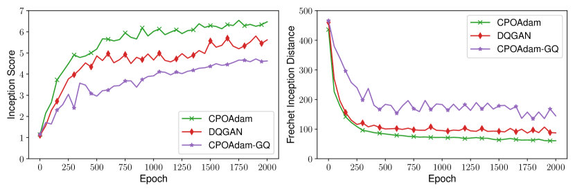
Figure 2: The Inception Score and Fréchet Inception Distance values of three methods on the CIFAR10 dataset.

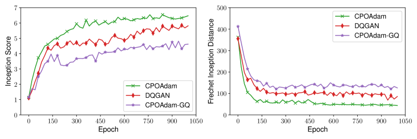
Figure 3: The Inception Score and Fréchet Inception Distance values of three methods on the CelebA dataset.

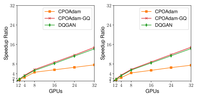
Figure 4: The speedup of our method on the CIFAR10 and CelebA datasets (left and right respectively).

In this section, we present the experimental results on real-life datasets. We used PyTorch [32] as the underlying deep learning framework and Nvidia NCCL [31] as the communication mechanism. We used the following two real-life benchmark datasets for the remaining experiments. The CIFAR-10 dataset [17] contains 60000 32x32 images in 10 classes: airplane, automobile, bird, cat, deer, dog, frog, horse, ship and truck. The CelebA dataset [22] is a large-scale face attributes dataset with more than 200K celebrity images, each with 40 attribute annotations.

We compared our method with the Centralized Parallel Optimistic Adam (CPOAdam) which is our method without quantization and error-feedback, and the Centralized Parallel Optimistic Adam with Gradients Quantization (CPOAdam-GQ) for training the generative adversarial networks with the loss in (3) and the deep convolutional generative adversarial network (DCGAN) architecture [35]. We implemented full-precision (float32) baseline models and set the number of bits for our method to $8$. We used the compressor in [12] for our method. Learning rates and hyperparameters in these methods were chosen by an inspection of grid search results so as to enable a fair comparison of these methods. We use the Inception Score [38] and fréchet inception distance [8] to evaluate all methods, where higher inception score and lower Fréchet Inception Distance indicate better results.

The Inception Score and Fréchet Inception Distance values of three methods on the CIFAR10 and CelebA datasets are shown in Figures 2 and 3. The results on both datasets show that the CPOAdam achieves high inception scores and lower fréchet inception distances with all epochs of training. We also notice that our method with 1/4 full precision gradients is able to produce comparable result with CPOAdam with full precision gradients, finally with at most $0.6$ decrease in terms of Inception Score and at most $30$ increase in terms of Fréchet Inception Distance on the CIFAR10 dataset, with at most $0.5$ decrease in terms of Inception Score and at most $40$ increase in terms of Fréchet Inception Distance on the CelebA dataset.

Finally, we show the speedup results of our method on the CIFAR10 and CelebA datasets in Figure 4, which shows that our method is able to improve the speedup of training GANs and the improvement becomes more significant with the increase of data size. With 32 workers, our method with $8$ bits of gradients achieves a significant improvement on the CIFAR10 and the CelebA dataset, compared to the CPOAdam. This is the same as our expectations, after all, 8bit transmits less data than 32bit.

5 Conclusion

In this paper, we have proposed a distributed optimization algorithm for training GANs. The new method reduces the communication cost via gradient compression, and the error-feedback operations we designed is used to compensate for the bias caused by the compression operation and ensure the non-asymptotic convergence. We have theoretically proved the non-asymptotic convergence of the new method, with the introduction of a general $\delta$-approximate compressor. Moreover, we have proved that the new method has linear speedup in theory. The experimental results show that our method is able to produce comparable results as the distributed OMD without quantization, only with slight performance degradation.

Although our new method has linear speedup in theory, the cost of gradients synchronization affects its performance in practice. Introducing gradient asynchronous communication technology will break the synchronization barrier and improve the efficiency of our method in real applications. We will leave this for the future work.

Appendix A The Proof of Theorem 1 and Theorem 2

According to the definition of the $k$-contraction operator , we can verify the Theorem 1.

Proof.

The $k$-contraction operator is a operator comp: $\mathbb{R}^{d}\rightarrow\mathbb{R}^{d}$ that satisfies the contraction property

$$\mathbb{E}\|\mathbf{v}-\text{comp}(\mathbf{v})\|^{2}\leq\left(1-\frac{k}{d}\right)\|\mathbf{v}\|^{2}~{}\forall\mathbf{v}\in\mathbb{R}^{d},$$ (25)

where $k$ is a parameter that satisfies $0<k\leq d$.

We set $\delta=\frac{k}{d}$. Then we have $\delta\in(0,1]$. Obviously, the $k$-contraction operator is a $\delta$-approximate compressor with $\delta=\frac{k}{d}$. ∎

For example, we can directly take the largest $k~{}(0<k\leq d)$ elements of $d$ elements in $\mathbf{v}$ in practice.

Moreover, we can prove the Theorem 2.

Proof.

The $m$-bit stochastic quantification method is defined as

$$Q(v_{i})=s\cdot\text{sign}(v_{i})\cdot q(v_{i},s),$$ (26)

where $v_{i}$ is the $i$-th element of vector $\mathbf{v}$, $s$ is a scalar and equals $\|\mathbf{v}\|_{2}$ or $\|\mathbf{v}\|_{\infty}$ , $q(v_{i},s)\in\{-B_{k},\cdots,-B_{1},B_{0},B_{1},\cdots,B_{k}\}$ and $0=B_{0}<B_{1}<\cdots<B_{k}$, $k=2^{m-1}-1$ denotes the number of quantized values that $m$-bit can represent. $q(v_{i},s)$ is defined as

$$q(v_{i},s)=\left\{\begin{aligned} &B_{r+1}&\text{with prob.}~{}\frac{\frac{|v_{i}|}{s}-B_{r}}{B_{r+1}-B_{r}};\\ &B_{r}&\text{otherwise}.\end{aligned},\right.$$ (27)

where $r\in\{0,1,\cdots,k-1\}$ satisfies $B_{r}\leq\frac{|v_{i}|}{s}<B_{r+1}$.

So we have

$$\mathbb{E}\left[Q(v_{i})\right]=s\cdot\text{sign}(v_{i})\cdot\left(B_{r+1}\cdot\frac{\frac{|v_{i}|}{s}-B_{r}}{B_{r+1}-B_{r}}+B_{r}\cdot\frac{B_{r+1}-\frac{|v_{i}|}{s}}{B_{r+1}-B_{r}}\right)=v_{i}$$ (28)

Note that $Q(\mathbf{v})$ is an unbiased estimator of $\mathbf{v}$.

To prove that the quantization methods are $\delta$-approximate compressors, i.e.,

$$\mathbb{E}\left[\|Q(\mathbf{v})-\mathbf{v}\|^{2}\right]\leq(1-\delta)\|\mathbf{v}\|^{2},$$ (29)

we just need to prove that for all element in $\mathbf{v}$, $Q(\cdot)$ satisfies

$$\mathbb{E}\left[|Q(v_{i})-v_{i}|^{2}\right]\leq(1-\delta)|v_{i}|^{2},$$ (30)

where $v_{i}$ is the $i$-th element of vector $\mathbf{v}$. When $v_{i}=0$, $Q(v_{i})=0$ and formula (30) holds. So our analysis below only considers the case of $v_{i}\neq 0$.

Since

$$\mathbb{E}\left[\|Q(v_{i})\|^{2}\right] =s^{2}\cdot\left(B_{r+1}^{2}\cdot\frac{\frac{|v_{i}|}{s}-B_{r}}{B_{r+1}-B_{r}}+B_{r}^{2}\cdot\frac{B_{r+1}-\frac{|v_{i}|}{s}}{B_{r+1}-B_{r}}\right)$$ (31)

$$=s^{2}\cdot\frac{\frac{|v_{i}|}{s}\left(B_{r+1}^{2}-B_{r}^{2}\right)-B_{r}B_{r+1}\left(B_{r+1}-B_{r}\right)}{B_{r+1}-B_{r}}$$

$$=|v_{i}|\cdot s\cdot\left(B_{r+1}+B_{r}\right)-B_{r}B_{r+1}\cdot s^{2}$$

and $\mathbb{E}\left[|Q(v_{i})-v_{i}|^{2}\right]=\mathbb{E}\left[|Q(v_{i})|^{2}\right]-|v_{i}|^{2}$ , the goal we need to prove is changed to

$$|v_{i}|\cdot s\cdot\left(B_{r+1}+B_{r}\right)-B_{r}B_{r+1}\cdot s^{2}\leq(2-\delta)|v_{i}|^{2}.$$ (32)

We set that $C_{r}=s\cdot B_{r}$, $C_{r+1}=s\cdot B_{r+1}$ and $a=|v_{i}|$ satisfies $C_{r}\leq a<C_{r+1}$.

Now, our goal is that we can find $\delta\in(0,1]$ satisfying

$$(2-\delta)\cdot a^{2}-\left(C_{r}+C_{r+1}\right)\cdot a+C_{r}C_{r+1}\geq 0\quad\forall~{}C_{r}\leq a<C_{r+1}.$$ (33)

This is easy to prove and we provide a proof method below.

After rearranging (33), there is

$$\delta\leq 2-\frac{\left(C_{r}+C_{r+1}\right)\cdot a-C_{r}C_{r+1}}{a^{2}}\quad\forall~{}C_{r}\leq a<C_{r+1}.$$ (34)

So, we just need to prove that

$$0<2-\frac{\left(C_{r}+C_{r+1}\right)\cdot a-C_{r}C_{r+1}}{a^{2}}\leq 1\quad\forall~{}C_{r}\leq a<C_{r+1}.$$ (35)

As long as (35) holds, $\delta$ that satisfies $\delta\in(0,1]$ exists.

First, we prove that

$$2-\frac{\left(C_{r}+C_{r+1}\right)\cdot a-C_{r}C_{r+1}}{a^{2}}>0\quad\forall~{}C_{r}\leq a<C_{r+1}.$$ (36)

That is

$$2a^{2}-\left(C_{r}+C_{r+1}\right)\cdot a+C_{r}C_{r+1}>0\quad\forall~{}C_{r}\leq a<C_{r+1}.$$ (37)

For this one-variable quadratic inequality, we just prove

$$\frac{C_{r}+C_{r+1}+\sqrt{\left(C_{r}+C_{r+1}\right)^{2}-8C_{r}C_{r+1}}}{4}<C_{r}.$$ (38)

(38) obviously holds after rearranging as follows.

$$\sqrt{\left(C_{r}+C_{r+1}\right)^{2}-8C_{r}C_{r+1}}<3C_{r}-C_{r+1}.$$ (39)

Second, we prove that

$$2-\frac{\left(C_{r}+C_{r+1}\right)\cdot a-C_{r}C_{r+1}}{a^{2}}\leq 1\quad\forall~{}C_{r}\leq a<C_{r+1}.$$ (40)

That is

$$a^{2}-\left(C_{r}+C_{r+1}\right)\cdot a+C_{r}C_{r+1}\leq 0\quad\forall~{}C_{r}\leq a<C_{r+1}.$$ (41)

After rearranging,

$$\left(a-C_{r}\right)\left(a-C_{r+1}\right)\leq 0\quad\forall~{}C_{r}\leq a<C_{r+1}.$$ (42)

(42) obviously holds. So far, theorem 2 has been proved. ∎

Appendix B Proof of Lemma and Theorem

B.1 Proof of Lemma 1

Proof.

By definition of the error sequence,

$$\|\mathbf{e}^{(m)}_{t}\|^{2}=\|\mathbf{p}^{(m)}_{t}-Q(\mathbf{p}^{(m)}_{t})\|^{2}\leq(1-\delta)\|\mathbf{p}^{(m)}_{t}\|^{2}$$ (43)

$$=(1-\delta)\|\eta F(\mathbf{w}_{t-\frac{1}{2}}^{(m)};\xi_{t}^{(m)})+\mathbf{e}^{(m)}_{t-1}\|^{2}$$

$$=(1-\delta)\|\mathbf{e}^{(m)}_{t-1}\|^{2}+(1-\delta)\eta^{2}\|F(\mathbf{w}_{t-\frac{1}{2}}^{(m)};\xi_{t}^{(m)})\|^{2}+(1-\delta)\left\langle\eta F(\mathbf{w}_{t-\frac{1}{2}}^{(m)};\xi_{t}^{(m)}),\mathbf{e}^{(m)}_{t-1}\right\rangle$$

$$\leq(1-\delta)\left(1+K_{1}\right)\|\mathbf{e}^{(m)}_{t-1}\|^{2}+(1-\delta)\left(1+\frac{1}{K_{1}}\right)\eta^{2}\|F(\mathbf{w}_{t-\frac{1}{2}}^{(m)};\xi_{t}^{(m)})\|^{2}$$

In the last inequality, we use the Young’s inequality and $K_{1}>0$ is constant. So, we give the simple algebraic computations to solve the recurrence relation above:

$$\mathbb{E}\left[\|\mathbf{e}^{(m)}_{t}\|^{2}\right]$$ (44)

$$\leq(1-\delta)\left(1+K_{1}\right)\mathbb{E}\left[\|\mathbf{e}^{(m)}_{t-1}\|^{2}\right]+(1-\delta)\left(1+\frac{1}{K_{1}}\right)\cdot\mathbb{E}\left[\eta^{2}\|F(\mathbf{w}_{t-\frac{1}{2}}^{(m)};\xi_{t}^{(m)})\|^{2}\right]$$

$$\leq(1-\delta)\left(1+K_{1}\right)\mathbb{E}\left[\|\mathbf{e}^{(m)}_{t-1}\|^{2}\right]$$

$$\quad+(1-\delta)\left(1+\frac{1}{K_{1}}\right)\eta^{2}\cdot\mathbb{E}\left[2\|F(\mathbf{w}_{t-\frac{1}{2}}^{(m)})\|^{2}+2\|F(\mathbf{w}_{t-\frac{1}{2}}^{(m)})-F(\mathbf{w}_{t-\frac{1}{2}}^{(m)};\xi_{t}^{(m)})\|^{2}\right]$$

$$\leq\sum^{t}_{i=0}\left[(1-\delta)\left(1+K_{1}\right)\right]^{t-i}(1-\delta)\left(1+\frac{1}{K_{1}}\right)2\eta^{2}(G^{2}+\frac{\sigma^{2}}{B})$$

$$\leq\sum^{\infty}_{i=0}\left[(1-\delta)\left(1+K_{1}\right)\right]^{i}(1-\delta)\left(1+\frac{1}{K_{1}}\right)2\eta^{2}(G^{2}+\frac{\sigma^{2}}{B})$$

$$=\frac{(1-\delta)\left(1+\frac{1}{K_{1}}\right)}{1-\left[(1-\delta)\left(1+K_{1}\right)\right]}2\eta^{2}(G^{2}+\frac{\sigma^{2}}{B})$$

$$=\frac{(1-\delta)\left(1+\frac{1}{K_{1}}\right)}{\delta-K_{1}\left(1-\delta\right)}2\eta^{2}(G^{2}+\frac{\sigma^{2}}{B})$$

We take $K_{1}=\frac{\delta}{2(1-\delta)}$ such that $1+\frac{1}{K_{1}}=\frac{2-\delta}{\delta}\leq\frac{2}{\delta}$. Plugging this in the above gives

$$\mathbb{E}\left[\|\mathbf{e}^{(m)}_{t}\|^{2}\right] \leq\frac{(1-\delta)\left(1+\frac{1}{K_{1}}\right)}{\delta-K_{1}\left(1-\delta\right)}\cdot 2\eta^{2}(G^{2}+\frac{\sigma^{2}}{B})$$ (45)

$$=\frac{2(1-\delta)\left(1+\frac{1}{K_{1}}\right)}{\delta}\cdot 2\eta^{2}(G^{2}+\frac{\sigma^{2}}{B})$$

$$\leq\frac{8\eta^{2}(1-\delta)(G^{2}+\frac{\sigma^{2}}{B})}{\delta^{2}}$$

Then we have

$$\mathbb{E}\left[\|\frac{1}{M}\sum_{m=1}^{M}\mathbf{e}^{(m)}_{t}\|^{2}\right] =\mathbb{E}\left[\frac{1}{M^{2}}\|\sum_{m=1}^{M}\mathbf{e}^{(m)}_{t}\|^{2}\right]$$ (46)

$$\leq\mathbb{E}\left[\frac{1}{M^{2}}\cdot M\sum_{m=1}^{M}\|\mathbf{e}^{(m)}_{t}\|^{2}\right]$$

$$=\mathbb{E}\left[\frac{1}{M}\cdot\sum_{m=1}^{M}\|\mathbf{e}^{(m)}_{t}\|^{2}\right]$$

$$\leq\frac{8\eta^{2}(1-\delta)(G^{2}+\frac{\sigma^{2}}{B})}{\delta^{2}}.$$

In the first inequality, we used the Cauchy-Schwarz inequality. ∎

B.2 Main Proof of Theorem of 23

Proof.

Define $\bar{\mathbf{w}}_{t-\frac{1}{2}}=\frac{1}{M}\sum_{m=1}^{M}\mathbf{w}_{t-\frac{1}{2}}^{(m)}$, $\mathbf{\epsilon}_{t}^{(m)}=F\left(\mathbf{w}_{t-\frac{1}{2}}^{(m)};\xi_{t}^{(m)}\right)-F\left(\mathbf{w}_{t-\frac{1}{2}}^{(m)}\right)$ and $\bar{\mathbf{\epsilon}}_{t}=\frac{1}{M}\sum_{m=1}^{M}\mathbf{\epsilon}_{t}^{(m)}$ .

We consider the error-corrected sequence $\tilde{\mathbf{w}}_{t}$ which represents $\mathbf{w}_{t}$ with the delayed information added:

$$\tilde{\mathbf{w}}_{t}=\mathbf{w}_{t}-\frac{1}{M}\sum_{m=1}^{M}\mathbf{e}_{t}^{(m)}.$$ (47)

It satisfies the recurrence

$$\tilde{\mathbf{w}}_{t} =\mathbf{w}_{t}-\frac{1}{M}\sum_{m=1}^{M}\mathbf{e}_{t}^{(m)}$$ (48)

$$=\mathbf{w}_{t-1}-\frac{1}{M}\sum_{m=1}^{M}Q\left(\mathbf{p}_{t}^{(m)}\right)-\frac{1}{M}\sum_{m=1}^{M}\mathbf{e}_{t}^{(m)}$$

$$=\mathbf{w}_{t-1}-\frac{1}{M}\sum_{m=1}^{M}\mathbf{p}_{t}^{(m)}$$

$$=\mathbf{w}_{t-1}-\frac{1}{M}\sum_{m=1}^{M}\eta F\left(\mathbf{w}_{t-\frac{1}{2}}^{(m)};\xi_{t}^{(m)}\right)-\frac{1}{M}\sum_{m=1}^{M}\mathbf{e}_{t-1}^{(m)}$$

$$=\tilde{\mathbf{w}}_{t-1}-\frac{1}{M}\sum_{m=1}^{M}\eta F\left(\mathbf{w}_{t-\frac{1}{2}}^{(m)};\xi_{t}^{(m)}\right).$$

Suppose that $\mathbf{w}^{*}$ is an optimum solution.

$$\|\tilde{\mathbf{w}}_{t}-\mathbf{w}^{*}\|^{2}=\|\tilde{\mathbf{w}}_{t-1}-\frac{1}{M}\sum_{m=1}^{M}\eta F\left(\mathbf{w}_{t-\frac{1}{2}}^{(m)};\xi_{t}^{(m)}\right)-\mathbf{w}^{*}\|^{2}$$ (49)

$$=\|\tilde{\mathbf{w}}_{t-1}-\frac{1}{M}\sum_{m=1}^{M}\eta F\left(\mathbf{w}_{t-\frac{1}{2}}^{(m)};\xi_{t}^{(m)}\right)-\mathbf{w}^{*}\|^{2}$$

$$\quad\quad-\|\tilde{\mathbf{w}}_{t-1}-\frac{1}{M}\sum_{m=1}^{M}\eta F\left(\mathbf{w}_{t-\frac{1}{2}}^{(m)};\xi_{t}^{(m)}\right)-\tilde{\mathbf{w}}_{t}\|^{2}$$

$$=\|\tilde{\mathbf{w}}_{t-1}-\mathbf{w}^{*}\|^{2}-\|\tilde{\mathbf{w}}_{t-1}-\tilde{\mathbf{w}}_{t}\|^{2}+2\left\langle\mathbf{w}^{*}-\tilde{\mathbf{w}}_{t},\frac{1}{M}\sum_{m=1}^{M}\eta F\left(\mathbf{w}_{t-\frac{1}{2}}^{(m)};\xi_{t}^{(m)}\right)\right\rangle$$

$$=\|\tilde{\mathbf{w}}_{t-1}-\mathbf{w}^{*}\|^{2}-\|\tilde{\mathbf{w}}_{t-1}-\tilde{\mathbf{w}}_{t}\|^{2}+2\left\langle\mathbf{w}^{*}-\bar{\mathbf{w}}_{t-\frac{1}{2}},\frac{1}{M}\sum_{m=1}^{M}\eta F\left(\mathbf{w}_{t-\frac{1}{2}}^{(m)};\xi_{t}^{(m)}\right)\right\rangle$$

$$\quad\quad+2\left\langle\bar{\mathbf{w}}_{t-\frac{1}{2}}-\tilde{\mathbf{w}}_{t},\frac{1}{M}\sum_{m=1}^{M}\eta F\left(\mathbf{w}_{t-\frac{1}{2}}^{(m)};\xi_{t}^{(m)}\right)\right\rangle$$

$$=\|\tilde{\mathbf{w}}_{t-1}-\mathbf{w}^{*}\|^{2}-\|\tilde{\mathbf{w}}_{t-1}-\bar{\mathbf{w}}_{t-\frac{1}{2}}+\bar{\mathbf{w}}_{t-\frac{1}{2}}-\tilde{\mathbf{w}}_{t}\|^{2}$$

$$\quad\quad+2\left\langle\mathbf{w}^{*}-\bar{\mathbf{w}}_{t-\frac{1}{2}},\frac{1}{M}\sum_{m=1}^{M}\eta F\left(\mathbf{w}_{t-\frac{1}{2}}^{(m)};\xi_{t}^{(m)}\right)\right\rangle$$

$$\quad\quad+2\left\langle\bar{\mathbf{w}}_{t-\frac{1}{2}}-\tilde{\mathbf{w}}_{t},\frac{1}{M}\sum_{m=1}^{M}\eta F\left(\mathbf{w}_{t-\frac{1}{2}}^{(m)};\xi_{t}^{(m)}\right)\right\rangle$$

$$=\|\tilde{\mathbf{w}}_{t-1}-\mathbf{w}^{*}\|^{2}-\|\tilde{\mathbf{w}}_{t-1}-\bar{\mathbf{w}}_{t-\frac{1}{2}}\|^{2}-\|\bar{\mathbf{w}}_{t-\frac{1}{2}}-\tilde{\mathbf{w}}_{t}\|^{2}$$

$$\quad\quad+2\left\langle\mathbf{w}^{*}-\bar{\mathbf{w}}_{t-\frac{1}{2}},\frac{1}{M}\sum_{m=1}^{M}\eta F\left(\mathbf{w}_{t-\frac{1}{2}}^{(m)};\xi_{t}^{(m)}\right)\right\rangle$$

$$\quad\quad+2\left\langle\tilde{\mathbf{w}}_{t}-\bar{\mathbf{w}}_{t-\frac{1}{2}},\tilde{\mathbf{w}}_{t-1}-\bar{\mathbf{w}}_{t-\frac{1}{2}}-\frac{1}{M}\sum_{m=1}^{M}\eta F\left(\mathbf{w}_{t-\frac{1}{2}}^{(m)};\xi_{t}^{(m)}\right)\right\rangle$$

Note that

$$\mathbb{E}\left[2\left\langle\mathbf{w}^{*}-\bar{\mathbf{w}}_{t-\frac{1}{2}},\frac{1}{M}\sum_{m=1}^{M}\eta F\left(\mathbf{w}_{t-\frac{1}{2}}^{(m)};\xi_{t}^{(m)}\right)\right\rangle\right]$$ (50)

$$=\mathbb{E}\left[2\left\langle\mathbf{w}^{*}-\bar{\mathbf{w}}_{t-\frac{1}{2}},\frac{1}{M}\sum_{m=1}^{M}\eta F\left(\mathbf{w}_{t-\frac{1}{2}}^{(m)}\right)\right\rangle\right]$$

$$\quad\quad+\mathbb{E}\left[2\left\langle\mathbf{w}^{*}-\bar{\mathbf{w}}_{t-\frac{1}{2}},\frac{1}{M}\sum_{m=1}^{M}\eta F\left(\mathbf{w}_{t-\frac{1}{2}}^{(m)};\xi_{t}^{(m)}\right)-\frac{1}{M}\sum_{m=1}^{M}\eta F\left(\mathbf{w}_{t-\frac{1}{2}}^{(m)}\right)\right\rangle\right]$$

$$\overset{(a)}{\leq}\mathbb{E}\left[2\left\langle\mathbf{w}^{*}-\bar{\mathbf{w}}_{t-\frac{1}{2}},\frac{1}{M}\sum_{m=1}^{M}\eta F\left(\mathbf{w}_{t-\frac{1}{2}}^{(m)};\xi_{t}^{(m)}\right)-\frac{1}{M}\sum_{m=1}^{M}\eta F\left(\mathbf{w}_{t-\frac{1}{2}}^{(m)}\right)\right\rangle\right]\overset{(b)}{=}0$$

where $(a)$ holds by the pseudomonotonicity of operator $F$, $(b)$ hold since $\mathbb{E}\left[F(\mathbf{w}_{t-\frac{1}{2}}^{(m)};\xi_{t,b}^{(m)})\right]=F(\mathbf{w}_{t-\frac{1}{2}}^{(m)})$ ($1\leq b\leq B$). Since 48, we have

$$2\left\langle\tilde{\mathbf{w}}_{t}-\bar{\mathbf{w}}_{t-\frac{1}{2}},\tilde{\mathbf{w}}_{t-1}-\bar{\mathbf{w}}_{t-\frac{1}{2}}-\frac{1}{M}\sum_{m=1}^{M}\eta F\left(\mathbf{w}_{t-\frac{1}{2}}^{(m)};\xi_{t}^{(m)}\right)\right\rangle$$ (51)

$$=2\left\langle\tilde{\mathbf{w}}_{t}-\bar{\mathbf{w}}_{t-\frac{1}{2}},\tilde{\mathbf{w}}_{t}-\bar{\mathbf{w}}_{t-\frac{1}{2}}\right\rangle=2\|\tilde{\mathbf{w}}_{t}-\bar{\mathbf{w}}_{t-\frac{1}{2}}\|^{2}$$

$$=2\|\tilde{\mathbf{w}}_{t-1}-\bar{\mathbf{w}}_{t-\frac{1}{2}}-\frac{1}{M}\sum_{m=1}^{M}\eta F\left(\mathbf{w}_{t-\frac{1}{2}}^{(m)};\xi_{t}^{(m)}\right)\|^{2}$$

In addition, according to the update rules in Algorithm 2, we have

$$\bar{\mathbf{w}}_{t-\frac{1}{2}}=\mathbf{w}_{t-1}-\frac{1}{M}\sum_{m=1}^{M}\eta F\left(\mathbf{w}_{t-\frac{3}{2}}^{(m)};\xi_{t-1}^{(m)}\right)-\frac{1}{M}\sum_{m=1}^{M}\mathbf{e}_{t-1}^{(m)}$$ (52)

We combine 51 and 52, which yield

$$2\left\langle\tilde{\mathbf{w}}_{t}-\bar{\mathbf{w}}_{t-\frac{1}{2}},\tilde{\mathbf{w}}_{t-1}-\bar{\mathbf{w}}_{t-\frac{1}{2}}-\frac{1}{M}\sum_{m=1}^{M}\eta F\left(\mathbf{w}_{t-\frac{1}{2}}^{(m)};\xi_{t}^{(m)}\right)\right\rangle$$ (53)

$$=2\|\tilde{\mathbf{w}}_{t-1}-\left[\tilde{\mathbf{w}}_{t-1}-\frac{1}{M}\sum_{m=1}^{M}\eta F\left(\mathbf{w}_{t-\frac{3}{2}}^{(m)};\xi_{t-1}^{(m)}\right)\right]-\frac{1}{M}\sum_{m=1}^{M}\eta F\left(\mathbf{w}_{t-\frac{1}{2}}^{(m)};\xi_{t}^{(m)}\right)\|^{2}$$

$$=2\|\frac{1}{M}\sum_{m=1}^{M}\eta F\left(\mathbf{w}_{t-\frac{3}{2}}^{(m)};\xi_{t-1}^{(m)}\right)-\frac{1}{M}\sum_{m=1}^{M}\eta F\left(\mathbf{w}_{t-\frac{1}{2}}^{(m)};\xi_{t}^{(m)}\right)\|^{2}$$

$$\overset{(a)}{\leq}6\eta^{2}\|\frac{1}{M}\sum_{m=1}^{M}F\left(\mathbf{w}_{t-\frac{3}{2}}^{(m)}\right)-\frac{1}{M}\sum_{m=1}^{M}F\left(\mathbf{w}_{t-\frac{1}{2}}^{(m)}\right)\|^{2}+6\eta^{2}\|\bar{\mathbf{\epsilon}}_{t}\|^{2}+6\eta^{2}\|\bar{\mathbf{\epsilon}}_{t-1}\|^{2}$$

$$\overset{(b)}{\leq}18\eta^{2}\|\frac{1}{M}\sum_{m=1}^{M}F\left(\mathbf{w}_{t-\frac{3}{2}}^{(m)}\right)-F\left(\bar{\mathbf{w}}_{t-\frac{3}{2}}\right)\|^{2}+18\eta^{2}\|F\left(\bar{\mathbf{w}}_{t-\frac{3}{2}}\right)-F\left(\bar{\mathbf{w}}_{t-\frac{1}{2}}\right)\|^{2}$$

$$\quad\quad\quad\quad+18\eta^{2}\|F\left(\bar{\mathbf{w}}_{t-\frac{1}{2}}\right)-\frac{1}{M}\sum_{m=1}^{M}F\left(\mathbf{w}_{t-\frac{1}{2}}^{(m)}\right)\|^{2}+6\eta^{2}\|\bar{\mathbf{\epsilon}}_{t}\|^{2}+6\eta^{2}\|\bar{\mathbf{\epsilon}}_{t-1}\|^{2}$$

$$\overset{(c)}{\leq}18\eta^{2}\|\frac{1}{M}\sum_{m=1}^{M}F\left(\mathbf{w}_{t-\frac{3}{2}}^{(m)}\right)-F\left(\bar{\mathbf{w}}_{t-\frac{3}{2}}\right)\|^{2}+18\eta^{2}L^{2}\|\bar{\mathbf{w}}_{t-\frac{3}{2}}-\bar{\mathbf{w}}_{t-\frac{1}{2}}\|^{2}$$

$$\quad\quad\quad\quad+18\eta^{2}\|F\left(\bar{\mathbf{w}}_{t-\frac{1}{2}}\right)-\frac{1}{M}\sum_{m=1}^{M}F\left(\mathbf{w}_{t-\frac{1}{2}}^{(m)}\right)\|^{2}+6\eta^{2}\|\bar{\mathbf{\epsilon}}_{t}\|^{2}+6\eta^{2}\|\bar{\mathbf{\epsilon}}_{t-1}\|^{2}$$

$$\overset{(d)}{\leq}18\eta^{2}\|\frac{1}{M}\sum_{m=1}^{M}F\left(\mathbf{w}_{t-\frac{3}{2}}^{(m)}\right)-F\left(\bar{\mathbf{w}}_{t-\frac{3}{2}}\right)\|^{2}$$

$$\quad\quad\quad\quad+18\eta^{2}\|F\left(\bar{\mathbf{w}}_{t-\frac{1}{2}}\right)-\frac{1}{M}\sum_{m=1}^{M}F\left(\mathbf{w}_{t-\frac{1}{2}}^{(m)}\right)\|^{2}$$

$$\quad\quad\quad\quad+36\eta^{2}L^{2}\left(\|\bar{\mathbf{w}}_{t-\frac{3}{2}}-\tilde{\mathbf{w}}_{t-1}\|^{2}+\|\tilde{\mathbf{w}}_{t-1}-\bar{\mathbf{w}}_{t-\frac{1}{2}}\|^{2}\right)$$

$$\quad\quad\quad\quad+6\eta^{2}\|\bar{\mathbf{\epsilon}}_{t}\|^{2}+6\eta^{2}\|\bar{\mathbf{\epsilon}}_{t-1}\|^{2}$$

where $(a)$ and $(b)$ hold since $\|\mathbf{a}+\mathbf{b}+\mathbf{c}\|^{2}\leq 3\|\mathbf{a}\|^{2}+3\|\mathbf{b}\|^{2}+3\|\mathbf{c}\|^{2}$, $(c)$ holds by the $L$-Lipschitz continuity of $F$, $(d)$ holds since $\|\mathbf{a}+\mathbf{b}\|^{2}\leq 2\|\mathbf{a}\|^{2}+2\|\mathbf{b}\|^{2}$.

We combine (49), (50) and (53), which yield

$$\mathbb{E}\left[\|\tilde{\mathbf{w}}_{t}-\mathbf{w}^{*}\|^{2}\right]$$ (54)

$$\leq\mathbb{E}\left[\|\tilde{\mathbf{w}}_{t-1}-\mathbf{w}^{*}\|^{2}\right]-\mathbb{E}\left[\|\tilde{\mathbf{w}}_{t-1}-\bar{\mathbf{w}}_{t-\frac{1}{2}}\|^{2}\right]-\mathbb{E}\left[\|\bar{\mathbf{w}}_{t-\frac{1}{2}}-\tilde{\mathbf{w}}_{t}\|^{2}\right]$$

$$\quad+18\eta^{2}\mathbb{E}\left[\|\frac{1}{M}\sum_{m=1}^{M}F\left(\mathbf{w}_{t-\frac{3}{2}}^{(m)}\right)-F\left(\bar{\mathbf{w}}_{t-\frac{3}{2}}\right)\|^{2}\right]$$

$$\quad+18\eta^{2}\mathbb{E}\left[\|F\left(\bar{\mathbf{w}}_{t-\frac{1}{2}}\right)-\frac{1}{M}\sum_{m=1}^{M}F\left(\mathbf{w}_{t-\frac{1}{2}}^{(m)}\right)\|^{2}\right]$$

$$\quad+36\eta^{2}L^{2}\left(\mathbb{E}\left[\|\bar{\mathbf{w}}_{t-\frac{3}{2}}-\tilde{\mathbf{w}}_{t-1}\|^{2}\right]+\mathbb{E}\left[\|\tilde{\mathbf{w}}_{t-1}-\bar{\mathbf{w}}_{t-\frac{1}{2}}\|^{2}\right]\right)$$

$$\quad+6\eta^{2}\mathbb{E}\left[\|\bar{\mathbf{\epsilon}}_{t}\|^{2}\right]+6\eta^{2}\mathbb{E}\left[\|\bar{\mathbf{\epsilon}}_{t-1}\|^{2}\right]$$

Note that

$$\mathbb{E}\left[\|\frac{1}{M}\sum_{m=1}^{M}F\left(\mathbf{w}_{t-\frac{1}{2}}^{(m)}\right)-F\left(\bar{\mathbf{w}}_{t-\frac{1}{2}}\right)\|^{2}\right]\leq\frac{1}{M}\sum_{m=1}^{M}\mathbb{E}\left[\|F\left(\mathbf{w}_{t-\frac{1}{2}}^{(m)}\right)-F\left(\bar{\mathbf{w}}_{t-\frac{1}{2}}\right)\|^{2}\right]$$ (55)

$$\overset{(a)}{\leq}\frac{L^{2}}{M}\sum_{m=1}^{M}\mathbb{E}\left[\|\mathbf{w}_{t-\frac{1}{2}}^{(m)}-\bar{\mathbf{w}}_{t-\frac{1}{2}}\|^{2}\right]$$

$$\overset{(b)}{=}\frac{L^{2}}{M}\sum_{m=1}^{M}\mathbb{E}[\|\left(\mathbf{w}_{t-1}-\eta F\left(\mathbf{w}_{t-\frac{3}{2}}^{(m)};\xi_{t-1}^{(m)}\right)-\mathbf{e}_{t-1}^{(m)}\right)-(\mathbf{w}_{t-1}-$$

$$\quad\quad\quad\quad\frac{1}{M}\sum_{m^{{}^{\prime}}=1}^{M}\eta F\left(\mathbf{w}_{t-\frac{3}{2}}^{(m^{{}^{\prime}})};\xi_{t-1}^{(m^{{}^{\prime}})}\right)-\frac{1}{M}\sum_{m^{{}^{\prime}}=1}^{M}\mathbf{e}_{t-1}^{(m^{{}^{\prime}})})~{}\|^{2}]$$

$$=\frac{L^{2}}{M}\sum_{m=1}^{M}\mathbb{E}[\|\left(\frac{1}{M}\sum_{m^{{}^{\prime}}=1}^{M}\eta F\left(\mathbf{w}_{t-\frac{3}{2}}^{(m^{{}^{\prime}})};\xi_{t-1}^{(m^{{}^{\prime}})}\right)-\eta F\left(\mathbf{w}_{t-\frac{3}{2}}^{(m)};\xi_{t-1}^{(m)}\right)\right)$$

$$\quad\quad\quad\quad+\left(\frac{1}{M}\sum_{m^{{}^{\prime}}=1}^{M}\mathbf{e}_{t-1}^{(m^{{}^{\prime}})}-\mathbf{e}_{t-1}^{(m)}\right)\|^{2}]$$

$$\leq\frac{2L^{2}\eta^{2}}{M}\sum_{m=1}^{M}\mathbb{E}\left[\|\frac{1}{M}\sum_{m^{{}^{\prime}}=1}^{M}F\left(\mathbf{w}_{t-\frac{3}{2}}^{(m^{{}^{\prime}})};\xi_{t-1}^{(m^{{}^{\prime}})}\right)-F\left(\mathbf{w}_{t-\frac{3}{2}}^{(m)};\xi_{t-1}^{(m)}\right)\|^{2}\right]$$

$$\quad\quad\quad\quad+\frac{2L^{2}}{M}\sum_{m=1}^{M}\mathbb{E}\left[\|\frac{1}{M}\sum_{m^{{}^{\prime}}=1}^{M}\mathbf{e}_{t-1}^{(m^{{}^{\prime}})}-\mathbf{e}_{t-1}^{(m)}\|^{2}\right]$$

$$\overset{(c)}{\leq}\frac{6L^{2}\eta^{2}}{M}\sum_{m=1}^{M}\mathbb{E}\left[\|\frac{1}{M}\sum_{m^{{}^{\prime}}=1}^{M}F\left(\mathbf{w}_{t-\frac{3}{2}}^{(m^{{}^{\prime}})};\xi_{t-1}^{(m^{{}^{\prime}})}\right)-\frac{1}{M}\sum_{m^{{}^{\prime}}=1}^{M}F\left(\mathbf{w}_{t-\frac{3}{2}}^{(m^{{}^{\prime}})}\right)\|^{2}\right]$$

$$\quad\quad\quad\quad+\frac{6L^{2}\eta^{2}}{M}\sum_{m=1}^{M}\mathbb{E}\left[\|\frac{1}{M}\sum_{m^{{}^{\prime}}=1}^{M}F\left(\mathbf{w}_{t-\frac{3}{2}}^{(m^{{}^{\prime}})}\right)-F\left(\mathbf{w}_{t-\frac{3}{2}}^{(m)}\right)\|^{2}\right]$$

$$\quad\quad\quad\quad+\frac{6L^{2}\eta^{2}}{M}\sum_{m=1}^{M}\mathbb{E}\left[\|F\left(\mathbf{w}_{t-\frac{3}{2}}^{(m)}\right)-F\left(\mathbf{w}_{t-\frac{3}{2}}^{(m)};\xi_{t-1}^{(m)}\right)\|^{2}\right]$$

$$\quad\quad\quad\quad+\frac{2L^{2}}{M}\sum_{m=1}^{M}\mathbb{E}\left[\|\frac{1}{M}\sum_{m^{{}^{\prime}}=1}^{M}\mathbf{e}_{t-1}^{(m^{{}^{\prime}})}-\mathbf{e}_{t-1}^{(m)}\|^{2}\right]$$

$$=6L^{2}\eta^{2}\mathbb{E}\left[\|\bar{\mathbf{\epsilon}}_{t-1}\|^{2}\right]+\frac{6L^{2}\eta^{2}}{M}\sum_{m=1}^{M}\mathbb{E}\left[\|\frac{1}{M}\sum_{m^{{}^{\prime}}=1}^{M}F\left(\mathbf{w}_{t-\frac{3}{2}}^{(m^{{}^{\prime}})}\right)-F\left(\mathbf{w}_{t-\frac{3}{2}}^{(m)}\right)\|^{2}\right]$$

$$\quad\quad\quad\quad+\frac{6L^{2}\eta^{2}}{M}\sum_{m=1}^{M}\mathbb{E}\left[\|\mathbf{\epsilon}_{t-1}^{(m)}\|^{2}\right]+\frac{2L^{2}}{M}\sum_{m=1}^{M}\mathbb{E}\left[\|\frac{1}{M}\sum_{m^{{}^{\prime}}=1}^{M}\mathbf{e}_{t-1}^{(m^{{}^{\prime}})}-\mathbf{e}_{t-1}^{(m)}\|^{2}\right]$$

$$\leq\frac{12L^{2}\eta^{2}\sigma^{2}}{BM}+\frac{24L^{2}\eta^{2}G^{2}(M-1)}{M}+\frac{64L^{2}\eta^{2}(1-\delta)(G^{2}+\frac{\sigma^{2}}{B})(M-1)}{\delta^{2}M}$$

$$\overset{(d)}{\leq}\frac{12L^{2}\sigma^{2}}{B^{2}M^{2}}+\frac{24L^{2}G^{2}(M-1)}{BM^{2}}+\frac{64L^{2}(1-\delta)(G^{2}+\frac{\sigma^{2}}{B})(M-1)}{\delta^{2}BM^{2}}$$

where $(a)$ holds by the $L$-Lipschitz continuity of $F$, $(b)$ holds by the update of the algorithm, $(c)$ holds since $\|\mathbf{a}+\mathbf{b}+\mathbf{c}\|^{2}\leq 3\|\mathbf{a}\|^{2}+3\|\mathbf{b}\|^{2}+3\|\mathbf{c}\|^{2}$, $(d)$ holds since $\eta\leq\min\{\frac{1}{\sqrt{BM}},\frac{1}{6\sqrt{2}L}\}$. By employing (54) and (55), we have

$$\mathbb{E}\left[\|\tilde{\mathbf{w}}_{t}-\mathbf{w}^{*}\|^{2}\right]$$ (56)

$$\leq\mathbb{E}\left[\|\tilde{\mathbf{w}}_{t-1}-\mathbf{w}^{*}\|^{2}\right]-\mathbb{E}\left[\|\tilde{\mathbf{w}}_{t-1}-\bar{\mathbf{w}}_{t-\frac{1}{2}}\|^{2}\right]-\mathbb{E}\left[\|\bar{\mathbf{w}}_{t-\frac{1}{2}}-\tilde{\mathbf{w}}_{t}\|^{2}\right]$$

$$\quad+\left(\frac{432L^{2}\sigma^{2}}{B^{2}M^{2}}+\frac{864L^{2}G^{2}(M-1)}{BM^{2}}+\frac{2304L^{2}(1-\delta)(G^{2}+\frac{\sigma^{2}}{B})(M-1)}{\delta^{2}BM^{2}}\right)\eta^{2}$$

$$\quad+36\eta^{2}L^{2}\mathbb{E}\left[\|\bar{\mathbf{w}}_{t-\frac{3}{2}}-\tilde{\mathbf{w}}_{t-1}\|^{2}+\|\tilde{\mathbf{w}}_{t-1}-\bar{\mathbf{w}}_{t-\frac{1}{2}}\|^{2}\right]+\frac{12\eta^{2}\sigma^{2}}{BM}$$

We rearrange terms in (56), which yield

$$\mathbb{E}\left[\|\tilde{\mathbf{w}}_{t-1}-\bar{\mathbf{w}}_{t-\frac{1}{2}}\|^{2}\right]+\mathbb{E}\left[\|\bar{\mathbf{w}}_{t-\frac{1}{2}}-\tilde{\mathbf{w}}_{t}\|^{2}\right]$$ (57)

$$\quad-36\eta^{2}L^{2}\mathbb{E}\left[\|\bar{\mathbf{w}}_{t-\frac{3}{2}}-\tilde{\mathbf{w}}_{t-1}\|^{2}+\|\tilde{\mathbf{w}}_{t-1}-\bar{\mathbf{w}}_{t-\frac{1}{2}}\|^{2}\right]$$

$$\leq\mathbb{E}\left[\|\tilde{\mathbf{w}}_{t-1}-\mathbf{w}^{*}\|^{2}-\|\tilde{\mathbf{w}}_{t}-\mathbf{w}^{*}\|^{2}\right]+\frac{12\eta^{2}\sigma^{2}}{BM}$$

$$\quad+\left(\frac{432L^{2}\sigma^{2}}{B^{2}M^{2}}+\frac{864L^{2}G^{2}(M-1)}{BM^{2}}+\frac{2304L^{2}(1-\delta)(G^{2}+\frac{\sigma^{2}}{B})(M-1)}{\delta^{2}BM^{2}}\right)\eta^{2}$$

Then we have

$$\frac{1}{T}\sum_{t=1}^{T}\left(1-36\eta^{2}L^{2}\right)\mathbb{E}\left[\|\tilde{\mathbf{w}}_{t-1}-\bar{\mathbf{w}}_{t-\frac{1}{2}}\|^{2}+\|\bar{\mathbf{w}}_{t-\frac{1}{2}}-\tilde{\mathbf{w}}_{t}\|^{2}\right]\leq\frac{\|\tilde{\mathbf{w}}_{0}-\mathbf{w}^{*}\|^{2}}{T}$$ (58)

$$\quad+\left(\frac{432L^{2}\sigma^{2}}{B^{2}M^{2}}+\frac{864L^{2}G^{2}(M-1)}{BM^{2}}+\frac{2304L^{2}(1-\delta)(G^{2}+\frac{\sigma^{2}}{B})(M-1)}{\delta^{2}BM^{2}}+\frac{12\sigma^{2}}{BM}\right)\eta^{2}$$

Since $\eta\leq\min\{\frac{1}{\sqrt{BM}},\frac{1}{6\sqrt{2}L}\}$, we have $1-36L^{2}\eta^{2}\geq\frac{1}{2}$. Then we have

$$\frac{1}{2T}\sum_{t=1}^{T}\mathbb{E}\left[\|\tilde{\mathbf{w}}_{t-1}-\bar{\mathbf{w}}_{t-\frac{1}{2}}\|^{2}+\|\bar{\mathbf{w}}_{t-\frac{1}{2}}-\tilde{\mathbf{w}}_{t}\|^{2}\right]\leq\frac{\|\tilde{\mathbf{w}}_{0}-\mathbf{w}^{*}\|^{2}}{T}$$ (59)

$$\quad+\left(\frac{432L^{2}\sigma^{2}}{B^{2}M^{2}}+\frac{864L^{2}G^{2}(M-1)}{BM^{2}}+\frac{2304L^{2}(1-\delta)(G^{2}+\frac{\sigma^{2}}{B})(M-1)}{\delta^{2}BM^{2}}+\frac{12\sigma^{2}}{BM}\right)\eta^{2}$$

Note that

$$\frac{1}{T}\sum_{t=1}^{T}\mathbb{E} \left[\eta^{2}\|\frac{1}{M}\sum_{m=1}^{M}F\left(\mathbf{w}_{t-\frac{1}{2}}^{(m)};\xi_{t}^{(m)}\right)\|^{2}\right]$$ (60)

$$=\frac{1}{T}\sum_{t=1}^{T}\mathbb{E}\left[\|\tilde{\mathbf{w}}_{t-1}-\tilde{\mathbf{w}}_{t}\|^{2}\right]$$

$$\leq\frac{1}{T}\sum_{t=1}^{T}\mathbb{E}\left[2\|\tilde{\mathbf{w}}_{t-1}-\bar{\mathbf{w}}_{t-\frac{1}{2}}\|^{2}+2\|\bar{\mathbf{w}}_{t-\frac{1}{2}}-\tilde{\mathbf{w}}_{t}\|^{2}\right]$$

By employing (59) and (60), we have

$$\frac{1}{T}\sum_{t=1}^{T}\mathbb{E}\left[\|\frac{1}{M}\sum_{m=1}^{M}F\left(\mathbf{w}_{t-\frac{1}{2}}^{(m)};\xi_{t}^{(m)}\right)\|^{2}\right]\leq\frac{4\|\tilde{\mathbf{w}}_{0}-\mathbf{w}^{*}\|^{2}}{\eta^{2}T}+\frac{1728~{}L^{2}\sigma^{2}}{B^{2}M^{2}}$$ (61)

$$\quad\quad\quad\quad+\frac{3456~{}L^{2}G^{2}(M-1)}{BM^{2}}+\frac{9216~{}L^{2}(1-\delta)(G^{2}+\frac{\sigma^{2}}{B})(M-1)}{\delta^{2}BM^{2}}+\frac{48~{}\sigma^{2}}{BM}$$

∎

References

• [1] Dan Alistarh, Demjan Grubic, Jerry Li, Ryota Tomioka, and Milan Vojnovic. Qsgd: Communication-efficient sgd via gradient quantization and encoding. In Advances in Neural Information Processing Systems, pages 1709–1720, 2017.
• [2] Martin Arjovsky, Soumith Chintala, and Léon Bottou. Wasserstein generative adversarial networks. In International conference on machine learning, pages 214–223, 2017.
• [3] Jeremy Bernstein, Yu-Xiang Wang, Kamyar Azizzadenesheli, and Anima Anandkumar. signsgd: Compressed optimisation for non-convex problems. arXiv preprint arXiv:1802.04434, 2018.
• [4] George H.-G. Chen and R. T. Rockafellar. Convergence rates in forward–backward splitting. SIAM Journal on Optimization, 7(2):421–444, 1997.
• [5] Chao-Kai Chiang, Tianbao Yang, Chia-Jung Lee, Mehrdad Mahdavi, Chi-Jen Lu, Rong Jin, and Shenghuo Zhu. Online optimization with gradual variations. In Conference on Learning Theory, pages 6–1, 2012.
• [6] Matthieu Courbariaux, Itay Hubara, Daniel Soudry, Ran El-Yaniv, and Yoshua Bengio. Binarized neural networks: Training deep neural networks with weights and activations constrained to +1 or -1, 2016.
• [7] Constantinos Daskalakis, Andrew Ilyas, Vasilis Syrgkanis, and Haoyang Zeng. Training GANs with optimism. In International Conference on Learning Representations, 2018.
• [8] DC Dowson and BV Landau. The fréchet distance between multivariate normal distributions. Journal of multivariate analysis, 12(3):450–455, 1982.
• [9] John Duchi, Elad Hazan, and Yoram Singer. Adaptive subgradient methods for online learning and stochastic optimization. Journal of machine learning research, 12(Jul):2121–2159, 2011.
• [10] Gauthier Gidel, Hugo Berard, Gaëtan Vignoud, Pascal Vincent, and Simon Lacoste-Julien. A variational inequality perspective on generative adversarial networks. In International Conference on Learning Representations, 2019.
• [11] Ian Goodfellow, Jean Pouget-Abadie, Mehdi Mirza, Bing Xu, David Warde-Farley, Sherjil Ozair, Aaron Courville, and Yoshua Bengio. Generative adversarial nets. In Advances in neural information processing systems, pages 2672–2680, 2014.
• [12] Lu Hou, Ruiliang Zhang, and James T. Kwok. Analysis of quantized models. In International Conference on Learning Representations, 2019.
• [13] Peter H Jin, Qiaochu Yuan, Forrest Iandola, and Kurt Keutzer. How to scale distributed deep learning? arXiv preprint arXiv:1611.04581, 2016.
• [14] Sai Praneeth Karimireddy, Quentin Rebjock, Sebastian U Stich, and Martin Jaggi. Error feedback fixes signsgd and other gradient compression schemes. arXiv preprint arXiv:1901.09847, 2019.
• [15] Diederik P Kingma and Jimmy Ba. Adam: A method for stochastic optimization. arXiv preprint arXiv:1412.6980, 2014.
• [16] GM Korpelevich. The extragradient method for finding saddle points and other problems. Matecon, 12:747–756, 1976.
• [17] Alex Krizhevsky, Geoffrey Hinton, et al. Learning multiple layers of features from tiny images. Technical report, Citeseer, 2009.
• [18] Mu Li, David G Andersen, Alexander J Smola, and Kai Yu. Communication efficient distributed machine learning with the parameter server. In Advances in Neural Information Processing Systems, pages 19–27, 2014.
• [19] Xiangru Lian, Ce Zhang, Huan Zhang, Cho-Jui Hsieh, Wei Zhang, and Ji Liu. Can decentralized algorithms outperform centralized algorithms? a case study for decentralized parallel stochastic gradient descent. In Advances in Neural Information Processing Systems, pages 5330–5340, 2017.
• [20] Kevin Lin, Dianqi Li, Xiaodong He, Zhengyou Zhang, and Ming-Ting Sun. Adversarial ranking for language generation. In Advances in Neural Information Processing Systems, pages 3155–3165, 2017.
• [21] Mingrui Liu, Youssef Mroueh, Wei Zhang, Xiaodong Cui, Jerret Ross, Tianbao Yang, and Payel Das. Decentralized parallel algorithm for training generative adversarial nets, 2019.
• [22] Ziwei Liu, Ping Luo, Xiaogang Wang, and Xiaoou Tang. Deep learning face attributes in the wild. In Proceedings of International Conference on Computer Vision (ICCV), December 2015.
• [23] Panayotis Mertikopoulos, Bruno Lecouat, Houssam Zenati, Chuan-Sheng Foo, Vijay Chandrasekhar, and Georgios Piliouras. Optimistic mirror descent in saddle-point problems: Going the extra(-gradient) mile. In International Conference on Learning Representations, 2019.
• [24] Mehdi Mirza and Simon Osindero. Conditional generative adversarial nets. arXiv preprint arXiv:1411.1784, 2014.
• [25] Takeru Miyato, Toshiki Kataoka, Masanori Koyama, and Yuichi Yoshida. Spectral normalization for generative adversarial networks. arXiv preprint arXiv:1802.05957, 2018.
• [26] Angelia Nedić and Alex Olshevsky. Distributed optimization over time-varying directed graphs. IEEE Transactions on Automatic Control, 60(3):601–615, 2014.
• [27] Angelia Nedic, Alex Olshevsky, and Wei Shi. Achieving geometric convergence for distributed optimization over time-varying graphs. SIAM Journal on Optimization, 27(4):2597–2633, 2017.
• [28] Angelia Nedić and Asuman Ozdaglar. Subgradient methods for saddle-point problems. Journal of optimization theory and applications, 142(1):205–228, 2009.
• [29] Arkadi Nemirovski. Prox-method with rate of convergence $O(1/t)$ for variational inequalities with lipschitz continuous monotone operators and smooth convex-concave saddle point problems. SIAM Journal on Optimization, 15(1):229–251, 2004.
• [30] Yurii Nesterov. Dual extrapolation and its applications to solving variational inequalities and related problems. Mathematical Programming, 109(2-3):319–344, 2007.
• [31] Nvidia. Nccl: Optimized primitives for collective multi-gpu communication.
• [32] Adam Paszke, Sam Gross, Francisco Massa, Adam Lerer, James Bradbury, Gregory Chanan, Trevor Killeen, Zeming Lin, Natalia Gimelshein, Luca Antiga, et al. Pytorch: An imperative style, high-performance deep learning library. In Advances in Neural Information Processing Systems, pages 8024–8035, 2019.
• [33] Guo-Jun Qi. Loss-sensitive generative adversarial networks on lipschitz densities. International Journal of Computer Vision, pages 1–23, 2019.
• [34] Rolf Rabenseifner. Optimization of collective reduction operations. In International Conference on Computational Science, pages 1–9. Springer, 2004.
• [35] Alec Radford, Luke Metz, and Soumith Chintala. Unsupervised representation learning with deep convolutional generative adversarial networks. In International Conference on Learning Representations, 2016.
• [36] Sasha Rakhlin and Karthik Sridharan. Optimization, learning, and games with predictable sequences. In Advances in Neural Information Processing Systems, pages 3066–3074, 2013.
• [37] Mohammad Rastegari, Vicente Ordonez, Joseph Redmon, and Ali Farhadi. Xnor-net: Imagenet classification using binary convolutional neural networks, 2016.
• [38] Tim Salimans, Ian Goodfellow, Wojciech Zaremba, Vicki Cheung, Alec Radford, and Xi Chen. Improved techniques for training gans. In Advances in neural information processing systems, pages 2234–2242, 2016.
• [39] Frank Seide, Hao Fu, Jasha Droppo, Gang Li, and Dong Yu. 1-bit stochastic gradient descent and its application to data-parallel distributed training of speech dnns. In Fifteenth Annual Conference of the International Speech Communication Association, 2014.
• [40] Zebang Shen, Aryan Mokhtari, Tengfei Zhou, Peilin Zhao, and Hui Qian. Towards more efficient stochastic decentralized learning: Faster convergence and sparse communication. arXiv preprint arXiv:1805.09969, 2018.
• [41] Sebastian U Stich, Jean-Baptiste Cordonnier, and Martin Jaggi. Sparsified sgd with memory. In Advances in Neural Information Processing Systems, pages 4447–4458, 2018.
• [42] Nikko Strom. Scalable distributed dnn training using commodity gpu cloud computing. In Sixteenth Annual Conference of the International Speech Communication Association, 2015.
• [43] Hanlin Tang, Xiangru Lian, Ming Yan, Ce Zhang, and Ji Liu. D2: Decentralized training over decentralized data. arXiv preprint arXiv:1803.07068, 2018.
• [44] Tijmen Tieleman and Geoffrey Hinton. Lecture 6.5-rmsprop: Divide the gradient by a running average of its recent magnitude. COURSERA: Neural networks for machine learning, 4(2):26–31, 2012.
• [45] Carl Vondrick, Hamed Pirsiavash, and Antonio Torralba. Generating videos with scene dynamics. In Advances In Neural Information Processing Systems, pages 613–621, 2016.
• [46] Guanhua Wang, Shivaram Venkataraman, Amar Phanishayee, Jorgen Thelin, Nikhil Devanur, and Ion Stoica. Blink: Fast and generic collectives for distributed ml. arXiv preprint arXiv:1910.04940, 2019.
• [47] Jianqiao Wangni, Jialei Wang, Ji Liu, and Tong Zhang. Gradient sparsification for communication-efficient distributed optimization. In Advances in Neural Information Processing Systems, pages 1299–1309, 2018.
• [48] Wei Wen, Cong Xu, Feng Yan, Chunpeng Wu, Yandan Wang, Yiran Chen, and Hai Li. Terngrad: Ternary gradients to reduce communication in distributed deep learning. In Advances in neural information processing systems, pages 1509–1519, 2017.
• [49] Matthew D Zeiler. Adadelta: an adaptive learning rate method. arXiv preprint arXiv:1212.5701, 2012.
• [50] Han Zhang, Ian Goodfellow, Dimitris Metaxas, and Augustus Odena. Self-attention generative adversarial networks. arXiv preprint arXiv:1805.08318, 2018.
• [51] Shuchang Zhou, Yuxin Wu, Zekun Ni, Xinyu Zhou, He Wen, and Yuheng Zou. Dorefa-net: Training low bitwidth convolutional neural networks with low bitwidth gradients, 2016.