The More Data, the Better? Demystifying Deletion-Based Methods in Linear Regression with Missing Data

Abstract

We compare two deletion-based methods for dealing with the problem of missing observations in linear regression analysis. One is the complete-case analysis (CC, or listwise deletion) that discards all incomplete observations and only uses common samples for ordinary least-squares estimation. The other is the available-case analysis (AC, or pairwise deletion) that utilizes all available data to estimate the covariance matrices and applies these matrices to construct the normal equation. We show that the estimates from both methods are asymptotically unbiased and further compare their asymptotic variances in some typical situations. Surprisingly, using more data (i.e., AC) does not necessarily lead to better asymptotic efficiency in many scenarios. Missing patterns, covariance structure and true regression coefficient values all play a role in determining which is better. We further conduct simulation studies to corroborate the findings and demystify what has been missed or misinterpreted in the literature. Some detailed proofs and simulation results are available in the online supplemental materials.

Keywords: asymptotic variance; available-case analysis; complete-case analysis; missing data.

INTRODUCTION

Missing data are very common in linear regression analysis. dong2013principled described missing data as “a rule rather than an exception in quantitative research.” For instance, longitudinal data may be incomplete due to unexpected dropout, and survey data may be incomplete due to refusal of respondents or wrong answers. Since inappropriate treatments on missing data can severely undermine the validity of inference and conclusion of a study, researchers have developed many methods to conquer this challenge.

Deletion-based methods that usually involve complete-case analysis (CC, or listwise deletion) and available-case analysis (AC, or pairwise deletion) are the simplest and most frequently used for dealing with missing data (dong2013principled). For instance, peng2006advances examined $569$ papers with missing data published in $11$ education journals from $1998$ to $2004$ and found that $552$ $(97\%)$ employed deletion-based methods; lang2018principled reviewed $169$ papers with missing data in Prevention Science from February 2013 to July 2015 and found that $62$ $(37\%)$ studies used deletion-based methods. Especially recently, there is an increasing tread on applying the AC method or its variants to high dimensional data such as block-missing multi-modality datasets where each subject has missing blocks from certain modality sources (yu2020optimal; xue2020integrating). The CC method utilizes the complete dataset in which any incomplete rows are discarded and is the default setting for many multivariate procedures and regressions analysis in popular statistical packages such as SAS, SPSS, SYSTAT and R. The AC method computes statistics using the rows for which every constituent variables are observed and is the default setting for descriptive, correlation, and regression analysis when using either correlation or covariance matrices in SAS, SPSS and SYSTAT. The cov function and regtools package in R also provide AC analysis for correlation estimation and linear regression. The goal of this article is to compare the performance of these two methods. Particularly, we mainly focus on the classical low-dimensional settings with the assumption that the proportion of complete observation is positive (to ensure the CC method is feasible) and some typical block-wise missing patterns.

Other mainstream treatments for missing data in regression analysis include: 1) imputation, 2) weighting, and 3) maximum-likelihood based methods (lang2018principled; little2019statistical). Imputation methods try to impute the missing part of the dataset. Single imputation often imputes the missing values with some fixed values (e.g., mean values), random drawn values from the same variable (simple hot-deck) or predictive values from other variables. Multiple imputation (MI) imputes the missing data while acknowledging the uncertainty associated with the imputed values (rubin1977formalizing; rubin1996multiple). Weighting approaches discard incomplete samples and assign a new weight to each subject according to some missing features to reduce the bias and variance of the final inference (seaman2013review). Maximum-likelihood methods such as information maximum likelihood (FIML, also known as direct maximum likelihood) consider only the observed samples when calculating the sample log-likelihood function and maximize it using EM algorithm to estimate parameters (enders2001relative; olinsky2003comparative). Generally speaking, no technique is universally better than others. Under the missing completely at random (MCAR) assumption, deletion-based methods are the only fully automatic methods, while other methods typically require specific modeling and careful tuning by users (calzolari1987computational; sinharay2001use; enders2001relative; enders2008note; hardt2012auxiliary; seaman2013review), and some of these can be unstable when a complete block of the data is missing (yu2020optimal).

Although deletion-based methods are popular due to its simplicity, there is no consensus about whether the AC or the CC is better. There have been intense debates in the literature about the merits and flaws of different deletion-based methods. In particular, AC and CC are often in the center of the controversy. glasser1964linear is the first researcher (as far as we know) who systematically introduced the AC estimator in the context of linear regression. He argued that the AC estimator is consistent and derived its asymptotic variance. In the simulation study with two predictors ($p=2$), glasser1964linear concluded that the AC estimator is in general better that the CC estimator if the correlation between two predictors is less than $0.58$. However, haitovsky1968missing pointed out that glasser1964linear’s asymptotic result which does not involve the true regression coefficients ($\boldsymbol{\beta}$) was not accurate and provided the right asymptotic covariance. He also reached an opposite conclusion that “listwise deletion (the CC estimator) is judged superior in almost all the cases” by considering nine simulation scenarios. In contrast to haitovsky1968missing’s findings, kim1977treatment did another simulation study and claimed their setting is more typical in sociological studies. The result indicated that the AC method performs better than the CC estimator by using the correlation structure among predictors in blau1967american’s book. In the following decades, these contradictory papers were frequently cited by researchers to show the comparison between two methods are not fully settled (little1992regression; allison2001missing; pigott2001review).

The rest of the paper is organized as follows. In Section 2, we review the existing results of both methods. In Section 3, we compare the performance of any scalar regression coefficient estimator in realistic situations. We show that the estimators from both methods are asymptotically unbiased and using more data (i.e., AC) does not necessarily lead to better asymptotic performance. It is necessary to look in the missing patterns, covariance structure and true regression coefficients together to determine which method is better. In Section LABEL:sec:simulation, we conduct simulation studies based on kim1977treatment’s settings to verify our theoretical propositions and validate our findings in Section 3. With the guidance of the theoretical results, we are able to find out what was missed or misinterpreted in the previous work and provide our suggestions. In the last section, we discuss further research directions.

BACKGROUND

2.1 Asymptotic Results for Complete Case

Let $\boldsymbol{X}=(X_{1},X_{2},\cdots X_{p})^{T}\in\mathbb{R}^{p}$ be a random vector. Let $Y\in\mathbb{R}$ be a random variable such that

$$Y=\boldsymbol{X}^{T}\boldsymbol{\beta}+\varepsilon,$$

where $\boldsymbol{\beta}=(\beta_{1},\cdots,\beta_{p})^{T}\in\mathbb{R}^{p}$ is a coefficient vector, $\varepsilon\in\mathbb{R}$ is a random variable with mean $0$ and variance $\sigma^{2}$. Furthermore, we assume $X_{j}$ is independent of $\varepsilon$.

Let $\boldsymbol{Z}=(Z_{1},\cdots,Z_{p+1})^{T}\triangleq\left(\boldsymbol{X}^{T},Y\right)^{T}$ to be a $(p+1)$-dimensional random vector with mean $\boldsymbol{\mu}$ and non-singular covariance matrix $\boldsymbol{\Sigma}$. Assume all fourth-order moments of $\boldsymbol{Z}$ are finite. Partition $\boldsymbol{\Sigma}$ conformably as follows:

$$\boldsymbol{\Sigma}=\begin{pmatrix}\boldsymbol{\Sigma}_{x}&\boldsymbol{\Sigma}_{xy}\\ \boldsymbol{\Sigma}_{xy}^{T}&\boldsymbol{\Sigma}_{y}\end{pmatrix},$$

where $\boldsymbol{\Sigma}_{x}=\operatorname{Cov}(\boldsymbol{X})$, $\boldsymbol{\Sigma}_{xy}=\operatorname{Cov}(\boldsymbol{X},Y)=\boldsymbol{\Sigma}_{x}\boldsymbol{\beta}$, $\boldsymbol{\Sigma}_{y}=\operatorname{Var}(Y)=\boldsymbol{\beta}^{T}\boldsymbol{\Sigma}_{x}\boldsymbol{\beta}+\sigma^{2}$. Let $\mu_{j}$ denote the $j$th element in $\boldsymbol{\mu}$. Let $\sigma_{jk}$ denote the $(j,k)$th element in $\boldsymbol{\Sigma}$, and conventionally we use $\sigma^{2}_{j}$ to denote the elements on the diagonal of $\boldsymbol{\Sigma}$ (i.e., $\sigma^{2}_{j}=\sigma_{jj}$).

We collect a set of observation data $\{Z_{1i},\cdots Z_{p+1,i}\}_{i=1,\cdots,n}$ from $n$ independent samples and assume there are not any missing data in this section. Define the sample covariance matrix $\boldsymbol{S}=[s_{jk}]$ with entries:

$$s_{jk}=\frac{1}{n}\sum_{i=1}^{n}(Z_{ji}-\bar{Z}_{j})(Z_{ki}-\bar{Z}_{k}),$$

where $\bar{Z}_{j}$ is the sample mean of $Z_{j}$ ($j=1,\cdots,p+1$). Similar to $\boldsymbol{\Sigma}$, we also partition $\boldsymbol{S}$ into four parts correspondingly:

$$\boldsymbol{S}=\begin{pmatrix}\boldsymbol{S}_{x}&\boldsymbol{S}_{xy}\\ \boldsymbol{S}_{xy}^{T}&S_{y}\end{pmatrix},$$

where $\boldsymbol{S}_{x}$, $\boldsymbol{S}_{xy}$, $S_{y}$ are the sample covariance/variance of $\boldsymbol{X}$, $(\boldsymbol{X},Y)$ and $Y$. Then the least-squares estimator of $\boldsymbol{\beta}$ is well known:

$$\hat{\boldsymbol{\beta}}=\boldsymbol{S}_{x}^{-1}\boldsymbol{S}_{xy}.$$

The sample quantities $\boldsymbol{S}$ and $\hat{\boldsymbol{\beta}}$ are consistent estimators of their theoretical counterparts $\boldsymbol{\Sigma}$, $\boldsymbol{\beta}$ respectively and are asymptotically normally distributed (rao1973linear). The former is guaranteed by the Lindeberg-Levy Central Limit Theorem and the latter can be derived from the Delta method.

Proposition 2.1 (rao1973linear):

Let $\boldsymbol{S}$ be the sample covariance matrix of r.v $\boldsymbol{Z}=\left(\boldsymbol{X}^{T},Y\right)^{T}$, then

$$\sqrt{n}(\operatorname{vec}(\boldsymbol{S})-\operatorname{vec}(\boldsymbol{\Sigma})){\buildrel{d}\over{\longrightarrow}}N\left(\boldsymbol{0},\boldsymbol{\Phi}\right),$$

where the asymptotic covariance $\boldsymbol{\Phi}$ consists of elements $\phi_{(ij)(mn)}\triangleq\operatorname{Cov}(s_{jk},s_{mn})$:

$$\phi_{(jk)(mn)}=\operatorname{E}(Z_{j}-\mu_{j})(Z_{k}-\mu_{k})(Z_{m}-\mu_{m})(Z_{n}-\mu_{n})-\sigma_{jk}\sigma_{mn}.$$

Proposition 2.2 (rao1973linear):

Let $\hat{\boldsymbol{\beta}}$ be the least-squares estimator of $\boldsymbol{\beta}$ in the aforementioned regression, then

$$\sqrt{n}(\hat{\boldsymbol{\beta}}-\boldsymbol{\beta}){\buildrel{d}\over{\longrightarrow}}N_{p}(\boldsymbol{0},\boldsymbol{\Delta}\boldsymbol{\Phi}\boldsymbol{\Delta}^{T}),$$

where $\boldsymbol{\Delta}$ denotes the matrix of partial derivatives of function $\hat{\boldsymbol{\beta}}(\boldsymbol{S})$ evaluated in $\boldsymbol{\Sigma}$.

The form of $\boldsymbol{\Delta}$ and $\boldsymbol{\Phi}$ depends on the way of vectorizing $\boldsymbol{S}$. In Appendix A (online supplemental material), we provide an example of vectorizing $\boldsymbol{S}$ in columns (i.e., $\operatorname{vec}(\boldsymbol{\Sigma})$). Similar results have been obtained in the literature; see white1980using; VANPRAAG1981139; bentler1985efficient for example.

2.2 Asymptotic Results for Incomplete Case

Suppose there are missing values in predictor matrix $\boldsymbol{X}$. Following little1982models, the missing pattern is independent of the values of predictors (i.e., missing completely at random, MCAR). Let $\boldsymbol{R}=[R_{ji}]$ ($j=1,\cdots,p+1;i=1,\cdots,n$) be an indicator matrix that

$$R_{ji}=\begin{dcases}0&\text{if }Z_{ji}\text{ is not observed},\\ 1&\text{if }Z_{ji}\text{ is observed}.\\ \end{dcases}$$

2.2.1 Available-Case Analysis

“Available-case analysis (AC) tries to use the largest possible sets of available cases to estimate individual parameters” (little1992regression; pigott2001review). Define the sample covariance matrix in the AC method $\boldsymbol{S}_{AC}=[s^{AC}_{jk}]$ with entries:

$$s^{AC}_{jk}=\frac{1}{n_{jk}}\sum_{i\in\tau_{jk}}\Big{(}Z_{ji}-\frac{1}{n_{jk}}\sum_{l\in\tau_{jk}}Z_{jl}\Big{)}\Big{(}Z_{ki}-\frac{1}{n_{jk}}\sum_{l\in\tau_{jk}}Z_{kl}\Big{)},$$

where $\tau_{jk}=\{i:R_{ji}R_{ki}=1\}$ is the index set of samples that both $Z_{j}$ and $Z_{k}$ are observed; $n_{jk}$ is the size of $\tau_{jk}$ (i.e., $n_{jk}=\sum_{i=1}^{n}R_{ji}R_{ki}$). A defect of the AC method is that the estimated covariance matrix $\boldsymbol{S}_{AC}$ might not be positive definite. However, van1985least pointed out that the probability of $\boldsymbol{S}_{AC}$ being positive definite tends to $1$ as the sample size increases. Similar to $\boldsymbol{S}$, we partition $\boldsymbol{S}_{AC}$ into $\boldsymbol{S}_{x}^{AC}$, $\boldsymbol{S}_{xy}^{AC}$, $S_{y}^{AC}$ and define the AC estimator $\hat{\boldsymbol{\beta}}_{AC}$ as follows:

$$\hat{\boldsymbol{\beta}}_{AC}=\left\{\boldsymbol{S}_{x}^{AC}\right\}^{-1}\boldsymbol{S}_{xy}^{AC}.$$

Let $q_{j}$ be the proportion of the cases with $Z_{j}$ observed (i.e., $q_{j}=\frac{1}{n}\sum_{i=1}^{n}R_{ji}$), and $q_{jk}$ be the proportion of the cases with both $Z_{j}$ and $Z_{k}$ observed (i.e., $q_{jk}=\frac{1}{n}\sum_{i=1}^{n}R_{ji}R_{ki}$). Similarly, we also define $q_{jkm}$ and $q_{jkmn}$. For the AC estimator, the following proposition holds:

Proposition 2.3 (van1985least):

Under the MCAR assumption, assuming that the observing proportions (i.e., $q_{j},q_{jk},q_{jkm},q_{jkmn}$) are not zero and remain the same as sample size $n$ goes to infinity, the asymptotic distribution of $\hat{\boldsymbol{\beta}}_{AC}$ is given by:

$$\sqrt{n}(\hat{\boldsymbol{\beta}}_{AC}-\boldsymbol{\beta}){\buildrel{d}\over{\longrightarrow}}N_{p}(\boldsymbol{0},\boldsymbol{\Delta}(\boldsymbol{\Phi}\circ\boldsymbol{Q})\boldsymbol{\Delta}^{T}),$$

where $\boldsymbol{Q}$ consists of elements $q_{(jk)(mn)}=\frac{q_{jkmn}}{q_{jk}q_{mn}}$ corresponding to $\phi_{(jk)(mn)}$; $\circ$ represents the Hadamard product.

From the proportion, we conclude that $\boldsymbol{\beta}_{AC}$ is asymptotically unbiased and its asymptotic variance is $\boldsymbol{\Delta}(\boldsymbol{\Phi}\circ\boldsymbol{Q})\boldsymbol{\Delta}^{T}/n$, obtained by multiplying a specific factor $q_{(jk)(mn)}$ to $\phi_{(jk)(mn)}$ in $\boldsymbol{\Phi}$ that is from the variance of $\hat{\boldsymbol{\beta}}$ in the complete case.

2.2.2 Complete-Case Analysis

Complete-case analysis (CC) only utilizes the complete samples without any missing data and usually serves as a baseline for comparisons. The CC estimator $\hat{\boldsymbol{\beta}}_{CC}$ is exactly the same as $\hat{\boldsymbol{\beta}}$ in Section 2.1 except that the dataset is constrained to complete samples. Therefore, the CC method is feasible only when there exist sufficient number of complete cases.

Proposition 2.4:

Let $\tilde{q}$ denote the proportion of samples that have complete observations, and assume $\tilde{q}>0$ is a constant. Under the MCAR assumption, the CC estimator $\hat{\boldsymbol{\beta}}_{CC}$ follows:

$$\sqrt{n}(\hat{\boldsymbol{\beta}}_{CC}-\boldsymbol{\beta}){\buildrel{d}\over{\longrightarrow}}N_{p}(\boldsymbol{0},\boldsymbol{\Delta}\boldsymbol{\Phi}\boldsymbol{\Delta}^{T}/\tilde{q}),$$

Similar with the AC estimator, $\hat{\boldsymbol{\beta}}_{CC}$ is also asymptotically unbiased and its asymptotic variance is $\boldsymbol{\Delta}\boldsymbol{\Phi}\boldsymbol{\Delta}^{T}/(n\tilde{q})$.

COMPARISON BETWEEN AC AND CC

Somewhat surprisingly, although AC makes better use of data by accounting for all available data points, many simulation studies show that AC is markedly inferior to CC on highly correlated data and can be superior to CC on weakly correlated data (haitovsky1968missing; kim1977treatment; little1989analysis). Since both $\hat{\boldsymbol{\beta}}_{AC}$ and $\hat{\boldsymbol{\beta}}_{CC}$ are consistent estimators of $\boldsymbol{\beta}$, we compare their asymptotic variances in the article. Let $V_{CC}$, $V_{AC}$ denote the asymptotic variance of $\hat{\boldsymbol{\beta}}_{CC}$, $\hat{\boldsymbol{\beta}}_{AC}$ respectively. Then the difference $V_{D}$ is:

$$V_{D} =V_{CC}-V_{AC}$$

$$=\frac{1}{n\tilde{q}}\boldsymbol{\Delta}\left\{\boldsymbol{\Phi}\circ(1-\boldsymbol{Q}\tilde{q})\right\}\boldsymbol{\Delta}^{T}.$$

Neither method is uniformly better than the other with any fixed missing pattern (see more detailed explanation in Appendix B (online supplemental material)). It turns out that we have to look into the covariance structure $\boldsymbol{\Sigma}$, true coefficient $\boldsymbol{\beta}$ together with missing pattern $\boldsymbol{Q}$ to determine which method is better.

3.1 Asymptotic Variance of Estimating an Individual Coefficient

Comparing asymptotic covariance matrices of all coefficients is rather complicated. We can gain insights by focusing on comparing the variance of estimating an individual coefficient using either the AC or the CC method. This is a relevant task in many real applications. For example, in genetics, we often want to test the association of a disease and a genetic locus while adjusting for additional clinical covariates. Here we assume $\boldsymbol{Z}$ follows an elliptical distribution and obtain the asymptotic variance of $\hat{\beta}_{1}$ in both methods without loss of generality. Under the MCAR and elliptical distribution assumption, the asymptotic variance of $\hat{\beta}_{1}$ is as follows:

$$n\cdot V_{AC,\hat{\beta}_{1}}=(1+\kappa)\left\{\sum_{g=1}^{p}c_{g}\beta_{g}^{2}+\sum_{g=1}^{p}\sum_{h=g+1}^{p}d_{gh}\beta_{g}\beta_{h}+\left(\sum_{j=1}^{p}\frac{r_{1j}^{2}\sigma_{j}^{2}}{q_{j}}+\sum_{j=1}^{p}\sum_{k=j+1}^{p}2r_{1j}r_{1k}\sigma_{jk}\frac{q_{jk}}{q_{j}q_{k}}\right)\sigma^{2}\right\},$$ (1)

$$n\cdot V_{CC,\hat{\beta}_{1}}=(1+\kappa)\left(\sum_{j=1}^{p}r_{1j}^{2}\sigma_{j}^{2}+\sum_{j=1}^{p}\sum_{k=j+1}^{p}2r_{1j}r_{1k}\sigma_{jk}\right)\frac{\sigma^{2}}{\tilde{q}}=(1+\kappa)\frac{r_{11}\sigma^{2}}{\tilde{q}},$$ (2)

where $c_{g},d_{gh}$ are in Appendix C (online supplemental material); $r_{jk}$ is the $(j,k)$th element in $\boldsymbol{\Sigma}^{-1}$ (e.g., $r_{1j}$ is the $j$th element in the first row of $\boldsymbol{\Sigma}^{-1}$). We also notice when all proportions (i.e., $q_{j},q_{jk}$, etc) are equal, namely there is no mismatched observations, then $c_{g}=d_{gh}=0$ and the variance of the AC estimator coincides with that of the CC estimator as expected.

Remark: The reason for assuming an elliptical distribution of $\boldsymbol{Z}$ is to simplify the fourth central moments involved in $V_{D}$. A special case is to assume $\boldsymbol{Z}$ follow a multivariate normal distribution for which the fourth central moments can be expressed in terms of its covariance matrix by Isserlis’ theorem (isserlis1918formula). In this article, we adopt a more general assumption that $\boldsymbol{Z}$ follows an elliptically contoured distribution (owen1983class) that includes not only multivariate normal distribution, but also fatter-tailed distributions such as multivariate $t$-distribution, multivariate logistic distribution, and thinner-tailed distributions such as sub-Gaussian $\alpha$-stable distribution. bentler1983some introduced a kurtosis parameter $\kappa$ to link the fourth moments with the covariance matrix:

$$\operatorname{E}(Z_{j}-\mu_{j})(Z_{k}-\mu_{k})(Z_{m}-\mu_{m})(Z_{n}-\mu_{n})=(1+\kappa)(\sigma_{jk}\sigma_{mn}+\sigma_{jm}\sigma_{kn}+\sigma_{jn}\sigma_{km})$$

where $\kappa=\frac{\operatorname{E}(Z_{j}-\mu_{j})^{2}}{3\{\operatorname{E}(Z_{j}-\mu_{j})^{2}\}^{2}}-1$ is one-third of the excess kurtosis for each marginal r.v $Z_{j}$. In our regression setting, $\kappa$ is always larger than $-1/2$ (bentler1986greatest). For normal distribution, $\kappa=0$. There are several ways to estimate the common kurtosis parameter from the data (See Appendix D (online supplemental material)).

3.2 Comparison of $\text{\bf Var}\boldsymbol{(\hat{\beta}_{1})}$ under Special Missing Patterns

As we can see from expressions (1), (2), a very general missing pattern results in a complex formula. In this section, we assume $X_{2}$ to $X_{p}$ follow the same missing pattern and explore the asymptotic variance of $\hat{\beta}_{1}$ in both methods. As shown in Figure 1, we focus on two missing patterns. The pattern (a) is a unit monotone missing pattern and the pattern (b) is univariate missing pattern if predictors $X_{2}$ to $X_{p}$ are complete (little1992regression).

(a)                                                                        (b)

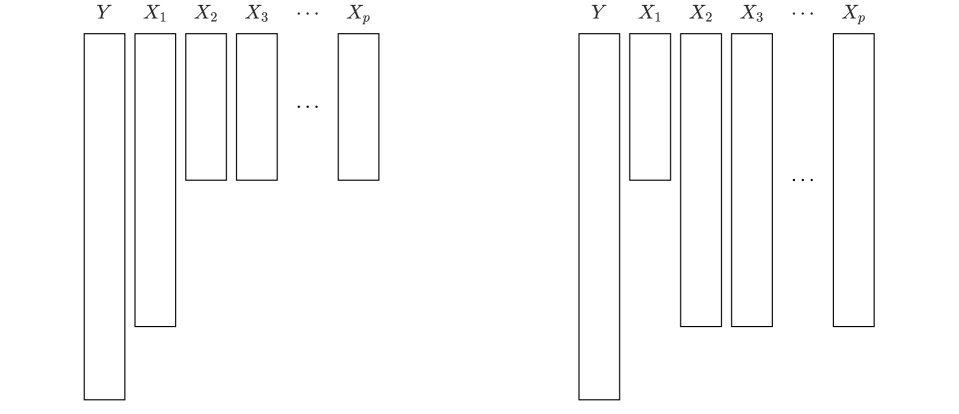
Figure 1: Illustration of two missing patterns.

3.2.1 Missing Pattern (a)

Consider the unit monotone missing pattern (a) shown in Figure 1(a). Let $q_{1}$ denote the observed proportion of $X_{1}$; $q_{-1}$ be the observed proportion of $X_{j}\,(j\geq 2)$. In addition, we assume available samples in $X_{2}$ to $X_{p}$ is a subset of $X_{1}\,(q_{1}>q_{-1})$ to have the monotone missing.

According to expressions (1) and (2), we obtain the asymptotic variance of $\hat{\beta}_{1}$ in both methods and calculate the difference $V_{D,\hat{\beta}_{1}}$. Let $f(\boldsymbol{\beta})\triangleq n\cdot V_{D,\hat{\beta}_{1}}$ denote the difference of asymptotic variance as a function of $\boldsymbol{\beta}$:

$$f(\boldsymbol{\beta})= -r_{11}^{2}\left(\frac{1}{q_{-1}}-\frac{1}{q_{1}}\right)\sum_{g=2}^{p}(\sigma_{1g}^{2}+2\kappa\sigma_{1g}^{2}+\sigma_{1}^{2}\sigma_{g}^{2}+\kappa\sigma_{1}^{2}\sigma_{g}^{2})\beta_{g}^{2}$$

$$\qquad-2r_{11}^{2}\left(\frac{1}{q_{-1}}-\frac{1}{q_{1}}\right)\sum_{g=2}^{p}\sum_{h=g+1}^{p}(\sigma_{1g}\sigma_{1h}+2\kappa\sigma_{1g}\sigma_{1h}+\sigma_{1}^{2}\sigma_{gh}+\kappa\sigma_{1}^{2}\sigma_{gh})\beta_{g}\beta_{h}$$

$$\qquad+(1+\kappa)\left(\frac{1}{q_{-1}}-\frac{1}{q_{1}}\right)\left(2r_{11}-r_{11}^{2}\sigma_{1}^{2}\right)\sigma^{2}.$$

The true coefficient $\beta_{1}$ is not involved in this expression. If $f(\boldsymbol{\beta})>0$, then the AC estimator is better.

We find that $\left(\frac{1}{q_{-1}}-\frac{1}{q_{1}}\right)$ is a key quantity in $f(\boldsymbol{\beta})$. NO matter which method is better, when we fix all other parameters, the larger the difference between $1/q_{-1}$ and $1/q_{1}$, the larger the difference of the two methods.

A special case is that all predictors are independent:

$$f(\boldsymbol{\beta})= \frac{1}{\sigma_{1}^{2}}(1+\kappa)\left(\frac{1}{q_{-1}}-\frac{1}{q_{1}}\right)\left(\sigma^{2}-\sum_{g=2}^{p}\sigma_{g}^{2}\beta_{g}^{2}\right).$$

The AC estimator is better when $f(\boldsymbol{\beta})>0$, so we have the following proposition:

Proposition 3.1:

In missing pattern (a), assuming all predictors are independent, the AC estimator is asymptotically better if and only if:

$$\sum_{g=2}^{p}\sigma_{g}^{2}\beta_{g}^{2}<\sigma^{2}.$$

We can rewrite the inequality as $\sum_{g=2}^{p}\left(\frac{\sigma_{g}\beta_{g}}{\sigma}\right)^{2}<1$, which means when the sum of squares of the standardized coefficients (except for $X_{1}$) are less than 1, the AC estimator of $\beta_{1}$ is better.

For the general case that predictors are not independent, we further discuss the behavior of $f(\boldsymbol{\beta})$ under two scenarios where $p=2$ or $p\geq 3$.

Scenario 1, $\bf p=2$:
In this scenario, we only have predictors $X_{1}$, $X_{2}$ in our model. Then $f(\boldsymbol{\beta})$ is simplified as:

$$f(\beta_{2})= -r_{11}^{2}(\sigma_{12}^{2}+2\kappa\sigma_{12}^{2}+\sigma_{1}^{2}\sigma_{2}^{2}+\kappa\sigma_{1}^{2}\sigma_{2}^{2})\left(\frac{1}{q_{-1}}-\frac{1}{q_{1}}\right)\beta_{2}^{2}$$

$$\qquad+(1+\kappa)\left(\frac{1}{q_{-1}}-\frac{1}{q_{1}}\right)\left(2r_{11}-r_{11}^{2}\sigma_{1}^{2}\right)\sigma^{2}.$$

It is obvious that when the constant term (that does not involve $\beta_{2}$) is negative, $f(\beta_{2})$ is always less than $0$ (i.e., CC is better). Therefore, we have the following proposition:

Proposition 3.2:

(See Appendix E (online supplemental material) for proof) In missing pattern (a) with two predictors, a sufficient condition that the CC estimator of $\beta_{1}$ is asymptotically better than the AC is:

$$\frac{\sigma_{1}^{2}\sigma_{2}^{2}}{\sigma_{12}^{2}}<2.$$

This proposition shows that if the correlation between two predictors is strong (i.e., $|\rho_{12}|>\frac{\sqrt{2}}{2}$), the AC estimator is always worse.

(a)                                                                        (b)

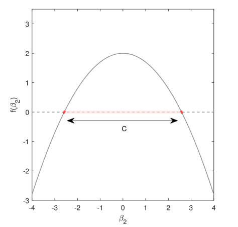
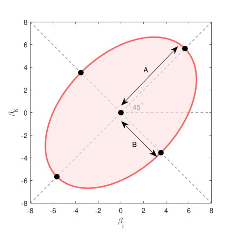
Figure 2: (a) $f(\beta_{2})$ in scenario 1 ($p=2$); (b) the projection of $f(\boldsymbol{\beta})=0$ in scenario 2 ($p\geq 3$).

When $\frac{\sigma_{1}^{2}\sigma_{2}^{2}}{\sigma_{12}^{2}}\geq 2$ (i.e., $|\rho_{12}|\leq\frac{\sqrt{2}}{2}$), the AC estimator has the possibility to be better than the CC as long as $\beta_{2}$ is not too far from $0$. In Figure 2(a), we plot function $f(\beta_{2})$ and find that $f>0$ iff $\beta_{2}$ lies in the interval between two intersections (the pink interval). This interval is symmetric around $0$ and we denote its length as $C$:

$$C =\sqrt{\frac{4\left(\sigma_{1}^{2}\sigma_{2}^{2}-2\sigma_{12}^{2}\right)\sigma^{2}}{\left(\frac{1+2\kappa}{1+\kappa}\sigma_{12}^{2}+\sigma_{1}^{2}\sigma_{2}^{2}\right)\sigma_{2}^{2}}}.$$

Table 1: How $C$ changes with parameters

Parameter	Segment 1	$C$	Segment 2	$C$
$\kappa$	$(-1/2,+\infty)$	$\searrow$
$\sigma_{12}$	$(-\sqrt{\sigma_{1}^{2}\sigma^{2}_{2}/2},0)$	$\nearrow$	$(0,\sqrt{\sigma_{1}^{2}\sigma^{2}_{2}/2})$	$\searrow$
$(\rho_{12})$	$(-\sqrt{2}/2,0)$	$\nearrow$	$(0,\sqrt{2}/2)$	$\searrow$
$\sigma_{2}^{2}$	$(2\sigma_{12}^{2}/\sigma_{1}^{2},M_{0}\ ^{a})$	$\nearrow$	$(M_{0},+\infty)$	$\searrow$
$\sigma_{1}^{2}$	$(2\sigma_{12}^{2}/\sigma_{2}^{2},+\infty)$	$\nearrow$
$\sigma^{2}$	$(0,+\infty)$	$\nearrow$

Note: ${}^{a}\ M_{0}=\left(2+\sqrt{8-2/(1+\kappa)}\right)\sigma_{12}^{2}/\sigma_{1}^{2}$

We list how $C$ changes with different parameters in Table 1. When the kurtosis parameter $\kappa$ increases, the interval length $C$ decreases, which means a heavy-tailed dataset favors the CC method. For the covariance structure, we find that a larger $\sigma_{1}^{2}$, $\sigma^{2}$ and a smaller $|\sigma_{12}|$ favors the AC estimator, but the effect of $\sigma_{2}^{2}$ is not monotone when fixing other parameters. In other words, increasing the variance of $X_{1}$ or the residual, and decreasing the correlation between $X_{1}$, $X_{2}$ make the AC estimator of $\beta_{1}$ has a smaller asymptotic variance.

Scenario 2, $\bf p\geq 3$:

In this scenario, we assume that $X_{j}\,(j\geq 2)$ are homoscedastic and has an exchangeable covariance structure. Their correlation with $X_{1}$ is exchangeable as well. Specifically, we assume that the variance of $X_{1}$ is $\sigma_{1}^{2}$; the variance of $X_{j}\,(j\geq 2)$ is $\sigma_{2^{\prime}}^{2}$; the covariance between $X_{1}$ and $X_{j}\,(j\geq 2)$ is $\sigma_{12^{\prime}}$; and the covariance between $X_{j}\,(j\geq 2)$ and $X_{k}\,(k\geq 2,k\neq j)$ is $\sigma_{2^{\prime}3^{\prime}}$. Then $f(\boldsymbol{\beta})$ is simplified as:

$$f(\boldsymbol{\beta})= -r_{11}^{2}(\sigma_{12^{\prime}}^{2}+2\kappa\sigma_{12^{\prime}}^{2}+\sigma_{1}^{2}\sigma_{2^{\prime}}^{2}+\kappa\sigma_{1}^{2}\sigma_{2^{\prime}}^{2})\left(\frac{1}{q_{-1}}-\frac{1}{q_{1}}\right)\sum_{g=2}^{p}\beta_{g}^{2}$$

$$\qquad-2r_{11}^{2}(\sigma^{2}_{12^{\prime}}+2\kappa\sigma_{12^{\prime}}^{2}+\sigma_{1}^{2}\sigma_{2^{\prime}3^{\prime}}+\kappa\sigma_{1}^{2}\sigma_{2^{\prime}3^{\prime}})\left(\frac{1}{q_{-1}}-\frac{1}{q_{1}}\right)\sum_{g=2}^{p}\sum_{h=g+1}^{p}\beta_{g}\beta_{h}$$

$$\qquad+(1+\kappa)\left(\frac{1}{q_{-1}}-\frac{1}{q_{1}}\right)\left(2r_{11}-r_{11}^{2}\sigma_{1}^{2}\right)\sigma^{2}.$$

We find that $f(\boldsymbol{\beta})$ is an elliptic paraboloid $\mathbb{R}^{p}$. When the constant term (that does not involve $\boldsymbol{\beta}$) in $f(\boldsymbol{\beta})$ is negative, $f(\boldsymbol{\beta})$ is always negative (See Appendix F (online supplemental material) for proof). So we have the following proposition:

Proposition 3.3:

(See Appendix E (online supplemental material) for proof) In missing pattern (a) with all assumptions above, a sufficient condition that the CC estimator of $\beta_{1}$ is asymptotically better than the AC is:

$$\{(p-2)\sigma_{2^{\prime}3^{\prime}}+\sigma_{2^{\prime}}^{2}\}\sigma_{1}^{2}<2(p-1)\sigma_{12^{\prime}}^{2}.$$

As $p\rightarrow\infty$, this condition becomes:

$$\frac{\sigma_{2^{\prime}3^{\prime}}\sigma_{1}^{2}}{\sigma_{12^{\prime}}^{2}}<2.$$

The condition $\sigma_{2^{\prime}3^{\prime}}\sigma_{1}^{2}<2\sigma_{12^{\prime}}^{2}$ is equivalent to $\rho_{2^{\prime}3^{\prime}}<2\rho_{12^{\prime}}^{2}$, where $\rho_{12^{\prime}}$, $\rho_{2^{\prime}3^{\prime}}$ is the correlation between $X_{1}$, $X_{j}\,(j\geq 2)$, and $X_{j}\,(j\geq 2)$, $X_{k}\,(k>1,k\neq j)$ respectively. This proposition shows that in a high dimensional dataset ($p$ is large) with missing pattern (a), if the correlation between $X_{1}$ and $X_{j}\,(j\geq 2)$ is too strong ($|\rho_{12^{\prime}}|>\sqrt{\frac{|\rho_{2^{\prime}3^{\prime}}|}{2}}$), the AC estimator is always worse.

Table 2: How $A$ changes with parameters

Parameter	Condition	Segment 1	$A$	Segment 2	$A$
$p$		$(I_{L},I_{R})\ ^{a}$	$\searrow$
$\kappa$		$(I_{L},+\infty)$	$\searrow$
$\sigma_{12^{\prime}}$		$(I_{L},0)$	$\nearrow$	$(0,I_{R})$	$\searrow$
$\sigma_{2^{\prime}3^{\prime}}$	$I_{L}<M_{1}\ ^{b}<I_{R}$	$(I_{L},0)$	$\nearrow$	$(0,I_{R})$	$\searrow$
	$I_{R}<M_{1}$	$(I_{L},I_{R})$	$\nearrow$
	$I_{L}>M_{1}$	$(I_{L},I_{R})$	$\searrow$
	$con\_1\ ^{c}>0\text{ and }I_{L}<M_{2}\ ^{b}$	$(I_{L},M_{2})$	$\nearrow$	$(M_{2},+\infty)$	$\searrow$
$\sigma_{2^{\prime}}^{2}$	$con\_1<0\text{ or }I_{L}>M_{2}$	$(I_{L},+\infty)$	$\searrow$
$\sigma_{1}^{2}$		$(I_{L},+\infty)$	$\nearrow$
$\sigma^{2}$		$(0,+\infty)$	$\nearrow$

Note: ${}^{a}\ I_{L},I_{R}$ are the minimum/maximum value for this parameter to take (See Appendix G (online supplemental material))
Note: ${}^{b}$ The expressions of $M_{1},M_{2}$ are in Appendix G (online supplemental material)
Note: ${}^{c}\ con\_1=(2+2p-2/(1+\kappa))\sigma_{12^{\prime}}^{2}+(3-p)\sigma_{1}^{2}\sigma_{2^{\prime}3^{\prime}}$

Table 3: How $B$ changes with parameters

Parameter	Condition	Segment 1	$B$	Segment 2	$B$
$p$		$(I_{L},I_{R})\ ^{a}$	$\searrow$
$\kappa$		$(I_{L},+\infty)$	$\rightarrow$
$\sigma_{12^{\prime}}$		$(I_{L},0)$	$\nearrow$	$(0,I_{R})$	$\searrow$
$\sigma_{2^{\prime}3^{\prime}}$	$2\sigma_{12^{\prime}}^{2}>\sigma_{1}^{2}\sigma_{2^{\prime}}^{2}\text{ and }I_{R}>M_{3}\ ^{b}$	$(I_{L},M_{3})$	$\nearrow$	$(M_{3},I_{R})$	$\searrow$
	$2\sigma_{12^{\prime}}^{2}<\sigma_{1}^{2}\sigma_{2^{\prime}}^{2}\text{ or }I_{R}<M_{3}$	$(I_{L},I_{R})$	$\nearrow$
	$2\sigma_{12^{\prime}}^{2}>\sigma_{1}^{2}\sigma_{2^{\prime}3^{\prime}}\text{ and }I_{L}<M_{4}\ ^{b}$	$(I_{L},M_{4})$	$\nearrow$	$(M_{4},+\infty)$	$\searrow$
$\sigma_{2^{\prime}}^{2}$	$2\sigma_{12^{\prime}}^{2}<\sigma_{1}^{2}\sigma_{2^{\prime}3^{\prime}}\text{ or }I_{L}>M_{4}$	$(I_{L},+\infty)$	$\searrow$
$\sigma_{1}^{2}$		$(I_{L},+\infty)$	$\nearrow$
$\sigma^{2}$		$(0,+\infty)$	$\nearrow$

Note: ${}^{a}\ I_{L},I_{R}$ are the minimum/maximum value for this parameter to take (See Appendix G (online supplemental material))
Note: ${}^{b}$ The expressions of $M_{3},M_{4}$ are in Appendix G (online supplemental material)

In Figure 2(b), we plot this ellipse whose center is at the origin and the major axis is rotated $45^{\circ}$ around the origin. When point $(\beta_{j},\beta_{k})$ lies in the ellipse (the pink region), then the AC estimator is better than the CC. Let $A$ and $B$ denote the length of the semi-major and semi-minor axes:

$$A =\sqrt{\frac{\left(-2(p-1)\sigma_{12^{\prime}}^{2}+(p-2)\sigma_{1}^{2}\sigma_{2^{\prime}3^{\prime}}+\sigma_{1}^{2}\sigma_{2^{\prime}}^{2}\right)\sigma^{2}}{\left((p-2)\sigma_{2^{\prime}3^{\prime}}+\sigma_{2^{\prime}}^{2}\right)\left(\frac{2+4\kappa}{1+\kappa}\sigma_{12^{\prime}}^{2}+\sigma_{1}^{2}\sigma_{2^{\prime}}^{2}+\sigma_{1}^{2}\sigma_{2^{\prime}3^{\prime}}\right)}},$$

$$B =\sqrt{\frac{\left(-2(p-1)\sigma_{12^{\prime}}^{2}+(p-2)\sigma_{1}^{2}\sigma_{2^{\prime}3^{\prime}}+\sigma_{1}^{2}\sigma_{2^{\prime}}^{2}\right)\sigma^{2}}{\left((p-2)\sigma_{2^{\prime}3^{\prime}}+\sigma_{2^{\prime}}^{2}\right)\left(\sigma_{1}^{2}\sigma_{2^{\prime}}^{2}-\sigma_{1}^{2}\sigma_{2^{\prime}3^{\prime}}\right)}}.$$

Similar to scenario 1, when $((p-2)\sigma_{2^{\prime}3^{\prime}}+\sigma_{2^{\prime}}^{2})\sigma_{1}^{2}\geq 2(p-1)\sigma_{12^{\prime}}^{2}$, the AC method has potential to be better than the CC. To be more specific, if setting $f(\boldsymbol{\beta})=0$, we get an ellipsoid in $\mathbb{R}^{p-1}$ space. This ellipsoid is symmetric around the origin and its projection onto any $(\beta_{j},\beta_{k})$-plane has the same shape and size. The projection curve on the $(\beta_{j},\beta_{k})$-plane is an ellipse and described by the following expression:

$$\left(\frac{1+2\kappa}{1+\kappa}\sigma_{12^{\prime}}^{2}+\sigma_{1}^{2}\sigma_{2^{\prime}}^{2}\right)(\beta_{j}^{2}+\beta_{k}^{2})+2\left(\frac{1+2\kappa}{1+\kappa}\sigma^{2}_{12^{\prime}}+\sigma_{1}^{2}\sigma_{2^{\prime}3^{\prime}}\right)\beta_{j}\beta_{k}=\left(\frac{2}{r_{11}}-\sigma_{1}^{2}\right)\sigma^{2}.$$

We list how $A$, $B$ change with different parameters in Table 3 and 3. In particular, when the number of predictors $p$ increases, both axes get shorter, resulting in a smaller ellipse that favors the CC method. Larger kurtosis parameter $\kappa$ also shrinks the ellipse, which means a heavy-tailed dataset impairs the performance of AC. In addition, we find that a larger $\sigma_{1}^{2}$, $\sigma^{2}$ and a smaller $|\sigma_{12^{\prime}}|$ favor AC estimator. The effect of $\sigma_{2^{\prime}}^{2}$, $\sigma_{2^{\prime}3^{\prime}}$ is not monotone. We conclude that a lower correlation between $X_{1}$ and other predictors, a larger variance of $X_{1}$ or the residual benefit the AC estimator.

3.2.2 Missing Pattern (b)

This missing pattern is shown in Figure 1(b). Let $q_{1}$ denote the observed proportion of $X_{1}$; $q_{-1}$ be the observed proportion of $X_{j}(j\geq 2)$. In addition, we assume available samples in $X_{1}$ is a subset of $X_{2}$ to $X_{p}$ ($q_{1}<q_{-1}$). A special case is that only variable $X_{1}$ has missing values ($q_{-1}=1$) which is called univariate missing. With expressions (1), (2), we obtain the asymptotic variance of $\hat{\beta}_{1}$ of two methods and the difference $V_{D,\hat{\beta}_{1}}$ is as follows:

$$n\cdot V_{D,\hat{\beta}_{1}} =\left(\frac{1}{q_{1}}-\frac{1}{q_{-1}}\right)\left\{n(r_{11}-r_{11}^{2}\sigma_{1}^{2})\sigma^{2}-c_{1}\beta_{1}^{2}\right\},$$

where

$$c_{1} =\sum_{\begin{subarray}{c}j=2\end{subarray}}^{p}r_{1j}^{2}\left(\sigma_{1j}^{2}+\sigma_{1}^{2}\sigma_{j}^{2}\right)+\kappa r_{1j}^{2}\sigma_{1}^{2}\sigma_{j}^{2}+2\kappa r_{1j}^{2}\sigma_{1j}^{2}$$

$$\qquad\quad+\sum_{\begin{subarray}{c}j=2\end{subarray}}^{p}\sum_{\begin{subarray}{c}k=j+1\end{subarray}}^{p}2r_{1j}r_{1k}\left(\sigma_{1j}\sigma_{1k}+\sigma^{2}_{1}\sigma_{jk}\right)+2\kappa r_{1j}r_{1k}\sigma^{2}_{1}\sigma_{jk}+4\kappa r_{1j}r_{1k}\sigma_{1j}\sigma_{1k}.$$

The asymptotic variance of $\hat{\beta}_{1}$ in the CC method is always equal or smaller than the AC method (See Appendix H (online supplemental material) for proof). The quantity $\left(\frac{1}{q_{1}}-\frac{1}{q_{-1}}\right)$ determines the difference of performance between two methods.

Proposition 3.4:

In missing pattern (b), the CC estimator of $\beta_{1}$ is asymptotically equal or better than the AC estimator.

This proposition implies that using extra data from $X_{2}$ to $X_{p}$ does not improve the estimation of $\beta_{1}$ asymptotically. The special case is that when $X_{1}$ is independent with other predictors, then both $(r_{11}-r_{11}^{2}\sigma_{1}^{2})=0$ and $c_{1}=0$ and thus we have the following proportion:

Proposition 3.5:

(See Appendix H (online supplemental material) for proof) In missing pattern (b), the AC and the CC have the same asymptotic performance if and only if $X_{1}$ is independent with other predictors.

3.3 Summary

Table 4: Summary table of the comparison in different scenarios.

Missing Pattern	$p$	Condition	AC	CC
pattern (a)		all predictors are independent, $\sum_{g=2}^{p}\sigma_{g}^{2}\beta_{g}^{2}<\sigma^{2}$	$\checkmark$
	$2$	$|\rho_{12}|>\sqrt{2}/2$		$\checkmark$
	$2$	large $\kappa$, $|\rho_{12}|$		$\bigstar$
	$2$	large $\sigma_{1}^{2}$, $\sigma^{2}$; small $|\beta_{2}|$	$\bigstar$
	$\geq 3$	special covariance ${}^{a}$; $\rho_{12^{\prime}}^{2}>\rho_{2^{\prime}3^{\prime}}/2$ ${}^{b}$ (large $p$)		$\checkmark$
	$\geq 3$	special covariance; large $p$, $\kappa$, $|\sigma_{12^{\prime}}|$		$\bigstar$
	$\geq 3$	special covariance; large $\sigma_{1}^{2}$, $\sigma^{2}$; small $|\beta_{g}|$ ($g\geq 2$)	$\bigstar$
pattern (b)		$X_{1}$ is independent with other predictors	same
		$X_{1}$ is not independent with other predictors		$\checkmark$

Note: ${}^{a}$ $X_{j}(j\geq 2)$ are homoscedastic and has an exchangeable covariance structure. Their correlation with $X_{1}$ is exchangeable as well.
Note: ${}^{b}$ This condition becomes $\{(p-2)\sigma_{2^{\prime}3^{\prime}}+\sigma_{2^{\prime}}^{2}\}\sigma_{1}^{2}<2(p-1)\sigma_{12^{\prime}}^{2}$ when $p$ is not large enough.
Note: $\checkmark$ represents the better estimator in this condition; $\bigstar$ represents this condition flavors the method, but it is not guaranteed to be better.