Measuring the Impact of Influence on Individuals: Roadmap to Quantifying Attitude

Abstract

Influence diffusion has been central to the study of the propagation of information in social networks, where influence is typically modeled as a binary property of entities: influenced or not influenced. We introduce the notion of attitude, which, as described in social psychology, is the degree by which an entity is influenced by the information. We present an information diffusion model that quantifies the degree of influence, i.e., attitude of individuals, in a social network. With this model, we formulate and study attitude maximization problem. We prove that the function for computing attitude is monotonic and sub-modular, and the attitude maximization problem is NP-Hard. We present a greedy algorithm for maximization with an approximation guarantee of $(1-1/e)$. Using the same model, we also introduce the notion of “actionable” attitude with the aim to study the scenarios where attaining individuals with high attitude is objectively more important than maximizing the attitude of the entire network. We show that the function for computing actionable attitude, unlike that for computing attitude, is non-submodular and however is approximately submodular. We present approximation algorithm for maximizing actionable attitude in a network. We experimentally evaluated our algorithms and study empirical properties of the attitude of nodes in network such as spatial and value distribution of high attitude nodes.

I Introduction

The proliferation of social networks and their influence in modern society led to a large body of research in several scientific domains that focus on utilizing and explaining the significance of the impact of social networks. One of the key problems investigated is to understand the diffusion of information/influence propagation in social networks. Diffusion refers to the (probabilistic) behavior of the interaction between the entities in the network describing when/how an entity is influenced by the actions of its neighbors.

Seminal works of Domingos and Richardson, and Kempe et al. proposed two popular models for information diffusion/influence propagation—Independent Cascade and Linear Threshold [11, 18]. In these models, a node of a network is said to be influenced if it receives the information originated at the seed set. This concept of influence is binary: an entity is either influenced or is not influenced. Real-world experience shows that not all influenced individuals are the same. I.e, some individuals are more strongly influenced by certain information compared to others. Thus, the strength of influence can vary from one individual to the other. This phenomenon has been pointed out in social sciences literature.

Within social psychology, two related concepts, attitudes and beliefs, are frequently studied to understand human behavior. Beliefs, which represent people’s ideas about the way the world is or should be, are commonly conceptualized as binary in nature, present or absent[13]. Throughout their lives, people acquire new beliefs, and sometimes, new beliefs replace old beliefs. In this way, people tend to acquire a very large number of beliefs over the life course. This notion of belief in social psychology, that is binary in nature, can be considered similar to the notion of “influence” in computational social network analysis which is also binary in nature.

Attitudes, on the other hand, are “latent predispositions to respond or behave in particular ways toward attitude objects” [12]. In contrast to beliefs, which are largely cognitive in nature, attitudes, have a cognitive, affective, and a behavioral component [30]. Being subjective in nature, attitudes can vary in strength such that a person can hold a very strong attitude or a weak attitude toward an object or concept, and thus attitude quantifies the strength of belief [2, 13]. Individuals acquire attitudes through experiences and exposure. In the case of exposure, a body of research shows that repeated exposure to an object/idea increases the likelihood that a person will adopt a more favorable attitude toward it [34]. Thus attitude being non-binary can be thought of strength of influence. Motivated by these studies, we study the problem of arriving at a mathematical model that captures the notion of attitude resulting from information propagation in social networks.

Our first contribution is to define a mathematical model for measuring attitude. Within social networks, people are often subjected to repeated exposures to information such as an anti-vaccine message, a pro-GMO message, or gun safety messaging. It has been observed that when an individual is exposed to a large number of, say, anti-vaccine messages, this increases the probability that that person will adopt a similar anti-vaccine attitude. Based on this, we postulate that the strength of influence or attitude of an individual, toward an object/concept, can be captured by the number of times the individual receives the information from its neighbors. In other words, if an already influenced individual is further provided with the same/similar influencing information, then the latter reinforces the learned belief of the individual, thus shaping and increasing his/her attitude. We use the number of reinforcements as a way to quantify the attitude.

Using this model, we define attitude of an individual and the total attitude of the network as functions from $2^{V}$ to reals ($2^{V}$ denotes the power set of nodes $V$ of the network). We denote the function that captures the total attitude of the network with $\sigma_{Att}(.)$ We study the computational complexity of the function $\sigma_{Att}$ and provide efficient algorithms to approximate it. We prove that this function is #P-hard and it is monotone and submodular. We provide an $(\epsilon,\delta)$-approximation algorithm for computing attitude with provable guarantees. We then formulate the attitude maximization problem–find a seed set $S$ of size $k$ that will result in maximum total attitude of the network. We first prove that the attitude maximization problem is NP-hard. Based on the monotonicity and submodularity of attitude, we propose a greedy algorithm that achieves a $(1-1/e)$ approximation guarantee.

We further introduce the concept of actionable attitude. The introduction of this concept is motivated by the fact that individuals with higher attitude (strongly influenced) are likely to act according to the attitude. This is particularly important in campaigns (such as political or gun-safety messaging), where motivated and dedicated volunteers are necessary to carry and spread the message (possibly beyond the social network); and such volunteers are the ones who are strongly influenced. Our second major contribution is the study of the underlying computational problem related to actionable attitude maximization. We prove that though the function for computing actionable attitude is not submodular, it is approximately submodular. Based on this we design efficient approximation algorithms to maximize the actionable attitude in a network.

II Related Work

Computational models of information diffusion in social networks is introduced and formalized in the seminal works of Domingos and Richardson [11] and Kempe, Kleinberg and Tardos [18]. There are two widely-studied probabilistic diffusion models: Independent Cascade (IC) model and Linear Threshold (LT) model. Kempe et al. [18] proved that the influence maximization problem is NP-hard, and also proved that a greedy algorithm achieves a $(1-1/e)$ approximation guarantee. The approximation guarantee of the greedy approach stems from the non-negativity, monotonicity and submodularity of the influence function. Since then several improvements have been proposed to make the greedy algorithm more practical and scalable  [20, 10, 17, 28, 33, 32, 7, 14]. Several variants of the influence maximization problem have been studied in the literature, since the work of Kempe et al. such as topic-aware influence maximization and targeted influence maximization [22, 8, 21, 4, 31, 15, 29, 25].

Enhancements to the basic influence propagation model have been proposed that take into account the opinions of users [35, 14, 9]. Liu et al. [23, 24] introduced PageRank based diffusion model, as a generalization of the basic IC model.

These models do not capture the notion of attitude/strength of influence that we seek to formalize. Aggarwal et al. [1] introduced a flow authority model to determine assimilation of information in a network. This model differs from the Independent Cascade and does not capture the notion of attitude due to repeated activations. Consider a network where node 1 has a directed edge to node 2 and 3, and node 2 has a directed edge to node 3, and edge probabilities are 1. Due to repeated activation, node 3 can receive information from nodes 1 and 2 and thus should have a higher attitude than nodes 1 and 2. However, in the flow-authority model all nodes will have equal probability of receiving ($p=1$) and does not distinguish node 3 from others whereas our proposed model will.

In [36], the authors discussed the problem of maximizing cumulative influence in a model where the same node can repeatedly activate his/her neighbor within a given time interval. This is realized by identifying a node to be newly activated in multiple iterations of the diffusion process (even if the node, under consideration may have been already activated). Such a model may lead to divergence in the computation of objective function, and hence, the computation is parameterized by a time interval. This distinguishes our model where only the newly activated nodes can alter the attitude of his/her neighbor; which ensures the convergence of computation of our objective function and allows the method to be step agnostic.

III Preliminaries

We describe the notation and definitions used frequently in this paper.

Definition 1 (Monotonicity & Submodularity).

Let $V$ be a ground set and $f:2^{V}\rightarrow\mathbb{R}$ be a set function, where $2^{V}$ denotes the power set of $V$. We say that $f$ is monotone if $f(S)\leq f(T)$ when $S\subseteq T$. We say that $f$ is submodular if for every pair of sets $S$ and $T$ with $S\subseteq T$ and every $x\notin T$, $f(S\cup\{x\})-f(S)\geq f(T\cup\{x\})-f(T)$.

We use $f(x|S)$ to denote the marginal gain of $x$ with respect to $S$, defined as $f(S\cup\{x\})-f(S)$.

Theorem 1 (Chernoff Bound).

Let $X_{1},X_{2}...X_{n}$ be independent identically distributed random variables taking value in the range $[0,1]$. $X=\sum_{i=1}^{n}X_{i}$. If $\mu=\mathbb{E}[X]$, then for $\lambda\in(0,1)$, $P[|X-\mu|\geq\mu\lambda]\leq 2exp(-\frac{\lambda^{2}}{2+\lambda}\cdot\mu)$

A social network is modeled as a weighted directed graph $G=(V,E)$ with parameters $p:e\in E\to[0,1]$, where V and E ($|V|=n$ and $|E|=m$) denote the set of nodes and edges, respectively. The function $p(e=(u,v))$ is the probability of node $u$ influencing/activating node $v$. This denotes probability that the information is successfully transferred from $u$ to $v$. We first recall the standard Independent Cascade model of information diffusion.

Definition 2.

[IC-Model] Information spreads via a random discrete process that begins at a set $S$ called seed set. Initially at step zero, all nodes in $S$ are activated/influenced. In each step, each newly activated node $u$ attempts to activate/influence its inactivated neighbor $v$ with probability $p(u,v)$. The diffusion process terminates when no new nodes are influenced in a step.

Given a set of nodes $S$, let $\sigma(S)$ be the expected number of nodes that are influenced at the end of the diffusion process when the seed set is $S$.

Influence Maximization Problem. Given a social network $G=(V,E)$, and an integer $k>0$, find a seed set $S\subseteq V$ of size $k$ such that $\sigma(S)$ is maximized.

Kempe et al. [18] proved that the influence maximization problem is NP-hard and showed that the function $\sigma(.)$ is monotone and submodular. Based on this, they designed a $(1-1/e)$-approximation algorithm for the influence maximization problem.

IV Modeling Attitude

In this section, we provide a mathematical model and definition to capture the notion of attitude.

Definition 3.

[Attitude-IC model (AIC)] The diffusion proceeds in discrete rounds starting from some set of seed-nodes $S$. Initially, all non-seed nodes have the attitude $0$ and every seed node starts with an attitude value of $1$. At each step, each newly influenced node $u$ tries to send information to each of its neighbor $v$ as per the edge probability $p(u,v)$. If $u$ succeeds, then $v$’s attitude is incremented by $1$; and its status is changed to influenced if it is not already influenced. When $u$ succeeds in sending information $v$, we say that the edge $\langle u,v\rangle$ is activated. The process terminates when no new nodes are influenced in a step.

Consider Figure 1 and let seed set is $S=\{a\}$. At step $t=0$, the attitude of $a$ is 1, $a$ tries to send information to $b,c$, succeeding with probability $1$. At $t=1$, the attitudes of $a,b,c$ are $1$. The newly activated nodes $b,c$ send information to their neighbors. Node $b$ succeeds and increments the attitude of nodes $a,c$. Simultaneously, $c$ succeeds and increments the attitude of nodes $a,b$. At $t=2$, the attitudes of $a,b,c$ are $3,2,2$ respectively. Since no new nodes are activated in this step, the diffusion ends.

Figure 1: An example showing inf-max problem $\neq$ attitude-max problem

Note that, unlike in the standard information diffusion model, where each activated node gets one chance to influence its un-influenced neighbors, in our model, each newly activated node tries to influence all its neighbors irrespective of whether they are already influenced or not. Thus an activated node can receive information from a newly activated node and this captures the notion of repeated exposure or reinforcement, which, in turn, results in an increase of the recipient’s attitude.

For any set $S\subseteq V$ of nodes, we use $\mathtt{Att}_{v}(S)$ to denote the final attitude of node $v$ when the seed set is $S$. Note that this is a random variable and let $\mathbb{E}[\mathtt{Att}_{v}(S)],$ denote the expectation of $\mathtt{Att}_{v}(S)$. We define $\mathtt{AttIn}(S)$ as $\sum_{v\in V}\mathtt{Att}_{v}(S)$. The total expected attitude of the network resulting from diffusion starting at seed $S$ is $\sigma_{\mathtt{Att}}(S)=\mathbb{E}[\mathtt{AttIn}(S)]$. Observe that by l linearity of expectation, $\sigma_{\mathtt{Att}}(S)=\sum_{v\in V}\mathbb{E}[\mathtt{Att}_{v}(S)].$

By overloading notation, we often interpret $G$ as a distribution over unweighted directed graphs, each edge $e=(u,v)$ is realized independently with probability $p(u,v)$. We write $g\sim G$ to denote that an unweighted graph $g$ is drawn from this graph distribution $G$. Given a set of nodes $S\subseteq V$ and a graph $g$, we use

1. $R^{S}_{g}$ to denote the set of nodes reachable from $S$ in $g$.

2. $E^{S}_{g}=\{e=(u,v)|u,v\in R^{S}_{g}$ and $e\in g\}$ is the set of activated edges in $g$ due to diffusion from $S$. Let $E^{S}_{g,v}$ be the set of activated edges of the form $\langle.,v\rangle$.

3. $\mathtt{AttIn}_{g}(S)$ to denote the attitude induced by $S$ in graph $g$ and is equal to $\sum_{v\in V}\mathtt{Att}_{g,v}(S)$, where $\mathtt{Att}_{g,v}(S)$ is the attitude of $v$ in the graph $g$ computed as the number of activated incoming edges to $v$.

We next prove a critical theorem that will be used in our subsequent proofs. Informally, this theorem states that the $\sigma_{\mathtt{Att}}(S)$ is the expected number of activated edges.

Theorem 2.

If $g\sim G$ then for any $S\subseteq V$, $\sigma_{\mathtt{Att}}(S)=|S|+\sum_{g\sim G}|E^{S}_{g}|\times Pr(g\sim G),$ and $\mathbb{E}[\mathtt{Att}_{v}(S)]=\sum_{g\sim G}|E^{S}_{g,v}|\times Pr(g\sim G)$.

Proof.

Recall that, a node $u$ contributes to the attitude of its neighbor $v$, if $u$ is influenced and it is successful in “passing” on the influence to $v$ (irrespective of whether $v$ is already influenced or not) via the directed edge $\langle u,v\rangle$. We refer to such an edge as an activated edge.

Let $g$ be a graph drawn as per the distribution. Note that $g$ corresponds to a particular diffusion process. In $g$, if a node $v$ is not reachable from $S$, it means $v$ is not activated in that diffusion process, and its incoming edges, if any, are not activated. Thus the attitude of such a node is $0$. On the other hand, if a node $v$ is reachable from $S$ in $g$, it means $v$ is activated in the diffusion process. If $x$ is the number of incoming edges to $v$ in $G$, this means that $v$ received information through its neighbors $x$ times. Thus the attitude of $v$ is $x$ in this diffusion process. Thus node $v$’s attitude is the number of activated incoming edges of $v$. Let $N(v)$ denote the number of activated incoming edges of $v$. Then $\mathtt{AttIn}_{g}(S)$ is equal to

$$\begin{array}[]{r@{\ =\ }l}\displaystyle\sum_{v\in V}\mathtt{Att}_{g,v}(S)&\displaystyle\sum_{v\in R^{S}_{g}}\mathtt{Att}_{g,v}(S)+\sum_{v\notin R^{S}_{g}}\mathtt{Att}_{g,v}(S)\\[5.0pt] &\displaystyle|S|+\sum_{v\in R_{g}^{S}}N(v)+0=|S|+|E^{S}_{g}|\end{array}$$

The term $|S|$ is due to the fact that every seed node starts with an attitude value of $1$. This leads to

$$\begin{array}[]{r@{\ = \ } l}\sigma_{\mathtt{Att}}(S)&\mathbb{E}[\mathtt{AttIn}(S)]\\ &\mathbb{E}_{g\sim G}[\mathtt{AttIn}_{g}(S)]=|S|+\displaystyle\sum_{g\sim G}|E^{S}_{g}|\times Pr(g\sim G)\end{array}$$

The second equality stated in the theorem follows from similar arguments. Let $g$ be a graph drawn as per the distribution. Observe that $\mathtt{Att}_{g,v}(S)=|E^{S}_{g,v}|$. This leads to:

$$\begin{array}[]{r@{\ = \ } l}\mathbb{E}[\mathtt{Att}_{v}(S)]&\sum_{g\sim G}\mathtt{Att}_{g,v}(S)\times Pr(g\sim G)\\ &\sum_{g\sim G}|E^{S}_{g,v}|\times Pr(g\sim G)\end{array}$$

∎

IV-A Properties of Attitude

In this section, we investigate several properties of the function $\sigma_{\mathtt{Att}}(.)$. We first show that the $\sigma_{\mathtt{Att}}$ is monotone and submodular

Theorem 3.

Under the AIC model, $\sigma_{\mathtt{Att}}(.)$ is a monotone, non-decreasing function function.

Proof.

Let $g\sim G$ and $S\subseteq T\subseteq V$. We observe $R^{S}_{g}\subseteq R^{T}_{g}$ since $S\subseteq T$. Thus, $E^{S}_{g}\subseteq E^{T}_{g}$ and $|E^{S}_{g}|\leq|E^{T}_{g}|$. Therefore, $\sigma_{\mathtt{Att}}(S)\leq\sigma_{\mathtt{Att}}(T)$. ∎

Theorem 4.

Under the AIC model, $\sigma_{\mathtt{Att}}(.)$ is a submodular function.

Proof.

Let $g\sim G$, $S\subseteq T\subseteq V$ and $u\notin T$. Our objective is to prove that

$$\begin{array}[]{l}\sigma_{\mathtt{Att}}(S\cup\{u\})-\sigma_{\mathtt{Att}}(S)\\ =\displaystyle\sum_{g\sim G}(|E^{S\cup\{u\}}_{g}|-|E^{S}_{g}|)\times Pr(g\sim G)\\[5.0pt] \geq\sigma_{\mathtt{Att}}(T\cup\{u\})-\sigma_{\mathtt{Att}}(T)\\[5.0pt] =\displaystyle\sum_{g\sim G}(|E^{T\cup\{u\}}_{g}|-|E^{T}_{g}|)\times Pr(g\sim G)\end{array}$$

Since $Pr(g\sim G)\geq 0$, the proof obligation is

$$\forall g\sim G\ \ |E^{S\cup\{u\}}_{g}|-|E^{S}_{g}|\geq|E^{T\cup\{u\}}_{g}|-|E^{T}_{g}|$$

Observe that,

$$\begin{array}[]{l}|E^{S\cup\{u\}}_{g}|-|E^{S}_{g}|=|E^{S\cup\{u\}}_{g}\setminus E^{S}_{g}|\mbox{ and }\\ |E^{T\cup\{u\}}_{g}|-|E^{T}_{g}|=|E^{T\cup\{u\}}_{g}\setminus E^{T}_{g}|\end{array}$$

$R_{g}^{S}\subseteq R_{g}^{T}$ and $E^{S}_{g}\subseteq E^{T}_{g}$.

For any $g\sim G$, if $e\in E^{T\cup\{u\}}_{g}\setminus E^{T}_{g}$ then $e\notin E^{T}_{g}$ and $e\in E^{\{u\}}_{g}$. Since $E^{S}_{g}\subseteq E^{T}_{g},e\notin E^{S}_{g}$. We know that $e\in E^{\{u\}}_{g}$ and thus $e\in E^{S\cup\{u\}}_{g}$. Therefore, $e\in E^{S\cup\{u\}}_{g}\setminus E^{S}_{g}$ and thus $E^{T\cup\{u\}}_{g}\setminus E^{T}_{g}\subseteq E^{S\cup\{u\}}_{g}\setminus E^{S}_{g}$. This leads to $|E^{S\cup\{u\}}_{g}\setminus E^{S}_{g}|\geq|E^{T\cup\{u\}}_{g}\setminus E^{T}_{g}|$. ∎

The following result establishes the hardness of computing $\sigma_{\mathtt{Att}}$.

Theorem 5.

Under the AIC model, given $G=(V,E)$ and a seed $S\subseteq V$, computing the values of the following is #P-Hard: 1) $\sigma_{\mathtt{Att}}(S)$, 2) $\mathbb{E}[\mathtt{Att}_{v}(\cdot)],\forall v\in V$.

Proof.

Let $\sigma(S)$ be the influence of $S$ under the IC model. Computation of $\sigma(S)$ is known to be a #P-Hard problem  [10]. Assume that there exists a function $A(G,S)$ that computes $\sigma_{\mathtt{Att}}(S)$. Let $a_{1}=A(G,S)$. Add a new vertex $v_{new}$ to $G$. $\forall v\in V$, add an edge $(v,v_{new})$ and set $p(v,v_{new})=1$. This results in graph $G^{\prime}$. Let $a_{2}=A(G^{\prime},S)$. $a_{2}-a_{1}=\sum_{v\in V}P(S\texttt{ activates v})=\sigma(S)$. Therefore, $A$ can be used to compute $\sigma(S)$. Similarly, let $A^{\prime}(G,v)$ be a function that computes $\mathbb{E}[\mathtt{Att}_{v}(S)]$. $A^{\prime}(G^{\prime},v_{new})$ will be able to compute $\sigma(S)$ as $\mathbb{E}[\mathtt{Att}_{v_{new}}(S)]=\sigma(S)$. Similar arguments prove that computing $\mathbb{E}[\mathtt{Att}_{v}(\cdot)]$ is also #P-hard. ∎

IV-B Attitude Computation

From Theorem 5, it follows that computing $\sigma_{\mathtt{Att}}(S)$ exactly is computationally infeasible. In this section, we provide efficient approximation algorithms to estimate $\sigma_{\mathtt{Att}}(S)$. Borgs et. al. [7] introduced Reverse Influence Sampling (RIS), which has been used to develop efficient Influence Maximization algorithms [33, 32, 28, 16]. Using ideas from these works, combining with Theorem 2, we introduce a Reverse Attitude Sampling (RAS) technique.

Recall that $g$ denotes the un-weighted graph drawn from the random graph distribution $G$. We write $g^{T}$ to denote the transpose of $g$. The following lemma and theorem establish the relationship between an edge being activated by some nodes in any set $S\subseteq V$ and the reachability of some node in $S$ from reverse of the same edges in $g^{T}$; this relationship is key to the correctness of RAS technique.

Lemma 1.

Let $e=(x,y)$ be an arbitrary edge in $G$, $R^{\{x\}}_{g^{T}}$ be the set of nodes reachable from $x$ in $g^{T}$, where $g^{T}$ is the transpose of un-weighted graph $g$ drawn from random distribution $G$. Then for any $S\subseteq V$, $P[S\text{ activates }e\mbox{ in }g]=P[S\cap R^{\{x\}}_{g^{T}}\neq\emptyset]$

Both events, $S\text{ activates }e\mbox{ in }g$ and $S\cap R^{\{x\}}_{g^{T}}\neq\emptyset$ requires drawing $g$ from $G$ such that there exists a path between some node in $S$ and node $x$ (from $S$ to $x$ in $g$ and $x$ to $S$ in $g^{T}$). The probability of occurrence of such events are identical, as the probabilities of edges in $g$ and their reverse in $g^{T}$ are equal.

The following theorem relates the $\sigma_{\mathtt{Att}}(S)$ to reverse attitude sampling.

Theorem 6.

Given a graph $G=(V,E)$, for any $S\subseteq V$, and for any $v\in V$, let $\mathbb{E}(\mathtt{Att}_{v}(S))$ denotes the expected attitude of v induced by $S$. Then, $\mathbb{E}(\mathtt{Att}_{v}(S))=|InDegree(v)|\times P_{g\sim G,e=(u,v)\sim E}[S\cap R^{\{u\}}_{g^{T}}~{}|~{}e\in g]$ and $\sigma_{\mathtt{Att}}(S)=|S|+|E|\times P_{g\sim G,e=(x,y)\sim E}[S\cap R^{\{x\}}_{g^{T}}~{}|~{}e\in g]$

Proof.

With respect to a set $S$ and a node $v$, we will define the random variable

$$X^{(u,v)}_{g}=\left\{\begin{array}[]{ll}1&\mbox{if }(u,v)\in E^{S}_{g}\\ 0&\mbox{otherwise}\end{array}\right.$$

Therefore, by Theorem 2, it follows that

$$\mathbb{E}(\mathtt{Att}_{v}(S))=\displaystyle\sum_{(u,v)\in E}\mathbb{E}_{g\sim G}[X^{(u,v)}_{g}].$$

Note that,

$$\begin{split}\mathbb{E}_{g\sim G}[X^{(u,v)}_{g}]&=P_{g\sim G}[\exists w\in S.\ u\in R^{\{w\}}_{g}\land(u,v)\in g]\\ &=P_{g\sim G}[\exists w\in S.\ w\in R^{\{u\}}_{g^{T}}\land(u,v)\in g]\end{split}$$

By linearity of expectation, we have:

$$\begin{split}\mathbb{E}(\mathtt{Att}_{v}(S))&=\sum_{(u,v)\in E}\mathbb{E}_{g\sim G}[X^{(u,v)}_{g}]\\ &=\sum_{(u,v)\in E}P_{g\sim G}[\exists w\in S.\ w\in R^{\{u\}}_{g^{T}}\land(u,v)\in g]\\ &=|\mbox{InDegree}(v)|\!\times\!P_{g\sim G,e=(u,v)\sim E}[S\cap R^{\{u\}}_{g^{T}}|e\in g]\end{split}$$

We present the proof of the second equality. With respect to a set $S$, we will define the random variable $X^{e}_{g}=1$ if $e\in E^{S}_{g}$, otherwise it is zero. Therefore, by Theorem 2, we have $\sigma_{\mathtt{Att}}(S)=\mathbb{E}_{g\sim G}[\mathtt{AttIn}_{g}(S)]=|S|+\displaystyle\sum_{e\in E}\mathbb{E}_{g\sim G}[X^{e}_{g}]$. Note that,

$$\begin{split}\mathbb{E}_{g\sim G}[X^{e}_{g}]&=P_{g\sim G}[\exists u\in S.\ x\in R^{\{u\}}_{g}\land e=(x,y)\in g]\\ &=P_{g\sim G}[\exists u\in S.\ u\in R^{\{x\}}_{g^{T}}\land e=(x,y)\in g]\end{split}$$

By linearity of expectation, we have:

$$\begin{split}\sigma_{\mathtt{Att}}(S)&=|S|+\sum_{e\in E}\mathbb{E}_{g\sim G}[X^{e}_{g}]\\ &=|S|+\sum_{e\in E}P_{g\sim G}[\exists u\in S.\ u\in R^{\{x\}}_{g^{T}}\land e=(x,y)\in g]\\ &=|S|+|E|\!\times\!P_{g\sim G,e\in E}[\exists u\in S.\ u\in R^{\{x\}}_{g^{T}}\land e=(x,y)\in g]\end{split}$$

∎

The above properties pave way for the RAS technique. We proceed by introducing Random Reverse Reachable Set in the context of the AIC model. Given a graph $G=(V,E)$, we construct Random Reverse Reachable Set ($RR$) of nodes in $V$ as follows. Consider the transpose of $G$, $G^{T}=(V,E^{T})$, where the probability annotation for any edge in $E$ remains unchanged in the reverse of that edge in $E^{T}$.

We now describe a procedure to generate Random Reverse Reachable Sets (RR Sets):
Generate RR Set. Randomly pick an edge $e=(v,u)\in E^{T}$. Then with probability $p(e)$, add the node $u$ to $RR$. For any $u$ is added to $RR$, for each outgoing edge from $u$ in $G^{T}$, add the destination with corresponding edge probability. The process continues till no node is added to $RR$.

From Theorem 6, we obtain the following lemma.

Lemma 2.

$\sigma_{\mathtt{Att}}(S)=|S|+|E|\times P_{RR\sim\mathcal{R}}[S\cap RR\neq\emptyset]$

Data: Graph $G=(V,E)$, $S\subseteq V$

begin

       $\mathcal{R}=\mbox{Generate $\beta$ RR Sets using {\bf Generate RR Set}}$

       $X=|\{RR\in\mathcal{R}~{}|~{}S\cap RR\neq\emptyset\}|$

      

      return $\displaystyle\frac{|E|\cdot X}{\beta}$

      

Algorithm 1 Estimate $\sigma_{\mathtt{Att}}(S)$

Lemma  2 allows us to design Algorithm  1 to estimate $\sigma_{\mathtt{Att}}(S)$. In order to get a good estimate, we will obtain a lower bound for $\beta$ in Algorithm  1. Let $m=|E|$. Let $X_{i}$ be a random variable that takes value $1$ if the $i$-th $RR$ Set contains an element of $S$. Otherwise, $X_{i}=0$. Clearly each $X_{i}$ is independent and $X=\sum_{i=1}^{\beta}X_{i}$. Note, $\mathbb{E}[X]=\displaystyle\frac{\beta\sigma_{\mathtt{Att}}(S)}{m}$

$$\begin{array}[]{cl}&P[|\widehat{\sigma_{\mathtt{Att}}}(S)-\sigma_{\mathtt{Att}}(S)|\geq\epsilon\sigma_{\mathtt{Att}}(S)]\\ =&P[|m\displaystyle\frac{X}{\beta}-\sigma_{\mathtt{Att}}(S)|\geq\epsilon\sigma_{\mathtt{Att}}(S)]\\ =&P[|X-\displaystyle\frac{\beta\sigma_{\mathtt{Att}}(S)}{m}|\geq\epsilon\cdot\displaystyle\frac{\beta}{m}\sigma_{\mathtt{Att}}(S)]\\ \leq&2exp(-\displaystyle\frac{\epsilon^{2}\beta\sigma_{\mathtt{Att}}(S)}{(2+\epsilon)m})\end{array}$$

The last inequality follows by applying Chernoff Bounds with $\lambda=\epsilon$. Let $\delta=2exp(-\displaystyle\frac{\epsilon^{2}\beta\sigma_{\mathtt{Att}}(S)}{(2+\epsilon)m})$. When $\beta\in\theta(\frac{m}{\epsilon^{2}\sigma_{\mathtt{Att}}(S)}\cdot log(\frac{1}{\delta})$, Algorithm  1 estimates $\sigma_{\mathtt{Att}}(S)$ within a relative error of $\epsilon$ with probability $1-\delta$.

V Attitude Maximization Problem

Having defined Attitude under the AIC-model, a natural problem arises: How do we find a set of users, who can influence the network in a way that maximizes the attitude of the network? We model this as the Attitude Maximization Problem:

Problem 1.

Attitude Maximization Problem: Given a graph $G=(V,E)$, a number $k$, find $S\subseteq V$ of size at most $k$ such that $\sigma_{\mathtt{Att}}(S)$ is maximized.

Theorem 7.

Under the AIC model, the attitude maximization problem, i.e., computing $\mathtt{argmax_{S\subseteq V,|S|\leq k}}\ \sigma_{\mathtt{Att}}(S)$, is NP-hard.

Proof.

Our proof relies on reduction of influence maximization problem (a known NP-Hard problem) to attitude maximization problem.

We consider the influence maximization problem on directed Bi-partite graphs (edges from left nodes to right nodes) with edge probabilities 1. That is, $G=(V,E)$, where $V=X\cup Y$, $X\cap Y=\emptyset,E=\{(u,v)|u\in X,v\in Y\},$ and $\forall e\in E$ $p(e)=1$. Kempe et al. [18] proved that influence maximization problem on such restricted class of graphs is also NP-hard.

We extend the bipartite graph $G$ to construct an instance $G^{\prime}=(V^{\prime},E^{\prime})$ for the attitude maximization problem, where $V^{\prime}=V\cup Z,Z=\{z_{1},z_{2},\ldots,z_{2|E|}\}$ and for each $y\in Y$, there exists an edge to each $z\in Z$ with the edge probability $1$.

Suppose that there is an algorithm for computing a set $S\subseteq X$ of size $k$ that maximizes $\sigma_{\mathtt{Att}}(S)$. If $L$ nodes in the set $Y$ are influenced by $S$, then $\sigma_{\mathtt{Att}}(S)\leq L\times 2|E|+|E|$. (Each edge from an influenced node in $Y$ contributes to the attitude of each nodes in $Z$, and the overall attitude of nodes in $Y$ can be at most $|E|$, the number of edges between $X$ and $Y$.)

Assume that $S$ does not induce maximum influence in $G$, i.e., there exists some $S^{\prime}\neq S$ for which $G$ is maximally influenced. In other words, $S^{\prime}$ influences at least $L+1$ nodes in $Y$. Therefore, if $S^{\prime}$ is used as seed in $G^{\prime}$, then it would have induced the overall attitude of nodes in $Z$ to be $(L+1)\times 2|E|$. This implies, $S^{\prime}\neq S$ is a set of size $|k|$ that maximizes $\sigma_{\mathtt{Att}}(S^{\prime})$ in $G^{\prime}$, leading to a contradiction.

Therefore, if any algorithm that computes a set $S$ that maximizes attitude in $G^{\prime}$, then $S$ must also maximize influence in $G$. ∎

Before we proceed to present an approximation algorithm for the attitude maximization problem, we first prove that influence maximization problem is different from the attitude maximization problem. In particular, we prove that the optimal solution for the influence maximization problem is not an optimal solution for the attitude maximization problem. Consider the from Figure 1. When $k=1$, the best seed set for the influence maximization is $\{d\}$ whereas the best seed set for the attitude maximization is any of $\{a\},\{b\}$ or $\{c\}$. Thus,

Theorem 8.

An optimal solution to the influence maximization problem is not an optimal solution to the attitude maximization problem.

Nemhauser et. al.  [27] proved the greedy strategy to maximize a non-decreasing, monotone, and submodular function outputs a $(1-1/e)$-approximate solution. Recall that $\sigma_{\mathtt{Att}}(\cdot)$ is in fact a non-decreasing, monotone and submodular function. However, the challenge lies in efficiently estimating $\sigma_{\mathtt{Att}}(\cdot)$. Motivated by this, we design a RAS-based approximation algorithm.

Data: Graph $G=(V,E)$, $k$

Result: Seed Set $S$

begin

       $\mathcal{R}=\mbox{Generate $\beta$ RR Sets using {\bf Generate RR Set}}$

       Mark all the sets in $\mathcal{R}$ as uncovered

       while $|S|\leq k$ do

             Find $v$ that covers maximum uncovered sets in $\mathcal{R}$

             Mark sets covered by $v$ as covered

             Add $v$ to $S$

            

      return $S$

      

Algorithm 2 $(1-1/e-\epsilon)$-approximate algorithm

Algorithm 2 is our greedy algorithm for the attitude maximization problem. The algorithm works by generating $\beta$ random RR Sets. With the goal now to find $S$ that covers the maximum RR Sets, the problem is transformed to the Maximum Coverage problem. The greedy algorithm, when applied to the Maximum Coverage problem, provides a $(1-1/e)$-approximate solution. We have the following result on the approximation guarantee Algorithm 2.

Theorem 9.

When $\beta\in\theta(\frac{|E|(1+1\epsilon)}{\epsilon^{2}\sigma_{\mathtt{Att}}(S^{*})}(log{n\choose k}-log(\delta)))$, Algorithm 2 outputs a seed set $S_{k}$ such that

$$\sigma_{\mathtt{Att}}(S_{k})\geq\left(1-\displaystyle\frac{1}{e}-\epsilon\right)\sigma_{\mathtt{Att}}(S^{*})$$

with probability at least $1-\delta$.

Proof.

We will prove that the algorithm produces a $(1-1/e-\epsilon)$-approximate solution with high probability.

First, we derive the bound for $\beta$ that is sufficient for estimating $\sigma_{\mathtt{Att}}(S)$ within a pre-specified error margin $\epsilon$, in the context of computing the maximal overall attitude.

Consider any $S\subseteq V$ of size $k$. Let $X$ be the cardinality of $\{RR\in\mathcal{R}|RR\cap S\neq\phi\}$. $\widehat{\sigma_{\mathtt{Att}}}(S)=|E|\times\displaystyle\frac{X}{\beta}$ is a an estimate for $\sigma_{\mathtt{Att}}(S)$. Let $\mu=\displaystyle\frac{\beta\cdot\sigma_{\mathtt{Att}}(S)}{|E|}$ and $\sigma_{\mathtt{Att}}(S^{*})$ be the maximum expected attitude induced by any set of size $k$.

$$\begin{array}[]{cl}&P\left[|\widehat{\sigma_{\mathtt{Att}}}(S)-\sigma_{\mathtt{Att}}(S)|\geq\displaystyle\frac{\epsilon\sigma_{\mathtt{Att}}(S^{*})}{2}\right]\\ =&P\left[|E|\cdot\displaystyle\frac{X}{\beta}-\sigma_{\mathtt{Att}}(S)|\geq\displaystyle\frac{\epsilon\sigma_{\mathtt{Att}}(S^{*})}{2}\right]\\ =&P\left[|\displaystyle\frac{X}{\beta}-\displaystyle\frac{\sigma_{\mathtt{Att}}(S)}{|E|}|\geq\displaystyle\frac{\epsilon\sigma_{\mathtt{Att}}(S^{*})}{2|E|}\right]\\ =&P\left[|X-\mu|\geq\displaystyle\frac{\epsilon\sigma_{\mathtt{Att}}(S^{*})\cdot\beta}{2|E|}\right]\\ =&P\left[|X-\mu|\geq\displaystyle\frac{\epsilon\sigma_{\mathtt{Att}}(S^{*})\cdot\beta\sigma_{\mathtt{Att}}(S)}{2\sigma_{\mathtt{Att}}(S)|E|}\right]\\ \end{array}$$

We apply Chernoff Bounds with $\lambda=\displaystyle\frac{\epsilon\sigma_{\mathtt{Att}}(S^{*})}{2\sigma_{\mathtt{Att}}(S)}$,

$$\begin{array}[]{cl}&P\left[|X-\mu|\geq\lambda\mu\right]<2exp\left(-\displaystyle\frac{\lambda^{2}}{2+\lambda}\mu\right)\\ =&2exp\left(-\displaystyle\frac{\epsilon^{2}(\sigma_{\mathtt{Att}}(S^{*}))^{2}}{(2+\lambda)\times 4(\sigma_{\mathtt{Att}}(S))^{2}}\mu\right)\\ =&2exp\left(-\displaystyle\frac{\epsilon^{2}(\sigma_{\mathtt{Att}}(S^{*}))^{2}}{(2+\lambda)\times 4(\sigma_{\mathtt{Att}}(S))^{2}}\displaystyle\frac{\beta\cdot\sigma_{\mathtt{Att}}(S)}{|E|}\right)\\ =&2exp\left(-\displaystyle\frac{\epsilon^{2}(\sigma_{\mathtt{Att}}(S^{*}))^{2}}{(2+\lambda)\times 4\sigma_{\mathtt{Att}}(S)}\displaystyle\frac{\beta}{|E|}\right)\\ =&2exp\left(-\displaystyle\frac{\epsilon^{2}(\sigma_{\mathtt{Att}}(S^{*}))^{2}}{|E|(8\sigma_{\mathtt{Att}}(S)+2\epsilon\sigma_{\mathtt{Att}}(S^{*}))}\beta\right)\\ \leq&2exp\left(-\displaystyle\frac{\epsilon^{2}(\sigma_{\mathtt{Att}}(S^{*}))^{2}}{|E|(8\sigma_{\mathtt{Att}}(S^{*})+2\epsilon\sigma_{\mathtt{Att}}(S^{*}))}\beta\right)\\ =&2exp\left(-\displaystyle\frac{\epsilon^{2}\sigma_{\mathtt{Att}}(S^{*})}{|E|(8+2\epsilon)}\beta\right)\end{array}$$

The inequality follows from $\sigma_{\mathtt{Att}}(S^{*})\geq\sigma_{\mathtt{Att}}(S)$. We would like the probability of this event to be at most $\displaystyle\frac{\delta}{{n\choose k}}$. Proceeding further,

$$\begin{array}[]{rcl}2exp\left(-\displaystyle\frac{\epsilon^{2}\sigma_{\mathtt{Att}}(S^{*})}{|E|(8+2\epsilon)}\beta\right)&\leq&\displaystyle\frac{\delta}{{n\choose k}}\\ -\displaystyle\frac{\epsilon^{2}\sigma_{\mathtt{Att}}(S^{*})}{|E|(8+2\epsilon)}\beta&\leq&log\left(\displaystyle\frac{\delta}{2{n\choose k}}\right)\\ \end{array}$$

This implies that

$$\beta\geq\frac{|E|(8+2\epsilon)}{\epsilon^{2}\sigma_{\mathtt{Att}}(S^{*})}\left[log(2)+log{n\choose k}-log(\delta)\right]$$

$$\begin{array}[]{rcl}\beta&\geq&-\displaystyle\frac{|E|(8+2\epsilon)}{\epsilon^{2}\sigma_{\mathtt{Att}}(S^{*})}log\left(\displaystyle\frac{\delta}{2{n\choose k}}\right)\\[10.00002pt] &=&-\displaystyle\frac{|E|(8+2\epsilon)}{\epsilon^{2}\sigma_{\mathtt{Att}}(S^{*})}\left[log(\delta)-log(2)-log{n\choose k}\right]\\[10.00002pt] &=&\displaystyle\frac{|E|(8+2\epsilon)}{\epsilon^{2}\sigma_{\mathtt{Att}}(S^{*})}\left[log(2)+log{n\choose k}-log(\delta)\right]\end{array}$$

Now that we have a lower bound for $\beta$, we can use the union bound to show that this number of $RR$ sets is sufficient to ensure that all sets of size $k$ is within $\epsilon\cdot\sigma_{\mathtt{Att}}(S^{*})/2$ with probability at least $1-\delta$. More precisely,

$$P\left[\forall S,|S|=k,|\widehat{\sigma_{\mathtt{Att}}}(S)-\sigma_{\mathtt{Att}}(S)|\geq\displaystyle\frac{\epsilon\sigma_{\mathtt{Att}}(S^{*})}{2}\right]\leq\delta$$

Finally we relate the output of 2 with the optimal solution. Let $S_{k}$ be the output of Algorithm  2 and $S^{\prime}$ the optimal solution to the coverage problem. Let $\Delta^{*},\Delta^{\prime},\Delta^{k}$ be the number of $RR$ sets covered by the $S^{*},S^{\prime},S_{k}$ respectively. With probability at least $1-\delta$,

$$|\sigma_{\mathtt{Att}}(S_{k})-\widehat{\sigma_{\mathtt{Att}}}(S_{k})| \leq \displaystyle\frac{\epsilon\sigma_{\mathtt{Att}}(S^{*})}{2}$$

$$\sigma_{\mathtt{Att}}(S_{k})-\widehat{\sigma_{\mathtt{Att}}}(S_{k}) \geq \displaystyle\frac{-\epsilon\sigma_{\mathtt{Att}}(S^{*})}{2}$$

$$\sigma_{\mathtt{Att}}(S_{k}) \geq \widehat{\sigma_{\mathtt{Att}}}(S_{k})-\displaystyle\frac{\epsilon\sigma_{\mathtt{Att}}(S^{*})}{2}$$

$$\geq \displaystyle\frac{|E|}{\beta}\left(1-\displaystyle\frac{1}{e}\right)\Delta^{\prime}-\displaystyle\frac{\epsilon\sigma_{\mathtt{Att}}(S^{*})}{2}$$

$$\geq \displaystyle\frac{|E|}{\beta}\left(1-\displaystyle\frac{1}{e}\right)\Delta^{*}-\displaystyle\frac{\epsilon\sigma_{\mathtt{Att}}(S^{*})}{2}$$

$$\geq \left(1-\displaystyle\frac{1}{e}\right)\widehat{\sigma_{\mathtt{Att}}}(S^{*})-\displaystyle\frac{\epsilon\sigma_{\mathtt{Att}}(S^{*})}{2}$$

$$\geq \left(1-\frac{1}{e}\right)\left(1-\displaystyle\frac{\epsilon}{2}\right)\sigma_{\mathtt{Att}}(S^{*})-\displaystyle\frac{\epsilon\sigma_{\mathtt{Att}}(S^{*})}{2}$$

$$= \left(1-\displaystyle\frac{\epsilon}{2}-\displaystyle\frac{1}{e}+\displaystyle\frac{\epsilon}{2e}-\displaystyle\frac{\epsilon}{2}\right)\sigma_{\mathtt{Att}}(S^{*})$$

$$\geq \left(1-\displaystyle\frac{1}{e}-\epsilon\right)\sigma_{\mathtt{Att}}(S^{*})$$

Thus, Algorithm  2 outputs $\left(1-\displaystyle\frac{1}{e}-\epsilon\right)$-approximate solution with probability at least $1-\delta$.

∎

VI ATTITUDE to ACTIONABLE ATTITUDE

As noted in the introduction, nodes with high influence are likely to act based on their influence, and in some scenarios it is desirable to be able to spread information that results in such highly influenced individuals. Motivated by this, we introduce a notion called actionable attitude that attempts to increase the total attitude of nodes with “high enough attitude”, as opposed to the total attitude of all the nodes. For this, we need to understand and formulate the concept of high enough attitude. Consider a network in which many nodes have an attitude value close to $2.5$ and a few nodes having an attitude more than $5$ (with respect to a certain seed set). For this network, a value of $5$ can be considered high, whereas for a network with most nodes having an attitude value of more than $7$, a value of $5$ is low. This suggests that the notion of high enough attitude is relative and depends on the structure of the network and the underlying influencing mechanisms. Thus, a way to formulate this notion is to incorporate the influence propagation. Consider a concrete instantiation of a diffusion process. There are certain nodes that are barely influenced, they receive the information once and thus their attitude is 1. However, there exist certain nodes whose opinions have been reinforced due to multiple exposures. Comparatively these nodes can be thought of having higher attitude than the nodes that receive information only once. We refer to the attitude of these individuals in the network as actionable attitude. Thus if the goal is to maximize this actionable attitude, then we should discard the collective attitude of nodes that are barely influenced. This leads us to the following definition.

Definition 4.

[Actionable Attitude] We define Actionable Attitude induced by a given seed set $S$ as $\sigma_{\mathtt{Act}}(S)=\sigma_{\mathtt{Att}}(S)-\sigma(S)$.

Problem 2.

Actionable Attitude Maximization Problem: Given a graph $G=(V,E)$ and $k$, find $S\subseteq V$ of size at most $k$ such that $\sigma_{\mathtt{Act}}(S)$ is maximized.

We first show that the function $\sigma_{\mathtt{Act}}(\cdot)$ is a monotone function but not submodular.

Theorem 10.

Under the AIC model, $\sigma_{\mathtt{Act}}(.)$ is a monotone, non-decreasing function function

Proof.

Let $g\sim G$ and $S\subseteq T\subseteq V$. We observe $|S|\leq|T|$ and $R_{g}(S)\subseteq R_{g}(T)$ since $S\subseteq T$. Thus, $E^{S}_{g}\subseteq E^{T}_{g}$ and $|E^{S}_{g}|\leq|E^{T}_{g}|$. For the subgraph $g^{\prime}=(V^{\prime},E^{\prime})$ induced by $R_{g}^{T}\backslash R_{g}^{S}$, $|E^{\prime}|\geq|V^{\prime}|-1$ Therefore, $\sigma_{\mathtt{Act}}(S)=(|S|+|E^{S}_{g}|-R_{g}^{T})\leq(|T|+|S|+|E^{S}_{g}|-R_{g}^{T}+|E^{\prime}|-|V^{\prime}|)=\sigma_{\mathtt{Act}}(T)$.

Let $g\sim G$ and $S\subset T\subseteq V$. We observe $|S|<|T|$ and $R_{g}(S)\subseteq R_{g}(T)$ since $S\subset T$. Thus, $E^{S}_{g}\subseteq E^{T}_{g}$ and $|E^{S}_{g}|\leq|E^{T}_{g}|$. For the subgraph $g^{\prime}=(V^{\prime},E^{\prime})$ induced by $R_{g}^{T}\backslash R_{g}^{S}$, $|E^{\prime}|\geq|V^{\prime}|-1$ Therefore, $\sigma_{\mathtt{Act}}(S)=(|S|+|E^{S}_{g}|-|R_{g}^{S}|)\leq(|S|+|E^{S}_{g}|-|R_{g}^{S}|+|E^{\prime}|-|V^{\prime}|+1)\leq(|T|+|E^{T}_{g}|-|R_{g}^{T}|)=\sigma_{\mathtt{Act}}(T)$. ∎

Theorem 11.

Under the AIC model, $\sigma_{\mathtt{Act}}(.)$ is not submodular.

Proof.

Consider the following graph $G$ with each edge probability $1$. Note that, there exists exactly one $g\sim G$, which is the graph itself.

Figure 2: An example demonstrating $\sigma_{\mathtt{Act}}(.)$ is not submodular

Let $S=\{s\},T=\{s,t\}$. $S\subseteq T$ and $v\notin T$. Observe that, $\sigma_{\mathtt{Act}}(S)=(|\{s\}|+|\{(s,a),(s,b),(b,a)\}|)-|\{s,a,b\}|=4-3=1$ and $\sigma_{\mathtt{Act}}(T)=(|\{s,t\}|+|\{(s,a),(s,b),\linebreak(b,a),(t,c),(c,d)\}|)-|\{s,a,b,t,c,d\}|=7-6=1$. Similarly, $\sigma_{\mathtt{Act}}(S\cup\{v\})=(|\{s,v\}|+|\{(s,a),(s,b),(b,a),(v,c),(c,d)\}|)-|\{s,v,a,b,c,d\}|=7-6=1$ and $\sigma_{\mathtt{Act}}(T\cup\{v\})=(|\{s,t,v\}|+|\{(s,a),(s,b),(b,a),(t,c),(c,d),(v,c)\}|)-|\{s,a,b,t,c,d,v\}|=9-7=2$. Therefore, $\sigma_{\mathtt{Act}}(v|S)=\sigma_{\mathtt{Act}}(S\cup\{v\})-\sigma_{\mathtt{Act}}(S)=1-1=0$ and $\sigma_{\mathtt{Act}}(v|T)=\sigma_{\mathtt{Act}}(T\cup\{v\})-\sigma_{\mathtt{Act}}(T)=2-1=1$. Since $\sigma_{\mathtt{Act}}(v|S)<\sigma_{\mathtt{Act}}(v|T)$, $\sigma_{\mathtt{Act}}(.)$ is not submodular. ∎

Note that $\sigma_{\mathtt{Att}}(\cdot)$ and $\sigma(\cdot)$ are very closely related as they rely on the same diffusion process. Using this we show that the actionable attitude function $\sigma_{\mathtt{Act}}(.)$ is approximately submodular  [19].

Definition 5.

A set function $f$ is $\Delta$-approximate submodular if for every pair of sets $S$ and $T$ with $S\subseteq T$ and every $x\notin T$, $f(x|S)\geq f(x|T)-\Delta$.

Note that for submodular functions $\Delta$ is zero. We show that the unction $\sigma_{\mathtt{Act}}(\cdot)$ is $\Delta$-approximate submodular, where $\Delta$ is the expected maximum degree of the graph, where each edge $\langle u,v\rangle$ is kept with probability $p(u,v)$.

Theorem 12.

Given a graph $G=(V,E)$ let $deg_{G}(v)$ denote the outdegree of any $v\in V$. Then, $\forall S\subset T\subseteq V$ and $\forall v\notin T$, $\sigma_{\mathtt{Act}}(v|S)\geq\sigma_{\mathtt{Act}}(v|T)-\mathbb{E}_{g\sim G}[deg(v)]$.

Proof.

Let $f(v|S)=[(|E^{S\cup\{v\}}_{g}|+|S|+1)-|R^{S\cup\{v\}}_{g}|]-[(|E^{S}_{g}|+|S|-|R^{S}_{g}|]$. Our objective is to prove that $\sigma_{\mathtt{Act}}(v|T)-\sigma_{\mathtt{Act}}(v|S)=\displaystyle\sum_{g\sim G}f(v|T)\times Pr(g\sim G)-\displaystyle\sum_{g\sim G}f(v|S)\times Pr(g\sim G)\leq\displaystyle\sum_{g\sim G}\deg_{g}(v)\times Pr(g\sim G)$

Since $Pr(g\sim G)\geq 0$, the proof obligation is

$$\forall g\sim G\ f(v|T)-f(v|S)\leq\deg_{g}(v)$$

We consider 3 cases.

Case 1. $R_{g}^{v}\cap R_{g}^{T}=\emptyset$. In this case

$$f(v|S)=(|E_{g}^{v}|+1)-|R_{g}^{v}|=f(v|T).$$

Thus, $f(v|T)-f(v|S)=0\leq\deg_{g}(v).$

Case 2. $R_{g}^{v}\cap R_{g}^{T}\neq\emptyset,R_{g}^{v}\cap R_{g}^{S}=\emptyset$. In this case

$$f(v|S)=(|E_{g}^{v}|+1)-|R_{g}^{v}|$$

and

$$f(v|T) = \{[|E_{g}^{T}|+|E_{g}^{v}|-|E_{g}^{T}\cap E_{g}^{v}|$$

$$+(|T|+1)]-[|R_{g}^{T}|+|R_{g}^{v}|-|R_{g}^{T}\cap R_{g}^{v}|]\}$$

$$-[|E_{g}^{T}|+|T|-|R_{g}^{T}|]=(|E_{g}^{v}|+1-|R_{g}^{v}|)$$

$$+(|R_{g}^{T}\cap R_{g}^{v}|-|E_{g}^{T}\cap E_{g}^{v}|).$$

For the subgraph $g^{\prime}=(V^{\prime},E^{\prime})$ induced by $R_{g}^{T}\cap R_{g}^{v}\backslash(T\cup\{v\})$, $|E^{\prime}|\geq|V^{\prime}|-1$. Thus $(|R_{g}^{T}\cap R_{g}^{v}|-|E_{g}^{T}\cap E_{g}^{v}|)$ reaches its maximum value $\deg_{g}(v)$ when $E_{g}^{T}\cap E_{g}^{v}=\emptyset$. Thus, $f(v|T)-f(v|S)\leq\deg_{g}(v).$

Case 3. $R_{g}^{v}\cap R_{g}^{S}\neq\emptyset$. In this case,

$$f(v|S) = (|E_{g}^{v}|+1-|R_{g}^{v}|)+(|R_{g}^{S}\cap R_{g}^{v}|-|E_{g}^{S}\cap E_{g}^{v}|)$$

$$f(v|T) = (|E_{g}^{v}|+1-|R_{g}^{v}|)+(|R_{g}^{T}\cap R_{g}^{v}|-|E_{g}^{T}\cap E_{g}^{v}|)$$

Therefore,

$$f(v|T)-f(v|S)=|(R_{g}^{T}\backslash R_{g}^{S})\cap R_{g}^{v}|-|(E_{g}^{T}\backslash E_{g}^{S})\cap E_{g}^{v}|.$$

For the subgraph $g^{\prime}=(V^{\prime},E^{\prime})$ induced by $(R_{g}^{T}\backslash R_{g}^{S})\cap R_{g}^{v}$, $|E^{\prime}|\geq|V^{\prime}|-1$. Thus $|(R_{g}^{T}\backslash R_{g}^{S})\cap R_{g}^{v}|-|(E_{g}^{T}\backslash E_{g}^{S})\cap E_{g}^{v}|$ reaches its maximum value $\deg_{g}(v)$ when $(E_{g}^{T}\backslash E_{g}^{S})\cap E_{g}^{v}=\emptyset$.
Thus, $f(v|T)-f(v|S)\leq\deg_{g}(v).$
∎

This leads to following theorem.

Theorem 13.

The function $\sigma_{\mathtt{Act}}(\cdot)$ is $\Delta$-approximate submodular, where $\Delta$ is the expected max degree of the graph.

Using this we first show that a greedy algorithm for actionable attitude maximization problem gives a $(1-1/e)$ approximation algorithm with an additive error of $\Delta$. The greedy algorithm starts with an empty set $S_{0}$. During the iteration $i$, it picks an element $v$ such that $\sigma_{\mathtt{Act}}(S_{i-1}\cup\{v\})-\sigma_{\mathtt{Act}}(S_{i-1})$ is maximized. Let $S^{*}$ is the optimal solution to the actionable attitude maximization problem and let $S_{k}$ be the seed set produced by the greedy algorithm

Theorem 14.

$\sigma_{\mathtt{Act}}(S_{k})\geq(1-1/e)\sigma_{\mathtt{Act}}(S^{*})-(k-1)\Delta$.

Proof.

Let $S^{*}=\{e_{1},e_{2}..,e_{k}\}$ be the optimum solution.

$$\sigma_{\mathtt{Act}}(S^{*})\leq\sigma_{\mathtt{Act}}(S_{i}\cup S^{*})=\sigma_{\mathtt{Act}}(S_{i})+\sigma_{\mathtt{Act}}(S^{*}|S_{i})$$

$$=\sigma_{\mathtt{Act}}(S_{i})+\sigma_{\mathtt{Act}}(e_{1}|S_{i})+\sigma_{\mathtt{Act}}(e_{2}|S_{i}\cup\{e_{1}\})+$$

$$\sigma_{\mathtt{Act}}(\{e_{3},e_{4}..e_{k}\}|S_{i}\cup\{e_{1},e_{2}\})$$

$$\leq\sigma_{\mathtt{Act}}(S_{i})+\sigma_{\mathtt{Act}}(e_{1}|S_{i})+\sigma_{\mathtt{Act}}(e_{2}|S_{i})+\Delta+$$

$$\sigma_{\mathtt{Act}}(\{e_{3},e_{4}..e_{k}\}|S_{i}\cup\{e_{1},e_{2}\})$$

$$\leq\sigma_{\mathtt{Act}}(S_{i})+\sum_{e\in S^{*}\setminus S_{i}}\sigma_{\mathtt{Act}}(e|S_{i})+(k-1)\Delta$$

$$\leq\sigma_{\mathtt{Act}}(S_{i})+k\sigma_{\mathtt{Act}}(S_{i+1})-k\sigma_{\mathtt{Act}}(S_{i})+(k-1)\Delta$$

By subtracting $\sigma_{\mathtt{Act}}(S^{*})$ on both sides, rearranging terms, and solving the resulting recurrence we obtain

$$\sigma_{\mathtt{Act}}(S_{i+1})-\sigma_{\mathtt{Act}}(S^{*}) \geq$$

$$(1-\frac{1}{k})(\sigma_{\mathtt{Act}}(S_{i})-\sigma_{\mathtt{Act}}(S^{*}))-(1-\frac{1}{k})\Delta$$

Solving this recurrence, we get:

$$\sigma_{\mathtt{Act}}(S_{k})-\sigma_{\mathtt{Act}}(S^{*}) \geq (1-\frac{1}{k})^{k}(-\sigma_{\mathtt{Act}}(S^{*}))$$

$$-(k-1)\Delta$$

hat $\sigma_{\mathtt{Act}}(S_{k})\geq\left(1-\frac{1}{e}\right)\sigma_{\mathtt{Act}}(S^{*})-(k-1)\Delta$. ∎

Data: Graph $G=(V,E)$, $S\subseteq V$, $k$

begin

       foreach $v\in V$ do

            $\mathcal{R}_{v}$ = Generate $a\times Indegree(v)$ RR graphs from v

             foreach $g^{T}\in\mathcal{R}_{v}$ do

                   $c_{g^{T}}^{v}(S)=$ the number of edges from v that reaches $S$ in $g^{T}$ - 1

            

      

      return $\displaystyle\sum_{v\in V}\frac{\displaystyle\sum_{g^{T}\in\mathcal{R}_{v}}c_{g^{T}}^{v}(S)}{|\mathcal{R}_{v}|}$

      

Algorithm 3 Estimate $\sigma_{\mathtt{Act}}$

The greedy algorithm runs in polynomial time; however it is not scalable. As has been done for influence maximization [7] and attitude maximization (Section V), we design a more efficient algorithm based on RR sets. However, the RR set based algorithms for those maximization problems do not easily translate to the case of actionable attitude maximization. The RR set based algorithm for influence maximization randomly picks a vertex $v$ and generates a RR graph from $v$ whereas RR set based algorithm for attitude maximization starts with picking an edge $e$ uniformly at random. For influence maximization problem it is critical that each vertex is picked uniformly at random and for attitude maximization, it is critical that each edge is picked uniformly at random. Note that randomly picking a vertex does not imply a random choice of edge and vice versa. Since the function $\sigma_{\mathtt{Act}}(\cdot)$ is the difference between attitude and influence, neither of these RR set based methods can be translated for actionable attitude maximization. We need a mechanism to generate RR sets using which we can estimate both $\sigma$ and $\sigma_{\mathtt{Att}}$. Instead of randomly picking a vertex or edge in the network, we generate a sufficient number of RR graphs for each vertex $v$.

Let $F_{g}^{S}(v)$ be the number of edges from $v$ that reaches $S\in g^{T}$, $\mathcal{R}_{v}$ be the set of RR graphs from $v$, and $T_{g}^{S}(v)$ be the number of edges to $v$ that are reachable from $S\in g$.

Theorem 15.

Given a graph $G=(V,E)$, for any $S\subseteq V$. $\sigma_{\mathtt{Act}}(S)=\displaystyle\sum_{v\in V}\displaystyle\sum_{g^{T}\in\mathcal{R}_{v}}P(g)\times max\{F_{g}^{S}(v)-1,0\}$

Proof.

With respect to a set S, we will define the random variable

$$Inf_{v}(S)=\left\{\begin{array}[]{ll}1&\mbox{if }v\in R^{S}_{g}\\ 0&\mbox{otherwise}\end{array}\right.$$

Then,

$$\begin{array}[]{r@{\ = }l}\sigma_{\mathtt{Act}}(S)&\mathbb{E}\left[\displaystyle\sum_{v\in V}Att_{v}(S)\right]-\mathbb{E}\left[\displaystyle\sum_{v\in V}Inf_{v}(S)\right]\\[5.0pt] &\displaystyle\sum_{v\in V}\mathbb{E}\left[Att_{v}(S)-Inf_{v}(S)\right]\\[5.0pt] &\displaystyle\sum_{v\in V}\displaystyle\sum_{g\sim G}P(g)\times\left[Att_{v}(S)-Inf_{v}(S)\right]\\[5.0pt] &\displaystyle\sum_{v\in V}\displaystyle\sum_{g\sim G}P(g)\times max\{T_{g}^{S}(v)-1,0\}\\[5.0pt] &\displaystyle\sum_{v\in V}\displaystyle\sum_{g\sim G}P(g)\times max\{F_{g^{T}}^{S}(v)-1,0\}\\[5.0pt] &\displaystyle\sum_{v\in V}\displaystyle\sum_{g^{T}\in\mathcal{R}_{v}}P(g^{T})\times max\{F_{g^{T}}^{S}(v)-1,0\}\end{array}$$

∎

Data: Graph $G=(V,E)$, $k$

Result: Seed Set $S$

begin

       foreach $v\in V$ do

            $\mathcal{R}_{v}$ = Generate $a\times Indegree(v)$ RR graphs from v

             foreach $g^{T}\in\mathcal{R}_{v}$ do

                  foreach $u\in g^{T}$ do

                        $c_{g^{T}}^{v}(u)=$ the number of edges from v that reaches $u$ in $g^{T}$ - 1

                  

            

      foreach $u\in V$ do

             $c(u)=\displaystyle\sum_{v\in V}\frac{\displaystyle\sum_{g^{T}\in\mathcal{R}_{v}}c_{g^{T}}^{v}(u)}{|\mathcal{R}_{v}|}$

      while $|S|\leq k$ do

             $v^{*}=arg\max\limits_{u\in V\char 92\relax S}c(u)$

             $S=S\cup\{v^{*}\}$

             foreach $v\in V$ do

                  foreach $g^{T}\in\mathcal{R}_{v}$ do

                         Remove $v^{*}$ and all associated edges from $g^{T}$

                         foreach $u\in g^{T}$ do

                              compute $c_{g^{T}}^{v}(u)$

                              

                        

                  

            

      return $S$

      

Algorithm 4 Find Best Seed Set for $\sigma_{\mathtt{Act}}(\cdot)$

Theorem 16.

Given a graph $G=(V,E)$, for any $S\subseteq V,u\in V$, the following holds: $\sigma_{\mathtt{Act}}(u|S)$ is equal to

$$\begin{array}[]{l}\displaystyle\sum_{v\in V}\!\displaystyle\sum_{g^{T}\in\mathcal{R}_{v}}\!\!P(g)\cdot\left[\mathtt{max}\{F_{g}^{S\cup\{u\}}(v)-1,0\}\right.\\ \ \ \ \ \ \ \ \ \ \ \ \ \ \ \ \ \ \ \ \ \ \ \ \ \ \ \ \ \ \ \ \ \ \ \ \ \ \ \ \ \ \ \left.-\mathtt{max}\{F_{g}^{S}(v)-1,0\}\right]\end{array}$$

Proof.

$$\begin{array}[]{l}\sigma_{\mathtt{Act}}(u|S)=\left[\sigma_{\mathtt{Att}}(S\cup\{u\})-\sigma(S\cup\{u\})\right]-\left[\sigma_{\mathtt{Att}}(S)-\sigma(S)\right]\\[10.00002pt] =\displaystyle\sum_{v\in V}\mathbb{E}\left[Att_{v}(S\cup\{u\})\right.\\[-10.00002pt] \left.\ \ \ \ \ \ \ \ \ \ \ \ \ \ \ -Inf_{v}(S\cup\{u\})-(Att_{v}(S)-Inf_{v}(S))\right]\\[10.00002pt] =\displaystyle\sum_{v\in V}\displaystyle\sum_{g\sim G}P(g)\\ \ \ \ \ \ \ \ \ \ \ \ \ \ \times\left[max\{T_{g}^{S\cup\{u\}}(v)-1,0\}-max\{T_{g}^{S}(v)-1,0\}\right]\\[10.00002pt] =\displaystyle\sum_{v\in V}\displaystyle\sum_{g\sim G}P(g)\\ \ \ \ \ \ \ \ \ \ \ \ \ \ \times\left[max\{F_{g}^{S\cup\{u\}}(v)-1,0\}-max\{F_{g}^{S}(v)-1,0\}\right]\\[10.00002pt] =\displaystyle\sum_{v\in V}\displaystyle\sum_{g^{T}\in\mathcal{R}_{v}}P(g^{T})\\ \ \ \ \ \ \ \ \ \ \ \ \ \ \times\left[max\{F_{g}^{S\cup\{u\}}(v)-1,0\}-max\{F_{g}^{S}(v)-1,0\}\right]\end{array}$$

∎

Using the above two theorems, we can prove that Algorithm 4 is an approximation algorithm for the actionable attitude maximization problem. Let $S^{*}$ be an optimal solution and let $S_{k}$ be the set produced by Algorithm 4.

Theorem 17.

In algorithm 4 if $a$ is $O(1/\epsilon^{2}\log n/\delta)$, then

$$\Pr[\sigma_{\mathtt{Act}}(S_{k})\geq(1-1/e-\epsilon)\sigma_{\mathtt{Act}}(S^{*})-(k-1)\Delta]\geq\delta$$

We can prove the above theorem using Theorems 15 and 16 and techniques used to establish the guarantee on RR set based algorithm for the attitude maximization problem. We omit the details. Note that in this algorithm, as opposed to the attitude maximization algorithm, RR graphs need to be stored as opposed to RR sets. This leads to high memory usage and also since processing RR graphs is more expensive than processing RR sets, this algorithm is not as scalable as one would like to be.

VII Experimental Evaluation

Network-name	# Nodes	# Edges
ego-Facebook	4039	88234
NetHept	15229	62752
Epinions	75888	508837
Amazon	334863	925872
DBLP	317080	1049866
Youtube	1134890	2987624

TABLE I: Datasets

Table  I lists the networks used. The first six networks are publicly available.

Experimental Settings.  All the algorithms are implemented in C++ and run on Linux server with AMD Opteron 6320 CPU (8 cores and 2.8 GHz) and 128GB main memory. To estimate the total attitude using Algorithm  1, we set $\epsilon=0.1,\delta=0.001$. As pointed out in  [3], algorithms that use reverse sampling run into high memory usage owing to the number of samples generated. To find the Attitude Maximizing seed set, we use the ideas from the Stop-and-Stare algorithm  [28, 16] that was developed for the influence maximization problem. This ensures that we generate (approximately) correct number of RR sets resulting in lesser memory used. It can be proved that this implementation has the same theoretical guarantees as Algorithm 2. The source code can be found at https://github.com/madhavanrp/QuantifyingAttitude.

Figure 3: Attitude results and time taken to find the attitude maximizing seed set

Maximizing Attitude.  The results are shown in Figure 3 (x-axis represents the seed set size and the y-axis indicates the attitude or time). The attitude results produced across a wide range of graph sizes demonstrate the scalability of $RAS$-based maximization. We computed the attitude maximization seed set for budgets in the range $[1,2000]$. As expected as seed set size increases, the total attitude also increases. Note that for small networks, the total attitude does not increase much after certain point. This is due to the submodularity of the attitude function. After some point, the gain in attitude becomes minimal. The time taken to compute the seed set does not increase much as the seed set size increases. For example, on $DBLP$ ($n=317080,m=1049866$), the time taken is less than 20 seconds for budgets ranging from $100-2000$. This is due to the fact that as the seed set size increases, the value of $\sigma(S^{*})$ would increase thus resulting in smaller RR sets (as per the stop-and-stare algorithm).

Figure 4: Varying probability with $k=100$

Propagation Probability and Attitude.  We consider different edge probabilities such as $0.02,0.05,0.1$ and $1/\mbox{inDegree}$. The overall attitude increases as the probability increases (See Figure 4). Interestingly, the maximum attitude is observed when the probability is $1/\mbox{inDegree}$. This is explained by considering the fact that for each node, it is expected that one of its incoming edges is activated (if its neighbors are activated). Therefore, the overall attitude is significantly higher if $1/\mbox{inDegree}$ is greater than $0.1$, on average. We also report how time varies with probability. We observe that the time taken is least when the edge probability is $1/\mbox{inDegree}$ and is highest when the probability is $0.02$. This is again explained by observing that $\sigma_{\mathtt{Att}}(S^{*})$ inversely impacts the number of RR sets required for estimating attitude. We observe that this is consistent with the time taken to compute the best seed with propagation probabilities that produce relatively smaller overall attitude.

Average Attitude.  Next, we focus on the average attitude of a node. There are two ways to look at this number. The first is the ratio $\sigma_{\mathtt{Att}}(S)/\sigma(S)$ which is the ratio of expected attitude and expected number of influenced nodes. Another measure for average attitude is to take the expectation of the following ratio: Total Attitude/Number of nodes influenced. These two quantities need not be equal, in general, as expectation of a ratio is not the ratio of expectations. We computed the former quantity by running the presented algorithms. We estimated the latter quantity by running simulations (20000). The results are shown in Table II.

graph name	$\frac{\sigma_{\mathtt{Att}}(S)}{\sigma(S)}$	$E[\frac{\texttt{Att}}{\texttt{Inf}}]$	Average indegree
ego-Facebook	3.21	3.20	21.85
Epinions	3.30	3.32	6.71
NetHept	1.34	1.38	4.12
DBLP	1.23	1.23	3.31
Youtube	1.43	1.44	2.63

budget = 100 and edge probability = 0.1

TABLE II: Average Attitude

Figure 5: Average attitude trends as edge probability p increases(k = 100)

Interestingly both the quantities turn out be almost the same for all the graphs. For all the graphs listed, the average attitudes calculated as $\sigma_{\mathtt{Att}}(S)/\sigma(S)$ are greater than 1 as expected since every influenced node has attitude greater than or equal to 1, and they match very well with the results from the diffusion. Graphs with higher average indegrees tend to achieve higher average attitudes. For example, Epinions achieves a higher average attitude than NetHept. With increasing edge probabilities, the average attitude increases(Fig. 5) because with higher edge probabilities, nodes are more likely to be activated; and with more activated neighbors, a node tends to be influenced multiple times.

Maximizing Actionable Attitude.  We implement Algorithm  4 to find the seed set that maximizes the Actionable Attitude. For each $v\in V$, we generate $O(Indegree(v)/\epsilon^{2})$ RR graphs where $\epsilon=0.1$. Figure  6 examines the Actionable Attitude while varying the budget. We fix the probability to 0.05. As expected, the Actionable Attitude does increase when the seed set size is increased. We observe that the Actionable Attitude grows in larger quantities for $Facebook$ than for the other graphs. This is due to the fact that $Facebook$ is denser, leading to a higher number of edges activated by the seed set. We also study how the Attitude Maximizing seed compares with the Actionable Attitude Maximizing seed.

Graph	Alg.  2	Alg.  4
ego-Facebook	2.11	2.69
NetHept	1.24	1.34
Amazon	1.01	1.03
DBLP	1.18	2.32

TABLE III: $E[Att/Inf]$ values for $k=100,p=0.05$

Across various graphs, we note that the Actionable Attitude Maximizing seed set activates fewer nodes when compared to the Attitude Maximizing seed. For example, on $DBLP$ with $k=100,p=0.05$, Attitude maximization algorithm produces Attitude of $2294$ with influence $1930$. In the same setting, the actionable attitude maximization algorithm produces Attitude of $870$ with influence $376$. We note two points. The objective function $\sigma_{\mathtt{Act}}(.)$ is higher for the seed set produced by the actionable attitude maximization compared to the seed set produced by the attitude maximization problem. Very interestingly, for the attitude maximization seed set the average attitude is $2294/1930$ which is $1.19$ whereas the actionable attitude maximization seed results in an average attitude of $870/376$ which is $2.31$. Recall that the notion of actionable attitude attempts to maximize entities that are strongly influenced and thus should result in higher average attitude and the experiments concur with this intuition. Table  III compares average attitude for the seed sets produced by the attitude maximization and actionable attitude maximization algorithms. The Average Attitude tends to be higher when the Actionable Attitude is maximized with $Amazon$ being an outlier.

Figure 6: Budget Vs Actionable Attitude, $p=0.05$

These observations suggest that Actionable Attitude maximization produces fewer overall nodes activated but with higher individual Attitude. As with maximizing Attitude, we compared our implementation with the same baseline heuristics observed higher Actionable Attitude. The experiments on $Youtube$ do not finish as the program runs out of memory. This is due to the fact that Actionable Attitude Maximizing requires the RR Graphs to be stored rather than just vertices.

Attitude Distribution.  We consider distribution of nodes with certain attitude values and their contribution to the total attitude. For each attitude value $a$, we looked at the total contribution of all nodes with attitude $a$ (obtained by multiplying number of nodes with attitude $a$). The attitude values are on $x$-axis and the attitude contribution on $y$-axis of Figure 7.

Figure 7: Attitude contributions

On Epinions graph (with budget $100$ and edge probability $0.1$) the total expected attitude is around $34000$ and the expected number of influenced nodes is around $10,500$. However, there are 233 nodes whose attitude is more than $20$ (last bar in the figure). These nodes alone contribute $8,000$ to the total attitude. Thus $2\%$ of the influenced nodes contribute nearly $23\%$ to the total attitude. This means a relatively small fraction of nodes with high attitude contribute significantly to total attitude and thus average attitude.

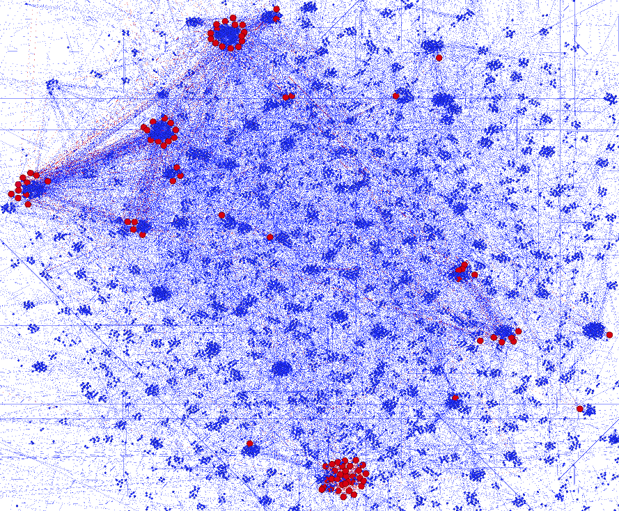
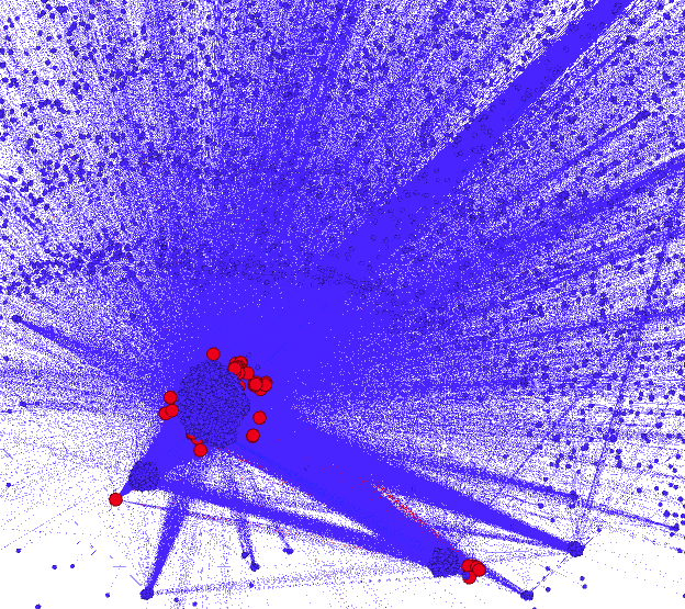
Figure 8: Clusters of High Attitude nodes

Spatial Proximity of Nodes with High attitude.  Finally we visualized the location of nodes with high attitude values (Figure 8). Red nodes are the nodes with high attitude. We used the clustering algorithm mentioned in  [6] to identify communities, and visualized them using the OpenOrd algorithm  [26] from Gephi  [5] which is used for visually distinguishing clusters. For graph Epinions, a total of 708 communities were identified. We we looked at the top 100 attitude nodes, we noticed that all these nodes were limited to only 5 of those communities. Similarly, for graph CA-HepTh, 473 communities were identified. The top 100 attitude nodes were limited to 12 of them. This behavior was observed in other graphs as well, which showed that high attitude nodes are generally restricted to a few communities rather than being distributed across the network.

VIII Conclusion

In this work we have formalized the notion of strength of influence/attitude in social networks and have formulated the attitude maximization problem. We present various theoretical properties related to our formulation. We also introduce the notion of actionable attitude to capture high attitude nodes by defining this quality as the (expected) difference between total attitude and the number of influenced nodes. There are several other ways to formulate this notion—for example, by looking at the ratio of attitude and influence or by examining the number of entities whose attitude value is above a threshold. Exploring these alternative formulations would be interesting.

References

• [1] Charu C. Aggarwal, Arijit Khan, and Xifeng Yan. On flow authority discovery in social networks. In Proceedings of SIAM International Conference on Data Mining, pages 522–533, 2011.
• [2] I. Ajzen. Nature and operation of attitudes. Annual Review of Psychology, 52:27–58, 2001.
• [3] A. Arora, S. Galhotra, and S. Ranu. Debunking the myths of influence maximization: An in-depth benchmarking study. In SIGMOD, pages 651–666, 2017.
• [4] N. Barbieri, F. Bonchi, and G. Manco. Topic-aware social influence propagation models. In ICDM, pages 81–90, 2012.
• [5] Mathieu Bastian, Sebastien Heymann, and Mathieu Jacomy. Gephi: An open source software for exploring and manipulating networks. 2009.
• [6] Vincent D Blondel, Jean-Loup Guillaume, Renaud Lambiotte, and Etienne Lefebvre. Fast unfolding of communities in large networks. Journal of Statistical Mechanics: Theory and Experiment, 2008(10):P10008, 2008.
• [7] C. Borgs, M. Brautbar, J. Chayes, and B. Lucier. Maximizing social influence in nearly optimal time. In SODA, pages 946–957, 2014.
• [8] S. Chen, J. Fan, G. Li, J. Feng, K-L. Tan, and J. Tang. Online topic-aware influence maximization. Proc. VLDB Endow., 8(6):666–677, 2015.
• [9] W. Chen, A. Collins, R. Cummings, T. Ke, Z. Liu, D. Rincón, X. Sun, Y. Wang, W. Wei, and Y. Yuan. Influence maximization in social networks when negative opinions may emerge and propagate. In SDM, pages 379–390, 2011.
• [10] W. Chen, C. Wang, and Y. Wang. Scalable influence maximization for prevalent viral marketing in large-scale social networks. In SIGKDD, pages 1029–1038, 2010.
• [11] P. Domingos and M. Richardson. Mining the network value of customers. In KDD, pages 57–56, 2001.
• [12] A. Duane and J. Scott. Understanding Change in Social Attitudes. 1996.
• [13] M. Fishbein and I. Ajzen. Belief, Attitude, Intention, and Behavior: An Introduction to Theory and Research. Addison-Wesley, 1975.
• [14] S. Galhotra, A. Arora, and S. Roy. Holistic influence maximization: Combining scalability and efficiency with opinion-aware models. In SIGMOD, pages 743–758, 2016.
• [15] J. Guo, P. Zhang, C. Zhou, Y. Cao, and L. Guo. Personalized influence maximization on social networks. In CIKM 13, pages 199–208, 2013.
• [16] Keke Huang, Sibo Wang, Glenn Bevilacqua, Xiaokui Xiao, and Laks V. S. Lakshmanan. Revisiting the stop-and-stare algorithms for influence maximization. Proc. VLDB Endow., 10(9):913–924, May 2017.
• [17] K. Jung, W. Heo, and W. Chen. IRIE: scalable and robust influence maximization in social networks. In ICDM 2012., pages 918–923, 2012.
• [18] D. Kempe, J. Kleinberg, and E. Tardos. Maximizing the spread of influence through a social network. In KDD, pages 137–146, 2003.
• [19] Andreas Krause, Ajit Singh, and Carlos Guestrin. Near-optimal sensor placements in gaussian processes: Theory, efficient algorithms and empirical studies. Journal of Machine Learning Research, 9(8):235–284, 2008.
• [20] J. Leskovec, A. Krause, C. Guestrin, C. Faloutsos, J. VanBriesen, and N. Glance. Cost-effective outbreak detection in networks. In KDD, pages 420–429, 2007.
• [21] F.H. Li, C.T. Li, and M.K. Shan. Labeled influence maximization in social networks for target marketing. In PASSAT/SocialCom 2011, pages 560–563, 2011.
• [22] Y. Li, D. Zhang, and K-L. Tan. Real-time targeted influence maximization for online advertisements. VLDB, 8(10):1070–1081, 2015.
• [23] Q. Liu, B. Xiang, L. Zhang, E. Chen, C. Tan, and J. Chen. Linear computation for independent social influence. In IEEE 13th International Conference on Data Mining, pages 468–477, 2013.
• [24] Qi Liu, Biao Xiang, Nicholas Jing Yuan, Enhong Chen, Hui Xiong, Yi Zheng, and Yu Yang. An influence propagation view of pagerank. ACM Transaction of Knowledge Discovery Data, 11(3), 2017.
• [25] W. Lu and L. V. S. Lakshmanan. Profit maximization over social networks. In ICDM, pages 479–488, 2012.
• [26] Shawn Martin, W Michael Brown, Richard Klavans, and Kevin Boyack. Openord: An open-source toolbox for large graph layout. Proc SPIE, 7868:786806, 01 2011.
• [27] George Nemhauser, Laurence Wolsey, and M L. Fisher. An analysis of approximations for maximizing submodular set functions. 14:265–294, 12 1978.
• [28] H. Nguyen, M. Thai, and T. Dinh. Stop-and-stare: Optimal sampling algorithms for viral marketing in billion-scale networks. In Proceedings SIGMOD, pages 695–710, 2016.
• [29] M. Padmanabhan, N. Somisetty, S. Basu, and A. Pavan. Influence maximization in social networks with non-target constraints. In IEEE International Conference on Big Data, Big Data 2018, pages 771–780, 2018.
• [30] M. Rokeach. Beliefs, Attitudes and Values. Jossey-Bass, 1970.
• [31] C. Song, W. Hsu, and M. L. Lee. Targeted influence maximization in social networks. In Proc. of CIKM 16, pages 1683–1692, 2016.
• [32] Y. Tang, Y. Shi, and X. Xiao. Influence maximization in near-linear time: A martingale approach. In SIGMOD, pages 1539–1554, 2015.
• [33] Y. Tang, X. Xiao, and Y. Shi. Influence maximization: near-optimal time complexity meets practical efficiency. In SIGMOD, pages 75–86, 2014.
• [34] R. Zajonc. Attitudinal effects of mere exposure. Journal of Personality and Social Psychology., 9(2):1–27, 1968.
• [35] H. Zhang, T. N. Dinh, and M. T. Thai. Maximizing the spread of positive influence in online social networks. In ICDCS, pages 317–326, 2013.
• [36] Chuan Zhou, Peng Zhang, Wenyu Zang, and Li Guo. Maximizing the cumulative influence through a social network when repeat activation exists. In International Conference on Computational Science, pages 422 – 431, 2014.