Notes on constructions of knots with the same trace

Abstract.

The $m$-trace of a knot is the $4$-manifold obtained from $\mathbf{B}^{4}$ by attaching a $2$-handle along the knot with $m$-framing. In 2015, Abe, Jong, Luecke and Osoinach introduced a technique to construct infinitely many knots with the same $m$-trace, which is called the operation $(\ast m)$. In this paper, we prove that their technique can be explained in terms of Gompf and Miyazaki’s dualizable pattern. In addition, we show that the family of knots admitting the same $4$-surgery given by Teragaito can be explained by the operation $(\ast m)$.

1. Introduction

For an integer $m$, the $m$-trace $X_{K}(m)$ of a knot $K$ is the $4$-manifold obtained from $\mathbf{B}^{4}$ by attaching a $2$-handle along the knot with $m$-framing. On techniques to construct knots with the same trace, the following are known.

• Abe, Jong, Luecke and Osoinach [2] introduced a technique to construct infinitely many knots with the same $m$-trace, which is based on “annulus presentation” and called the operation $(\ast m)$ (for annulus presentations and the operation $(\ast m)$, see Section 2).

• Miller and Piccirillo [7] constructed a pair of knots with the same $m$-trace by utilizing dualizable patterns (for dualizable patterns, see Section 3).

Miller and Piccirillo [7] explained the operation $(\ast m)$ in terms of dualizable patterns in the case $m=0$ by constructing a dualizable pattern from an annulus presentation with some condition.

In this paper, we proved that, for any $m\in\mathbf{Z}$, the operation $(\ast m)$ can be also explained in terms of dualizable patterns (Theorem 4.1). As an application, we directly draw the duals to Miller and Piccirillo’s dualizable patterns (Theorem 4.3 and Figure 5). In addition, we explain the family of knots admitting the same $4$-surgery given by Teragaito [10] in terms of the operation $(\ast m)$ (Section 5). We also some observations in the final section. Throughout this paper,

• unless specifically mentioned, all knots and links are smooth and unoriented, and all other manifolds are smooth and oriented,

• for an $n$-component link $L_{1}\cup\dots\cup L_{n}$, we denote the $3$-manifold obtained from $\mathbf{S}^{3}$ by $m_{i}$-surgery on a knot $L_{i}$ for any $i$ by $M_{L_{1}\cup\dots\cup L_{n}}(m_{1},\dots,m_{n})$,

• we denote a tubular neighborhood of a knot $K$ in a $3$-manifold by $\nu(K)$,

• we denote the unknot in $\mathbf{S}^{3}$ by $U$.

2. Annulus twist, annlus presentation and the operation $(\ast m)$

2.1. Annulus twist and annulus presentation

Let $A\subset\mathbf{S}^{3}$ be an embedded annulus with ordered boundaries $\partial A=c_{1}\cup c_{2}$. An $n$-fold annulus twist along $A$ is to apply $(lk(c_{1},c_{2})+1/n)$-surgery along $c_{1}$ and $(lk(c_{1},c_{2})-1/n)$-surgery along $c_{2}$, where we give $c_{1}$ and $c_{2}$ parallel orientations. We see that the resulting manifold obtained by an annulus twist is also $\mathbf{S}^{3}$.

Let $A\subset\mathbf{S}^{3}$ be an embedded annulus with $\partial A=c_{1}\cup c_{2}$. Take an embedding of a band $b\colon I\times I\rightarrow\mathbf{S}^{3}$ such that

• $b(I\times I)\cap\partial A=b(\partial I\times I)$,

• $b(I\times I)\cap\operatorname{Int}A$ consists of ribbon singularities, and

• $A\cup b(I\times I)$ is an immersion of an orientable surface,

where $I=[0,1]$. If a knot $K\subset\mathbf{S}^{3}$ is isotopic to the knot $(\partial A\setminus b(\partial I\times I))\cup b(I\times\partial I)$, then we call $(A,b)$ an annulus presentation of $K$. An annulus presentation $(A,b)$ is special if $A$ is unknotted and $\operatorname{lk}(c_{1},c_{2})=\pm 1$ (that is, $A$ is $\pm 1$-full twisted). Let $K$ be a knot with an annulus presentation $(A,b)$. Let $A^{\prime}\subset A$ be a shrunken annulus with $\partial A^{\prime}=c^{\prime}_{1}\cup c^{\prime}_{2}$ which satisfies the following:

• $\overline{A\setminus A^{\prime}}$ is a disjoint union of two annuli,

• each $c^{\prime}_{i}$ is isotopic to $c_{i}$ in $\overline{A\setminus A^{\prime}}$ for $i=1,2$ and

• $A\setminus(\partial A\cup A^{\prime})$ does not intersect $b(I\times I)$.

Then, by $A^{n}(K)$, we denote the knot obtained from $K$ by the $n$-fold annulus twist along $A^{\prime}$. For simplicity, we denote $A^{1}(K)$ by $A(K)$ and $A^{0}(K)$ by $K$.

Remark 2.1.

We find many examples of annulus presentations in [1, 2, 4, 9]. In this paper, for an annulus presentation $(A,b)$, we often draw the attaching regions $A\cap b$ by bold arcs and we omit the band $b$.

By utilizing Osoinach’s work [8, Theorem 2.3], for a knot $K$ with an annulus presentation $(A,b)$, we see that $M_{K}(0)$ and $M_{A^{n}(K)}(0)$ are orientation-preservingly homeomorphic for any $n\in\mathbf{Z}$. In particular, a homeomorphism $\phi_{n}\colon M_{K}(0)\rightarrow M_{A^{n}(K)}(0)$ is given as in Figure 1, which is explicitly given by Teragaito [10]. We call $\phi_{n}$ the $n$-th Osoinach-Teragaito’s homeomorphism. Moreover, if $(A,b)$ is special, by applying Abe, Jong, Omae and Takeuchi’s result [1, Theorem 2.8] to the knot, we see that the homeomorphism $\phi_{n}$ extends to an orientation-preserving diffeomorphism $\Phi_{n}\colon X_{K}(0)\rightarrow X_{A^{n}(K)}(0)$ for any $n\in\mathbf{Z}$.

As a consequence, we obtain the following.

Theorem 2.2.

Let $K\subset\mathbf{S}^{3}$ be a knot with an annulus presentation $(A,b)$. Then, there is an orientation-preservingly homeomorphism $\phi_{n}\colon M_{K}(0)\rightarrow M_{A^{n}(K)}(0)$ for any $n\in\mathbf{Z}$. In particular, $\phi_{n}$ is given as in Figure 1. Moreover, if $(A,b)$ is special, $\phi_{n}$ extends to an orientation-preserving diffeomorphism $\Phi_{n}\colon X_{K}(0)\rightarrow X_{A^{n}(K)}(0)$.

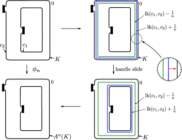
Figure 1. (color online) Osoinach-Teragaito’s homeomorphism $\phi_{n}$. For simplicity we draw $A$ as a flat annulus although $A$ may be knotted and twisted.

2.2. Operation $(\ast m)$

Let $K$ be a knot with a special annulus presentation $(A,b)$. Let $\gamma_{A(K)}\subset\mathbf{S}^{3}\setminus\nu(A(K))$ be a curve depicted in Figure 2. Remark that the definition of $\gamma_{A(K)}$ depends on the twist of $A$.

Figure 2. (color online) The curve $\gamma_{A(K)}$

Denote the knot obtained from $A(K)$ by twisting $m$ times along $\gamma_{A(K)}$ by $T_{m}(A(K))$. In [2, Section 3.1.2], the operation $K\mapsto T_{m}(A(K))$ is called the operation $(\ast m)$. Then, Abe, Jong, Luecke and Osoinach [2] proved the following theorem.

Theorem 2.3 ([2, Theorem 3.7 and Theorem 3.10]).

Let $K$ be a knot with a special annulus presentation $(A,b)$. Then, there is an orientation-preservingly homeomorphism $\psi_{m}\colon M_{K}(m)\rightarrow M_{T_{m}(A(K))}(m)$ which extends to a diffeomorphism $\Psi_{m}\colon X_{K}(m)\rightarrow X_{T_{m}(A(K))}(m)$ for any $m\in\mathbf{Z}$.

Concretely, $\psi_{m}$ is given as in Figure 3 for the case $A$ is $+1$ twisted. Similarly, we also obtain $\psi_{m}$ for the case $A$ is $-1$ twisted.

Remark 2.4.

Note that Osoinach-Teragaito’s homeomorphism induces a homeomorphism $\phi_{+1}\colon(M_{K}(0),\alpha_{K})\rightarrow(M_{A(K)}(0),\gamma_{A(K)})$, where $\alpha_{K}\subset\mathbf{S}^{3}\setminus\nu(K)$ is a meridian of $K$ and we regard $\alpha_{K}$ and $\gamma_{A(K)}$ as curves in $M_{K}(0)$ and $M_{A(K)}(0)$ (see also the bottom arrow in Figure 3).

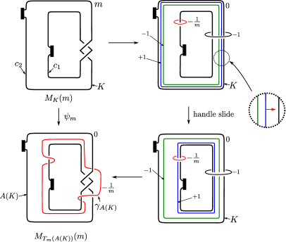
Figure 3. (color online) The homeomorphism $\psi_{m}\colon M_{K}(m)\rightarrow M_{T_{m}(A(K))}(m)$ for the case $A$ is $+1$ twisted. For the case $A$ is $-1$ twisted, we define $\psi_{m}$ by the same way.

3. Relation between annulus presentation and dualizable pattern

3.1. Dualizable pattern

Here, we recall the definition of dualizable patterns, which is firstly given by Gompf and Miyazaki [6] and developed by Miller and Piccirillo [7] (see also [9]).

Let $P\colon\mathbf{S}^{1}\rightarrow V$ be an oriented knot in a solid torus $V=\mathbf{S}^{1}\times D^{2}$. Suppose that the image $P(\mathbf{S}^{1})$ is not null-homologous in $V$. Such a $P$ is called a pattern. By an abuse of notation, we use the notation $P$ for both a map and its image. Define $\lambda_{V}$, $\mu_{P}$, $\mu_{V}$ and $\lambda_{P}$ as follows:

• put $\lambda_{V}=\mathbf{S}^{1}\times\{x_{0}\}\subset\partial V\subset V$ for some $x_{0}\in\partial D^{2}$ and orient $\lambda_{V}$ so that $P$ is homologous to $r\lambda_{V}$ in $V$ for some positive $r\in\mathbf{Z}_{>0}$,

• define $\mu_{P}\subset V$ by a meridian of $P$ and orient $\mu_{P}$ so that the linking number of $P$ and $\mu_{P}$ is $1$,

• put $\mu_{V}=\{x_{1}\}\times\partial D^{2}\subset\partial V\subset V$ for some $x_{1}\in\mathbf{S}^{1}$ and orient $\mu_{V}$ so that $\mu_{V}$ is homologous to $s\mu_{P}$ in $V\setminus\nu(P)$ for some positive $s\in\mathbf{Z}_{>0}$,

• define $\lambda_{P}$ by a longitude of $P$ which is homologous to $t\lambda_{V}$ in $V\setminus\nu(P)$ for some positive $t\in\mathbf{Z}_{>0}$.

For an oriented knot $K\subset\mathbf{S}^{3}$, let $\iota_{K}\colon V\rightarrow\mathbf{S}^{3}$ be an embedding which identifies $V$ with $\overline{\nu(K)}$ and sends $\lambda_{V}$ to an oriented curve on $\partial\overline{\nu(K)}$ which is null-homologous in $\mathbf{S}^{3}\setminus\nu(K)$ and isotopic to $K$ in $\mathbf{S}^{3}$. Then $\iota_{K}\circ P\colon\mathbf{S}^{1}\rightarrow\mathbf{S}^{3}$ represents an oriented knot. The knot is called the satellite of $K$ with pattern $P$ and denoted by $P(K)$.

A pattern $P\colon\mathbf{S}^{1}\rightarrow V$ is dualizable if there is a pattern $P^{\ast}\colon\mathbf{S}^{1}\rightarrow V^{\ast}$ and an orientation-preserving homeomorphism $f\colon V\setminus\nu(P)\rightarrow V^{\ast}\setminus\nu(P^{\ast})$ such that $f(\lambda_{V})=\lambda_{P^{\ast}}$, $f(\lambda_{P})=\lambda_{V^{\ast}}$, $f(\mu_{V})=-\mu_{P^{\ast}}$ and $f(\mu_{P})=-\mu_{V^{\ast}}$.

Miller and Piccirillo [7, Proposition 2.5] introduced a convenient technique to determine whether a given pattern is dualizable as follows (see also [6, Section 2]). Define $\Gamma\colon\mathbf{S}^{1}\times D^{2}\rightarrow\mathbf{S}^{1}\times\mathbf{S}^{2}$ by $\Gamma(t,d)=(t,\gamma(d))$, where $\gamma\colon D^{2}\rightarrow\mathbf{S}^{2}$ is an arbitrary orientation preserving embedding. For any curve $c\colon\mathbf{S}^{1}\rightarrow\mathbf{S}^{1}\times D^{2}$, define $\widehat{c}=\Gamma\circ c\colon\mathbf{S}^{1}\rightarrow\mathbf{S}^{1}\times\mathbf{S}^{2}$. Then, we obtain the following proposition.

Proposition 3.1 ([7, Proposition 2.5]).

A pattern $P$ in a solid torus $V$ is dualizable if and only if $\widehat{P}$ is isotopic to $\widehat{\lambda_{V}}$ in $\mathbf{S}^{1}\times\mathbf{S}^{2}$.

Related to knot traces, the following are known. Let $P\subset V$ be a pattern. Let $\tau_{m}\colon V\rightarrow V$ be a homeomorphism given by twisting $m$ times along a meridian of $V$. It is known that if $P$ is dualizable then $\tau_{m}(P)$ is also dualizable and its dual is given by $\tau_{-m}(P^{\ast})$, where $P^{\ast}$ is the dual to $P$ (see [7, Theorem 3.6] and [9, Remark 4.6]). Moreover, we obtain the following.

Theorem 3.2 ([7, Theorem 3.6] and [9, Remark 4.6]).

Let $P$ be a dualizable pattern and $P^{\ast}$ be its dual. Then, we have $X_{P(U)}(m)\cong X_{\tau_{m}(P^{\ast})(U)}(m)$ for any $m\in\mathbf{Z}$.

Remark 3.3.

For a dualizable pattern $P\subset V$, we see that $M_{P(U)\cup\mu_{V}}(0,0)\cong\mathbf{S}^{3}$. Conversely, for a link $k\cup c$ with $M_{k\cup c}(0,0)\cong\mathbf{S}^{3}$, we see that $k\subset\mathbf{S}^{3}\setminus\nu(c)$ is a dualizable pattern after giving some orientation to $k$ (for detail, see [5] and [9, Remarks 3.3 and 4.6]).

3.2. From special annulus presentations to dualizable patterns

In this section, we recall Miller and Piccirillo’s construction ([7, Section 5]) of dualizable patterns from a special annulus presentation (see also [9]).

Let $K\subset\mathbf{S}^{3}$ be a knot with a special annulus presentation $(A,b)$. In Figure 4, the left knots represent $K$, and each right knot represents $A^{\pm 1}(K)$ for the corresponding left $K$. Then, for each case, take curves $\beta_{K}^{\pm}\subset\mathbf{S}^{3}\setminus\nu(K)$ as in Figure 4.

Let $P_{+}$ (resp. $P_{-}$) be the pattern given by $K\subset V_{+}=\mathbf{S}^{3}\setminus\nu(\beta_{K}^{+})$ (resp. $K\subset V_{-}=\mathbf{S}^{3}\setminus\nu(\beta_{K}^{-})$), where we give a parameter of $V_{\pm}$ so that $P_{\pm}(U)=K$. Moreover, we give an orientation of $P_{\pm}$ arbitrarily. Then, we can check that $P_{\pm}$ are dualizable patterns (for example, slide $K$ along the $0$-framing of $\beta_{K}^{\pm}$ in $M_{\beta_{K}^{\pm}}(0)\cong\mathbf{S}^{1}\times\mathbf{S}^{2}$ and apply Proposition 3.1). These dualizable patterns satisfy the following.

Proposition 3.4 (e.g. [7, Proposition 5.3] and [9, Proposition 3.9]).

Let $K$ be a knot with a special annulus presentation $(A,b)$. Let $P_{+}$ and $P_{-}$ be the dualizable patterns as above. Then we have $P_{\pm}(U)=K$ and $P_{\pm}^{\ast}(U)=A^{\pm 1}(K)$.

Remark 3.5.

The homeomorphisms given in Figure 1 induces homeomorphisms

$$\phi_{\pm 1}\colon(M_{K}(0),\beta_{K}^{\pm})\rightarrow(M_{A^{\pm 1}(K)}(0),\alpha_{A^{\pm 1}(K)}),$$

where $\alpha_{A^{\pm 1}(K)}\subset\mathbf{S}^{3}\setminus\nu(A^{\pm 1}(K))$ is a meridian of $A^{\pm 1}(K)$. Here we regard $\beta_{K}^{\pm}$ and $\alpha_{A^{\pm 1}(K)}$ as curves in $M_{K}(0)$ and $M_{A^{\pm 1}(K)}(0)$ under the identifications

$$\mathbf{S}^{3}\setminus\nu(K) \cong M_{K}(0)\setminus\nu(L_{K}),$$

$$\mathbf{S}^{3}\setminus\nu(A^{\pm 1}(K)) \cong M_{A^{\pm 1}(K)}(0)\setminus\nu(L_{A^{\pm 1}(K)}),$$

respectively, where $L_{K}$ and $L_{A^{\pm 1}(K)}$ are the corresponding surgery duals.

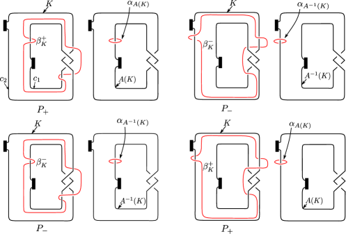
Figure 4. (color online) From a special annulus presentation $(A,b)$ of a knot $K$ to dualizable patterns $P_{+}$ and $P_{-}$ given by $K\subset\mathbf{S}^{3}\setminus\nu(\beta_{K}^{\pm})=V_{\pm}$

4. Operation $(\ast m)$ and dualizable pattern

By Theorems 2.3 and 3.2, for a knot $K$ with a special annulus presentation $(A,b)$, we have

$$X_{\tau_{m}(P_{+}^{\ast})(U)}(m)\cong X_{P_{+}(U)}(m)=X_{K}(m)\cong X_{T_{m}(A(K))}(m),$$

where $P_{+}$ is the dualizable pattern obtained from $K$ as in Section 3.2. Hence, it is a natural question whether $\tau_{m}(P_{+}^{\ast})(U)$ is isotopic to $T_{m}(A(K))$ or not. Proposition 3.4 implies that the answer is “yes” if $m=0$. The following theorem gives the affirmative answer to this question for any $m\in\mathbf{Z}$.

Theorem 4.1.

Let $K$ be a knot with a special annulus presentation $(A,b)$. Let $P_{+}$ be the dualizable pattern obtained from $K$ as in Section 3.2. Then, we obtain $\tau_{m}(P_{+}^{\ast})(U)=T_{m}(A(K))$ for any $m\in\mathbf{Z}$.

Miller and Piccirillo [7, Proposition 5.3] proved Theorem 4.1 for $m=0$. We can prove Theorem 4.1 by extending Miller and Piccirillo’s proof as follows.

Proof.

Let $L_{T_{m}(A(K))}^{(m)}\subset M_{T_{m}(A(K))}(m)$ be the surgery dual to $T_{m}(A(K))$. Let $\alpha_{T_{m}(A(K))}\subset\mathbf{S}^{3}\setminus\nu(T_{m}(A(K)))$ be a meridian of $T_{m}(A(K))$. Then, we can regard $\alpha_{T_{m}(A(K))}$ as a curve in $M_{T_{m}(A(K))}(m)$ by using the following identification

(1) $$\mathbf{S}^{3}\setminus\nu(T_{m}(A(K)))=M_{T_{m}(A(K))}(m)\setminus\nu(L_{T_{m}(A(K))}^{(m)}).$$

Since $\alpha_{T_{m}(A(K))}$ is isotopic to $L_{T_{m}(A(K))}^{(m)}$ in $M_{T_{m}(A(K))}(m)$, we have

(2) $$M_{T_{m}(A(K))}(m)\setminus\nu(L_{T_{m}(A(K))}^{(m)})\cong M_{T_{m}(A(K))}(m)\setminus\nu(\alpha_{T_{m}(A(K))}).$$

Let $\beta_{K}^{+}\subset\mathbf{S}^{3}\setminus\nu(K)$ be the curve given in Section 3.2 (see also Figure 4). We can also regard $\beta_{K}^{+}$ as a curve in $M_{K}(m)$ under the identification $\mathbf{S}^{3}\setminus\nu(K)\cong M_{K}(m)\setminus\nu(L_{K}^{(m)})$, where $L_{K}^{(m)}$ is the surgery dual to $K$. Then, we can check that $\psi_{m}(\beta_{K}^{+})=\alpha_{T_{m}(A(K))}$, where $\psi_{m}\colon M_{K}(m)\rightarrow M_{T_{m}(A(K))}(m)$ is given in Figure 3. Hence, we obtain

(3) $$M_{T_{m}(A(K))}(m)\setminus\nu(\alpha_{T_{m}(A(K))}) \cong M_{K}(m)\setminus\nu(\beta_{K}^{+})$$

$$\cong M_{K\cup\alpha_{K}}(0,-1/m)\setminus\nu(\beta_{K}^{+})$$

$$\cong\mathbf{S}^{3}\setminus\nu(K\cup\alpha_{K}\cup\beta_{K}^{+})\cup\bigsqcup_{i=0,1}(S_{i}^{1}\times D_{i}^{2}),$$

where the last (small) union is given by identifying $\partial D_{0}^{2}$ with $0$-framing of $K$ and $\partial D_{1}^{2}$ with $-1/m$-framing of $\alpha_{K}$.

Recall that the solid torus $V_{+}$ containing $P_{+}$ is given by $V_{+}=\mathbf{S}^{3}\setminus\nu(\beta_{K}^{+})$. Since, the $0$-framing of $K$ is viewed as $\lambda_{P_{+}}$ and $\alpha_{K}$ is viewed as $\mu_{P_{+}}$ in $V_{+}$, we have

(4) $$\mathbf{S}^{3}\setminus\nu(K\cup\alpha_{K}\cup\beta_{K}^{+})\cup\bigsqcup_{i=0,1}(S_{i}^{1}\times D_{i}^{2})$$

$$\cong((V_{+}\setminus\nu(P_{+}))\setminus\nu(\mu_{P_{+}}))\cup\bigsqcup_{i=0,1}(S_{i}^{1}\times D_{i}^{2}),$$

where the last (small) union is given by identifying $\partial D_{0}^{2}$ with $\lambda_{P_{+}}$ and $\partial D_{1}^{2}$ with $-1/m$-framing of $\mu_{P_{+}}$. By the dualizability of $P_{+}$, we obtain

(5) $$((V_{+}\setminus\nu(P_{+}))\setminus\nu(\mu_{P_{+}}))\cup\bigsqcup_{i=0,1}(S_{i}^{1}\times D_{i}^{2})$$

$$\cong((V_{+}^{\ast}\setminus\nu(P^{\ast}_{+}))\setminus\nu(\mu_{V^{\ast}_{+}}))\cup\bigsqcup_{i=0,1}(S_{i}^{1}\times D_{i}^{2})$$

$$\cong(V_{+}^{\ast}\setminus\nu(\tau_{m}(P^{\ast}_{+})))\cup(S_{0}^{1}\times D_{0}^{2})$$

$$\cong\mathbf{S}^{3}\setminus\nu(\tau_{m}(P^{\ast}_{+})(U)),$$

where the last union is given by identifying $\partial D_{0}^{2}$ with $\lambda_{V_{+}^{\ast}}$. By (1)–(5) and the Knot Complement Theorem, we obtain $\tau_{m}(P_{+}^{\ast})(U)=T_{m}(A(K))$. ∎

Remark 4.2.

Let $K$ be a knot with a special annulus presentation $(A,b)$. Let $\overline{K}$ be the mirror image of $K$ and $(\overline{A},\overline{b})$ be the special annulus presentation of $\overline{K}$ obtained from $(A,b)$ by taking mirror image. Let $\gamma_{A^{-1}(K)}\subset\mathbf{S}^{3}\setminus\nu(A^{-1}(K))$ be the mirror image of $\gamma_{\overline{A}(\overline{K})}\subset\mathbf{S}^{3}\setminus\nu(\overline{A}(\overline{K}))$ (see also Figure 5). Denote the knot obtained from $A^{-1}(K)$ by twisting $m$ times along $\gamma_{A^{-1}(K)}$ by $T_{m}(A^{-1}(K))$. Then, by the similar discussion to Theorem 4.1, we see that $\tau_{m}(P^{\ast}_{-})(U)=T_{m}(A^{-1}(K))$ for any $m\in\mathbf{Z}$.

We see that $A(K)\subset\mathbf{S}^{3}\setminus\nu(\gamma_{A(K)})=V^{\prime}_{+}$ also gives a dualizable pattern, where the parameter of $V^{\prime}_{+}\cong\mathbf{S}^{1}\times D^{2}$ is given by the standard way. Denote it by $P_{+}^{\prime}$. It is easy to see that $\tau_{m}(P_{+}^{\prime})(U)=T_{m}(A(K))=\tau_{m}(P_{+}^{\ast})(U)$ for any $m\in\mathbf{Z}$. So we can consider the question which asks whether $P^{\prime}_{+}$ is equal to $P_{+}^{\ast}$ as a pattern. We can give the affirmative answer to the question as follows.

Theorem 4.3.

Let $K$ be a knot with a special annulus presentation $(A,b)$. Let $P_{+}^{\prime}\subset V^{\prime}_{+}$ be the dualizable pattern as above, and let $P_{+}^{\ast}\subset V^{\ast}_{+}$ be the dualizable pattern obtained from $K$ as in Section 3.2. Then, for any $m\in\mathbf{Z}$, there is an orientation-preserving homeomorphism $h\colon V^{\prime}_{+}\rightarrow V^{\ast}_{+}$ such that

• $h(\tau_{m}(P^{\prime}_{+}))=\tau_{m}(P_{+}^{\ast})$,

• $h(\lambda_{V^{\prime}_{+}})=\lambda_{V^{\ast}_{+}}$ and $h(\mu_{V^{\prime}_{+}})=\mu_{V^{\ast}_{+}}$.

Namely, $P^{\prime}_{+}=P^{\ast}_{+}$ as patterns.

Proof.

By the definition of the operation $(\ast m)$, we see that

(6) $$M_{T_{m}(A(K))}(m)\setminus\nu(\alpha_{T_{m}(A(K))})$$

$$\cong M_{A(K)\cup\gamma_{A(K)}}(0,-1/m)\setminus\nu(\alpha_{A(K)})$$

$$\cong\mathbf{S}^{3}\setminus\nu(A(K)\cup\gamma_{A(K)}\cup\alpha_{A(K)})\cup\bigsqcup_{i=0,1}(S_{i}^{1}\times D_{i}^{2}),$$

where the last (small) union is given by identifying $\partial D_{0}^{2}$ with $0$-framing of $A(K)$ and $\partial D_{1}^{2}$ with $-1/m$-framing of $\gamma_{(A(K))}$. Since $\alpha_{A(K)}$ is isotopic to the surgery dual to $A(K)$, we have

(7) $$\mathbf{S}^{3}\setminus\nu(A(K)\cup\gamma_{A(K)}\cup\alpha_{A(K)})\cup\bigsqcup_{i=0,1}(S_{i}^{1}\times D_{i}^{2})$$

$$\cong\mathbf{S}^{3}\setminus\nu(A(K)\cup\gamma_{A(K)})\cup(S_{1}^{1}\times D_{1}^{2})$$

$$=(V^{\prime}_{+}\setminus\nu(\tau_{m}(P_{+}^{\prime})))\cup(S_{2}^{1}\times D_{2}^{2}),$$

where the last union is given by identifying $\partial D_{2}^{2}$ with $\lambda_{V^{\prime}_{+}}$. By considering the composition of (7), (6), (3), (4) and (5) we obtain an orientation-preserving homeomorphism

$$\overline{h}\colon(V_{+}^{\prime}\setminus\nu(\tau_{m}(P_{+}^{\prime})))\cup(S_{2}^{1}\times D_{2}^{2})\rightarrow(V^{\ast}_{+}\setminus\nu(\tau_{m}(P^{\ast}_{+})))\cup(S_{0}^{1}\times D_{0}^{2}).$$

Then, we can check that

• $\overline{h}(\lambda_{\tau_{m}(P^{\prime}_{+})})=\lambda_{\tau_{m}(P_{+}^{\ast})}$,

• $\overline{h}(\lambda_{V^{\prime}_{+}})=\lambda_{V^{\ast}_{+}}$ and $\overline{h}(\mu_{V^{\prime}_{+}})=\mu_{V^{\ast}_{+}}$,

• $\overline{h}(S_{2}^{1}\times D_{2}^{2})=S_{0}^{1}\times D_{0}^{2}$.

Hence, $\overline{h}$ induces a desired homeomorphism. ∎

Remark 4.4.

Similarly, we can define $P^{\prime}_{-}$ as $A^{-1}(K)\subset\mathbf{S}^{3}\setminus\nu(\gamma_{A^{-1}(K)})=V^{\prime}_{-}$ (see also Remark 4.2). By the same discussion as the proof of Theorem 4.3, we see that there is an orientation-preserving homeomorphism $h\colon V^{\prime}_{-}\rightarrow V^{\ast}_{-}$ which satisfies $h(\tau_{m}(P^{\prime}_{-}))=\tau_{m}(P_{-}^{\ast})$, $h(\lambda_{V^{\prime}_{-}})=\lambda_{V^{\ast}_{-}}$ and $h(\mu_{V^{\prime}_{-}})=\mu_{V^{\ast}_{-}}$.

Remark 4.5.

We see that Theorem 4.3 induces Theorem 4.1 since $\tau_{m}(P_{+}^{\ast})(U)=\tau_{m}(P_{+}^{\prime})(U)$ by Theorem 4.3 and $\tau_{m}(P_{+}^{\prime})(U)=T_{m}(A(K))$ by the definition of $P^{\prime}_{+}$.

By Theorem 4.3 and Remark 4.4, we can draw the duals $P^{\ast}_{\pm}$ to $P_{\pm}$ as in Figure 5, where $P_{\pm}$ are the dualizable patterns obtained from a knot $K$ with a special annulus presentation $(A,b)$ as in Section 3.2.

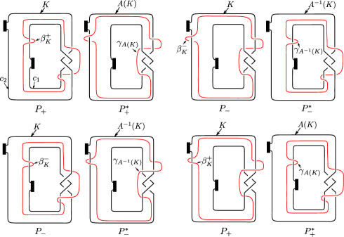
Figure 5. (color online) The dualizable patterns $P_{\pm}\subset V_{\pm}=\mathbf{S}^{3}\setminus\nu(\beta_{K}^{\pm})$ and $P_{\pm}^{\ast}\subset V_{\pm}^{\ast}=\mathbf{S}^{3}\setminus\nu(\gamma_{A^{\pm 1}(K)})$

5. Flipped annulus twist and operation $(\ast\pm 4)$

In [10], Teragaito gave the first example of a Seifert fibered manifold which is represented by the same integral surgery on infinitely many hyperbolic knots. In the work, Teragaito used a presentation of $9_{42}$, which is almost the same as a special annulus presentation but does not satisfy the last condition: $A\cup b$ is an immersion of an orientable surface. Teragaito explained that, for a knot with such a presentation, we obtain a family of knots admitting the same $4$-surgery (not $0$-surgery) by annulus twists along (a shrunken annulus of) the annulus. It has been known that such knots have the same $4$-trace (see [1, Theorem 2.8]).

In this section, we prove that the above phenomenon can be explained in terms of the operation $(\ast 4)$.

5.1. Flipped annulus twist

Let $A\subset\mathbf{S}^{3}$ be an embedded annulus with ordered boundary $\partial A=c_{1}\cup c_{2}$. We suppose that $A$ is unknottend and $\operatorname{lk}(c_{1},c_{2})=\pm 1$, where we give $c_{1}$ and $c_{2}$ parallel orientations. Then, an $n$-fold flipped annulus twist along $A$ is to apply $(-lk(c_{1},c_{2})+1/n)$-surgery along $c_{1}$ and $(-lk(c_{1},c_{2})-1/n)$-surgery along $c_{2}$ (compare with Section 2.1).

Let $K$ be a knot with a special annulus presentation $(A,b)$. Then, by $A_{f}^{n}(K)$, we denote the knot obtained from $K$ by the $n$-fold flipped annulus twist along $A^{\prime}$, where $A^{\prime}$ is a shrunken annulus given in Section 2.1. For simplicity, we also denote $A_{f}^{1}(K)$ by $A_{f}(K)$. We also see $A_{f}^{n}(K)$ as follows: After “flipping” $c_{1}$ (or $c_{2}$) as in Figure 6, we find another annulus $A_{f}$. Then, by using [3, Lemma 7.15], we see that $A_{f}^{n}(K)$ is obtained from $K$ by applying the $n$-fold annulus twist along $A^{\prime}_{f}$, where $A^{\prime}_{f}$ is a shrunken annulus of $A_{f}$. Remark that $(A_{f},b)$ is not an annulus presentation any more since $A_{f}\cup b$ is an immersion of a non-orientable surface.

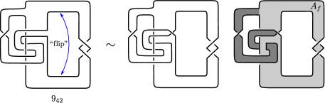
Figure 6. (color online) An annulus presentation of $9_{42}$ (left). After “flipping” $c_{1}$, we find a new annulus $A_{f}$.

5.2. Relation to the operation $(\ast\pm 4)$

Teragaito [10, Proposition 2.1] proved that there is an orientation-preserving homeomorphism $M_{K}(r)\rightarrow M_{A^{n}_{f}(K)}(r)$, where $r=-4\operatorname{lk}(c_{1},c_{2})\in\{\pm 4\}.$ Denote this homeomorphism by

$$\phi_{n}^{f}\colon M_{K}(r)\rightarrow M_{A^{n}_{f}(K)}(r).$$

For a sketch of the proof, see Figure 7. Then, we notice that

(8) $$\phi_{\pm 1}^{f}(\beta^{\mp}_{K})=\alpha_{A^{\pm 1}_{f}(K)},$$

where $\alpha_{A^{\pm 1}_{f}(K)}$ is a meridian of $A^{\pm 1}_{f}(K)$ and we regard $\beta^{\pm}_{K}$ and $\alpha_{A^{\pm 1}_{f}(K)}$ as curves in $M_{K}(r)$ and $M_{A^{n}_{f}(K)}(r)$, respectively (by using the same discussion in Remark 3.5). We have seen that $M_{T_{r}(A(K))}(r)\cong M_{K}(r)\cong M_{A^{-1}_{f}(K)}(r)$. Moreover, we can prove that

(9) $$T_{r}(A^{\mp 1}(K))=A^{\pm 1}_{f}(K).$$

In fact, by replacing $\psi_{m}$ with $\phi_{\pm 1}^{f}$ and $\beta_{K}^{+}$ with $\beta_{K}^{\mp}$ in the proof of Theorem 4.1, we see that $\mathbf{S}^{3}\setminus\nu(A_{f}^{\pm 1}(K))\cong\mathbf{S}^{3}\setminus\nu(\tau_{r}(P^{\ast}_{\mp})(U))\cong\mathbf{S}^{3}\setminus\nu(T_{r}(A^{\mp 1}(K))).$ By the Knot Complement Theorem, we obtain Equation (9). As a consequence, we obtain the following.

Theorem 5.1.

Let $K$ be a knot with a special annulus presentation $(A,b)$ with $\partial A=c_{1}\cup c_{2}$. Then we obtain

$$T_{r}(A^{\mp 1}(K))=A^{\pm 1}_{f}(K),$$

where $r=-4\operatorname{lk}(c_{1},c_{2})$, and we give $c_{1}$ and $c_{2}$ parallel orientations.

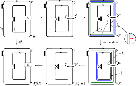
Figure 7. (color online) . The homeomorphism $\phi_{n}^{f}\colon M_{K}(r)\rightarrow M_{A^{n}_{f}(K)}(r)$, where $\varepsilon\in\{\pm 1\}$ and $r=-4\varepsilon$. The box with $\varepsilon$ represents $\varepsilon$-full-twist. For convenience, we draw an orientation of the knot (not $c_{1}$ and $c_{2}$).

Remark 5.2.

In private communication, Tetsuya Abe commented that $T_{4}(A(9_{42}))$ and $A^{-1}_{f}(9_{42})$ may be equivalent because of computational calculations. Theorem 5.1 is inspired by the comment.

6. Discussions

6.1. Naturality

Let $K$ be a knot with a special annulus presentation $(A,b)$. Then, we obtain a dualizable pattern $P_{+}$ as in Section 3.2. Put $\check{K}=A(K)$ and give the natural annulus presentation $(\check{A},\check{b})$ of $\check{K}$ from $(A,b)$. Then we obtain another dualizable pattern $\check{P}_{-}$ from $\check{K}$ as in Section 3.2. We see that these patterns satisfy $P_{+}(U)=K$, $P_{+}^{\ast}(U)=A(K)$, $\check{P}_{-}(U)=A(K)$ and $\check{P}_{-}^{\ast}(U)=K$. More strongly, Theorem 4.3 and Figure 5 imply that $P_{+}=\check{P}_{-}^{\ast}$ and $P_{+}^{\ast}=\check{P}_{-}$.

Let $SAP$ be the set of special annulus presentations and $DP$ be the set of unoriented patterns which are dualizable after giving some orientation. Then, by the above discussion, we obtain the following commutative diagram:

$$\begin{CD}SAP@>{\pm}>{}>DP\\ @V{A^{\pm 1}}V{}V@V{}V{\ast}V\\ SAP@>{\mp}>{}>DP\end{CD}$$

where

• $A^{\pm 1}\colon SAP\rightarrow SAP$ is the map induced by $\pm 1$-fold annulus twist,

• $\pm\colon SAP\rightarrow DP$ is given by $(A,b)\mapsto P_{\pm}$ as in Section 3.2 and

• $\ast\colon DP\rightarrow DP$ is given by $P\mapsto P^{\ast}$.

6.2. Generalization

For more general setting, we obtain the following result by the proof of Theorem 4.1. Remark that, in Theorem 6.1 below, we regard curves $\beta$ and $\alpha_{K_{2}}$ as curves in $M_{K_{1}}(m)$ and $M_{K_{2}}(m)$, respectively, under the identification $\mathbf{S}^{3}\setminus\nu(K_{i})=M_{K_{i}}(m)\setminus\nu(L_{K_{i}})$, where $L_{K_{i}}$ is the surgery dual.

Theorem 6.1.

Let $K_{1}$ and $K_{2}$ be knots in $\mathbf{S}^{3}$. Let $\beta\subset\mathbf{S}^{3}\setminus\nu(K_{1})$ be an unknot. Let $\alpha_{K_{2}}\subset\mathbf{S}^{3}\setminus\nu(K_{2})$ be a meridian of $K_{2}$. Suppose that $P=K_{1}\subset\mathbf{S}^{3}\setminus\nu(\beta)$ gives a dualizable pattern. Then, if there is an orientation-preserving homeomorphism $\phi\colon M_{K_{1}}(m)\rightarrow M_{K_{2}}(m)$ such that $\phi(\beta)=\alpha_{K_{2}}$, we have $\tau_{m}(P^{\ast})(U)=K_{2}$. Moreover $\phi$ extends to a diffeomorphism $\Phi\colon X_{K_{1}}(m)\rightarrow X_{K_{2}}(m)$.

The last claim follows from the same discussion as Theorem 3.2.

Question 6.2.

Let $\phi\colon M_{K_{1}}(m)\rightarrow M_{K_{2}}(m)$ be an orientation-preserving homeomorphism. Then, when is there an unknot $\beta\subset\mathbf{S}^{3}\setminus\nu(K_{1})$ which satisfies the condition of Theorem 6.1? Moreover, if exists, is such $\beta$ unique up to isotopy in $\mathbf{S}^{3}\setminus\nu(K_{1})$?

Acknowledgements. The author was supported by JSPS KAKENHI Grant number JP18K13416.

References

- [1] T. Abe, I. Jong, Y. Omae, and M. Takeuchi, Annulus twist and diffeomorphic 4-manifolds, Math. Proc. Cambridge Philos. Soc. 155 (2013), no. 2, 219–235. MR 3091516
- [2] T. Abe, I. D. Jong, J. Luecke, and J. Osoinach, Infinitely many knots admitting the same integer surgery and a four-dimensional extension, Int. Math. Res. Not. IMRN (2015), no. 22, 11667–11693. MR 3456699
- [3] T. Abe and K. Tagami, Knot with infinitely many non-characterizing slopes, arXiv:2003.07163v1.
- [4] T. Abe and K. Tagami, Fibered knots with the same 0-surgery and the slice-ribbon conjecture, Math. Res. Lett. 23 (2016), no. 2, 303–323. MR 3512887
- [5] K. Baker and K. Motegi, Noncharacterizing slopes for hyperbolic knots, Algebr. Geom. Topol. 18 (2018), no. 3, 1461–1480. MR 3784010
- [6] R. E. Gompf and K. Miyazaki, Some well-disguised ribbon knots, Topology Appl. 64 (1995), no. 2, 117–131. MR 1340864
- [7] A. N. Miller and L. Piccirillo, Knot traces and concordance, J. Topol. 11 (2018), no. 1, 201–220. MR 3784230
- [8] J. Osoinach, Manifolds obtained by surgery on an infinite number of knots in , Topology 45 (2006), no. 4, 725–733. MR 2236375
- [9] K. Tagami, On annulus presentations, dualizable patterns and RGB-diagrams, submitted.
- [10] M. Teragaito, A Seifert fibered manifold with infinitely many knot-surgery descriptions, Int. Math. Res. Not. IMRN (2007), no. 9, Art. ID rnm 028, 16. MR 2347296