On annulus presentations, dualizable patterns and RGB-diagrams

Abstract.

The $0$-trace of a knot is the $4$-manifold represented by the $0$-framing of the knot. In this manuscript, we survey methods constructing a pair of knots with diffeomorphic $0$-traces. In particular, we focus on Gompf-Miyazaki’s dualizable pattern, Abe-Jong-Omae-Takeuchi’s band presentation, and RGB-diagram given by Piccirillo and named by the author, and we draw the relations among these methods directly. As an application, we give a sufficient condition that two knots obtained by Abe-Jong-Omae-Takeuchi’s method coincide.

1. Introduction

A knot in $\mathbf{S}^{3}=\partial\mathbf{B}^{4}$ is smoothly slice if it bounds a proper and smooth disk in $\mathbf{B}^{4}$. We can find many motivations to study the smooth sliceness of knots, for example:

• If the smooth $4$-dimensional Poincaré conjecture is true, then for two knots $K$ and $K^{\prime}$ having homeomorphic $0$-surgeries $K$ is smoothly slice if and only if $K^{\prime}$ is smoothly slice ([1, Lemma 3.2]).

• It is conjectured that any smoothly slice knot is a ribbon knot (Slice-Ribbon Conjecture) [7].

The $0$-trace of a knot is the $4$-manifold obtained from $\mathbf{B}^{4}$ by attaching a $2$-handle along the $0$-framing of the knot. The following theorem (Theorem 1.1) implies that the $0$-trace of a knot has the complete information to determine whether the knot is smoothly slice or not.

Theorem 1.1.

A knot is smoothly slice if and only if its $0$-trace smoothly embeds in $\mathbf{S}^{4}$.

Akbulut and Kirby [12, Problem 1.19] conjectured that two knots having homeomorphic $0$-surgeries are concordant. As mentioned above, if one of the two knots is smoothly slice, this conjecture is true under the smooth $4$-dimensional Poincaré conjecture. However, it has been proved that this conjecture is false. In fact, Yasui [22] gave infinitely many counterexamples for Akbulut-Kirby’s conjecture.

Gompf and Miyazaki [9, Proposition 3.1] gave a pair of knots which have homeomorphic $0$-surgeries and whose connected sum is not ribbon by utilizing a pattern, which is called a dualizable pattern in this manuscript (for definition, see Section 3). In particular, there is no ribbon concordance between them in both directions. Abe and the author [3] also gave such a pair of knots. In [3], we use the technique called “annulus twist” and “annulus presentation”, which are essentially given by Osoinach [15] and improved in [20, 1]. By utilizing [1, Theorem 2.8], we see that Abe and the author’s knots have diffeomorphic $0$-traces. We also see that Gompf and Miyazaki’s knots have diffeomorphic $0$-traces by [14, Theorem 3.1]. Hence, we can consider the following question:

Are two knots having diffeomorphic $0$-traces concordant?

This question has been negatively solved by Miller and Piccirillo [14]. In fact, they gave infinitely many pairs of knots such that they have diffeomorphic $0$-traces and yet are distinct in smooth concordance by using dualizable patterns. They also mentioned a relation between annulus presentations and dualizable patterns.

Recently, Piccirillo [16] introduced a class of Kirby diagrams $R\cup G\cup B$. In this manuscript, we call a Kirby diagram of the class an RGB-diagram (for definition, see Section 4). As an application, Piccirillo [17] constructed a non-slice knot whose $0$-trace is diffeomorphic to that of the Conway knot. In particular, we see that the Conway knot is not smoothly slice by Theorem 1.1. We remark that Piccirillo’s construction can be explained in terms of annulus presentations and annulus twists (see Remark 4.11).

In this manuscript, we survey annulus presentations, dualizable patterns and RGB-diagrams, and we draw an RGB-diagram from an annulus presentation explicitly. In particular, we clarify the relation among “special” annulus presentations (defined in Section 2), dualizable patterns and RGB-diagrams (see Theorems 4.8 and Figure 1). Moreover, we extend this relation to the oriented case (Theorem 4.9). As an application, we give a sufficient condition for a knot with an annulus presentation to be preserved under the corresponding annulus twist (Theorem 5.1).

Figure 1. Relations among special annulus presentations, dualizable patterns and RGB-diagrams. (i) is given by Miller-Piccirillo [14, Section 5]. (ii) and its inverse are given by Piccirillo [16, Proposition 4.2]. (iii) is given in Theorem 4.8. The inverses of (i) and (iii) do not exist (Remark 4.10). These relations can be extended to oriented versions (see Sections 3.3 and 4.2, and Theorem 4.9).

1.1. Notation

Throughout this manuscript,

• we denote the $3$-manifold obtained from $\mathbf{S}^{3}$ by applying $n$-framed surgery on a knot $K\subset\mathbf{S}^{3}$ by $M_{K}(n)$,

• the $n$-trace of a knot $K$ is the $4$-manifold obtained from $\mathbf{B}^{4}$ by attaching a $2$-handle along an $n$-framed knot $K\subset\mathbf{S}^{3}$ and we denote it by $X_{K}(n)$,

• we denote an open regular neighborhood of a submanifold $P$ in a manifold $V$ by $\nu(P)$,

• we denote the unknot in $\mathbf{S}^{3}$ by $U$,

• unless specifically mentioned, all knots and links are smooth and unoriented, and all other manifolds are smooth and oriented,

• for a manifold $M$, define $-M$ to be the manifold obtained by reversing the orientation,

• for a Kirby diagram $L$, we denote the $4$-manifold that $L$ represents by $X_{L}$, and

• we will use $\cong$ to denote orientation-preservingly differomorphic $4$-manifolds or homeomorphic $3$-manifolds.

2. Annulus presentation

2.1. Annulus twist

Let $A\subset\mathbf{S}^{3}$ be an embedded annulus with $\partial A=c_{1}\cup c_{2}$. An $n$-fold annulus twist along $A$ is to apply $(\operatorname{lk}(c_{1},c_{2})+1/n)$-surgery on $c_{1}$ and $(\operatorname{lk}(c_{1},c_{2})-1/n)$-surgery on $c_{2}$, where $\operatorname{lk}(c_{1},c_{2})$ is the linking number of $c_{1}$ and $c_{2}$, and we give $c_{1}$ and $c_{2}$ parallel orientations. We see that the resulting manifold obtained by an annulus twist is $\mathbf{S}^{3}$.

2.2. Annulus presentation

Let $A\subset\mathbf{S}^{3}$ be an embedded annulus with $\partial A=c_{1}\cup c_{2}$. Take an embedding of a band $b\colon I\times I\rightarrow\mathbf{S}^{3}$ such that

• $b(I\times I)\cap\partial A=b(\partial I\times I)$,

• $b(I\times I)\cap\operatorname{Int}A$ consists of ribbon singularities, and

• $A\cup b(I\times I)$ is an immersion of an orientable surface,

where $I=[0,1]$. If a knot $K\subset\mathbf{S}^{3}$ is isotopic to the knot $(\partial A\setminus b(\partial I\times I))\cup b(I\times\partial I)$, then we call $(A,b)$ an annulus presentation of $K$. An annulus presentation $(A,b)$ is special if $A$ is a Hopf band.

Remark 2.1.

In the definition of special annulus presentations, if we omit the condition that $A\cup b(I\times I)$ is an immersion of an orientable surface, it coincides with the definition of band presentations defined by Abe, Jong, Omae and Takeuchi [1]. In particular, a special annulus presentation is a band presentation. Note that in [2, 4], our special annulus presentations are called “annulus presentations”.

Example 2.2.

The knot $6_{3}$ has a special annulus presentation $(A,b)$ (Figure 2).

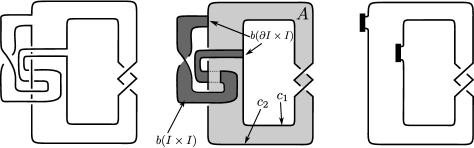
Figure 2. A special annulus presentation of $6_{3}$. For simplicity, we often draw an annulus presentation as the right picture, where the attaching regions for the band are represented by bold arcs and the bands are omitted.

Let $K$ be a knot with an annulus presentation $(A,b)$. Let $\widetilde{A}\subset A$ be a shrunken annulus with $\partial\widetilde{A}=\widetilde{c}_{1}\cup\widetilde{c}_{2}$ which satisfies the following:

• $\overline{A\setminus\widetilde{A}}$ is a disjoint union of two annuli,

• each $\widetilde{c}_{i}$ is isotopic to $c_{i}$ in $\overline{A\setminus\widetilde{A}}$ for $i=1,2$, and

• $A\setminus(\partial A\cup\widetilde{A})$ does not intersect $b(I\times I)$.

Then, by $A^{n}(K)$, we denote the knot obtained from $K$ by the $n$-fold annulus twist along $\widetilde{A}$. For simplicity, we also use $A(K)$ instead of $A^{1}(K)$.

Example 2.3.

We consider the knot $6_{3}$ with the annulus presentation $(A,b)$ in Figure 2. Then $A(6_{3})$ is the right picture in Figure 3.

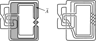
Figure 3. A shrunken annulus $\tilde{A}$ for an annulus presentation of $6_{3}$ (left) and $A(6_{3})$ (right).

The following theorem is essentially due to Osoinach [15, Theorem 2.3].

Theorem 2.4.

Let $K\subset\mathbf{S}^{3}$ be a knot with an annulus presentation $(A,b)$. Then, for any $n\in\mathbf{Z}$ there is an orientation-preservingly homeomorphism $\phi_{n}\colon M_{K}(0)\rightarrow M_{A^{n}(K)}(0)$.

The homeomorphism $\phi_{n}$ in Theorem 2.4 is concretely given by Figure 4 (see also [20]).

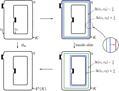
Figure 4. (color online) Homeomorphism $\phi_{n}$. In this picture the annulus $A$ may be knotted and twisted.

Abe, Jong, Omae and Takeuchi [1, Theorem 2.8] partially extended Theorem 2.4. In particular, by applying their result to a knot with a special annulus presentation, we obtain the following.

Theorem 2.5.

Let $K\subset\mathbf{S}^{3}$ be a knot with a special annulus presentation $(A,b)$. Then, the homeomorphism $\phi_{n}\colon M_{K}(0)\rightarrow M_{A^{n}(K)}(0)$ given by Figure 4 extends to an orientation-preservingly diffeomorphism $\Phi_{n}\colon X_{K}(0)\rightarrow X_{A^{n}(K)}$ for any $n\in\mathbf{Z}$.

3. Dualizable pattern

In this section, we recall the definition of dualizable patterns. For details on dualizable patterns, see [9] and [14].

3.1. Dualizable pattern

Let $P\colon\mathbf{S}^{1}\rightarrow V$ be an oriented knot in a solid torus $V=\mathbf{S}^{1}\times D^{2}$. Such a $P$ is called a pattern. By an abuse of notation, we use the notation $P$ for both a map and its image. Suppose that the image $P(\mathbf{S}^{1})$ is not null-homologous in $V$. Define $\lambda_{V}$, $\mu_{P}$, $\mu_{V}$ and $\lambda_{P}$ as follows:

• put $\lambda_{V}=\mathbf{S}^{1}\times\{x_{0}\}\subset\partial V\subset V$ for some $x_{0}\in\partial D^{2}$ and orient $\lambda_{V}$ so that $P$ is homologous to $k\lambda_{V}$ in $V$ for some positive $k\in\mathbf{Z}_{>0}$,

• define $\mu_{P}\subset V$ by a meridian of $P$ and orient $\mu_{P}$ so that the linking number of $P$ and $\mu_{P}$ is $1$,

• put $\mu_{V}=\{x_{1}\}\times\partial D^{2}\subset\partial V\subset V$ for some $x_{1}\in\mathbf{S}^{1}$ and orient $\mu_{V}$ so that $\mu_{V}$ is homologous to $l\mu_{P}$ in $V\setminus\nu(P)$ for some positive $l\in\mathbf{Z}_{>0}$, and

• define $\lambda_{P}$ by a longitude of $P$ which is homologous to $m\lambda_{V}$ in $V\setminus\nu(P)$ for some positive $m\in\mathbf{Z}_{>0}$.

For an oriented knot $K\subset\mathbf{S}^{3}$, let $\iota_{K}\colon V\rightarrow\mathbf{S}^{3}$ be an embedding which identifies $V$ with $\overline{\nu(K)}$ and sends $\lambda_{V}$ to the $0$-framing of $K$. Then $\iota_{K}\circ P\colon\mathbf{S}^{1}\rightarrow\mathbf{S}^{3}$ represents an oriented knot. The knot is called the satellite of $K$ with pattern $P$ and denoted by $P(K)$.

A pattern $P\colon\mathbf{S}^{1}\rightarrow V$ is dualizable if there is a pattern $P^{\ast}\colon\mathbf{S}^{1}\rightarrow V^{\ast}$ and an orientation-preserving homeomorphism $f\colon V\setminus\nu(P)\rightarrow V^{\ast}\setminus\nu(P^{\ast})$ such that $f(\lambda_{V})=\lambda_{P^{\ast}}$, $f(\lambda_{P})=\lambda_{V^{\ast}}$, $f(\mu_{V})=-\mu_{P^{\ast}}$ and $f(\mu_{P})=-\mu_{V^{\ast}}$. We call $P^{\ast}$ the dual of $P$.

Miller and Piccirillo [14, Proposition 2.5] introduced a convenient technique to determine whether a given pattern is dualizable as follows (see also [9, Section 2]). Define $\Gamma\colon\mathbf{S}^{1}\times D^{2}\rightarrow\mathbf{S}^{1}\times\mathbf{S}^{2}$ by $\Gamma(t,d)=(t,\gamma(d))$, where $\gamma\colon D^{2}\rightarrow\mathbf{S}^{2}$ is an arbitrary orientation-preserving embedding. For any curve $c\colon\mathbf{S}^{1}\rightarrow\mathbf{S}^{1}\times D^{2}$, define $\widehat{c}=\Gamma\circ c\colon\mathbf{S}^{1}\rightarrow\mathbf{S}^{1}\times\mathbf{S}^{2}$. Then, we obtain the following proposition.

Proposition 3.1 ([14, Proposition 2.5]).

A pattern $P$ in a solid torus $V$ is dualizable if and only if $\widehat{P}$ is isotopic to $\widehat{\lambda_{V}}$ in $\mathbf{S}^{1}\times\mathbf{S}^{2}$.

Proof.

For the sake of completeness, we introduce the proof due to Miller and Piccirillo. Suppose that $\widehat{P}$ is isotopic to $\widehat{\lambda_{V}}$ in $\mathbf{S}^{1}\times\mathbf{S}^{2}$. Then, $V^{\ast}=\mathbf{S}^{1}\times\mathbf{S}^{2}\setminus\nu(\widehat{P})\cong\mathbf{S}^{1}\times\mathbf{S}^{2}\setminus\nu(\widehat{\lambda_{V}})$ is a solid torus. We identify $V^{\ast}$ with $\mathbf{S}^{1}\times D^{2}$ so that $\widehat{\lambda_{P}}\subset V^{\ast}$ is identified with $\lambda_{V^{\ast}}=\mathbf{S}^{1}\times\{x_{0}\}$ for some $x_{0}\in D^{2}$. Define a pattern $Q$ by $\widehat{\lambda_{V}}\subset V^{\ast}$. Note that the orientation of $\widehat{\lambda_{V}}$ is determined by that of $\widehat{P}$. Since $\mathbf{S}^{1}\times\mathbf{S}^{2}\setminus\nu(\widehat{\lambda_{V}})\cong V$, we have

$$V\setminus\nu(P)\cong\mathbf{S}^{1}\times\mathbf{S}^{2}\setminus\nu(\widehat{P}\cup\widehat{Q})\cong V^{\ast}\setminus\nu(Q).$$

This induces an orientation-preserving homeomorphism $f\colon V\setminus\nu(P)\rightarrow V^{\ast}\setminus\nu(Q)$ such that $f(\lambda_{V})=\lambda_{Q}$, $f(\lambda_{P})=\lambda_{V^{\ast}}$, $f(\mu_{V})=-\mu_{Q}$ and $f(\mu_{P})=-\mu_{V^{\ast}}$. Hence, we have $P^{\ast}=Q$.

Conversely, suppose that a pattern $P$ in a solid torus $V$ is dualizable. Then, there is an orientation-preserving homeomorphism $f\colon V\setminus\nu(P)\rightarrow V^{\ast}\setminus\nu(P^{\ast})$ such that $f(\lambda_{V})=\lambda_{P^{\ast}}$, $f(\lambda_{P})=\lambda_{V^{\ast}}$, $f(\mu_{V})=-\mu_{P^{\ast}}$ and $f(\mu_{P})=-\mu_{V^{\ast}}$. Let $V_{1}$ be a solid torus and $\mu_{V_{1}}$ be a meridian of $V_{1}$. Then, we have

$$\mathbf{S}^{1}\times\mathbf{S}^{2}\setminus\nu(\widehat{P}) \cong(V\setminus\nu(P))\cup_{\partial}V_{1}$$

$$\cong(f(V\setminus\nu(P)))\cup_{\partial}V_{1}$$

$$=(V^{\ast}\setminus\nu(P^{\ast}))\cup_{\partial}V_{1}$$

$$=V^{\ast},$$

where the first union is given by identifying $\mu_{V}$ with $\mu_{V_{1}}$, and the second and the third unions are given by identifying $-\mu_{P^{\ast}}$ with $\mu_{V_{1}}$. Hence, $\widehat{P}$ is a knot in $\mathbf{S}^{1}\times\mathbf{S}^{2}$ whose complement is a solid torus. By Waldhausen [21], it is proved that all genus one Heegaard splittings of $\mathbf{S}^{1}\times\mathbf{S}^{2}$ are isotopic. Hence, $\widehat{P}$ is isotopic to $\pm\widehat{\lambda_{V}}$. Here, by the definition of $\lambda_{V}$, $P$ is homologous to a $m\lambda_{V}$ in $V\setminus\nu(P)$ for some positive $m\in\mathbf{Z}_{>0}$, and we see that $\widehat{P}$ is isotopic to $+\widehat{\lambda_{V}}$. ∎

By Proposition 3.1, we can draw the dual $P^{\ast}$ for a given dualizable pattern $P$ as in Figure 5 (see also [9, Section 4] and [14, Figure 2]).

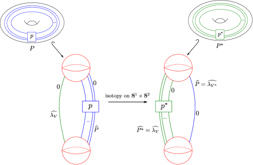
Figure 5. (color online) A dualizable pattern $P$ and its dual $P^{\ast}$. The pairs of two balls represent $\mathbf{S}^{1}\times\mathbf{S}^{2}$. To clarify the parameters of the tori $V=\mathbf{S}^{1}\times\mathbf{S}^{2}\setminus\nu(\widehat{\lambda_{V}})$ and $V^{\ast}=\mathbf{S}^{1}\times\mathbf{S}^{2}\setminus\nu(\widehat{P})$, we draw the $0$-framings of $\widehat{\lambda_{V}}$ and $\widehat{\lambda_{V^{\ast}}}$.

Remark 3.2.

Miller and Piccirillo [14] commented that Waldhausen [21] only proved the uniqueness of the genus one Heegaard splitting of $\mathbf{S}^{1}\times\mathbf{S}^{2}$ up to differmorphism and we require more work to prove the uniqueness up to isotopy. For a complete proof, for example, we use the following two facts (see also [6]).

• For any orientable surface $F$, every Heegaard splitting of $F\times\mathbf{S}^{1}$ is a stabilization of the standard one [18].

• Two stabilizations with the same genus of the same Heegaard splitting are isotopic (for example, see [11]). Namely, a stabilization of a Heegaard splitting is uniquely defined.

Remark 3.3.

Baker and Motegi [5] gave another description of dualizable pattern as follows. Let $k\cup c$ be a two-component link in $\mathbf{S}^{3}$ such that $c$ is the unknot and that the $(0,0)$-surgery on $k\cup c$ results in $\mathbf{S}^{3}$. In the proof of [5, Lemma 2.3], Baker and Motegi proved that $k$ is isotopic to an $\mathbf{S}^{1}$-fiber in the standard product structure of $M_{c}(0)\cong\mathbf{S}^{1}\times\mathbf{S}^{2}$ by utilizing Gabai’s work [8, Corollary 8.3]. In particular, $k$ is isotopic to a meridian of $c$ in $M_{c}(0)$. By Proposition 3.1, we see that $k\subset\mathbf{S}^{3}\setminus\nu(c)\cong\mathbf{S}^{1}\times D^{2}$ represents a dualizable pattern. Moreover, if we give the solid torus $\mathbf{S}^{3}\setminus\nu(c)\cong\mathbf{S}^{1}\times D^{2}$ a parameter in a standard way so that $k(U)=k$, then for the dual $k^{\ast}$, we see that $k^{\ast}(U)$ is the surgery dual to $c$ in the surgered $\mathbf{S}^{3}$. Conversely, let $P\colon\mathbf{S}^{1}\rightarrow V$ be a dualizable pattern and $\mu_{V}$ be a meridian of $V$. We regard $V$ as a standard solid torus in $\mathbf{S}^{3}$. Then the two-component link $P\cup\mu_{V}$ in $\mathbf{S}^{3}$ satisfies $M_{P\cup\mu(V)}(0,0)\cong\mathbf{S}^{3}$ since $\widehat{P}$ is isotopic to $\widehat{\lambda_{V}}$ in $M_{\mu_{V}}(0)\cong\mathbf{S}^{1}\times\mathbf{S}^{2}$.

Remark 3.4.

Let $P$ be a pattern. Then, $P$ is homologous to $m\lambda_{V}$ for some non-negative $m\in\mathbf{Z}$ in $V$. We call $m$ the algebraic winding number of $P$. The geometric winding number of $P$ is the minimal number of intersections between a meridian disk of $V$ and a pattern which is isotopic to $P$ in $V$. By Proposition 3.1, we see that

• any geometric winding number one pattern is dualizable and its dual is itself (see Figure 6, and see also [9, Figure 2] and [5, Lemma 2.4]).

• the algebraic winding number of any dualizable pattern is one (see Figure 7).

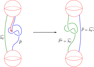
Figure 6. (color online) The left picture is $\widehat{P}$ for a geometric winding number one pattern $P$. The pairs of two balls represent $\mathbf{S}^{1}\times\mathbf{S}^{2}$.

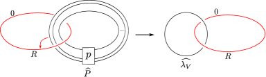
Figure 7. (color online) A dualizable pattern $P$, and $\widehat{P}$. In this picture, $\mathbf{S}^{1}\times\mathbf{S}^{2}$ is represented by a knot $R$ with $0$-framing. Since $P$ is dualizable, $\widehat{P}$ is isotopic to $\widehat{\lambda_{V}}$ in $\mathbf{S}^{1}\times\mathbf{S}^{2}$. Such an isotopy is realized by isotopy on $\mathbf{S}^{3}$ and slidings over $R$. So, the algebraic winding number of $P$ is equal to the linking number of $R$ and $\widehat{\lambda_{V}}$.

The following theorem is the most basic property of dualizable patterns.

Theorem 3.5 (e.g. [9, Lemma 2.2] and [14, Theorem 2.8]).

If a pattern $P$ is dualizable, then there is an orientation-preserving homeomorphism $\phi\colon M_{P(U)}(0)\rightarrow M_{P^{\ast}(U)}(0)$.

Miller and Piccirillo [14] extended Theorem 3.5 as follows.

Theorem 3.6 (e.g.[14, Theorem 3.1]).

Let $P$ be a dualizable pattern. Then the homeomorphism $\phi\colon M_{P(U)}(0)\rightarrow M_{P^{\ast}(U)}(0)$ in Theorem 3.5 extends to an orientation-preserving diffeomorphism $\Phi\colon X_{P(U)}(0)\rightarrow X_{P^{\ast}(U)}(0)$.

3.2. From special annulus presentations to dualizable patterns

Miller and Piccirillo [14, Section 5] constructed a dualizable pattern from a special annulus presentation. Here, we introduce their construction.

Let $K\subset\mathbf{S}^{3}$ be a knot with a special annulus presentation $(A,b)$ with $\partial A=c_{1}\cup c_{2}$. Recall that $A$ is a Hopf band since $(A,b)$ is special. Now, we consider the knot $A^{\pm 1}(K)$. In Figures 8 and 9, the left blue knots represent $K$, and each right black knot represents $A^{\pm 1}(K)$ for the corresponding left $K$. More precisely,

• in Figure 8 $(1)$, $A$ is $-1$ twisted and the black knot is $A(K)$,

• in Figure 8 $(2)$, $A$ is $-1$ twisted and the black knot is $A^{-1}(K)$,

• in Figure 9 $(3)$, $A$ is $+1$ twisted and the black knot is $A^{-1}(K)$,

• in Figure 9 $(4)$, $A$ is $+1$ twisted and the black knot is $A(K)$,

for each left $K$. Then, for each case, take a red curve $\beta\subset\mathbf{S}^{3}\setminus\nu(K)$ as in Figures 8 and 9.

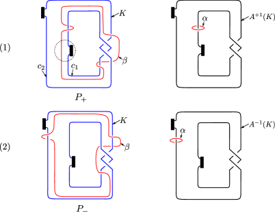
Figure 8. (color online) From a special annulus presentation $(A,b)$ of a knot $K$ (the left blue knots) to dualizable patterns $P_{+}$ (top) and $P_{-}$ (bottom) given by $K\subset\mathbf{S}^{3}\setminus\nu(\beta)$. Here, the Hopf band $A$ is $-1$ twisted. The red curves $\beta$ run near $c_{1}$ for $(1)$ and near $c_{2}$ for $(2)$. Precisely, for $(1)$, there is a sufficiently thin annulus bounded by $\beta$ and $c_{1}$ such that the thin annulus does not intersect the band $b$ except the attaching regions and the thin annulus is on $A$ near the attaching region on $c_{1}$ (circled by the dotted circle). The right black knots represent $A^{+1}(K)$ for $(1)$ and $A^{-1}(K)$ for $(2)$.

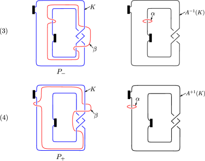
Figure 9. (continuation of Figure 8) Here, the Hopf band $A$ is $+1$ twisted. The red curves $\beta$ run near $c_{1}$ for $(3)$ and near $c_{2}$ for $(4)$. The right black knots represent $A^{-1}(K)$ for $(3)$ and $A^{+1}(K)$ for $(4)$.

Note that the homeomorphism given in Figure 4 induces a homeomorphism $\phi_{\pm 1}\colon(M_{K}(0),\beta)\rightarrow(M_{A^{\pm 1}(K)}(0),\alpha)$, where $\alpha\subset\mathbf{S}^{3}\setminus\nu(A^{\pm 1}(K))$ is a meridian of $A^{\pm 1}(K)$ and we regard $\beta$ and $\alpha$ as curves in $M_{K}(0)$ and $M_{A^{\pm 1}(K)}(0)$, respectively. Note also that $V=\mathbf{S}^{3}\setminus\nu(\beta)$ is homeomorphic to a solid torus. Let $P_{\pm}$ be the pattern given by $K\subset V$ as the left pictures of $A^{\pm 1}(K)$ in Figures 8 and 9, where we give a parameter of $V$ by regarding $V$ as a solid torus in a standard way so that $P_{\pm}(U)=K$. We give an orientation of $P_{\pm}$ arbitrarily. Then, we can prove that the patterns $P_{\pm}\subset V$ are dualizable as follows. Here, we only consider the case of Figure 8 $(1)$. Similarly, for other three cases, we can prove that the patterns are dualizable. Firstly, draw $\widehat{P_{+}}$ in $M_{\beta}(0)=\mathbf{S}^{1}\times\mathbf{S}^{2}$ as in the first picture of Figure 10. Secondly, slide $\widehat{P_{+}}$ over the $0$-framed knot $\beta$ along the black arrow in the first picture of Figure 10. Then, we see that $\widehat{P_{+}}$ is isotopic to $\widehat{\lambda_{V}}$ in $M_{\beta}(0)$. Hence, by Proposition 3.1, $P_{+}$ is dualizable and its dual $P_{+}^{\ast}$ is presented by the green curve $\widehat{\lambda_{V}}$ in $V^{\ast}=M_{\beta}(0)\setminus\nu(\widehat{P}_{+})$ in Figure 10.

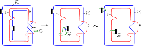
Figure 10. (color online) By sliding $\widehat{P_{+}}$ over the $0$-framed knot $\beta$ (red curve) along the black arrow (in the left picture), we see that $\widehat{P_{+}}$ is isotopic to $\widehat{\lambda_{V}}$ in $\mathbf{S}^{1}\times\mathbf{S}^{3}$ (right picture).

Obviously, $P_{\pm}(U)=K$ (as unoriented knots) . Miller and Piccirillo’s proof [14, Section 5] implies that $P_{+}^{\ast}(U)=A^{+1}(K)$ and $P_{-}^{\ast}(U)=A^{-1}(K)$ (as unoriented knots). For the sake of completeness, we introduce the proof.

As mentioned above, there is an orientation-preserving homeomorphism

$$\phi_{\pm 1}\colon(M_{K}(0),\beta)\rightarrow(M_{A^{\pm 1}(K)}(0),\alpha).$$

Let $L\subset M_{A^{\pm 1}(K)}(0)$ be the surgery dual to $A^{\pm 1}(K)$. Since $\alpha$ is isotopic to $L$ in $M_{A^{\pm 1}(K)}(0)$, we have

(1) $$\mathbf{S}^{3}\setminus\nu(A^{\pm 1}(K)) \cong M_{A^{\pm 1}(K)}(0)\setminus\nu(L)$$

$$\cong M_{A^{\pm 1}(K)}(0)\setminus\nu(\alpha)$$

$$\cong\phi_{\pm 1}^{-1}(M_{A^{\pm 1}(K)}(0))\setminus\phi_{\pm 1}^{-1}(\nu(\alpha))$$

$$=M_{K}(0)\setminus\nu(\beta)$$

$$\cong((\mathbf{S}^{3}\setminus\nu(\beta))\setminus\nu(P_{\pm}))\cup_{\partial}(\mathbf{S}^{1}\times D^{2}),$$

where the last union is given by identifying the $\lambda_{P_{\pm}}$ with a meridian of $\mathbf{S}^{1}\times D^{2}$. Recall that $V=\mathbf{S}^{3}\setminus\nu(\beta)$. Moreover, since $P_{\pm}$ is dualizable there is an orientation-preserving homeomorphism $f\colon V\setminus\nu(P_{\pm})\rightarrow V^{\ast}\setminus\nu(P_{\pm}^{\ast})$ such that $f(\lambda_{P_{\pm}})=\lambda_{V^{\ast}}$. Hence we obtain

(2) $$\mathbf{S}^{3}\setminus\nu(A^{\pm 1}(K)) \cong((\mathbf{S}^{3}\setminus\nu(\beta))\setminus\nu(P_{\pm}))\cup_{\partial}(\mathbf{S}^{1}\times D^{2})$$

$$=(V\setminus\nu(P_{\pm}))\cup_{\partial}(\mathbf{S}^{1}\times D^{2})$$

$$\cong(V^{\ast}\setminus\nu(P_{\pm}^{\ast}))\cup_{\partial}(\mathbf{S}^{1}\times D^{2})$$

$$\cong\mathbf{S}^{3}\setminus\nu(P_{\pm}^{\ast}(U)),$$

where the last union is given by identifying $\lambda_{V^{\ast}}$ with a meridian of $\mathbf{S}^{1}\times D^{2}$. Finally, by the Knot Complement Theorem [10], we see that $A^{\pm 1}(K)=P_{\pm}^{\ast}(U)$. As a consequence, we obtain Proposition 3.7.

Proposition 3.7 (e.g. [14, Proposition 5.3]).

Let $K$ be a knot with a special annulus presentation $(A,b)$. Then, there are dualizable patterns $P_{+}$ and $P_{-}$ such that $P_{\pm}(U)=K$ and $P_{\pm}^{\ast}(U)=A^{\pm 1}(K)$. In particular, such $P_{\pm}$ are drawn as in Figures 8 and 9.

In [19], the author gave the explicit formula of $P^{\ast}_{\pm}$ for the dualizable pattern $P_{\pm}$ in Proposition 3.7.

By Proposition 3.7, we can regard Theorem 3.6 as an extension of Theorem 2.5.

3.3. Oriented case

Let $K$ be an oriented knot with a special annulus presentation $(A,b)$. The orientation of $K$ induces orientations of $A^{\pm 1}(K)$ naturally. We can also give the orientations induced by $K$ to the dualizable patterns $P_{\pm}$ constructed from $K$ as in Section 3.2 (see also Figures 8 and 9). Moreover, their duals $P^{\ast}_{\pm}$ are also oriented by the orientations of $P_{\pm}$. Then, we can check that $P^{\ast}_{\pm}(U)=-A^{\pm 1}(K)$ as oriented knots as follows. Let $l$ be a longitude of $A^{\pm 1}(K)$ with $\operatorname{lk}(l,A^{\pm 1}(K))=0$. For convenience, orient $\beta$ depicted in Figures 8 and 9 so that $\operatorname{lk}(\beta,K)=1$. Let $\mu_{\beta}$ be a meridian of $\beta$ and orient $\mu_{\beta}$ so that $\operatorname{lk}(\beta,\mu_{\beta})=1$. Then, we see that the composition of homeomorphisms $\mathbf{S}^{3}\setminus\nu(A^{\pm 1}(K))\cong M_{A^{\pm 1}(K)}(0)\setminus\nu(\alpha)\cong M_{K}(0)\setminus\nu(\beta)$ given in Equation (1) sends $l$ to $\lambda_{P_{\pm}}-\mu_{\beta}$ (see Figure 11). Here, $\lambda_{P_{\pm}}$ bounds a disk in $M_{K}(0)\setminus\nu(\beta)$, and $\mu_{\beta}$ is $\lambda_{V}$ under the identification $V=\mathbf{S}^{3}\setminus\nu(\beta)$. Hence, $l$ is sent to $-\lambda_{V}$. Moreover, the homeomorphism $(V\setminus\nu(P_{\pm}))\cup_{\partial}(\mathbf{S}^{1}\times D^{2})\cong(V^{\ast}\setminus\nu(P_{\pm}^{\ast}))\cup_{\partial}(\mathbf{S}^{1}\times D^{2})$ in Equation (2) sends $\lambda_{V}$ to $\lambda_{P_{\pm}^{\ast}}$. As a consequence, $l$ is sent to a longitude of $P_{\pm}^{\ast}(U)$ with reversed orientation under the homeomorphism $\mathbf{S}^{3}\setminus\nu(A^{\pm 1}(K))\cong\mathbf{S}^{3}\setminus\nu(P_{\pm}^{\ast}(U))$ in Equation (2), and we obtain the following.

Proposition 3.8 (the oriented version of Proposition 3.7).

Let $K$ be an oriented knot with a special annulus presentation $(A,b)$. Give $A^{\pm 1}(K)$ the orientation induced by $K$. Then, there are dualizable patterns $P_{+}$ and $P_{-}$ such that $P_{\pm}(U)=K$ and $P_{\pm}^{\ast}(U)=-A^{\pm 1}(K)$ as oriented knots. In particular, such $P_{\pm}$ are drawn as in Figures 8 and 9, where the orientations of $P_{\pm}$ are induced by $K$ naturally.

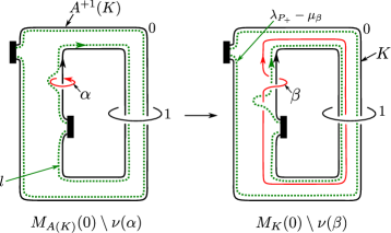
Figure 11. (color online) A longitude $l$ of $A(K)$ in $\mathbf{S}^{3}\setminus\nu(A(K))\cong M_{A(K)}(0)\setminus\nu(\alpha)$ (the dotted green loop in the left). Here, we consider the case $A$ is $-1$ twisted. The longitude $l$ is sent to $\lambda_{P_{+}}-\mu_{\beta}$ under the homeomorphism $\mathbf{S}^{3}\setminus\nu(A^{\pm 1}(K))\cong M_{K}(0)\setminus\nu(\beta)$.

4. Piccirillo’s RGB-diagram

In this section, we recall Piccirillo’s work [16] and describe a relation between the work and a special annulus presentation.

4.1. RGB-diagram

Let $L$ be a Kirby diagram which consists of one $1$-handle $R$ represented by a dotted unknotted circle and two $2$-handles $G$ and $B$ represented by $0$-framed knots. Suppose that $R$, $G$ and $B$ satisfying the following:

• $G\cup R$ is isotopic to $G\cup\mu_{G}$ in $\mathbf{S}^{3}$, where $\mu_{G}$ is a meridian of $G$,

• $B\cup R$ is isotopic to $B\cup\mu_{B}$ in $\mathbf{S}^{3}$, where $\mu_{B}$ is a meridian of $B$, and

• the linking number $\operatorname{lk}(G,B)$ of $G$ and $B$ is zero.

Then, we call $L$ an RGB-diagram. For example, see the bottom right picture in Figure 22 and [16] where $R$, $G$ and $B$ are drawn as red, green and blue curves, respectively. For an RGB-diagram $L=R\cup G\cup B$, we can construct two knots $K_{G}$ and $K_{B}$ as follows. Let $D_{R}$ be a disk bounded by $R$. Since $G\cup R$ is isotopic to $G\cup\mu_{G}$ in $\mathbf{S}^{3}$, we can isotope $L$ so that $G\cap D_{R}$ is a single point. Then, slide $B$ over $G$ as needed to remove the all points in $B\cap D_{R}$, and denote the resulting knot (obtained from $B$) by $K_{B}$. Note that the framing of $K_{B}$ is $0$ because the framings of $B$ and $G$ are zero and $\operatorname{lk}(G,B)$ is zero. Moreover, after the slide, we can cancel the $1$-handle and the $2$-handle represented by $R$ and $G$, respectively. Hence, we have $X_{L}\cong X_{K_{B}}(0)$. Reversing the roles of $G$ and $B$, we obtain $K_{G}$ and $X_{L}\cong X_{K_{G}}(0)$. As a consequence, we obtain the following.

Theorem 4.1 ([16, Theorem 2.1]).

Let $L$ be an RGB-diagram and $K_{G}$ and $K_{B}$ be as above. Then we have $X_{L}\cong X_{K_{G}}(0)\cong X_{K_{B}}(0)$.

Remark 4.2.

Piccirillo [16] denotes $K_{B}$ by $K$ and $K_{G}$ by $K^{\prime}$.

Piccirillo [16, Proposition 4.2] explained a relation between dualizable patterns and RGB-diagrams as follows.

Proposition 4.3 ([16, Proposition 4.2]).

For any RGB-diagram $L=R\cup G\cup B$, there exists a dualizable pattern $P$ such that $P(U)=K_{B}$ and $P^{\ast}(U)=K_{G}$. Conversely, for any dualizable pattern $P$, there exists an RGB-diagram $L=R\cup G\cup B$ such that $K_{B}=P(U)$ and $K_{G}=P^{\ast}(U)$.

One of the purposes of this manuscript is drawing an RGB-diagram from a given special annulus presentation through the dualizable pattern given in Section 3.2. So, we recall the proof of the second claim of Proposition 4.3.

Lemma 4.4.

For any dualizable pattern $P$, there exists an RGB-diagram $L=R\cup G\cup B$ such that $K_{B}=P(U)$ and $K_{G}=P^{\ast}(U)$.

Proof.

This proof is due to Piccirillo [16, Proposition 4.2]. Let $P$ be a dualizable pattern. Draw $P$ as Figure 12. Let $J=R\cup G\cup B^{\prime}$ be the right Kirby diagram depicted in Figure 13. Then, we see that $X_{P(U)}(0)\cong X_{J}$. Note that $J$ is not an RGB-diagram generally because $R$ may not be a meridian of $B^{\prime}$. However, because $P$ is dualizable, the framed knot $B^{\prime}$ can be made a meridian of $R$ by sliding $B^{\prime}$ over $R$ finitely many times (see Proposition 3.1 and the caption of Figure 7). Denote the resulting framed knot by $B^{\prime\prime}$. In general, the linking number of $G$ and $B^{\prime\prime}$ is not zero. So, we deform $B^{\prime\prime}$ by sliding $B^{\prime\prime}$ over $R$ as in Figure 14 in order to vanish the linking number. Since the linking number of $R$ and $G$ is $\pm 1$, we can finish such deformations finitely many times. We denote the resulting framed knot by $B$ and its framing by $a\in\mathbf{Z}$. Put $L=R\cup G\cup B$. Then, we have $a=0$ as follows. Let $\widetilde{K_{B}}$ be the knot obtained from $B$ of $L$ in the same way as the construction of $K_{B}$ from an RGB-diagram. Then, we have $X_{P(U)}(0)\cong X_{J}\cong X_{L}\cong X_{\widetilde{K_{B}}}(a)$. Comparing the signatures of $X_{P(U)}(0)$ and $X_{\widetilde{K_{B}}}(a)$, we obtain $a=0$. As a result, we see that $L=R\cup G\cup B$ is an RGB-diagram and $X_{P(U)}(0)\cong X_{K_{B}}(0)$.

We will prove that $L$ is the desired RGB-diagram. Let $g\colon X_{P(U)}(0)\rightarrow X_{K_{B}}(0)$ be the diffeomorphism given as above. By restricting $g$ to the boundary, we have $g|_{\partial}\colon M_{P(U)}(0)\rightarrow M_{K_{B}}(0)$ which sends the surgery dual to $P(U)$ to the surgery dual to $K_{B}$ (in fact, these surgery duals are sent to $B^{\prime}$ and $B^{\prime\prime}$ by the differomorphisms $X_{P(U)}(0)\cong X_{J}\cong X_{L}\cong X_{K_{B}}(0)$). Hence, by considering the inverses of the $0$-framed surgeries, we see that $g|_{\partial}$ induces an orientation-preserving homeomorphism $f\colon\mathbf{S}^{3}\rightarrow\mathbf{S}^{3}$ which sends $P(U)$ to $K_{B}$, that is, $P(U)=K_{B}$. To prove $P^{\ast}(U)=K_{G}$, define a Kirby diagram $J^{\ast}=R\cup G^{\prime\ast}\cup B^{\ast}$ as in the right picture of Figure 15. We see that $X_{P^{\ast}(U)}(0)\cong X_{J^{\ast}}$. Since $P$ is dualizable, by Proposition 3.1 (and Figure 5), the components $G\cup B^{\prime}$ of $J$ is isotopic to the components $G^{\prime\ast}\cup B^{\ast}$ of $J^{\ast}$ as framed links in the boundary of the $1$-handle represented by $R$, where the isotopy sends $G$ to $G^{\prime\ast}$ and $B^{\prime}$ to $B^{\ast}$ (see Figure 16). Hence, we obtain $X_{P^{\ast}(U)}(0)\cong X_{J^{\ast}}\cong X_{J}\cong X_{L}\cong X_{K_{G}}(0)$. Note that the last diffeomorphism is given by Theorem 4.1. Hence, by the same discussion as above, there is a differomorphism $g^{\ast}\colon X_{P^{\ast}(U)}(0)\rightarrow X_{K_{G}}(0)$ and its restriction to the boundaries $g^{\ast}|_{\partial}\colon M_{P^{\ast}(U)}(0)\rightarrow M_{K_{G}}(0)$ induces an orientation-preserving homeomorphism $f^{\ast}\colon\mathbf{S}^{3}\rightarrow\mathbf{S}^{3}$ which sends $P^{\ast}(U)$ to $K_{G}$, that is, $P^{\ast}(U)=K_{G}$. ∎

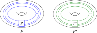
Figure 12. (color online) Patterns $P$ and $P^{\ast}$.

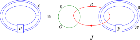
Figure 13. (color online) $X_{P(U)}(0)\cong X_{J}$

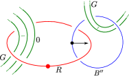
Figure 14. (color online) Slide to vanish the linking number of $G$ and $B^{\prime\prime}$

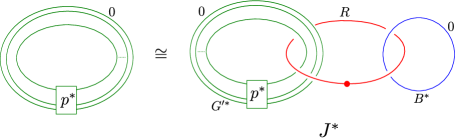
Figure 15. (color online) $X_{P^{\ast}(U)}(0)\cong X_{J^{\ast}}$

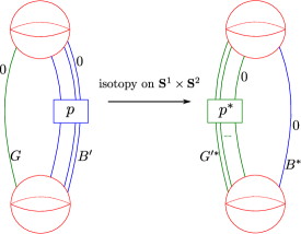
Figure 16. (color online) $X_{J}\cong X_{J^{\ast}}$

Remark 4.5.

We see that Figure 16 gives an alternative proof of Theorem 3.6.

Remark 4.6.

For a pattern $P\colon\mathbf{S}^{1}\rightarrow V$, denote the pattern obtained by twisting $n$ times along a meridian of $V$ by $\tau_{n}(P)$. By utilizing the technique in Figure 16, we can prove that $X_{P(U)}(n)\cong X_{\tau_{n}(P^{\ast})(U)}(n)$ for any $n\in\mathbf{Z}$ (see Figure 17 and see also [14, Theorem 3.6]). Moreover, we can prove that $X_{\tau_{m}(P)(U)}(m+n)\cong X_{\tau_{n}(P^{\ast})(U)}(m+n)$ (see Figure 18).

Baker and Motegi [5, Theorem 2.5] constructed pairs of knots $K_{m}$ and $k_{n}$ which satisfy $M_{K_{m}}(m+n)\cong M_{k_{n}}(m+n)$ for any $m,n\in\mathbf{Z}$. We remark that the pair $\{\tau_{m}(P)(U),\tau_{n}(P^{\ast})(U)\}$ is essentially equal to the pair $\{K_{m},k_{n}\}$.

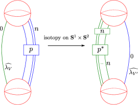
Figure 17. (color online) The left blue curve with framing $n$ is $P\subset V$ and the right green curve with framing $n$ is $\tau_{n}(P^{\ast})\subset V^{\prime}$. We see that $P(U)$ and $\tau_{n}(P^{\ast})(U)$ have the diffeomorphic $n$-trace. The box with the label $n$ means the $n$ full-twists.

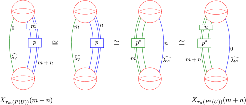
Figure 18. (color online) $X_{\tau_{m}(P)(U)}(m+n)\cong X_{\tau_{n}(P^{\ast})(U)}(m+n)$

4.2. Oriented RGB-diagram

Recall that dualizable patterns are oriented. We can also consider orientations of RGB-diagrams as follows. An RGB-diagram $L=R\cup G\cup B$ is oriented if $G$ and $B$ are oriented so that they are homologous in $\mathbf{S}^{3}\setminus R$. From an oriented RGB-diagram $L$, we can also construct two knots $K_{B}$ and $K_{G}$ as in Section 4.1. Then, we can give orientations of $K_{B}$ and $K_{G}$ by the orientations of $B$ and $G$, respectively.

Let $P$ be a dualizable pattern. In order to construct an oriented RGB-diagram $L=R\cup G\cup B$ from $P$, recall the proof of Lemma 4.4. Firstly, we construct a Kirby diagram $J=R\cup G\cup B^{\prime}$ from $P$ (see Figure 13). Then, we can orient $G$ and $B^{\prime}$ by using the orientations of $\lambda_{V}$ and $P$, respectively. Note that $G$ and $B^{\prime}$ are homologous in $\mathbf{S}^{3}\setminus R$ because of the definition of the orientation of $\lambda_{V}$. Secondly, to construct $L=R\cup G\cup B$ from $J$, we slide $B^{\prime}$ over $R$ finitely many times. After the operation, the linking number of $B^{\prime}$ and $R$ does not change. Hence, $G$ and $B$ are homologous in $\mathbf{S}^{3}\setminus R$, and $L$ is an oriented RGB-diagram.

Recall that the orientations of $B$ and $G$ are given by the orientations of $P$ and $\lambda_{V}$, respectively. Moreover, the orientation of $P^{\ast}$ is given by the orientation of $\lambda_{V}$. Hence, by Lemma 4.4, we see that $K_{B}=P(U)$ and $K_{G}=P^{\ast}(U)$ as oriented knots.

Lemma 4.7 (the oriented version of Lemma 4.4).

For any dualizable pattern $P$, there exists an oriented RGB-diagram $L=R\cup G\cup B$ such that $K_{B}=P(U)$ and $K_{G}=P^{\ast}(U)$ as oriented knots.

4.3. From special annulus presentations to RGB-diagrams

Let $K$ be a knot with a special annulus presentation $(A,b)$. In Section 3.2, we construct a dualizable patterns $P_{\pm}$ such that $P_{\pm}(U)=K$ and $P_{\pm}^{\ast}(U)=A^{\pm 1}(K)$. In this subsection, we draw RGB-diagrams $L_{\pm}=R\cup G_{\pm}\cup B_{\pm}$ such that $K_{B_{\pm}}=P_{\pm}(U)=K$ and $K_{G_{\pm}}=P_{\pm}^{\ast}(U)=A^{\pm 1}(K)$ by utilizing (the proof of) Lemma 4.4. Here, we only consider the case of Figure 8 $(1)$. For three other cases, the similar discussions work.

Let $K$ be a knot with a special annulus presentation $(A,b)$, where $A$ is $-1$ twisted (see the left picture of Figure 19). The dualizable pattern $P=P_{+}\subset\mathbf{S}^{3}\setminus\nu(\beta)$, which satisfies $P(U)=K$ and $P^{\ast}(U)=A^{+1}(K)$, is given as the center picture of Figure 19. Then, the Kirby diagram $J=R\cup G\cup B^{\prime}$ obtained from $P$ as in the proof of Lemma 4.4 is given as the right picture of Figure 19. To obtain the RGB-diagram $L$ given in the proof of Lemma 4.4, firstly slide $B^{\prime}$ over $R$ along the black arrow as in the left picture of Figure 20 and denote the resulting knot by $B^{\prime\prime}$. In the resulting diagram, the linking number of $G$ and $B^{\prime\prime}$ is not zero. So, by sliding $B^{\prime\prime}$ over $R$ along the dotted black arrow as in the center picture of Figure 20, we delete the linking number. Then the resulting diagram is an RGB-diagram $L=R\cup G\cup B$ (see the right picture of Figure 20). This is the desired RGB-diagram $L_{+}=R\cup G_{+}\cup B_{+}$. As a consequence, we obtain Theorem 4.8 below.

Theorem 4.8.

Let $K$ be a knot with a special annulus presentation $(A,b)$. Then, there are dualizable patterns $P_{\pm}$ and RGB-diagrams $L_{\pm}=R\cup G_{\pm}\cup B_{\pm}$ such that $K=P_{\pm}(U)=K_{B_{\pm}}$ and $A^{\pm}(K)=P_{\pm}(U)=K_{G_{\pm}}$. In particular, such $P_{\pm}$ and $L_{\pm}=R\cup G_{\pm}\cup B_{\pm}$ are given as in Figure 21.

By the discussions in Sections 3.3 and 4.2, we obtain the oriented version of Theorem 4.8 as follows.

Theorem 4.9 (the oriented version of Theorem 4.8).

Let $K$ be an oriented knot with a special annulus presentation $(A,b)$. Give $A^{\pm 1}(K)$ the orientation induced by $K$. Then, there are dualizable patterns $P_{\pm}$ and oriented RGB-diagrams $L_{\pm}=R\cup G_{\pm}\cup B_{\pm}$ such that $K=P_{\pm}(U)=K_{B_{\pm}}$ and $A^{\pm}(K)=-P_{\pm}(U)=-K_{G_{\pm}}$. In particular, such $P_{\pm}$ and $L_{\pm}=R\cup G_{\pm}\cup B_{\pm}$ are given as in Figure 21, where the orientations of $P_{\pm}$ and $B_{\pm}$ are induced by $K$ and the orientations of $P_{\pm}^{\ast}$ and $G_{\pm}$ are induced by a meridian of $\beta$ (or $R$) which is homologous to $K$ in $\mathbf{S}^{3}\setminus\beta$.

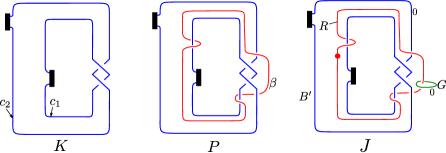
Figure 19. (color online) A knot $K$ with a special annulus presentation (left), a dualizable pattern $P\subset\mathbf{S}^{3}\setminus\nu(\beta)$ satisfying $P(U)=K$ and $P^{\ast}(U)=A^{+1}(K)$ (center) and the Kirby diagram $J$ corresponding to $P$ (right).

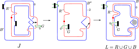
Figure 20. (color online) From $J$ to the RGB-diagram $L$. In the gray area in the right picture, the band (the green component $G$) may appear.

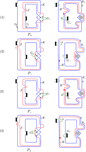
Figure 21. (color online) The left blue curves represent knots $K$ which have special annulus presentations. The patterns $P_{\pm}$ are given by $K$ in $\mathbf{S}^{3}\setminus\nu(\beta)=V$, where the parameters of $V\cong\mathbf{S}^{1}\times D^{2}$ are given so that $P_{\pm}(U)=K$. The right pictures are $L_{\pm}=R\cup G_{\pm}\cup B_{\pm}$. The RGB-diagrams $L_{\pm}$ are obtained from the left pictures by (i) replacing $\beta$ with dotted circles $R$, (ii) regarding $K$ and the green curves $G_{\pm}$ as $0$-framed $2$-handles, (iii) sliding $K$ over $R$ along the black arrows and (iv) sliding $K$ over $R$ along the dotted black arrows. In the gray areas in the right pictures, the band (the green component $G_{\pm}$) may appear.

Remark 4.10.

We remark that there are a dualizable pattern and an RGB-diagram which do not arising from any special annulus presentation. In fact, the four-ball genera $g_{4}$ of knots with annulus presentations are less than $2$. On the other hand, Piccirillo [16, Example 3.4] gave an RGB-diagram whose $K_{G}$ has $g_{4}(K_{G})=2$. Moreover, by Proposition 4.3, we can construct a dualzable pattern $P$ which satisfies $g_{4}(P^{\ast}(U))=2$.

Remark 4.11.

Let $K$ be an unknotting number one knot. It is know that such a knot $K$ has a special annulus presentation (see [1, Lemma 2.2]). Then, by Theorem 4.8, we obtain RGB-diagrams $L_{\pm}=R\cup G_{\pm}\cup B_{\pm}$ from the special annulus presentation. On the other hand, Piccirillo [17] constructed an RGB-diagram from an unknotting number one knot. We see that the RGB-diagram is equal to $L_{+}$ or $L_{-}$.

Example 4.12.

Consider the special annulus presentation of $6_{3}$ given in Figure 2 (and see also Figure 3). By applying Theorem 4.8 and Figure 21 $(4)$, we obtain an RGB-diagram $L=R\cup G\cup B$ from the the special annulus presentation, which satisfies $K_{G}=A(6_{3})$ and $K_{B}=6_{3}$ (see the bottom right picture in Figure 22).

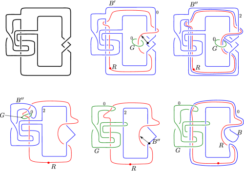
Figure 22. (color online) A special annulus presentation (top left). A Kirby diagram $J$ in Section 4.3 (top center). The bottom left and center pictures are isotopic to the top right picture.

5. Application

In this section, as an application of the discussion in Section 4.3, we introduce a sufficient condition for a knot with a special annulus presentation $(A,b)$ to be either $K=A(K)$ or $K=A^{-1}(K)$.

Theorem 5.1.

Let $K$ be an oriented knot with a special annulus presentation $(A,b)$ with $\partial A=c_{1}\cup c_{2}$. Give $A^{\pm 1}(K)$ the orientation induced by $K$. Let $D_{i}$ be a disk bounded by $c_{i}$ for $i=1,2$. Then if $\operatorname{Int}(D_{i})\cap b=\emptyset$ for some $i$, we obtain either $A(K)=K$ or $A^{-1}(K)=K$ as oriented knots.

Proof.

We only consider the case where $A$ is $-1$ twisted and $D_{1}\cap b=\emptyset$. Then, for the oriented RGB-diagram $L_{+}=R\cup G_{+}\cup B_{+}$ given in Theorem 4.9, there is a disk $D_{R}$ bounded by $R$ such that the intersections $D_{R}\cap G_{+}$ and $D_{R}\cap B_{+}$ consist of exactly one point (see the center of Figure 23, where the points in $D_{R}\cap G_{+}$ and $D_{R}\cap B_{+}$ are drawn by black dots). By the definition of $K_{G_{+}}$ (see Section 4.1), the knot $K_{G_{+}}$ is obtained from $G_{+}$ by sliding $G_{+}$ over $B_{+}$ along the black arrow in the right picture in Figure 23. Similarly, the knot $K_{B_{+}}$ is obtained from $B_{+}$ by sliding $B_{+}$ over $G_{+}$ along the dotted black arrow in the right picture in Figure 23. Hence, we obtain $K_{G_{+}}=K_{B_{+}}$ as unoriented knots. Moreover, since $B_{+}$ and $G_{+}$ are homologous in $\mathbf{S}^{3}\setminus R$, we have $-K_{G_{+}}=K_{B_{+}}$ as oriented knots. By Theorem 4.9, we see that $A^{+1}(K)=-K_{G_{+}}=K_{B_{+}}=K$. ∎

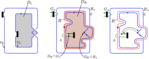
Figure 23. (color online) In the gray area $D_{1}$, the band does not appear (left). The intersections $D_{R}\cap G_{+}$ and $D_{R}\cap B_{+}$ are only one point (center).

Remark 5.2.

It is easy seen that a non-trivial knot satisfying the hypothesis of Theorem 5.1 has unknotting number one. Conversely, a knot of unknotting number one has an annulus presentation which satisfies the hypothesis of Theorem 5.1 by the construction given in [1, Lemma 2.2].

Remark 5.3.

After submitting the first draft of this manuscript to arXiv, in [13, Section 4.2], Manolescu and Piccirillo introduced a result similar to Theorem 5.1.

Example 5.4.

Consider the special annulus presentation of $6_{3}$ given in Figure 2. We see that this annulus presentation satisfies the condition of Theorem 5.1. In [3, Section 2], Abe and the author proved that $6_{3}\neq A(6_{3})$. Hence, by Theorem 5.1, we have $A^{-1}(6_{3})=6_{3}$. We can prove this fact directly (see Figure 24).

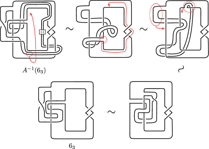
Figure 24. (color online) Direct proof for $A^{-1}(6_{3})=6_{3}$. Note that $6_{3}$ is invertible. The bottom left picture is obtained from the bottom right picture by flipping the annulus $A$.

Acknowledgements. This work was supported by JSPS KAKENHI Grant numbers JP18K13416 and JP22K13923.

References

- [1] T. Abe, I. Jong, Y. Omae, and M. Takeuchi, Annulus twist and diffeomorphic 4-manifolds, Math. Proc. Cambridge Philos. Soc. 155 (2013), no. 2, 219–235. MR 3091516
- [2] T. Abe, I. D. Jong, J. Luecke, and J. Osoinach, Infinitely many knots admitting the same integer surgery and a four-dimensional extension, Int. Math. Res. Not. IMRN (2015), no. 22, 11667–11693. MR 3456699
- [3] T. Abe and K. Tagami, Fibered knots with the same 0-surgery and the slice-ribbon conjecture, Math. Res. Lett. 23 (2016), no. 2, 303–323. MR 3512887
- [4] T. Abe and M. Tange, A construction of slice knots via annulus twists, Michigan Math. J. 65 (2016), no. 3, 573–597. MR 3542767
- [5] K. Baker and K. Motegi, Noncharacterizing slopes for hyperbolic knots, Algebr. Geom. Topol. 18 (2018), no. 3, 1461–1480. MR 3784010
- [6] L. N. Carvalho and U. Oertel, A classification of automorphisms of compact 3-manifolds, arXiv:math/0510610v1.
- [7] R. H. Fox, Some problems in knot theory, Topology of 3-manifolds and related topics (Proc. The Univ. of Georgia Institute, 1961), Prentice-Hall, Englewood Cliffs, N.J., 1962, pp. 168–176. MR 0140100
- [8] D. Gabai, Foliations and the topology of -manifolds. III, J. Differential Geom. 26 (1987), no. 3, 479–536. MR 910018
- [9] R. E. Gompf and K. Miyazaki, Some well-disguised ribbon knots, Topology Appl. 64 (1995), no. 2, 117–131. MR 1340864
- [10] C. McA. Gordon and J. Luecke, Knots are determined by their complements, J. Amer. Math. Soc. 2 (1989), no. 2, 371–415. MR 965210
- [11] J. Johnson, Notes on Heegaard splittings, preprint, 2006.
- [12] R. Kirby., Problems in low-dimensional topology, AMS/IP Stud. Adv. Math. 2(2), Geometric topology(Athens, GA, 1993), 35–473 (Amer. Math. Soc. 1997).
- [13] C. Manolescu and L. Piccirillo, From zero surgeries to candidates for extic definite four-manifolds, arXiv:2102.04391.
- [14] A. N. Miller and L. Piccirillo, Knot traces and concordance, J. Topol. 11 (2018), no. 1, 201–220. MR 3784230
- [15] J. Osoinach, Manifolds obtained by surgery on an infinite number of knots in , Topology 45 (2006), no. 4, 725–733. MR 2236375
- [16] L. Piccirillo, Shake genus and slice genus, Geom. Topol. 23 (2019), no. 5, 2665–2684. MR 4019900
- [17] by same author, The Conway knot is not slice, Ann. of Math. (2) 191 (2020), no. 2, 581–591. MR 4076631
- [18] J. Schultens, The classification of Heegaard splittings for (compact orientable surface), Proc. London Math. Soc. (3) 67 (1993), no. 2, 425–448. MR 1226608
- [19] K. Tagami, Notes on constructions of knots with the same trace, Hiroshima Math. J. 52 (2022), no. 1, 1–15. MR 4399938
- [20] M. Teragaito, A Seifert fibered manifold with infinitely many knot-surgery descriptions, Int. Math. Res. Not. IMRN (2007), no. 9, Art. ID rnm 028, 16. MR 2347296
- [21] F. Waldhausen, Heegaard-Zerlegungen der -Sphäre, Topology 7 (1968), 195–203. MR 0227992
- [22] K. Yasui, Corks, exotic 4-manifolds, and knot concordance, arXiv:1505.0255.