Efficient Joinable Table Discovery in Data Lakes: A High-Dimensional Similarity-Based Approach

Finding joinable tables in data lakes is key procedure in many applications such as data integration, data augmentation, data analysis, and data market. Traditional approaches that find equi-joinable tables are unable to deal with misspellings and different formats, nor do they capture any semantic joins. In this paper, we propose PEXESO, a framework for joinable table discovery in data lakes. We target the case when textual values are embedded as high-dimensional vectors and columns are joined upon similarity predicates on high-dimensional vectors, hence to address the limitations of equi-join approaches and identify more meaningful results. To efficiently find joinable tables with similarity, we propose a block-and-verify method that utilizes pivot-based filtering. A partitioning technique is developed to cope with the case when the data lake is large and cannot fit in main memory. An experimental evaluation on real datasets shows that our solution identifies substantially more tables than equi-joins and outperforms other similarity-based options, and the join results are useful in data enrichment for machine learning tasks. The experiments also demonstrate the efficiency of the proposed method.

I Introduction

Join is a fundamental and essential operation that connects two or more tables. It is also a significant technique applied to relational database management systems and business intelligence tools for data analysis. The benefits of joining tables are not only in the database fields (e.g., data integration) but also in the machine learning (ML) fields such as feature augmentation and data enrichment [20, 5].

With the trends of open data movements by governments and the dissemination of data lake solutions in industries, we are provided with more opportunities to obtain a huge number of tables from data lakes (e.g., WDC Web Table Corpus [28]) and make use of them to enrich our local data. As such, a local table can be regarded as a query, and our request is to look for joinable tables in the data lake. Many researchers studied the problem of data discovery in data lakes. Unfortunately, existing works on finding joinable tables [37, 39] only focused on evaluating the joinability between columns by taking the overlap number of equi-joined records. One example is joining the “Race” column in Table I(a) with the “Col_1” column in Table I(b). “White” and “Black” yield equi-join results as strings exactly match in the two columns. However, the tables in data lakes usually do not have an explicitly specified schema and heterogeneous tables may differ in representations or terminologies, e.g., “American Indian/Alaska Native” v.s. “Mainland Indigenous”, and “Hawaiian/Guamanian/Samoan” v.s. “Pacific Islander”. In these cases, equi-joins fail to capture the semantics. They either produce few join results if we use an inner-join, or cause sparsity if we use a left-join. This may not improve the effectiveness for ML tasks and sometimes even degrades the quality due to overfitting. On the other hand, despite a few recent studies on non-equi-joins, e.g., by string transformation [38] or statistical correlation [13], they only deal with the case of joining two given tables; it is unknown how to find joinable tables in a data lake, and it is prohibitive to try joining every table in the data lake with the query table. Other recent advances, such as [7] and [10], can help users search for desired attributes in a data lake semantically, yet they do not consider if the identified columns are really joinable.

A deeper view on the semantic level, such as utilizing word embeddings, enables us to identify text with the same or similar meanings, hence to tackle the data heterogenity. We can solve the aforementioned drawbacks of equi-joins and cope with the joinable table search problem by representing each record of a column (in contrast to [10] which uses word embeddings on column names) as a high-dimensional vector, and a column is thus represented as a multiset of high-dimensional vectors. Then, we can leverage the similarity between vectors to evaluate the joinability between columns.

TABLE I: An example of semantically joinable tables.

(a) Population.

Race	Population	Median Age
White	234,370,202	42.0
Black	40,610,815	32.7
American Indian/Alaska Native	2,632,102	31.7
Hawaiian/Guamanian/Samoan	570,116	29.7

(b) Median household income (US$).

Col_1	Col_2
White	65,902
Black	41,511
Mainland Indigenous	44,772
Pacific Islander	61,911

In this paper, we study the problem of joinable table discovery in data lakes and explore in the direction of embedding records as high-dimensional vectors and joining upon similarity predicates. To the best of our knowledge, this is the first work targeting high-dimensional similarity on record embeddings for joinable table discovery. Some recent studies deal with the problem of joining tables for feature augmentation [20, 5], where a few candidate tables are assumed to be ready for join. They focused on efficient feature selection over these candidate tables; however, the assumption of the availability of candidate tables does not always hold, and our proposed solution can be used to feed them with such candidates.

The problem of finding joinable tables with high-dimensional similarity has two challenges. First, the similarity computation for high-dimensional data is expensive. For example, GloVe [12] transforms a word to a 50- to 300-dimensional vector. It is prohibitive to exhaustively compute the similarities between all pairs of records. Second, the number of tables in a data lake is large. It is time-consuming to check whether the tables are joinable or not one by one. Existing research on high-dimensional similarity focused on searching an object or joining two datasets efficiently (see [26] for a survey), but none of them were designed for searching for joinable table with similarity predicates.

Seeing the above challenges, we propose a framework called PEXESO to efficiently find joinable tables with high-dimensional similarity. PEXESO mainly deals with textual columns and support any similarity function in a metric space. The joinability of a table is measured by the number of matching records in the query column, which are defined using a distance function and a threshold. PEXESO adopts a block-and-verify strategy to reduce the similarity computation between records. We employ pivot-based filtering to select a set of pivot vectors and compute the distances to these pivots to prune vectors by the triangle inequality. Then hierarchical grids, which divide the pivot space into cells, are utilized to block vectors and find candidates. Finally, we verify the candidates to count the number of matching records with the help of an inverted index. Our search algorithm finds exact answers to the joinable table search problem with similarity predicates. We analyze its complexity and cost. For the case of a large-scale data lake that cannot be loaded in main memory, we resort to data partitioning and load each part with a single PEXESO. We develop a clustering method that partitions the dataset by column distributions.

We conduct experiments on real datasets and evaluate on ML tasks to show the effectiveness of our similarity-based approach of joinable table discovery as well as its usefulness in enriching data for ML. PEXESO achieves 0.21 – 0.28 higher recall than the equi-join approach and outperforms the approaches using other similarity options such as Jaccard and fuzzy-join [32] in both precision and recall. By using PEXESO for data enrichment, the performance of the ML tasks is improved by 1.9% higher micro-F1 score and 10% lower mean squared error. As for efficiency, PEXESO outperforms exact baselines by up to 76 times speedup. Its processing speed is competitive with the approximate solution of product quantization [16] (which has very low precision and recall in finding joinable tables) and even better in some cases.

Our contributions are summarized as follows. (1) We propose PEXESO, a framework for joinable search discovery in data lakes. Our solution targets textual values embedded as high-dimensional vectors in a metric space and columns are joined upon similarity predicates. (2) To efficiently find joinable tables upon similarity predicates, we design a block-and-verify solution based on hierarchical grids and an inverted index. Our algorithm employs pivot-based filtering to reduce similarity computation. (3) We propose data partitioning for the out-of-core case. A clustering method is developed to partition the dataset. (4) We conduct experiments on real datasets to demonstrate the effectiveness and the efficiency of PEXESO in finding joinable tables and its usefulness in building ML models.

A caveat is that we do not target a specific representation learning approach but efficiency optimization for the case when records are embedded in a metric space. Our design decouples effectiveness and efficiency optimizations. Any representation learning model can be used in our framework to transform the original data to vectors, as long as the output is in a metric space. The embedding approaches and the similarity we use in the experiments, according to the taxonomy in [24], belong to the category of character-level pre-trained embedding, heuristic-based summation, and fixed distance comparison. As such, our solution renders the entire workflow unsupervised without any labelling work. We discover that this has already achieved better results than equi-join and non-semantic similarity approaches. We believe that more sophisticated models outlined in the design space [24] may perform better, but this is specific to the task and may require labelled examples for training.

The rest of the paper is organized as follows. Section II overviews the PEXESO framework and defines the joinable table search problem. Section III presents our indexing and search algorithm. Section IV introduces data partitioning for large-scale data lakes. Section V discusses threshold specification in PEXESO. Experimental results are reported and analyzed in Section VI. Section VII reviews related work. Section VIII concludes the paper.

II Joinable Table Discovery Framework

II-A System Overview

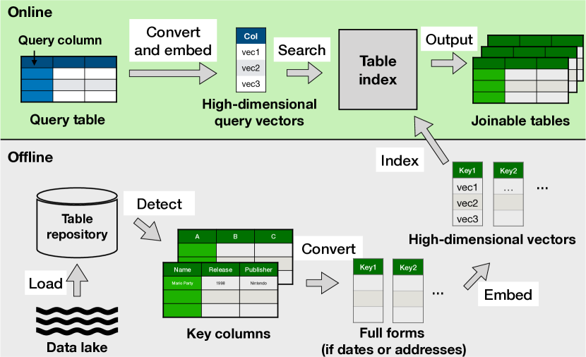
Figure 1: Joinable table discovery framework.

Fig. 1 shows an overview of our PEXESO framework, which consists of two components:

• The offline component loads raw data (e.g., in CSV format) from the data lake to a table repository and extracts the columns that are expected to be join keys. For example, the WDC Web Table Corpus [28] contains key column information. We may also use the SATO method [35] to detect data types in tables and choose the columns whose types (e.g., names) can serve as a join key. For each string (including date) column, we transform the records (i.e., the string values rather than the column name) to high-dimensional vectors by a pre-trained model, e.g., fastText [9], which carries semantic information and handles misspelling by making use of character-level information. In this sense, the pre-trained model can be regarded as a plug-in in our framework, and thus any representation learning method can be used here. For out-of-vocabulary words, the similarity can still be captured if we use subword embeddings. Another option is using the embedding of the most literally similar word or averaging the embeddings of the nearby context words. To handle date and address columns, in which abbreviations often exist, we first convert abbreviations to their full forms (e.g., “Mar” to “March” and “St” to “Street”) and then apply the pre-trained model. When applying our method to domain-specific tables, we may leverage existing abbreviation dictionaries or knowledge bases for the domain, or learn a dictionary of abbreviation rules [30]. The high-dimensional vectors are indexed for efficient lookup.

• The online component takes as input the user’s query table, which contains a query column for join. There are several options to determine the query column: (1) the user specifies the query column, (2) we choose the string column with the most distinct values, and (3) we iterate through all the columns and regard each as a query column. Without loss of generality, we assume the first option, in line with [37], and our techniques can be easily extended to support the other two options. We focus on the case of string columns as this is the most common data type in many data lakes (e.g., 65% columns are strings in the WDC Web Table Corpus); for other data types, equi-join is used and this case has been addressed by Zhu et al. [37]. The values in the query column are transformed to high-dimensional vectors using the same pre-trained model as in the offline component. Dates and addresses are also handled in the same way. Then we employ similarity predicates to define joinability and search for joinable tables in the repository. To present the results, we show the user a set of joinable tables along with the mapping between the records in the query column and the target column, since the user might not be familiar with our join predicates.

II-B Similarity-Based Joinability

Next we present a formal definition of the joinable table search problem. Table II summarizes the notations frequently used in this paper.

TABLE II: Frequently used notations.

Symbol	Description
$Q,S$	a query column, a target column in the repository
$R$	a collection of target columns (i.e., the repository)
$R_{V}$	a collection of all the vectors in $R$’s columns
$q,x$	a query vector in $Q$, a target vector in the repository
$d(\cdot,\cdot)$	a distance function
$\tau,T$	a distance threshold, a column joinability threshold
$M_{\tau}^{d}(a,b)$	an indicator that indicates if $a$ matches $b$
$jn_{\tau}^{d}(Q,S)$	the joinability of $S$ to $Q$
$p,P$	a pivot vector, a set of pivot vectors
$SQR(q^{\prime},\tau)$	a square query region
$RQR(q^{\prime},p,\tau)$	a rectangle query region
$HG_{Q},HG_{R_{V}}$	hierarchical grids for the mapped vectors of $Q$ and $R_{V}$
$m$	the number of levels in a hierarchical grid
$I$	an inverted index

To match records at the semantic level, we consider vectors in a metric space and define the notion of vector matching under a similarity condition.

Definition 1 (Vector Matching).

Given two vectors $v_{1}$ and $v_{2}$ in a metric space, a distance function $d$, and a threshold $\tau$, we say $v_{1}$ matches $v_{2}$, or vice versa, if and only if $d(v_{1},v_{2})\leq\tau$.

We use notation $M_{\tau}^{d}(v_{1},v_{2})$ to denote if $v_{1}$ matches $v_{2}$; i.e., $M_{\tau}^{d}(v_{1},v_{2})=1$, iff. $d(v_{1},v_{2})\leq\tau$, or 0, otherwise.

Given a query column $Q$ and a target column $S$, we use the number of matching vectors to define the joinability upon distance $d$ and threshold $\tau$, which counts the number of vectors in $Q$ having at least one matching vector in $S$, normalized by by the size of $Q$, i.e.,

$$jn_{\tau}^{d}(Q,S)=\frac{|Q_{M}|}{|Q|},$$

$$Q_{M}=\{\,q\mid q\in Q\wedge\exists x\in S\text{\, s.t.\, }M_{\tau}^{d}(q,x)=1\,\}.$$

Note the above joinability is not symmetric, i.e., we count matching vectors in $Q$ rather than $S$. We say the columns $Q$ and $S$ are joinable, if and only if the joinability $jn_{\tau}^{d}(Q,S)$ is larger than or equal to a threshold $T$. We also say that the tables containing these two columns are joinable. Next we define the joinable column (table) search problem.

Definition 2 (Joinable Column (Table) Search).

Given a collection of columns $R$, a query column $Q$, a distance function $d$, a distance threshold $\tau$, and a joinability threshold $T$, the joinable column (table) search problem is to find all the columns in $R$ that are joinable to the query column $Q$, i.e., $\{\,S\mid S\in R\wedge jn_{\tau}^{d}(Q,S)\geq T\,\}$.

Duplicate values may exist in the query column. We regard them as independent records in the join predicate, because even if two records may share the same value in the query column, they may pertain to different entities.

III Indexing and Search Algorithm

A naive method for the joinable table search problem is for each vector in $Q$, computing the distance to all the vectors in all the columns of $R$ and counting the number of matching vectors to determine if a column is joinable. The distance is computed $|Q|\cdot\sum_{S\in R}|S|$ times. Hence it is prohibitive when the number of vectors is large. To solve this problem efficiently, our key idea is to reduce the distance computation. We propose an algorithm that employs a block-and-verify strategy: the vectors of the query column and the target columns are blocked in hierarchical grids, and then candidates are produced by joining the cells in the hierarchical grids. We verify the candidates (i.e., to compute the exact distance between vectors) with the help of an inverted index while computing the joinabilities of the target columns. Our solution utilizes pivot-based filtering, which yields an exact answer of the problem. We do not choose approximate approaches to high-dimensional similarity query processing because they do not bear non-probability guarantee on the number of matching vectors and result in very low precision and recall (see Section VI-B). We begin with preliminaries on pivot-based filtering.

III-A Preliminaries on Pivot-based Filtering

The pivot-based filtering [4] uses pre-computed distances to prune vectors on the basis of the triangle inequality. The distance from each vector to a set of pivot vectors $P$ is pre-computed and stored. Then mismatched vectors can be pruned using the following lemma.

Lemma 1 (Pivot Filtering).

Given two vectors $q$ and $x$, a set $P$ of pivot vectors, a distance function $d$, and a threshold $\tau$, if $q$ matches $x$, then $d(q,p)-\tau\leq d(x,p)\leq d(q,p)+\tau$.

Proof.

We prove by contradiction. Assume that there exists an vector $x$ matches with $q$, i.e., $d(q,x)\leq\tau$, but for a pivot $p$, it holds $d(x,p)\notin[d(q,p)-\tau,d(q,p)+\tau]$, i.e., $|d(x,p)-d(q,p)|>\tau$. By the triangle inequality, $d(q,x)\geq|d(x,p)-d(q,p)|>\tau$, and this contradicts the assumption. ∎

Matching vectors can be identified using the following lemma.

Lemma 2 (Pivot Matching).

Given two vectors $q$ and $x$, a set $P$ of pivot vectors, a distance function $d$, and a threshold $\tau$, if there exists a pivot $p\in P$ such that $d(x,p)+d(q,p)\leq\tau$, then $q$ matches $x$.

Proof.

For a pivot $p$, the triangle inequality holds: $d(q,p)+d(x,p)\geq d(q,x)$. If $d(x,p)\leq\tau-d(q,p)$, then $d(x,p)+d(q,p)\leq\tau$. Therefore, $d(q,x)<\tau$ and $x$ is matched with $q$. ∎

To utilize the above lemmata, pivot mapping was introduced [4]. Given a set of pivots $P=\{p_{1},p_{2},...,p_{n}\}$, the pivot mapping for a vector $x$ involves computing the distance between $x$ and all the pivots in $P$, and assembling these values in a mapped vector $x^{\prime}$. Specifically, $x$ is mapped to the pivot space of $P$ as $x^{\prime}=[d(p_{1},x),d(p_{2},x),...,d(p_{n},x)]$. The pivot size should be smaller than the dimensionality of the original metric space, so that the dimensionality can be reduced through range query processing in the pivot space to avoid the curse of dimensionality. Next we use an example to illustrate how to reduce distance computation by pivot mapping.

Fig. 2 shows an example in a 2-$d$ metric space. A query column $Q$ has two vectors: $Q=\{\,q_{1},q_{2}\,\}$. There are four target columns in the table repository, each of them having two vectors: $S_{1}:\{\,x_{1},x_{2}\,\}$, $S_{2}:\{\,x_{3},x_{4}\,\}$, $S_{3}:\{\,x_{5},x_{6}\,\}$, $S_{4}:\{\,x_{7},x_{8}\,\}$. These vectors are represented as points in a 2-$d$ metric space. Suppose $x_{1}$ and $x_{8}$ are selected as pivots and all the vectors are mapped to a 2-$d$ pivot space. In the pivot space, for each query vector $q$ and the distance threshold $\tau$, a square query region $SQR(q^{\prime},\tau)$ is created, with $q$’s mapped vector $q^{\prime}$ as the center and $2\tau$ as edge length. By Lemma 1, all the vectors outside the square query region $SQR(q^{\prime},\tau)$ can be safely pruned from the result of the range search in the original metric space; i.e., none of them matches $q$. Therefore, only the vectors located in $SQR(q^{\prime},\tau)$ need to be computed if they match $q$ via distance computation. In Fig. 2, only $x_{2},x_{4},x_{6},x_{7}$, whose mapped vectors are located in the square query region $SQR(q_{1}^{\prime},\tau)$ (in red), need distance computation against $q_{1}$.

To use Lemma 2 and find matching vectors, for each query $q$ and each pivot $p_{i}\in P$, a rectangle query region $RQR(q^{\prime},p_{i},\tau)$ is created. It starts from the original point $(0,0)$; the edge length in the $i$-th dimension is $\tau-d(q,p)$, and the other edges have an infinite length. An exception is that the rectangle query region is not created for pivot $p_{i}$ when $\tau-d(q,p)$ is negative. By Lemma 2, all the vectors in $RQR(q^{\prime},p,\tau)$ match query $q$. In Fig. 2, $q_{1}^{\prime}$ has no rectangle query region for pivot $x_{1}$ or $x_{8}$ (due to negative edge length), and $q_{2}^{\prime}$ has a rectangle query region $RQR(q_{2}^{\prime},x_{1},\tau)$ (in green) for pivot $x_{1}$, denoted as. Because $x_{3}^{\prime}$ is located in this region, $x_{3}$ is guaranteed to match $q_{2}$ and thus there is no need to compute distance for them.

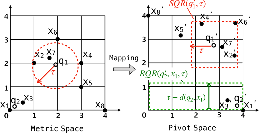
Figure 2: Example of pivot mapping with pivots $x_{1}$ and $x_{8}$, a square query region of pivot filtering for $q_{1}$ (red), and a rectangle query region of pivot matching for $q_{2}$ (green).

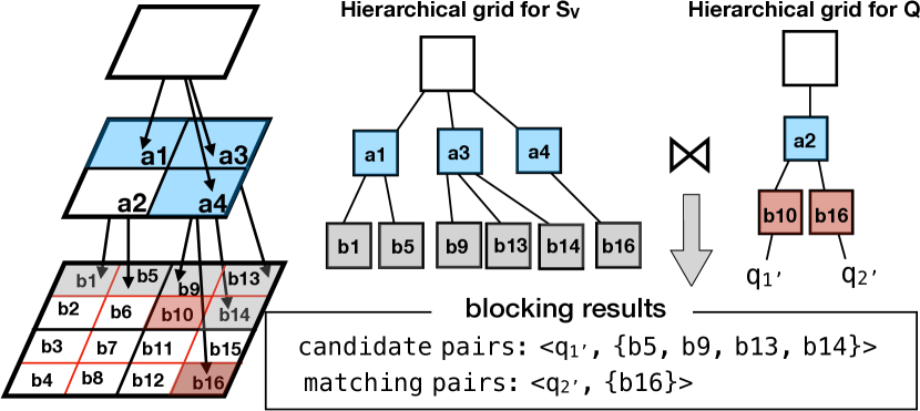
Figure 3: Hierarchical grids for target vectors and query vectors, and the blocking results of matching pairs and candidate pairs.

III-B Blocking with Hierarchical Grids

Using the above techniques, we still need to check target vectors (i.e., the vectors in the columns of the table repository) against the query region of each query vector. To remedy this, we group vectors and employ pivot-based filtering to prune in a group-group manner, so the comparison between vectors and query regions can be significantly reduced.

To achieve this, we propose to group similar mapped vectors. The pivot space is equally partitioned into small (hyper-) cells, and we manage the cells in a hierarchical grid with multiple levels of different partitioning granularity. We consider a hierarchical grid of $m$ levels (except the root) and divide the pivot space into $2^{|P|\cdot i}$ partitions, where $|P|$ is the dimensionality of the pivot space and $i\in[1\,\ldotp\ldotp m]$ is the level number. Fig. 3 shows an example of a 2-level hierarchical grid for the mapped vectors of $R_{V}$ in Fig. 2. For the 2-$d$ pivot space, we have two levels with $2^{2\times 1}=4$ cells and $2^{2\times 2}=16$ cells. Note that to save memory, the hierarchical grid only indexes the cells that have at least one vector. As such, in Fig. 3, the leaf level has cells $b_{1}$, $b_{5}$, $b_{9}$, $b_{13}$, $b_{14}$ and $b_{16}$, and the intermediate level has cells $a_{1}$, $a_{3}$ and $a_{4}$.

Based on the above grouping strategy, Lemma 1 yields the following filtering principle.

Lemma 3 (Vector-Cell Filtering).

Given a cell $c$ and a mapped query vector $q^{\prime}$ in the pivot space, if $c\cap SQR(q^{\prime},\tau)=\emptyset$, then for any mapped vector $x^{\prime}\in c$, its original vector $x$ does not match the query vector $q$.

Proof.

$c\cap SQR(q^{\prime},\tau)=\emptyset$ means none of the vectors in $c$ is located in $SQR(q^{\prime},\tau)$. For each mapped vector $x^{\prime}\in c$, its original vector $x$ satisfies that $d(x,p)\notin[d(q,p)-\tau,d(q,p)+\tau],\forall p\in P$. Hence by Lemma 1, $x$ does not match $q$. ∎

We can also group the mapped query vectors into cells and compute a square query region for each cell $c_{q}$ as $SQR(c_{q}.center,\tau+\frac{c_{q}.length}{2})$, where $c_{q}.center$ is the center of the cell and $c_{q}.length$ is the edge length of the cell. To differentiate the two types of cells, the cells in the hierarchical grid for $R_{V}$ are target cells, and those in the hierarchical grid for $Q$ are query cells. Then, by Lemma 1 we have

Lemma 4 (Cell-Cell Filtering).

Given a target cell $c$ and a query cell $c_{q}$ in the pivot space, if $c\cap SQR(c_{q}.center,\tau+\frac{c_{q}.length}{2})=\emptyset$, then for any mapped vector $x^{\prime}\in c$ and any query vector $q^{\prime}\in c_{q}$, their original vectors do not match.

Proof.

For any vector outside $SQR(c_{q}.center,\tau+\frac{c_{q}.length}{2})$, its original vector $x$ satisfies that $d(x,c_{q}.center)>\tau+\frac{c_{q}.length}{2}$, and for each $q^{\prime}\in c_{q}$, its original vector satisfies that $d(q,c_{q}.center)<\frac{c_{q}.length}{2}$. Therefore, for any original vector $x$ and query vector $q$, $d(x,q)>\tau$. ∎

Similar to the above strategy, we also extend Lemma 2 to vector-cell matching and cell-cell matching:

Lemma 5 (Vector-Cell Matching).

Given a target cell $c$ and a mapped query vector $q^{\prime}$ in the pivot space, if there exists a pivot $p\in P$ such that $c\cap RQR(q^{\prime},p,\tau)=c$, then for any vector $x^{\prime}\in c$, the original vector $x$ matches the query vector $q$.

Proof.

For pivot $p\in P$, $c\cap RQR(q^{\prime},p,\tau)=c$ means all the vectors in $c$ are inside the region $RQR(q^{\prime},p,\tau)$, and for each vector $x^{\prime}\in c$, its original vector $x$ satisfies that $d(x,p)\leq\tau-d(q,p)$. By Lemma 2, $x$ matches $q$. ∎

For each pivot $p\in P$, we define the minimum rectangle query region as the intersection of all the $RQR(\cdot,\cdot,\cdot)$ of all the mapped query vectors in $c_{q}$, and denote the minimum rectangle query region as $\min(RQR(q^{\prime},p,\tau)),q^{\prime}\in c_{q}$. If any mapped query vector $q^{\prime}\in c_{q}$ does not have a rectangle query region with a pivot $p$ due to negative edge length, then we define $\min(RQR(q^{\prime},p,\tau))$ as an empty region.

Lemma 6 (Cell-Cell Matching).

Given a target cell $c$ and a query cell $c_{q}$ in the pivot space, if there exists a pivot $p\in P$ such that $c\cap\min(RQR(q^{\prime},p,\tau))=c$, then for any mapped vector $x^{\prime}\in c$ and any query vector $q^{\prime}\in c_{q}$, their original vectors match.

Proof.

For a pivot $p\in P$, if $\min(RQR(q^{\prime},p,\tau))$ exists, then all the query vectors has rectangle query regions for $p$. Therefore, if $c\cap\min(RQR(q^{\prime},p,\tau))=c$, $c$ must be covered by all of these rectangle query regions. By Lemma 2, for any mapped vector $x^{\prime}\in c$ and any query vector $q^{\prime}\in c_{q}$, their original vectors satisfy $d(x,q)\leq\tau$. ∎

We index the mapped vectors of $Q$ and $R_{V}$ in two hierarchical grids $HG_{Q}$ and $HG_{R_{V}}$. They slightly differ in structure: $HG_{Q}$ associates the mapped vectors of $Q$ in its leaf cells, but $HG_{R_{V}}$ does not (see Fig. 3). The reason for such design is because the blocking phase aims to find pairs in the form of $\langle mapped~{}query~{}vector,leaf~{}cells\rangle$. There are two kinds of pairs found: matching and candidate pairs. Matching pairs are vector-cell pairs that satisfy Lemma 5. Candidate pairs are pairs that cannot be filtered by Lemma 3 or Lemma 4. In Fig. 3, the blocking result is $\langle q_{2}^{\prime},\{\,b16\,\}\rangle$ for matching pairs and $\langle q_{1}^{\prime},\{\,b5,b9,b13,b14\,\}\rangle$ for candidate pairs. We use the form of $\langle mapped~{}query~{}vector,leaf~{}cells\rangle$ because the vectors in different columns of $R$ may share a common leaf cell in $HG_{R_{V}}$. Pairing leaf cells (instead of vectors or columns) with mapped query vectors exploits such share and yields efficient verification, as will be introduced later.

Input : parent cell $C_{Q}$, parent cell $C_{R}$, matching pair set $mPair$, candidate pair set $cPair$

1 foreach child $c_{Q}\in C_{Q}$ do

2       foreach child cell $c_{R}\in C_{R}$ do

3             if $c_{Q}$ and $c_{R}$ are leaf cells then

4                   foreach vector $q^{\prime}\in c_{Q}$ do

5                         if $q$ and $c_{R}$ are matched by Lemma 5 then

6                               $mPair\leftarrow mPair\cup\{\,q^{\prime},\{\,c_{R}\,\}\,\}$ ;

7                              

8                        else

9                               if $q^{\prime}$ and $c_{R}$ are not filtered by Lemma 3 then

10                                     $cPair\leftarrow cPair\cup\{\,q^{\prime},\{\,c_{R}\,\}\,\}$ ;

11                                    

12                              

13                        

14                  

15            else

16                   if $c_{Q}$ and $c_{R}$ are matched by Lemma 6 then

17                         $mPair\leftarrow mPair\cup\langle q^{\prime},\{\,c\,\}\rangle$, for each vector $q^{\prime}\in c_{Q}$ and leaf cell $c\in c_{R}$ ;

18                        

19                  else

20                         if $c_{Q}$ and $c_{R}$ are not filtered by Lemma 4 then

21                               $\textsf{Block}(c_{Q},c_{R},mPair,cPair)$;

22                              

23                        

24                  

25            

26      

Algorithm 1 $\textsf{Block}(C_{Q},C_{R},mPair,cPair)$

To retrieve matching and candidate pairs efficiently, $HG_{Q}$ and $HG_{R_{V}}$ are constructed with the same number of levels. We propose an algorithm (Algorithm 1) which follows a block nested loop join style but in a hierarchical way and scans $HG_{Q}$ and $HG_{R_{V}}$ only once. In particular, cells in $HG_{R_{V}}$ are pruned with the same level cells in $HG_{Q}$, and the sub-cells (i.e., children) are expanded at the same time on two hierarchical grids. We use Lemmata 4 and 6 to filter and match non-leaf cells, and use Lemmata 3 and 5 to filter and match leaf cells. Finally, the pairs of query vectors and corresponding leaf cells in $HG_{R_{V}}$ are retrieved as either candidate or matching pairs.

III-C Verifying with an Inverted Index

After obtaining the matching pairs and candidate pairs, for each candidate pair $\langle mapped~{}query~{}vector,leaf~{}cells\rangle$, we compute the distances for the query vector and the target vectors in the leaf cells, and if they match, we increment the joinability count of the column having the target vector. We employ an inverted index in which the leaf cells of $HG_{R_{V}}$ are keys and each key corresponds to a postings list of columns associated with that key (i.e., having at least one vector in that cell).

Fig. 4 shows an example of the inverted index. We can look up the inverted index using the candidate and the matching pairs. We use two global maps to record two numbers: a match map that records the number of matched vectors and an mismatch map that records the number of mismatched vectors for each target column in the table repository. These recorded numbers are used to compute joinability for determining joinable columns.

For each matching pair, we increment the match map for the columns in the postings list. For each candidate pair, we look up the posting lists for the leaf cells in the candidate pair. During the lookup, we access the vectors indexed in the cell and use Lemmata 1 and 2 to filter and match these vectors. If any vector cannot be filtered or matched, we compute the exact distance to the query vector and update the match or mismatch map. Moreoever, we employ a DaaT (document-at-a-time [2]) paradigm for the inverted index lookup, where each column is regarded as a document. So columns in the inverted index are accessed by increasing order of ID. To implement this, we maintain a pointer for each postings list and pop the column with the smallest ID using a priority queue. For the sake of efficiency, we do not materialize a pointer for every cell but only those appear in the candidate set of the query vector. The benefit of the DaaT lookup is that it favors two early termination techniques: (1) whenever the joinability of a column exceeds the threshold $T$ during verification, it is marked as joinable and we can skip processing any vector in this column, and (2) if a column has too many mismatched vectors and the remaining number of candidates are not enough to make the matched vectors exceed $T$, we can early terminate the verification of this column, as stated by the following filtering principle.

Lemma 7.

Given a query column $Q$ and a target column $S$, let $U$ be any subset of $Q$ such that none of the vectors in $U$ match any vector in $S$. If $|Q|-|U|<T$, then $S$ is not a joinable column to $Q$.

Proof.

We prove by contradiction. Assume that $S$ is joinable to $Q$ and $|Q|-|U|<T$. Since there are at most $|Q|-|U|<T$ matching vectors in $Q\backslash U$, there exists at least one vector in $U$ such that the vector matches at least one vector in $S$. This contradicts the definition of $U$. ∎

Fig. 4 shows the verification of matching pair $\langle q_{2}^{\prime},\{\,b16\,\}\rangle$ and candidate pairs $\langle q_{1}^{\prime},\{\,b5,b9,b13,b14\,\}\rangle$. Assume $T=2$. In step 1, for $\langle q_{2}^{\prime},\{\,b16\,\}\rangle$, we update $S_{1}$ and $S_{2}$ in the match map because they belong to the postings list of $b16$. Then we process $\langle q_{1}^{\prime},\{\,b5,b9,b13,b14\,\}\rangle$. In step 2, we check cell $b14$ of column $S_{1}$, denoted by $S_{1}.b14$. Since $S_{1}.b14$ has a vector $x_{2}$ and it matches $q_{1}$, $S_{1}$ in the match map is updated to 2. $S_{1}$ becomes a joinable column as the number of matching vectors reaches $T$. In step 3, by the DaaT lookup, we reach $S_{2}.b9$, which has a vector $x_{4}$. Since it does not match $q_{1}$, $S_{2}$ in the mismatch map is updated to 1. In the same way, $S_{3}$ in the mismatch map is updated to 1 in step 4. After step 4, we do not need to check $S3.b13$ since the mismatch number for $S_{3}$ is 1, and $S_{3}$ can be filtered by Lemma 7. In step 5, we check $S4.b14$ and update the match map. The verification is finished and the result is $S_{1}$. Algorithm 2 gives the pseudocode of the verification.

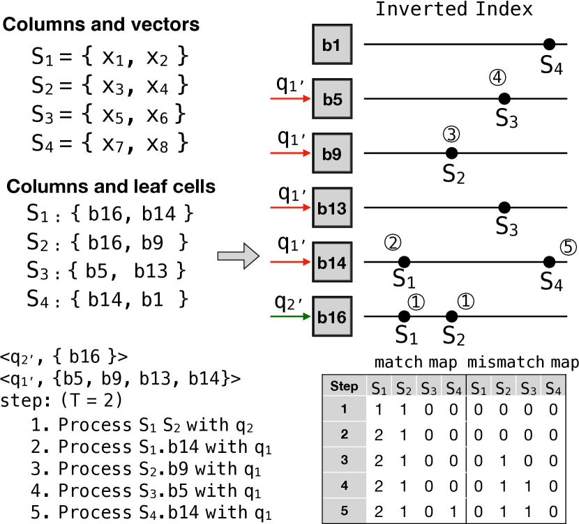
Figure 4: Inverted index for columns and leaf cells.

Input : matching pair set $mPair$, candidate pair set $cPair$, inverted index $I$, thresholds $\tau$ and $T$

1

2foreach $\langle q^{\prime},\{\,c\,\}\rangle\in mPair$ do

3       foreach leaf cell $c\in\{\,c\,\}$ do

4             Update the match map for the columns in $c$;

5            

6      

7

8foreach $\langle q^{\prime},\{\,c\,\}\rangle\in cPair$ do

9       foreach leaf cell $c\in\{\,c\,\}$ do

10             foreach column $S$ having at least one vector in $c$ do

11                   if $S$ can be filtered by Lemma 7 then

12                         continue

13                  else

14                         foreach vector $v^{\prime}\in c$ that belongs to $S$ do

15                               if original vector $v$ of $v^{\prime}$ is filtered by Lemma 1 then

16                                     Update mismatch map for $S$;

17                                    

18                              else if $v$ is matched by Lemma 2 then

19                                     Update match map for $S$;

20                                    

21                              else

22                                     Compute $d(q,v)$ and $M_{\tau}^{d}(q,v)$;

23                                     Update match map or mismatch map for $S$;

24                                    

25                              if $jn_{\tau}^{d}(Q,S)\geq T$ then

26                                     Mark $S$ as a joinable;

27                                     continue

28                              

29                        

30                  

31            

32      

return the columns marked as joinable

Algorithm 2 $\textsf{Verify}(mPair,cPair,I,\tau,T)$

Quick browsing for inverted index. Because we construct $HG_{Q}$ and $HG_{R_{V}}$ with the same level number, the leaf cells between them are also in the same granularity. If a query leaf cell and a target leaf cell refer to the same space region, then we can make sure that they cannot be filtered by Lemma 3 or 4. In this case, the query vectors and the target cell form candidate pairs. Therefore, we can get the leaf cells in $HG_{Q}$ and probe them in the inverted index directly. We call the above process quick browsing. It processes some candidates in advance before running Algorithm 1. Moreover, if quick browsing is issued, we can adjust Algorithm 1 easily for skipping the candidates in the same cell and avoiding redundant computations.

Input : query column $Q$, hierarchical grid $HG_{R_{V}}$, inverted index $I$, thresholds $\tau$ and $T$

Output : Joinable column set $J$

1

2Construct $HG_{Q}$;

3 Look up $I$ by quick browsing with $HG_{Q}.leafCell$ and update match and mismatch maps;

4 matching pair set $mPair\leftarrow\emptyset$, candidate pair set $cPair\leftarrow\emptyset$;

5 $\textsf{Block}(HG_{Q}.root,HG_{R_{V}}.root,mPair,cPair)$;

6 $J\leftarrow\textsf{Verify}(mPair,cPair,I,\tau,T$);

return $J$

Algorithm 3 $\textsf{PEXESO}(Q,HG_{R_{V}},I,\tau,T)$

III-D Pivot Selection

The selection of pivots can significantly affect the performance of pivot filtering. Good pivots can map original vectors and make them scattered in the pivot space, so as to make the query region cover fewer mapped vectors and filter more ones. Previous studies on pivot selection [4, 3, 22] have drawn the conclusion that good pivots are outliers but outliers are not always good pivots. Hence many methods [4, 3, 22] pick outlier vectors as candidates and then select good pivots from them. Here, we adopt the PCA-based method [22] to select high quality pivots in $O(|R_{V}|)$-time.

III-E Search Algorithm and Complexity & Cost Analysis

We assemble the above techniques and present an algorithm (Algorithm 3) for solving the joinable table search problem.

Time complexity. The mapping and construction of the hierarchical grid for $Q$ has a complexity of $O((|P|+m)\cdot|Q|)$. The quick browsing and the block-and-verify method are $O(log|Q|\cdot log|R_{V}|)$. The total time complexity of search is $O((|P|+m)\cdot|Q|+log|Q|\cdot log|R_{V}|)$.

For the construction of PEXESO, we used a PCA-based pivot selection algorithm with a complexity of $O(|R_{V}|)$. Pivot mapping takes $O(|P|\cdot|R_{V}|)$-time. For building the index, it takes $O(m\cdot|R_{V}|)$-time for the hierarchical grid and $O(D)$ for the inverted index, where $D$ is the total number of cells in all the columns. The total time complexity of construction is $O((|P|+m)\cdot|R_{V}|+D)$.

Appending a new column $s$ into PEXESO takes $O(|P|+m)\cdot|s|)$-time to pivot map $s$ and insert it into the corresponding cells of the hierarchical grid, and it takes $O(1)$-time to insert $s$ into the corresponding postings lists of the inverted index. Deleting a column $s$ from PEXESO takes $O(1)$-time to delete $s$ from the hierarchical grid, and it takes $O(log|R|)$-time to locate and delete $s$ from the inverted index.

Space complexity. There are two hierarchical grids and an inverted index in PEXESO. The space complexity for $HG_{Q}$ is $O(|Q|)$. For $HG_{R_{V}}$ and the inverted index, it is $O(|R_{V}|+D)$-space. The total space complexity is $O(|Q|+|R_{V}|+D)$.

Cost analysis. To estimate the cost of joinable table search with PEXESO, we analyze the expected number of distance computations for $d(\cdot,\cdot)$. Since blocking only compares overlap and does not compute $d(\cdot,\cdot)$, we only need to consider the cost in verification. Our experiment (Section VI-D) also shows that the blocking time is negligible in the entire search process.

Let $C$ denote the multiset of query vectors in the candidate pairs. The occurrence of a vector $q$ in $C$ is counted as the times it appears in the set of candidate pairs identified by the blocking. In verification, the expected number of distance computation is

$$E=\sum_{q\in C}N(SQR(q^{\prime},\tau)),$$ (1)

where $N(SQR(q^{\prime},\tau)$ is the number of vectors in the leaf cells covered by the region of $SQR(q^{\prime},\tau)$. Instead of estimating its exact value, we give an upper bound of $N(SQR(q^{\prime},\tau)$. Assume the probability distribution function (PDF) for each dimension of the mapped vectors $R_{V}$ is $PDF_{i}(R_{V}),i\in[1,|P|]$. To obtain the vectors covered by $SQR(q^{\prime},\tau)$, we need to take the intersection of vectors that cannot be filtered by any dimension of the pivot space. So the maximum number of the above intersection, denoted as $N_{\max}(SQR(q^{\prime},\tau)$, is the minimum number of vectors in the covered region along all the dimensions of the pivot space. Thus we have

$$N_{\max}(SQR(q^{\prime},\tau))=\min_{i\in[1,|P|]}(\int_{q^{\prime}[i]-\tau-\frac{1}{2^{|P|\cdot m}}}^{q^{\prime}[i]+\tau+\frac{1}{2^{|P|\cdot m}}}PDF_{i}(R_{V})).$$ (2)

Optimal $m$ for index construction. Tuning $m$ is a trade-off between candidate number and inverted index lookup. To find an optimal $m$, we consider a query workload $\mathcal{Q}$: one option is to sample a subset of $R$ as query workload, and pair them with varying $\tau$ and $T$ values uniformly generated in a reasonable range for practical use (e.g, 0 – 10% maximum distance for $\tau$ and 20% – 80% average column length for $T$, see Section V). Then each query in the workload $\mathcal{Q}$ yields an estimated cost by Equation 1. We can find an optimal $m$ by minimizing the overall expected cost across $\mathcal{Q}$ with an optimization algorithm such as gradient descent. To compute Equation (1), we only do blocking to obtain $C$ but do not verify the candidates as this is very time-consuming for the entire query workload; instead, we estimate the cost for each query vector by Equation 2. In addition, since the value of $m$ obtained by gradient descent is fractional, we round by ceiling to get an integer value.

IV Partitioning for Large-Scale Datasets

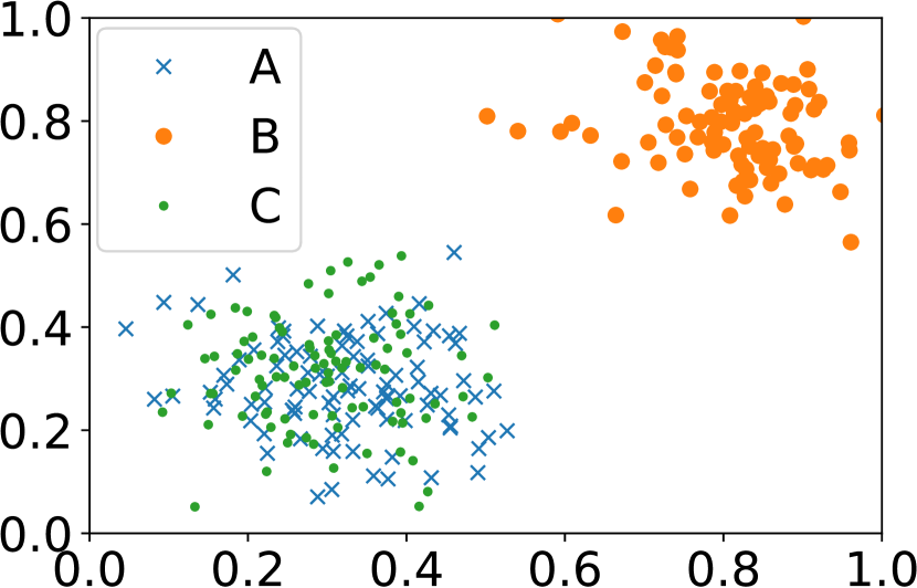
(a) $A$, $B$, $C$ columns in original space.

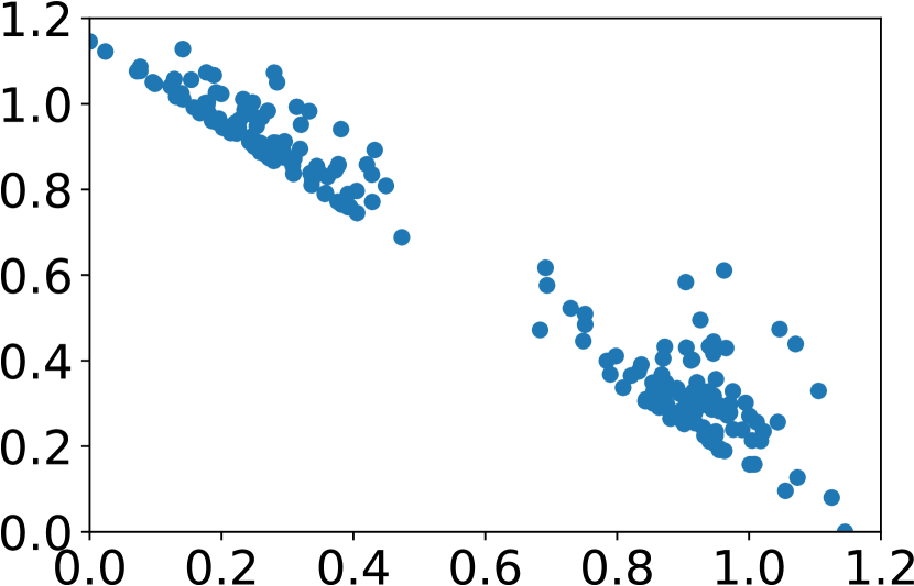
(b) Pivot mapping $A$ and $B$ columns.

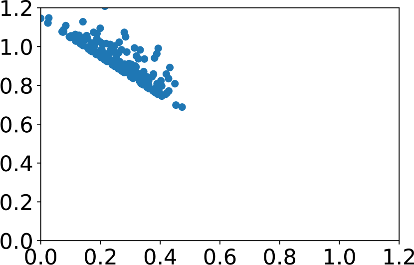
(c) Pivot mapping $A$ and $C$ columns.

Figure 5: Pivot mapping with different groupings.

A common scenario is that the number of columns extracted from the data lake is extremely large, and we cannot load all the data in a single PEXESO and hold them in main memory. Nonetheless, PEXESO is flexible in the sense that we can split the data into small partitions and each partition is indexed in a PEXESO framework. When processing a joinable table search, we load each partition into main memory at a time and search the results, and merge the results from from every PEXESO to obtain the final ones.

An important problem is how to make a good partition that can maximizes the power of each PEXESO. To this end, we propose a data partitioning method based on a clustering with Jensen–Shannon divergence.

Recall in Section III-D, pivots are selected from outliers. One observation is that if we group columns with different data distributions, the power of selected pivots will decline. For example, there are three columns $A$, $B$, and $C$ in Fig. 5(a). $A$ has a similar distribution to $C$, and $B$ has a different distribution from them. If we group $A$ and $B$ together and select the pivots from them, the outliers in $A$ are far away from those in $B$, and the pre-computed distances will be not helpful to the pivot-based filtering of the vectors in $B$, and vice versa. On the other hand, if we group similar columns $A$ and $C$ together, the outliers in $A$ can also work for the vectors in $B$. Figs. 5(b) and 5(c) are the pivot mapping result for $\{\,A,B\,\}$ and $\{\,A,C\,\}$, respectively. The white space is the filtered region. Obviously, grouping $\{\,A,C\,\}$ leads to better filter power than grouping $\{\,A,B\,\}$. Inspired by this observation, we choose to cluster the columns according to the similarity between distributions. KL divergence is a widely-used measure of such (dis)similarity. Since KL divergence is an asymmetric measure, we use the symmetric Jensen–Shannon divergence (JSD), a distance metric based on KL divergence.

$$JSD(A||B)=\frac{KLD(A||B)+KLD(B||A)}{2},$$

where $KLD(A||B)=\sum_{x\in X}A(x)\cdot log(\frac{A(x)}{B(x)})$.

We propose a clustering algorithm, which follows the $k$-means clustering paradigm. (1) Since JSD is a measure between probability distributions, we summarize a column of vectors with a probability distribution histogram composed of a number of bins, i.e., to obtain the statistics of the probability of points in a space region. (2) We randomly select $k$ columns as the center of $k$ clusters. (3) For each column (as a histogram), we compute the JSD distance to all the $k$ centers, and assign this column to the cluster that yields the minimum JSD. (4) For each cluster, we compute the mean of the histograms in this cluster and update the center. (5) Steps (2) – (4) are repeated until reaching a user-defined iteration number $t$. The time complexity of the algorithm is $O(|R|\cdot k\cdot t)$.

V Specifying Thresholds for Joinable Table Search

We discuss how to specify the two thresholds in our PEXESO framework. In general, we can convert the thresholds to ratios so users are able to specify them in an intuitive way, irrespective of data types, embedding approaches, or query column size.

• For distance threshold $\tau$, we first normalize all the vectors to unit length. The maximum possible distance between any two vectors is thus fixed (e.g., 2 for Euclidean distance). Then we set the threshold as a percentage of the maximum distance: a larger percentage indicates a looser matching condition and may increase the number of retrieved joinable columns.

• For joinability threshold $T$, we set it as a percentage of the query column size. A larger percentage means a smaller number of retrieved joinable columns.

VI Experiments

VI-A Setting

Datasets. We use the following datasets. Table III summarizes the statistics, including the number of vectors, the number of string columns, the average number of vectors per column, the pre-trained model used to embed strings, and the dimensionality. (1) OPENis a dataset of relational tables from Canadian Open Data Repository [39]. We extract English tables that contain more than 10 rows. We transform the values to 300-dimensional vectors with fastText [9]. (2) WDCis the WDC Web Table Corpus [28]. We use the English relational Web tables 2015. String values are split into English words and GloVe [12] is used to transform each word to a 50-dimensional vector. Then we compute the average of the word embeddings. We extract two subsets of this dataset, denoted by SWDC (small WDC, for in-memory) and LWDC (large WDC, for out-of-core), respectively.

For each dataset, we randomly sample 50 (for effectiveness) or 100 (for efficiency) tables from the dataset as query tables and removed it from the dataset to avoid duplicate result. We use Euclidean distance for the distance function $d(\cdot,\cdot)$. $\tau$ varies from 2% to 8% maximum distance (i.e., 2 for normalized vectors, see Section V), and the default value is 6%. $T$ varies from 20% to 80% query column size, and the default value is 60%.

To construct the table repository, we load raw tabular data stored in CSV format and extract the columns that are possible to be join keys. The WDC dataset contains the key column information. For the datasets without such information, we use the SATO method [35] to detect data types in tables and chose the columns whose types (e.g., names) can serve as a join key. Note that only string columns are involved in the evaluation because the other columns (e.g., IDs) in the datasets can be either dealt with equi-join, which has been addressed in [37], or do not produce meaningful join results. We also remove tables that are vertical, lack key column information, or contain less than five rows.

Competitors. For effectiveness, we compare equi-join [37], Jaccard-join (using Jaccard simialrity to match records), edit-join (using edit distance to match records), fuzzy-join [32], TF-IDF-join [6], and our PEXESO. For efficiency, we consider the following competitors. (1) PEXESOis our proposed method. (2) PEXESO-Hhas the same hierarchical grid-based blocking as PEXESO but replaces the inverted index-based verification with a naive method: for each candidate pair, it computes the distance for the query vector and every vector in the cell. (3) CTREEis an exact method using cover tree [14]. It builds a cover tree index for all the vectors and issues a range query with radius $\tau$ for each vector in the query column. Then each result of the range query is counted towards the joinability of the column it belongs to. We use the implementation in [31]. (4) EPTis an exact method using a pivot table [29], which was suggested in [4] for its competitiveness in most cases. It follows the same workflow as CTREE but replaces the cover tree with a pivot table. We implement it by ourselves. (5) PQis an approximate method. It follows the same workflow as CTREE but process the range query with product quantization [16]. We use the nanopq implementation [23]. Like PEXESO, we also equip the other methods with early termination in verification: when we increment the joinability counter of a column, if the count reaches $T$, then the column becomes joinable and we can skip it for further verification.

TABLE III: Dataset statistics.

Dataset	# Tab.	# Vec.	# Col.	Avg. Vec./Col.	Model	Dim.
OPEN	10.2K	17.2M	21.6K	796	fastText	300
SWDC	516K	8.6M	516K	16.7	GloVe	50
LWDC	48.9M	602M	48.9M	12.3	GloVe	50

TABLE IV: Precision & recall of joinable table search.

	OPEN		SWDC
Methods	Precision	Recall	Precision	Recall
equi-join	1.000	0.611	1.000	0.589
Jaccard-join	0.876	0.732	0.919	0.781
edit-join	0.814	0.756	0.833	0.842
fuzzy-join	0.834	0.795	0.865	0.833
TF-IDF-join	0.784	0.712	0.810	0.782
PEXESO	0.911	0.821	0.948	0.868
our join with PQ-85	0.787	0.422	0.744	0.461

Environments. Experiments are run on a server with a 2.20GHz Intel Xeon CPU E7-8890 and 630 GB RAM. All the competitors are implemented in Python 3.7.

TABLE V: Performance in ML tasks.

(a) Company classification.

Method	# Match	Micro-F1
no-join	-	$0.825\pm 0.057$
equi-join	0.13%	$0.806\pm 0.069$
Jaccard-join	0.54%	$0.816\pm 0.075$
fuzzy-join	0.83%	$0.836\pm 0.083$
edit-join	0.88%	$0.831\pm 0.063$
TF-IDF-join	0.72%	$0.826\pm 0.083$
PEXESO	0.76%	$\boldsymbol{0.855\pm 0.045}$

(b) Amazon toy product classification.

Method	# Match	Micro-F1
no-join	-	$0.589\pm 0.077$
equi-join	0.09%	$0.586\pm 0.051$
Jaccard-join	0.56%	$0.585\pm 0.073$
fuzzy-join	0.83%	$0.592\pm 0.055$
edit-join	0.89%	$0.596\pm 0.067$
TF-IDF-join	0.82%	$0.594\pm 0.049$
PEXESO	0.76%	$\boldsymbol{0.613\pm 0.072}$

(c) Video game sale regression.

Method	# Match	MSE
no-join	-	$2.10\pm 0.75$
equi-join	0.05%	$2.09\pm 0.65$
Jaccard-join	0.14%	$2.05\pm 0.73$
fuzzy-join	0.28%	$1.98\pm 0.61$
edit-join	0.53%	$2.01\pm 0.83$
TF-IDF-join	0.31%	$2.02\pm 0.55$
PEXESO	0.64%	$\boldsymbol{1.78\pm 0.66}$

VI-B Effectiveness of Joinable Table Search

We first evaluate the effectiveness on OPEN and SWDC. We randomly sample 50 tables from each dataset as query table and specify a key column in each of them as query column. We request our colleagues of database researchers to label whether a retrieved table is joinable. Precision and recall are measured. Precision $=$ (# retrieved joinable tables) $/$ (# retrieved tables). Since it is too laborious to label every table in the dataset, we follow [15] and build a retrieved pool using the union of the tables identified by the competitors: Recall $=$ (# retrieved joinable tables) $/$ (# joinable tables in the retrieved pool).

The thresholds of each competitor are tuned for highest F1 score. Table IV reports the average results. Equi-join has 100% precision, but its recall is significantly lower than the other methods. Jaccard-join has higher precision than fuzzy-join but its recall is lower. PEXESO delivers the highest recall, and the advantage over equi-join and Jaccard-join is remarkable. PEXESO also outperforms Jaccard-join and fuzzy-join in precision, and achieves over 90% precision on both datasets. This showcases that PEXESO finds more joinable tables than other options and most of its identified tables are really joinable. Besides, in order to explain why choose an exact solution to the joinable table search problem, we replace our algorithm with an approximate method of product quantization to find matching vectors and tune its recall of range query to 85%. Such modification (dubbed “our join with PQ-85”) results in low precision and recall, meaning that using an approximate solution to find matching vectors is not a good option.

VI-C Performance Gain in ML Tasks

We evaluate three ML tasks to show the usefulness of joinable table discovery. The columns are embedded using fastText [9]. For the query table in each task, we sample 1,000 records and search for joinable tables in the SWDC dataset that serves as a data lake. Then we left-join the query table to the identified joinable tables. Due to the noise in SWDC, a column is discarded if the size (excluding missing values) is smaller than 200. There are two types of possible conflicts in the join results: first, one record in the query column may match multiple records in a target column; second, since we join query table with all the identified joinable tables, these target tables may share the same column. The first type of conflict is not observed in this experiment. To address the second type, we aggregate the values of the columns with similar column names by string concatenation and summing up numerical values. Recursive feature elimination is applied on the join results to select meaningful features. With these features, a random forest model is trained for testing the prediction accuracy. In addition to the aforementioned competitors, we also consider using the query table without joins (referred to as “no-join”). We measure micro-F1 score for classification and mean squared error (MSE) for regression. Parameters are tuned to avoid overfitting. The best average scores of a 4-fold cross-validation are reported.

Company classification. We use the company information table [17] which contains 73,935 companies with 13 classes of categories (professional services, healthcare, etc.). The task is to predict the category of each company. We use “company_name” as query column. Table V(a) reports the average micro-F1 score and the number of records in the data lake identified as match to those in the query table. Equi-join only finds 0.13% matching records in the data lake, and compared to no-join, it worsens the performance for the ML task, because the few identified results make the joined table sparse and cause overfitting. Despite more records marked as match by fuzzy-join and edit-join, many of them are false positives. PEXESO achieves the highest F1 score with +0.019 performance gain over the runner-up.

Amazon toy product classification. The dataset contains 10,000 rows of toy products from Amazon.com [18]. The task is to predict the category from 39 classes (hobbies, office, arts, etc.) of each toy. We use “product_name” as query column. Table V(b) reports the average micro-F1 score and the data lake record marked as match. Similar results are witnessed as we have seen in company classification. PEXESO perform the best, reporting +0.017 performance gain over the runner-up.

Video game sales regression. The dataset contains 11,493 rows of video games with attributes and sales information [19]. The task is to predict the global sales. We use “Name” (game’s name) as query column. Table V(c) reports the average MSE and the data lake record marked as match. Compared to no-join, all the other methods improve the performance. PEXESO reports the lowest MSE and reduces it by 10% from the runner-up.

The above tasks show that joining tables with open data enhances the accuracy and our semantic-aware solution yields more gains. Note we do not join with open data blindly. It is also important to perform feature selection over the joined results.

TABLE VI: Parameter tuning in PEXESO.

		OPEN Time (s)			SWDC Time (s)
$|P|$	$m$	index	block	block + verify	index	block	block + verify
1	2	456.2	1.12	123.5	301.6	0.12	16.4
1	4	464.1	1.25	142.5	302.9	0.10	15.2
1	6	466.9	1.73	179.2	315.2	0.19	15.2
1	8	458.2	2.12	196.9	301.9	0.25	16.0
3	2	477.9	1.17	145.9	412.3	0.17	12.9
3	4	482.6	1.30	166.1	421.0	0.15	12.8
3	6	481.7	1.25	89.7	451.9	0.20	16.3
3	8	489.7	1.26	127.6	507.1	0.22	21.1
5	2	483.7	1.09	78.7	448.5	0.15	12.7
5	4	478.8	1.23	58.0	468.3	0.17	14.2
5	6	527.9	1.25	41.8	520.8	0.19	18.4
5	8	537.5	1.08	68.6	595.5	0.23	23.2
7	2	579.9	1.18	95.4	518.0	0.11	14.8
7	4	602.6	1.16	81.0	568.3	0.13	15.7
7	6	647.2	1.05	54.0	619.3	0.15	17.9
7	8	765.7	1.56	62.4	695.6	0.24	20.0
9	2	788.5	1.13	74.3	571.0	0.13	18.0
9	4	863.0	1.16	69.8	610.7	0.11	18.0
9	6	899.8	1.09	67.9	690.6	0.23	21.3
9	8	865.3	1.17	85.4	758.4	0.27	22.3

TABLE VII: Efficiency evaluation (OPEN and SWDC are in-memory; LWDC is out-of-core; program is terminated if processing time exceeded 2 hours).

		OPEN Search Time (s)				SWDC Search Time (s)				LWDC Search Time (s)
$T$	$\tau$	CTREE	EPT	PEXESO-H	PEXESO	CTREE	EPT	PEXESO-H	PEXESO	CTREE	EPT	PEXESO-H	PEXESO
20%	2%	678	710	75.4	32.5	678	691	130	9.8	$>$ 7200	$>$ 7200	3567	456
20%	4%	656	794	88.6	35.9	778	739	131	10.2	$>$ 7200	$>$ 7200	4156	468
20%	6%	706	888	157	33.7	599	683	134	10.2	$>$ 7200	$>$ 7200	4678	475
20%	8%	795	973	244	47.5	567	696	133	10.6	$>$ 7200	$>$ 7200	4532	474
40%	2%	811	711	66.7	33.0	766	642	136	13.6	$>$ 7200	$>$ 7200	5678	514
40%	4%	897	793	99.5	44.1	787	655	140	13.6	$>$ 7200	$>$ 7200	5895	556
40%	6%	899	884	165	42.4	767	678	134	11.6	$>$ 7200	$>$ 7200	6892	578
40%	8%	905	967	277	54.0	789	672	143	12.0	$>$ 7200	$>$ 7200	6245	602
60%	2%	867	704	74.8	42.2	677	577	137	12.8	$>$ 7200	$>$ 7200	5786	598
60%	4%	913	796	106	52.6	767	768	156	12.5	$>$ 7200	$>$ 7200	5409	601
60%	6%	922	884	177	51.8	745	726	157	12.8	$>$ 7200	$>$ 7200	6789	603
60%	8%	932	957	279	52.1	766	715	150	13.0	$>$ 7200	$>$ 7200	$>$ 7200	623
80%	2%	910	712	81.3	51.5	776	809	138	13.2	$>$ 7200	$>$ 7200	6157	635
80%	4%	898	780	108	53.4	813	823	134	13.4	$>$ 7200	$>$ 7200	6245	622
80%	6%	903	907	199	59.1	823	817	152	13.4	$>$ 7200	$>$ 7200	$>$ 7200	627
80%	8%	934	913	266	68.1	831	829	157	13.6	$>$ 7200	$>$ 7200	$>$ 7200	628

VI-D Parameter Tuning for Efficiency

There are two parameters in PEXESO: $|P|$, the number of pivots, and $m$, the number of levels in the hierarchical grids. Table VI shows the index construction time, the blocking time, and the total search time (i.e., blocking and verification) with varying $|P|$ and $m$ on OPEN and SWDC. The latter two are averaged over 1,000 queries. The optimal parameters are $|P|=5$ and $m=6$ for OPEN and $|P|=3$ and $m=4$ for SWDC. We choose these parameters as the default setting. Next we discuss the two parameters respectively.

Varying $|P|$. When we increase the pivot size, the index construction spends more time. The search time first drops and then rebounds. This is because a larger pivot set filters more vectors but increases the number of cells in the hierarchical grids and cause more candidate pairs in the form of (vector, cell).

Varying $m$. The effect of $m$ is similar to that of $|P|$. This is because a larger $m$ yields finer granularity of the hierarchical grids and improves the filtering power, while it results in more overhead for inverted index access.

Justification of cost analysis. We also evaluate the optimal $m$ obtained by our cost analysis (Section III-E). The optimal $m$ obtained by analysis is 5 (4.4 before ceiling) on OPEN and 4 (3.7 before ceiling) on SWDC, while the empirically optimal values are 6 and 4 on the two datasets, respectively. This suggests that our analysis is effective in PEXESO’s index construction. In addition, the result in Table VI shows that the blocking time is negligible in the overall search time, which justifies our assumption for the cost analysis.

VI-E Efficiency Evaluation

Performance on in-memory search. Table VII (left 2/3 part) summarizes the search time for the in-memory case on OPEN and SWDC, averaged over 1,000 queries. PEXESO performs the best in all the cases. It is 14 to 76 times faster than the non-blocking methods and 1.6 to 13 times faster than PEXESO-H.

Varying $\tau$. From Table VII, we also observe the search time trends with varying distance threshold $\tau$. In general, the search time increases with $\tau$. This is because the range query condition becomes looser. For example, for CTREE, a larger $\tau$ causes more overlapping tree nodes; for PEXESO, more candidates survive the filtering of hierarchical grids.

Varying $T$. We observe the search time generally increases with $T$ from Table VII. The reason is that the methods are equipped with the early termination technique such that whenever the joinability counter reaches $T$, the column is immediately confirmed as joinable. When $T$ increases, this early termination becomes less effective and results in more search time. Nonetheless, PEXESO is less vulnerable to this effect due to its inverted index-based verification.

Distance computation. To better understand why PEXESO is faster, we plot the number of distance computations in Fig. 6(a). PEXESO reports far less times of distance computation than the other options. The result also shows that our blocking is useful in reducing distance computation, as PEXESO-H also reports less distance computation times than the other baselines.

Index size. Fig. 6(b) shows the index size comparison. Albeit highest, the index size of PEXESO is only 2 times CTREE or EPT. Considering the significant speedup we have witnessed, it is worth spending moderately more space. Moreover, most memory consumption is the table repository storage.

Performance on out-of-core search. We partition the LWDC dataset into 10 parts with the JSD clustering (Section IV). The index is in-memory and the dataset is disk-resident. Table VII (right 1/3 part) reports the search time, which includes the overhead of loading the data from disks. Note that we report the time only if it is within 2 hours. PEXESO is still the fastest, and it is 8 to 11 times faster than PEXESO-H.

Pivot selection and data partitioning. To show the PCA-based pivot selection is a good choice, we compare with a baseline that randomly selects data points from the dataset. Fig. 7(a) reports the difference. The PCA-based method is overwhelmingly better, especially when there are more vectors in the dataset. To evaluate the proposed partitioning algorithm, we sample from LWDC 10,000 tables with 32,549 columns. We partition the set of columns with the proposed JSD clustering, random partitioning, and average $k$-means clustering (i.e., regarding each column as the average of its vectors and running a $k$-means clustering). Fig. 7(b) shows the search time with varying number of clusters. The proposed method is consistently better: it is 1.4 to 1.6 times faster than random partitioning and 1.1 to 1.2 times faster than average $k$-means clustering.

Comparison with approximate method. We compare PEXESO with an approximate method of product quantization (PQ). We adjust PQ to make the recall of range query at least 75% and 85% and denote the resultant method PQ-75 and PQ-85, respectively. Fig. 8 plots the search time on SWDC. PEXESO is competitive with PQ-85, and it is even faster than PQ-75 and PQ-85 when $T$ is 20% query column size.

Ablation study. We divide the lemmata into four groups and remove each group at a time. Fig. 9 shows how they affect search time. The filtering ones (Lemmata 1, 3, and 4) are more effective than their matching counterparts (Lemmata 2, 5, and 6). The group of vector-cell (Lemma 3) and cell-cell (Lemma 4) filtering is by far the most effective. This suggests that our filtering principles developed upon hierarchical grids are more effective than the point-wise ones used in existing work [4].

Scalability evaluation. We vary the number of columns, the number of vectors, and the dimensionality of embeddings to evaluate the scalability of PEXESO. To vary the number of columns, we uniformly sample columns from the table repository. To vary the number of vectors, we do not sample from the collection of vectors but uniformly sample a percentage of rows from each column. Figs. 10(a) – 10(e) plot the search time and index size on out-of-core LWDC, where only PEXESO and PEXESO-H are shown because the other methods are too slow. When varying the number of columns or vectors, PEXESO’s search time and index size scale almost linearly while PEXESO-H reports superlinear growth. The reason is PEXESO utilizes an inverted index-based verification technique which reduces the number of vector pairs for distance computation to almost linear. The search times of both methods scale almost linearly with the dimensionality of embeddings. This is because the distance computation is linear in the dimensionality, and it dominates the overall search time. Their index sizes do not change with the dimensionality because they are constructed for the pivot space.

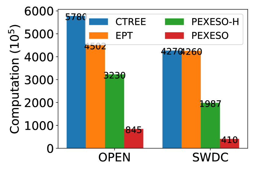
(a) Distance computation times.

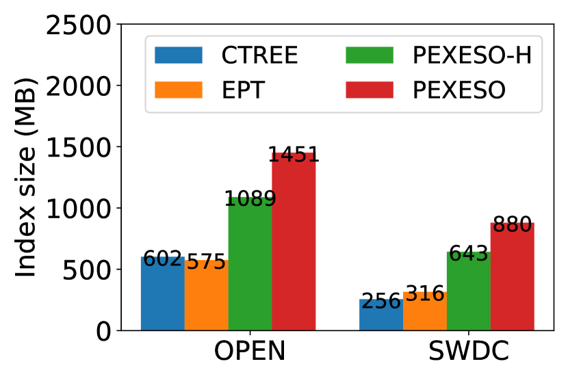
(b) Index size.

Figure 6: Distance computation and index size (OPEN and SWDC).

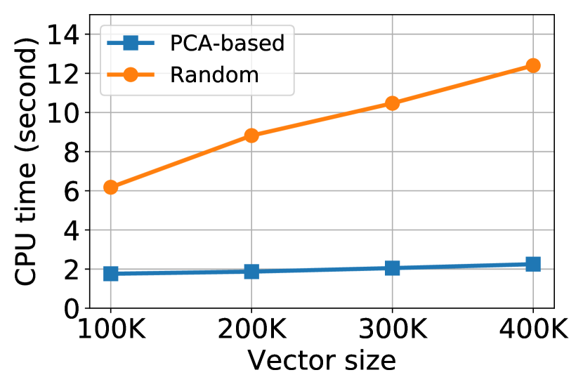
(a) Pivot selection algorithms.

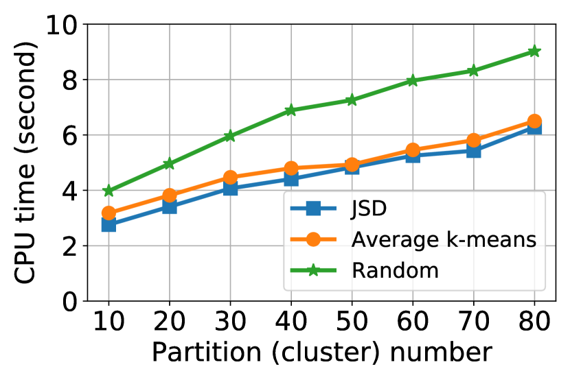
(b) Data partitioning algorithms.

Figure 7: Pivot selection and data partitioning (LWDC).

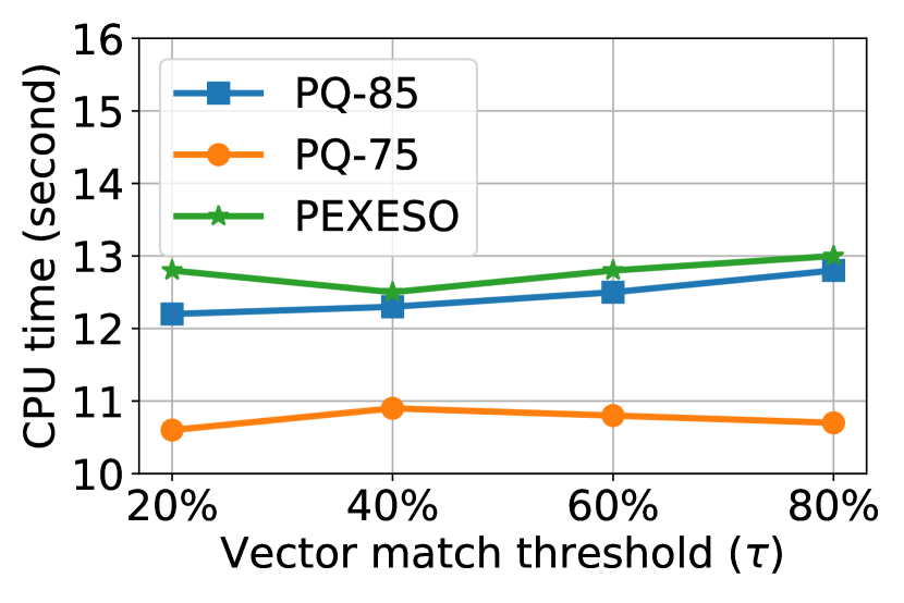
(a) Varying $\tau$.

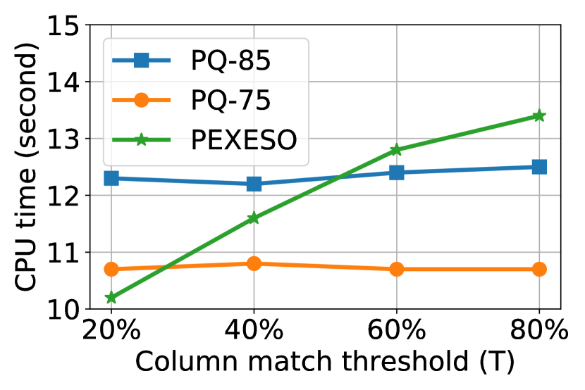
(b) Varying $T$.

Figure 8: Comparison to approximate method PQ (SWDC).

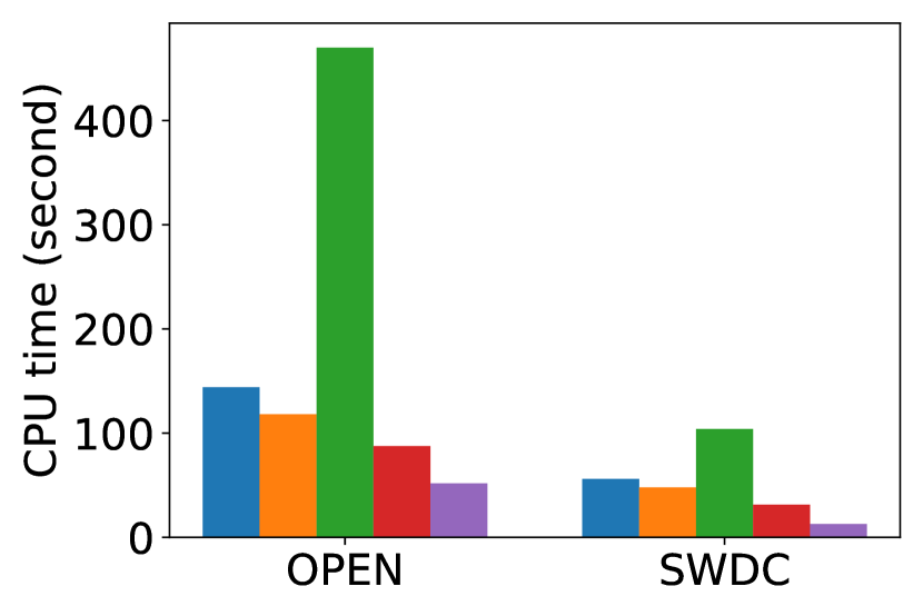
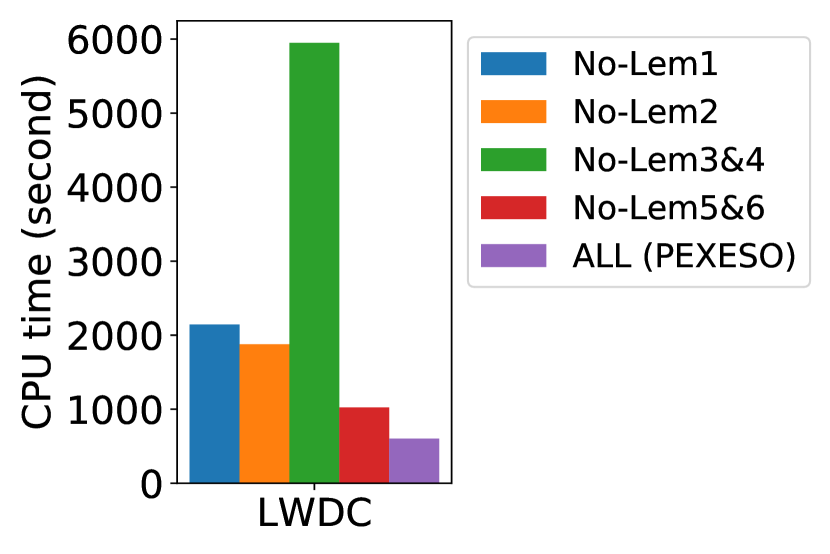
Figure 9: Ablation study (OPEN, SWDC, and LWDC).

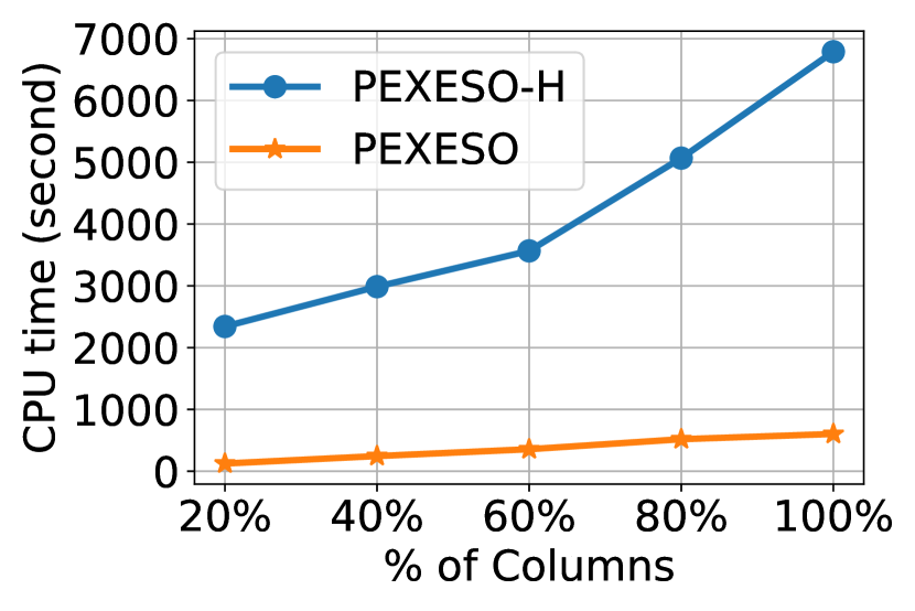
(a) Varying % of columns.

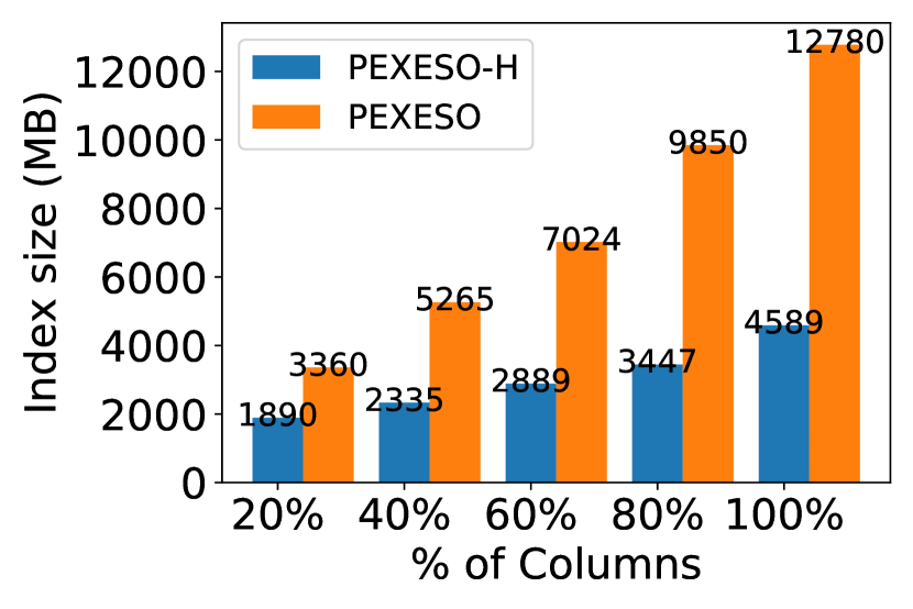
(b) Varying % of columns.

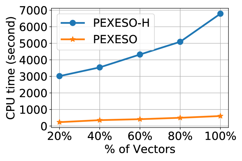
(c) Varying % of vectors.

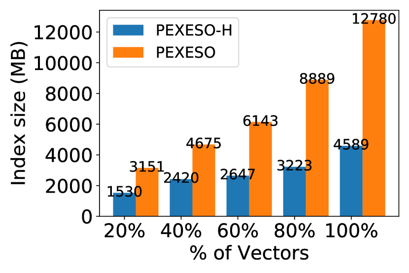
(d) Varying % of vectors.

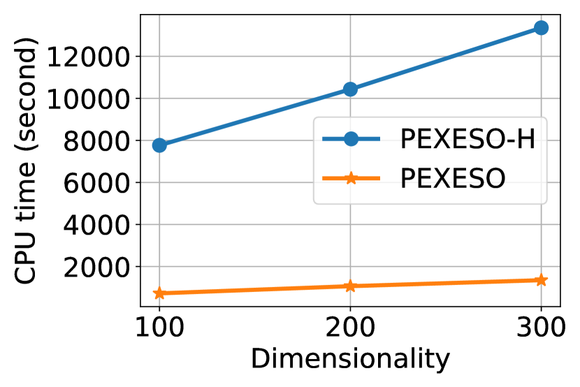
(e) Varying dimensinality.

Figure 10: Scalability evaluation (LWDC).

VII Related Work

Related table discovery. Besides joinable table search [37, 39], there are studies on finding related tables with criteria other than joinability. Nargesian et al. [25] developed LSH-based techniques for searching unionable tables, i.e., searching in a data lake for columns that can be vertically concatenate to a query table. Zhang and Ives studied related table discovery with a composite score of multiple similarities [36]. Bogatu et al. [1] also proposed a scoring function involving multiple attributes of a table and studied on finding top-$k$ results.

Similarity in metric space. There has been plenty of work in this area. We refer readers to [26] for a recent survey. The most related ones to our work are: Yu et al. [34] applied the iDistance technique to $k$NN join. Fredriksson and Braithwaite [11] improved the quick join algorithm for similarity joins. Pivot-based methods were surveyed in [4, 3]. These methods answer similarity queries but cannot solve our problem efficiently for the following reasons: (1) the indexing methods rebuild the index when the threshold changes and they also need an index for the query column, and (2) the non-indexing methods deal with one-time joins, whereas joinable table search may be invoked multiple times in a data lake. We utilize a hierarchical grid to partition the pivot space and develop filtering conditions and verification techniques specific to our problem.

Joining related tables. Set and string similarities have also been used to find related tables. For query processing algorithms, we refer readers to [21] for experimental comparison and [27] for recent advances. Wang et al. designed a fuzzy join predicate that combines token and characters and proposed the corresponding algorithm [32]. Deng et al. [8] studied the related set (table) search problem that finds sets with the maximum bipartite matching metrics. Wang et al. proposed MF-join [33] that performs a fuzzy match with multi-level filtering. The above solutions were not designed for data lakes (see [37]) and only deal with raw textual data rather than high-dimensional vectors. Zhu et al. proposed auto-join [38], which joins two tables with string transformations on columns. He et al. proposed SEMA-join [13], which finds related pairs between two tables with statistical correlation. Although optimizations for joining two given tables were introduced in the two studies, when applying to our problem, it is prohibitive to try joining every table in the data lake with the query table.

VIII Conclusion

We studied the problem of joinable table discovery in data lakes. We proposed the PEXESO framework which utilizes pre-trained models to transform textual attributes to high-dimensional vectors so that records can be semantically joined via similarity predicates and more meaningful results can be identified. To speed up the search process, we designed an indexing method along with a block-and-verify algorithm based on pivot-based filtering. We proposed a partitioning method to handle the out-of-core case for very large data lakes. The experiments showed that PEXESO outperforms alternative solutions in finding joinable tables, and the identified tables improve the performance of building ML models. The experiments also demonstrated the superiority of PEXESO in efficiency.

References

- [1] A. Bogatu, A. A. A. Fernandes, N. W. Paton, and N. Konstantinou. Dataset discovery in data lakes. In ICDE, pages 709–720, 2020.
- [2] A. Z. Broder, D. Carmel, M. Herscovici, A. Soffer, and J. Y. Zien. Efficient query evaluation using a two-level retrieval process. In CIKM, pages 426–434, 2003.
- [3] L. Chen, Y. Gao, X. Li, C. S. Jensen, and G. Chen. Efficient metric indexing for similarity search and similarity joins. IEEE Trans. Knowl. Data Eng., 29(3):556–571, 2017.
- [4] L. Chen, Y. Gao, B. Zheng, C. S. Jensen, H. Yang, and K. Yang. Pivot-based metric indexing. PVLDB, 10(10):1058–1069, 2017.
- [5] N. Chepurko, R. Marcus, E. Zgraggen, R. C. Fernandez, T. Kraska, and D. Karger. ARDA: automatic relational data augmentation for machine learning. PVLDB, 13(9):1373–1387, 2020.
- [6] W. W. Cohen. Integration of heterogeneous databases without common domains using queries based on textual similarity. In SIGMOD, pages 201–212, 1998.
- [7] D. Deng, R. C. Fernandez, Z. Abedjan, S. Wang, M. Stonebraker, A. K. Elmagarmid, I. F. Ilyas, S. Madden, M. Ouzzani, and N. Tang. The data civilizer system. In CIDR, 2017.
- [8] D. Deng, A. Kim, S. Madden, and M. Stonebraker. Silkmoth: An efficient method for finding related sets with maximum matching constraints. PVLDB, 10(10):1082–1093, 2017.
- [9] Facebook AI Research Lab. fastText: Library for efficient text classification and representation learning. https://fasttext.cc/, 2020.
- [10] R. C. Fernandez, E. Mansour, A. A. Qahtan, A. K. Elmagarmid, I. F. Ilyas, S. Madden, M. Ouzzani, M. Stonebraker, and N. Tang. Seeping semantics: Linking datasets using word embeddings for data discovery. In ICDE, pages 989–1000, 2018.
- [11] K. Fredriksson and B. Braithwaite. Quicker similarity joins in metric spaces. In SISAP, pages 127–140, 2013.
- [12] GloVe. Glove: Global vectors for word representation. https://nlp.stanford.edu/projects/glove/, 2019.
- [13] Y. He, K. Ganjam, and X. Chu. SEMA-JOIN: joining semantically-related tables using big table corpora. PVLDB, 8(12):1358–1369, 2015.
- [14] M. Izbicki and C. R. Shelton. Faster cover trees. In ICML, pages 1162–1170, 2015.
- [15] C. S. J. and W. Peter. Estimating the recall performance of web search engines. Aslib Proceedings, 49(7):184–189, Jan 1997.
- [16] H. Jégou, M. Douze, and C. Schmid. Product quantization for nearest neighbor search. IEEE Trans. Pattern Anal. Mach. Intell., 33(1):117–128, 2011.
- [17] Kaggle. Company classification. https://www.kaggle.com/charanpuvvala/company-classification, 2020.
- [18] Kaggle. Toy products on amazon. https://www.kaggle.com/PromptCloudHQ/toy-products-on-amazon, 2020.
- [19] Kaggle. Video game sales. https://www.kaggle.com/gregorut/videogamesales, 2020.
- [20] A. Kumar, J. F. Naughton, and J. M. Patel. Learning generalized linear models over normalized data. In SIGMOD, pages 1969–1984, 2015.
- [21] W. Mann, N. Augsten, and P. Bouros. An empirical evaluation of set similarity join techniques. PVLDB, 9(9):636–647, 2016.
- [22] R. Mao, W. L. Miranker, and D. P. Miranker. Pivot selection: Dimension reduction for distance-based indexing. J. Discrete Algorithms, 13:32–46, 2012.
- [23] Y. Matsui. Nano product quantization. https://github.com/matsui528/nanopq, 2020.
- [24] S. Mudgal, H. Li, T. Rekatsinas, A. Doan, Y. Park, G. Krishnan, R. Deep, E. Arcaute, and V. Raghavendra. Deep learning for entity matching: A design space exploration. In SIGMOD, pages 19–34, 2018.
- [25] F. Nargesian, E. Zhu, K. Q. Pu, and R. J. Miller. Table union search on open data. PVLDB, 11(7):813–825, 2018.
- [26] J. Qin, W. Wang, C. Xiao, and Y. Zhang. Similarity query processing for high-dimensional data. PVLDB, 13(12):3437–3440, 2020.
- [27] J. Qin and C. Xiao. Pigeonring: A principle for faster thresholded similarity search. PVLDB, 12(1):28–42, 2018.
- [28] D. Ritze, O. Lehmberg, R. Meusel, C. Bizer, and S. Zope. WDC web table corpus. http://webdatacommons.org/webtables/2015/downloadInstructions.html, 2015.
- [29] G. Ruiz, F. Santoyo, E. Chávez, K. Figueroa, and E. S. Tellez. Extreme pivots for faster metric indexes. In SISAP, pages 115–126, 2013.
- [30] W. Tao, D. Deng, and M. Stonebraker. Approximate string joins with abbreviations. PVLDB, 11(1):53–65, 2017.
- [31] P. Varilly. Coveratree. https://github.com/patvarilly/CoverTree, 2020.
- [32] J. Wang, G. Li, and J. Feng. Extending string similarity join to tolerant fuzzy token matching. ACM Trans. Database Syst., 39(1):7:1–7:45, 2014.
- [33] J. Wang, C. Lin, and C. Zaniolo. Mf-join: Efficient fuzzy string similarity join with multi-level filtering. In ICDE, pages 386–397, 2019.
- [34] C. Yu, B. Cui, S. Wang, and J. Su. Efficient index-based KNN join processing for high-dimensional data. Information & Software Technology, 49(4):332–344, 2007.
- [35] D. Zhang, Y. Suhara, J. Li, M. Hulsebos, Ç. Demiralp, and W. Tan. Sato: Contextual semantic type detection in tables. PVLDB, 13(11):1835–1848, 2020.
- [36] Y. Zhang and Z. G. Ives. Finding related tables in data lakes for interactive data science. In SIGMOD, pages 1951–1966, 2020.
- [37] E. Zhu, D. Deng, F. Nargesian, and R. J. Miller. JOSIE: overlap set similarity search for finding joinable tables in data lakes. In SIGMOD, pages 847–864, 2019.
- [38] E. Zhu, Y. He, and S. Chaudhuri. Auto-join: Joining tables by leveraging transformations. PVLDB, 10(10):1034–1045, 2017.
- [39] E. Zhu, F. Nargesian, K. Q. Pu, and R. J. Miller. LSH ensemble: Internet-scale domain search. PVLDB, 9(12):1185–1196, 2016.