Revisiting convolutional neural network on graphs with polynomial approximations of Laplace-Beltrami spectral filtering

Abstract

This paper revisits spectral graph convolutional neural networks (graph-CNNs) given in Defferrard (2016) and develops the Laplace-Beltrami CNN (LB-CNN) by replacing the graph Laplacian with the LB operator. We then define spectral filters via the LB operator on a graph. We explore the feasibility of Chebyshev, Laguerre, and Hermite polynomials to approximate LB-based spectral filters and define an update of the LB operator for pooling in the LB-CNN. We employ the brain image data from Alzheimer’s Disease Neuroimaging Initiative (ADNI) and demonstrate the use of the proposed LB-CNN. Based on the cortical thickness of the ADNI dataset, we showed that the LB-CNN didn’t improve classification accuracy compared to the spectral graph-CNN. The three polynomials had a similar computational cost and showed comparable classification accuracy in the LB-CNN or spectral graph-CNN. Our findings suggest that even though the shapes of the three polynomials are different, deep learning architecture allows us to learn spectral filters such that the classification performance is not dependent on the type of the polynomials or the operators (graph Laplacian and LB operator).

Declarations

Funding

This research/project is supported by the National Science Foundation MDS-2010778, National Institute of Health R01 EB022856, EB02875, and National Research Foundation, Singapore under its AI Singapore Programme (AISG Award No: AISG-GC-2019-002). Additional funding is provided by the Singapore Ministry of Education (Academic research fund Tier 1; NUHSRO/2017/052/T1-SRP-Partnership/01), NUS Institute of Data Science. This research was also supported by the A*STAR Computational Resource Centre through the use of its high-performance computing facilities.

Conflicts of interest/Competing interests

The authors declare that they have no conflict of interest.

Availability of data and material

Data used in preparation of this article were obtained from the Alzheimer’s Disease Neuroimaging Initiative (ADNI) database (adni.loni.ucla.edu).

Code availability

https://bieqa.github.io/deeplearning.html

1 Introduction

Graph convolutional neural networks (graph-CNNs) are deep learning techniques that apply to graph-structured data. Graph-structured data are in general complex, which imposes significant challenges on existing convolutional neural network algorithms. Graphs are irregular and have variable number of unordered vertices with different topology at each vertex. This makes important algebraic operations such as convolutions and pooling challenging to apply to the graph domain. Hence, existing research on graph-CNN has been focused on defining convolution and pooling operations.

There are two types of approaches for defining convolution on a graph: one through the spatial domain and the other through the spectral domain Bronstein et al. (2017); Zhang et al. (2020). Existing spatial approaches, such as diffusion-convolutional neural networks (DCNNs) Atwood and Towsley (2015), PATCHY-SAN Niepert et al. (2016); Duvenaud et al. (2015), gated graph sequential neural networks Li et al. (2015), DeepWalk Perozzi et al. (2014), message-passing neural network (MPNN) Gilmer et al. (2017), develop convolution in different ways to process the vertices on a graph whose neighborhood has different sizes and connections. An alternative approach is to take into account of the geometry of a graph and to map individual patches of a graph to a representation that is more amenable to classical convolution, including 2D polar coordinate representation Masci et al. (2015), local windowed spectral representation Boscaini et al. (2015), anisotropic variants of heat kernel diffusion filters Boscaini et al. (2016b, a), Gaussian Mixture-model kernels Monti et al. (2016).

On the other hand, several graph-CNN methods called ”spectral graph-CNN” defines convolution in the spectral domainBruna et al. (2013); Defferrard et al. (2016); Henaff et al. (2015); Kipf and Welling (2016); Yi et al. (2017); Ktena et al. (2017); Shuman et al. (2016). The advantage of spectral graph-CNN methods lies in the analytic formulation of the convolution operation. Based on the spectral graph theory, Bruna et al. Bruna et al. (2013) proposed convolution on graph-structured data in the spectral domain via the graph Fourier transform. However, the eigendecomposition of the graph Laplacian for building the graph Fourier transform is computationally intensive when a graph is large. Moreover, spectral filters in Bruna et al. (2013) are non-localized in the spatial domain. Defferrard et al. Defferrard et al. (2016) addressed these problems by proposing Chebyshev polynomials to parametrize spectral filters such that the resulting convolution is approximated by the polynomials of the graph Laplacian. Kipf and Welling Kipf and Welling (2016) adopted the first-order polynomial filter and stacked more spectral convolutional layers to replace higher-order polynomial expansions. In Defferrard et al. (2016); Shuman et al. (2016), it is shown that the $k$-order Chebyshev polynomial approximation of graph Laplacian filters performs the $k$-ring filtering operation.

In this study, we revisited the spectral graph-CNN based on the graph Laplacian Defferrard et al. (2016); Shuman et al. (2016) and developed the LB-CNN where spectral filters are designed via the Laplace-Beltrami (LB) operator on a graph. We call these filters as LB-based spectral filters. We investigated whether the proposed LB-CNN is superior to the graph-CNN Defferrard et al. (2016); Shuman et al. (2016) because the LB operator incorporates the intrinsic geometry of a graph better than graph Laplacian Perrault-Joncas et al. (2017). We further explored the feasibility of Chebyshev, Laguerre, and Hermite polynomials to approximate LB-based spectral filters in the LB-CNN. We chose Laguerre and Hermite polynomials beyond Chebyshev polynomials since these polynomials have potentials to approximate the heat kernel convolution on a graph as shown in Tan and Qiu (2015); Huang et al. (2020). We employed the brain image data from Alzheimer’s Disease Neuroimaging Initiative (ADNI) and demonstrated the use of the proposed LB-CNN. We compared the computational time and classification performance of the LB-CNN with the spectral graph-CNN Defferrard et al. (2016); Shuman et al. (2016) when Chebyshev, Laguerre, and Hermite polynomials were used.

This study contributes to

• providing the approximation of LB spectral filters using Chebyshev, Laguerre, Hermite polynomials and their implementation in the LB-CNN;

• updating the LB operator for pooling in the LB-CNN;

• demonstrating the feasibility of using the LB operator and different polynomials for graph-CNNs.

2 Methods

Similar to classical CNN and spectral graph-CNN Defferrard et al. (2016), the LB-CNN has three major components, including convolution, rectified linear unit (ReLU), and pooling. In the following, we will first describe LB spectral filters in the convolutional layer and how to define a pooling operation via coarsening a graph and updating the LB operator.

2.1 Laplace-Beltrami spectral filters

2.1.1 Polynomial approximation of LB spectral filters

Consider the Laplace-Beltrami (LB) operator $\Delta$ on surface $\mathcal{M}$. Let $\psi_{j}$ be the $j^{th}$ eigenfunction of the LB-operator with eigenvalue $\lambda_{j}$

$${\Delta}\psi_{j}=\lambda_{j}\psi_{j}\ ,$$ (1)

where $0=\lambda_{0}\leq\lambda_{1}\leq\lambda_{2}\leq\cdots$. A signal $f(x)$ on the surface $\mathcal{M}$ can be represented as a linear combination of the LB eigenfunctions

$$f(x)=\sum_{j=0}^{\infty}c_{j}\psi_{j}(x)\ ,$$ (2)

where $c_{j}$ is the $j^{th}$ coefficient associated with the eigenfunction $\psi_{j}(x)$.

We now consider an LB spectral filter $g$ on $\mathcal{M}$ with spectrum $g(\lambda)$ as

$$g(x,y)=\sum_{j=0}^{\infty}g(\lambda_{j})\psi_{j}(x)\psi_{j}(y).$$ (3)

Based on Eq. (2), the convolution of a signal $f$ with the filter $g$ can be written as

$$h(x)=g\ast f(x)=\sum_{j=0}^{\infty}g(\lambda_{j})c_{j}\psi_{j}(x).$$ (4)

As suggested in Defferrard et al. (2016); Wee et al. (2019); Coifman and Maggioni (2006); Hammond et al. (2011); Kim et al. (2012); Tan and Qiu (2015), the filter spectrum $g(\lambda)$ in Eq. (4) can be approximated as the expansion of Chebyshev polynomials, $T_{k}$, $k=0,1,2,\dots,K-1$, such that

$$g(\lambda)=\sum_{k=0}^{K-1}\theta_{k}T_{k}(\lambda)\ .$$ (5)

$\theta_{k}$ is the $k^{th}$ expansion coefficient associated with the $k^{th}$ Chebyshev polynomial. $T_{k}$ is the Chebyshev polynomial of the form $T_{k}(\lambda)=\cos(k\cos^{-1}\lambda)$. The left panel on Fig. 1 shows the shape of the $k^{th}$ Chebyshev polynomial up to order 6. We can rewrite the convolution in Eq. (4) as

$$h(x)=g\ast f(x)=\sum_{k=0}^{K-1}\theta_{k}T_{k}(\Delta)f(x).$$ (6)

Likewise, $g(\lambda)$ in Eq. (4) can also be approximated using other polynomials, such as Laguerre or Hermite polynomials Olver et al. (2010). $T_{k}$ in Eq. (6) can be replaced by Laguerre, $L_{k}$, or Hermite, $H_{k}$, polynomials, where

$$L_{k}(\lambda) =\sum_{l=0}^{k}\binom{k}{l}\frac{(-\lambda)^{l}}{l!},$$ (7)

$$H_{k}(\lambda) =k!\sum_{l=0}^{\lfloor k/2\rfloor}\frac{(-1)^{l}(2\lambda)^{k-2l}}{l!(k-2l)!}\ ,$$

In this paper, we adopt the following normalized definition of Hermite polynomials:

$$\bar{H}_{k}(\lambda)=\frac{1}{\sqrt{2^{k}k!}}H_{k}(\lambda)\,$$ (8)

where the inner product of $\bar{H}_{k}$ with itself is independent of $k$. The last two panels of Fig. 1 show the shapes of Laguerre and Hermite polynomials up to order 6, respectively.

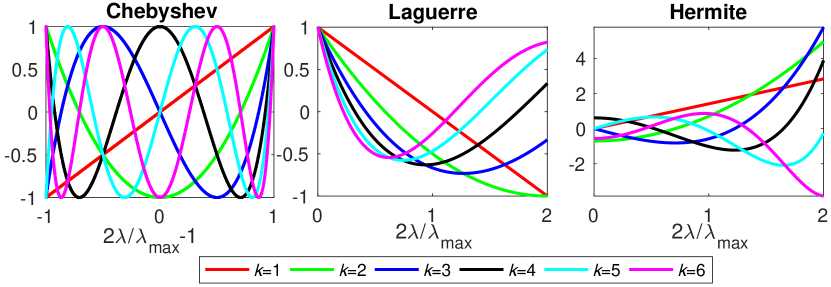
Figure 1: Chebyshev, Laguerre and Hermite polynomials of order from 1 to 6. The eigenvalues were scaled and shifted to $[-1,1]$ for Chebyshev polynomials and to $[0,2]$ for Laguerre and Hermite polynomials, where $\lambda_{\max}$ is the maximum eigenvalue of the LB-operator.

2.1.2 Numerical implementation of LB spectral filters via polynomial approximations

We now discretize the surface $\mathcal{M}$ as a triangulated mesh, $\mathcal{G}=\{V,E\}$, with a set of triangles and vertices $v_{i}$. For the implementation of the LB spectral filters, we adopt the discretization scheme of the LB operator in Tan and Qiu (2015). The $ij^{th}$ element of the LB-operator on $\mathcal{G}$ can be computed as

$$\Delta_{ij}=C_{ij}/A_{i},$$ (9)

where $A_{i}$ is estimated by the Voronoi area of nonobtuse triangles Meyer et al. (2003) and the Heron’s area of obtuse triangles containing $v_{i}$ Tan and Qiu (2015); Meyer et al. (2003). The off-diagonal entries are defined as $C_{ij}=-(\cot\theta_{ij}+\cot\phi_{ij})/2$ if $v_{i}$ and $v_{j}$ form an edge, otherwise $C_{ij}=0$. The diagonal entries $C_{ii}$ are computed as $C_{ii}=-\sum_{j}C_{ij}$. Other cotan discretizations of the LB operator are discussed in Chung and Taylor (2004); Qiu et al. (2006); Chung et al. (2015). When the number of vertices on $\mathcal{M}$ is large, the computation of the LB eigenfunctions can be costly Huang et al. (2020).

For the sake of simplicity, we denote the $k^{th}$ order polynomial as $P_{k}$, where $P_{k}$ can represent Chebyshev, Laguerre, or Hermite polynomial. We take the advantage of the recurrence relation of these polynomials (Table 1) and compute LB spectral filters recursively as follows.

• compute $\Delta$ based on Eq. (9) for the triangulated mesh $\mathcal{G}$;

• compute the maximum eigenvalue $\lambda_{\max}$ of $\Delta$. For the standardization across surface meshes, we normalize $\Delta$ as $\widetilde{\Delta}=\frac{2\Delta}{\lambda_{\max}}-I$ such that the eigenvalues are mapped from $[0,\lambda_{\max}]$ to $[-1,1]$ for Chebyshev polynomials Defferrard et al. (2016); Huang et al. (2020). $I$ is an identity matrix. For Laguerre and Hermite polynomials, we normalize $\Delta$ as $\widetilde{\Delta}=\frac{2\Delta}{\lambda_{\max}}$, which maps the eigenvalues from $[0,\lambda_{\max}]$ to $[0,2]$;

• for a signal $f(x)$, compute $P_{k}(\widetilde{\Delta})f(x)$ recursively by

  $$P_{k+1}({\widetilde{\Delta}})f=A_{k}{\widetilde{\Delta}}\ P_{k}({\widetilde{\Delta}})f+B_{k}P_{k}({\widetilde{\Delta}})f+C_{k}P_{k-1}({\widetilde{\Delta}})f,$$ (10)

  with the initial conditions $P_{-1}({\widetilde{\Delta}})f(x)=0$ and $P_{0}({\widetilde{\Delta}})f(x)=f(x)$. The recurrence relations of different polynomials are given in Table 1.

Step 3 is repeated from $k=0$ till $k=K-2$.

Table 1: The recurrence relation of Chebyshev, Laguerre and Hermite polynomials in spectral filtering.

Method	Recurrence relations
Chebyshev†	$T_{k+1}(\widetilde{\Delta})f=(2-\delta_{k0})\widetilde{\Delta}\ T_{k}(\widetilde{\Delta})f-T_{k-1}(\widetilde{\Delta})f$
Laguerre	$L_{k+1}(\widetilde{\Delta})f=\frac{-\widetilde{\Delta}\ L_{k}(\widetilde{\Delta})f+(2k+1)L_{k}(\widetilde{\Delta})f-kL_{k-1}(\widetilde{\Delta})f}{k+1}$
Hermite	$\bar{H}_{k+1}(\widetilde{\Delta})f=\sqrt{\frac{2}{k+1}}\widetilde{\Delta}\ \bar{H}_{k}(\widetilde{\Delta})f-\sqrt{\frac{k}{k+1}}\bar{H}_{k-1}(\widetilde{\Delta})f$

^† $\delta_{k0}$ is Kronecker delta.

2.1.3 Localization of spectral filters based on polynomial approximations

Analogue to the spatial localization property of Chebyshev polynomial approximation of graph Laplacian spectral filters Defferrard et al. (2016), we can show that Chebyshev, Laguerre, or Hermite polynomial approximation of LB spectral filters also has this localization property. We consider the discretization of $\Delta$ given in Eq. (9). Consider two vertices $v_{i}$ and $v_{j}$ on $\mathcal{G}$. We can define the shortest distance between $v_{i}$ and $v_{j}$, denoted by $d_{\mathcal{G}}(i,j)$, as the minimum number of edges on the path connecting $v_{i}$ and $v_{j}$. Hence,

$$(\Delta^{K})_{i,j}=0\ \ \textmd{ if }\ \ d_{\mathcal{G}}(i,j)>K,$$ (11)

where $\Delta^{K}$ denotes the $K$-th power of the LB operator $\Delta$ Tan and Qiu (2015). In other words, the coverage of $(\Delta^{K})_{i,j}$ is localized in the ball with radius $k$ from the central vertex.

$P_{k}(\Delta)$ can be represented in terms of $\Delta^{0},\Delta,\cdots,\Delta^{k}$ and is $k$-localized $(P_{k}(\Delta))_{i,j}=0$ if $d_{\mathcal{G}}(i,j)>k$ according to Eq. (11). The spectral filter $g$ composed of $P_{0}(\Delta)$, $P_{1}(\Delta)$, …, $P_{K-1}(\Delta)$ is a spatially localized filter with localization property given by

$$\left(g(\Delta)\right)_{i,j}=0\ \ \textmd{ if }\ \ d_{\mathcal{G}}(i,j)>K-1.$$ (12)

In practice, we can also show the spatial localization of filter $g$ composed of $P_{0}(\Delta)$, $P_{1}(\Delta)$, …, $P_{K-1}(\Delta)$ by applying $g$ to an impulse signal $f_{j}$ with $1$ at vertex $v_{j}$ and $0$ at the others. Then, the filter output is given by $g(x,v_{j})=\sum_{k=0}^{K-1}\theta_{k}P_{k}(\Delta)f_{j}(x)$. When $x=v_{i}$ satisfying $d_{\mathcal{G}}(i,j)>K-1$, since $(P_{k}(\Delta))_{i,j}=0$, we have

$$g(v_{i},v_{j})=\sum_{k=0}^{K-1}\theta_{k}\left(P_{k}(\Delta)f_{j}(x)\right)_{i}=\sum_{k=0}^{K-1}\theta_{k}\left(P_{k}(\Delta)\right)_{ij}=0.$$ (13)

2.2 Rectified Linear Unit

Similar to classic CNN, a rectified linear unit (ReLU) in the LB-CNN can be represented by many non-linear activation functions. The activation function is a map from ${\mathbb{R}}$ to ${\mathbb{R}}$, which does not involve any geometrical property of a triangulated mesh. In our proposed LB-CNN on a mesh, we adopt the well-known ReLU:

$$\sigma(z)=\max\{0,z\},\quad z\in{\mathbb{R}}.$$

2.3 Mesh coarsening and pooling

For the LB-CNN, the pooling layer involves mesh coarsening, pooling of signals, and an update of the LB operator. First, we adopt the Graclus multilevel clustering algorithm Dhillon et al. (2007) to coarsen a graph based on the graph Laplacian. This algorithm is built on the METIS Karypis and Kumar (1998) to cluster similar vertices together from a given graph by a greedy algorithm. At each coarsening level, two neighboring vertices with maximum local normalized cut are matched until all vertices are explored Shi and Malik (2000). In our case, the discrete LB-operator $\Delta$ in Eq. (9) is used. The local normalized cut on a mesh is computed by $-\Delta_{ij}(1/\Delta_{ii}+1/\Delta_{jj})$. The coarsening process is repeated until the coarsest level is achieved. After coarsening, a balanced binary tree is generated where each node has either one (i.e. singleton) or two child nodes. Fake nodes are added to pair with those singleton. The weights of the edges involving fake nodes are set as 0. Then, the pooling on this binary tree can be efficiently implemented as a simple 1-dimensional pooling of size 2.

We now discuss the update of the LB operator for a coarsen mesh. When two matched nodes are merged together at a coarser level, the weights of the edges involving the two nodes are merged by summing them together. By doing so, each coarsened mesh has its updated $\Delta$.

2.4 LB-CNN Architecture

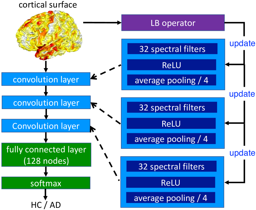
Figure 2: An example of LB-CNN architectures for the classification of health controls (HC) and Alzheimer’s Disease (AD) patients. The cortical surface is represented as a triangulated mesh with 655,360 triangles and 327,684 vertices.

We are now well equipped with all the components for a LB-CNN network. The LB-CNN network is composed of total $L+1$ connected stages. The first $L$ stages are the stages for feature extraction. Each stage contains three sequentially concatenated layers: (1) a convolutional layer with multiple LB spectral filters; (2) a ReLU layer; (3) a pooling layer with stride 2 or higher that uses average pooling. In the last stage, a fully connected layer followed by a softmax function is employed to make a decision, and the output layer contains classification labels.

Fig. 2 illustrates one of LB-CNN architectures that are analogous to classical CNN for image data defined on equi-spaced grids. In this example, the $i$-th convolution layer is composed of $2^{i+2}$ LB spectral filters that can be approximated using Chebyshev, Laguerre, and Hermite polynomials, an ReLU, and an average pooling with pooling size $2^{\max\{5-i,1\}}$ and stride being the same as the pooling size. In the fully connected layer, there are $128$ hidden nodes, and an $l_{2}$-norm regularization with weight of $5\times 10^{-4}$ is applied to prevent overfitting.

All the networks can be trained by the back propagation algorithm with $30$ epochs, mini-batch size of $32$, initial learning rate of $10^{-3}$, learning rate decay of $0.05$ for every $20$ epochs, momentum of $0.9$ and no dropout.

2.5 MRI data acquisition and preprocessing

We utilized the structural T1-weighted MRI from the ADNI-2 cohort (adni.loni.ucla.edu). The aim of this study was to illustrate the use of the LB-CNN and spectral graph-CNN via the HC/AD classification since it has been well studied using T1-weighted image data (e.g., Cuingnet et al. (2011); Liu et al. (2013); Hosseini-Asl et al. (2016); Korolev et al. (2017); Liu et al. (2018); Islam and Zhang (2018); Basaia et al. (2019); Wee et al. (2019)). Hence, this study involved 643 subjects with HC or AD scans (392 subjects had HC scans; 253 subjects had AD scans). There were 8 subjects who fell into both groups due to the conversion from HC to AD. There were total 1122 scans for HC and 587 for AD.

The MRI data of the ADNI-2 cohort were acquired from participants aging from 55 to 90 years using either 1.5 or 3T scanners. The T1-weighted images were segmented using FreeSurfer (version 5.3.0) Fischl et al. (2002). The white and pial cortical surfaces were generated at the boundary between white and gray matter and the boundary of gray matter and CSF, respectively. Cortical thickness was computed as the distance between the white and pial cortical surfaces. It represents the depth of the cortical ribbon. We represented cortical thickness on the mean surface, the average between the white and pial cortical surfaces. We employed large deformation diffeomorphic metric mapping (LDDMM) Zhong et al. (2010); Du et al. (2011) to align individual cortical surfaces to the atlas and transferred the cortical thickness of each subject to the atlas. The cortical atlas surface was represented as a triangulated mesh with 655,360 triangles and 327,684 vertices. At each surface vertex, a spline regression implemented by piecewise step functions James et al. (2013) was performed to regress out the effects of age and gender. The residuals from the regression were used in the below spectral graph-CNN and LB-CNN.

3 Results

3.1 Spatial localization of the LB spetral filters via polynomial approximations

Fig. 3 shows the localization property of spectral filters using the Chebyshev, Laguerre and Hermite polynomials. The input signal is 1 at only one vertex and 0 at all other vertices of the hippocampus. The $P_{k}(\Delta)$ is strictly localized in a ball of radius $k$, i.e., $k$ rings from the central vertex. Fig. 4

Consider a signal having 1 on a small patch (see the first panel in Fig. 4) and 0 on the rest of a hippocampus surface mesh with 1184 vertices and 2364 triangles. Fig. 4 shows the convolutions of this signal with spectral filters $g=T_{k}$, $L_{k}$ or $\bar{H}_{k}$ for $k=1,4,7,10$. The spectral filters designed by different polynomials show different impacts on the signal in the spatial domain.

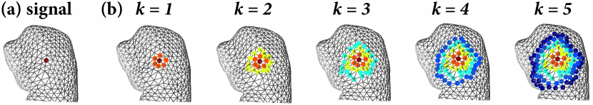
Figure 3: The first panel shows the signal with 1 at one vertex and 0 at the other vertices of the hippocampus. The rest of panels shows the spatial localization of spectral filters using Chebyshev $T_{k}$, Laguerre $L_{k}$ and Hermite $\bar{H}_{k}$ polynomials for $k=1,2,...,5$.

Figure 4: The first panel shows the input signal, where 1 is on a red region and 0 on the rest of the hippocampus. The rest panels show the signals after filtering via LB spectral filters, $g=T_{k}$, $L_{k}$ and $\bar{H}_{k}$ for $k=1,4,7,10$, where $T_{k}$, $L_{k}$ and $\bar{H}_{k}$ are the Chebyshev, Laguerre, and Hermite polynomials, respectively.

3.2 Comparison of spectral graph-CNN and LB-CNN

Table 2: Classification performance of the spectral graph-CNN and LB-CNN with Chebyshev, Laguerre, and Hermite polynomial approximations.

Spectral CNN	Polynomial	Layer	$K$	ACC (%)	SEN (%)	SPE (%)	GMean (%)
Graph	Chebyshev	4	6	$89.8\pm 0.4$	$90.1\pm 0.9$	$89.6\pm 0.6$	$89.9\pm 0.4$
	Laguerre	5	7	$90.0\pm 0.5$	$91.7\pm 1.1$	$89.2\pm 0.6$	$90.4\pm 0.6$
	Hermite	3	7	$87.1\pm 0.5$	$86.6\pm 1.6$	$87.4\pm 0.9$	$87.0\pm 0.7$
LB	Chebyshev	5	7	$90.9\pm 0.6$	$91.3\pm 0.1$	$90.7\pm 0.5$	$91.0\pm 0.7$
	Laguerre	5	7	$91.0\pm 0.4$	$91.2\pm 0.9$	$90.9\pm 0.8$	$91.1\pm 0.4$
	Hermite	4	7	$88.2\pm 0.6$	$87.5\pm 0.6$	$88.4\pm 1.1$	$88.0\pm 0.4$

ACC: accuracy; SEN: sensitivity; SPE: specificity; GMean: geometric mean.

We aimed to compare the computational cost and classification accuracy of the spectral graph-CNN Defferrard et al. (2016); Wee et al. (2019) and LB-CNN on the cortical thickness of the HC and the AD patients while Chebyshev, Laguerre and Hermite polynomials were used to approximate spectral filters.

In our experiments, the architecture of the spectral graph-CNN and LB-CNN was the same as shown in Fig. 2 except the number of layers. Ten-fold cross-validation was applied to the dataset (HC: $n=1122$; AD: $n=587$). One fold of real data was left out for testing. The remaining nine folds were further separated into training ($75\%$) and validation ($25\%$) sets randomly. To prevent potential data leakage in the ten-fold cross-validation, we constructed non-overlap training, validation, and testing sets with respect to subjects instead of MRI scans. This ensured that the scans from the same subjects were in the same set. The above data splitting was done for the HC and AD groups separately so that the ratio of the number of subjects in the two groups was similar in all sets.

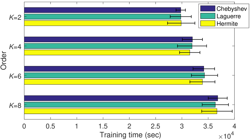
Figure 5: Computational cost of the LB-CNN using Chebyshev (blue), Laguerre (green) and Hermite (yellow) approximations of different order $K$. The ten-fold cross-validation was repeated for 10 times. The average and standard deviation of the training time are shown.

3.2.1 Computational Cost

The computation cost of the LB-CNN was similar to that of the spectral graph-CNN since they only differ on the edge weights between vertices. For instance, when the network with 3 convolutional layers and 6-order Hermite approximation was used, the spectral graph-CNN and LB-CNN respectively had training time $33625\pm 1310$ sec and $33908\pm 2385$ sec over the ten-fold cross validation with no significant difference (two-sample $t$-test $p=0.75$).

Next, we compared the computational cost of the LB-CNN with 3 convolutional layers using different polynomial approximations. Fig. 5 shows the training time of the LB-CNNs using the Chebyshev, Laguerre and Hermite approximation of order $K=2$, $4$, $6$ and $8$. Regardless of which polynomial was used, the training time increased as $K$ increased since more trainable parameters were needed to characterize the spectral filters. Given $K$, the three polynomial approximation methods had similar computation cost ($p>0.56$).

3.2.2 Classification Performance

To compare classification performance of the spectral graph-CNN and LB-CNN on HC and AD, the number of convolutional layers and polynomial approximation order were tuned for each CNN independently to achieve the best classification accuracy and geometric mean (GMean) on the validation set. The spectral graph-CNNs with Chebyshev, Laguerre and Hermite approximations respectively required 4 convolutional layers with polynomial order of $K=6$, 5 layers with $K=7$, and 3 layers with $K=7$. The LB-CNNs with Chebyshev and Laguerre approximations needed 5 layers with $K=7$ while the LB-CNN with Hermite approximation required 4 layers with $K=7$. Table 2 lists the accuracy, sensitivity, specificity and GMean of all these CNNs in classifying AD and HC.

Two-sample $\it{t}$-test found no significant difference in classification accuracy between the spectral graph-CNN and LB-CNN. For instance, when Chebyshev polynomials were used to approximate the spectral filters, the spectral graph-CNN classification accuracy was $89.9\%$ while the LB-CNN classification accuray was $90.9\%$ ($p=5.4\times 10^{-5}$). Likewise, there were no group differences in classification accuracy between the spectral graph-CNN and LB-CNN when Laguerre and Hermite polynomial approximations were used (Laguerre: $p=3.5\times 10^{-4}$; Hermite:$p=9.5\times 10^{-4}$). Hence, the LB- CNN classification performance can be viewed as equivalent to the spectral graph-CNN.

As for the comparisons among the three different polynomials, the classification performance of the Laguerre approximation was comparable to the Chebyshev approximation (graph-CNN: $p=0.27$; LB-CNN: $p=0.81$). However, the classification performance of both Chebyshev and Laguerre polynomial approximations was greater than that of the Hermite polynomial approximation (all $p<5.4\times 10^{-10}$). In Huang et al. (2020), Hermite polynomial approximation shows slower convergence to heat kernel, compared to Chebyshev and Laguerre polynomial approximations.

4 Discussions

In this study, we revisited the spectral graph-CNN Defferrard et al. (2016); Shuman et al. (2016) and developed the LB-CNN by replacing the graph Laplacian by the LB operator. We also employed Chebyshev, Laguerre, and Hermite polynomials to approximate the LB spectral filters in the LB-CNN and spectral graph-CNN. Based on cortical thickness of the ADNI dataset, we showed that the LB-CNN didn’t improve classification accuracy compared to the spectral graph-CNN Defferrard et al. (2016); Shuman et al. (2016). The three polynomials had the similar computational cost and showed comparable classification accuracy in the LB-CNN or spectral graph-CNN Defferrard et al. (2016); Shuman et al. (2016). Our findings suggest that even though the shapes of the three polynomials are different, deep learning architecture allows to learn spectral filters such that the classification performance is not dependent on the type of the polynomials or the operators (graph Laplacian and LB operator).

References

- Atwood and Towsley (2015) Atwood J, Towsley D (2015) Diffusion-convolutional neural networks. arXiv preprint arXiv:151102136
- Basaia et al. (2019) Basaia S, Agosta F, Wagner L, Canu E, Magnani G, Santangelo R, Filippi M, Initiative ADN, et al. (2019) Automated classification of alzheimer’s disease and mild cognitive impairment using a single mri and deep neural networks. NeuroImage: Clinical 21:101645
- Boscaini et al. (2015) Boscaini D, Masci J, Melzi S, Bronstein MM, Castellani U, Vandergheynst P (2015) Learning class-specific descriptors for deformable shapes using localized spectral convolutional networks. Computer Graphics Forum 34(5):13–23
- Boscaini et al. (2016a) Boscaini D, Masci J, Rodoia E, Bronstein M (2016a) Learning shape correspondence with anisotropic convolutional neural networks. In: NIPS’16 Proceedings of the 30th International Conference on Neural Information Processing Systems, ACM, pp 3197–3205
- Boscaini et al. (2016b) Boscaini D, Masci J, Rodola E, Bronstein MM, Cremers D (2016b) Anisotropic diffusion descriptors. Computer Graphics Forum 35(2):431–441
- Bronstein et al. (2017) Bronstein M, Bruna J, LeCun Y, Szlam A, Vandergheynst P (2017) Geometric deep learning: going beyond euclidean data. IEEE Signal Processing Magazine 34(4):18–42
- Bruna et al. (2013) Bruna J, Zaremba W, Szlam A, LeCun Y (2013) Spectral networks and locally connected networks on graphs. arXiv preprint arXiv:13126203
- Chung and Taylor (2004) Chung M, Taylor J (2004) Diffusion smoothing on brain surface via finite element method. In: Proceedings of IEEE International Symposium on Biomedical Imaging (ISBI), vol 1, pp 432–435
- Chung et al. (2015) Chung M, Qiu A, Seo S, Vorperian H (2015) Unified heat kernel regression for diffusion, kernel smoothing and wavelets on manifolds and its application to mandible growth modeling in CT images. Medical Image Analysis 22:63–76
- Coifman and Maggioni (2006) Coifman RR, Maggioni M (2006) Diffusion wavelets. Applied and Computational Harmonic Analysis 21(1):53–94
- Cuingnet et al. (2011) Cuingnet R, Gerardin E, Tessieras J, Auzias G, Lehéricy S, Habert MO, Chupin M, Benali H, Colliot O (2011) Automatic classification of patients with Alzheimer’s disease from structural MRI: a comparison of ten methods using the ADNI database. Neuroimage 56(2):766–781
- Defferrard et al. (2016) Defferrard M, Bresson X, Vandergheynst P (2016) Convolutional neural networks on graphs with fast localized spectral filtering. In: Proceedings of the 30th International Conference on Neural Information Processing Systems, NIPS, pp 3844–3852
- Dhillon et al. (2007) Dhillon IS, Guan Y, Kulis B (2007) Weighted graph cuts without eigenvectors a multilevel approach. IEEE Transactions on Pattern Analysis and Machine Intelligence 29(11):1944–1957
- Du et al. (2011) Du J, Younes L, Qiu A (2011) Whole brain diffeomorphic metric mapping via integration of sulcal and gyral curves, cortical surfaces, and images. NeuroImage 56(1):162–173
- Duvenaud et al. (2015) Duvenaud DK, Maclaurin D, Aguilera-Iparraguirre J, Gomez-Bombarelli R, Hirzel T, Aspuru-Guzik A, Adams RP (2015) Convolutional networks on graphs for learning molecular fingerprints. arXiv preprint arXiv:150909292
- Fischl et al. (2002) Fischl B, Salat DH, Busa E, Albert M, Dieterich M, Haselgrove C, Van Der Kouwe A, Killiany R, Kennedy D, Klaveness S, et al. (2002) Whole brain segmentation: automated labeling of neuroanatomical structures in the human brain. Neuron 33(3):341–355
- Gilmer et al. (2017) Gilmer J, Schoenholz SS, Riley PF, Vinyals O, Dahl GE (2017) Neural message passing for quantum chemistry. arXiv preprint arXiv:170401212
- Hammond et al. (2011) Hammond DK, Vandergheynst P, Gribonval R (2011) Wavelets on graphs via spectral graph theory. Applied and Computational Harmonic Analysis 30(2):129 – 150
- Henaff et al. (2015) Henaff M, Bruna J, LeCun Y (2015) Deep convolutional networks on graph-structured data. arXiv preprint arXiv:150605163
- Hosseini-Asl et al. (2016) Hosseini-Asl E, Keynton R, El-Baz A (2016) Alzheimer’s disease diagnostics by adaptation of 3d convolutional network. In: 2016 IEEE International Conference on Image Processing (ICIP), IEEE, pp 126–130
- Huang et al. (2020) Huang SG, Lyu I, Qiu A, Chung MK (2020) Fast polynomial approximation of heat kernel convolution on manifolds and its application to brain sulcal and gyral graph pattern analysis. IEEE Transactions on Medical Imaging 39(6):2201–2212
- Islam and Zhang (2018) Islam J, Zhang Y (2018) Brain mri analysis for alzheimer’s disease diagnosis using an ensemble system of deep convolutional neural networks. Brain Informatics 5(2):2
- James et al. (2013) James G, Witten D, Hastie T, Tibshirani R (2013) An introduction to statistical learning, vol 112. Springer
- Karypis and Kumar (1998) Karypis G, Kumar V (1998) A fast and high quality multilevel scheme for partitioning irregular graphs. SIAM Journal on Scientific Computing 20(1):359–392
- Kim et al. (2012) Kim WH, Pachauri D, Hatt C, Chung MK, Johnson S, Singh V (2012) Wavelet based multi-scale shape features on arbitrary surfaces for cortical thickness discrimination. In: Advances in Neural Information Processing Systems, pp 1241–1249
- Kipf and Welling (2016) Kipf TN, Welling M (2016) Semi-supervised classification with graph convolutional networks. arXiv preprint arXiv:160902907
- Korolev et al. (2017) Korolev S, Safiullin A, Belyaev M, Dodonova Y (2017) Residual and plain convolutional neural networks for 3d brain mri classification. In: 2017 IEEE 14th International Symposium on Biomedical Imaging (ISBI 2017), IEEE, pp 835–838
- Ktena et al. (2017) Ktena SI, Parisot S, Ferrante E, Rajchl M, Lee M, Glocker B, Rueckert D (2017) Distance metric learning using graph convolutional networks: Application to functional brain networks. arXiv preprint arXiv:170302161
- Li et al. (2015) Li Y, Tarlow D, Brockschmidt M, Zemel R (2015) Gated graph sequence neural networks. arXiv preprint arXiv:151105493
- Liu et al. (2018) Liu M, Zhang J, Adeli E, Shen D (2018) Landmark-based deep multi-instance learning for brain disease diagnosis. Medical image analysis 43:157–168
- Liu et al. (2013) Liu X, Tosun D, Weiner MW, Schuff N, Initiative ADN, et al. (2013) Locally linear embedding (lle) for mri based alzheimer’s disease classification. Neuroimage 83:148–157
- Masci et al. (2015) Masci J, Boscaini D, Bronstein MM, Vandergheynst P (2015) Geodesic convolutional neural networks on riemannian manifolds. In: Computer Vision (ICCV), 2015 IEEE International Conference on, IEEE, p 832–840
- Meyer et al. (2003) Meyer M, Desbrun M, Schröder P, Barr AH (2003) Discrete differential-geometry operators for triangulated 2-manifolds. In: Visualization and mathematics III, Springer, pp 35–57
- Monti et al. (2016) Monti F, Boscaini D, Masci J, Rodolà E, Svoboda J, Bronstein MM (2016) Geometric deep learning on graphs and manifolds using mixture model cnns. arXiv preprint arXiv:161108402
- Niepert et al. (2016) Niepert M, Ahmed M, Kutzkov K (2016) Learning convolutional neural networks for graphs. In: Proceeding of the 33rd International Conference on Machine Learning, ACM, p 2014––2023
- Olver et al. (2010) Olver FWJ, Lozier DW, Boisvert RF, Clark CW (2010) NIST handbook of mathematical functions. Cambridge University Press
- Perozzi et al. (2014) Perozzi B, Al-Rfou R, Skiena S (2014) Deepwalk: Online learning of social representations. In: Proceedings of the 20th ACM SIGKDD, ACM, p 701–710
- Perrault-Joncas et al. (2017) Perrault-Joncas DC, Meilǎ M, McQueen J (2017) Improved graph laplacian via geometric consistency. In: Proceedings of the 31st International Conference on Neural Information Processing Systems, pp 4460–4469
- Qiu et al. (2006) Qiu A, Bitouk D, Miller M (2006) Smooth functional and structural maps on the neocortex via orthonormal bases of the Laplace-Beltrami operator. IEEE Transactions on Medical Imaging 25:1296–1396
- Shi and Malik (2000) Shi J, Malik J (2000) Normalized cuts and image segmentation. IEEE Transactions on Pattern Analysis and Machine Intelligence 22(8):888–905
- Shuman et al. (2016) Shuman DI, Ricaud B, Vandergheynst P (2016) Vertex-frequency analysis on graphs. Applied and Computational Harmonic Analysis 40(2):260–291
- Tan and Qiu (2015) Tan M, Qiu A (2015) Spectral Laplace-Beltrami wavelets with applications in medical images. IEEE Transactions on Medical Imaging 34:1005–1017
- Wee et al. (2019) Wee CY, Liu C, Lee A, Poh JS, Ji H, Qiu A, Initiative ADN (2019) Cortical graph neural network for AD and MCI diagnosis and transfer learning across populations. NeuroImage: Clinical 23:101929
- Yi et al. (2017) Yi L, Su H, Guo X, Guibas L (2017) Syncspeccnn: Synchronized spectral cnn for 3d shape segmentation. In: Computer Vision and Pattern Recognition (CVPR), Conference on, IEEE, pp 6584–6592
- Zhang et al. (2020) Zhang Z, Cui P, Zhu W (2020) Deep learning on graphs: A survey. IEEE Transactions on Knowledge and Data Engineering
- Zhong et al. (2010) Zhong J, Phua DYL, Qiu A (2010) Quantitative evaluation of lddmm, freesurfer, and caret for cortical surface mapping. Neuroimage 52(1):131–141