Causal Effects of Linguistic Properties

Abstract

We consider the problem of using observational data to estimate the causal effects of linguistic properties. For example, does writing a complaint politely lead to a faster response time? How much will a positive product review increase sales? This paper addresses two technical challenges related to the problem before developing a practical method. First, we formalize the causal quantity of interest as the effect of a writer’s intent, and establish the assumptions necessary to identify this from observational data. Second, in practice, we only have access to noisy proxies for the linguistic properties of interest—e.g., predictions from classifiers and lexicons. We propose an estimator for this setting and prove that its bias is bounded when we perform an adjustment for the text. Based on these results, we introduce TextCause, an algorithm for estimating causal effects of linguistic properties. The method leverages (1) distant supervision to improve the quality of noisy proxies, and (2) a pre-trained language model (BERT) to adjust for the text. We show that the proposed method outperforms related approaches when estimating the effect of Amazon review sentiment on semi-simulated sales figures. Finally, we present an applied case study investigating the effects of complaint politeness on bureaucratic response times.

1 Introduction

Social scientists have long been interested in the causal effects of language, studying questions like:

• How should political candidates describe their personal history to appeal to voters (Fong and Grimmer, 2016)?

• How can business owners write product descriptions to increase sales on e-commerce platforms (Pryzant et al., 2017, 2018a)?

• How can consumers word their complaints to receive faster responses (Egami et al., 2018)?

• What conversational strategies can mental health counselors use to have more successful counseling sessions (Zhang et al., 2020)?

To study the causal effects of linguistic properties, we must reason about interventions: what would the response time for a complaint be if we could make that complaint polite while keeping all other properties (topic, sentiment, etc.) fixed? Although it is sometimes feasible to run such experiments where text is manipulated and outcomes are recorded Grimmer and Fong (2020), analysts typically have observational data consisting of texts and outcomes obtained without intervention. This paper formalizes the estimation of causal effects of linguistic properties in observational settings.

Estimating causal effects from observational data requires addressing two challenges. First, we need to formalize the causal effect of interest by specifying the hypothetical intervention to which it corresponds. The first contribution of this paper is articulating the causal effects of linguistic properties; we imagine intervening on the writer of a text document and telling them to use different linguistic properties.

The second challenge of causal inference is identification: we need to express causal quantities in terms of variables we can observe. Often, instead of the true linguistic property of interest we have access to a noisy measurement called the proxy label. Analysts typically infer these values from text with classifiers, lexicons, or topic models Grimmer and Stewart (2013); Lucas et al. (2015); Prabhakaran et al. (2016); Voigt et al. (2017); Luo et al. (2019); Lucy et al. (2020). The second contribution of this paper is establishing the assumptions we need to recover the true effects of a latent linguistic property from these noisy proxy labels. In particular, we propose an adjustment for the confounding information in a text document and prove that this bounds the bias of the resulting estimates.

The third contribution of this paper is practical: an algorithm for estimating the causal effects of linguistic properties. The algorithm uses distantly supervised label propagation to improve the proxy label Zhur and Ghahramani (2002); Mintz et al. (2009); Hamilton et al. (2016), then BERT to adjust for the bias due to text Devlin et al. (2018); Veitch et al. (2020). We demonstrate the method’s accuracy with partially-simulated Amazon reviews and sales data, perform a sensitivity analysis in situations where assumptions are violated, and show an application to consumer finance complaints. Data and a package for performing text-based causal inferences is available at https://github.com/rpryzant/causal-text.

2 Causal Inference Background

Causal inference from observational data is well-studied (Pearl, 2009; Rosenbaum and Rubin, 1983, 1984; Shalizi, 2013). In this setting, analysts are interested in the effect of a treatment $T$ (e.g., a drug) on an outcome $Y$ (e.g., disease progression). For ease, we consider binary treatments. The average treatment effect (ATE) on the outcome $Y$ is,

$$\psi=\mathbb{E}\left[Y\,;\,\mathrm{do}(T=1)\right]-\mathbb{E}\left[Y\,;\,\mathrm{do}(T=0)\right],$$ (1)

where the operation $\mathrm{do}(T=t)$ means that we hypothetically intervene and set the treatment $T$ to some value (Pearl, 2009).

Typically, the ATE $\psi$ is not the simple difference in average conditional outcomes, $\mathbb{E}\left[Y\,|\,T=1\right]-\mathbb{E}\left[Y\,|\,T=0\right]$. This is because confounding variables $C$ are associated with both the treatment and outcome, inducing non-causal associations between them, referred to as open backdoor paths Pearl (2009). When all the confounding variables are observed, we can write the ATE in terms of observed variables using the backdoor-adjustment formula Pearl (2009),

$$\psi=\mathbb{E}_{C}\Big{[}\mathbb{E}\left[Y\,|\,T=1,C\right]-\mathbb{E}\left[Y\,|\,T=0,C\right]\Big{]}.$$ (2)

For example, if the confounding variable $C$ is discrete, we group the data into values of $C$, calculate the average difference in outcomes between the treated and untreated samples of each group, and take the average over groups.

3 Causal Effects of Linguistic Properties

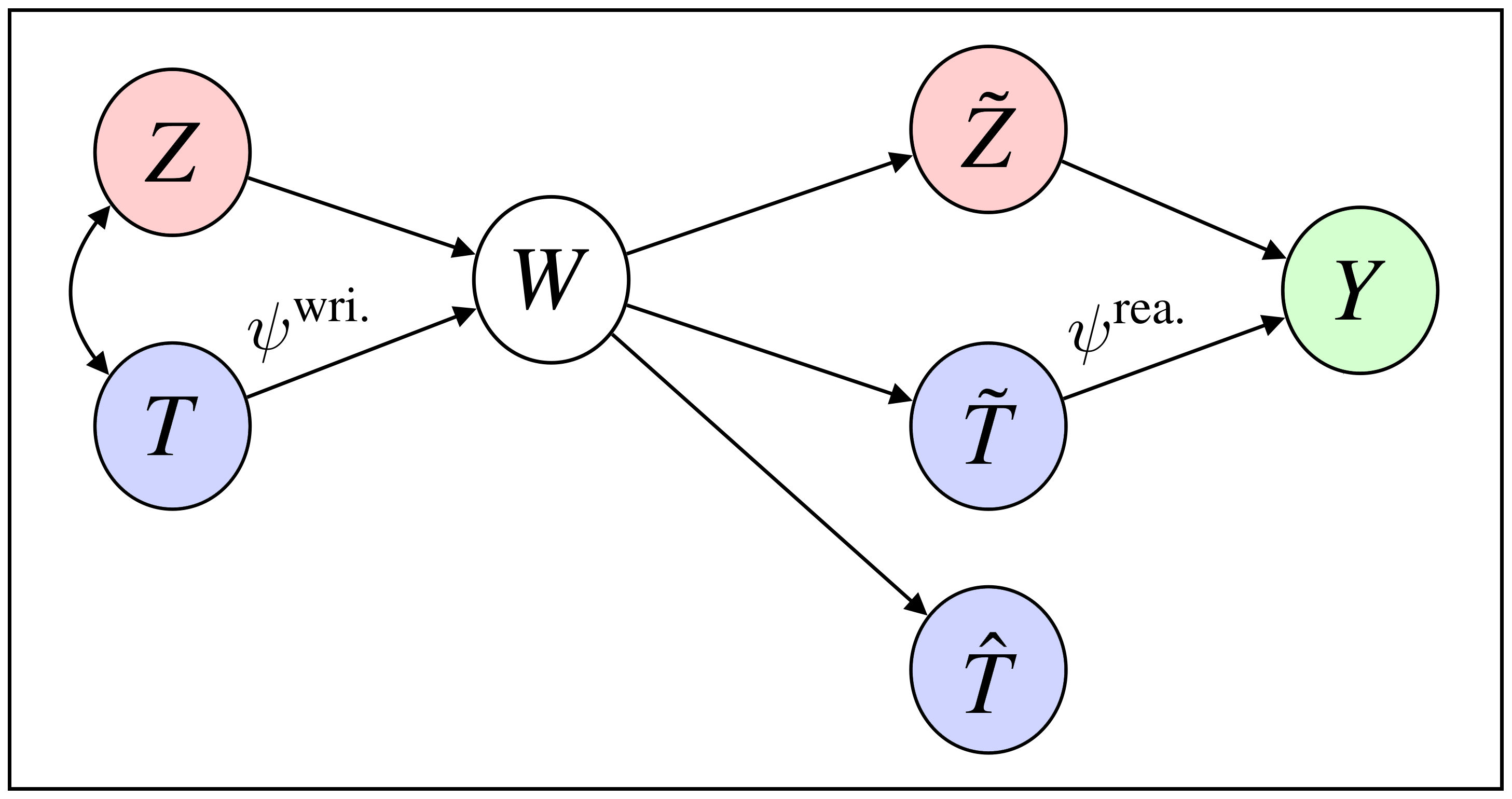
Figure 1: The proposed causal model of text and outcomes. A writer uses linguistic property $T$ and other properties $Z$, which may be correlated (denoted by bi-directed arrow), to write the text $W$. From the text, the reader perceives the property of interest, captured by $\tilde{T}$, and together with other perceived information $\tilde{Z}$, produces the outcome $Y$. The proxy label of the property obtained via a classifier or lexicon is captured by $\hat{T}$.

We are interested in the causal effects of linguistic properties. To formalize this as a treatment, we imagine intervening on the writer of a text, e.g., telling people to write with a property (or not). We show that to estimate the effect of using a linguistic property, we must consider how a reader of the text perceives the property. These dual perspectives of the reader and writer are well studied in linguistics and NLP; we adapt the idea for causal inference.

Figure 1 illustrates a causal model of the setting. Let $W$ be a text document and let $T$ (binary) be whether or not a writer uses a particular linguistic property of interest. For example, in consumer complaints, the variable $T$ can indicate whether the writer intends to be polite or not. The outcome is a variable $Y$, e.g., how long it took for this complaint to be serviced. Let $Z$ be other linguistic properties that the writer communicated (consciously or unconsciously) via the text $W$, e.g. topic, brevity or sentiment. The linguistic properties $T$ and $Z$ are typically correlated, and both variables affect the outcome $Y$.

We are interested in the average treatment effect,

$$\psi^{\textrm{wri.}}=\mathbb{E}\left[Y\,;\,\mathrm{do}(T=1)\right]-\mathbb{E}\left[Y\,;\,\mathrm{do}(T=0)\right],$$ (3)

where we imagine intervening on writers and telling them to use the linguistic property of interest (setting $T=1$, “write politely”) or not ($T=0$). This causal effect is appealing because the hypothetical intervention is well-defined – it corresponds to an intervention we could perform in theory. However, without further assumptions, $\psi^{\textrm{wri.}}$ is not identified from the observational data. The reason is that we would need to adjust for the unobserved linguistic properties $Z$, which create open backdoor paths because they are correlated with both the treatment $T$ and outcome $Y$ (Figure 1).

To solve this problem, we observe that the reader is the one who produces outcomes. Readers use the text $W$ to perceive a value for the property of interest (captured by the variable $\tilde{T}$) as well as other properties (captured by $\tilde{Z}$) then produce the outcome $Y$ based on these perceived values. For example, a customer service representative reads a consumer complaint, judges whether (among other things) the complaint is polite or not, and chooses how quickly to respond based on this.

Consider the average treatment effect,

$$\psi^{\textrm{rea.}}=\mathbb{E}\left[Y\,;\,\mathrm{do}(\tilde{T}=1)\right]-\mathbb{E}\left[Y\,;\,\mathrm{do}(\tilde{T}=0)\right],$$ (4)

where we imagine intervening on the reader’s perception of a linguistic property $\tilde{T}$. The following result shows that we can identify the causal effect of interest, $\psi^{\textrm{wri.}}$, by exploiting this ATE $\psi^{\textrm{rea.}}$.

Theorem 1.

Let $\tilde{Z}=f(W)$ be a function of the words $W$ such that $\mathbb{E}\left[Y\,|\,W\right]=\mathbb{E}\left[Y\,|\,\tilde{T},\tilde{Z}\right]$. Suppose that the following assumptions hold:

1. (no unobserved confounding) $W$ blocks backdoor paths between $\tilde{T}$ and $Y$,

2. (agreement of intent and perception) $T=\tilde{T}$.

3. (overlap) For some constant $\epsilon>0$,

   $$\epsilon<P(\tilde{T}=1\,|\,\tilde{Z})<1-\epsilon$$

   with probability 1.

Then the ATE $\psi^{\textrm{rea.}}$ is identified as,

$$\psi^{\textrm{rea.}}= \mathbb{E}_{W}\bigg{[}\mathbb{E}\left[Y\,|\,\tilde{T}=1,\tilde{Z}=f(W)\right]-$$ (5)

$$\quad\quad\mathbb{E}\left[Y\,|\,\tilde{T}=0,\tilde{Z}=f(W)\right]\bigg{]}.$$ (6)

Moreover, the ATE $\psi^{\textrm{rea.}}$ is equal to $\psi^{\textrm{wri.}}$.

The proof is in Appendix A. Intuitively, the result says that the information in the text $W$ that the reader uses to determine the outcome $Y$ splits into two parts: the information the reader uses to perceive the linguistic property of interest ($\tilde{T}$), and the information used to perceive other properties ($\tilde{Z}=f(W)$). The information captured by the variable $\tilde{Z}$ is confounding; it affects the outcome and is also correlated with the treatment $\tilde{T}$. Under certain assumptions, adjusting for the function of text $\tilde{Z}$ that captures confounding suffices to identify the $\psi^{\textrm{rea.}}$; in Figure 1, the backdoor path $\tilde{T}\rightarrow W\rightarrow\tilde{Z}\rightarrow Y$ is blocked. Moreover, if we assume that readers correctly perceive the writer’s intent, the effect $\psi^{\textrm{rea.}}$, which can be expressed in terms of observed variables, is equivalent to the effect that we want, $\psi^{\textrm{wri.}}$.

4 Substituting Proxy Labels

If we observed $\tilde{T}$, the reader’s perception of the linguistic property of interest, then we could proceed by estimating the effect $\psi^{\textrm{rea.}}$ (equivalently, $\psi^{\textrm{wri.}}$). However, in most settings, one does not observe the linguistic properties that a writer intends to use ($T$ and $Z$) or that a reader perceives ($\tilde{T}$ and the information in $\tilde{Z}$). Instead, one uses a classifier or lexicon to predict values for this property from the text, producing a proxy label $\hat{T}$ (e.g. predicted politeness).

For this setting, where we only have access to proxy labels, we introduce the estimand $\psi^{\textrm{proxy}}$ which substitutes the proxy $\hat{T}$ for the unobserved treatment $\tilde{T}$ in the effect $\psi^{\textrm{rea.}}$:

$$\psi^{\textrm{proxy}}= \mathbb{E}_{W}\bigg{[}\mathbb{E}\left[Y\,|\,\hat{T}=1,\tilde{Z}=f(W)\right]$$ (7)

$$\quad\quad-\mathbb{E}\left[Y\,|\,\hat{T}=0,\tilde{Z}=f(W)\right]\bigg{]}.$$ (8)

This estimand only requires an adjustment for the confounding information $\tilde{Z}$. We show how to extract this information using pretrained language models in Section 5. Prior work on causal inference with proxy treatments (Wood-Doughty et al., 2018) requires an adjustment using the measurement model $P(\tilde{T}\mid\hat{T})$, i.e. the true relationship between the proxy label $\hat{T}$ and its target $\tilde{T}$, which is typically unobserved. In contrast, the estimand $\psi^{\textrm{proxy}}$ does not require the measurement model.

The following result shows that the estimand $\psi^{\textrm{proxy}}$ only attenuates the ATE that we want, $\psi^{\textrm{rea.}}$. That is, the bias due to proxy treatments is benign; it can only decrease the magnitude of the effect but it does not change the sign.

Theorem 2.

Let $\epsilon_{0}=\Pr(\tilde{T}=0\mid\hat{T}=1,\tilde{Z})$ and let $\epsilon_{1}=\Pr(\tilde{T}=1\mid\hat{T}=0,\tilde{Z})$. Then,

$$\psi^{\textrm{proxy}}= \psi^{\textrm{rea.}}-\mathbb{E}_{W}\Big{[}\big{(}\operatorname{\mathbb{E}}[Y\mid\tilde{T}=1,\tilde{Z}]$$

$$-\operatorname{\mathbb{E}}[Y\mid\tilde{T}=0,\tilde{Z}]\big{)}\big{(}\epsilon_{0}+\epsilon_{1}\big{)}\Big{]}$$

The proof is in Appendix E. This result shows that the proposed estimand $\psi^{\textrm{proxy}}$, which we can estimate, is equal to the ATE $\psi^{\textrm{rea.}}$ that we want, minus a bias term related to measurement error. In particular, if the classifier is better than chance and the treatment effect sign is homogeneous across possible texts — i.e., it always helps or always hurts, an assumption the analyst must carefully assess — then the bias term is positive with the degree of attenuation dependent on the error rate of the proxy label $\hat{T}$. The result tells us to construct the most accurate proxy treatment $\hat{T}$ possible, so long as we adjust for the confounding part of the text. This is a novel result for causal inference with proxy treatments and sidesteps the need for the measurement model.

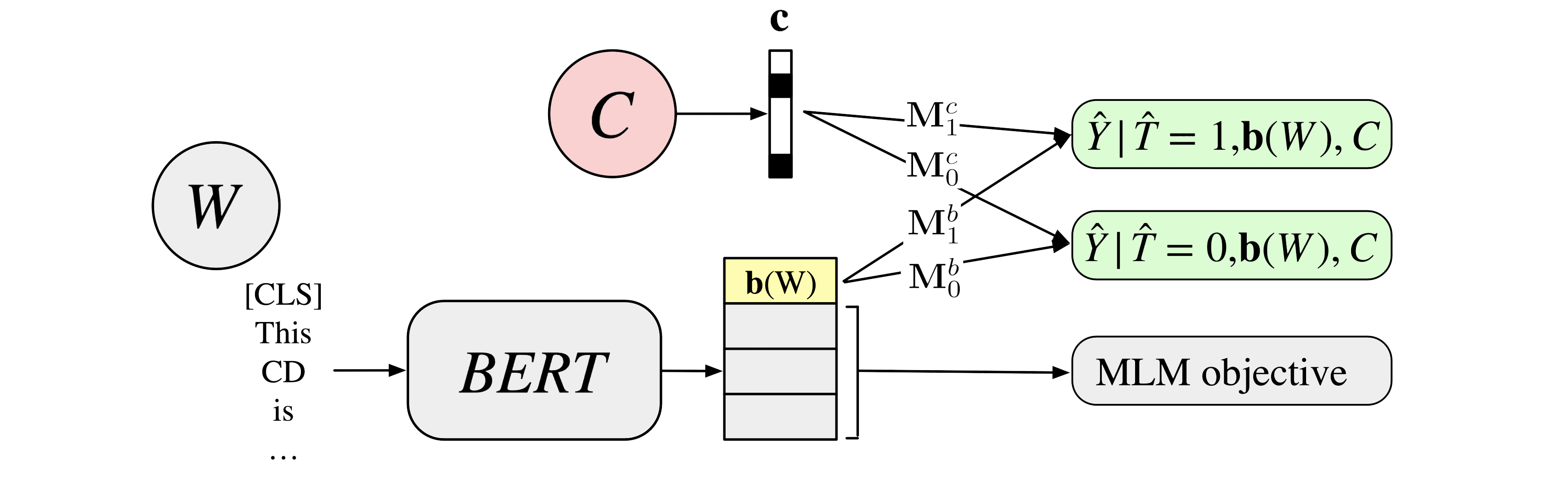
Figure 2: The second stage of TextCause adapts word embeddings to predict both of $Y$’s potential outcomes.

5 TextCause , A Causal Estimation Procedure

We introduce a practical algorithm for estimating the causal effects of linguistic properties. Motivated by Theorem 2, we first describe an approach for improving the accuracy of proxy labels. We then use the improved proxy labels, text and outcomes to fit a model that extracts and adjusts for the confounding information in the text $\tilde{Z}$. In practice, one may observe additional covariates $C$ that capture confounding properties, e.g., the product that a review is about or complaint type. We will include these covariates in the estimation algorithm.

5.1 Improved Proxy Labels

The first stage of TextCause is motivated by Theorem 2, which said that a more accurate proxy can yield lower estimation bias. Accordingly, this stage uses distant supervision to improve the fidelity of lexicon-based proxy labels $\hat{T}$. In particular, we exploit an inductive bias of frequently used lexicon-based proxy treatments: the words in a lexicon correctly capture the linguistic property of interest (i.e., high precision, Tausczik and Pennebaker, 2010), but can omit words and discourse-level elements that also map to the desired property (i.e., low recall, Kim and Hovy, 2006; Rao and Ravichandran, 2009).

Motivated by work on lexicon induction and label propagation Hamilton et al. (2016); An et al. (2018), we improve the recall of proxy labels, training a classifier $P_{\theta}$ to predict the proxy label $\hat{T}$, then using that classifier to relabel examples which were labeled $\hat{T}=0$ but look like $\tilde{T}=1$. Formally, given a dataset of tuples $\{(Y_{i},W_{i},C_{i},\hat{T}_{i})\}_{i=1}^{n}$ the algorithm is:

1. Train a classifier to predict $P_{\theta}(\hat{T}\,|\,W)$, e.g., logistic regression trained with bag-of-words features and $\hat{T}$ labels.

2. Relabel some $\hat{T}=0$ examples (we experiment with ablating this in Appendix C):
   $\hat{T}^{*}_{i}=\begin{cases}1&\text{if }\hat{T}_{i}=1\\ \mathbbm{1}[{P}_{\theta}(\hat{T}_{i}=1|W_{i})>0.5]&\text{otherwise}\end{cases}$

3. Use $\hat{T}^{*}$ as the new proxy treatment variable.

5.2 Adjusting for Text

The second stage of TextCause estimates the effect $\psi^{\textrm{proxy}}$ using the text $W$, improved proxy labels $\hat{T}^{*}$, and outcomes $Y$. This stage is motivated by Theorem 1, which described how to adjust for the confounding parts of the text. We approximate this confounding information in the text, $\tilde{Z}=f(W)$, with a learned representation $\mathbf{b}(W)$ that predicts the expected outcomes $\mathbb{E}[Y\,|\,\hat{T}^{*}=t,\mathbf{b}(W),C]$ for $t=0,1$ (Eq. 7).

We use DistilBERT Sanh et al. (2019) to produce a representation of the text $\mathbf{b}(W)$ by embedding the text then selecting the vector corresponding to a prepended [CLS] token. We proceed to optimize the model so that the representation $\mathbf{b}(W)$ directly approximates the confounding information $\tilde{Z}=f(w)$. In particular, we train an estimator for the expected conditional outcome $Q(t,\mathbf{b}(W),C)=\mathbb{E}[Y\,|\,\hat{T}^{*}=t,\mathbf{b}(W),C]$:

$$\hat{Q}(t,\mathbf{b}(W),C) =\sigma(\mathbf{M}^{b}_{t}\mathbf{b}(W)+\mathbf{M}^{c}_{t}\mathbf{c}+b)),$$

where the vector $\mathbf{c}$ is a one-hot encoding of the covariates $C$, the vectors $\mathbf{M}^{b}_{t}\in\mathbb{R}^{768}$ and $\mathbf{M}^{c}_{t}\in\mathbb{R}^{|C|}$ are learned, one for each value $t$ of the treatment, and the scalar $b$ is a bias term.

Letting $\theta$ be all parameters of the model, our training objective is to minimize,

$$\min_{\theta}\sum_{i=1}^{n}L(Y_{i},\hat{Q}_{\theta}(\hat{T}^{*}_{i},\mathbf{b}(W_{i}),C_{i}))+\alpha\cdot R(W_{i}),$$

where $L(\cdot)$ is the cross-entropy loss and $R(\cdot)$ is the original BERT masked language modeling objective, which we include following Veitch et al. (2020). The hyperparameter $\alpha$ is a penalty for the masked language modeling objective. The parameters $\mathbf{M}_{t}$ are updated on examples where $\hat{T}^{*}_{i}=t$.

Once $\hat{Q}(\cdot)$ is fitted, an estimator $\hat{\psi}^{\textrm{proxy}}$ for the effect $\psi^{\textrm{proxy}}$ (Eq. 7) is,

$$\hat{\psi}^{\textrm{proxy}}= \frac{1}{n}\sum_{i}\Big{[}\hat{Q}(1,\mathbf{b}(W_{i}),C_{i})$$

$$\quad\quad\quad\quad-\hat{Q}(0,\mathbf{b}(W_{i}),C_{i})\Big{]},$$ (9)

where we approximate the outer expectation over the text $W$ with a sample average. Intuitively, this procedure works because the representation $\mathbf{b}(W)$ extracts the confounding information $\tilde{Z}=f(W)$; it explains the outcome $Y$ as well as possible given the proxy label $\hat{T}^{*}$.

6 Experiments

We evaluate the proposed algorithm’s ability to recover causal effects of linguistic properties. Since ground-truth causal effects are unavailable without randomized controlled trials, we produce a semi-synthetic dataset based on Amazon reviews where only the outcomes are simulated. We also conduct an applied study using real-world complaints and bureaucratic response times. Our key findings are

• More accurate proxies combined with text adjustment leads to more accurate ATE estimates.

• Naive proxy-based procedures significantly underestimate true causal effects.

• ATE estimates can lose fidelity when the proxy is less than 80% accurate.

6.1 Amazon Reviews

6.1.1 Experimental Setup

Dataset. Here we use real world and publicly available Amazon review data to answer the question, “how much does a positive product review affect sales?” We create a scenario where positive reviews increase sales, but this effect is confounded by the type of product. Specifically:

• The text $W$ is a publicly available corpus of Amazon reviews for digital music products Ni et al. (2019). For simplicity, we only include reviews for mp3, CD, or Vinyl. We also exclude reviews for products worth more than $100 or fewer than 5 words.

• The observed covariate $C$ is a binary indicator for whether the associated review is a CD or not, and we use this to simulate a confounded outcome.

• The treatment $T=\tilde{T}$ is whether that review is positive (5 stars) or not (1 or 2 stars). Hence, we omit reviews with 3 or 4 stars. Note that here it is reasonable to assume writer’s intention ($T$) equals the reader’s perception ($\tilde{T}$), as the author is deliberately communicating their sentiment (or a very close proxy) with the stars. We use this variable to (1) simulate outcomes and (2) calculate ground truth causal effects for evaluation.

• The proxy treatment $\hat{T}$ is computed via two strategies: (1) a randomly noised version of $T$ fixed to 93% accuracy (to resemble a reasonable classifier’s output, later called “proxy-noised”), and (2) a binary indicator for whether any words in $W$ overlap with a positive sentiment lexicon Liu et al. (2010).

• The outcome $Y\sim\mathrm{Bernoulli}(\sigma(\beta_{c}(\pi(C)-\beta_{o})+\beta_{t}\tilde{T}+\mathbb{N}(0,\gamma)))$ represents whether a product received a click or not. The parameter $\beta_{c}$ controls confound strength, $\beta_{t}$ controls treatment strength, $\beta_{o}$ is an offset and the propensity $\pi(C)=P(T=1|C)$ is estimated from data.

The final data set consists of 17,000 examples.

Protocol. All nonlinear models were implemented using PyTorch Paszke et al. (2019). We use the transformers implementation of DistillBERT and the distilbert-base-uncased model, which has 66M parameters. To this we added 3,080 parameters for text adjustment (the $\mathbf{M^{b}_{t}}$ and $\mathbf{M^{c}_{t}}$ vectors). Models were trained in a cross-validated fashion, with the data being split into 12,000, 2,000, and 4,000-example train, validation, and test sets. BERT was optimized for 3 epochs on each fold using Adam Kingma and Ba (2014), a learning rate of $2e^{-5}$, and a batch size of 32. The weighting on the potential outcome and masked language modeling heads was 0.1 and 1.0, respectively. Linear models were implemented with sklearn. For T-boosting, we used a vocab size of 2,000 and L2 regularization with a strength of $c=1e^{-4}$. Each experiment was replicated using 100 different random seeds for robustness. Each trial took an average of 32 minutes with three 1.2 GHz CPU cores and one TITAN X GPU.

Baselines. The “unadjusted” baseline is $\hat{\psi}^{\textrm{naive}}=\hat{\operatorname{\mathbb{E}}}[Y|\hat{T}=1]-\hat{\operatorname{\mathbb{E}}}[Y|\hat{T}=0]$, the expected difference in outcomes conditioned on $\hat{T}$. The proxy-* baselines perform backdoor adjustment for the observed covariate $C$ and are based on Sridhar and Getoor (2019): $\hat{\psi}^{\textrm{naive+C}}=\frac{1}{|C|}\sum_{c}(\hat{\operatorname{\mathbb{E}}}[Y|\hat{T}=1,C=c]-\hat{\operatorname{\mathbb{E}}}[Y|\hat{T}=0,C=c])$, using randomly drawn and lexicon-based $\hat{T}$ proxies. We also compare against “semi-oracle”, $\hat{\psi}^{matrix}$, an estimator which assumes additional access to the ground truth measurement model $P(\hat{T}\,|\,T)$ Wood-Doughty et al. (2018); see Appendix G for derivation.

Note that for clarity, we henceforth refer to the treatment-boosting and text-adjusting stages of TextCause as T-boost and W-Adjust .

6.1.2 Results

Our primary results are summarized in Table 1. Individually, T-boost and W-Adjust perform well, generating estimates which are closer to the oracle than the naive “unadjusted” and “proxy-lex’ baselines. However, these components fail to outperform the highly accurate “proxy-noised” baseline unless they are combined (i.e., the TextCause algorithm). Only the full ${\sc TextCause}$ algorithm consistently outperformed (i.e. produced higher quality ATE estimates) than the baselines. This result is robust to varying levels of noise and treatment/confound strength. Indeed TextCause ’s estimates were on average within 2% of the semi-oracle. Furthermore, these results support Theorem 2: methods which adjusted for the text always attenuated the true ATE.

Noise:	Low				High
Treatment:	Low		High		Low		High		Mean delta
Confounding:	Low	High	Low	High	Low	High	Low	High	from oracle
oracle ($\psi$)	9.92	10.03	18.98	19.30	8.28	8.28	16.04	16.19	0.0
semi-oracle ($\hat{\psi}^{matrix}$)	9.73	9.82	18.77	19.08	8.25	8.28	16.02	16.21	0.13
unadjusted ($\hat{\psi}^{\textrm{naive}}$)	6.84	7.66	13.53	14.50	5.79	6.42	11.51	12.26	3.58
proxy-lex ($\hat{\psi}^{\textrm{naive+C}}$)	6.67	6.73	12.88	13.09	5.65	5.67	10.98	11.12	4.43
proxy-noised ($\hat{\psi}^{\textrm{naive+C}}$)	8.25	8.27	15.90	16.12	6.69	6.72	13.22	13.33	2.35
+T-boost ($\hat{\psi}^{\textrm{naive+C}}$)	8.11	8.16	15.53	15.73	6.78	6.80	13.19	13.32	2.51
+W-Adjust ($\hat{\psi}^{\textrm{proxy}}$)	7.82	8.57	14.96	16.13	6.62	7.22	12.95	13.76	2.39
+T-boost +W-Adjust	9.42	10.27	18.20	19.32	7.85	8.53	15.45	16.30	0.37
(TextCause , $\hat{\psi}^{\textrm{proxy}}$)

Table 1: ATE estimates: expected change in click probabilities if one were to manipulate the sentiment of a review from negative to positive. TextCause performs best in most settings. The true ATE is given in the top row (“oracle”). Estimates closer to the oracle are better. The last column gives the average difference between the estimated and true ATEs; lower is better. Rows 3-6 are baselines. Rows 7-9 are proposed. The second row and the bottom three rows use lexicon-based proxy treatments (we observed similar results using other proxy treatments). All columns have $\beta_{o}=0.9$. Low and high noise corresponds to $\gamma$ = 0 and 1. Low and high treatment corresponds to $\beta_{t}$ = 0.4, 0.8. Low and high confounding corresponds to $\beta_{c}$ = -0.4, 4.0. All standard errors are less than 0.5.

Our results suggest that adjusting for the confounding parts of text can be crucial: estimators that adjust for the covariates $C$ but not the text perform poorly, sometimes even worse than the unadjusted estimator $\hat{\psi}^{\textrm{naive}}$.

Does it always help to adjust for the text? We consider the case where confounding information in the text causes a naive estimator which does not adjust for this information ($\psi^{\textrm{naive}}$) to have the opposite sign of the true effect $\psi$. Does our proposed text adjustment help in this situation? Theorem 2 says it should, because $\psi^{\textrm{proxy}}$ estimates are bounded in [0, $\psi$]. This ensures that the most important of bits, the bit of directional information, is preserved.

Table 2 shows results from such a scenario. We see that the true ATE of $T$, $\psi$, has a strong negative effect, while the naive estimator $\psi^{\textrm{naive+C}}$ produces a positive effect. Adding an adjustment for the confounding parts of the text with TextCause successfully brings the proxy-based estimate to 0, which is indicative of the bounded behavior that Theorem 2 suggests.

Sensitivity analysis. In Figure 3 we synthetically vary the accuracy of a proxy $\hat{T}$ by dropping random subsets of the data. This is to evaluate the robustness of various estimation procedures. We would expect (1) methods that do not adjust for the text to behave unpredictably, and (2) methods that do adjust for the text to be more robust.

Estimator	ATE	SE
oracle ($\psi$)	-14.99	$\pm$ 0.1
proxy-lex ($\hat{\psi}^{\textrm{naive+C}}$)	6.29	$\pm$ 0.3
+T-boost ($\hat{\psi}^{\textrm{naive+C}}$)	4.18	$\pm$ 0.5
+T-boost +W-Adjust	0.50	$\pm$ 1.3
(TextCause , $\hat{\psi}^{\textrm{proxy}}$)

Table 2: Estimator performance in a worst-case scenario where the estimated ATE of $\hat{T}$ and $\hat{T}^{*}$ indicates the opposite sign of the true ATE of $T$ ($\beta_{c}=0.8$, $\beta_{t}=-1,\pi(C)=0.8$, $\beta_{o}=0.6$).

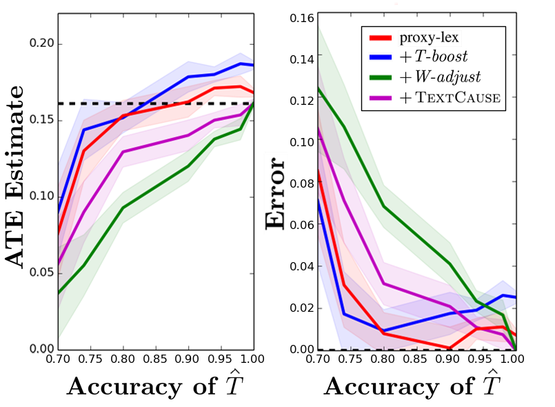
Figure 3: ATE estimates as the accuracy of $\hat{T}$ is varied. Without text adjustment, T-boost ’s errors can increase with the error rate of $\hat{T}$. The dotted black lines correspond to the true ATE (left) and 0 error (right).

These results support our first hypothesis: boosting treatment labels without text adjustment can behave unpredictably, as proxy-lex and T-boost both overestimate the true ATE. In other words, the predictions of both estimators grow further from the oracle as $\hat{T}$’s accuracy increases.

The results are mixed with respect to our second hypothesis. Both methods which adjust for the text (W-Adjust and TextCause ) consistently attenuate the true ATE, which is in line with Theorem 2. However, we find that TextCause , which makes use of T-boost and W-Adjust , may not always provide the highest quality ATE estimates in finite data regimes. Notably, when $\hat{T}$ is less than 90% accurate, both proxy-lex and T-boost can produce higher-quality estimates than the proposed TextCause algorithm.

Note that all estimates quickly lose fidelity as the proxy $\hat{T}$ becomes noisier. It rapidly becomes difficult for any method to recover the true ATE when the proxy $\hat{T}$ is less than 80% accurate.

6.2 Application: Complaints to the Financial Protection Bureau

We proceed to offer an applied pilot study which seeks to answer, “how does the perceived politeness of a complaint affect the time it takes for that complaint to be addressed?” We consider complaints filed with the Consumer Financial Protection Bureau (CFPB). This is a government agency which solicits and handles complaints about financial products. When they receive a complaint it is forwarded to the relevant company. The time it takes for that company to process the complaint is recorded. Some submissions are handled quickly ($<$ 15 days) while others languish. This 15-day threshold is our outcome $Y$. We additionally adjust for an observed covariate $C$ that captures what product and company the complaint is about (mortgage or bank account). To reduce other potentially confounding effects, we pair each $Y=1$ complaint with the most similar $Y=0$ complaint according to cosine similarity of TF-IDF vectors Mozer et al. (2020). From this we select the 4,000 most similar pairs for a total of 8,000 complaints.

For our treatment (politeness), we use a state-of-the-art politeness detection package geared towards social scientists Yeomans et al. (2018). This package reports a score from a trained classifier using expert features of politeness and a hand-labeled dataset. We take examples in the top and bottom 25% of the scoring distribution to be our $\hat{T}=1$ and $\hat{T}=0$ examples and throw out all others. The final dataset consists of 4,000 complaints, topics, and outcomes.

We use the same training procedure and hyperparameters as Section 6.1, except now W-Adjust is trained for 9 epochs and each cross validation fold is of size 2,000.

Results are given in Figure 3 and suggest that perceived politeness may have an effect on reducing response time. We find that the effect size increases as we adjust for increasing amounts of information. The “unadjusted” approach which does not perform any adjustment produces the smallest ATE. “proxy-lex”, which only adjusts for covariates, indicated the second-smallest ATE. The W-Adjust and TextCause methods, which adjust for covariates and text, produced the largest ATE estimates. This suggests that there is a significant amount of confounding in real world studies, and the choice of estimator can yield highly varying conclusions.

Estimator	ATE	SE
unadjusted ($\hat{\psi}^{\textrm{naive}}$)	3.01	$\pm$ 0.3
proxy-lex ($\hat{\psi}^{\textrm{naive+C}}$)	4.03	$\pm$ 0.4
+T-boost ($\hat{\psi}^{\textrm{naive+C}}$)	9.64	$\pm$ 0.5
+W-Adjust ($\hat{\psi}^{\textrm{proxy}}$)	6.30	$\pm$ 1.6
+T-boost +W-Adjust	10.30	$\pm$ 2.1
TextCause , ($\hat{\psi}^{\textrm{proxy}}$ )

Table 3: Effect size can vary across estimation methods, with methods that adjust for more information producing larger ATEs. Each number represents the expected percent change in the likelihood of getting a timely response when the politeness of a complaint is hypothetically increased.

7 Related Work

Our focus fits into a body of work on text-based causal inference that includes text as treatments (Egami et al., 2018; Fong and Grimmer, 2016; Grimmer and Fong, 2020; Wood-Doughty et al., 2018), text as outcomes Egami et al. (2018), and text as confounders (Roberts et al. (2020); Veitch et al. (2020); see Keith et al. (2020) for a review of that space). We build on Veitch et al. (2020), which proposed a BERT-based text adjustment method similar to our W-Adjust algorithm. This paper is related to work by Grimmer and Fong (2020), which discusses assumptions needed to estimate causal effects of text-based treatments in randomized controlled trials. There is also work on discovering causal structure in text, as topics with latent variable models Fong and Grimmer (2016) and as words and n-grams with adversarial learning Pryzant et al. (2018b) and residualization Pryzant et al. (2018a). There is also a growing body of applications in the social sciences Hall (2017); Olteanu et al. (2017); Saha et al. (2019); Mozer et al. (2020); Karell and Freedman (2019); Sobolev (2019); Zhang et al. (2020).

This paper also fits into a long-standing body of work on measurement error and causal inference (Pearl, 2012; Kuroki and Pearl, 2014; Buonaccorsi, 2010; Carroll et al., 2006; Shu and Yi, 2019; Oktay et al., 2019; Wood-Doughty et al., 2018). Most of this work deals with proxies for confounding variables. The present paper is most closely related to Wood-Doughty et al. (2018), which also deals with proxy treatments, but instead proposes an adjustment using the measurement model.

8 Conclusion

This paper addressed a setting of interest to NLP and social science researchers: estimating the causal effects of latent linguistic properties from observational data. We clarified critical ambiguities in the problem, showed how causal effects can be interpreted, presented a method, and demonstrated how it offers practical and theoretical advantages over the existing practice. We also release a package for performing text-based causal inferences. This work opens new avenues for further conceptual, methodological, and theoretical refinement. This includes improving non-lexicon based treatments, heterogeneous effects, overlap violations, counterfactual inference, ethical considerations, extensions to higher-dimensional outcomes and covariates, and benchmark datasets based on paired randomized controlled trials and observational studies.

9 Acknowledgements

This project recieved partial funding from the Stanford Data Science Institute, NSF Award IIS-1514268 and a Google Faculty Research Award. We thank Justin Grimmer, Stefan Wager, Percy Liang, Tatsunori Hashimoto, Zach Wood-Doughty, Katherine Keith, the Stanford NLP Group, and our anonymous reviewers for their thoughtful comments and suggestions.

Appendix A Proof of Theorem 1

Consider the expected outcome $\mu(t)=\mathbb{E}\left[Y\,;\,\mathrm{do}(\tilde{T}=t)\right]$.

$$\mu(t) =\mathbb{E}_{W}\bigg{[}\mathbb{E}\left[Y\,|\,W\,;\,\mathrm{do}(\tilde{T}=t)\right]\bigg{]}$$ (10)

(by iterated expectation)

$$=\mathbb{E}_{W}\bigg{[}\mathbb{E}\left[Y\,|\,\tilde{T},\tilde{Z}\,;\,\mathrm{do}(\tilde{T}=t)\right]\bigg{]}$$ (11)

(by definition)

$$=\mathbb{E}_{W}\bigg{[}\mathbb{E}\left[Y\,|\,\tilde{T}=t,\tilde{Z}\right]\bigg{]}$$ (12)

(by overlap and no unobserved confounding)

The proof is complete because the estimand $\psi^{\textrm{rea.}}$ is simply $\mu(1)-\mu(0)$.

Appendix B $C$-restriction

Section 4 said that adjusting for confounding information $\tilde{Z}=f(W)$ is sufficient for blocking the confounding backdoor path created by non-treatment properties of the text that readers might perceive. In Section 5.2 we proposed performing this adjustment with BERT. We could alternatively try to block this path by restricting a $\hat{T}$-boosting model to only use information related to the confounding covariates $C$ (for which we can adjust). This could capture the same desired effect as conditioning on $\tilde{Z}=f(W)$ by accounting for whatever extra information was leaked from $W$ into $\hat{T}$. We accordingly experiment with restricting the model to features that are highly correlated with $C$: we compute point-biserial correlation coefficients Glass and Hopkins (1996) between each word and $C$, then select the top 2000 words as features for the bootstrapping model. Results are given in Table 4 and suggest that while it still gives an improvement over the raw $\hat{T}$’s, $C$-restriction yields more conservative estimates than adjusting for $W$.

	Lexicon	BERT	Random
oracle ($\psi$)	15.54	15.54	15.54
proxy-lex ($\hat{\psi}^{\textrm{naive+C}}$)	11.21	7.83	12.34
T-boost	13.30	10.92	12.70
(C only, $\hat{\psi}^{\textrm{naive+C}}$)
T-boost ($\hat{\psi}^{\textrm{naive+C}}$)	14.68	12.01	13.59
W-Adjust ($\psi^{\textrm{proxy}}$)	15.01	13.88	13.30

Table 4: ATE estimates from a $C$-restricted classifier (row 2) are preferable to $\hat{T}$ but conservative compared to less restrictive methods (T-boost and W-Adjust ).

Appendix C Ablating T-boost

T-boost only uses a classifier to change the treatment status of an example on $\hat{T}=0$ examples. Intuitively, this is because $\hat{T}$ is assumed to be a reasonable estimate of $\tilde{T}$ and therefore has a low false positive rate. We investigate this by ablating this part of the algorithm and directly setting $\hat{T}^{*}$ to the classifier’s prediction. Our results on lexicon-based $\hat{T}$’s (Table 5, we observed similar outcomes with other $\hat{T}$’s) suggest this can reduce performance because a large number of correctly labeled $\hat{T}=1$ examples are flipped.

Estimator	Estimate
oracle ($\psi$)	15.54
proxy-lex ($\hat{\psi}^{\textrm{naive+C}}$)	11.21
T-boost ($\hat{T}=0$ only, $\hat{\psi}^{\textrm{naive+C}}$)	14.60
T-boost (all examples, $\hat{\psi}^{\textrm{naive+C}}$)	10.00

Table 5: It is advantageous to only relabel $\hat{T}=0$ examples.

Appendix D Lemma 1 (used by Theorems 2 and 3)

$$\operatorname{\mathbb{E}}[Y\mid W,\hat{T}=1] =\operatorname{\mathbb{E}}[Y\mid W,T=1]\Pr(T=1\mid W,\hat{T}=1)$$

$$+\operatorname{\mathbb{E}}[Y\mid W,T=0]\Pr(T=0\mid W,\hat{T}=1)$$

$$\operatorname{\mathbb{E}}[Y\mid W,\hat{T}=0] =\operatorname{\mathbb{E}}[Y\mid W,T=0]\Pr(T=0\mid W,\hat{T}=0)$$

$$+\operatorname{\mathbb{E}}[Y\mid W,T=1]\Pr(T=1\mid W,\hat{T}=0)$$

Proof.

Apply the law of total probability and definition of conditional independence to the causal graph given in Figure 3. ∎

Appendix E Proof of Theorem 2

Let

$$\epsilon_{0} =P(T=0\,|\,\hat{T}=1,\tilde{Z})$$

$$\epsilon_{1} =P(T=1\,|\,\hat{T}=0,\tilde{Z},C)$$

$$p_{1} =P(T=1\,|\,\hat{T}=1,\tilde{Z})$$

$$p_{0} =P(T=0\,|\,\hat{T}=0,\tilde{Z})$$

$$E_{1} =\mathbb{E}[Y\,|\,\tilde{Z},T=1]$$

$$E_{0} =\mathbb{E}[Y\,|\,\tilde{Z},T=0]$$

Now recall

$$\hat{\psi}^{\textrm{proxy}} =\operatorname{\mathbb{E}}_{W}[\operatorname{\mathbb{E}}[Y\,|\,\hat{T}=1,\tilde{Z}]-\operatorname{\mathbb{E}}[Y\,|\,\hat{T}=0,\tilde{Z}]]$$

Now we write the inner part using Lemma D, collect terms, and use the law of total probability to write everything in terms of misclassification probabilities:

$$=(E_{1}p_{1}+E_{0}\epsilon_{0})-(E_{0}p_{0}-E_{1}\epsilon_{1})$$

$$=E_{1}(p_{1}+\epsilon_{1})+E_{0}(\epsilon_{0}-p_{0})$$

$$=E_{1}((1-\epsilon_{0})+\epsilon_{1})+E_{0}(\epsilon_{0}-(1-\epsilon_{1}))$$

$$=(E_{1}-E_{0})(1-(\epsilon_{0}+\epsilon_{1}))$$

which completes the proof $\square$

Appendix F Theorem about the bias due to noisy proxies

Here we show that the naive estimand which does not adjust for the text,

$$\psi^{\textrm{naive}}=\mathbb{E}\left[Y\,|\,\hat{T}=1\right]-\mathbb{E}\left[Y\,|\,\hat{T}=0\right],$$ (13)

can be arbitrarily biased away from the effect of interest, $\psi^{\textrm{rea.}}$.

Theorem 3.

$$\psi^{\textrm{naive}}=\mathbb{E}_{W}\big{[}\operatorname{\mathbb{E}}[Y\,|\,\tilde{T}=1,W]\alpha(W)\ -\ \operatorname{\mathbb{E}}[Y\,|\,\tilde{T}=0,W]\beta(W)\big{]}$$

where

$$\alpha(W) =\frac{P(\tilde{T}=1,\hat{T}=1\,|\,W)}{P(\hat{T}=1)}-\frac{P(\tilde{T}=1,\hat{T}=0\,|\,W)}{P(\hat{T}=0)}$$

$$\beta(W) =\frac{P(\tilde{T}=0,\hat{T}=0\,|\,W)}{P(\hat{T}=0)}-\frac{P(\tilde{T}=0,\hat{T}=1\,|\,W)}{P(\hat{T}=1)}$$

The $\alpha$ and $\beta$ terms are related to the error of the proxy label. This theorem says that correlations between the outcome and errors in the proxy can induce bias. Intuitively, this is similar to bias from confounding, though it is mathematically distinct. This means that even a highly accurate proxy label can result in highly misleading estimates. Proof:

$$\operatorname{\mathbb{E}}[Y\mid\hat{T}=1] =\operatorname{\mathbb{E}}\big{[}\operatorname{\mathbb{E}}[Y\mid\hat{T}=1,W]\mid\hat{T}=1\big{]}$$

$$=\operatorname{\mathbb{E}}\left[\operatorname{\mathbb{E}}[Y\mid\hat{T}=1,W]\frac{\Pr(W\mid\hat{T}=1)}{\Pr(W)}\right]$$

$$=\operatorname{\mathbb{E}}\left[\operatorname{\mathbb{E}}[Y\mid\hat{T}=1,W]\frac{\Pr(\hat{T}=1\mid W)}{\Pr(\hat{T}=1)}\right]$$

Where the first equality is by the tower property, the second by inverse probability weighting, and the third Bayes’ rule. We continue by invoking Lemma 1:

$$\operatorname{\mathbb{E}}[Y\mid\hat{T}=1,W]\frac{\Pr(\hat{T}=1\mid W)}{\Pr(\hat{T}=1)} =\operatorname{\mathbb{E}}[Y\mid W,T=1]\Pr(T=1\mid W,\hat{T}=1)\frac{\Pr(\hat{T}=1\mid W)}{\Pr(\hat{T}=1)}$$

$$\quad\quad+\operatorname{\mathbb{E}}[Y\mid W,T=0]\Pr(T=0\mid W,\hat{T}=1)\frac{\Pr(\hat{T}=1\mid W)}{\Pr(\hat{T}=1)}$$

$$=\operatorname{\mathbb{E}}[Y\mid W,T=1]\frac{\Pr(T=1,\hat{T}=1\mid W)}{\Pr(\hat{T}=1)}$$

$$\quad\quad+\operatorname{\mathbb{E}}[Y\mid W,T=0]\frac{\Pr(T=0,\hat{T}=1\mid W)}{\Pr(\hat{T}=1)}.$$

The analogous expression for $\operatorname{\mathbb{E}}[Y\mid\hat{T}=0]$:

$$\operatorname{\mathbb{E}}[Y\mid\hat{T}=0] =\operatorname{\mathbb{E}}\Bigg{[}\operatorname{\mathbb{E}}[Y\mid W,T=0]\frac{\Pr(T=0,\hat{T}=0\mid W)}{\Pr(\hat{T}=0)}$$

$$\quad\quad\quad+\operatorname{\mathbb{E}}[Y\mid W,T=1]\frac{\Pr(T=1,\hat{T}=0\mid W)}{\Pr(\hat{T}=0)}\Bigg{]}$$

And now plugging into the ATE formula:

$$\hat{\psi}^{\textrm{rea.}}=\operatorname{\mathbb{E}}[\operatorname{\mathbb{E}}[Y;do(\hat{T}=1)]-\operatorname{\mathbb{E}}[Y;do(\hat{T}=0)]]$$

$$\quad\ =\operatorname{\mathbb{E}}[\operatorname{\mathbb{E}}[Y|\hat{T}=1]-\operatorname{\mathbb{E}}[Y|\hat{T}=0]]$$

$$\quad\ =\operatorname{\mathbb{E}}\Big{[}$$

$$\quad\quad\quad\operatorname{\mathbb{E}}[Y\mid W,T=1]\Big{(}\frac{\Pr(T=1,\hat{T}=1\mid W)}{\Pr(\hat{T}=1)}-\frac{\Pr(T=1,\hat{T}=0\mid W)}{\Pr(\hat{T}=0)}\Big{)}$$

$$\quad\quad\quad-\operatorname{\mathbb{E}}[Y\mid W,T=0]\Big{(}\frac{\Pr(T=0,\hat{T}=0\mid W)}{\Pr(\hat{T}=0)}-\frac{\Pr(T=0,\hat{T}=1\mid W)}{\Pr(\hat{T}=1)}\Big{)}$$

$$\quad\quad\quad\ \Big{]}$$

The result follows immediately. $\square$

Appendix G Deriving semi-oracle, a Causal Estimator for when $P(T|\hat{T})$ is known

This is an ATE estimator which assumes access to $P(\hat{T}|T)$ instead of $T$ but is still unbiased. We derive this estimator using the “matrix adjustment” technique of Wood-Doughty et al. (2018); Pearl(2012). We start by decomposing the joint distribution

$$P(Y,T,\hat{T},C) =P(\hat{T}|Y,C,T)P(Y,C,T)$$

$$P(Y,C,\hat{T}) =\sum_{T}P(\hat{T}|Y,C,T)P(Y,C,T)$$

We can write this as a product between a matrix $\mathbf{M}_{c,y}(\hat{T},T)=P(\hat{T}|Y,C,T)$ and vector $\mathbf{V}_{c,y}(T)=P(Y,C,T)$:

$$\mathbf{V}_{c,y}(\hat{T}) =\sum_{T}\mathbf{M}_{c,y}(\hat{T},T)\mathbf{V}_{c,y}(T)$$

$$=\mathbf{M}_{c,y}\mathbf{V}_{c,y}$$

For our binary setting $\mathbf{M}_{c,y}$ is:

$$\mathbf{M}_{c,y} =\begin{bmatrix}1-\delta_{c,y}&\epsilon_{c,y}\\ \delta_{c,y}&1-\epsilon_{c,y}\end{bmatrix}$$

$$\mathbf{M}_{c,y}^{-1} =\frac{1}{1-\epsilon_{c,y}-\delta_{c,y}}\begin{bmatrix}1-\epsilon_{c,y}&-\epsilon_{c,y}\\ -\delta_{c,y}&1-\delta_{c,y}\end{bmatrix}$$

$$\epsilon_{c,y} =P(\hat{T}=0|T=1,C,Y)$$

$$\delta_{c,y} =P(\hat{T}=1|T=0,C,Y)$$

Under fairly broad conditions, $\mathbf{M}$ has an inverse, which allows us to reconstruct the joint distribution:

$$P(Y,T,C)=\sum_{\hat{T}}\mathbf{M}^{-1}_{c,y}(T,\hat{T})\mathbf{V}_{c,y}(\hat{T})$$

From which we can recover the ATE

$$\psi^{matrix} =\sum_{c}\left[\frac{P(Y,T=1,C)}{\sum_{Y}P(Y,T=1,C)}-\frac{P(Y,T=0,C)}{\sum_{Y}P(Y,T=0,C)}\right]\ P(C)$$

Note also that this expression is similar to $\tau_{ME}$ in Wood-Doughty et al. (2018) except their error terms are of the form $P(T\,|\,\hat{T})$.

References

- An et al. (2018) Jisun An, Haewoon Kwak, and Yong-Yeol Ahn. 2018. Semaxis: A lightweight framework to characterize domain-specific word semantics beyond sentiment. In Proceedings of ACL.
- Buonaccorsi (2010) John P Buonaccorsi. 2010. Measurement error: models, methods, and applications. CRC press.
- Carroll et al. (2006) Raymond J Carroll, David Ruppert, Leonard A Stefanski, and Ciprian M Crainiceanu. 2006. Measurement error in nonlinear models: a modern perspective. CRC press.
- Devlin et al. (2018) Jacob Devlin, Ming-Wei Chang, Kenton Lee, and Kristina Toutanova. 2018. BERT: Pre-training of deep bidirectional transformers for language understanding. arXiv preprint arXiv:1810.04805.
- Egami et al. (2018) Naoki Egami, Christian J Fong, Justin Grimmer, Margaret E Roberts, and Brandon M Stewart. 2018. How to make causal inferences using texts. arXiv preprint arXiv:1802.02163.
- Fong and Grimmer (2016) Christian Fong and Justin Grimmer. 2016. Discovery of treatments from text corpora. In Proceedings of ACL, pages 1600–1609.
- Gibson et al. (2013) Edward Gibson, Leon Bergen, and Steven T Piantadosi. 2013. Rational integration of noisy evidence and prior semantic expectations in sentence interpretation. Proceedings of the National Academy of Sciences, 110(20):8051–8056.
- Glass and Hopkins (1996) Gene Glass and Kenneth Hopkins. 1996. Statistical methods in education and psychology. Psyccritiques, 41(12).
- Goodman and Frank (2016) Noah D Goodman and Michael C Frank. 2016. Pragmatic language interpretation as probabilistic inference. Trends in cognitive sciences, 20(11):818–829.
- Grimmer and Fong (2020) Justin Grimmer and Christian Fong. 2020. Causal inference with latent treatments. In Unpublished.
- Grimmer and Stewart (2013) Justin Grimmer and Brandon M Stewart. 2013. Text as data: The promise and pitfalls of automatic content analysis methods for political texts. Political analysis, 21(3):267–297.
- Hall (2017) Allie Hall. 2017. How hiring language reinforces pink collar jobs.
- Hamilton et al. (2016) William L Hamilton, Kevin Clark, Jure Leskovec, and Dan Jurafsky. 2016. Inducing domain-specific sentiment lexicons from unlabeled corpora. In Proceedings of EMNLP.
- Iser (1974) Wolfgang Iser. 1974. The implied reader: Patterns of communication in prose fiction from Bunyan to Beckett. Johns Hopkins University Press.
- Iser (1979) Wolfgang Iser. 1979. The act of reading: A theory of aesthetic response. Johns Hopkins University Press.
- Karell and Freedman (2019) Daniel Karell and Michael Freedman. 2019. Rhetorics of radicalism. American Sociological Review, 84(4):726–753.
- Keith et al. (2020) Katherine Keith, David Jenson, and Brendan O’Connor. 2020. Text and causal inference: A review of using text to remove confounding from causal estimates. In Proceedings of ACL.
- Kim and Hovy (2006) Soo-Min Kim and Eduard Hovy. 2006. Identifying and analyzing judgment opinions. In Proceedings of NAACL.
- Kingma and Ba (2014) Diederik P Kingma and Jimmy Ba. 2014. Adam: A method for stochastic optimization. In Proceedings of ICLR.
- Kuroki and Pearl (2014) Manabu Kuroki and Judea Pearl. 2014. Measurement bias and effect restoration in causal inference. Biometrika, 101(2):423–437.
- Levinson (1995) Stephen C. Levinson. 1995. Three levels of meaning. In Frank R. Palmer, editor, Grammar and Meaning: Essays in Honor of Sir John Lyons, pages 90–115. Cambridge University Press.
- Levinson (2000) Stephen C. Levinson. 2000. Presumptive Meanings: The Theory of Generalized Conversational Implicature. MIT Press, Cambridge, MA.
- Liu et al. (2010) Bing Liu et al. 2010. Sentiment analysis and subjectivity. Handbook of natural language processing, 2(2010):627–666.
- Lucas et al. (2015) Christopher Lucas, Richard A Nielsen, Margaret E Roberts, Brandon M Stewart, Alex Storer, and Dustin Tingley. 2015. Computer-assisted text analysis for comparative politics. Political Analysis, 23(2):254–277.
- Lucy et al. (2020) Li Lucy, Dorottya Demszky, Patricia Bromley, and Dan Jurafsky. 2020. Content analysis of textbooks via natural language processing: Findings on gender, race, and ethnicity in Texas U.S. history textbooks. AERA Open, 6(3).
- Luo et al. (2019) Yiwei Luo, Dan Jurafsky, and Beth Levin. 2019. From insanely jealous to insanely delicious: Computational models for the semantic bleaching of english intensifiers. In Proceedings of the 1st International Workshop on Computational Approaches to Historical Language Change.
- Mintz et al. (2009) Mike Mintz, Steven Bills, Rion Snow, and Dan Jurafsky. 2009. Distant supervision for relation extraction without labeled data. In Proceedings of ACL, pages 1003–1011.
- Mozer et al. (2020) Reagan Mozer, Luke Miratrix, Aaron Russell Kaufman, and L Jason Anastasopoulos. 2020. Matching with text data: An experimental evaluation of methods for matching documents and of measuring match quality. Political Analysis, 28(4):445–468.
- Ni et al. (2019) Jianmo Ni, Jiacheng Li, and Julian McAuley. 2019. Justifying recommendations using distantly-labeled reviews and fine-grained aspects. In Proceedings of EMNLP, pages 188–197.
- Oktay et al. (2019) Hüseyin Oktay, Akanksha Atrey, and David Jensen. 2019. Identifying when effect restoration will improve estimates of causal effect. In Proceedings of the 2019 SIAM International Conference on Data Mining, pages 190–198. SIAM.
- Olteanu et al. (2017) Alexandra Olteanu, Onur Varol, and Emre Kiciman. 2017. Distilling the outcomes of personal experiences: A propensity-scored analysis of social media. In Proceedings of CSCW.
- Paszke et al. (2019) Adam Paszke, Sam Gross, Francisco Massa, Adam Lerer, James Bradbury, Gregory Chanan, Trevor Killeen, Zeming Lin, Natalia Gimelshein, Luca Antiga, Alban Desmaison, Andreas Kopf, Edward Yang, Zachary DeVito, Martin Raison, Alykhan Tejani, Sasank Chilamkurthy, Benoit Steiner, Lu Fang, Junjie Bai, and Soumith Chintala. 2019. PyTorch: An imperative style, high-performance deep learning library. In Proceedings of NeurIPS.
- Pearl (2009) Judea Pearl. 2009. Causality. Cambridge university press.
- Pearl (2012) Judea Pearl. 2012. On measurement bias in causal inference. Proceedings of UAI.
- Potts (2009) Christopher Potts. 2009. Formal pragmatics. The Routledge Encyclopedia of Pragmatics.
- Prabhakaran et al. (2016) Vinodkumar Prabhakaran, William L Hamilton, Dan McFarland, and Dan Jurafsky. 2016. Predicting the rise and fall of scientific topics from trends in their rhetorical framing. In Proceedings of ACL, pages 1170–1180.
- Pryzant et al. (2018a) Reid Pryzant, Sugato Basu, and Kazoo Sone. 2018a. Interpretable neural architectures for attributing an ad’s performance to its writing style. In Proceedings of the 2018 EMNLP Workshop BlackboxNLP: Analyzing and Interpreting Neural Networks for NLP.
- Pryzant et al. (2017) Reid Pryzant, Youngjoo Chung, and Dan Jurafsky. 2017. Predicting sales from the language of product descriptions. In Proceedings of the SIGIR Workshop on eCommerce.
- Pryzant et al. (2018b) Reid Pryzant, Kelly Shen, Dan Jurafsky, and Stefan Wagner. 2018b. Deconfounded lexicon induction for interpretable social science. In Proceedings of NAACL, pages 1615–1625.
- Rao and Ravichandran (2009) Delip Rao and Deepak Ravichandran. 2009. Semi-supervised polarity lexicon induction. In Proceedings of EACL.
- Roberts et al. (2020) Margaret E Roberts, Brandon M Stewart, and Richard A Nielsen. 2020. Adjusting for confounding with text matching. American Journal of Political Science, 64(4):887–903.
- Rosenbaum and Rubin (1983) Paul R Rosenbaum and Donald B Rubin. 1983. The central role of the propensity score in observational studies for causal effects. Biometrika, 70(1):41–55.
- Rosenbaum and Rubin (1984) Paul R Rosenbaum and Donald B Rubin. 1984. Reducing bias in observational studies using subclassification on the propensity score. Journal of the American statistical Association, 79(387):516–524.
- Saha et al. (2019) Koustuv Saha, Benjamin Sugar, John Torous, Bruno Abrahao, Emre Kıcıman, and Munmun De Choudhury. 2019. A social media study on the effects of psychiatric medication use. In Proceedings of the International AAAI Conference on Web and Social Media.
- Sanh et al. (2019) Victor Sanh, Lysandre Debut, Julien Chaumond, and Thomas Wolf. 2019. DistilBERT, a distilled version of bert: smaller, faster, cheaper and lighter. arXiv preprint arXiv:1910.01108.
- Shalizi (2013) Cosma Shalizi. 2013. Advanced data analysis from an elementary point of view.
- Shu and Yi (2019) Di Shu and Grace Y Yi. 2019. Weighted causal inference methods with mismeasured covariates and misclassified outcomes. Statistics in medicine, 38(10):1835–1854.
- Sobolev (2019) Anton Sobolev. 2019. How pro-government “trolls” influence online conversations in russia. Unpublished.
- Sridhar and Getoor (2019) Dhanya Sridhar and Lise Getoor. 2019. Estimating causal effects of tone in online debates. Proceedings of IJCAI.
- Tausczik and Pennebaker (2010) Yla R Tausczik and James W Pennebaker. 2010. The psychological meaning of words: LIWC and computerized text analysis methods. Journal of language and social psychology, 29(1):24–54.
- Veitch et al. (2020) Victor Veitch, Dhanya Sridhar, and David Blei. 2020. Adapting text embeddings for causal inference. In Proceedings of UAI.
- Voigt et al. (2017) Rob Voigt, Nicholas P Camp, Vinodkumar Prabhakaran, William L Hamilton, Rebecca C Hetey, Camilla M Griffiths, David Jurgens, Dan Jurafsky, and Jennifer L Eberhardt. 2017. Language from police body camera footage shows racial disparities in officer respect. Proceedings of the National Academy of Sciences, 114(25):6521–6526.
- Wood-Doughty et al. (2018) Zach Wood-Doughty, Ilya Shpitser, and Mark Dredze. 2018. Challenges of using text classifiers for causal inference. In Proceedings of EMNLP.
- Yeomans et al. (2018) Michael Yeomans, Alejandro Kantor, and Dustin Tingley. 2018. The politeness package: Detecting politeness in natural language. R Journal, 10(2).
- Yuret and Yatbaz (2010) Deniz Yuret and Mehmet Ali Yatbaz. 2010. The noisy channel model for unsupervised word sense disambiguation. Computational Linguistics, 36(1):111–127.
- Zhang et al. (2020) Justine Zhang, Sendhil Mullainathan, and Cristian Danescu-Niculescu-Mizil. 2020. Quantifying the causal effects of conversational tendencies. Proceedings of CSCW.
- Zhur and Ghahramani (2002) Xiaojin Zhur and Zoubin Ghahramani. 2002. Learning from labeled and unlabeled data with label propagation. CMU CALD tech report.