Pointwise periodic maps with quantized first integrals

Abstract

We describe the global dynamics of some pointwise periodic piecewise linear maps in the plane that exhibit interesting dynamic features. For each of these maps we find a first integral. For these integrals the set of values are discrete, thus quantized. Furthermore, the level sets are bounded sets whose interior is formed by a finite number of open tiles of certain regular or uniform tessellations. The action of the maps on each invariant set of tiles is described geometrically.

Mathematics Subject Classification 2010: Primary: 37C25, 39A23. Secondary: 37C55, 37J35, 52C20.

Keywords: Periodic points; pointwise periodic maps; piecewise linear maps; quantized first integrals; regular and uniform tessellations.

1 Introduction

A pointwise periodic map is a bijective self-map in a topological space such that each point is periodic. A periodic map is a bijective self-map in a topological space such that some iterated of the map is the identity. For a periodic map $F:X\longrightarrow X$ the minimum natural number $p$ satisfying $F^{p}=\mathrm{Id}$ is called the period of $F.$ Notice that a pointwise periodic map satisfying that the period of the points has an upper bound is periodic and its period is the least common multiple of the periods of the elements of the space.

A classical result of Montgomery establishes that any pointwise periodic homeomeorphism in an Euclidean space is periodic, [19]. Non-periodic but pointwise periodic bijective maps do exist when the continuity assumption is relaxed, see [23] for instance. In the series of papers [7, 8] and [10], the authors introduce three explicit examples of pointwise periodic maps that are not periodic. The examples given by these authors in the above mentioned references belong to the family of piecewise affine maps with a line of discontinuity:

$$G(x,y)=\left(y,-x-\rho y+\operatorname{sign}(y)\right),\quad\mbox{where}\quad\operatorname{sign(y)}=\left\{\begin{array}[]{ll}+1,&\hbox{if $y\geq 0$;}\\ -1,&\hbox{otherwise,}\end{array}\right.$$ (1)

for $|\rho|<2.$ In particular they correspond to the cases $\rho\in\{-1,0,1\}$. There are other values of $\rho$ for which there exist non-periodic points, see [9]. Notice also that maps (1) correspond to the second order discontinuous difference equations $x_{n+2}=-x_{n}-\rho x_{n+1}+\operatorname{sign}(x_{n+1}).$

As we will see in next section, each map $G$ is linearly conjugate with the piecewise rotation map

$$F(x,y)=\left(\begin{array}[]{rr}\cos(\alpha)&\sin(\alpha)\\ -\sin(\alpha)&\cos(\alpha)\end{array}\right)\left(\begin{array}[]{ll}x-\operatorname{sign}(y)\\ y\end{array}\right),$$ (2)

where $\rho=-2\cos(\alpha)$ with $\alpha\in(0,\pi).$ Observe that the maps $G$ with $\rho=-1,0$ and $1$ are conjugate with the maps $F$ with $\alpha={\pi}/{3},{\pi}/{2}$ and ${2\pi}/{3},$ respectively. As we will see, the normal form $F$ regularizes the shape of the invariant sets and keeps the same discontinuity line $y=0.$ These maps are included in the class of symmetric maps studied in the remarkable paper [14] together with other more general piecewise rotations, see a further comment below. As noticed in [5], they exhibit complex dynamics and they belong to the type of piecewise rotations with the same rotation angle that elude the generic dichotomy that appears in most piecewise rotations of being globally attracting or globally repelling maps, see [5, Theorem 1].

Piecewise affine maps with a line of discontinuity appear as models in many fields like in the study of mechanical systems with friction, power electronics, relay control systems or economics [2, 6, 24]. In fact, as is explained in [7, 8, 10], the three maps (1) with $\rho\in\{-1,0,1\}$ appear in the study of steady states of certain cellular neural networks. Despite their apparent simplicity, piecewise affine maps exhibit great dynamic richness and a variety of phenomena that are characteristic of these systems, see [3, 5, 14, 22, 24] and references therein. As we will show, the examples considered in this paper are also very rich from a dynamical viewpoint, even though each orbit is periodic. In fact, one of our motivations was to highlight the beautiful features of these examples.

Recall that a first integral of a discrete dynamical system associated with a map $F$ is a non-constant real valuated function $V$ such that $V\circ F=V$, which means that the level sets $\{V=c\}$, typically called the energy levels, are invariant under the action of the map. It is known that periodicity issues are related with integrability since most continuous periodic maps are completely integrable (there exist as many functionally independent first integrals as the dimension of the phase space), see [11] and [12]. In this work we consider the piecewise affine maps $F$ with $\alpha\in\{\pi/3,\pi/2,2\pi/3\}$ under the light of their properties as integrable systems. For each of these three maps, we obtain a non-trivial first integral which is defined in an open and dense set of ${\mathbb{R}}^{2}$ and have discrete (or quantized) energy levels. Then we describe their global features in terms of the dynamics induced by the maps on the level sets of the first integrals. These level sets are bounded, with positive measure and their interior is formed by a finite number of some prescribed tiles of certain regular or uniform tessellations forming necklaces, see Figures 1, 2 and 3. The existence of necklaces in piecewise isometries is well known. For instance, in [14, Theorem 1 and Lemma 11] it is established the existence of some invariant necklaces defined by convex polygons containing periodic islands for a family of maps that contain the ones studied in this papers. These necklaces and the set of periods associated with their periodic orbits are characterized both analytically and geometrically, and its existence is the key to prove the boundedness of the orbits of the maps considered there. We want to point out that in our maps, all the integral’s level sets are necklaces. In Remark 2 we comment the relation between both families of necklaces. In addition, as we will see, the maps $F$ with $\alpha\in\{\pi/3,\pi/2,2\pi/3\}$ have also a second continuous first integral, see Remark 23. This second first integral, however, is not useful to control the set of periods.

Planar piecewise isometries appear in the study of polygonal dual billiards ([13, 17, 20]). The results in the literature indicate that some polygonal dual billiards should also have quantized integrals, see Figure 3 in [20], Figure 2 in [13], or Figures 3–5 and the results in [23]. We believe that the explicitness of the analytic expression of the quantized integrals with positive measure level sets for the maps (2) is quite novel in the context of discrete dynamical systems theory. It is interesting to notice the fact that the regular tessellations that we find in this paper also appear in the study of some polygonal dual billiards like the one introduced by Moser in [20] or those that appear in [23]. Observe, however, that these dual billiards are not conjugated to any map considered in our paper, because they exhibit different sets of periods.

A consequence of our results for $F,$ when $\alpha\in\{\pi/3,\pi/2,2\pi/3\},$ is the existence of an open and dense subset $\mathcal{U}$ on which the dynamics of the map is strongly stable and simple. We will see that for any $x\in\mathcal{U}$ there exists an open neighborhood of $x$, say $\mathcal{U}_{x}$, and $n_{x}\in{\mathbb{N}}$ such that $F^{n_{x}}|_{\mathcal{U}_{x}}=\operatorname{Id}.$ Moreover, varying $x\in\mathcal{U},$ the values $n_{x}$ are unbounded.

We will study the three cases separately in three different sections. In a few words, the main results that we will state in detail in the next section, are:

1. We present first integrals $V$ for each case. See Section 6 for a constructive approach for obtaining them.

2. The interior of the level sets of each first integral is described in terms of some prescribed open tiles of a regular or uniform tessellation of ${\mathbb{R}}^{2}$, see Figures 1, 2 and 3. In all cases, each of them is a necklace whose beads (the open tiles) are open sets having one of the following three shapes: squares ($\alpha=\pi/2),$ triangles and hexagons ($\alpha\in\{\pi/3,2\pi/3\}$). In the three figures the beads of a necklace have the same color. In fact, the shape and the number of beads, say $M,$ only depend on the level set $k$ and $\alpha.$ Moreover, the inter-tile dynamics can be described in a very simple way: if we collapse each of the open tiles in a point, the interior of $\{(x,y):V(x,y)=c\}$ can be identified with ${\mathbb{Z}}_{M},$ simply following the order given by the necklace in clockwise sense, were, as usual, given $q\in{\mathbb{Z}},$ we denote by ${\mathbb{Z}}_{q}$ the set of the residue classes induced by the congruence $n\equiv m$ if and only if $n-m$ is a multiple of $q$ with $n,m\in{\mathbb{Z}}$. Then we will prove that the dynamical system generated by $F,$ restricted to this set, is conjugated to an affine discrete dynamical system generated by a map $h:{\mathbb{Z}}_{M}\to{\mathbb{Z}}_{M}$, where $h(i)=i+u(c,\alpha),$ for some $u(c,\alpha)\in{\mathbb{Z}}_{M}$ that we also determine explicitly in this paper, see Theorems A, B and C. Notice that, geometrically, $F$ acts as a rotation among the beads of any necklace. A similar inter-tile dynamics’ description in the context of dual polygonal billiards can be found in [17], and also in the context of piecewise linear maps [14, Theorem 1 and Lemma 11].

   Due to the above conjugation, the dynamics on the interior of each level set can be completely understood, see Theorems A, B and C. Roughly speaking, for each map and for each necklace (set of tiles with the same energy level), there exists a certain number $k\in\{M,M/2\}\cap{\mathbb{N}}$, that depends (explicitly) on the energy level, so that each tile is invariant by $F^{k}$. Furthermore, on each tile, $F^{k}$ is a rotation of order $p$ around the center of the tile, where $p\in\{2,4\}$ when $\alpha=\pi/2$, or $p\in\{3,6\}$ when $\alpha\in\{\pi/3,2\pi/3\}$ and it is determined explicitly by the energy level. As a consequence, on each tile there is a $k$-periodic point (the center) and the rest of points are $kp$-periodic. The dynamics in the necklaces is, therefore, a discrete version of an epicyclic motion around a discrete deferent which is the locus of the centers of the tiles, [21, p. 123].

   As we will see, the dynamics on the boundaries of the tiles (edges and vertices) requires a little bit more elaborated description.

3. As a consequence of the above results and the study of the dynamics on the boundary of the level sets, for each map, we easily characterize the period of every point in terms of the value of its associate first integral and obtain the global dynamics of the map. For instance in Proposition 1 we present our results in an algorithmic way when $\alpha=\pi/2.$ In particular, the set of periods of the maps are presented.

2 Preliminaries and main results

The families of maps $F$ and $G$ given in (1) and (2), respectively, are linearly conjugated because

$$F(x,y)=\left(Q^{-1}\cdot G\left(Q\cdot(x,y)^{t}\right)\right)^{t},\quad\mbox{where}\quad Q=\left(\begin{array}[]{rr}1&-\cos(\alpha)\\ 0&\sin(\alpha)\end{array}\right).$$

In this paper we will, therefore, work with the above normalized one-parameter family of maps $F.$ Notice that each map $F$ is bijective with inverse

$$F^{-1}(x,y)=\left(\begin{array}[]{rr}\cos(\alpha)&-\sin(\alpha)\\ \sin(\alpha)&\cos(\alpha)\end{array}\right)\left(\begin{array}[]{l}x\\ y\end{array}\right)+\left(\begin{array}[]{l}\operatorname{sign}(\sin\left(\alpha\right)x+\cos\left(\alpha\right)y)\\ 0\end{array}\right).$$

Notice also that $F$ is discontinuous in the set $LC_{0}=\{(x,0):x\in{\mathbb{R}}\}.$ We will consider the critical lines $LC_{-i}=\{(x,y)$ such that $F^{i}(x,y)\in LC_{0}\}$, and also the critical set $\mathcal{F}=\bigcup_{i\in\mathbb{N}}LC_{-i}$ formed by all the preimages of the critical line $LC_{0}$, where we use the notation introduced by Mira et al. in [18] (see also [1, 4]). We call the open set $\mathcal{U}={\mathbb{R}}^{2}\setminus\mathcal{F}$, the zero-free set because none of the orbits starting at point in $\mathcal{U}$ touches the discontinuity line $LC_{0},$ where the second coordinate of the points is zero.

Regarding the above conjugation, of course it is only defined in the case $\sin(\alpha)\neq 0$ which corresponds with the cases $\rho\neq\pm 2$. In the case $\alpha=0$ (resp. $\alpha=\pi$) the map $F$ (resp. $F^{2}$) has trivial dynamics of translation type, and do not correspond to the initial family $G$ with $\rho=\pm 2$.

For each $\alpha\in\{\pi/2,2\pi/3,\pi/3\}$ we introduce some specific notations and also state our main results: Theorems A, B and C, respectively. Each one of them will be proved in a different section. The results in these theorems have the following structure: in (i) we characterize the geometry of the critical set; in (ii) we state the existence of a first integral in the non-critical set and we characterize the global dynamics in this set proving that is conjugated with the composition of two rotations; in (iii) we establish the dynamics in the critical set; in (iv) we characterize the set of periods of the maps.

While statements (iv) are known in the literature, the geometric description given in statements (i)–(iii) is, as far as we know, novel.

2.1 The case $\alpha={\pi}/{2}$

When $\alpha={\pi}/{2}$, the map $F$ is the one in (1) with $\rho=0$ and was studied in [8]. Consider $\mathcal{F}_{\pi/2}$ the grid formed by the straight lines $x=k$ and $y=\ell$, with $k,\ell\in\mathbb{Z}$. This grid defines the square Euclidean regular tiling [15, 16], also named quadrile, see Figure 1. Each (open) tile is denoted by

$$T_{k,\ell}=\{(x,y);\,\mbox{such that }k<x<k+1\,\mbox{ and }\ell<y<\ell+1\}.$$

The centers of each of these tiles are denoted by $p_{k,\ell}=\left(k+{1}/{2},\ell+{1}/{2}\right).$ We also introduce the set

$$\mathcal{U}_{\pi/2}=\bigcup_{(k,\ell)\in{\mathbb{Z}}^{2}}T_{k,\ell}={\mathbb{R}}^{2}\setminus\mathcal{F}_{\pi/2},$$

and the function

$$V_{\pi/2}(x,y)=\max\left(\left|\operatorname{E}(x)+\operatorname{E}(y)+1\right|-1,\left|\operatorname{E}(x)-\operatorname{E}(y)\right|\right),$$ (3)

where $\operatorname{E}(z)=\lfloor z\rfloor$ is the floor function of $z\in{\mathbb{R}}$ that recall gives as output the greatest integer less than or equal to $z.$ We also define $V_{k,\ell}=V_{\pi/2}(p_{k,\ell})$ and denote ${\mathbb{N}}_{0}=\mathbb{N}\cup\{0\}.$ We prove:

Theorem A.

Consider the discrete dynamical system (DDS) generated by the map $F$ given in (2) with $\alpha=\pi/2,$ $F(x,y)=(y,-x+\operatorname{sign}(y)).$ Then:

1. Its critical set is $\mathcal{F}=\mathcal{F}_{\pi/2}.$

2. The function $V=V_{\pi/2}$ is a first integral of $F$ on the free-zero set $\mathcal{U}=\mathcal{U}_{\pi/2}.$ Each level set $\{V(x,y)=c\}\cap\mathcal{U},$ with $c\in{\mathbb{N}}_{0},$ is a necklace formed by $4c+2$ squares, see Figure 1. If we identify each square with a point (for instance the center), the DDS restricted to this set is conjugated with the DDS generated by the map $h:{\mathbb{Z}}_{4c+2}\to{\mathbb{Z}}_{4c+2},$ $h(i)=i+c.$ As a consequence, when $c$ is odd (resp. even), each square in this level set is invariant by $F^{4c+2}$ (resp. $F^{2c+1}$) and restricted to this square, $F^{4c+2}$ (resp. $F^{2c+1}$) is a rotation of order $2$ (resp. $4$), around the center of the tile. In particular, all points but the center in each of these tiles have period $8c+4.$

3. All orbits with initial condition on $\mathcal{F}$ are $(8n+4)$-periodic for some $n\in{\mathbb{N}}_{0},$ see Theorem 10 for more details.

4. The map $F$ is pointwise periodic. Furthermore, its set of periods is

   $$\operatorname{Per}(F)=\left\{4n+1;\,8n+4;\,\mbox{ and }8n+6\mbox{ for all }n\in{\mathbb{N}}_{0}\right\}.$$

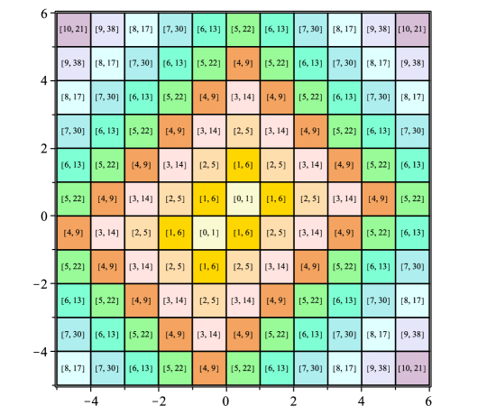
Figure 1: Level sets of the first integral $V$ of $F$ for $\alpha={\pi}/{2}$, given in (3). In each tile $T_{k,\ell}$, the level $V_{k,\ell}$ and the period of the center $p_{k,\ell}$ are indicated, between brackets. The other points in the tile have period $8V_{k,\ell}+4$.

Item $(iv)$ was already proved in [8]. All the geometric description of the dynamics of $F$ given in the other items is new.

Observe that the statement (ii) in the above result can be formalized in the following way: the dynamics of $F$ on each necklace $\{V=c\}\cap\mathcal{U}$ with $c\in{\mathbb{N}}_{0},$ is conjugate with the dynamics of the map

$$\begin{array}[]{lccc}\varphi:&\mathbb{Z}_{4c+2}\times\mathbb{Z}_{q}&\longrightarrow&\mathbb{Z}_{4c+2}\times\mathbb{Z}_{q}\\ &(i,j)&\longrightarrow&(i+c,j+1)\end{array}$$

where $q=2$ if $c$ is odd, and $q=4$ if $c$ is even. This map can be seen as the product of two finite order rotations, its first component gives the dynamics on the discrete deferent formed by the set of centers of tiles, and the second component gives the dynamics on a epicycle. A similar situation is described in statements (ii) of Theorems B and C.

Also notice that a simple check shows that the function $V$ is not a first integral of $F$ on the whole plane, since the relation $V(F)=V$ is not satisfied for some points in $\mathcal{F}={\mathbb{R}}^{2}\setminus\mathcal{U}$.

As a consequence of the above theorem we can easily give a simple algorithm to know the period of each orbit in terms of its initial condition. Recall that given a point $(x,y)\in{\mathbb{R}}^{2}$, $k=\operatorname{E}(x)$, $\ell=\operatorname{E}(y)$ and $V_{k,\ell}=V_{\pi/2}(p_{k,\ell}).$ For the forthcoming cases $\alpha\in\{2\pi/3,\pi/3\},$ from our results a more complicated algorithm could be obtained, but for the sake of brevity, we do not detail it.

Proposition 1.

Any point $(x,y)\in{\mathbb{R}}^{2}$ is a $p$-periodic point of $F$, where:

1. When $x\notin{\mathbb{Z}}$ and $y\notin{\mathbb{Z}}$ and, moreover, either $x-k\neq{1}/{2}$ or $y-\ell\neq{1}/{2}$, then $p=8V_{k,\ell}+2.$ When $x-k={1}/{2}$ and $y-\ell={1}/{2}$, then $p=2V_{k,\ell}+1$ if $V_{k,\ell}$ is even, and $p=4V_{k,\ell}+2$ if $V_{k,\ell}$ is odd.

2. When $x\in{\mathbb{Z}}$ and $y\notin{\mathbb{Z}}$, if $k$ is even, $p=8V_{k,\ell}+4$ and if $k$ is odd, $p=8V_{k-1,\ell}+4.$

3. When $x\notin{\mathbb{Z}}$ and $y\in{\mathbb{Z}}$, if $\ell$ is even, $p=8V_{k,\ell}+4$ and if $\ell$ is odd, $p=8V_{k,\ell-1}+4.$

4. If $x\in{\mathbb{Z}}$ and $y\in{\mathbb{Z}}$, then:

   1. When $k$ is even, $p=8V_{k,\ell}+4$ if $\ell$ is even, and $p=8V_{k,\ell-1}+4$ if $\ell$ is odd.

   2. When $k$ is odd, $p=8V_{k-1,\ell}+4$ if $\ell$ is even, and $p=8V_{k-1,\ell-1}+4$ if $\ell$ is odd.

The statement (d) in the above result is a consequence of Theorem 10. To obtain the result we will identify some tiles, that we will call perfect squares, such that their boundaries (including their edges and all the vertices in $\mathcal{F}$) avoid the discontinuity effects and, therefore, the points on the boundary of such a tile have the same periodic behavior as the interior points, except their centers. To study the periodicity in the rest of the edges (without vertices) we will associate them with an appropriate tile, so that the points in the edge follow the periodic behavior of the interior points. See Section 3.3 for more details.

2.2 The case $\alpha={2\pi}/{3}$

In this case, the map $F$ in (2) is conjugate with the map $G$ in (1) with $\rho=1$, which was studied in [10].

We define $\mathcal{F}_{2\pi/3}$ as the grid formed by the straight lines $y=\sqrt{3}(x-2k),$ $y=\sqrt{3}\ell$ and $y=-\sqrt{3}(x-2m-1)$, with $k,\ell,m\in\mathbb{Z}$ and call ${\mathcal{U}_{2\pi/3}}={\mathbb{R}}^{2}\setminus\mathcal{F}_{2\pi/3}.$ Notice that ${\mathcal{U}_{2\pi/3}}$ is the (open) trihexagonal Euclidean uniform tiling (the tessellation 3.6.3.6 in the notation of [16]), see Figure 2. In fact, each tile in ${\mathcal{U}_{2\pi/3}}$ is defined by

$$\begin{array}[]{rl}T_{k,\ell,m}=&\big{\{}(x,y),\mbox{ such that }\sqrt{3}(x-2k-2)<y<\sqrt{3}(x-2k),\sqrt{3}\ell<y<\sqrt{3}(\ell+1),\\ &\mbox{ and }-\sqrt{3}(x-2m+1)<y<-\sqrt{3}(x-2m-1)\big{\}},\end{array}$$

with $m\in\{k+\ell,k+\ell+1,k+\ell+2\},$ where $k=B(x,y),$ $\ell=C(y)$ and $m=D(x,y),$ being

$$B(x,y)=\operatorname{E}\left({(3x-\sqrt{3}y)}/{6}\right),\,C(y)=\operatorname{E}\left({\sqrt{3}y}/{3}\right)\mbox{ and }D(x,y)=\operatorname{E}\left({(3x+\sqrt{3}y+3)}/{6}\right).$$

Moreover,

• The tile $T_{k,\ell,k+\ell+1}$ is a regular hexagon and its geometric center (simply center, from now on) is the point $p_{k,\ell}=\left(2k+\ell+{3}/{2},\sqrt{3}(\ell+{1}/{2})\right);$

• The tiles $T_{k,\ell,k+\ell}$ and $T_{k,\ell,k+\ell+2}$ are equilateral triangles whose respective centers are $q_{k,\ell}=\left(2k+\ell+{1}/{2},\sqrt{3}(\ell+{1}/{6})\right)$ and $r_{k,\ell}=\left(2k+\ell+{5}/{2},\sqrt{3}(\ell+{5}/{6})\right);$

and the adherence of the union of the three tiles is a parallelogram whose sides are $y=\sqrt{3}\ell\,,y=\sqrt{3}(\ell+1)\,,\,y=\sqrt{3}(x-2k)$ and $y=\sqrt{3}(x-2k-2),$ see Figure 7 and Lemma 13 for more details. Finally, we introduce the function

$$V_{2\pi/3}(x,y)=\max\big{(}\left|B(x,y)-C(y)+D(x,y)\right|,\\ \left|B(x,y)+C(y)+D(x,y)+1\right|-1,\left|-B(x,y)+C(y)+D(x,y)\right|\big{)}.$$ (4)

Observe that its level sets are discrete and $\operatorname{Image}(V_{2\pi/3})=\mathbb{N}_{0}.$ Clearly, $V_{2\pi/3}$ is constant on each tile $T_{k,\ell,m}$ and we denote its value as

$$V_{k,\ell,m}=\max\left(|k-\ell+m|,|k+\ell+m+1|-1,|-k+\ell+m|\right).$$ (5)

Theorem B.

Consider the discrete dynamical system generated by the map $F$ given in (2) with $\alpha=2\pi/3.$ Then:

1. Its critical set is $\mathcal{F}=\mathcal{F}_{2\pi/3}.$

2. The function $V=V_{2\pi/3}$ is a first integral of $F$ on the free-zero set $\mathcal{U}=\mathcal{U}_{2\pi/3}={\mathbb{R}}^{2}\setminus\mathcal{F}_{2\pi/3}.$

   1. Each level set $\{V(x,y)=c\},$ with $c\in 2{\mathbb{N}}_{0}$ even, in $\mathcal{U}$ is a necklace formed by $6c+2$ triangles, see Figure 2. If we identify each triangle with a point (the center, for instance), the DDS restricted to this set is conjugated with the DDS generated by the map $h:{\mathbb{Z}}_{6c+2}\to{\mathbb{Z}}_{6c+2},$ $h(i)=i+2c.$ As a consequence, each tile in this level set is invariant by $F^{3c+1}$ and restricted to this triangle, $F^{3c+1}$ is a rotation of order $3$ around the center of the tile. In particular, all points but the center in each of these tiles have period $9c+3.$

   2. Each level set $\{V(x,y)=c\},$ with $c\in 2{\mathbb{N}}_{0}+1$ odd, in $\mathcal{U}$ is a necklace formed by $3c+1$ hexagons, see Figure 2. If we identify each hexagon with a point, the DDS restricted to this set is conjugated with the DDS generated by the map $h:{\mathbb{Z}}_{3c+1}\to{\mathbb{Z}}_{3c+1},$ $h(i)=i+c.$ As a consequence, each tile in this level set is invariant by $F^{3c+1}$ and restricted to this hexagon, $F^{3c+1}$ is a rotation of order $3$ around the center of the tile. In particular, all points but the center in each of these tiles have period $9c+3.$

3. All orbits with initial condition on $\mathcal{F}$ are periodic with period $9n+3$ for some $n\in{\mathbb{N}}_{0}.$

4. The map $F$ is pointwise periodic. Furthermore, its set of periods is

   $$\operatorname{Per}(F)=\left\{3n+1\mbox{ and }9n+3\mbox{ for all }n\in{\mathbb{N}}_{0}\right\}.$$

Similarly to Theorem A, item $(iv)$ was already known, see [10]. Again, all the geometric description of the dynamics of $F$ given in the other items is new.

From statement (ii), on each necklace, $F$ is conjugate with the product of rotations $\varphi:\mathbb{Z}_{6c+2}\times\mathbb{Z}_{3}\righttoleftarrow$ given by $\varphi(i,j)=(i+2c,j+1)$ when $c$ is even, and $\varphi:\mathbb{Z}_{3c+1}\times\mathbb{Z}_{3}\righttoleftarrow$ given by $\varphi(i,j)=(i+c,j+1)$ when $c$ is odd.

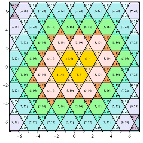
Figure 2: Level sets of the first integral $V$ given in (4). In each tile the level and the period of the center are indicated respectively between brackets.

2.3 The case $\alpha={\pi}/{3}$

In this last case, the map $F$ in (2) is conjugate with the map $G$ in (1) with $\rho=-1$, which was studied in [7].

We consider $\mathcal{F}_{\pi/3}$ the grid formed by the straight lines $y=\sqrt{3}(x-2k-1)$; $y=\sqrt{3}\ell$ and $y=-\sqrt{3}(x-2m)$, with $k,\ell,m\in\mathbb{Z}$ that, again, form a trihexagonal Euclidean uniform tiling which is a translation of the one that appeared in the previous case $\alpha={2\pi}/{3}$, see Figure 3. The interior of each tile is defined by

$$\begin{array}[]{rl}T_{k,\ell,m}=&\big{\{}(x,y),\mbox{ such that }\sqrt{3}(x-2k-1)<y<\sqrt{3}(x-2k+1),\sqrt{3}\ell<y<\sqrt{3}(\ell+1),\\ &\mbox{ and }-\sqrt{3}(x-2m)<y<-\sqrt{3}(x-2m-2)\big{\}}.\end{array}$$

As before, we call ${\mathcal{U}_{\pi/3}}$ the complement of this grid. Any point $(x,y)\in{\mathcal{U}_{\pi/3}}$ belongs (only) to the tile $T_{k,\ell,m}$ with $k=B(x,y),$ $\ell=C(y)$ and $m=D(x,y),$ where

$$B(x,y)=\operatorname{E}\left({(3x-\sqrt{3}y+3)}/{6}\right),\,C(y)=\operatorname{E}\left({\sqrt{3}y}/{3}\right)\mbox{ and }D(x,y)=\operatorname{E}\left({(3x+\sqrt{3}y)}/{6}\right)$$

and now it can be seen that $m=k+\ell-1$ or $m=k+\ell$ or $m=k+\ell+1.$ In this case,

• The tile $T_{k,\ell,k+\ell}$ is a regular hexagon and its center is at the point

  $$p_{k,\ell}=\left(2k+\ell+{1}/{2},\sqrt{3}\ell+{\sqrt{3}}/{2}\right).$$

• The tiles $T_{k,\ell,k+\ell-1}$ and $T_{k,\ell,k+\ell+1}$ are equilateral triangles whose centers are $q_{k,\ell}=\left(2k+\ell-{1}/{2},\sqrt{3}\ell+{\sqrt{3}}/{6}\right)$ and $r_{k,\ell}=\left(2k+\ell+{3}/{2},\sqrt{3}\ell+{5\sqrt{3}}/{6}\right),$ respectively.

We also introduce the following function

$$V_{\pi/3}(x,y)=\max\big{(}\left|B(x,y)-C(y)+D(x,y)\right|,\left|B(x,y)+C(y)+D(x,y)+1\right|-1\\ ,\left|-B(x,y)+C(y)+D(x,y)+1\right|-1\big{)}.$$ (6)

Observe that by construction, it is constant on each tile $T_{k,\ell,m}.$ Hence we can associate to each point in this tile, the value

$$V_{k,\ell,m}=\max\left(|k-\ell+m|,|k+\ell+m+1|-1,|-k+\ell+m+1|-1\right).$$

Our results for this case are collected in the next theorem. We remark that the proof of item $(iii)$ will be the more complicated part of the paper.

Theorem C.

Consider the discrete dynamical system generated by the map $F$ given in (2) with $\alpha=\pi/3.$ Then:

1. Its critical set is $\mathcal{F}=\mathcal{F}_{\pi/3}.$

2. The function $V=V_{\pi/3}$ is a first integral of $F$ on the free-zero set $\mathcal{U}=\mathcal{U}_{\pi/3}={\mathbb{R}}^{2}\setminus\mathcal{F}_{\pi/3}.$

   1. Each level set $\{V(x,y)=c\},$ with $c\in 2{\mathbb{N}}_{0}$ even, in $\mathcal{U}$ is a necklace formed by $3c+2$ hexagons, see Figure 3. If we identify each one of them with a point, the DDS restricted to this set is conjugated with the DDS generated by the map $h:{\mathbb{Z}}_{3c+2}\to{\mathbb{Z}}_{3c+2},$ $h(i)=i+c/2.$ As a consequence, when $c=4j$ (resp. $c=4j+2$), each tile in this level set is invariant by $F^{3c/2+1}$ (resp. $F^{3c+2}$) and restricted to this hexagon, $F^{3c/2+1}$ (resp. $F^{3c+2}$) is a rotation of order $6$ (resp. $3$) around the center of the tile. In particular, all points but the center in each of these tiles have period $9c+6.$

   2. Each level set $\{V(x,y)=c\},$ with $c\in 2{\mathbb{N}}_{0}+1$ odd, in $\mathcal{U}$ is a necklace formed by $6c+4$ triangles, see Figure 1. If we identify each one of them with a point, the DDS restricted to this set is conjugated with the DDS generated by the map $h:{\mathbb{Z}}_{6c+4}\to{\mathbb{Z}}_{6c+4},$ $h(i)=i+c.$ As a consequence, each tile in this level set is invariant by $F^{6c+4}$ and restricted to this triangle, $F^{6c+4}$ is a rotation of order $3$ around the center of the tile. In particular, all points but the center in each of these tiles have period $18c+12.$

3. All orbits with initial condition on $\mathcal{F}$ are periodic with periods $36n+6,$ $18n+9,$ $18n+15$ or $108n+72,$ for some $n\in{\mathbb{N}}_{0},$ for more details see Theorem 22.

4. The map $F$ is pointwise periodic. Furthermore, the set of periods is

   $$\operatorname{Per}(F)= \left\{6n+1;\,12n+8;\,12n+10;\,18n+9;\,18n+15;\,36n+6;\,36n+24;36n+30\right.$$

   $$\left.\mbox{ and }108n+72\mbox{ for all }n\in{\mathbb{N}}_{0}\right\}.$$

Once more, although item $(iv)$ is known, see [7], all the geometric description of the dynamics of $F$ given in the other items is new. From the above result, on each necklace, $F$ is conjugate with the map $\varphi:\mathbb{Z}_{3c+2}\times\mathbb{Z}_{q}\righttoleftarrow$ given by $\varphi(i,j)=(i+c/2,j+1)$, where $q=6$ when $c\equiv 0\,\operatorname{mod}\,(4)$, and $q=3$ when $c\equiv 2\,\operatorname{mod}\,(4)$; or $\varphi:\mathbb{Z}_{6c+4}\times\mathbb{Z}_{3}\righttoleftarrow$ where $\varphi(i,j)=(i+c,j+1)$, when $c$ is odd.

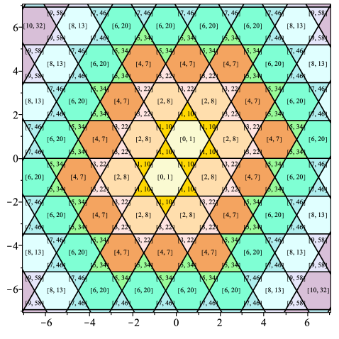
Figure 3: Level sets of the first integral $V$ of $F$ for $\alpha={\pi}/{3}$, given in in (6). In each tile the level and the period of the center are indicated respectively between brackets.

Remark 2.

As we have mentioned, in [14] an infinite number of necklaces of a family of maps that include the ones studied in this work are characterized. We want to note that Theorems A–C show that for our maps all energy levels are necklaces. In particular, in the case $\alpha=\pi/2$ the necklaces studied in [14] correspond to the energy levels whose centers have period $4n+1$ (which are those with even energy level). Let us observe that from Theorem A we know that there are other necklaces whose period is $4n+2$ (those with odd energy level). In the case $\alpha=2\pi/3$, the necklaces in [14] cover all energy levels since all the necklaces have centers of period $3n+1$. In the case $\alpha=\pi/3$ the necklaces in [14] are those whose centers have period $6n+1$. Observe that Theorem C guarantees the existence of much more necklaces.

2.4 The address of a point

We end this section with the concept of address of a point that will be used in the proof of Theorems A, B, C.

Recall that every map in the considered one-parameter family $F$ has discontinuity line $LC_{0}=\{y=0\}$, so we introduce the sets

$$H_{+}=\{(x,y)\in{\mathbb{R}}^{2}:y\geq 0\}\,\mbox{ and }\,H_{-}=\{(x,y)\in{\mathbb{R}}^{2}:y<0\},$$

and we call $F_{+}$ and $F_{-}$ the map $F$ restricted to $H_{+}$ and $H_{-}$ respectively. For any point $(x,y)\in{\mathbb{R}}^{2}$ we define its address $A(x,y)$ as follows:

$$A(x,y)=\left\{\begin{array}[]{ll}+,&\hbox{if $(x,y)\in H_{+}$,}\\ -,&\hbox{otherwise.}\end{array}\right.$$

Moreover for every $n\in\mathbb{N}$, we call the itinerary of length $n$ of the point $(x,y)$ the sequence of $n$ symbols

$$\underline{I}_{n}(x,y)=(A(x,y),A(F(x,y)),\ldots,A(F^{n-1}(x,y))).$$

Notice that if $\underline{I}_{n}(x,y)=(i_{1},\ldots,i_{n})$ then $F^{n}(x,y)=F_{i_{n}}\circ F_{i_{n-1}}\circ\cdots\circ F_{i_{1}}(x,y).$

For instance if $(x,y)\in H_{+}$, $F(x,y)\in H_{-}$ and $F^{2}(x,y)\in H_{-}$, then the length $3$ itinerary of the point is $\{+,-,-\}$, and $F^{3}(x,y)=F_{-}\circ F_{-}\circ F_{+}(x,y).$

Lemma 3.

Let $\underline{J}_{n}=(i_{1},\ldots,i_{n})$ be a sequence of symbols of length $n$ with $i_{i}\in\{+,-\}$ and consider the set $B(\underline{J}_{n})=\{(x,y)\in{\mathbb{R}}^{2}\mbox{ such that }\underline{I}_{n}(x,y)=\underline{J}_{n}\}$. Then $B(\underline{J}_{n})$ is convex. Moreover $F^{n}$ restricted to $B(\underline{J}_{n})$ is an affine map.

Proof.

The proof of the convexity follows easily by induction. If $n=1,$ $B(\underline{J}_{n})$ is either $H_{+}$ or $H_{-}$ both convex sets. Assume that the result holds for sequences of length $n-1$ and set $\underline{J}_{n-1}=(i_{1},\ldots,i_{n-1}).$ Therefore we have

$$B(\underline{J}_{n})=\{(x,y)\in B(\underline{J}_{n-1}):F^{n-1}(x,y)\in H_{i_{n}}\}.$$

Moreover, $F^{n-1}$ restricted to $B(\underline{J}_{n-1})$ is the affine map $G=F_{i_{n-1}}\circ\ldots\circ F_{i_{1}}.$ So we have

$$B(\underline{J}_{n})=B(\underline{J}_{n-1})\cap G^{-1}(H_{i_{n}}).$$

This fact proves that $B(\underline{J}_{n})$ is convex because it is the intersection of two convex sets. This ends the inductive proof of convexity. Furthermore, $F^{n}(x,y)=F_{i_{n}}\circ F_{i_{n-1}}\circ\cdots\circ F_{i_{1}}(x,y),$ for all $(x,y)\in B(\underline{J}_{n}),$ showing that $F^{n}$ restricted to $B(\underline{J}_{n})$ is an affine map.    

3 Proof of Theorem A

3.1 Preliminaries

We start by determining the set of tile centers, $p_{k,\ell}$, such that $V(p_{k,\ell})=c$ for $c\in{\mathbb{N}}_{0}.$ First, we observe that there are two tiles corresponding to the level set $c=0$. These two tiles contain the two fixed points of $F$ which are: $p_{0,0}=\left({1}/{2},{1}/{2}\right)$ that belongs to the tile $T_{0,0}=(0,1)\times(0,1)$ and $p_{-1,-1}=\left(-{1}/{2},-{1}/{2}\right)$ that belongs to $T_{-1,-1}=(-1,0)\times(-1,0).$ It is easy to see that these two tiles are invariant. To describe the rest of level sets, we denote $\mathcal{Q}_{1}=\{(x,y)\in{\mathbb{R}}^{2}:x<0,y>0\},$ $\mathcal{Q}_{2}=\{(x,y)\in{\mathbb{R}}^{2}:x>0,y>0\},$ $\mathcal{Q}_{3}=\{(x,y)\in{\mathbb{R}}^{2}:x>0,y<0\},$ and $\mathcal{Q}_{4}=\{(x,y)\in{\mathbb{R}}^{2}:x<0,y<0\}.$

Lemma 4.

For each level set $\{V=c\}$ with $c\in{\mathbb{N}}_{0}$ there are $4c+2$ centers $p_{k,\ell}$. Furthermore, for each natural number $c\geq 1$ we have:

1. $\{p_{k,\ell}:V_{k,\ell}=c\}\cap\mathcal{Q}_{1}=\{(k+{1}/{2},\ell+{1}/{2}):l=k+c,k=-c,-c+1,\ldots,-1\}.$ We denote by $X_{1},X_{2},\ldots,X_{c}$ these $c$ centers for $k=-c,-c+1,\ldots,-1$ respectively. Every one of them lies on the straight line $y=x+c.$

2. $\{p_{k,\ell}:V_{k,\ell}=c\}\cap\mathcal{Q}_{2}=\{(k+{1}/{2},\ell+{1}/{2}):l=-k+c,k=0,1,\ldots,c\}.$ We denote by $X_{c+1},X_{c+2},\ldots,X_{2c+1}$ these $c+1$ centers for $k=0,1,\ldots,c$ respectively. Every one of them lies on the straight line $y=-x+c+1.$

3. $\{p_{k,\ell}:V_{k,\ell}=c\}\cap\mathcal{Q}_{3}=\{(k+{1}/{2},\ell+{1}/{2}):l=k-c,k=0,1,\ldots,c-1\}.$ We denote by $X_{2c+2},X_{2c+3},\ldots,X_{3c+1}$ these $c$ centers for $k=c-1,c-2,\ldots,0$ respectively. Every one of them lies on the straight line $y=x-c.$

4. $\{p_{k,\ell}:V_{k,\ell}=c\}\cap\mathcal{Q}_{4}=\{(k+{1}/{2},\ell+{1}/{2}):l=-k-c-2,k=-1,-2,\ldots,-c-1\}.$ We denote by $X_{3c+2},X_{3c+3},\ldots,X_{4c+2}$ these $c+1$ centers for $k=-1,-2,\ldots,-c-1$ respectively. Every one of them lies on the straight line $y=-x-c-1.$

Proof.

In order to prove $(a)$ we begin by considering the points $(k+{1}/{2},k+c+{1}/{2})$ with $-c\leq k\leq-1.$ Then $V_{k,k+c}=\max\left(|2k+c+1|-1,c\right).$ The inequality $-c\leq k\leq-1$ implies $-c+1\leq 2k+c+1\leq c-1,$ i.e. $|2k+c+1|\leq c-1.$ Therefore $|2k+c+1|-1\leq c-2$ and consequently $V_{k,k+c}=c.$ Clearly, $k+{1}/{2}<0$ and $k+c+{1}/{2}>0$, and hence the points belong to $\mathcal{Q}_{1}$.

To see the other inclusion take $(k+{1}/{2},\ell+{1}/{2})\in\mathcal{Q}_{1}$ with $V_{k,\ell}=c$. We have to prove that $\ell=k+c$ and $-c\leq k\leq-1.$ We know that $k<0,$ $\ell\geq 0$ which easily implies that $\ell>k.$ Hence $|\ell-k|=\ell-k$, and $\ell+k<\ell<\ell-k.$ Then

$$V_{k,\ell}=\max\left(\left|k+\ell+1\right|-1,\left|k-\ell\right|\right)=\max\left(\left|k+\ell+1\right|-1,\ell-k\right).$$

Consider the following two cases:

1. Assume $\ell+k+1\geq 0.$ Then $V_{k,\ell}=\max(\ell+k,\ell-k)=\ell-k$ because $\ell+k<\ell<\ell-k.$ It implies that $\ell-k=c,$ that is $\ell=k+c.$ Furthermore, since $\ell=k+c$ and $\ell\geq 0$ we get $k\geq-c$.

2. Assume $\ell+k+1<0.$ Then $V_{k,\ell}=\max(-\ell-k-2,\ell-k).$ Since $(\ell-k)-(-\ell-k-2)=2\ell+2=2(\ell+1)$ and $\ell+1>0$ also $\ell=k+c$ and the result follows as above.

The proof of statements $(b),(c)$ and $(d)$ follows using the same easy arguments.     

In Figure 4 we show the points $p_{k,\ell}$ in the levels $c=2$ and $c=3,$ respectively.

 

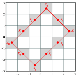
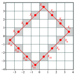
Figure 4: The centers in the levels $c=2$ and $c=3.$

3.2 Proof of items (i) and (ii) of Theorem A: dynamics on the zero-free set

Recall that in this case, $F(x,y)=(y,-x+\operatorname{sign}(y)),$ $F_{+}(x,y)=(y,-x+1)$ and $F_{-}(x,y)=(y,-x-1).$ We will split our proof of items $(i)$ and $(ii)$ of Theorem A in several lemmas and propositions.

We start facing the dynamics of the center points of the tiles, or in other words, the dynamics among the beads of each necklace, that as we will prove will be invariant under the map $F.$

Lemma 5.

Fixed $c\in\mathbb{N}$, consider the centers $X_{1},X_{2},\ldots,X_{4c+2}$ which belong to the level set $\{V=c\}.$ Then

$$F(X_{i})=X_{j}\,\,\text{with}\,\,j\equiv i+c\,\,\operatorname{mod}\,\,(4c+2).$$ (7)

Proof.

Consider $i=1,2,\ldots,c$, then $X_{i}\in\mathcal{Q}_{1}.$ From Lemma 4 we know that every one of these centers is $\left(k+{1}/{2},k+c+{1}/{2}\right)$ with $k=-c,-c+1,\ldots,-1.$ Since they belong to $H_{+}$ we have

$$F(X_{i})=F_{+}\left(k+{1}/{2},k+c+{1}/{2}\right)=\left(k+c+{1}/{2},-k+{1}/{2}\right).$$

Denoting $\bar{k}=k+c$ we see that $\left(k+c+{1}/{2},-k+{1}/{2}\right)=\left(\bar{k}+{1}/{2},-\bar{k}+c+{1}/{2}\right)$ which satisfies the condition (b) of the Lemma 4. When $k$ runs from $-c$ to $-1$ (corresponding with the points $X_{1},X_{2},\ldots,X_{c}$), then $\bar{k}$ runs from $0$ to $c-1$ (corresponding with the points $X_{c+1},X_{c+2},\ldots,X_{2c}$). Hence we have proved (7) for $i=1,2,\ldots,c.$

If $i=c+1$ then $X_{c+1}=\left({1}/{2},c+{1}/{2}\right),$ hence $F(X_{c+1})=F_{+}(X_{c+1})=\left(c+{1}/{2},{1}/{2}\right)=X_{2c+1}.$

The proof for $i=c+2,c+3,\ldots,2c+1$ is done in a similar way, and also for the rest of values of $i=2c+2,\ldots,4c+2$, but taking into account that in these cases $F(X_{i})=F_{-}(X_{i}).$

 

As a consequence of Lemma 5 the center points of a level set form an invariant set and we can prove that the function $V_{\pi/2}$ defined in (3) is a first integral of $F.$

Proof of the first part of item $(ii)$ of Theorem A.

We start proving that the function $V=V_{\pi/2}$ defined in (3) is a first integral of $F$ on the set ${\mathcal{U}}={\mathcal{U}}_{\pi/2}$.

Consider a point $(x,y)\in{\mathcal{U}},$ then $(x,y)\in T_{k,\ell}$ for a certain $k,\ell$ and by definition we know that $V(x,y)=V(p_{k,\ell}).$ From Lemma 5 we know that $F(p_{k,\ell})=p_{\bar{k},\bar{\ell}}$ with $V(p_{k,\ell})=V(p_{\bar{k},\bar{\ell}}).$ On the other hand, since each tile is entirely contained in $H_{+}\setminus\{y=0\}$ or in $H_{-},$ $F(T_{k,\ell})=F_{+}(T_{k,\ell})$ or $F(T_{k,\ell})=F_{-}(T_{k,\ell}).$ Since $F_{+}$ and $F_{-}$ are rotations (thus isometries) we get that $F$ sends tiles to tiles. In particular $F(T_{k,\ell})=T_{\bar{k},\bar{\ell}}$ and hence $V(x,y)=V(p_{k,\ell})=V(p_{\bar{k},\bar{\ell}})=V(F(x,y)).$    

Now we are able to describe the dynamics of the center points and, in particular, to prove that they are periodic.

Proposition 6.

Every center $p_{k,\ell}$ is a periodic point of $F.$ Furthermore, setting $V_{k,\ell}=c$ we have that when $c$ is even (resp. odd), then $p_{k,\ell}$ has period $2c+1$ (resp. $4c+2$).

Proof.

Fix a level $\{V=c\}$ with $c\in\mathbb{N}.$ From Lemma 4 we know that on $\{V=c\}$ there are $4c+2$ different centers. From Lemma 5, we know that $F$ sends centers to centers, that is, the set $\{X_{1},X_{2},\ldots,X_{4c+1}\}$ is invariant by $F.$ Hence, given a center $X_{i_{1}}$ of the previous set we can study the sequence $X_{i_{1}}\overset{F}{\longrightarrow}X_{i_{2}}\overset{F}{\longrightarrow}X_{i_{3}}\overset{F}{\longrightarrow}\cdots.$ Since the orbit of every center has a finite number of elements and, since $F$ is a bijective map and therefore the orbit of $X_{i_{1}}$ can not be preperiodic, we get that $X_{i_{p}}=X_{i_{1}}$ for a certain $p$, and therefore it is periodic. Clearly the period must be less or equal to $4c+2.$

From Lemma 5, the map $F$ restricted to $\{X_{1},X_{2},\ldots,X_{4c+1}\}$ is conjugate to the map $h:{\mathbb{Z}}_{4c+2}\longrightarrow{\mathbb{Z}}_{4c+2}$ defined by $h(i)=i+c.$ Then

$$F^{p}(X_{i})=X_{i}\Leftrightarrow h^{p}(i)=i\Leftrightarrow i+cp\equiv i\,\,\operatorname{mod}\,\,(4c+2)\Leftrightarrow\exists\,n\in{\mathbb{N}}\mbox{ s.t. }cp=n(4c+2).$$

Assume that $c=2k$ is an even number. Then $2kp=n(8k+2)\Leftrightarrow kp=n(4k+1).$ It implies that $p$ is a multiple of $4k+1=2c+1.$ Since $p\leq 4c+2$ we get that $p=2c+1$ or $p=4c+2.$ But we observe that the orbit of $X_{i}$ only contains some points $X_{j}$ with $j$ having the same parity of $i.$ Hence, we get two different periodic orbits, each one of them of period $2c+1.$

Assume that $c=2k+1$ is an odd number. Then $(2k+1)p=n(8k+6).$ It implies that $p$ is a multiple of $8k+6=4c+2.$ Hence $p=4c+2.$

 

We introduce now the concept of itinerary map associated with a center.

Definition 7.

Fix $c\in\mathbb{N}$ and consider one of the centers of the tiles $X_{j}$ for some $j=1,2,\ldots,4c+2,$ with $V(X_{j})=c.$ Since $X_{j}$ is $p$-periodic with $p=2c+1$ or $p=4c+2$ depending on whether $c$ is even or it is odd, if we consider its itinerary of length $p$: $\underline{I}_{p}=(i_{1},i_{2},\ldots,i_{p})$ we have that $F^{p}(X_{j})=F_{i_{p}}\circ F_{i_{p-1}}\circ\cdots\circ F_{i_{1}}(X_{j})=X_{j}.$ We denote this composition by $I_{j}=F_{i_{p}}\circ F_{i_{p-1}}\circ\cdots\circ F_{i_{1}}$ and we call it the itinerary map associated with $X_{j}.$

For instance, if $c=2$ then the center $X_{1}$ is $5$-periodic and its orbit is

$$X_{1}\overset{F_{+}}{\longrightarrow}X_{3}\overset{F_{+}}{\longrightarrow}X_{5}\overset{F_{+}}{\longrightarrow}X_{7}\overset{F_{-}}{\longrightarrow}X_{9}\overset{F_{-}}{\longrightarrow}X_{1}$$

This can be easily obtained using the formula (7) in Lemma 5 (see also Figure 4). Hence $\underline{I}_{5}(X_{1})=(+,+,+,-,-)$ and its itinerary map is $I_{1}=F_{-}^{2}\circ F_{+}^{3}$.

When $c=3,$ then using again formula (7) in Lemma 5 (see again Figure 4) we get:

$$X_{1} \overset{F_{+}}{\longrightarrow}X_{4}\overset{F_{+}}{\longrightarrow}X_{7}\overset{F_{+}}{\longrightarrow}X_{10}\overset{F_{-}}{\longrightarrow}X_{13}\overset{F_{-}}{\longrightarrow}X_{2}\overset{F_{+}}{\longrightarrow}X_{5}\overset{F_{+}}{\longrightarrow}X_{8}$$

$$\overset{F_{-}}{\longrightarrow}X_{11}\overset{F_{-}}{\longrightarrow}X_{14}\overset{F_{-}}{\longrightarrow}X_{3}\overset{F_{+}}{\longrightarrow}X_{6}\overset{F_{+}}{\longrightarrow}X_{9}\overset{F_{-}}{\longrightarrow}X_{12}\overset{F_{-}}{\longrightarrow}X_{1},$$

and hence the itinerary map of $X_{1}$ is $I_{1}=F_{-}^{2}\circ F_{+}^{2}\circ F_{-}^{3}\circ F_{+}^{2}\circ F_{-}^{2}\circ F_{+}^{3}$.

Lemma 8.

Fixed $c\in\mathbb{N},$ consider the centers $X_{1},X_{2},\ldots,X_{4c+2}$ lying in the level set $\{V=c\}.$ Then for all $j=1,2,\ldots,4c+2$, the itinerary map $I_{j}$ is a rotation centered at $X_{j}$ of order $4$ if $c$ is even (angle ${\pi}/{2}$), and of order $2$ if $c$ is odd (angle $\pi$). In particular $X_{j}$ is an isolated fixed point of $I_{j}$.

Proof.

We already know that $I_{j}(X_{j})=X_{j}.$ We write

$$F(x,y)=A\cdot\begin{pmatrix}x-\operatorname{sign}(y)\\ y\end{pmatrix}\mbox{ where }A=R_{{\pi}/{2}}=\begin{pmatrix}0&1\\ -1&0\end{pmatrix}.$$

If $c=2k$, then by using Proposition 6 we have that $X_{j}$ is $(2c+1)$-periodic, hence, using also that $A^{4}=\operatorname{Id}$ we obtain

$$I_{j}(x,y)=A^{2c+1}\begin{pmatrix}x\\ y\end{pmatrix}+v_{j}=A^{4k+1}\begin{pmatrix}x\\ y\end{pmatrix}+v_{j}=A\begin{pmatrix}x\\ y\end{pmatrix}+v_{j}$$

for a certain $v_{j}\in{\mathbb{R}}^{2}$. Hence $I_{j}$ is a rotation of order $4$ centered at $X_{j}$. Since it has a unique fixed point (as $\operatorname{Rank}(A-\operatorname{Id})=2$) then the center of this rotation is $X_{j}$.

If $c=2k+1$, then $X_{j}$ has period $4c+2,$ hence using that $A^{2}=R_{\pi}=-\operatorname{Id}$, we have:

$$I_{j}(x,y)=A^{4c+2}\begin{pmatrix}x\\ y\end{pmatrix}+w_{j}=A^{8k+6}\begin{pmatrix}x\\ y\end{pmatrix}+w_{j}=A^{2}\begin{pmatrix}x\\ y\end{pmatrix}+w_{j},$$

for a certain $w_{j}\in{\mathbb{R}}^{2}.$ By using the same argument as before, $I_{j}$ is a rotation of order $2$ centered at $X_{j}$.    

To end the technical results we establish the next lemma which ensures the all the points in a tile have the same itinerary of arbitrary length:

Lemma 9.

All the points in a given tile $T_{k,\ell}$ have the same itinerary of length $n\in\mathbb{N}$ for every $n\in\mathbb{N}.$

Proof.

Fix $n\in\mathbb{N}$, and suppose that there exist two points $p$ and $q$ in $T_{k,\ell}$ with different itinerary of length $n$ and let $j\leq n-1$ the first time that $A(F^{j}(p))\neq A(F^{j}(q)).$ That is $p$ and $q$ have the same itinerary of length $j$ but $F^{j}(p)$ and $F^{j}(q)$ have different addresses. From Lemma 3 we have that all the points in the segment $\overline{p\,q}$ have the same itinerary of length $j$ and therefore $F^{j}$ restricted to $\overline{p\,q}$ is continuous. Since $F^{j}(p)$ and $F^{j}(q)$ have different addresses it follows that there exists a point $r\in\overline{p\,q}$ such that $F^{j}(r)\in LC_{0}.$ A contradiction because since $T_{k,\ell}$ is also convex, $r\in T_{k,\ell}$ and must be zero-free.    

We can now prove item $(i),$ that is, the zero-free points are exactly the points $\mathcal{U}=\mathcal{U}_{\pi/2},$ which belong to the tiles.

Proof of item $(i)$ of Theorem A.

We have already noticed that the zero-free set is included in ${\mathcal{U}_{\pi/2}}.$ Now we are going to see that the boundaries of the tiles are formed by points which are not zero-free. Consider a point $p=(k,y)$ where $\ell\leq y\leq\ell+1$ for a certain $k,\ell\in{\mathbb{Z}}.$ Then $p$ belongs to the right-boundary of $T_{k-1,\ell}$ and to the left boundary of $T_{k,\ell}.$ Consider also the segment $\overline{rs}$ where $r=(k-1/2,y)$ and $s=(k+1/2,y).$ From Lemma 9 the itinerary of any length of $r$ coincides with the itinerary of the same length of $p_{k-1,l}$ and the itinerary of any length of $s$ coincides with the corresponding itinerary of $p_{k,l}.$ Since $p_{k-1,l}$ and $p_{k,l}$ have different infinite itineraries, there exists $j$ such that $\underline{I}_{j}(r)=\underline{I}_{j}(s)$ but $A(F^{j}(r))\neq A(F^{j}(s).$ Now from Lemma 3 it follows that there exists $t\in\overline{rs}$ such that $F^{j}(t)\in LC_{0}.$ Clearly this point must be $p.$

If we consider a point which belongs to a horizontal boundary of two consecutive tiles, then its iterate belongs to a vertical boundary of two consecutive tiles and then we can apply the above result.    

Continuation of the proof of item $(ii)$ of Theorem A.

Consider the tile $T_{k,\ell}$. Let $X_{j}$ be its center. By Proposition 6 it is a $p$-periodic point, and by Lemma 9 all the points in the tile have the same itinerary of length $p$, hence $\left.F^{p}\right|_{T_{k,\ell}}=I_{j}.$ Moreover, by Lemma 8, on each tile $I_{j}$ is a rotation centered at $X_{j}$ of the order established in the statement.

Assume that $V_{k,\ell}=c$ with $c$ an even number. We have already proved that each center $X_{j}$ in this level set has period $2c+1$ (see Proposition 6). The points in the orbit of $X_{j}$ are points $X_{i}$ with $i$ having the same parity of $j$ (see Lemma 5). Hence we have two orbits, the first one formed by $X_{1},X_{3},\ldots,X_{4c+1}$ and the second one formed by $X_{2},X_{4},\ldots,X_{4c+2}$, and therefore we know the period of the centers of the tiles.

The period of all the points of the tiles $T_{k,\ell}$ but the centers is a consequence that we have proved that $\left.F^{p}\right|_{T_{k,\ell}}=I_{p_{k,\ell}},$ where $I_{p_{k,\ell}}$ is the itinerary map of $p_{k,\ell}$, which is a rotation of order $4,$ see again Lemma 8.

When $V_{k,\ell}=c$ with $c$ an odd number the proof is similar.    

3.3 Proof of item $(iii)$ of Theorem A: dynamics on the non zero-free set

Following the notation introduced in Lemma 4, for any fixed energy level $c$ of $V,$ there are $4c+2$ tiles with centers $X_{1},X_{2},\ldots,X_{4c+2}$. Let us denote $T_{j}$ to the tile with center $X_{j}$. Also, for a fixed energy level $c$, we denote by $Q_{j}$ the closed square formed by the tile $T_{j}$ and its boundary, that is $Q_{j}=T_{j}\cup\partial T_{j}$.

For each energy level $c$ even, we will call the squares $Q_{1},Q_{3},\ldots,Q_{4c+1}$ perfect squares because, as we will see, these closed squares evolve avoiding the discontinuity effects of $F.$

Clearly every edge of a square is also an edge of the consecutive square. The perfect squares are positioned as Figure 5 displays, the perfect squares being the red ones.

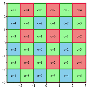
Figure 5: Position of the perfect squares in red. The green tiles correspond to odd energy levels and the blue ones correspond to the even energy levels such that their corresponding squares are not perfect. The borders and the vertices are highlighted with the color of the tile having the same itinerary map. The level set $\{V=c\}$ is indicated in each square.

From the above figure we see that it is enough to prove the periodicity of the points on the boundary of the perfect squares and the periodicity of the points on the boundary on the squares of odd levels which are not in the boundary of the perfect squares.

Our result also will ensure that the points of the border (including the vertices) of any perfect square are periodic with the same period as the points of the tile corresponding to the perfect square (excluding the center). Observe that any vertex point in $\mathcal{F}$ belongs uniquely to a perfect square. Hence the result will characterize the dynamics of all the vertices. The rest of the non-zero points are periodic with the same period as the points of the adjacent tile (excluding the center) with odd energy levels. See again Figure 5.

Item $(iii)$ of Theorem A is a straightforward consequence of the next theorem.

Theorem 10.

Consider the level set $V=c$.

1. If $c$ is an even number, then every point on the boundary of the squares $Q_{1},Q_{3},\ldots,Q_{4c+1}$ is a $(8c+4)$-periodic point.

2. If $c$ is an odd number, then when $j$ is odd (resp. even) the two horizontal (resp. vertical) edges of $Q_{j},$ without the vertices, are formed by $(8c+4)$-periodic points.

Prior to proving the result we stress the following fact:

Remark 11.

On every point in $H_{+}$ the map $F=F_{+}$. Hence, for all $j=1,2,\ldots,2c+1,$ we have that $F(Q_{j})=F_{+}(Q_{j})=Q_{i}$ with $i\equiv j+c$ mod $4c+2$ (see Lemmas 5 and 9). Analogously, for $i=2c+3,\ldots,4c+1$ we have $F(Q_{j})=F_{-}(Q_{j})=Q_{i}$ with $i\equiv j+c$ mod $4c+2$, since these squares are contained in $H_{-}$. Observe, however, that the situation for the squares $Q_{2c+2}$ and $Q_{2c+4}$ is quite different because on the top edge of these two squares $F=F_{+}$ while in the rest of the square $F=F_{-}$. In Figure 6, we display the position of the tiles corresponding with the centers $X_{1}$, $X_{2c+1}$, $X_{2c+2}$ and $X_{4c+2}$ with respect to the discontinuity line $LC_{0}$.

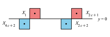
Figure 6: Position of the squares $Q_{1}$, $Q_{2c+1}$, $Q_{2c+2}$ and $Q_{4c+2}$, together with its centers, for any level set $V=c.$

Proof of Theorem 10.

Consider the squares $Q_{1},Q_{3},\ldots,Q_{4c+1}$ for $c$ even, that is, the perfect squares on this level. The only squares in this particular collection $Q_{j}$ with $j$ odd which intersect $y=0$ are $Q_{1}$ and $Q_{2c+1}.$ But from Remark 11 we know that $F(Q_{j})=Q_{k}$ with $k\equiv j+c$ mod $4c+2$ for all $j$ odd, including the cases with $j=1$ and $j=2c+1.$ In particular this implies that this set of squares is invariant. In consequence, by continuity, the points in the boundary of $Q_{j}$ inherit the dynamics of the points in $T_{j}\setminus X_{j}$ and, therefore, they are periodic with period $4(2c+1)$. Furthermore, $\left.F^{2c+1}\right|_{Q_{j}}$ is a rotation of order 4.

Now assume that $c$ is odd. We notice that the squares $Q_{1},Q_{3},\ldots,Q_{4c+1}$ (resp. $Q_{2},Q_{4},$ $\ldots,Q_{4c+2}$) share every vertical (resp. horizontal) edge with an edge of a perfect square, which we already know is periodic. Hence we need to follow the dynamics of their horizontal (resp. vertical) edges or, in other words, the dynamics of $\widetilde{Q}_{j}=Q_{j}\setminus\{$ its vertical edges, including the vertices$\}$ (resp. $\widetilde{Q}_{j}=Q_{j}\setminus\{$its horizontal edges, including the vertices$\}$).

Since now $X_{1},X_{2},\ldots,X_{4c+2}$ belong to the same periodic orbit, the set of corresponding squares contains $\widetilde{Q}_{2c+2}$ and $\widetilde{Q}_{4c+2}.$ The result will be proved if we can ensure the invariance of the set of squares $\widetilde{Q}_{j}$. In order to do this, we must ensure that the edges we are studying are not pre-images of the top edges of the squares $Q_{2c+2}$ and $Q_{4c+2}.$ So, first, we study for which values of $p,$ $F^{p}(X_{j})=X_{2c+2}$ or $F^{p}(X_{j})=X_{4c+2}.$

• From Lemma 5 we have $F^{p}(X_{j})=X_{2c+2}$ if and only if $j+pc\equiv 2c+2$ mod $4c+2$, that is if there exists $n\in{\mathbb{N}}$ such that $j+pc=2c+2+n(4c+2).$ Hence $j+pc$ is an even number and since $c$ is odd we get that $p$ and $j$ have the same parity.

• Analogously, $F^{p}(X_{j})=X_{4c+2}$ if and only if $j+pc\equiv 0$ mod $4c+2$, which means that there exists $n\in{\mathbb{N}}$ such that $j+pc=n(4c+2).$ As before $p$ and $j$ have the same parity.

Assume that $j$ is odd, and let the $p$-iterate of $Q_{j}$ be the first one that reaches $Q_{2c+2}$ (or $Q_{4c+2}$). Since it is the first time that the images of $Q_{j}$ intersect $\{y=0\}$, we can still apply the arguments in the proof of Lemma 8 and therefore $F^{p}|_{Q_{j}}$ is an even-order rotation. Thus, since $p$ is also odd, the horizontal edges of $Q_{j}$ are mapped via $F^{p}$ to the vertical edges of $Q_{2c+2}$ (or $Q_{4c+2}$). Therefore $F^{p}(\widetilde{Q}_{j})=\widetilde{Q}_{2c+2}$ (or $\widetilde{Q}_{4c+2}$). It implies that for all $j$ odd, $F(\widetilde{Q}_{j})=\widetilde{Q}_{j+c}.$

The same arguments work when $j$ is even: $p$ is even too and $F^{p}$ sends the vertical edges of $Q_{j}$ to the vertical edges of $Q_{2c+2}$ (or $Q_{4c+2}$). So also $F(\widetilde{Q}_{j})=\widetilde{Q}_{j+c}$ for every $j$ even.

The condition $F(\widetilde{Q}_{j})=\widetilde{Q}_{j+c}$ implies that, by continuity, the points in the edges under study of $Q_{j}$ inherit the dynamics of the points in $T_{j}\setminus X_{j}$, which are periodic with period $2(4c+1)$.    

Consider the square $Q_{k,\ell}=T_{k,\ell}\cup\partial T_{k,\ell}$, and set $c=V_{k,\ell}$; then, we will say that the square has odd label (resp. even label) if $Q_{k,\ell}=Q_{j}$ for an odd value $j$ (resp. even) in the order introduced in Lemma 4. Observe that, in particular, with the proof of Theorem 10 we also have proved the following result that gives the dynamics of $F$ on all the points in $\mathcal{F}$.

Corollary 12.

Consider the square $Q_{k,\ell}=T_{k,\ell}\cup\partial T_{k,\ell}$, and set $c=V_{k,\ell}$, then:

1. If $c$ is even, and the square has odd label then $Q_{k,\ell}$ is invariant under the action of the map $F^{2c+1}$, and $\left.F^{2c+1}\right|_{Q_{k,\ell}}$ is a rotation of order $4$ centered at $p_{k,\ell}$; as a consequence the edges of these $Q_{k,\ell}$ are formed by $4(2c+1)-$periodic points.

2. If $c$ is odd, and the square has odd label (resp. even label) then the horizontal (resp. vertical) edges (excluding the vertices) are invariant under the action of the map $F^{4c+2}$ which is also a rotation of order $2$ centered at $p_{k,\ell}$ on that edges (excluding the vertices); as a consequence the edges of these squares which are not edges of a perfect square are formed by $2(4c+2)-$periodic points.

Remember that if the square has even energy level and even label we treat their boundaries as being part of the boundary of the adjacent odd-energy level tile.

3.4 Proof of item $(iv)$ of Theorem A

The proof simply follows by collecting the results of the previous items.

4 Proof of Theorem B

4.1 Preliminaries

For each tile $T_{k,\ell,m},$ we start determining $m$ in terms of $k$ and $\ell.$

Lemma 13.

Any point $(x,y)\in\mathcal{U}={\mathcal{U}_{2\pi/3}}$ belongs to a tile $T_{k,\ell,m}$ where either, $m=k+\ell$ or $m=k+\ell+1$ or $m=k+\ell+2.$

Proof.

From the inequalities $k<{x}/{2}-{\sqrt{3}y}/{6}<k+1$ and $\ell<{\sqrt{3}y}/{3}<\ell+1$ it follows that ${1}/{2}+k+\ell<{x}/{2}+{\sqrt{3}y}/{6}+{1}/{2}<k+\ell+{5}/{2}.$ Hence $m=\operatorname{E}({x}/{2}+{\sqrt{3}y}/{6}+{1}/{2})$ is either $m=k+\ell,$ $m=k+\ell+1$ or $m=k+\ell+2.$    

In fact, the set of points satisfying $k<{x}/{2}-{\sqrt{3}y}/{6}<k+1$ and $\ell<{\sqrt{3}y}/{6}<\ell+1$ form a parallelogram whose sides are $y=\sqrt{3}\ell\,,y=\sqrt{3}(\ell+1)\,,\,y=\sqrt{3}(x-2k)$ and $y=\sqrt{3}(x-2k-2).$ From the proof of the above lemma we see that

1. $m=k+\ell\Leftrightarrow k+\ell+{1}/{2}<{x}/{2}+{\sqrt{3}y}/{6}+{1}/{2}<k+\ell+1\Leftrightarrow\sqrt{3}(-x+2k+2\ell)<y<\sqrt{3}(-x+2k+2\ell+1)$

2. $m=k+\ell+1\Leftrightarrow k+\ell+1<{x}/{2}+{\sqrt{3}y}/{6}+{1}/{2}<k+\ell+2\Leftrightarrow\sqrt{3}(-x+2k+2\ell+1)<y<\sqrt{3}(-x+2k+2\ell+3)$

3. $m=k+\ell+2\Leftrightarrow k+\ell+2<{x}/{2}+{\sqrt{3}y}/{6}+{1}/{2}<k+\ell+\frac{5}{2}\Leftrightarrow\sqrt{3}(-x+2k+2\ell+3)<y<\sqrt{3}(-x+2k+2\ell+4)$

Denoting by $L_{1}=\{y=\sqrt{3}(-x+2k+2\ell)\},L_{2}=\{y=\sqrt{3}(-x+2k+2\ell+1)\},L_{3}=\{y=\sqrt{3}(-x+2k+2\ell+3)\}$ and $L_{4}=\{y=\sqrt{3}(-x+2k+2\ell+4)\},$ we can draw its graphics in Figure 7.

Figure 7: The tiles $T_{k,\ell,k+\ell}\cup T_{k,\ell,k+\ell+1}\cup T_{k,\ell,k+\ell+2}$ when $\alpha={2\pi}/{3}.$

In Figure 7, we can see that the parallelogram has been partitioned into three sets: two triangles and one hexagon. Thus, we have proved the following lemma, where we use the notation introduced in Section 2.2.

Lemma 14.

Let $T_{k,\ell,m}$ be one tile of $\mathcal{U}_{2\pi/3}=\mathcal{U}$.

1. If $m=k+\ell$ or $m=k+\ell+2$, then $T_{k,\ell,m}$ is a triangle whose center is either $q_{k,\ell}$ or $r_{k,\ell},$ respectively.

2. If $m=k+\ell+1$ then $T_{k,\ell,m}$ is a hexagon whose center is $p_{k,\ell}.$

4.2 Proof of items $(i)$ and $(ii)$: dynamics on the zero-free set

As in the case $\alpha=\pi/2$ we split the proof of these two items into several lemmas and propositions. Here there is an added difficulty, there are tiles with hexagonal shape and others with triangular shape. We study them separately.

4.2.1 Dynamics on the hexagonal tiles. The case $m=k+\ell+1$

From Lemma 14 the tile $T_{k,\ell,k+\ell+1}$ is a regular hexagon. Set $V_{k,\ell}$ for the value of $V$ on $T_{k,\ell,k+\ell+1}$. Then $V_{k,\ell}=V_{k,\ell,k+\ell+1}=\max\left(|2k+1|,2|k+\ell+1|-1,|2\ell+1|\right).$ The next two results characterize the set of centroids of the hexagons, that is their number and geometric locus, for this case.

Lemma 15.

Let $m=k+\ell+1$ and $p_{k,\ell}=\left(2k+\ell+{3}/{2},\sqrt{3}\left(\ell+{1}/{2}\right)\right).$ Then

1. $V(p_{k,\ell})=c$ is an odd number.

2. The set $\{p_{k,\ell}:V_{k,\ell}=c\}$ has $3c+1$ points. In particular there are $3c+1$ hexagons $T_{k,\ell,k+\ell+1}$ in this energy level.

3. The points $p_{k,\ell}$ with $V_{k,\ell}=c$ lie in the irregular hexagon determined by the intersection of the straight lines $y=\sqrt{3}(x\pm c)$, $y=\pm{\sqrt{3}c}/{2}$ and $y=\sqrt{3}(-x\pm(1+c)),$ see Figure 8.

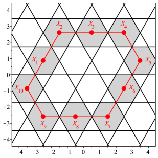
Figure 8: The centers points $p_{k,\ell}$ in the level $c=3.$

Proof.

Since $V_{k,\ell}$ depends on the signs of $2k+1,$ $2\ell+1$ and $k+\ell+1,$ we are going to consider the different cases.

1. Assume that $k<0$, $l\geq 0$ and $k+\ell+1\leq 0.$ From (5) we have that $V_{k,\ell}=\max\left(-2k-1,2\ell+1,-2k-2\ell-3\right),$ and from the inequalities $(2\ell+1)-(-2k-1)\leq 0$ and $(-2k-2\ell-3)-(-2k-1)<0$ we get that $V_{k,\ell}=-2k-1=c.$ Hence $c$ is odd, $k=-(1+c)/{2}$, $0\leq\ell\leq-k-1={(c-1)}/{2},$ and the points $p_{k,l}$ can be written as $p_{k,l}=\left(-c+\ell+{1}/{2},\sqrt{3}\left(\ell+{1}/{2}\right)\right)$ with $0\leq\ell\leq{(c-1)}/{2}.$ Hence, every $p_{k,l}$ lies on the straight line $y=\sqrt{3}(x+c)$ and that there are ${(c+1)}/{2}$ such points.

2. Assume that $k<0$, $l\geq 0$ and $k+\ell+1>0.$ Then, proceeding analogously to the previous case we get $V_{k,\ell}=2\ell+1=c.$ Hence $c$ is odd, $\ell={(c-1)}/{2}$ and ${-(c+1)}/{2}<k<0.$ We get the points $p_{k,l}=\left(2k+{(c+2)}/{2},{\sqrt{3}c}/{2}\right)$ with ${(1-c)}/{2}\leq k\leq-1.$ These points lie on the straight line $y={\sqrt{3}c}/{2}$ and there are ${(c-1)}/{2}$ such points.

3. Assume that $k\geq 0$ and $\ell\geq 0.$ Then $V_{k,\ell}=2k+2\ell+1=c>0.$ Hence $c$ is odd, $k={(c-1-2\ell)}/{2}$ and $0\leq\ell\leq{(c-1)}/{2}.$ We get the points $p_{k,l}=\left(c-\ell+{1}/{2},\sqrt{3}\left(\ell+{1}/{2}\right)\right)$ with $0\leq\ell\leq{(c-1)}/{2}.$ These points lie on $y=\sqrt{3}(-x+1+c)$ and there are ${(c+1)}/{2}$ such points.

4. Assume that $\ell<0,$ $k\geq 0$ and $k+\ell+1\geq 0.$ Then $V_{k,\ell}=2k+1=c.$ Hence $c$ is odd, $k={(c-1)}/{2}$ and ${-(c+1)}/{2}\leq\ell<0.$ We obtain the points $p_{k,l}=\left(c+\ell+{1}/{2},\sqrt{3}\left(\ell+{1}/{2}\right)\right)$ with ${-(c+1)}/2\leq\ell\leq-1,$ which lie on $y=\sqrt{3}(x-c)$ and there are ${(c+1)}/{2}$ such points.

5. Assume that $\ell<0,$ $k\geq 0$ and $k+\ell+1<0.$ Then $V_{k,\ell}=-2\ell-1=c.$ Hence $c$ is odd, $\ell={-(c+1)}/{2}$ and $0\leq k<{(c-1)}/{2}.$ We get the points $p_{k,l}=\left(2k+{(2-c)}/{2},-{\sqrt{3}c}/{2}\right)$ with $0\leq k\leq{(c-3)}/{2},$ which lie on $y=-{\sqrt{3}c}/{2}$ and there are ${(c-1)}/{2}$ such points.

6. Assume $k<0$ and $\ell<0.$ Then $k+\ell+1<0$ and $V_{k,\ell}=-2k-2\ell-3=c.$ Hence $c$ is odd, $k=-\ell-{(c+3)}/{2}$ with $-{(c+3)}/{2}<\ell<0.$ We get the points $p_{k,l}=\left(-c-\ell-{3}/{2},\sqrt{3}\left(\ell+{1}/{2}\right)\right)$ with $-{(c+1)}/{2}\leq\ell\leq-1,$ which lie on $y=-\sqrt{3}(x+c+1)$ and there are ${(c+1)}/{2}$ such points.

The Lemma follows from the above case-by-case study.    

Consider an odd energy level $V_{k,\ell}=c$; we will label the center points $p_{k,\ell}$ analogously as in the case $\alpha={\pi}/{2}$: we denote by $X_{1}$ the point on the corresponding irregular hexagon defined by the lines in the above lemma, which belongs to $H_{+}$ and its first component is the smallest one; that is, $X_{1}=(-c+{1}/{2},{\sqrt{3}}/{2}).$ After we denote by $X_{2},X_{3},\ldots X_{3c+1}$ the consecutive points on the hexagon turning clockwise (see Figure 8 for instance). The set of center points in such a level set is invariant under the action of $F$ and its dynamics is given in the next result:

Proposition 16.

Assume $m=k+\ell+1$. Fixed $V_{k,\ell}=c$ an odd number, consider the points $X_{1},X_{2},\ldots,X_{3c+1}$ introduced above. Then

1. For all $i=1,2,\ldots,3c+1$ , $F(X_{i})=X_{j}$ with $j\equiv i+c\text{ mod }(3c+1).$

2. The set $\{X_{1},X_{2},\ldots,X_{3c+1}\}$ is a periodic orbit of period $3c+1.$

Proof.

To prove statement $(a)$ we are going to consider the points that are on each of the six sides of the irregular hexagon delimited by the straight lines in Lemma 15.

• Consider the points $X_{1},X_{2},\ldots,X_{{(c+1)}/{2}}$ which lie on $y=\sqrt{3}(x+c).$ The map $F_{+}$ sends this straight line to $y=\sqrt{3}(-x+1+c)$ and

  $$F(X_{1})=F_{+}\left(-c+{1}/{2},{\sqrt{3}}/{2}\right)=\left({(c+2)}/{2},{\sqrt{3}c}/{2}\right)=X_{c+1}.$$

  Since the distance between two consecutive points is constant and $F_{+}$ is an isometry we get that $X_{2},X_{3},\ldots,X_{{(c+1)}/{2}}$ are mapped to $X_{c+2},X_{c+3},\ldots,X_{{(3c+1)}/{2}}$ respectively. In particular

  $$F(X_{i})=X_{i+c}$$ (8)

  for all $i=1,2,\ldots,X_{{(c+1)}/{2}}.$

• Now consider $X_{{(c+1)}/{2}},X_{{(c+3)}/{2}},\ldots,X_{c+1}$ which lie on $y={\sqrt{3}c}/{2}.$ $F_{+}$ sends $y={\sqrt{3}c}/{2}$ to the straight line $y=\sqrt{3}(x-c)$ and we already check that $X_{{(c+1)}/{2}}$ is mapped to $X_{{(3c+1)}/{2}}.$ Being $F_{+}$ an isometry we get that $X_{{(c+3)}/{2}},\ldots,X_{c+1}$ are mapped to $X_{{(3c+3)}/{2}},\ldots,X_{2c+1}$ respectively. Finally, equation (8) also holds for every $i={(c+1)}/{2},\ldots,c+1.$

• Following the same argument it is seen that $X_{c+1},X_{c+2},\ldots,X_{{(3c+1)}/{2}}$ are mapped to $X_{2c+1},X_{2c+2},\ldots,X_{{(5c+1)}/{2}}$ respectively.

• The points $X_{{(3c+3)}/{2}},\ldots,X_{2c+1}$ lie on $y=\sqrt{3}(x-c)$ and on $H_{-}.$ Then we have to take into account $F_{-}$ which maps $y=\sqrt{3}(x-c)$ to $y=-\sqrt{3}(x+c+1)$ and

  $$F(X_{{(3c+3)}/{2}})=F_{-}\left(c-{1}/{2},-{\sqrt{3}}{2}\right)=\left({-(c+2)}/{2},-{\sqrt{3}c}/{2}\right)=X_{{(5c+3)}/{2}}.$$

  Hence $F_{-}$ sends $X_{{(3c+5)}/{2}},\ldots,X_{2c+1}$ to $X_{{(5c+5)}/{2}},\ldots,X_{3c+1}$ respectively and (8) holds for every $i={(3c+3)}/{2},{(3c+5)}/{2},\ldots,2c+1.$

• Now consider the points of the irregular hexagon which lie on the straight line $y=-{\sqrt{3}c}/{2},$ that is, $X_{2c+1},\ldots,X_{{(5c+3)}/{2}}.$ The map $F_{-}$ sends $y=-{\sqrt{3}c}/{2}$ to $y=\sqrt{3}(x+c)$ and we verify that $X_{2c+1}$ is sent to $X_{3c+1}.$ Then $X_{2c+2},\ldots,X_{\frac{5c+3}{2}}$ are sent to $X_{1},\ldots,X_{{(c+1)}/{2}}.$ So $F(X_{i})=X_{j}$ with $j\equiv i+c\text{ mod }(3c+1)$ for $i=2c+1,\ldots,{(5c+3)}/{2}.$

• Finally, the points $X_{{(5c+5)}/{2}},\ldots,X_{3c+1}$ are on $H_{-}$ and also lie on $y=-\sqrt{3}(x+c+1)$. The map $F_{-}$ sends this straight line to $y={\sqrt{3}c}/{2}$ and since we already know that that $F_{-}(X_{{(5c+5)}/{2}})=X_{{(c+1)}/{2}}$ we get that $X_{{(5c+5)}/{2}},\ldots,X_{3c+1}$ are sent to $X_{{(c+3)}/{2}},\ldots,X_{c}$ respectively. Again $F(X_{i})=X_{j}$ with $j\equiv i+c\text{ mod }(3c+1)$ for every $i={(5c+5)}/{2},\ldots,X_{3c+1}$.

In order to prove $(b)$ we proceed as in the proof of Proposition 6. We use that the map $F$ restricted to $\{X_{1},X_{2},\ldots,X_{3c+1}\}$ is conjugated to $h:{\mathbb{Z}}_{3c+1}\longrightarrow{\mathbb{Z}}_{3c+1}$ defined by $h(i)=i+c.$ Then

$$F^{p}(X_{i})=X_{i}\Leftrightarrow h^{p}(i)=i\Leftrightarrow i+cp\equiv i\,\,\text{mod}\,\,(3c+1)\Leftrightarrow\exists n\in{\mathbb{N}}:cp=n(3c+1).$$

This implies that $p$ must be a multiple of $3c+1,$ and since $p\leq 3c+1$ we get that the minimal period is $p=3c+1$ as we wanted to see.    

4.2.2 Dynamics on the triangular tiles. The cases $m=k+\ell$ and $m=k+\ell+2$

For the triangular tiles, a result analogous to Lemma 15 is the following. We omit all the details.

Lemma 17.

1. Let $m=k+\ell$ and the points $q_{k,\ell}=\left(2k+\ell+{1}/{2},\sqrt{3}(\ell+{1}/{6})\right).$ Then

   1. $V(q_{k,\ell})=c$ is an even number.

   2. The set $\{q_{k,\ell}:V(q_{k,\ell})=c\}$ has $3c+1$ elements. In particular there are $3c+1$ triangles $T_{k,\ell,k+\ell}$ in this energy level.

   3. The points $q_{k,\ell}:V(q_{k,\ell})=c$ lie in the irregular hexagon determined by the intersection of the six straight lines $y=\sqrt{3}(x+c-{1}/{3}),y={\sqrt{3}}(3c+1)/6,y=-\sqrt{3}(x-c-{2}/{3}),y=\sqrt{3}(x-c-{1}/{3}),y=-{\sqrt{3}}(3c-1)/6$ and $y=-\sqrt{3}(x+c+{4}/{3}).$

2. Let $m=k+\ell+2$ and the points $r_{k,\ell}=\left(2k+\ell+{5}/{2},\sqrt{3}(\ell+{5}/{6})\right).$ Then

   1. $V(r_{k,\ell})=c$ is an even number.

   2. The set $\{r_{k,\ell}:V(r_{k,\ell})=c\}$ has $3c+1$ elements. In particular there are $3c+1$ triangles $T_{k,\ell,k+\ell}$ in this energy level.

   3. The points $r_{k,\ell}:V(r_{k,\ell})=c$ lie in the irregular hexagon determined by the intersection of the six straight lines $y=\sqrt{3}(x-c+{1}/{3}),y={\sqrt{3}}(3c-1)/6,y=-\sqrt{3}(x+c+{4}/{3}),y=\sqrt{3}(x-c+{1}/{3}),y=-{\sqrt{3}}(3c+1)/6$ and $y=-\sqrt{3}(x+c-{4}/{3}).$

   

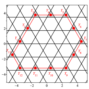
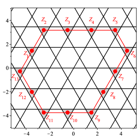
Figure 9: Position of the centers $q_{k,\ell}$ and $r_{k,\ell}$ in the level $c=4.$

For a fixed even number $c\geq 2$ consider $\{q_{k,\ell}:V(q_{k,\ell})=c\}$ (resp. $\{r_{k,\ell}:V(r_{k,\ell})=c\}$). We denote by $Y_{1}$ (resp. $Z_{1}$) the point $q_{k,\ell}$ (resp. $r_{k,\ell}$) in the corresponding irregular hexagon defined by the lines in the above lemma, which belongs to $H_{+}$ and its first component is the smallest one, that is $Y_{1}=\left(-c+{1}/{2},{\sqrt{3}}/{6}\right)$ (resp. $Z_{1}=\left(-c+{1}/{2},{5\sqrt{3}}/{6}\right)$). We denote by $Y_{2},Y_{3},\ldots,Y_{3c+1}$ (resp. $Z_{2},Z_{3},\ldots,Z_{3c+1}$) the consecutive points on the corresponding hexagon turning clockwise. See Figure 9 where the center points of the energy level $c=4$ are shown.

Proposition 18.

Consider a fixed even energy level $V_{k,\ell}=c$ and the points $Y_{1},Y_{2},\ldots,Y_{3c+1}$ and $Z_{1},Z_{2},\ldots,Z_{3c+1}$ defined above. Then

1. For all $i=1,2,\ldots,3c+1,$ $F(Y_{i})=Y_{j}$ with $j\equiv i+c\text{ mod }(3c+1)$ and $F(Z_{i})=Z_{j}$ with $j\equiv i+c\text{ mod }(3c+1).$

2. The set $\{Y_{1},Y_{2},\ldots,Y_{3c+1}\}$ is a periodic orbit of period $3c+1$ and the set $Z_{1},Z_{2},\ldots,Z_{3c+1}$ also is a periodic orbit of period $3c+1.$

The proof follows exactly by the same arguments involved in the proofs of Lemma 5 and Proposition 6. The next corollary simply consists of gluing (in a suitable way) the two sets given in the previous proposition, to form a single necklace with $6c+2$ triangular beads.

Corollary 19.

Consider a fixed even energy level $V_{k,\ell}=c$ and denote the set of $6c+2$ ordered points $Y_{1},Z_{1},Y_{2},Z_{2}\ldots,Y_{3c+1},Z_{3c+1},$ that we will denote $W_{i},i=1,2,\ldots,6c+2.$ Then for all $i=1,2,\ldots,6c+2,$ $F(W_{i})=W_{j}$ with $j\equiv i+2c\text{ mod }(6c+2).$

Proof of item $(i)$ of Theorem B.

Following the spirit of Definition 7, we can introduce the concept of itinerary map for the centers $p_{k,\ell}$, $r_{k,\ell}$ and $q_{k,\ell}$ in an analogous way. Then, the proof is exactly the same proof as for item $(i)$ of Theorem A. It is based on the fact that all the points in the same tile have the same itineraries of arbitrary length (a result analogous to Lemma 9) and also on Lemma 3.    

Proof of item $(ii)$ of Theorem B.

We start proving that $V=V_{3\pi/2}$ is a first integral. As in the proof of item $(ii)$ of Theorem A, we notice that since the tiles are completely contained in $H_{+}\setminus\{y=0\}$ or $H_{-}$ and the maps $F_{\pm}$ are rotations, then $F$ sends tiles to tiles. Remember that by its definition $V$ is constant on each tile, and in particular takes the value attained at the center point. The result follows now from the fact that in each level set, the set of centers is invariant, see Propositions 16 and 18.

Similarly that in the proof of Theorem A we consider the tile $T_{k,\ell,m}$. We know that all the points in the tile have the same itinerary than its center which, by Propositions 16, 18 and Corollary 19 give the discrete dynamical systems generated by the functions $h$ given in the statement of Theorem B between the corresponding ${\mathbb{Z}}_{M}.$ Moreover, we know that the centers are periodic with period $3c+1.$ Hence, if $I$ is the itinerary map associated with the center point, that is $I=\left.F^{3c+1}\right|_{T_{k,\ell,m}},$ we have that $I(T_{k,\ell,m})=T_{k,\ell,m}$. Writing $F(x,y)=A\cdot\left(x-\operatorname{sign}(y),y\right)^{t}$ where $A=R_{{2\pi}/{3}}$, we have $I=A^{3c+1}+v=A+v$ for a certain $v\in{\mathbb{R}}^{2},$ $v\neq 0,$ which implies that $I$ is a rotation with a unique fixed point, hence it is the center point. Furthermore $I^{3}=\operatorname{Id}$ because $I^{3}=A^{3}+(A^{2}+A+\operatorname{Id})v=\operatorname{Id},$ since $A^{2}+A+\operatorname{Id}=0.$ In summary, $I$ is a rotation of angle $\alpha={2\pi}/{3}$ which implies that the points $(x,y)\in T_{k,\ell,m}$ which are not centers are 3-periodic for $F^{3c+1}$ and consequently, they are $(9c+3)$-periodic.    

4.3 Proof of item $(iii)$ of Theorem B: dynamics in the non zero-free set

From the previous results, we know that the non zero-free set $\mathcal{F}$ is formed by the borders of the tiles, both hexagons and triangles.

Consider an energy level $c\in\mathbb{N}_{0}$. Assume that $c$ is an odd number, then the level set $\{V=c\}$ is formed by $3c+1$ hexagonal tiles, whose centers $X_{1},X_{2},\ldots,X_{3c+1}$ form a periodic orbit. Denoting by $H_{i}$ the closure of this hexagon we also know that $H_{1}$ and $H_{2c-1}$ intersect $y=0$ at the bottom edge while $H_{2c}$ and $H_{3c+1}$ intersect $y=0$ at the top edge. When $c$ is even, we have the points $Y_{1},Y_{2},\ldots,Y_{3c+1}$ (respectively, $Z_{1},Z_{2},\ldots,Z_{3c+1}$). Each $Y_{i}$ (resp. $Z_{i}$) is the center of an upward (resp. downward) facing triangle; its closure intersects $y=0$ only when $i=1$ and $i={(3c+2)}/{2}$ (resp. $i={(3c+2)}/{2}$ and $i=3c+1$), see Figure 10.

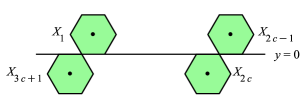
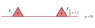
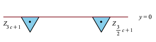
Figure 10: Position of the tiles which intersect $y=0.$

We are going to call perfect triangles the ones corresponding to $Y_{1},Y_{2},\ldots,Y_{3c+1}.$ As for perfect squares, we will prove that these figures will evolve avoiding the discontinuity of $F.$ They are positioned as the Figure 11 shows, the perfect triangles being the red ones, which are precisely the ones pointing upwards. The blue ones correspond to $Z_{1},Z_{2},\ldots,Z_{3c+1}.$

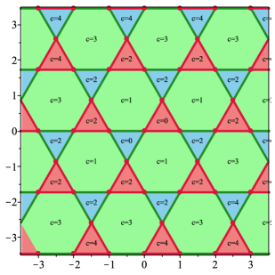
Figure 11: Position of the perfect triangles in red. The borders and the vertices are highlighted with the color of the tile having the same itinerary map. The level set $\{V=c\}$ is indicated in each tile.

Proof of item $(iii)$ of Theorem B.

First, we observe that the borders of the perfect triangles (including the vertices) have the same period as the interior points which are not centers. Indeed, set an even number $c\in\mathbb{N}_{0}$ and denote by $T_{i}$ the closed triangle (i.e. including the boundary with vertices) which contain the point $Y_{i}$. For $i\neq 1,{3c}/{2}+1,$ the triangle $T_{i}$ does not intersect $y=0,$ hence $F(T_{i})=T_{i+c}.$ For $i=1$ or $i={3c}/{2}+1,$ $F(T_{i})=F_{+}(T_{i})$ which also is $T_{i+c}.$ Therefore, by continuity, the points in the boundary of $T_{i}$ are periodic with period $3(3c+1)=9c+3,$ as for the points in the interior of $T_{i}.$

Now take $c$ odd and let $H_{i}$ be the closed hexagon which contains $X_{i}$ in its interior. Looking at Figure 11 we see that $H_{i}$ has three edges which also are edges of a perfect triangle; if we call these edges the perfect edges, we consider $\widetilde{H}_{i}=H_{i}\setminus\text{perfect edges}.$ (the motivation for this name is similar that the ones of perfect triangles, or squares, and will be apparent later). Then, $\widetilde{H}_{i}$ contains three alternate edges, say $l_{1},l_{2},l_{3}$, such that the slopes of the straight lines which contain them are $\sqrt{3},-\sqrt{3}$ and $0$ respectively. Observe that $l_{3}$ is always at the bottom of the hexagon, hence $\widetilde{H}_{i}$ is always fully contained in $H_{+}$ and $H_{-}$, and therefore $F(\widetilde{H}_{i})=F_{+}(\widetilde{H}_{i})$ or $F(\widetilde{H}_{i})=F_{-}(\widetilde{H}_{i}).$ In any case the three edges included in $F(\widetilde{H}_{i})$ are three alternate edges with the edge of slope $0$ in the bottom of the hexagon $F(\widetilde{H}_{i}).$ That is, $F(\widetilde{H}_{i})=\widetilde{H}_{i+c}$ for all $i=1,2,\ldots,3c+1.$ As in the previous case, by continuity, the points in the boundary of $\widetilde{H}_{i}$ are periodic with period $9c+3,$ as for the points in the interior of $H_{i}.$ Hence we have proved that all the points in the edges of the hexagons are periodic points.

It remains to consider the edges of the triangles which are not perfect. But, as can be seen in Figure 11, all these edges are also the edges of the contiguous hexagons, which we have already proved that all of them are periodic. Observe also that all the vertices belong to perfect triangles.    

4.4 Proof of item $(iv)$ of Theorem B

As in the case $\alpha=\pi/2,$ the proof follows by replacing the value of $V$ by $2n$ or $2n+1,$ for $n\in{\mathbb{N}}_{0},$ in the results of the previous items. We re-obtain the results of [10].

5 Proof of Theorem C

5.1 Preliminaries

As in the case studied in the previous section, for each tile $T_{k,\ell,m},$ the values $k,\ell,m$ are not independent. Here, either $m=k+\ell-1$ or $m=k+\ell$ or $m=k+\ell+1.$

Lemma 20.

Let $T_{k,\ell,m}$ be one tile of $\mathcal{U}_{\pi/3}=\mathcal{U}$.

1. If $m=k+\ell$ then $T_{k,\ell,m}$ is a hexagon whose center is $p_{k,\ell}=\left(2k+\ell+{1}/{2},\sqrt{3}\ell+{\sqrt{3}}/{2}\right).$

2. If $m=k+\ell-1$ or $m=k+\ell+1$, then $T_{k,\ell,m}$ is a triangle whose center is either $q_{k,\ell}=\left(2k+\ell-{1}/{2},\sqrt{3}\ell+{\sqrt{3}}/{6}\right)$ or $r_{k,\ell}=\left(2k+\ell+{3}/{2},\sqrt{3}\ell+{5\sqrt{3}}/{6}\right),$ respectively.

5.2 Proof of items $(i)$ and $(ii)$ of Theorem C: dynamics on the zero-free set

These results can be proved by the same arguments that we have used in the proofs of Theorems A and B, in Sections 3 and 4. Although we will not give all the details of their proofs, we want to highlight the main features and results that allow to give the dynamics in this case.

Consider an even number $c$. Then, by Lemma 20, the tiles on the level set $V=c$ are hexagons whose centers are some of the points $p_{k,\ell}$ for some $k,\ell.$ It can be proved that there are $3c+2$ centers in this level. This centers lie in certain hexagons. We denote them by $\{X_{1},X_{2},\ldots,X_{3c+2}\}$ labeling them as in the case $\alpha={2\pi}/{3},$ see the Figure 12.

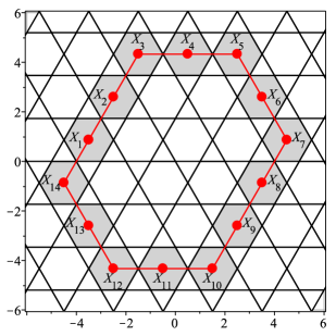
Figure 12: Position of the centers in the level $c=4.$ Observe that the points do not belong to the same orbit. In this case there are two different orbits. The lines linking the centers are plotted because their expressions play a role in order to obtain the expression of the first integrals $V$, as explained in Section 6.

In this case $F$ restricted to $\{X_{1},X_{2},\ldots,X_{3c+2}\}$ is conjugated to

$$h:{\mathbb{Z}}_{3c+2}\longrightarrow{\mathbb{Z}}_{3c+2}\mbox{ where }h(i)=i+{c}/{2}.$$ (9)

From this equality, and using that $3c\equiv-2$ mod $3c+2$, one easily gets that when ${c}/{2}$ is even then the minimal period is $3{c}/{2}+1$, and that when ${c}/{2}$ is odd, then the minimal period is $3c+2$. In the first case we get two periodic orbits $\{X_{1},X_{3},\ldots,X_{3c+1}\}$ and $\{X_{2},X_{4},\ldots,X_{3c+2}\}$ while in the second one all the points $X_{i}$, $i=1,2,\ldots,3c+1$ belong to the same periodic orbit.

To study the periodicity of the points in the hexagonal tile different from its center, for each $X_{j}$ we consider its itinerary map $I_{j}.$

• When ${c}/{2}$ is even, $I_{j}$ has the form $I_{j}=A^{3{c}/{2}+1}+v$ (where $v=X_{j}-A^{3{c}/{2}+1}X_{j}$) and $3{c}/{2}+1=3\cdot 2n+1=6n+1$ for some $n\in{\mathbb{N}}_{0}.$ Hence, since $A^{6}=\operatorname{Id},$ it holds that $I_{j}=A+v.$ Therefore $I_{j}$ restricted to the hexagon which contains $X_{j},$ is a rotation of angle ${\pi}/{3}$ centered at $X_{j}$ and every point in the hexagon is a 6-periodic point for $I_{j}.$ It implies that these points are $6(3{c}/{2}+1)=9c+6$ periodic points for $F.$

• When ${c}/{2}$ is odd, $I_{j}=A^{3c+2}+v$ and $3c+2=3\cdot 2(2n+1)+2=6(2n+1)+2$ for some $n\in{\mathbb{N}}_{0}.$ Thus $I_{j}=A^{2}+v,$ using again that $A^{6}=\operatorname{Id}.$ This implies that every point in the hexagon is a $3(3c+2)=9c+6$ periodic point for $F.$

Now let $c$ be an odd number. Then the tiles in $\{V=c\}$ are triangles whose centers are either the points $q_{k,\ell}$ or the points $r_{k,\ell}$ introduced in Lemma 20, for some $k,\ell\in{\mathbb{Z}}$. The points $q_{k,\ell}$ lie in some lines that define a hexagon, as do the points $r_{k,\ell}.$ But now all these centers belong to the same periodic orbit. To prove this, as usual, we label these points in a clockwise direction, as Figure 13 shows for the case $c=3$: the red points are the points $q_{k,\ell}\in\{V=3\}$ while the blue ones are $r_{k,\ell}\in\{V=3\}.$

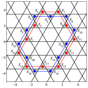
Figure 13: Position of the centers in the level $c=3.$ Observe that all the points belong to the same orbit. As shown in Section 6, the lines joining the centers play a role in the determination of the first integral $V$ and do not represent two different orbits.

With this labeling it can be proved that $F(X_{i})=X_{j}$ with $j\equiv i+c$ (mod $6c+4$) which implies that the minimal period is $p=6c+4.$ To see the periodicity of the points in the triangles different from its center we consider the itinerary function of the center $X_{j}$ which has the form $I_{j}=A^{4}+v.$ Then $I_{j}^{3}=A^{12}+(A^{4}+A^{2}+\operatorname{Id})v=\operatorname{Id}.$ Arguing as before we get that each point in the triangle different from its center is a $3(6c+4)=18c+12$ periodic point.

5.3 Proof of item (iii) of Theorem C: dynamics on the non zero-free set

In this case, the dynamics of the points on the edges and vertices of the tiles is more complicated than the ones found in the cases $\alpha={\pi}/{2}$ and $\alpha={2\pi}/{3},$ so we are going to give the details.

5.3.1 Perfect edges and vertices

We begin by considering the levels $c=4k,$ $k\in{\mathbb{N}}.$ We already know that in these levels there are $3c+2=12k+2$ centers, $X_{1},X_{2},\ldots,X_{12k+2}$ and $F(X_{i})=X_{j}$ where $j=i+2k$ mod $(12k+2).$ Also $X_{1},X_{3},\ldots,X_{12k+1}$ form a periodic orbit of period $6k+1$, as does $X_{2},X_{4},\ldots X_{12k+2}.$ Let $H_{j}$ be the hexagon such that $X_{j}\in H_{j}$ including its boundary (hence also its vertices). Then the hexagons that meet $y=0$ are $H_{1},H_{6k+1}$ (its bottom edge is contained in $y=0$) and $H_{6k+2},H_{12k+2}$ (its top edge is contained in $y=0$). See Figure 14.

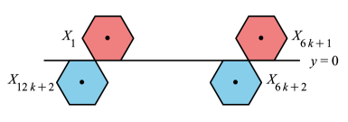
Figure 14: Position of the hexagonal tiles of a level $c=4k$ which intersect $y=0.$ The red ones belong to the set of perfect hexagons.

Clearly for all $j=1,2,\ldots,6k+1$, $F(H_{j})=F_{+}(H_{j})=H_{j+2k}$. while for $j=6k+3,6k+4,\ldots,12k+1$ also $F(H_{j})=F_{-}(H_{j})=H_{j+2k\mbox{ mod }(12k+2)}.$ But the hexagons $H_{6k+2},H_{12k+2}$ do not satisfy this property because on the top edge of these hexagons $F=F^{+}$. Then we easily get:

Lemma 21.

Assume that $c=4k$ and consider the (closed) hexagons $H_{1},H_{3},\ldots,H_{12k+1}.$ Then for all $j=1,3,\ldots,12k+1$ every point in $H_{j}$ different from its center is periodic of period $36k+6.$

Proof.

For $j=1,3,\ldots,12k+1$, the hexagons satisfy $F(H_{j})=H_{j+2k\mbox{ mod }(12k+2)},$ hence it is easy to observe that their images are never the hexagons $H_{6k+2}$ and $H_{12k+2}$. Then, by continuity, every point on the boundary of $H_{j}$ has the same periodicity as the points inside the hexagon (except the center). In particular, $H_{1},H_{3},\ldots,H_{12k+1}$ form an invariant set.    

As in the above sections we call $H_{1},H_{3},\ldots,H_{12k+1}$ perfect hexagons and their edges and vertices behave as the corresponding interior points, apart from the centers, that is they are $(36k+6)-$ periodic. Also we will call non-perfect edges or vertices those which do not collide with a perfect hexagon.

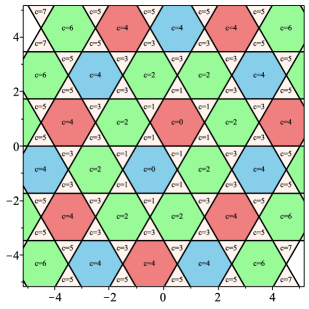
Figure 15: Position of the perfect hexagons in red. The level $\{V=c\}$ is indicated in each set.

5.3.2 Non-perfect edges

We continue the study considering the even levels of the form $c=4k+2$. We know that in these level sets there are $3c+2=12k+8$ centers and that all of them belong to the same periodic orbit. The hexagons which meet $y=0$ are $H_{1},H_{6k+4},H_{6k+5}$ and $H_{12k+8}$, see Figure 16.

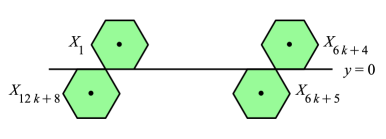
Figure 16: Position of the hexagonal tiles of a level $c=4k+2$, which intersect $y=0.$

We are going to follow the dynamics of the interior of the bottom edge of $H_{1},$ that we will denote as $\mathcal{L}$ (for simplicity we will use the term edge although the two boundary points are not included). This dynamics is, by far, the most complex of those we have studied in this paper. Since the argument is long, we first briefly summarize it: we will show that every point in $\mathcal{L}$ is $(108k+72)$-periodic. The edge is rigidly mapped by by iterating $F$ into the edges of the hexagons in the level $4k+2$, but also into the edges of the triangles in the levels $4k+1$ and $4k+3$.

Indeed, after the first iteration, $F(\mathcal{L})$ is the edge of $H_{2k+2}$ obtained after rotating $\mathcal{L}$ an angle equal to ${\pi}/{3}$, because $F(X_{1})=X_{2k+2}$ (remember that from (9), $F(X_{i})=X_{i+2k+1\mbox{ mod }(12k+8)}.)$ We continue iterating until we find the hexagon $H_{6k+5}.$ To compute how many iterations we need for $X_{1}$ to reach $X_{6k+5}$ we ask for the minimal positive number $p$ such that $F^{p}(X_{1})=X_{6k+5}.$ That is, $F^{p}(X_{1})=X_{6k+5},$ or equivalently, $1+p(2k+1)\equiv 6k+5\mbox{ mod }(12k+8).$ Thus,

$$p\equiv(2k+1)^{-1}(6k+4)=(6k+1)(6k+4)=36k^{2}+30k+4\equiv 6k+4\mbox{ mod }(12k+8).$$

That is $F^{6k+4}(X_{1})=X_{6k+5}.$ Now $F^{6k+4}(\mathcal{L})$ is the edge of $H_{6k+5}$ after rotating $\mathcal{L}$ an angle equal to $\frac{4\pi}{3}.$ Hence we follow iterating until we arrive to $X_{12k+8},$ that is, three iterates more: $F^{3}(X_{6k+5})=X_{12k+8}.$ This implies that $F^{6k+7}(\mathcal{L})$ is the edge of $H_{12k+8}$ obtained after rotating $\mathcal{L}$ an angle equal to ${\pi}/{3}.$ Now we ask for the minimal $p$ such that $F^{p}(X_{12k+8})=X_{6k+5}.$ The computation gives that $p=12k+5.$ Hence we can write

$$X_{1}\overset{F^{6k+4}}{\longrightarrow}X_{6k+5}\overset{F^{3}}{\longrightarrow}X_{12k+8}\overset{F^{12k+5}}{\longrightarrow}X_{6k+5}\overset{F^{3}}{\longrightarrow}X_{12k+8},$$

and following the edge $\mathcal{L}$ we have that after $18k+15$ iterates the initial edge $\mathcal{L}$ of $H_{1}$ is the top edge of $H_{12k+8},$ which is the bottom edge of the triangle $T_{1}$ in the level $4k+3$.

Next, we follow the orbit of the centers of the triangles in the level $c=4k+3$. Let $Y_{1},Y_{2},\ldots,Y_{24k+22}$ be the centers of the triangles $T_{1},T_{2},\ldots,T_{24k+22}$. All of them form a unique periodic orbit and $F(Y_{i})=Y_{j}$ where $j=i+4k+3$ mod $(24k+22)$, remember that in the triangles $F(Y_{i})=Y_{i+c\mbox{ mod }(6c+4)}$. The triangles with edges in the critical line are displayed in the Figure 17.

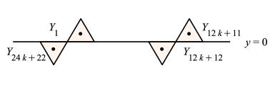
Figure 17: Position of the triangular tiles which intersect $y=0.$

Taking into account that $(4k+3)^{-1}=18k+15$ in ${\mathbb{Z}}_{24k+22}$ and solving the corresponding congruences we find that:

$$Y_{1}\overset{F^{6k+7}}{\longrightarrow}Y_{24k+22}\overset{F^{6k+4}}{\longrightarrow}Y_{12k+12}\overset{F^{18k+18}}{\longrightarrow}Y_{24k+22}\overset{F^{6k+4}}{\longrightarrow}X_{12k+12}.$$

Then we see that the bottom edge of $T_{1}$ is transformed into the top edge of $T_{12k+12}$ after $36k+33$ iterates. This one also is the bottom edge of the hexagon $H_{6k+4}$ in the level $c=4k+2,$ see again Figure 15, and also Figure 3.

Following the same procedure it can be seen that $F^{6k+1}(X_{6k+4})=X_{6k+5}$ and using the calculations made before we obtain

$$X_{6k+4}\overset{F^{6k+1}}{\longrightarrow}X_{6k+5}\overset{F^{3}}{\longrightarrow}X_{12k+8}\overset{F^{12k+5}}{\longrightarrow}X_{6k+5}.$$

Hence, the bottom edge of $H_{6k+4}$ is transformed into the top edge of $H_{6k+5}$ after $18k+9$ iterates.

The top edge of $H_{6k+5}$ is also the bottom edge of one triangle whose center belongs to the level set $4k+1.$ In this level set there are $24k+10$ centers of triangles, that we denote by $Z_{1},Z_{2},\ldots,Z_{24k+10},$ and we know that $F(Z_{i})=Z_{j}$ with $j=i+4k+1$ mod $(24k+10).$ We call $T_{1},T_{2},\ldots,T_{24k+10}$ these triangles. Specifically, the top edge of $H_{6k+5}$ is the bottom edge of $T_{12k+5}$, see Figures 15 and 18.

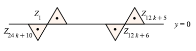
Figure 18: Position of some of the triangular the tiles which intersect $y=0.$

Using that in ${\mathbb{Z}}_{24k+10}$, $(4k+1)^{-1}=6k+1$ and solving the corresponding congruences we have that

$$Z_{12k+5}\overset{F^{6k+1}}{\longrightarrow}Z_{12k+6}\overset{F^{6k+4}}{\longrightarrow}Z_{24k+10}\overset{F^{18k+6}}{\longrightarrow}Z_{12k+6}\overset{F^{6k+4}}{\longrightarrow}Z_{24k+10}.$$

It follows that after $36k+15$ iterates, the bottom edge of $T_{12k+5}$ is transformed in the top edge of $T_{24k+10}.$

But this top edge of $T_{24k+10}$ is exactly the edge $\mathcal{L}$. Hence summing up the involved iterates we have that every point in $\mathcal{L}$ is a $108k+72$ periodic point. Also the same holds for all the points belonging to the $108k+72$ edges obtained iterating $\mathcal{L}.$ In other words, we get a periodic orbit of edges of period $108k+72$ and, of course, the points of $\mathcal{L}$ are mapped to themselves after these iterations.

5.3.3 Non-perfect vertices

And what about the vertices? As we will see in the proof of Theorem 22, we only need to prove the periodicity of the vertices in $y=0$. Observe that if such a vertex belongs to a perfect hexagon, then we already know that it is periodic with the same period as the interior points. If it is non-perfect, then either $(a)$ it is mapped to a vertex colliding from the top with a triangle of level $V=4k+1$ and a hexagon of level $V=4k+2$, both in $H_{+}$, as the solid-circle point in Figure 19; or (b) it collides from the top with a hexagon of level $V=4k+2$ and triangle of level $V=4k+3$, both in $H_{+}$, as the box-shaped point in Figure 19.

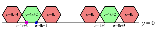
Figure 19: Position of the non-perfect vertices in $y=0$. If $H_{1}$ is the left non-perfect hexagon with level $V=4k+2$ then the vertex $V_{1}(H_{1})$ is the box-shaped point and the vertex $V_{6}(H_{1})$ is the solid-circle point. The perfect hexagons are the red ones.

To study the dynamics of the non-perfect vertices in $y=0$, we will use the following notation: given a hexagon $H$, we label its vertices as $V_{i}(H)$ with $i=1,\cdots,6$ starting from the left-bottom vertex and in clockwise sense, see Figure 20.

Figure 20: Labeling the vertices of a hexagon $H$

Let $H_{1}$ be the non-perfect hexagon at level $V=4k+2$ in $\mathcal{Q}_{1}$, whose intersection with $y=0$ is its bottom edge. Then:

$(a)$ We will follow the orbit of the point $V_{6}(H_{1})$ (the blue point in Figure 19) by using the results found in Section 5.3.2. In particular, we know that $F^{3}(H_{1})=H_{6k+4}$ , $F^{6k+1}(H_{6k+4})=H_{6k+5}$ , $F^{3}(H_{6k+5})=H_{12k+8}$ and $F^{6k+1}(H_{12k+8})=H_{1}.$ Therefore, we easily find

$$V_{6}(H_{1})\overset{F^{3}}{\longrightarrow}V_{3}(H_{6k+4})\overset{F^{6k+1}}{\longrightarrow}V_{4}(H_{6k+5})=V_{1}(H_{6k+4})\overset{F^{6k+1}}{\longrightarrow}$$

$$V_{2}(H_{6k+5})\overset{F^{3}}{\longrightarrow}V_{5}(H_{12k+8})\overset{F^{6k+1}}{\longrightarrow}V_{6}(H_{1}),$$

hence the point $V_{6}(H_{1})$ is $(18k+9)$-periodic.

(b) We will pursue the orbit of the point $V_{1}(H_{1})$ (the box-shaped point in Figure 19).

$$V_{1}(H_{1})\overset{F^{3}}{\longrightarrow}V_{4}(H_{6k+4})\overset{F^{6k+1}}{\longrightarrow}V_{5}(H_{6k+5})\overset{F^{3}}{\longrightarrow}V_{2}(H_{12k+8})\overset{F^{6k+1}}{\longrightarrow}V_{3}(H_{1})\overset{F^{3}}{\longrightarrow}$$

$$V_{6}(H_{6k+4})\overset{F^{6k+1}}{\longrightarrow}V_{1}(H_{6k+5})\overset{F^{3}}{\longrightarrow}V_{4}(H_{12k+8})=V_{1}(H_{1}),$$

hence the point $V_{1}(H_{1})$ is $(18k+15)$-periodic.

Now we have all the ingredients to prove the main result of this section, that clearly implies item $(iii)$ of Theorem C.

Theorem 22.

Every non zero-free point of $F$ is periodic. Furthermore:

1. If $(x,y)$ is a point in the edge of a perfect hexagon (which has energy level $V=4k$), then it is periodic with period $36k+6$.

2. If $(x,y)$ is a point in a non-perfect (open) edge of a tile then it is periodic with period $108k+72$ for some $k\in\mathbb{N}_{0}$.

3. If $(x,y)$ is a non-perfect vertex then it is periodic with period $18k+9$ or $18k+15$ for some $k\in\mathbb{N}_{0}$.

Observe that any non zero-free point belongs to one of the above cases.

Proof.

We already know that the set of the non zero-free points is formed by the edges and the vertices of the hexagons and triangles introduced before.

Consider the points in one edge. Then after a finite number of iterates this edge is transformed in one edge contained in $y=0.$ If this edge correspond to an edge of a perfect hexagon with center belonging to the level $4k,$ every point will be $6(6k+1)-$periodic. If not, it will be an edge of a polygon with center belonging to the level either $4k+1,4k+2$ or $4k+3.$ From the discussion above we know that every point will be $(108k+72)-$periodic.

With respect to the vertices, observe that since any vertex belongs to $\mathcal{F}$, after some iterates it will be mapped to a vertex point in $y=0$. Hence there are three possibilities: it is mapped to a perfect vertex of a perfect hexagon in $H_{+}$, which has energy level $V=4k$ (and in this case it is periodic of period $36k+6$); or it is mapped to a vertex colliding from the top with a triangle of level $V=4k+1$ and a hexagon of level $V=4k+2$ (and in this case it is periodic with period $18k+9$); or it is mapped to a vertex colliding from the top with a hexagon of level $V=4k+2$ and a triangle of level $V=4k+3.$ In this case it is periodic with period $18k+15.$    

The proof of item $(iv)$ is a straightforward consequence of all the previous results.

6 Obtaining the first integrals

We have intuited the expressions of the first integrals after several simulations. For completeness we present in detail a three-step constructive procedure that allows to obtain the first integrals of $F$ given in (3) corresponding to $\alpha=\pi/2.$ For the other two cases the line of argument is the same, and the details are analogous, and we only give some comments.

Step 1. By displaying some preimages of the critical line $LC_{-i}$ we realize that the zero-free set is formed by open tiles of a regular or uniform tessellation of ${\mathbb{R}}^{2}$. This fact is trivial in this case where $\alpha=\pi/2$ but, a priori, it was not so obvious in the cases $\alpha=2\pi/3$ and $\alpha=\pi/3$ studied in Sections 4 and 5. The normal form of $F$ given in (2) regularizes the tesselation.

Step 2. From preliminary numerical explorations we also realize that the centers of some tiles form an invariant set under the dynamics of $F.$ In the case $\alpha=\pi/2$ these centers were located in the lines $y=x+c$, $y=-x+c+1$, $y=x-c$ and $y=-x-c-1$ for a certain fixed value $c\in\mathbb{N}_{0}$, depending on the quadrant where the center points are located (see Lemma 4 and Figure 4, and see Lemmas 15 and 17 for the case $\alpha=2\pi/3$).

Step 3. Isolating the value in the expression of the lines linking the centers we obtain that $c=y-x$ for $(x,y)\in\mathcal{Q}_{1}$, $c=y+x-1$ for $(x,y)\in\mathcal{Q}_{2}$, $c=x-y$ for $(x,y)\in\mathcal{Q}_{3}$ and $c=-x-y-1$ for $(x,y)\in\mathcal{Q}_{4},$ where recall that $\mathcal{Q}_{j},j=1,2,3,4,$ are the four quadrants of ${\mathbb{R}}^{2}.$ From these expressions and taking into account that $c\in\mathbb{N}_{0}$ and that given a zero-free point $(x,y)$ the center point of its associated tile is $\left(\operatorname{E}(x)+{1}/{2},\operatorname{E}(y)+{1}/{2}\right)$, we arrive to the expression of the first integral $V_{\pi/2}(x,y)=\max\left(\left|\operatorname{E}(x)+\operatorname{E}(y)+1\right|-1,\left|\operatorname{E}(x)-\operatorname{E}(y)\right|\right).$

7 Final comments.

We have proved that for $\alpha\in\{\pi/3,\pi/2,2\pi/3\}$, the corresponding zero-free sets $\mathcal{U}$ are the union of a countable number of open sets (the tiles), hence the associated critical sets $\mathcal{F}=\mathbb{R}^{2}\setminus\mathcal{U}$ are closed sets. In consequence, for any point $(x,y)\in\mathbb{R}^{2}$, the distance $\mathrm{dist}\left((x,y),\mathcal{F}\right)$ is well defined. Since $\mathcal{F}$ is also invariant, we have:

Remark 23.

Any map (2) with $\alpha\in\{\pi/3,\pi/2,2\pi/3\}$ has the non-quantized continuous first integral $W(x,y)=\mathrm{dist}\left((x,y),\mathcal{F}\right)$.

We believe that the only pointwise periodic cases for the maps $F$ with $\alpha\in(0,2\pi)$, are the ones studied in this work as well the cases $\alpha\in\{4\pi/3,3\pi/2,5\pi/3\}$ (recall that we where motivated by the study of the maps $G$ in (1) with $|\rho|<2$, which are conjugated with the maps $F$ in (2) with $\alpha\in(0,\pi)$). In these later cases we have observed that the quantized first integrals given in this paper are also integrals of these maps. In particular: $V_{\pi/2}$, $V_{2\pi/3}$ and $V_{\pi/3}$ are first integrals of $F$ when $\alpha=3\pi/2,5\pi/3$ and $4\pi/3$ respectively. However notice that none of these last maps are conjugated to the maps considered in this work: for example, note that the maps $F$ with $\alpha\in\{4\pi/3,3\pi/2,5\pi/3\}$ do not have fixed points since the centers of the rotations are virtual.

The maps $F$ belong to the class of symmetric maps studied in the relevant paper [14]. We refer the reader to this reference to learn about the general properties of the maps $F$ with $\alpha$ a general value in $[0,2\pi)\setminus\{{\pi}/{3},\pi/{2},2\pi/{3},4\pi/3,3\pi/2,5\pi/3\}$. For instance, in that paper it is proved that for any $\alpha\neq\pm\pi$ being a rational multiple of $\pi$ there exists a sequence of open invariant nested necklaces, that tend to infinity, each one of them being similar to the level sets of our quantized first integrals, whose beads are polygons, and where the dynamics of $F$ is given by a product of two rotations. Remarkably, although the adherence of the union of all these invariant necklaces does not fill the full plane, it allows to prove that all orbits of $F$ are bounded.

Acknowledgements

We want to thank the anonymous reviewers for their comments that have allowed us to better contextualize the problem, improve our article and have provided us with very interesting references. The authors are supported by Ministry of Science and Innovation–State Research Agency of the Spanish Government through grants PID2019-104658GB-I00 (first and second authors), DPI2016-77407-P (AEI/FEDER, UE, third author) and MTM2017-86795-C3-1-P (fourth autor). The first, second and fourth authors are also supported by the grant 2017-SGR-1617 from AGAUR, Generalitat de Catalunya. The third author acknowledges the group’s research recognition 2017-SGR-388 from AGAUR, Generalitat de Catalunya.

References

- [1] V. Avrutin, L. Gardini, I. Sushko, F. Tramontana. Continuous and discontinuous piecewise-smooth one-dimensional maps. Invariant sets and bifurcation structures. World Scientific, Hackensack (NJ) 2019.
- [2] S. Banerjee, G.C. Verghese (eds). Nonlinear Phenomena in Power Electronics. IEEE Press, New York 2001.
- [3] M. di Bernardo, C.J. Budd, A.R. Champneys, P. Kowalczyk. Piecewise-Smooth Dynamical Systems: Theory and Applications. Springer, London 2008.
- [4] G.I. Bischi, L. Gardini, C. Mira. Maps with denominator. Part 1: some generic properties. Int. J. Bifurcation & Chaos 9 (1999), 119–153.
- [5] M. Boshernitzan, A. Goetz. A dichotomy for a two-parameter piecewise rotation. Ergod. Th. & Dynam. Sys. 23 (2003), 759–770.
- [6] B. Brogliato. Nonsmooth Mechanics: Models, Dynamics and Control. Springer-Verlag, New York 1999.
- [7] Y. C. Chang, S. S. Cheng. Complete periodicity analysis for a discontinuous recurrence equation. Int. J. Bifurcations and Chaos 23 (2013), 1330012 (34 pages).
- [8] Y. C. Chang, S. S. Cheng. Complete periodic behaviours of real and complex bang bang dynamical systems. J. Difference Equations and Appl. 20 (2014), 765–810.
- [9] Y. C. Chang, S. S. Cheng, Y. C. Yeh. Abundant periodic and aperiodic solutions of a discontinuous three-term recurrence relation. J. Difference Equations and Appl. 25 (2019), 1082–1106.
- [10] Y. C. Chang, G. Q. Wang, S. S. Cheng. Complete set of periodic solutions of a discontinuous recurrence equation. J. Difference Equations and Appl. 18 (2012), 1133–1162.
- [11] A. Cima, A. Gasull, V. Mañosa. Global periodicity and complete integrability of discrete dynamical systems. J. Difference Equations and Appl. 12 (2006), 697–716.
- [12] A. Cima, A. Gasull, V. Mañosa, F. Mañosas. Different approaches to the global periodicity problem. In Ll. Alsedà et al. eds. Difference Equations, Discrete Dynamical Systems and Applications (ICDEA 2012). Springer Proceedings in Mathematics & Statistics Vol. 180. pp. 85–106. Springer, Berlin 2016.
- [13] F. Dogru, S. Tabachnikov. Dual billiards. Math. Intelligencer 27 (2005), 18–25.
- [14] A. Goetz, A. Quas. Global properties of a family of piecewise isometries. Ergod. Th. & Dynam. Sys. 29 (2009), 545–568.
- [15] B. Grünbaum, G.C. Shephard. Tilings by regular polygons. Math. Mag. 50 (1977), 227–247.
- [16] B. Grünbaum, G.C. Shephard. Tilings and Patterns. W.H. Freeman and Co., New York 1987.
- [17] E. Gutkin, N. Simanyi. Dual polygonal billiards and necklace dynamics. Commun. Math. Phys. 143 (1992), 431–449.
- [18] C. Mira, L. Gardini, A. Barugola, J.C. Cathala. Chaotic Dynamics in Two-Dimensional Noninvertible Maps. World Scientific, Singapore 1996.
- [19] D. Montgomery. Pointwise periodic homeomorphisms Amer. J. Math. 59 (1937), 118–120.
- [20] J. Moser. Is the solar system stable? Math. Intelligencer 1 (1978), 65–71.
- [21] O. Neugebauer. The Exact Sciences in Antiquity. Dover, New York 1969.
- [22] D.J.W. Simpson, J.D. Meiss. Neimark-Sacker bifurcations in planar, piecewise-smooth, continuous maps. SIAM J. Appl. Dyn. Syst. 7 (2008), 795–824.
- [23] F. Vivaldi, A.V. Shaidenko Global stability of a class of discontinuous dual billiards. Commun. Math. Phys. 110 (1987), 625–640.
- [24] Z.T. Zhusubaliyev, E. Mosekilde. Bifurcations and Chaos in Piecewise-Smooth Dynamical Systems. World Scientific. Singapore 2003.