Unpredictable and Uniform RNG based on time of arrival using InGaAs Detectors

Abstract

Quantum random number generators are becoming mandatory in a demanding technology world of high performing learning algorithms and security guidelines. Our implementation based on principles of quantum mechanics enable us to achieve the required randomness. We have generated high-quality quantum random numbers from a weak coherent source at telecommunication wavelength. The entropy is based on time of arrival of quantum states within a predefined time interval. The detection of photons by the InGaAs single-photon detectors and high precision time measurement of 5 ps enables us to generate 16 random bits per arrival time which is the highest reported to date. We have presented the theoretical analysis and experimental verification of the random number generation methodology. The method eliminates the requirement of any randomness extractor to be applied thereby, leveraging the principles of quantum physics to generate random numbers. The output data rate is on an average of 2.4 Mbps. The raw quantum random numbers are compared with NIST prescribed Blum-Blum-Shub pseudo random number generator and an in-house built hardware random number generator from FPGA, on the ENT and NIST Platform.

I Introduction:

The importance of random numbers was realised much early in human society, its requirement was governed by the beliefs and socioeconomic structure. The methods of generating random numbers evolved with the development of science and technology. In the present era, random numbers play a significant role in statistical analysis, stochastic simulations, cyber security applications, gaming, cryptography, and many others. Random numbers can be generated by two approaches, a software approach termed as pseudo random number generator (PRNG) is based on mathematical algorithm and a hardware approach termed as true random number generator (TRNG) that can extract randomness from physical processes. In software approach, we cannot deny the possibility of backdoor, reapplication of seed generates same random numbers repeatedly and a weak entropy can substantially compromise the security system. These issues can be overcome by TRNG. However, if the physical process is classical in nature it employs causality behind complexity. A TRNG based on quantum physics is termed as quantum random number generator (QRNG). The probabilistic nature of quantum mechanics can be employed to generate true random numbers that are unpredictable, irreproducible, and unbiased. It generates random numbers as a result of measurement on a quantum system. The quality of quantum random numbers is strongly dependent on the properties or behavior of the quantum entity and the elimination of classical noise.

A random bit sequence is characterized by two fundamental properties i.e. uniformity and unpredictability, of which the latter is the most important. Uniformity is achievable by mathematical algorithms, however, for unpredictability, none other than the inherent randomness of quantum mechanics can be trusted. Quantum random numbers can be generated from several sources, for example, radioactive decay [1], the quantum mechanical noise in electronic circuits known as shot noise [2], measuring and digitizing photon arrival times [3, 4], quantum vacuum fluctuations [5], laser phase fluctuations [6], optical parametric oscillators [7], amplified spontaneous emission [8] etc. Several optical QRNG schemes [9] have been proposed on the principle of time of arrival of photon. The arrival time of photon is considered as a quantum random variable and it can generate $n$ random bits where, $n$ depends on the precision of time measurement. Software [3, 10, 11] and hardware [12] approaches were investigated to minimise (eliminate) the bias and improve the quality of throughput from the time of arrival entropy. The authors in [13] showed that when an external time reference is used, the raw random numbers are generated from the photon arrival in time bins within the external time reference and they are uniformly distributed in time. Hence, we can consider this quantum entropy source to be one of the ideal candidates for TRNG.

In this paper, we have reported our work on QRNG based on time of arrival (ToA) principle using an external time reference. We have implemented the scheme using InGaAs detectors. We have used a different method for generating random numbers and could extract $16$ random bits per detection event. This is the highest recorded entropy per detetion. In our work, we have adhered to the quantum noise random number generator architecture recommended by ITU-T X.1702 [15] and this is presented in Fig. 1. The raw data is extracted by performing a measurement on a quantum state which can be a photon and we are deriving the random numbers from the data acquisition process. The quantum entropy source (QES) in the presented work belongs to subclass 1 where minimum entropy is accessed by estimating the implementation imperfection. The quantum state is prepared using an optical process and the quantum measurement is based on the Poisson nature of photon detection by single-photon detectors (SPD). Raw data is generated by digitizing the output from the single-photon detector. Continuous monitoring of laser parameters, detector parameters, and amplitude of the quantum signal at the detector enables assessment of entropy for evaluation of quantum randomness in the random number sequence. The implementation imperfections lead to an increase in classical noise therefore, these are identified, continuously monitored, and eliminated.

In section II we have explained the source of quantum randomness, in section III we have discussed the principle of time of arrival in detail along with its theoretical analysis and sources of bias in the implementation. In section IV we have presented the experimental setup, in section V we have discussed the entropy estimation and we have concluded in section VI.

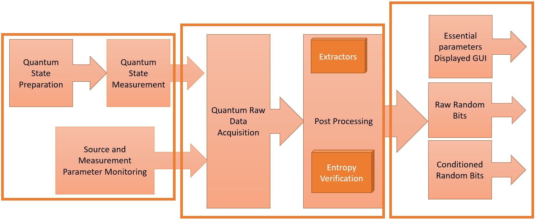
Figure 1: Quantum Noise Random Number Generator [15].

II Source of randomness

The quantum randomness in QRNG comes from the consumption of coherence. Since our QRNG method is based on the time of arrival principle hence, it is important to briefly discuss the coherent state and present a mathematical description of the photon. The coherent state $\alpha$ is the quantum mechanical counterpart of monochromatic light. It can be represented by amplitude and phase in a manner $\alpha=\left|\alpha\right|e^{i\theta}$. The complex number specifies the amplitude in photon number units.

II.1 Photon statistics within a time segment follows a Poisson distribution.

We know that a perfectly coherent light follows Poisson distribution [16]. Consider a beam segment corresponding to a predefined time segment with an average number of photon statistics as $\mu=\phi T$ where, $\phi$ is an average optical flux. We divide the time segment into small time bins and show that the probability of finding $n$ photons within a time segment $(T)$ containing $N$ time bins follow Poisson distribution. Let this probability be given by $P(n)$. Consider probability of finding $n$ time bins containing $1$ photon is $p_{1}=\mu/N$ and $N-n$ time bins containing no photons. This probability is given by a binomial distribution

$$\begin{array}[]{ccc}P(n)&=&\frac{N!}{n!(N-n)!}p_{1}^{n}(1-p_{1})^{N-n}\\ &=&\frac{N!}{n!(N-n)!N^{n}}\mu^{n}\left(1-\frac{\mu}{N}\right)^{N-n}\end{array}$$ (1)

We will take the limit as $N\rightarrow\infty$, the probability is $\underset{N\rightarrow\infty}{\textrm{lim}}[P(n)]=\frac{1}{n!}\mu^{n}e^{-\mu}$, thus, the probability of finding $n$ photons in $T$ time segment follows Poisson distribution $P(n)$. It is important to mention that we have considered ideal detectors with $100\,\%$ efficiency.

II.2 Quantum theory of photon detection

When conducting an experiment to leverage the Poisson nature of photon statistics of coherent light we have to consider the optical loss and imperfection in the devices. These are inefficient optics, absorption and imperfect detectors. These lead to a random sampling of photons which degrades the photon statistics. If we look at the quantum theory of photon detection [16], it aims to connect the photo count statistics of the detector within a time segment $T$ with photon statistics impinging at the detector. The variance in the photo count number is $\left(\triangle C\right)^{2}$ and the variance in the photon number is $\left(\triangle n\right)^{2}$. The relationship is established by

$$\left(\triangle C\right)^{2}=\eta^{2}\left(\triangle n\right)^{2}+\eta(1-\eta)\mu.$$ (2)

If the detector was perfect (i.e. $\eta=1)$ then the photon count statistics would have been equal to the photon statistics. Consider a coherent source (i.e. $\left(\triangle n\right)^{2}=\mu$) and an imperfect detector as in case of PMT or SPAD, the equation 2 will become $\left(\triangle C\right)^{2}=\mu\eta=C$ thus, the photo count statistics $(C)$ and photon statistics $(\mu)$ both follow Poisson distribution for all values of detection efficiencies.

III Time of arrival generators

The time of arrival based QRNG systems are based on encoding the arrival time of photons or pulses. During the short time periods, the arrival of a photon at the detector follows an exponentially distributed time $\lambda e^{-\mu T}$. The time between the two arrivals is the difference between two exponential random variables which is also exponential. The randomness in the exponential distribution is converted to a uniform bit sequence using post-processing algorithms. Another way to flatten the exponential distribution is by taking short time bins from an external reference and considering the time of arrivals within those bins. Nie et al. [13] has explained that when randomness is extracted from the mere arrival of time then the generated random numbers are biased. They have proposed a new method to generate uniform random numbers from the photon clicks at a fixed time duration $(t,t+T)$. The fixed time period is divided into small time bins with precision $t_{min}$. The time period is always less than the dead time allowing single detection. The advantage of this method is twofold, low-bias and large throughput compared to other methods of quantum random number generation.

III.1 Theoretical Analysis

The photon flux which is an average number of photons passing through a cross-section of a coherent beam follows a Poisson process. Precisely, a coherent beam with well-defined average photon number will follow a photon number fluctuation at a short time interval. The reason behind this fluctuation is due to the fact that we cannot predict the position of these photons. Consider a 1550 nm laser emitting 0 dBm of power, this will have an average flux of $7.78\times 10^{15}\textrm{ photons }s^{-1}$. If we apply $60$ dB attenuation the average flux will be $7.7\times 10^{9}\textrm{ photons }s^{-1}$. We can interpret this as an average of $7.7$ photons in the 1 ns time segment. Let us consider a time segment of 100 ps corresponding to an average flux of $0.77$. To summarize, if the coherent beam is attenuated to an extent that the beam segment contains few photons say on an average of $0.77$ photons and we make measurements of some $n$ samples, then, one can observe the random fluctuations in the photon number. This comes from the fact that the stimulated emission in the semiconductor laser is inherently random. Consider a time segment $T$, with mean photon number of $\mu T$, the probability distribution of $k$ photons arriving in time interval $T$ is given by $P(k)=\frac{e^{-\lambda\textrm{T}}(\mu T)^{k}}{k!}$. The photon number follows a Poisson distribution. Hence, the time interval between the arrival of consecutive photons also follows the Poisson process [3].

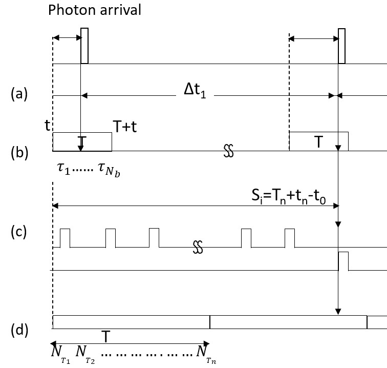
Figure 2: Timing diagram for arrival time of photon using different methods a) Wayne et al. [3], b) Nie et al. [13] , c) Yan et al. [14] and d) method proposed.

Consider $\lambda T=0.1$, there is $90.5\%$ probability of detecting no photons in $T$ time segment, $9\%$ of detecting single photons and finite probability of $0.5\%$ of multi photon in $T$ time segment. The time period is divided into $N_{b}$ time bins and each time bin is $\tau_{i}=(\frac{i-1}{N_{b}}T,\frac{i}{N_{b}}T)$. For an ideal detector $(\eta=1)$, there would have been multiple clicks in $T$, and first detection will be the minimum value of the random variable. However, the dead time is more than $T$ as a result there is a single detection in $T$. For a detection event the conditional probability of getting a detection at $i^{th}$ position given $k$ photons appear in that period is given by $P(\hat{n}=i\left|k\right)$. It is probability that detection happened at $\tau_{i}$ when $k$ photons are present in a period.

$$\begin{array}[]{ccc}P(\hat{n}=i\left|k\right)&=&\frac{P(i,k)P(T-\tau,k=0)}{P(k)}\\ &=&\frac{\frac{e^{-\lambda\tau_{i})}(\lambda(\frac{T-(i-1)T}{N_{b}}-\frac{T-iT}{N_{b}}))^{k}}{k!}}{\frac{e^{-\lambda T}(\lambda T)^{k}}{k!}}e^{-\lambda(T-\tau_{i})}\\ &=&\left(\frac{1-(i-1)}{N_{b}}-\frac{1-i}{N_{b}}\right)^{k}\\ &=&\left(\frac{1-(i-1)}{N_{b}}\right)^{k}-\left(\frac{1-i}{N_{b}}\right)^{k}\end{array}$$

The probability distribution function of the arrival of a photon conditioned on the fact that only $1$ photon is available in the time period $T$ is

$$\begin{array}[]{ccccccc}P(i,k=1)&=&\frac{1}{N_{b}}&=&\frac{1}{T/\tau}&=&\frac{\tau}{T}\end{array}.$$ (3)

Given a time period [13, 14], the probability of a photon to arrive at each time bin is $\frac{1}{N_{b}}$. In this expression, $\tau$ is the independent variable of the probability distribution function. The probability density is given by $\frac{1}{T}$. Thus, the arrival time is uniformly distributed in $[0,T].$ We have used binary code to encode the time bins. In Fig. 2, we have presented different methods for implementing time of arrival based QRNG. Wayne et al. [3] extracted random numbers by translating time intervals between detection into time bins. Nie et al. [13] generated raw quantum random numbers by considering time difference between photon click and an external time reference. The distribution of time difference between the external reference clock and photon click is approximately uniform. Yan et al. [14] have generated the highest reported raw data bits of $128$ Mbps by measuring the time of arrival from a common starting point. They convert each arrival time into sum of fixed period and phase time. Thereafter, they generate random numbers from phase time. In this work we address the arrival time of photon differently, we have considered an external reference as the basis of generation of raw bits. We have divided the external time reference $T$ into $N_{T}$ divisions. The arrival time is given by

$$A_{n}=\textrm{mod}[N_{b},N_{T_{i}}]$$ (4)

where, $N_{b}$ is the total number of random digits we want to generate. We do not restrict ourselves to modular arithmetic, the purpose is to segregate the time segment $T$ into $N_{T}$ fragments with each fragment equal to the precision of the measurement device. These fragments are distributed into $N_{b}$ divisions to generate $N_{b}$ random digits. The arrival of photon will be randomly falling in the range $1\leq N_{T_{i}}\leq N_{T}$, hence, applying the above equation [3, 13] we can prove that $N_{T_{i}}$ is uniformly distributed in $[0,T)$. In Table 1, we have compared the proposed work with existing works.

Table 1: Comparison of proposed QRNG with existing works on the basis of nature of source, detector, external reference clock, entropy per detection, precision of time measurement and throughput. CS stands for coherent source.

Ref.	Source	Detector	Ext ref	Entropy	Resolution	Rate
			(ns)	(ns)		(Mbps)
[3]	LED	SiAPD	-	5.5	5	40
[13]	CS	SiAPD	40.96	8	0.160	109
[14]	CS	SiAPD	20	8	20	128
AB	CS	InGaAs	500	16	0.005	2.4

III.2 Source of bias

To quantitatively evaluate the randomness of the raw data, we need to model the system carefully and figure out the facts that would introduce bias. There are a few major device imperfections to be examined.

1. The laser intensity needs to be constant. We have plotted the number of detections per $101\mu s$ to validate that the average photon count statistics is uniform. If the average photon number is 0.1 for 100 ns and $10\,\mu s$ dead time of detector. There should be one detection every 10100 ns or 10 clicks in 101 $\,\mu s$. We take 100 samples of 1010$\,\mu s$ intervals, and validate the mean photon number.

2. Detector dark counts are random clicks in absence of photons. It will be interesting to analyze the effect of random noise from dark counts getting mixed with random numbers generated from arrival times of photons. In the experiment, the dark count rate is roughly $350-400$ cps. Compared to the detection count rate, the proportion of dark count is much less therefore, it is not possible to conclusively state whether it introduces bias or not.

3. In one of our implementations, we have considered a dead time of $5\,\mu s$, in other, we have considered a dead time of $10\,\mu s$, which is far greater than the duration of external reference which is 100 ns (500 ns). The dead time can be considered as a drift [13] and it does not affect the quality of random numbers.

4. The probability for multi-photon emission from an attenuated CW laser is non-zero. If we consider detectors that can distinguish between multi-photon and single-photon then we can discard the multi-photon cases. This will reduce the bias in the output. However, we have considered the mean photon number much less than 1 and this would reduce the chances of multi-photon considerably.

IV Experimental analysis

The experimental setup is presented in Fig. 3, it comprises of Distributed Feedback (DFB) Laser operated in continuous mode. The laser diode has a wavelength of $1550$ nm and output power of $0.1$ mW. We have $2$ variable optical attenuators to tune the amplitude of weak coherent source to the desired value. One of them is kept fixed and the other is altered to achieve granularity. We have implemented SPD from CHAMPION Aurea detectors in free-running mode. It has the flexibility of adjusting at variable efficiencies, for example, $10\%$, $20\%$, and $30\%$ and the dead time can be configured to achieve the required count rate with respect to particular efficiency. We have considered different values of $N_{b}$ as 8, 100, 200, 256, 500 and 512 for external clock of 100 ns. When we implemented the scheme with 500 ns clock reference, we have considered 65536 divisions and generated 16 bits per detection. This implies that each division is 7.6 ps. The jitter in SPD is 180 ps and hence for better results, we should consider a division greater than this period. At $10\%$ efficiency and 10 $\mu s$ dead time the SPD has a 350-400 dark counts and counting rate of 90 Kcps, the photon flux at the input of SPD is $9\times 10^{6}$ cps corresponding to -89 dBm optical power with mean photo count of 0.09. When SPD has a counting rate of 96 Kcps, the photon flux at the input of SPD is $2.4\times 10^{7}$cps corresponding to -85 dBm optical power with a mean photo count of 0.24. However, at a continuous rate, we have considered the SPD count rate as $9\times 10^{4}$. We have presented the frequency distribution of the digits 1 to 256 generated randomly in Fig. 4. We find that the throughput is almost uniform. We have converted this to binary and tested it on the NIST test platform. We have performed Toeplitz hashing, however, the results were not improving the ENT or NIST tests. The raw numbers generated are unpredictable and uniform simultaneously, hence eliminating the need for applying any mathematical algorithm. At 5 $\mu s$ dead time we have considered a counting rate of 150 Kcps. We have used single time-to-digital converter (TDC), TDC_AS6501 in field-programmable gate array (FPGA) which is Zynq UltraScale+ MPSoC for post-processing the data. The TDC can respond to external clock reference from $2$ MHz to $12.5$ MHz. The TDC has an internal clock of 5 ps and it can count till 500 ns. An external reference with frequency 10 MHz in one implementation and 2 MHz in other implementation with a jitter of 3 ps is used as a reference clock which is edge synchronized with the TDC counter. The throughput at 150 Kcps count rate is 2.4 Mbps as raw QRNG data with $5\mu s$ dead time.

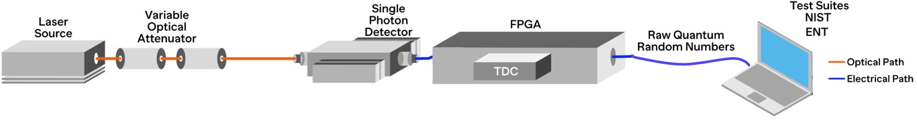
Figure 3: Experimental setup.

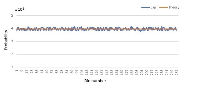
Figure 4: Probability distribution for theoretical vs experimental for 256 time bins with detection event of 90 Kb raw data.

Table 2: Results of ENT tests for a typical sequence of 1069712 bits.

ENT test item	QRNG	TRNG	Ideal value
Entropy (bits per bit)	1.000000	1.000000	1.000000
Chi-square distribution	45%	15.11%	10% $\sim$ 90%
Arithmetic mean value	0.4997	0.5001	0.5000
Monte Carlo value for Pi	3.1515369080	3.142180307	3.1415926536
Serial correlation coefficient	0.000590	0.000088	0.000000

V Entropy estimation

Entropy in the information-theoretic sense is a measure of randomness or unpredictability of the outputs of an entropy source. The larger the entropy, the greater the uncertainty in predicting the outcomes. Estimating the amount of entropy available from a source is necessary to see how many bits of randomness are available. If a discrete random variable $X$ has $n$ possible values where, the $i^{th}$ outcome has probability $p_{i}$ then, the Rényi entropy of order $\alpha$ is defined as

$$H_{\alpha}(X)=\frac{1}{1-\alpha}\log_{2}\left(\stackrel{{\scriptstyle[}}{{i}}=1]{n}{\sum}p_{i}^{\alpha}\right)$$ (5)

for $0\,\leq\,\alpha\,\leq\,\infty$. As $\alpha\rightarrow\infty$, the Rényi entropy of $X$ converges to the negative logarithm of the probability of the most likely outcome, called the min-entropy

$$H_{\infty}(X)=\underset{\alpha\rightarrow\infty}{\lim}H_{\alpha}(X)=-\log_{2}\max p_{i}.$$ (6)

The name min-entropy $(H_{\infty})$ stems from the fact that it is the smallest in the family of Rényi entropies. In this sense, it is the most conservative approach of measuring the unpredictability of a set of outcomes to measure the randomness content of a distribution. The standard Shannon entropy (which measures the average unpredictability of the outcomes) offers only a rough estimation of randomness. On the other hand, $H_{\infty}$ is used as a worst-case measure of the uncertainty associated with observations of $X$. This represents the best-case work for an adversary who is trying to guess an output from the noise source. For $H_{\infty}$, $p_{i}$ is the detection event probability at $i^{th}$ time bin and

$$H_{\infty}=-\frac{\log_{2}P_{max}}{\log_{2}N_{b}}=-\frac{\log_{2}P_{max}}{\textrm{bit}}=0.9971$$ (7)

from the maximum frequency of 0.00397 which is higher than [13]. In Fig. 4, the frequency distribution is almost uniform, the experimental value is close to theoretical value, in that case the entropy is approximately equal to 1 with high precision hence, in some works [14], entropy extraction is addressed by Shannon entropy.

$$H=-\stackrel{{\scriptstyle[}}{{i}}=1]{N_{b}}{\sum}p_{i}\textrm{log{\hbox{_{2}}}}p_{i},$$ (8)

The probability of detection event at each time bin is uniform thus, $p_{i}=\frac{1}{N_{b}}$. Hence, $H=\textrm{log${}_{2}$}N_{b}$, which means if we divide the time segment into $N_{b}=8,256$ or 1024 bins, we can generate 3, 8, or 10 random bits per photon arrival.

We have generated a 35 Gb random bitstream. Precisely, 63 files of 80 Mb data (total 5 Gb data) leading to raw QRNG data of 35-45 Gb. We performed 30 runs of 180 Mb random data files in the NIST STS test suite [17]. Raw QRNG data is of length 186504193 bits. We have tested 100 sequences of sample size $10^{6}$ bits. Some important statistical properties of generated random bitstreams are computed using the ENT program [18]. ENT is a series of basic statistical tests that evaluate the random sequence in some elementary features such as the equal probabilities of ones and zeros, the serial correlation, etc. The testing results with ENT are presented in Table 2. Each test in the NIST suite evaluates a p-value which should be larger than the significance level. The significance level in the tests is $\alpha=0.01$. The test is considered successful if all the p-values satisfy 0.01 $\leq$ p-value $\leq$ 0.99. Ten random data files with each file size of 100000 bits are tested. In the tests producing multiple outcomes of p-values, the worst outcomes are selected. The testing results with NIST are presented in Table 3. All the output p-values are larger than 0.01 and smaller than 0.99, which indicates that generated random bits well pass the NIST tests. We have compared the raw quantum random numbers with the NIST’s Blum-Blum-Shub algorithm and in-house TRNG built from FPGA from the asynchronous sampling of a ring oscillator.

Table 3: Results of NIST tests for a typical sequence of 100000 random bits.

NIST test item	BBS	QRNG	TRNG
	p value	p value	p-value
Frequency	0.816537	0.534146	0.213309
Block frequency	0.366918	0.122325	0.015598
Cumulative sums	0.955835	0.634146	0.851383
Runs	0.090936	0.739918	0.137282
Longest run	0.202268	0.534146	0.494392
Rank	0.202268	0.534146	0.383827
FFT	0.275709	0.350485	0.494392
Non overlapping template	0.764295	0.991468	0.883171
Overlapping template	0.455937	0.350485	0.779188
Universal	0.060806	0.213309	0.699313
Approximate entropy	0.971699	0.839918	0.739918
Random Excursions	0.534146	0.739918	0.186566
Random Excursions Variant	0.911413	0.457799	0.311542
Serial	0.739918	0.911413	0.779188
Linear complexity	0.145326	0.739918	0.289667

VI Conclusion

We have designed and tested a practical high-speed QRNG based on the time of arrival quantum entropy from a CW laser at telecommunication wavelength. This is the first work on time of arrival QRNG using InGaAs detectors. These detectors have a greater dead time than Silicon detectors enabling us to increase the external reference time to 500 ns compared to previous values of 40.6 ns [13] and 20 ns [14]. We have implemented precision time measurement of 5 ps which is reported for the first time. Hence, we could extract 16 bits of entropy from one photon arrival time. The photon arrival follows a Poisson distribution, an exponential waiting time introduces bias, this is overcome using external reference clock and we have generated uniform random numbers with high entropy particularly, min-entropy always greater than 0.99 value. The method of time measurement of photon is simpler in implementation and higher in precision time measurement than earlier works [13, 14, 3]. The proposed work can also be used to generate higher throughput by increasing the duration of the external reference clock however, the increase in throughput will be linear. We propose that implementing the time of arrival QRNG with InGaAs detectors and high precision time measurement will enable generating maximum entropy per detection event. The proposed work eliminates the use of any mathematical algorithm to generate uniform output hence, the random numbers produced from the system are derived from the quantum behavior of photons.

- [1] H. Schmidt, Quantum-mechanical random-number generator, J. Appl. Phys. 41, 462–468 (1970).
- [2] Y. Shen, L. Tian, and H. Zou, Practical quantum random number generator based on measuring the shot noise of vacuum states, Phys. Rev. A 81, 063814 (2010).
- [3] M. A. Wayne, E. R. Jeffrey, G. M. Akselrod and P. G. Kwiat, Photon arrival time quantum random number generation, J. Mod. Opt. 56:4, 516–522 (2009), DOI:10.1080/09500340802553244.
- [4] M. Stipcevic and B. M. Rogina, Quantum random number generator based on photonic emission in semiconductors, Rev. Sci. Instrum. 78, 045104 (2007).
- [5] C. Gabriel, C. Wittmann, D. Sych, R. Dong, W. Mauerer, U. L. Andersen, C. Marquardt and G. Leuchs, A generator for unique quantum random numbers based on vacuum states, Nat. Photonics 4, 711–715 (2010).
- [6] H. Guo, W. Tang, Y. Liu, and W. Wei, Truly random number generation based on measurement of phase noise of a laser, Phys. Rev. E 81, 051137 (2010).
- [7] A. Marandi, N. C. Leindecker, K. L. Vodopyanov and R. L. Byer, All-optical quantum random bit generation from intrinsically binary phase of parametric oscillators, Opt. Express 20, 19322–19330 (2012).
- [8] C. R. S. Williams, J. C. Salevan, X. Li, R. Roy and T. E. Murphy, Fast physical random number generator using amplified spontaneous emission, Opt. Express 18, 23584–23597 (2010).
- [9] M. Herrero-Collantes and J. C. Garcia-Escartin, Quantum random number generators, Rev. Mod. Phys. 89, 015004 (2017).
- [10] M. Wahl, M. Leifgen, M. Berlin, T. Röhlicke, H.-J. Rahn and O. Benson, An ultrafast quantum random number generator with provably bounded output bias based on photon arrival time measurements, Appl. Phys. Lett. 98, 171105 (2011).
- [11] S. Li, L. Wang, L.-An Wu, H.-Q. Ma, and G.-J. Zhai, True random number generator based on discretized encoding of the time interval between photons, J. Opt. Soc. Am. A 30, 124 (2013).
- [12] M. A. Wayne and P. G. Kwait, Low-bias high-speed quantum random number generator via shaped optical pulses, Opt. Express 18, 9351 (2010).
- [13] Y. Nie, H. Zhang, Z. Zhang, J. Wang, X. Ma, J. Zhang and J. Pan, Practical and fast quantum random number generation based on photon arrival time relative to external reference, Appl. Phys. Lett. 104, 051110 (2014).
- [14] Q. Yan, B. Zhao, Z. Hua, Q. Liao, and H. Yang, High-speed quantum-random number generation by continuous measurement of arrival time of photons, Rev. Sci. Instrum. 86, 073113 (2015), https://doi.org/10.1063/1.4927320.
- [15] Series X: Data Networks Open System Communications and security, Quantum communication Quantum noise random number generator architecture, Recommendation X.1702 (11/19).
- [16] Mark Fox, Quantum optics: an introduction, Oxford Univ. Press, Oxford, Oxford master series in atomic, optical, and laser physics (2006).
- [17] A. Rukhin, J. Soto, J. Nechvatal, M. Smid, E. Barker, S. Leigh, M. Levenson, M. Vangel, D. Banks, A. Heckert, J. Dray and S. Vo, NIST Special Publication 800-22 (NIST, 2008), http://csrc.nist.gov/rng/.
- [18] J. Walker, ENT: A Pseudorandom Number Sequence Test Program, http://www.fourmilab.ch/random.