Learning Contextualized Knowledge Structures
for Commonsense Reasoning

Abstract

Recently, knowledge graph (KG) augmented models have achieved noteworthy success on various commonsense reasoning tasks. However, KG edge (fact) sparsity and noisy edge extraction/generation often hinder models from obtaining useful knowledge to reason over. To address these issues, we propose a new KG-augmented model: Hybrid Graph Network (HGN). Unlike prior methods, HGN learns to jointly contextualize extracted and generated knowledge by reasoning over both within a unified graph structure. Given the task input context and an extracted KG subgraph, HGN is trained to generate embeddings for the subgraph’s missing edges to form a “hybrid” graph, then reason over the hybrid graph while filtering out context-irrelevant edges. We demonstrate HGN’s effectiveness through considerable performance gains across four commonsense reasoning benchmarks, plus a user study on edge validness and helpfulness.

1 Introduction

Commonsense reasoning (CSR) is essential for natural language understanding (NLU) systems to function effectively in the real world Apperly (2010). For example, to answer the question in Figure 1, one must already know that printing requires using paper. Yet, since commonsense knowledge is self-evident to humans, it is rarely stated in natural language Gunning (2018). This makes it hard for neural pre-trained language models (PLMs) (Devlin et al., 2019) to learn commonsense knowledge from corpora alone Marcus (2018).

Unlike raw text corpora, knowledge graphs (KGs) can provide structured commonsense facts (edges) of the form (concept1, relation, concept2) Speer et al. (2017). Hence, many recent CSR models augment the PLM with a KG, allowing such KG-augmented models to make predictions via multi-hop reasoning over the KG Lin et al. (2019); Bosselut and Choi (2019).

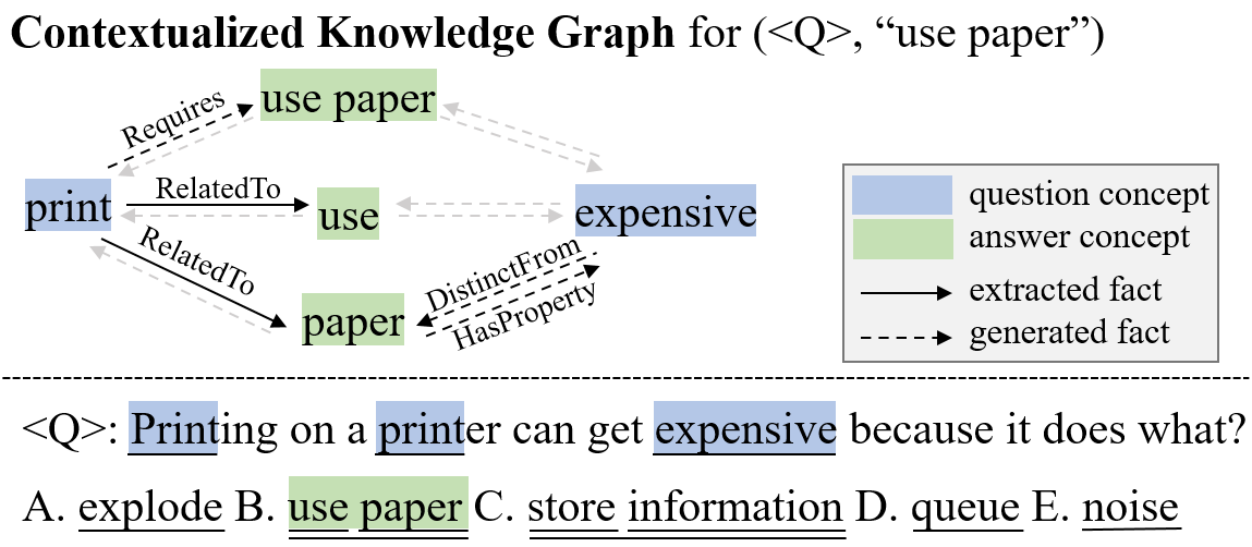
Figure 1: KG-Augmented Commonsense QA. Predicting the correct answer (“use paper”) requires commonsense facts like (print, Requires, paper) and (paper, HasProperty, expensive), which are not given in the question and candidate answers. HGN uses facts extracted from the KG, e.g., (print, RelatedTo, use), but also generates new facts, eventually upweighting relevant ones, e.g., (print, Requires, use paper) and (paper, HasProperty, expensive), while downweighting irrelevant ones, e.g., (use, ?, expensive).

Despite the growing success of KG-augmented models, obtaining helpful KG facts for a given task instance remains challenging. Existing models assume using either KG-extracted edges Lin et al. (2019); Ma et al. (2019); Feng et al. (2020); Yasunaga et al. (2021), PLM-generated edges (to address KG edge sparsity) Bosselut and Choi (2019), or a late fusion of both Wang et al. (2020) is sufficient. Both extraction and generation can produce unhelpful edges, so the model must decide which edges to focus on during reasoning. Since extracted and generated edges are derived from the same set of concepts (nodes), modeling the interactions between extracted and generated edges jointly within a shared KG structure could provide stronger signal for identifying contextually relevant edges. However, current models do not leverage this information.

In response, we propose a new KG-augmented model: Hybrid Graph Network (HGN). Unlike prior models, HGN learns to jointly contextualize extracted and generated knowledge by reasoning over both within a unified graph structure. Given the task input (i.e., context) and an extracted KG subgraph, HGN is trained to generate embeddings for the subgraph’s missing edges to form a “hybrid” graph, then reason over the graph (to update model parameters) while filtering out context-irrelevant edges. HGN achieves this primarily through edge reweighting, which downweights irrelevant edges, and edge-weighted message passing, which attenuates irrelevant edges’ impact on reasoning.

Our extensive experiments demonstrate that HGN improves performance over all baselines across four CSR benchmarks. In particular, among comparable methods, HGN ranks first on the CommonsenseQA (Talmor et al., 2019) and OpenbookQA (Mihaylov et al., 2018) leaderboards. Plus, our user studies show that humans find HGN-filtered edges to be more valid and helpful than the heuristically extracted edges used in prior work.

2 Problem Statement

We consider CSR tasks, like question answering (QA), which can benefit from commonsense KGs. To solve CSR tasks, we focus on KG-augmented models, where a PLM is augmented with a commonsense KG. Given a CSR task, let $x$ be the task’s text input, $f$ be the model, and $f(x)$ be the model output. We denote a KG as $\mathcal{G}=(\mathcal{V},\mathcal{R},\mathcal{E})$. $\mathcal{V}$, $\mathcal{R}$, and $\mathcal{E}$ are the sets of nodes (concepts), relations, and edges (facts), respectively, in the KG. An edge is a directed triple of the form $e=(h,r,t)\in\mathcal{E}$, where $h\in\mathcal{V}$ is the head node, $t\in\mathcal{V}$ is the tail node, and $r\in\mathcal{R}$ is the relation between $h$ and $t$. Let $[\cdot,\cdot]$ denote concatenation of text or vectors.

As illustrated in Figure 2, a KG-augmented model $f$ has three main components: text encoder $f_{\text{text}}$, graph encoder $f_{\text{graph}}$, and scoring function $f_{\text{score}}$. First, $\mathbf{s}=f_{\text{text}}(x;\bm{\uptheta}_{\text{text}})$ is the encoding of $x$, where $f_{\text{text}}$ is usually a Transformer PLM. Second, as supporting evidence, a $x$-specific graph $\mathcal{G}^{\prime}=(\mathcal{V}^{\prime},\mathcal{R}^{\prime},\mathcal{E}^{\prime})$ is constructed from $\mathcal{G}$ (Figure 1). Typically, this is done via heuristic extraction by selecting $\mathcal{V}^{\prime}\subseteq\mathcal{V}$ as the concepts mentioned in $x$, $\mathcal{R}^{\prime}\subseteq\mathcal{R}$ as the relations between concepts in $\mathcal{V}^{\prime}$, and $\mathcal{E}^{\prime}\subseteq\mathcal{E}$ as the edges involving $\mathcal{V}^{\prime}$ and $\mathcal{R}^{\prime}$. If $\mathcal{G}$ does not provide enough knowledge to build a good $\mathcal{G}^{\prime}$, then new edges are sometimes added to $\mathcal{G}^{\prime}$ using a PLM-based generator Wang et al. (2020). We call $\mathcal{G}^{\prime}$ the contextualized KG. $\mathbf{g}=f_{\text{graph}}(\mathcal{G}^{\prime},\mathbf{s};\bm{\uptheta}_{\text{graph}})$ is then the joint encoding of $\mathcal{G}^{\prime}$ and $\mathbf{s}$. Third, the model output is computed as $f(x)=f_{\text{score}}([\mathbf{s},\mathbf{g}];\bm{\uptheta}_{\text{score}})$, where $f_{\text{score}}$ is usually a multilayer perceptron (MLP). Existing KG-augmented models mainly differ in their design of $f_{\text{graph}}$, reasoning over the KG through message passing Schlichtkrull et al. (2018a); Feng et al. (2020); Yasunaga et al. (2021) or edge/path aggregation Lin et al. (2019); Bosselut and Choi (2019); Ma et al. (2019).

While KG-augmented models can be applied to any CSR task involving KGs (e.g., natural language inference), we consider multi-choice QA in this work. Given a question $q$ and set of candidate answers $\{a_{i}\}$, the QA model’s goal is to predict a plausibility score $\rho(q,a)$ for each $a\in\{a_{i}\}$, so that the highest score is predicted for the correct answer. To use KG-augmented models for commonsense QA, we set $x=[q,a]$ and $\rho(q,a)=f(x)$.

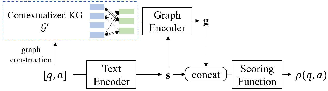
Figure 2: High-level schematic of a typical KG-augmented model for CSR. In KG-augmented models, text encoder $f_{\text{text}}$ tends to be a Transformer PLM, and scoring function $f_{\text{score}}$ is usually an MLP. Meanwhile, KG-augmented models generally vary more in their graph encoder $f_{\text{graph}}$ and graph construction.

3 Hybrid Graph Network (HGN)

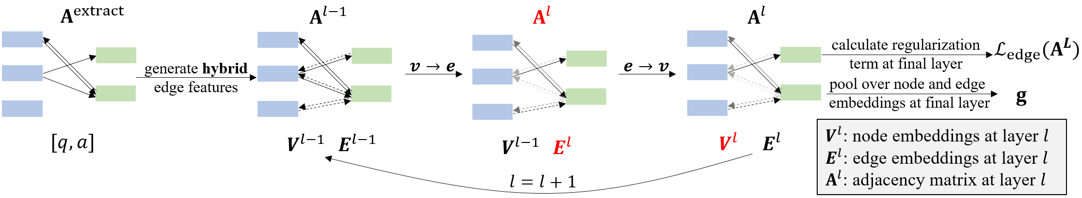
Figure 3: Overview of HGN. After building a hybrid graph of extracted and generated edges (§3.2), HGN reasons over the hybrid graph by updating the node embeddings $\mathbf{V}$, hybrid edge embeddings $\mathbf{E}$, and adjacency matrix $\mathbf{A}$ at each layer $\ell$ (§3.3). Darker edges indicate higher weights. Red variables are updated in the previous step.

3.1 Overview

As illustrated in §2 and Figure 2, given question-answer pair $(q,a)$ for an instance of the multi-choice QA task, the KG-augmented QA model first obtains a $(q,a)$-contextualized KG $\mathcal{G}^{\prime}$ via the full KG $\mathcal{G}$. Edges in $\mathcal{G}^{\prime}$ can be extracted directly from $\mathcal{G}$ or generated using a PLM-based generator Wang et al. (2020); Bosselut et al. (2019). Then, the model transforms $(q,a)$ and $\mathcal{G}^{\prime}$ into text encoding $\mathbf{s}$ and graph encoding $\mathbf{g}$, respectively. Finally, $\mathbf{s}$ and $\mathbf{g}$ are used to predict $(q,a)$’s plausibility.

However, a contextualized KG may have low knowledge recall or precision, hindering the QA model’s access to relevant knowledge. Low recall can stem from missing edges in $\mathcal{G}$, low precision can be the result of bad annotations in $\mathcal{G}$, and both can be caused by noisy edge extraction or generation when building $\mathcal{G}^{\prime}$. HGN addresses these issues by reasoning over both extracted and generated edges within a unified graph structure. To improve recall, HGN generates new edges via a PLM-based generator, then initializes a hybrid contextualized KG containing both extracted and generated edges. Note that edge generation is generally $(q,a)$-agnostic and may produce irrelevant edges that hurt knowledge precision. To improve precision, HGN learns to reweight edges in the hybrid graph and reason over the hybrid graph via edge-weighted message passing. This is akin to learning the hybrid graph’s structure and reduces the impact of irrelevant edges on reasoning. Additionally, to further encourage downweighting of noisy edges during reasoning, HGN is trained with entropy regularization on the learned edge weights.

The overall learning objective of HGN is defined as $\mathcal{L}=\mathcal{L}_{\text{task}}+\beta\mathcal{L}_{\text{edge}}$, where $\mathcal{L}_{\text{task}}$ is the loss for the downstream task (in our work, QA), $\mathcal{L}_{\text{edge}}$ is the entropy regularization term for edge weights, and $\beta\geq 0$ is a loss weight hyperparameter. In the following subsections, we first explain how the contextualized KG $\mathcal{G}^{\prime}$ is constructed as a hybrid graph, including its node embeddings $\mathbf{V}$, hybrid edge embeddings $\mathbf{E}$, and adjacency matrix $\mathbf{A}^{0}$ (§3.2). Next, we show how HGN uses edge-weighted message passing to update $\mathbf{V}$, $\mathbf{E}$, and $\mathbf{A}^{0}$ for $L$ layers (Figure 3), yielding a refined adjacency matrix $\mathbf{A}^{L}$ of learned edge weights (§3.3). Finally, we describe how $\mathcal{L}_{\text{task}}$ is computed using $\mathbf{s}$ and $\mathbf{g}$, while $\mathcal{L}_{\text{edge}}$ is calculated using $\mathbf{A}^{L}$ (§3.4).

3.2 Hybrid Graph Construction

Node Embeddings.

The first step of retrieving knowledge from $\mathcal{G}$ is concept grounding, which involves identifying text spans in $(q,a)$ that match nodes in $\mathcal{V}$. We define $\mathcal{V}^{\prime}$ as the set of all concepts mentioned in $(q,a)$, where $\mathcal{V}^{\prime}_{q}=\{v_{i}\}_{i=1}^{n_{q}}$ and $\mathcal{V}^{\prime}_{a}=\{v_{i}\}_{i=1}^{n_{a}}$ are the question and answer concepts, respectively. Each node $v_{i}\in\mathcal{V}^{\prime}$ is represented by an embedding $\mathbf{v}_{i}\in\mathbf{V}$, which can be initialized using BERT Devlin et al. (2019) or TransE Bordes et al. (2013).

Hybrid Edge Embeddings.

In $\mathcal{G}^{\prime}$, we loosen the definition of an edge to be $e_{(i,j)}=(v_{i},v_{j})\in\mathcal{E}^{\prime}$. We build fully-connected edges between question and answer nodes in $\mathcal{G}^{\prime}$. The set of edges in $\mathcal{G}^{\prime}$ is thus defined as $\mathcal{E}^{\prime}=(\mathcal{V}^{\prime}_{q}\times\mathcal{V}^{\prime}_{a})\cup(\mathcal{V}^{\prime}_{a}\times\mathcal{V}^{\prime}_{q})$. After concept grounding, we need an edge embedding $\mathbf{e}_{(i,j)}\in\mathbf{E}$ for each edge $e_{(i,j)}$. Let $\mathbf{R}$ be the relation embeddings for all relations in $\mathcal{R}$, obtained using TransE. Each extracted edge $(v_{i},r,v_{j})\in\mathcal{E}$ is thus initialized in $\mathcal{G}^{\prime}$ as $\mathbf{e}_{(i,j)}=\mathbf{r}\in\mathbf{R}$. However, due to edge sparsity, many edges do not have labeled relations and cannot be initialized this way.

Meanwhile, despite PLMs’ limitations in commonsense, they have shown some ability to encode commonsense knowledge (Davison et al., 2019; Petroni et al., 2019) and aid KG completion (Malaviya et al., 2019; Bosselut et al., 2019; Wang et al., 2020). Hence, we generate edge embeddings for all unlabeled edges by feeding each unlabeled edge into a GPT-2 Radford et al. (2019) based generator $f_{\text{gen}}(\cdot,\cdot)$. This is further explained in the “Edge Embedding Generation” paragraph.

In summary, edge embeddings are computed in a hybrid way: (1) If there exists $r\in\mathcal{R}$ such that $(v_{i},r,v_{j})\in\mathcal{E}$, then $\mathbf{e}_{(i,j)}=\mathbf{r}\in\mathbf{R}$. (2) Otherwise, $\mathbf{e}_{(i,j)}=f_{\text{adapt}}(f_{\text{gen}}(v_{i},v_{j}))$, where $f_{\text{adapt}}(\cdot)$ is an MLP used to transform $f_{\text{gen}}(v_{i},v_{j})$ into the same space as $\mathbf{r}$.

Edge Embedding Generation.

Inspired by recent work in PLM-based commonsense KG completion (Bosselut et al., 2019; Malaviya et al., 2019; Wang et al., 2020), we frame edge generation as text generation. First, for each extracted edge $(h,r,t)\in\mathcal{E}$, we first tokenize its node pair $(h,t)$ and relation label $r$. Let $\tilde{h}$, $\tilde{r}$, and $\tilde{t}$ be the respective token sequences of $h$, $r$, and $t$. Also, let $\$$ be the special separator token. Next, for each tokenized extracted edge, we train a GPT-2 model (Radford et al., 2019) to autoregressively generate the concatenated sequence $[\tilde{h},\$,\tilde{t},\$,\tilde{h},\tilde{r},\tilde{t}]$.

During inference, we only have unlabeled edges $(v_{i},v_{j})\in\mathcal{E}^{\prime}$, with no $r$. Thus, for each $(v_{i},v_{j})$, GPT-2 is given $s_{\text{input}}=[\tilde{v_{i}},\$,\tilde{v_{j}},\$]$ and asked to generate the missing tokens $s_{\text{pred}}=[\tilde{v_{i}},\tilde{r},\tilde{v_{j}}]$. Let $[x_{1},x_{2},...,x_{T}]=[s_{\text{input}},s_{\text{pred}}]$. The edge embedding for $(v_{i},v_{j})$ is then computed as $f_{\text{gen}}(v_{i},v_{j})=\frac{1}{T}\sum_{i=1}^{T}\mathbf{h}_{i}$, where $\mathbf{h}_{i}$ is the GPT-2 hidden state for $x_{i}$. See Appendix §A for more details.

Alternatively, we consider another edge generation approach proposed by Wang et al. (2020). Here, $f_{\text{gen}}(\cdot,\cdot)$ is trained to generate a relational path connecting $v_{i}$ to $v_{j}$, then pool the path into an edge embedding. The rationale for this approach is that such paths have been shown to contain useful semantic information about the relation between $v_{i}$ and $v_{j}$ (Neelakantan et al., 2015; Das et al., 2017; Wang et al., 2020).

Adjacency Matrix.

Before edge generation, $\mathcal{G}^{\prime}$ has binary adjacency matrix $\mathbf{A}^{\text{extract}}$, where $\mathbf{A}_{(i,j)}=1\Leftrightarrow\exists r,\text{s.t. }(v_{i},r,v_{j})\in\mathcal{E}$. After getting embeddings for all edges $(v_{i},v_{j})\in\mathcal{E}^{\prime}$, $\mathbf{A}^{\text{extract}}$ becomes $\mathbf{A}^{0}$, a denser binary adjacency matrix in which $\mathbf{A}^{0}_{(i,j)}=1\Leftrightarrow(v_{i},v_{j})\in\mathcal{E}^{\prime}$.

3.3 Hybrid Graph Reasoning

The procedure described in §3.2 yields a hybrid graph, containing unweighted edges between all question-answer node pairs. Constructing this hybrid graph may improve edge recall, but does not address precision. Some edges in the initial hybrid graph may be irrelevant to the question-answer pair, either due to noisy edge extraction or generation. HGN is thus designed to downweight irrelevant edges by converting the unweighted graph into a weighted one, then learning to reweight all hybrid edges during reasoning (Figure 3).

Learnable Adjacency Matrix.

Although $\mathbf{A}^{0}$ is a binary adjacency matrix, HGN populates it with learned edge attention weights and iteratively updates them over $L$ layers of reasoning. We denote the adjacency matrix at layer $\ell$ as $\mathbf{A}^{\ell}$, where $0\leq\mathbf{A}^{\ell}_{(i,j)}\leq 1$. Updating $\mathbf{A}^{\ell}$ can be viewed as softly contextualizing the hybrid graph’s structure with respect to $(q,a)$.

Edge-Weighted Message Passing.

Following the general Graph Network (GN) formulation proposed by Battaglia et al. (2018), HGN’s graph reasoning module consists of layer-wise node-to-edge ($v\rightarrow e$) and edge-to-node ($e\rightarrow v$) message passing functions. However, we equip HGN with a modified version of GN’s edge-to-node message passing function, in which each edge’s weight is used to rescale information flow on that edge. Intuitively, an edge’s weight signifies the edge’s relevance for reasoning about the given task instance. We also use text encoding $\mathbf{s}$ as global context throughout message passing.

Formally, HGN’s update rule at layer $\ell$ is:

$$\begin{split}v\rightarrow e:\mathbf{h}^{\ell}_{(i,j)}&=f^{\ell}_{v\rightarrow e}\left(\left[\mathbf{h}^{\ell-1}_{i},\mathbf{h}^{\ell-1}_{j},\mathbf{h}^{\ell-1}_{(i,j)},\mathbf{s}\right]\right);\\ w^{\ell}_{(i,j)}&=f^{\ell}_{w}\left(\left[\mathbf{h}^{\ell-1}_{(i,j)},\mathbf{s}\right]\right);\\ \mathbf{A}^{\ell}_{(i,j)}&=\frac{e^{w^{\ell}_{(i,j)}}}{\sum_{(s,t)\in\mathcal{E}^{\prime}}e^{w^{\ell}_{(s,t)}}},\\ e\rightarrow v:\mathbf{u}^{\ell}_{(i,j)}&=f^{\ell}_{u}\left(\left[\mathbf{h}^{\ell-1}_{i},\mathbf{h}^{\ell}_{(i,j)}\right]\right);\\ \mathbf{h}^{\ell}_{j}&=f^{\ell}_{e\rightarrow v}\left(\sum\nolimits_{i\in\mathcal{N}_{j}}\mathbf{A}^{\ell}_{(i,j)}\mathbf{u}^{\ell}_{(i,j)}\right).\end{split}$$ (1)

$N_{j}$ is the set of $v_{j}$’s incoming neighbors; $f^{\ell}_{v\rightarrow e}$, $f^{\ell}_{w}$, $f^{\ell}_{u}$ and $f^{\ell}_{e\rightarrow v}$ are MLPs; $\mathbf{h}_{(i,j)}^{0}=\mathbf{e}_{(i,j)}$ is the initial embedding for edge $(v_{i},v_{j})$; and $\mathbf{h}_{i}^{0}=\mathbf{v}_{i}$ is the initial embedding for node $v_{i}$.

In node-to-edge message passing, the embedding of each edge $(v_{i},v_{j})\in\mathcal{E}^{\prime}$ is updated as $\mathbf{h}^{\ell}_{(i,j)}$, a function of $(v_{i},v_{j})$’s constituent nodes and the given context $\mathbf{s}$. Through $\mathbf{s}$, the hybrid graph is strongly contextualized with respect to $(q,a)$. Then, $\mathbf{h}^{\ell}_{(i,j)}$ is used to compute edge score $w^{\ell}_{(i,j)}$, which measures the edge’s relevance to $\mathbf{s}$. Each edge score is globally normalized across all edges in the graph to produce edge attention weight $\mathbf{A}^{\ell}_{(i,j)}$, so that low-scoring edges are softly pruned by receiving close-to-zero weight.

We use global edge attention (i.e., normalizing across $\mathcal{E}^{\prime}$) instead of local edge attention (i.e., normalizing across $N_{j}$) because local edge attention assumes at least one edge in $N_{j}$ is relevant, which may not be true. For example, given an irrelevant or incorrectly grounded concept, none of its edges will be helpful, and so all nodes in its neighborhood should be excluded from influencing the reasoning process. To demonstrate the advantage of global edge attention, we empirically compare our default HGN architecture to an HGN variant based on Graph Attention Network (GAT) (Velickovic et al., 2018), which uses local edge attention, in our experiments.

In edge-to-node message passing, the embedding of each node $v_{j}\in\mathcal{V}^{\prime}$ is updated as $\mathbf{h}^{\ell}_{j}$, a function of $v_{j}$’s neighboring edges. For each edge neighbor, edge weight $\mathbf{A}_{(i,j)}^{\ell}$ is used to rescale the edge’s influence on $v_{j}$’s embedding update.

3.4 Learning Objective

Task Loss.

After $L$ layers of message passing, we obtain node embeddings $\{\mathbf{h}^{L}_{i}\mid i:v_{i}\in\mathcal{V}^{\prime}\}$ and edge embeddings $\{\mathbf{h}^{L}_{(i,j)}\mid(i,j):(v_{i},v_{j})\in\mathcal{E}^{\prime}\}$. Node embeddings are aggregated into $\mathbf{v}_{\text{agg}}$ via attentive pooling with $\mathbf{s}$ as the query vector. Edge embeddings are aggregated into $\mathbf{e}_{\text{agg}}$ via edge-weighted sum pooling. The final graph encoding is then given as $\mathbf{g}=[\mathbf{v}_{\text{agg}},\mathbf{e}_{\text{agg}}]$. The probability of $a$ being the answer to $q$ is calculated as $\hat{\rho}(q,a)\propto\exp(\rho(q,a))$, where $\rho(q,a)=f_{\text{score}}([\mathbf{s},\mathbf{g}];\bm{\uptheta}_{\text{score}})$. We use cross-entropy loss for the QA classification task, so the loss for each $(q,a)$ with label $y$ is:

$$\mathcal{L}_{\text{task}}\left(\hat{\rho}(q,a;\bm{\uptheta})),y\right)=-y\log\hat{\rho}(q,a;\bm{\uptheta}).$$ (2)

Entropy Regularization.

To encourage the model to be decisive during edge reweighting, we use a regularization term to penalize non-discriminative edge weights. In an extreme case, a blind model will assign the same weight to all edges, degenerating $\mathcal{G}^{\prime}$ into an unweighted graph. This is a failure mode, since $\mathcal{G}^{\prime}$ is likely to contain mostly irrelevant edges, and we want the model to focus on the helpful edges. Therefore, via $\mathcal{L}_{\text{edge}}$, we train the model to minimize the entropy of the edge weight distribution (i.e., make the distribution more skewed), in order to maximize the informativeness of the predicted edge weights. Lower entropy means the model has higher certainty about edges’ relevance to the given task instance, such that the model will discriminatively judge some edges as being much more relevant than others. $\mathcal{L}_{\text{edge}}$ is computed as:

$$\begin{split}\mathcal{L}_{\text{edge}}(\mathbf{A}^{L}(q,a))=-\sum_{(i,j):(v_{i},v_{j})\in\mathcal{E}^{\prime}}\mathbf{A}^{L}_{(i,j)}\log\mathbf{A}^{L}_{(i,j)}.\end{split}$$ (3)

Joint Learning.

We jointly optimize $\mathcal{L}_{\text{task}}$ and $\mathcal{L}_{\text{edge}}$, so graph reasoning and structure can be jointly learned. The full learning objective is:

$$\begin{split}\begin{aligned} \mathcal{L}(\bm{\uptheta})=\sum_{(q,a,y)\sim X_{\text{train}}}&\Big{[}\mathcal{L}_{\text{task}}\left(\hat{\rho}(q,a)),y\right)+\beta\cdot\mathcal{L}_{\text{edge}}(\mathbf{A}^{L}(q,a))\Big{]},\end{aligned}\end{split}$$ (4)

where $\bm{\uptheta}=\{\bm{\uptheta}_{\text{text}},\bm{\uptheta}_{\text{graph}},\bm{\uptheta}_{\text{score}}\}$ is the set of all learnable parameters, and $X_{\text{train}}$ is the training set. We train our model end-to-end by minimizing $\mathcal{L}(\bm{\uptheta})$ with the RAdam (Liu et al., 2020) optimizer.

4 Experiments

Methods	BERT-Base		BERT-Large		RoBERTa
	60% Train	100% Train	60% Train	100% Train	60% Train	100% Train
LM Finetuning∗	52.06 ($\pm$0.72)	53.47 ($\pm$0.87)	52.30 ($\pm$0.16)	55.39 ($\pm$0.40)	65.56 ($\pm$0.76)	68.69 ($\pm$0.56)
RN∗ (Santoro et al., 2017)	54.43 ($\pm$0.10)	56.20 ($\pm$0.45)	54.23 ($\pm$0.28)	58.46 ($\pm$0.71)	66.16 ($\pm$0.28)	70.08 ($\pm$0.21)
RN + Link Prediction∗	-	-	53.96 ($\pm$0.56)	56.02 ($\pm$0.55)	66.29($\leavevmode\nobreak\ \pm$0.29)	69.33 ($\pm$0.98)
RGCN∗ (Schlichtkrull et al., 2018b)	52.20 ($\pm$0.31)	54.50 ($\pm$0.56)	54.71 ($\pm$0.37)	57.13 ($\pm$0.36)	68.33 ($\pm$0.85)	68.41 ($\pm$0.66)
GAT (Velickovic et al., 2018)	53.05 ($\pm$0.37)	56.51 ($\pm$0.74)	55.80 ($\pm$0.53)	58.18 ($\pm$1.07)	69.63 ($\pm$0.42)	71.20 ($\pm$0.72)
GN (Battaglia et al., 2018)	53.67 ($\pm$0.45)	55.65 ($\pm$0.51)	54.78 ($\pm$0.61)	57.81 ($\pm$0.67)	68.78 ($\pm$0.67)	71.12 ($\pm$0.45)
GconAttn∗ (Wang et al., 2019a)	51.36 ($\pm$0.98)	54.41 ($\pm$0.50)	54.96 ($\pm$0.69)	56.94 ($\pm$0.77)	68.09 ($\pm$0.63)	69.88 ($\pm$0.47)
KagNet∗ (Lin et al., 2019)	-	56.19	-	57.16	-	-
MHGRN∗ (Feng et al., 2020)	54.12 ($\pm$0.49)	56.23 ($\pm$0.82)	56.76 ($\pm$0.21)	59.85 ($\pm$0.56)	68.84 ($\pm$1.06)	71.11 ($\pm$0.81)
PathGenerator∗ (Wang et al., 2020)	54.44 ($\pm$0.42)	56.99 ($\pm$0.41)	57.53 ($\pm$0.19)	59.07 ($\pm$0.30)	69.46 ($\pm$0.23)	72.68 ($\pm$0.42)
HGN (w/ PathGen edges)	55.68 ($\pm$0.29)	57.77 ($\pm$0.39)	58.19 ($\pm$0.27)	60.89 ($\pm$0.19)	70.95 ($\pm$0.21)	73.41 ($\pm$0.31)
HGN (w/ RelGen edges)	55.72 ($\pm$0.32)	58.01 ($\pm$0.29)	58.19 ($\pm$0.11)	61.11 ($\pm$0.21)	71.10 ($\pm$0.11)	73.64 ($\pm$0.30)

Table 1: Accuracy on CommonsenseQA inhouse test set. Both our model variants significantly improve over all baselines. We use the same inhouse split as Lin et al. (2019). For baselines with ^∗, we use the reported numbers from Feng et al. (2020) and Wang et al. (2020) if available. Mean and standard deviation of four seeds are presented for all models except KagNet.

4.1 Experimental Setup

We evaluate our proposed model on four multiple-choice commonsense QA datasets: CommonsenseQA (Talmor et al., 2019), CODAH  (Chen et al., 2019), OpenBookQA (Mihaylov et al., 2018) and QASC (Khot et al., 2020) (details in Appendix §B). We use ConceptNet (Speer et al., 2017), a commonsensense knowledge graph, as $\mathcal{G}$. For text encoder $f_{\text{text}}$, we experiment with BERT-Base, BERT-Large (Devlin et al., 2019) and RoBERTa(-Large) (Liu et al., 2019) to validate our model’s effectiveness over different text encoders. For OpenbookQA and QASC, retrieving related facts from the provided corpus plays an important role in boosting the model’s performance. Therefore, we build our graph reasoning model on top of retrieval-augmented methods on the leaderboard: “AristoRoBERTa” for OpenBookQA and “RoBERTa (2-step IR)” for QASC. In this way, we can study if strong retrieval-augmented methods can still benefit from KG knowledge and our HGN framework.

4.2 Compared Methods

We compare our model with a series of KG-augmented methods and different graph encoders:

Models Using Extracted Facts.

We consider seven models that only use extracted facts. RN (Santoro et al., 2017) builds the graph with the same node set as our method but extracted edges only. The graph vector is calculated as $\mathbf{g}=\text{Pool}(\{\text{MLP}([\mathbf{v}_{i},\mathbf{e}_{(i,j)},\mathbf{v}_{j}])\mid(v_{i},v_{j})\in\mathcal{E}^{\prime}\})$. GN (Battaglia et al., 2018) presents a general formulation of GNNs. We instantiate it with the layerwise propagation rule defined in Equation 1. It differs from our HGN in that: (1) it only considers extracted edges; (2) all edge weights are fixed to 1. MHGRN (Feng et al., 2020) generalizes GNNs with multi-hop message passing. GAT (Velickovic et al., 2018) adopts attention mechanism to reweight edges locally in each node’s neighborhood. We implement it by replacing the graph edge attention with local edge attention and only considering $\mathcal{L}_{\text{task}}$ during training. RGCN (Schlichtkrull et al., 2018a) extends Graph Convolutional Networks (GCNs) (Kipf and Welling, 2017) with relation-specific transition matrices during message passing. It operates on the same graph as RN. The graph vector is calculated as $\mathbf{g}=\text{Pool}(\{\mathbf{h}^{L}_{i}\mid v_{i}\in V\})$. GconAttn (Wang et al., 2019b) softly aligns the nodes in question and answer and do pooling over all matching nodes to get $\mathbf{g}$. KagNet (Lin et al., 2019) uses an LSTM to encode relational paths between question and answer concepts and pool over the path embeddings for graph encoding.

Models Using Extracted and Generated Facts.

We consider two models that use both extracted facts and generated facts. RN + Link Prediction differs from RN by only considering the generated relation (predicted using TransE (Bordes et al., 2013)) between question and answer concepts. PathGenerator (Wang et al., 2020) learns a path generator from paths collected through random walks on the KG. The learned generator is used to generate paths connecting question and answer concepts. $\mathbf{g}$ is calculated as the concatenation of the pooled vector over the generated paths and the pooled vector over the extracted paths.

Our Model’s Variants.

As described in §3.2, the edge embedding can be computed either as a relation embedding or a path embedding. We name these two variants as HGN (w/ RelGen edges) and HGN (w/ PathGen edges) respectively.

Methods	Single	Ensemble
ALBERT+DESC-KCR (Xu et al., 2020)	80.7	83.3
ALBERT+KD	80.3	80.9
ALBERT+KCR	79.5	-
Unified QA (Khashabi et al., 2020)	79.1	-
ALBERT+KRD	78.4	-
T5-3B (Raffel et al., 2020)	78.1	-
ALBERT+HGN (w/ RelGen edges)	77.3	80.0
TeGBERT	76.8	-
ALBERT+PathGenerator (Wang et al., 2020)	75.6	78.2
ALBERT (Lan et al., 2020)	-	76.5

Table 2: Leaderboard of CommonsenseQA. HGN ranks first among comparable systems, especially achieving remarkable improvement over PathGenerator (Wang et al., 2020).

Methods	BERT-Large	RoBERTa
LM Finetuning	65.74	83.14
RN (Santoro et al., 2017)	64.59	82.45
RGCN (Schlichtkrull et al., 2018b)	65.56	82.42
GAT (Velickovic et al., 2018)	65.88	82.78
GN (Battaglia et al., 2018)	65.52	82.06
GconAttn (Wang et al., 2019a)	65.17	82.35
MHGRN (Feng et al., 2020)	65.92	83.07
PathGenerator (Wang et al., 2020)	64.67	82.27
HGN (w/ PathGen edges)	66.21	84.32
HGN (w/ RelGen edges)	66.75	84.08

Table 3: Test accuracy on CODAH. Both our model variants consistently improve over all baselines. We use the official split for 5-fold cross validation. Mean accuracy on 5 folds are presented.

Datasets	OpenBookQA	QASC
Base Models	AristoRoBERTa	RoBERTa (2-step IR)
LM Finetuning∗	77.40 ($\pm$1.64)	73.34 ($\pm$0.71)
RN∗ (Santoro et al., 2017)	78.05 ($\pm$0.77)	72.77 ($\pm$1.50)
RN + Link Prediction∗	77.25 ($\pm$1.11)	-
RGCN∗ (Schlichtkrull et al., 2018b)	74.60 ($\pm$2.53)	72.23 ($\pm$1.36)
GAT (Velickovic et al., 2018)	78.20 ($\pm$1.22)	72.61 ($\pm$0.93)
GN (Battaglia et al., 2018)	77.25 ($\pm$0.91)	72.53 ($\pm$0.70)
GconAttn∗ (Wang et al., 2019a)	71.80 ($\pm$1.21)	72.72 ($\pm$1.66)
MHGRN (Feng et al., 2020)	77.75 ($\pm$0.38)	73.24 ($\pm$0.45)
PathGenerator∗ (Wang et al., 2020)	79.15 ($\pm$0.78)	72.96 ($\pm$0.68)
HGN (w/ PathGen edges)	80.05 ($\pm$0.54)	74.10 ($\pm$0.42)
HGN (w/ RelGen edges)	80.15 ($\pm$0.38)	74.27 ($\pm$0.31)

Table 4: Test accuracy on OpenBookQA and QASC with retrieval-augmented methods as base models. Both our model variants greatly improve over all baselines except HGN (w/ PathGen edges) over MHGRN. For OpenbookQA baselines with ^∗, we use reported numbers from Wang et al. (2020). Mean and standard deviation of four seeds are presented.

Methods	Text Encoder	Test Acc
UnifiedQA (Khashabi et al., 2020)	T5-11B	87.2
T5-11B + KB	T5-11B	85.4
T5-3B (Raffel et al., 2020)	T5-3B	83.2
PathGenerator (Wang et al., 2020)	ALBERT	81.8
HGN (w/ RelGen edges)	AristoRoBERTa	81.4
AristoRoBERTa + KB	AristoRoBERTa	81.0
MHGRN (Feng et al., 2020)	AristoRoBERTa	80.6
PathGenerator (Wang et al., 2020)	AristoRoBERTa	80.2
KF + SIR (Banerjee and Baral, 2020)	RoBERTa	80.2
AristoRoBERTa	AristoRoBERTa	80.2

Table 5: Leaderboard of OpenBookQA. Our HGN ranks first among all submissions using AristoRoBERTa as the text encoder.

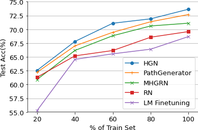
(a)

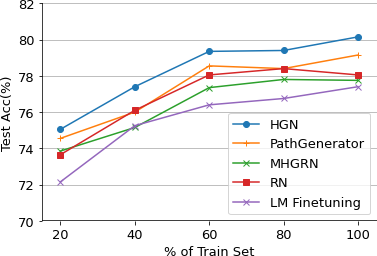
(b)

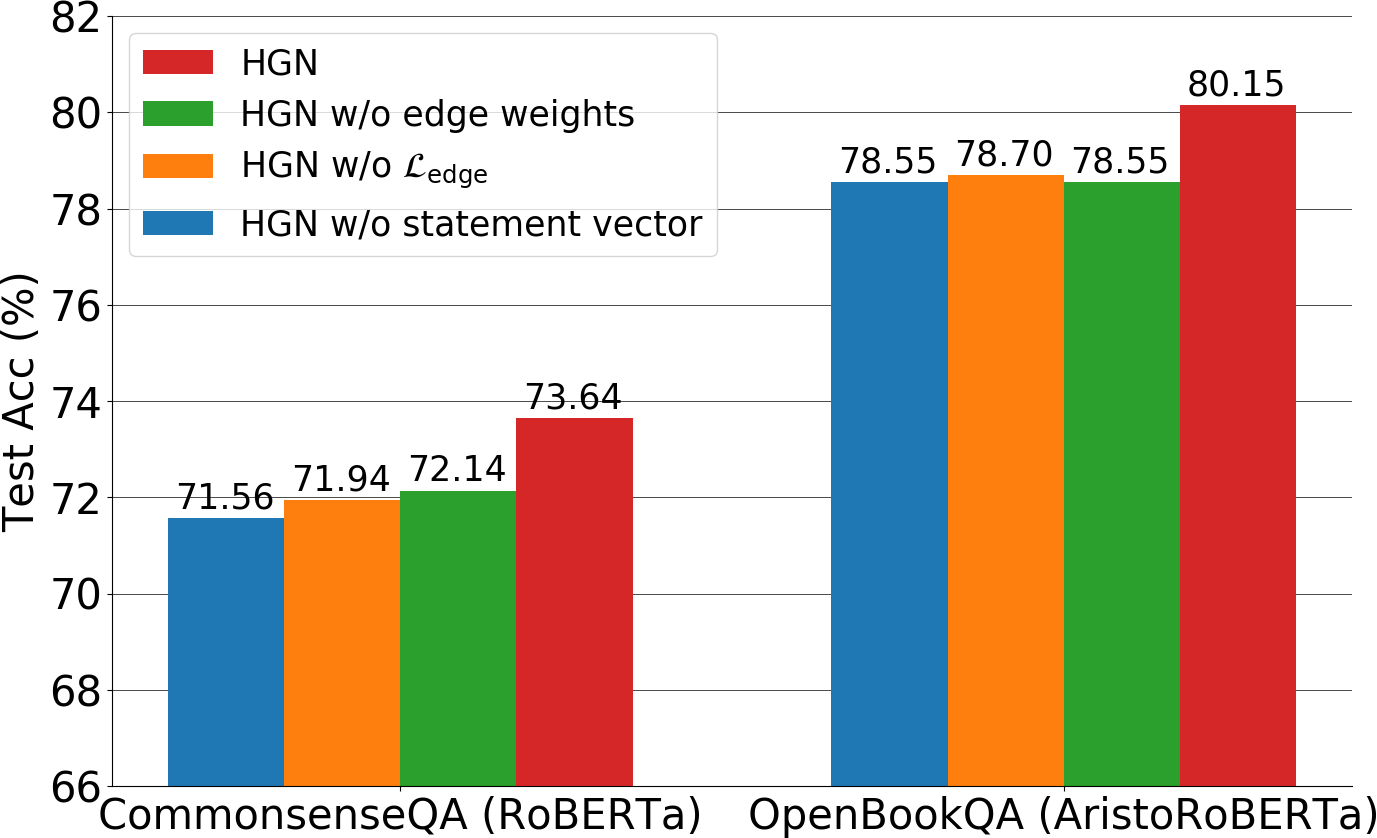
(c)

Figure 4: Low-resource and ablation studies. (a)(b) Performance of HGN and baseline models with different amounts of training data; (c) Performance of different model variants.

4.3 Results

Performance Comparisons.

Tables 1,  3,  4 show performance comparisons between our models and baseline models on CommonsenseQA, CODAH, OpenBookQA and QASC. We clearly find that models with stronger text encoders perform better (i.e. RoBERTa $>$ BERT-Large $>$ BERT-Base). For all text encoders, our HGN shows consistent improvement over baseline models on all datasets. The improvement over all baselines are tested to be statistically significant under most settings, demonstrating the effectiveness of HGN both with and without retrieved evidence.

We also submit our best model to leaderboards for CommonsenseQA and OpenBookQA. For CommonsenseQA (Table 2), our HGN ranks first among comparable approaches and shows remarkable improvement over PathGenerator (Wang et al., 2020) and the LM Finetuning approach (ALBERT (Lan et al., 2020)). Higher-ranking models either use stronger text encoders or leverage additional data resources. Specifically, UnifiedQA (Khashabi et al., 2020) and T5-3B (Raffel et al., 2020) are based on T5. They have 11B and 3B parameters respectively, making them impractical to be finetuned in an academic setting. ALBERT+DESC-KCR (Xu et al., 2020) and ALBERT+KD additionally use concept definitions from dictionaries. ALBERT+DESC-KCR and ALBERT+KCR leverage “question_concept” annotations, which are used during the construction of the CommmonsenseQA dataset and allow the model to learn shortcuts that don’t generalize to other datasets. ALBERT+KRD retrieve sentences from OMCS corpus (Liu and Singh, 2004) as input. These methods are therefore not comparable with our model. For OpenBookQA (Table 5), our model ranks first among all models using AristoRoBERTa as the text encoder.

Training with Less Labeled Data.

Figure 4 (a)(b) show the results of our model and baselines when trained with different portions of the training data on CommonsenseQA and OpenBookQA. Our model gets better test accuracy under all settings. On CommonsenseQA without retrieved evidence, the improvement over the knowledge-agnostic baseline (LM Finetuning) is generally more significant with less training data, which suggests that incorporating external knowledge is helpful in the low-resource setting.

Study on More Model Variants.

To better understand the model design, we experiment with three variants of HGN (w/ RelGen edges) on CommonsenseQA and OpenBookQA. HGN w/o statement vector doesn’t consider $\mathbf{s}$ in Equation 1, which isolates the graph encoder from the text encoder. HGN w/o $\mathcal{L}_{\text{edge}}$ does not consider the entropy regularization term and thus does not penalize non-discriminative edge weights. HGN w/o edge weights reasons over an unweighted graph with hybrid features, which means edge weights are all fixed to 1 during training. Figure 4 (c) shows the results of the ablation study. “HGN” outperforms “HGN w/o $\mathcal{L}_{\text{edge}}$”, suggesting the usefulness of our proposed entropy regularization. Comparing “HGN w/o statement vector” with “HGN”, we find that accessing context information is also important for graph reasoning, which means information propagation and edge weight prediction should be conducted in a context-aware manner. HGN also improves over “HGN (w/o edge weights)”, indicating the effectiveness of conducting context-dependent pruning.

Contextualized Graph	GN ($\mathbf{A}^{\text{extract}}$)	HGN ($\mathbf{A}^{L}$)
Number of Edges	3.65 ($\pm$2.73)	4.38 ($\pm$3.24)
Number of Valid Edges	2.67 ($\pm$1.95)	3.15 ($\pm$1.98)
Percentage of Valid Edges	71.64%	78.51%
Average Helpfulness Score of Edges	0.90 ($\pm$0.50)	1.16 ($\pm$0.51)
Prune Rate	-	22.84%

Table 6: User studies on learned graph structures. 30 pairs of contextualized graphs output by GN and HGN are evaluated by 5 annotators.

4.4 User Study on Learned Structures

To assess HGN’s ability to refine graph structure, we compare the graph structure before and after being processed by HGN. Specifically, we sample 30 questions with its answer from CommonsenseQA’s development set and ask 5 human annotators to evaluate the graph output by GN (with adjacency matrix $\mathbf{A}^{\text{extract}}$ and extracted facts only) and by HGN (with adjacency matrix $\mathbf{A}^{L}$). We manually binarize $\mathbf{A}^{L}$ by removing edges with weight lower than $0.01$.

Given a graph, for each edge (fact), annotators are asked to rate its validness and helpfulness. The validness score is rated as a binary value in a context-agnostic way: 0 (the fact does not make sense), 1 (the fact is generally true). The helpfulness score measures if the fact is helpful for solving the question and is rated on a 0 to 2 scale: 0 (the fact is unrelated to the question and answer), 1 (the fact is related but doesn’t directly lead to the answer), 2 (the fact directly leads to the answer). Note that the percentage of valid edges can be understood as the precision of graph edges. For a given instance, the number of valid edges is proportional to the recall of the edges. We also include another metric named “prune rate” calculated as: $1-\frac{\text{\# edges in binarized }\mathbf{A}^{L}}{\text{\# edges in }\mathbf{A}^{0}}$, which measures the portion of edges assigned very low weights (softly pruned) during training and is only applicable to HGN.

The mean ratings for 30 pairs of (GN, HGN) graphs by 5 annotators are reported in Table 6. The Fleiss’ Kappa (Fleiss, 1971) is 0.51 (moderate agreement) for validness and 0.36 (fair agreement) for helpfulness. The graph refined by HGN has both more edges and denser valid edges compared to the extracted one. The refined graph also achieves a higher average helpfulness score. These all indicate that our HGN learns a superior graph structure with more helpful edges and fewer noisy edges, which improves over previous works that rely on extracted and static graphs. Detailed cases can be found in Appendix §C.

5 Related Work

Commonsense QA.

Commonsense QA is challenging because the required commonsense knowledge is seldom given in the question-answer context or encoded in the PLM’s parameters. Thus, many works obtain this knowledge from external sources (e.g., KGs, corpora). While Lv et al. (2020) show that KGs and corpora can provide complementary knowledge, our paper focuses on improving the use of KG knowledge. KG knowledge can be acquired in different ways, either from KG-extracted edges Lin et al. (2019); Ma et al. (2019); Feng et al. (2020); Yasunaga et al. (2021), PLM-generated edges Bosselut and Choi (2019), or both Wang et al. (2020). KG-augmented models mainly differ in how they encode KG knowledge, using message passing Schlichtkrull et al. (2018a); Feng et al. (2020) or edge/path aggregation Lin et al. (2019); Bosselut and Choi (2019); Ma et al. (2019); Wang et al. (2020). The most relevant work to ours is Wang et al. (2020). The main difference is that they coarsely combine extracted and generated knowledge via late fusion, while HGN encodes both types of knowledge within a unified graph. Besides, they use RN to pool over a set of paths for graph encoding, while HGN reasons over the graph via message passing and edge reweighting.

Graph Structure Learning.

Instead of assuming a fixed graph structure, a number of graph models learn the graph structure with respect to the downstream task. Some models learn to discretely select edges for the graph (i.e., hard pruning). Kipf et al. (2018) and Franceschi et al. (2019) sample the graph structure from a predicted probabilistic distribution with differentiable approximations. Norcliffe-Brown et al. (2018) calculate the relatedness between any pair of nodes and only keep the top-$k$ strongest connections for each node to construct the edge set. Sun et al. (2019) start with a small graph and iteratively expand it with retrieving operations. Others learn to reweight edges in a fully connected graph (i.e., soft pruning). Jiang et al. (2019) and Yu et al. (2019) propose heuristics for regularizing edge weights. Hu et al. (2019) use the question embedding to help predict edge weights. Unlike other edge reweighting models, HGN operates over a hybrid graph of both extracted and generated edges, while updating edge weights with respect to node, edge, and text features.

6 Conclusion

In this paper, we propose HGN, a KG-augmented model for CSR. To address KG edge sparsity and noisy edge extraction/generation, HGN learns to jointly contextualize extracted and generated knowledge by reasoning over both within a unified graph structure. We justify HGN’s design by showing that HGN improves performance on various CSR benchmarks and user studies. In future work, we plan to increase the graph’s relation expressiveness by incorporating open relations, plus make the edge extraction/generation process more dependent on the reasoning context.

Appendix A Implementation Details of Edge Embedding Generator (RelGen)

Here, we give a more detailed explanation of the PLM-based edge embedding generator $f_{\text{gen}}$, introduced in the “Edge Embedding Generation” paragraph of §3.2.

To implement $f_{\text{gen}}$, we adopt GPT-2 (Radford et al., 2019), which is pretrained on large corpora and achieves great success on a wide range of tasks involving sentence generation, as a generator to generalize the facts from the knowledge graph. We first convert each fact $(h,r,t)\in\mathcal{E}$ into a word sequence with a “prompt-generation” format: $\left[\tilde{h},\$,\tilde{t},\$,\tilde{h},\tilde{r},\tilde{t}\right]$, where $\tilde{h},\tilde{r},\tilde{t}$ are the word sequence of $h,r,t$ respectively, $\$$ denotes the delimiter token used by GPT-2, and $[\cdot,\cdot]$ denotes word sequence concatenation. We adopt this format because $\left[\tilde{h},\tilde{r},\tilde{t}\right]$ is similar to a natural language fact. Generating facts in a natural format helps induce commonsense knowledge stored in GPT-2 (Bosselut et al., 2019). We denote the synthetic sentence as $s_{(h,r,t)}=\left[x_{1}^{(h,r,t)},\ldots,x_{n_{(h,r,t)}}^{(h,r,t)}\right]$ and finetune GPT-2 on all synthetic sentences created from $\mathcal{E}$ with the language modeling objective:

$$\begin{split}&\mathcal{L}_{\text{gen}}(\mathcal{E})=\\ &\sum_{(h,r,t)\in\mathcal{E}}\sum_{i=1}^{n_{(h,r,t)}}\log P\left(x_{i}^{(h,r,t)}\mid x_{1}^{(h,r,t)},\ldots,x_{i-1}^{(h,r,t)}\right).\end{split}$$

After that, given any two concepts $(v_{i},v_{j})$, we build a prompt as $\left[\tilde{v_{i}},\$,\tilde{v_{j}},\$\right]$ and let the model to generate the following word sequence. We denote the whole sentence (both prompt and generation) as $s_{(v_{i},v_{j})}$, and the hidden states of each word during generation as $\mathbf{h}_{1},\ldots,\mathbf{h}_{T}$ where $T$ is the sentence length. We average hidden states of all words in the sentence to get the relational feature: $f_{\text{gen}}(v_{i},v_{j})=\frac{1}{T}\sum_{i=1}^{T}\mathbf{h}_{i}$.

Appendix B Details of Datasets

Below are descriptions of the four datasets used for the experiments presented in §4.

CommonsenseQA

(Talmor et al., 2019) is a multiple-choice QA dataset targeting commonsense. It’s constructed based on the knowledge in ConceptNet. Since the test set of the official split (9741/1221/1140 for OFtrain/OFdev/OFtest) is not publicly available, we compare our models with baseline models on the inhouse split (8500/1221/1241 for IHtrain/IHdev/IHtest) used by previous works (Lin et al., 2019; Feng et al., 2020; Wang et al., 2020).

CODAH

(Chen et al., 2019) contains 2801 sentence completion questions testing commonsense reasoning skills. We perform 5-fold cross validation using the official split.

OpenBookQA

(Mihaylov et al., 2018) is a multiple-choice QA dataset modeled after open-book exams. Besides 5957 elementary-level science questions (4957/500/500 for train/dev/test), it also provides an open book with 1326 core science facts. Solving the dataset requires combining facts from open book with commonsense knowledge.

QASC

(Khot et al., 2020) is a QA dataset with questions about grade-school science. It has 9980 8-way multiple-choice questions (8134/926/920 train/dev/test), and comes with a corpus of 17M sentences. Since the official test set does not have labels, we create an in-house test split by moving a randomly sampled set of 920 questions from the training set to the test set. Solving questions in QASC requires retrieving facts from the corpus and composing them to produce an answer.

Appendix C Case Study

In addition to the experiments in §4, we present a case study here, which compares a HGN-generated graph with a KG-extracted graph used by GN. On the development set of CommonsenseQA, there are two dominating cases and we show the representative instance of each one. Figure 5 (a) shows the first case, where HGN prunes edges from the extracted graph. Our HGN assigns the highest weights to the most helpful facts (book, AtLocation, house), (telephone book, AtLocation, house). It also downweight unhelpful fact (place, IsA, house) and invalid fact (usually, RelatedTo, house). Figure 5 (b) shows the second case, where new generated facts are incorporated into reasoning. All generated facts that are kept by the model make sense in the context and help identify the answer. Both cases suggest that our model improve the quality of the contextualized knowledge graph compared to the current methods that only rely on extracted facts.

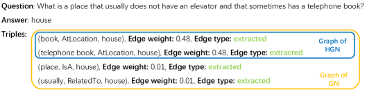
(a) Case I: Unrelated extracted facts are filtered out.

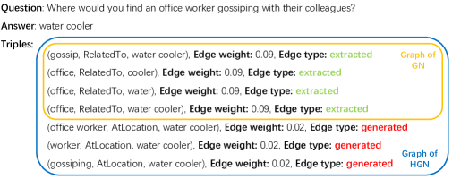
(b) Case II: Helpful generated facts are incorporated.

Figure 5: Representative cases from the development set of CommonsenseQA.

References

- Apperly (2010) Ian Apperly. 2010. Mindreaders: the cognitive basis of” theory of mind”. Psychology Press.
- Banerjee and Baral (2020) Pratyay Banerjee and Chitta Baral. 2020. Knowledge fusion and semantic knowledge ranking for open domain question answering. arXiv preprint arXiv:2004.03101.
- Battaglia et al. (2018) Peter W Battaglia, Jessica B Hamrick, Victor Bapst, Alvaro Sanchez-Gonzalez, Vinicius Zambaldi, Mateusz Malinowski, Andrea Tacchetti, David Raposo, Adam Santoro, Ryan Faulkner, et al. 2018. Relational inductive biases, deep learning, and graph networks. arXiv preprint arXiv:1806.01261.
- Bordes et al. (2013) Antoine Bordes, Nicolas Usunier, Alberto García-Durán, Jason Weston, and Oksana Yakhnenko. 2013. Translating embeddings for modeling multi-relational data. In Advances in Neural Information Processing Systems 26: 27th Annual Conference on Neural Information Processing Systems 2013. Proceedings of a meeting held December 5-8, 2013, Lake Tahoe, Nevada, United States, pages 2787–2795.
- Bosselut and Choi (2019) Antoine Bosselut and Yejin Choi. 2019. Dynamic knowledge graph construction for zero-shot commonsense question answering. arXiv preprint arXiv:1911.03876.
- Bosselut et al. (2019) Antoine Bosselut, Hannah Rashkin, Maarten Sap, Chaitanya Malaviya, Asli Celikyilmaz, and Yejin Choi. 2019. COMET: Commonsense transformers for automatic knowledge graph construction. In Proceedings of the 57th Annual Meeting of the Association for Computational Linguistics, pages 4762–4779, Florence, Italy. Association for Computational Linguistics.
- Chen et al. (2019) Michael Chen, Mike D’Arcy, Alisa Liu, Jared Fernandez, and Doug Downey. 2019. CODAH: An adversarially-authored question answering dataset for common sense. In Proceedings of the 3rd Workshop on Evaluating Vector Space Representations for NLP, pages 63–69, Minneapolis, USA. Association for Computational Linguistics.
- Das et al. (2017) Rajarshi Das, Arvind Neelakantan, David Belanger, and Andrew McCallum. 2017. Chains of reasoning over entities, relations, and text using recurrent neural networks. In Proceedings of the 15th Conference of the European Chapter of the Association for Computational Linguistics: Volume 1, Long Papers, pages 132–141, Valencia, Spain. Association for Computational Linguistics.
- Davison et al. (2019) Joe Davison, Joshua Feldman, and Alexander Rush. 2019. Commonsense knowledge mining from pretrained models. In Proceedings of the 2019 Conference on Empirical Methods in Natural Language Processing and the 9th International Joint Conference on Natural Language Processing (EMNLP-IJCNLP), pages 1173–1178, Hong Kong, China. Association for Computational Linguistics.
- Devlin et al. (2019) Jacob Devlin, Ming-Wei Chang, Kenton Lee, and Kristina Toutanova. 2019. BERT: Pre-training of deep bidirectional transformers for language understanding. In Proceedings of the 2019 Conference of the North American Chapter of the Association for Computational Linguistics: Human Language Technologies, Volume 1 (Long and Short Papers), pages 4171–4186, Minneapolis, Minnesota. Association for Computational Linguistics.
- Feng et al. (2020) Yanlin Feng, Xinyue Chen, Bill Yuchen Lin, Peifeng Wang, Jun Yan, and Xiang Ren. 2020. Scalable multi-hop relational reasoning for knowledge-aware question answering. In Proceedings of the 2020 Conference on Empirical Methods in Natural Language Processing (EMNLP), pages 1295–1309, Online. Association for Computational Linguistics.
- Fleiss (1971) Joseph L Fleiss. 1971. Measuring nominal scale agreement among many raters. Psychological bulletin, 76(5):378.
- Franceschi et al. (2019) Luca Franceschi, Mathias Niepert, Massimiliano Pontil, and Xiao He. 2019. Learning discrete structures for graph neural networks. In Proceedings of the 36th International Conference on Machine Learning, ICML 2019, 9-15 June 2019, Long Beach, California, USA, volume 97 of Proceedings of Machine Learning Research, pages 1972–1982. PMLR.
- Gunning (2018) David Gunning. 2018. Machine common sense concept paper. arXiv preprint arXiv:1810.07528.
- Hu et al. (2019) Ronghang Hu, Anna Rohrbach, Trevor Darrell, and Kate Saenko. 2019. Language-conditioned graph networks for relational reasoning. In 2019 IEEE/CVF International Conference on Computer Vision, ICCV 2019, Seoul, Korea (South), October 27 - November 2, 2019, pages 10293–10302. IEEE.
- Jiang et al. (2019) Bo Jiang, Ziyan Zhang, Doudou Lin, Jin Tang, and Bin Luo. 2019. Semi-supervised learning with graph learning-convolutional networks. In IEEE Conference on Computer Vision and Pattern Recognition, CVPR 2019, Long Beach, CA, USA, June 16-20, 2019, pages 11313–11320. Computer Vision Foundation / IEEE.
- Khashabi et al. (2020) Daniel Khashabi, Sewon Min, Tushar Khot, Ashish Sabharwal, Oyvind Tafjord, Peter Clark, and Hannaneh Hajishirzi. 2020. UNIFIEDQA: Crossing format boundaries with a single QA system. In Findings of the Association for Computational Linguistics: EMNLP 2020, pages 1896–1907, Online. Association for Computational Linguistics.
- Khot et al. (2020) Tushar Khot, Peter Clark, Michal Guerquin, Peter Jansen, and Ashish Sabharwal. 2020. QASC: A dataset for question answering via sentence composition. In The Thirty-Fourth AAAI Conference on Artificial Intelligence, AAAI 2020, The Thirty-Second Innovative Applications of Artificial Intelligence Conference, IAAI 2020, The Tenth AAAI Symposium on Educational Advances in Artificial Intelligence, EAAI 2020, New York, NY, USA, February 7-12, 2020, pages 8082–8090. AAAI Press.
- Kipf et al. (2018) Thomas N. Kipf, Ethan Fetaya, Kuan-Chieh Wang, Max Welling, and Richard S. Zemel. 2018. Neural relational inference for interacting systems. In Proceedings of the 35th International Conference on Machine Learning, ICML 2018, Stockholmsmässan, Stockholm, Sweden, July 10-15, 2018, volume 80 of Proceedings of Machine Learning Research, pages 2693–2702. PMLR.
- Kipf and Welling (2017) Thomas N. Kipf and Max Welling. 2017. Semi-supervised classification with graph convolutional networks. In 5th International Conference on Learning Representations, ICLR 2017, Toulon, France, April 24-26, 2017, Conference Track Proceedings. OpenReview.net.
- Lan et al. (2020) Zhenzhong Lan, Mingda Chen, Sebastian Goodman, Kevin Gimpel, Piyush Sharma, and Radu Soricut. 2020. ALBERT: A lite BERT for self-supervised learning of language representations. In 8th International Conference on Learning Representations, ICLR 2020, Addis Ababa, Ethiopia, April 26-30, 2020. OpenReview.net.
- Lin et al. (2019) Bill Yuchen Lin, Xinyue Chen, Jamin Chen, and Xiang Ren. 2019. KagNet: Knowledge-aware graph networks for commonsense reasoning. In Proceedings of the 2019 Conference on Empirical Methods in Natural Language Processing and the 9th International Joint Conference on Natural Language Processing (EMNLP-IJCNLP), pages 2829–2839, Hong Kong, China. Association for Computational Linguistics.
- Liu and Singh (2004) Hugo Liu and Push Singh. 2004. Conceptnet—a practical commonsense reasoning tool-kit. BT technology journal, 22(4):211–226.
- Liu et al. (2020) Liyuan Liu, Haoming Jiang, Pengcheng He, Weizhu Chen, Xiaodong Liu, Jianfeng Gao, and Jiawei Han. 2020. On the variance of the adaptive learning rate and beyond. In 8th International Conference on Learning Representations, ICLR 2020, Addis Ababa, Ethiopia, April 26-30, 2020. OpenReview.net.
- Liu et al. (2019) Yinhan Liu, Myle Ott, Naman Goyal, Jingfei Du, Mandar Joshi, Danqi Chen, Omer Levy, Mike Lewis, Luke Zettlemoyer, and Veselin Stoyanov. 2019. Roberta: A robustly optimized bert pretraining approach. arXiv preprint arXiv:1907.11692.
- Lv et al. (2020) Shangwen Lv, Daya Guo, Jingjing Xu, Duyu Tang, Nan Duan, Ming Gong, Linjun Shou, Daxin Jiang, Guihong Cao, and Songlin Hu. 2020. Graph-based reasoning over heterogeneous external knowledge for commonsense question answering. In The Thirty-Fourth AAAI Conference on Artificial Intelligence, AAAI 2020, The Thirty-Second Innovative Applications of Artificial Intelligence Conference, IAAI 2020, The Tenth AAAI Symposium on Educational Advances in Artificial Intelligence, EAAI 2020, New York, NY, USA, February 7-12, 2020, pages 8449–8456. AAAI Press.
- Ma et al. (2019) Kaixin Ma, Jonathan Francis, Quanyang Lu, Eric Nyberg, and Alessandro Oltramari. 2019. Towards generalizable neuro-symbolic systems for commonsense question answering. In Proceedings of the First Workshop on Commonsense Inference in Natural Language Processing, pages 22–32, Hong Kong, China. Association for Computational Linguistics.
- Malaviya et al. (2019) Chaitanya Malaviya, Chandra Bhagavatula, Antoine Bosselut, and Yejin Choi. 2019. Exploiting structural and semantic context for commonsense knowledge base completion. arXiv preprint arXiv:1910.02915.
- Marcus (2018) Gary Marcus. 2018. Deep learning: A critical appraisal. arXiv preprint arXiv:1801.00631.
- Mihaylov et al. (2018) Todor Mihaylov, Peter Clark, Tushar Khot, and Ashish Sabharwal. 2018. Can a suit of armor conduct electricity? a new dataset for open book question answering. In Proceedings of the 2018 Conference on Empirical Methods in Natural Language Processing, pages 2381–2391, Brussels, Belgium. Association for Computational Linguistics.
- Neelakantan et al. (2015) Arvind Neelakantan, Benjamin Roth, and Andrew McCallum. 2015. Compositional vector space models for knowledge base completion. In Proceedings of the 53rd Annual Meeting of the Association for Computational Linguistics and the 7th International Joint Conference on Natural Language Processing (Volume 1: Long Papers), pages 156–166, Beijing, China. Association for Computational Linguistics.
- Norcliffe-Brown et al. (2018) Will Norcliffe-Brown, Stathis Vafeias, and Sarah Parisot. 2018. Learning conditioned graph structures for interpretable visual question answering. In Advances in Neural Information Processing Systems 31: Annual Conference on Neural Information Processing Systems 2018, NeurIPS 2018, December 3-8, 2018, Montréal, Canada, pages 8344–8353.
- Petroni et al. (2019) Fabio Petroni, Tim Rocktäschel, Sebastian Riedel, Patrick Lewis, Anton Bakhtin, Yuxiang Wu, and Alexander Miller. 2019. Language models as knowledge bases? In Proceedings of the 2019 Conference on Empirical Methods in Natural Language Processing and the 9th International Joint Conference on Natural Language Processing (EMNLP-IJCNLP), pages 2463–2473, Hong Kong, China. Association for Computational Linguistics.
- Radford et al. (2019) Alec Radford, Jeff Wu, Rewon Child, David Luan, Dario Amodei, and Ilya Sutskever. 2019. Language models are unsupervised multitask learners.
- Raffel et al. (2020) Colin Raffel, Noam Shazeer, Adam Roberts, Katherine Lee, Sharan Narang, Michael Matena, Yanqi Zhou, Wei Li, and Peter J. Liu. 2020. Exploring the limits of transfer learning with a unified text-to-text transformer. Journal of Machine Learning Research, 21(140):1–67.
- Santoro et al. (2017) Adam Santoro, David Raposo, David G. T. Barrett, Mateusz Malinowski, Razvan Pascanu, Peter W. Battaglia, and Tim Lillicrap. 2017. A simple neural network module for relational reasoning. In Advances in Neural Information Processing Systems 30: Annual Conference on Neural Information Processing Systems 2017, December 4-9, 2017, Long Beach, CA, USA, pages 4967–4976.
- Schlichtkrull et al. (2018a) Michael Schlichtkrull, Thomas N Kipf, Peter Bloem, Rianne Van Den Berg, Ivan Titov, and Max Welling. 2018a. Modeling relational data with graph convolutional networks. In European Semantic Web Conference, pages 593–607. Springer.
- Schlichtkrull et al. (2018b) Michael Sejr Schlichtkrull, Thomas N. Kipf, Peter Bloem, Rianne van den Berg, Ivan Titov, and Max Welling. 2018b. Modeling relational data with graph convolutional networks. In The Semantic Web - 15th International Conference, ESWC 2018, Heraklion, Crete, Greece, June 3-7, 2018, Proceedings, volume 10843 of Lecture Notes in Computer Science, pages 593–607. Springer.
- Speer et al. (2017) Robyn Speer, Joshua Chin, and Catherine Havasi. 2017. Conceptnet 5.5: An open multilingual graph of general knowledge. In Proceedings of the Thirty-First AAAI Conference on Artificial Intelligence, February 4-9, 2017, San Francisco, California, USA, pages 4444–4451. AAAI Press.
- Sun et al. (2019) Haitian Sun, Tania Bedrax-Weiss, and William Cohen. 2019. PullNet: Open domain question answering with iterative retrieval on knowledge bases and text. In Proceedings of the 2019 Conference on Empirical Methods in Natural Language Processing and the 9th International Joint Conference on Natural Language Processing (EMNLP-IJCNLP), pages 2380–2390, Hong Kong, China. Association for Computational Linguistics.
- Talmor et al. (2019) Alon Talmor, Jonathan Herzig, Nicholas Lourie, and Jonathan Berant. 2019. CommonsenseQA: A question answering challenge targeting commonsense knowledge. In Proceedings of the 2019 Conference of the North American Chapter of the Association for Computational Linguistics: Human Language Technologies, Volume 1 (Long and Short Papers), pages 4149–4158, Minneapolis, Minnesota. Association for Computational Linguistics.
- Velickovic et al. (2018) Petar Velickovic, Guillem Cucurull, Arantxa Casanova, Adriana Romero, Pietro Liò, and Yoshua Bengio. 2018. Graph attention networks. In 6th International Conference on Learning Representations, ICLR 2018, Vancouver, BC, Canada, April 30 - May 3, 2018, Conference Track Proceedings. OpenReview.net.
- Wang et al. (2020) Peifeng Wang, Nanyun Peng, Filip Ilievski, Pedro Szekely, and Xiang Ren. 2020. Connecting the dots: A knowledgeable path generator for commonsense question answering. In Findings of the Association for Computational Linguistics: EMNLP 2020, pages 4129–4140, Online. Association for Computational Linguistics.
- Wang et al. (2019a) Xiaoyan Wang, Pavan Kapanipathi, Ryan Musa, Mo Yu, Kartik Talamadupula, Ibrahim Abdelaziz, Maria Chang, Achille Fokoue, Bassem Makni, Nicholas Mattei, and Michael Witbrock. 2019a. Improving natural language inference using external knowledge in the science questions domain. In Proceedings of AAAI, pages 7208–7215. AAAI Press.
- Wang et al. (2019b) Xiaoyan Wang, Pavan Kapanipathi, Ryan Musa, Mo Yu, Kartik Talamadupula, Ibrahim Abdelaziz, Maria Chang, Achille Fokoue, Bassem Makni, Nicholas Mattei, et al. 2019b. Improving natural language inference using external knowledge in the science questions domain. In Proceedings of AAAI, volume 33, pages 7208–7215.
- Xu et al. (2020) Yichong Xu, Chenguang Zhu, Ruochen Xu, Yang Liu, Michael Zeng, and Xuedong Huang. 2020. Fusing context into knowledge graph for commonsense reasoning. arXiv preprint arXiv:2012.04808.
- Yasunaga et al. (2021) Michihiro Yasunaga, Hongyu Ren, Antoine Bosselut, Percy Liang, and Jure Leskovec. 2021. QA-GNN: Reasoning with language models and knowledge graphs for question answering. In Proceedings of the 2021 Conference of the North American Chapter of the Association for Computational Linguistics: Human Language Technologies, pages 535–546, Online. Association for Computational Linguistics.
- Yu et al. (2019) Donghan Yu, Ruohong Zhang, Zhengbao Jiang, Yuexin Wu, and Yiming Yang. 2019. Graph-revised convolutional network. In Proceedings of ECML-PKDD.