On Transferability of Bias Mitigation Effects in Language
Model Fine-Tuning

Abstract

Fine-tuned language models have been shown to exhibit biases against protected groups in a host of modeling tasks such as text classification and coreference resolution. Previous works focus on detecting these biases, reducing bias in data representations, and using auxiliary training objectives to mitigate bias during fine-tuning. Although these techniques achieve bias reduction for the task and domain at hand, the effects of bias mitigation may not directly transfer to new tasks, requiring additional data collection and customized annotation of sensitive attributes, and re-evaluation of appropriate fairness metrics. We explore the feasibility and benefits of upstream bias mitigation (UBM) for reducing bias on downstream tasks, by first applying bias mitigation to an upstream model through fine-tuning and subsequently using it for downstream fine-tuning. We find, in extensive experiments across hate speech detection, toxicity detection, occupation prediction, and coreference resolution tasks over various bias factors, that the effects of UBM are indeed transferable to new downstream tasks or domains via fine-tuning, creating less biased downstream models than directly fine-tuning on the downstream task or transferring from a vanilla upstream model. Though challenges remain, we show that UBM promises more efficient and accessible bias mitigation in LM fine-tuning.

1 Introduction

The practice of fine-tuning pretrained language models (PTLMs or LMs), such as BERT (Devlin et al., 2019), has improved prediction performance in a wide range of NLP tasks. However, fine-tuned LMs may exhibit biases against certain protected groups (e.g., gender and ethnic minorities), as models may learn to associate certain features with positive or negative labels spuriously (Dixon et al., 2018), or propagate bias encoded in PTLMs to downstream classifiers (Caliskan et al., 2017; Bolukbasi et al., 2016). Among many examples, Kurita et al. (2019) demonstrates gender-bias in the pronoun resolution task when models are trained using BERT embeddings, and Kennedy et al. (2020) shows that hate speech classifiers fine-tuned from BERT result in more frequent false positive predictions for certain group identifier mentions (e.g., “muslim”, “black”).

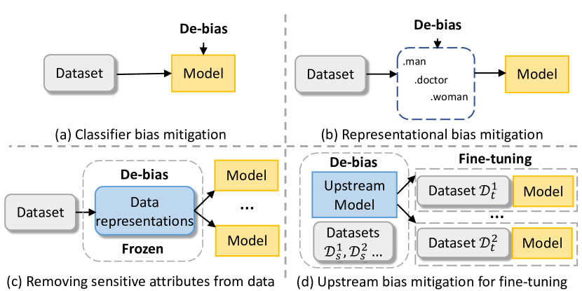
Figure 1: Comparison between the focus of our study (d) and previous works (a,b,c). We study the viability of obtaining an upstream model that could reduce bias in a number of downstream classifiers when fine-tuned.

Approaches for bias mitigation are mostly applied during fine-tuning to reduce bias in a specific downstream task or dataset (Park et al., 2018; Zhang et al., 2018; Beutel et al., 2017) (see Fig. 1 (a)). For example, data augmentation approaches reduce the influence of spurious features in the original dataset (Dixon et al., 2018; Zhao et al., 2018; Park et al., 2018), and adversarial learning approaches generate debiased data representations that are exclusive to the downstream model (Kumar et al., 2019; Zhang et al., 2018). These techniques act on biases particular to the given dataset, domain, or task, and require new bias mitigation when switching to a new downstream task or dataset. This can require auxiliary training objectives, the definition of task-specific fairness metrics, the annotation of bias attributes (e.g., identifying African American Vernacular English), and the collection of users’ demographic data. These drawbacks make bias mitigation inaccessible to the growing community, fine-tuning LMs to new datasets and tasks.

In contrast, we investigate initially mitigating bias while fine-tuning an “upstream” model in one or more upstream datasets, and subsequently achieving reduced bias when fine-tuning for downstream applications (Fig. 1 (d)), so that bias mitigation is no longer required in downstream training. Similar to transfer learning for enhancing predictive performance in common setups Pan and Yang (2010); Dai and Le (2015), we suggest that LMs that undergo bias mitigation acquire inductive bias that is helpful for reducing harmful biases when fine-tuned on new domains and tasks. In four tasks with known bias factors — hate speech detection, toxicity detection, occupation prediction from short bios, and coreference resolution — we explore whether upstream bias mitigation of a LM followed by downstream fine-tuning reduces bias for the downstream model. Though previous work has addressed biases in frozen PTLM or word embeddings Bolukbasi et al. (2016); Zhou et al. (2019); Bhardwaj et al. (2020); Liang et al. (2020); Ravfogel et al. (2020), for example by measuring associations between gender and occupations in an embedding space, they do not study their effect on downstream classifiers (Fig. 1 (b)), while some of them study the effects while keeping the embeddings frozen Zhao et al. (2019); Kurita et al. (2019); Prost et al. (2019). Bias in these frozen representations can also be directly corrected by removing associations between feature and sensitive attributes Elazar and Goldberg (2018); Madras et al. (2018) (Fig. 1 (c)), but this does not allow predictions to be generated for new data.

Our experiments address the following research questions: (a) whether mitigating a single bias factor in the upstream stage is maintained when fine-tuning on new examples from the same domain and task, (b) whether transfer is viable when the downstream domains and tasks are different from the upstream model, and (c) whether we can address multiple kinds of bias with a single upstream model. We perform these experiments under a generic transfer learning framework, noted as Upstream Bias Mitigation (UBM) for Downstream Fine-Tuning for convenience, which consists of two stages: first, in the upstream bias mitigation stage, a LM is fine-tuned with bias mitigation objectives on one or several “upstream” tasks, and subsequently the classification layer is re-initialized; then, in the downstream fine-tuning stage the encoder from the upstream model, jointly with the new classification layer, are again fine-tuned on a downstream task without additional bias mitigation steps. Using six datasets with previously recognized bias factors, our analysis show overall positive results for the questions above; still, there are challenges remaining to stabilize the results of bias mitigation in challenging setups, e.g., the multi-bias factor setting.

Our contributions are summarized as follows: (1) we propose a new research direction for mitigating bias in fine-tuned models; (2) we perform extensive experiments to study the viability of the upstream bias mitigation framework in various settings; (3) we demonstrate the effectiveness of this research direction, motivating further improvements, tests, and applications.

2 Exploring the Transferability of Bias Mitigation Effects

We consider biases against protected groups in classifiers fined-tuned from LMs. In our present analysis, bias is defined as disparate model performance on different subsets of data which are associated with different demographic groups (e.g., instances that mention or are generated by different social groups) (Blodgett et al., 2020). Our evaluation of bias aligns with the definition of equalized odds and equal opportunities Hardt et al. (2016) in previous works of fairness in machine learning.

Here, we first outline our experimental setup for exploring the transferability of bias mitigation effects, in which we detail the process of applying UBM and pose three key research questions (section 2.1). We follow by introducing the bias factors studied and the corresponding classification tasks and datasets (section 2.2), and our evaluation protocols and metrics (section 2.3).

2.1 Experiment Setups of UBM

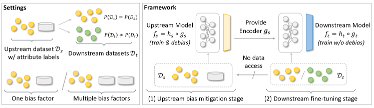
Figure 2: Experiment setups to study Upstream Bias Mitigation (UBM) for Downstream Fine-Tuning. We consider the settings with the same or different upstream and downstream domains and tasks, while addressing one or more bias factors (e.g., both dialect bias and gender bias). The framework consists of two stages: (1) an upstream (source) model $f_{s}=h_{s}\circ g_{s}$ is trained with bias mitigation algorithms and (2) the encoder $g_{s}$ is transferred to the downstream (target) model $f_{t}$ for fine-tuning.

Our goal is to evaluate the transferability of bias mitigation effects for one or multiple bias factors in downstream fine-tuned models. We follow an Upstream Bias Mitigation (UBM) for Downstream Fine-Tuning procedure, pictured in Figure 2. First, in the Upstream Bias Mitigation phase, an upstream (source) model $f_{s}=h_{s}\circ g_{s}$, composed of a text encoder $g_{s}$ and a classifier head $h_{s}$, is trained on one or more upstream datasets $\mathcal{D}_{s}$ with bias mitigation algorithms. The encoder $g_{s}$ is to be transferred to downstream (target) domains and tasks while the classifier head $h_{s}$ is discarded. Then, in the Downstream Fine-Tuning phase, the downstream model $f_{t}=h_{t}\circ g_{t}$ utilizes $g_{s}$ to initialize the encoder weights and is fine-tuned for prediction performance without bias mitigation approaches on downstream datasets $\mathcal{D}_{t}$.

This UBM process is applied in three settings, summarized below, which each contribute to evaluating the transferability of bias mitigation effects.

1. Fine-Tuning on the Same Distribution. In the simplest setting, we fine-tune the downstream model over new examples from the same data distribution as the upstream model. In practice, each dataset is split into two halves, with one used for upstream bias mitigation and the other for downstream fine-tuning.

2. Cross-Domain and Cross-Task Fine-Tuning. Similar to how LMs are fine-tuned for various tasks and domains, in a more practical setup, we test whether transfer of bias mitigation effects is viable across domains and tasks. To achieve this, we apply bias mitigation while fine-tuning a LM on one dataset and perform fine-tuning on another.

3. Multiple Bias Factors. In the most challenging setup, we train a single upstream model to address multiple bias factors (e.g., both dialect bias and gender bias). Such upstream models can be trained with multi-task learning (i.e., jointly training over multiple datasets with shared encoder $g$ but different classifier heads $h$) while mitigating multiple kinds of bias. Subsequently, the resulting upstream model is transferred to downstream models as before. This is a key test of UBM’s viability for widespread application.

2.2 Bias Factors and Datasets

To ensure our analysis holds true for a variety of domains, tasks, and bias factors, we experiment with three different bias factors studied in previous research along with six different datasets (also summarized in Table 1), described below.

Group Identifier Bias. This bias refers to higher false positive rates of hate speech predictions for sentences containing specific group identifiers, which is harmful to protected groups by misclassifying innocuous text (e.g., “I am a Muslim”) as hate speech. We include two datasets for study, namely the Gab Hate Corpus (GHC; Kennedy et al., 2018) and the Stormfront corpus (de Gibert et al., 2018). Both datasets contain binary labels for hate and non-hate instances, though with differences in the labeling schemas and domains.

Dataset	Prediction Task	Bias
GHC Kennedy et al. (2018)	Hate	Group Identifier
Stormfront de Gibert et al. (2018)	Hate	Group Identifier
DWMW Davidson et al. (2017)	Toxicity	AAVE Dialect
FDCL Founta et al. (2018)	Toxicity	AAVE Dialect
BiasBios De-Arteaga et al. (2019)	Occupation	Gender Stereotyping
OntoNotes 5.0 Weischedel et al. (2013)	Coreference	Gender Stereotyping

Table 1: Summary of tasks and bias included for study.

AAVE Dialect Bias. Sap et al. (2019) show that offensive and hate speech classifiers yield a higher false positive rate on text written in African American Vernacular English (AAVE). This bias brings significant harm to the communities that uses AAVE, for example, by leading to the disproportionate removal of the text written in AAVE in social media platforms (Blodgett et al., 2020). We include two datasets for study: FDCL (Founta et al., 2018) and DWMW (Davidson et al., 2017). In both datasets, we treat abusive, hateful and spam together as harmful outcomes (i.e., false positives for each are harmful) to compute false positive rates. Following Sap et al. (2019), we use an off-the-shelf AAVE dialect predictor (Blodgett et al., 2016) to identify examples written in AAVE.

Gender Stereotypical Bias.  Zhao et al. (2018) summarize a list of occupations that are prone to be stereotyped in practice, leading to coreference resolutions models and occupation prediction models having biases in performance in pro- and anti-stereotypical instances when trained on short bios. We train the coreference resolution model on the OntoNotes 5.0 dataset Weischedel et al. (2013) and the occupation classifier on the BiasBios De-Arteaga et al. (2019) dataset.

2.3 Evaluation Protocol and Metrics

We evaluate the overall performance of the models on downstream tasks along with appropriate bias metrics for each bias factor, analyzed for each dataset and task in previous works. We expect UBM to minimally affect classification performance while improving on bias metrics.

Classification Performance. We report in-domain F1 scores for GHC, Stormfront, OntoNotes 5.0, and accuracy scores for FDCL, DWMW and BiasBios. Following Zhang et al. (2018), for hate speech detection and toxicity detection datasets, we use the equal error rate (EER) threshold for prediction.

Group Identifier Bias Metrics. To evaluate group identifier bias, we evaluate false positive rate (FPR) differences, noted as FPRD, between examples mentioning one of 25 group identifiers provided by Kennedy et al. (2020) and the overall FPR. In addition, we followed Kennedy et al. (2020) in using a New York Times articles (NYT) corpus of 25$k$ non-hate sentences, each mentioning one of 25 group identifiers. This corpus specifically provides an opportunity to measure FPR—reported as (NYT Acc.), equivalent to $1-$FPR. Additionally, following the evaluation protocol of Dixon et al. (2018) and Zhang et al. (2020), we incorporate the Identity Phrase Templates Test Sets (reported as IPTTS), which consists of $77k$ hate and non-hate examples mentioning group identifiers, generated with templates. Following these works, for IPTTS we compute FPRD as $\sum_{z}|\mathrm{FPR}_{z}-\mathrm{FPR}_{overall}|$, where $\textrm{FPR}_{z}$ is false positive rate on sentences with the group identifier $z$, and $\mathrm{FPR}_{overall}$ is the overall false positive rate.

AAVE Dialect Bias Metrics. Given the sparsity of AAVE examples in the datasets and the noisy outputs of AAVE classifier (Blodgett et al., 2016), we expect the in-domain FPRD metrics to be noisy. Therefore, following Xia et al. (2020), we incorporate the BROD (Blodgett et al., 2016) dataset, which is a large unlabeled collection of Twitter posts written in l. Since in practice only a small portion of texts are toxic or spam, we treat all examples from BROD as normal, and report the accuracy (which equals $1-$FPR) on the dataset.

Gender Stereotype Metrics. We employ the WinoBias Zhao et al. (2018) dataset which provides opportunities to evaluate models on pro-stereotypical and anti-stereotypical coreference examples. We report the differences in F1 (F1-Diff) on two subsets of data. On occupation prediction, following Ravfogel et al. (2020), we report mean differences of true positive rate (TPR) differences in predicting each occupation for men and women.

3 Method

Here, we detail the particular bias mitigation algorithms used for implementing UBM, as well as the other baselines used for verifying the transferability of bias mitigation effects.

3.1 Implementations of UBM

We implement UBM with two different bias mitigation algorithms in the upstream bias mitigation phase: explanation regularization (Kennedy et al., 2020), and adversarial de-biasing (Zhang et al., 2018; Madras et al., 2018; Xia et al., 2020), denoted here as UBM_reg and UBM_adv, respectively.

UBM with Explanation Regularization. Explanation regularization reduces importance placed on spurious surface patterns (i.e., words or phrases) during upstream model training. We apply UBM_reg to group identifier and AAVE dialect bias, where the set of spurious patterns are group identifiers and the most frequent words, from statistics of the dataset, used by AAVE speakers; we find explanation regularization not effective for gender bias. The importance of a surface pattern $w\in\mathcal{W}$ in the input ${\mathbf{x}}$, noted as $\phi(w,{\mathbf{x}})$ is measured as the model prediction change when it is removed. The model is trained by optimizing the main learning objective $\ell$ while penalizing importance attributed to patterns $w\in\mathcal{W}$ that exist in the input ${\mathbf{x}}$.

$$\min_{f}\quad\ell_{c}+\alpha\sum_{w\in{\mathbf{x}}\cap\mathcal{W}}||\phi(w,{\mathbf{x}})||^{2},$$ (1)

where $\alpha$ is a trade-off hyperparameter.

UBM  with Adversarial De-biasing. In UBM_adv, the upstream model is trained with adversarial de-biasing techniques, so that sensitive attributes related to bias (e.g., the dialect of the sentence or the gender referenced in the sentence) cannot be predicted from the hidden representations ${\mathbf{z}}$ given by the encoder $g$. During training, an adversarial classifier head $h^{adv}$ is built upon the encoder and trained to predict sensitive attributes, while the encoder is optimized to prevent the adversarial classifier from success. Formally, the optimization objective is written as,

$$\min_{g,h}\max_{h_{adv}}\quad\ell_{c}+\ell_{adv}(h_{adv}\circ g({\mathbf{x}}),a),$$ (2)

where $a$ notes the ground truth sensitive attribute, and $\ell_{adv}$ is the cross entropy loss between the predicted sensitive attribute and the ground truth sensitive attribute.

As mentioned in Sec. 2.1, upstream models can be trained to mitigate multiple bias factors with multi-task learning on multiple datasets. We separately apply bias mitigation algorithms for each dataset (sharing the same encoder) and note the algorithms applied in the subscript (e.g., UBM_reg+adv).

3.2 Other Baselines

We compare UBM with two families of methods.

Methods without Bias Mitigation. Two types of models were evaluated that did not address bias. First, the Vanilla model is a downstream classifier directly fine-tuned on downstream task from a LM (e.g., RoBERTa). Second, Van-Transfer is fine-tuned on upstream datasets without bias mitigation and fine-tuned on downstream datasets.

Downstream Bias Mitigation. For reference, we show the results of directly applying explanation regularization, noted as Expl. Reg., or adversarial de-biasing, noted as Adv. Learning, during down-stream fine-tuning. In most cases, mitigating bias in downstream classifier should be the most effective way to reduce bias, though this is not always feasible in practice for reasons discussed above.

We also consider two simple baselines that could reduce bias in downstream models via heuristics. Emb. Zero zeros out the word embedding of spurious surface patterns (using the same word list as explanation regularization) in PTLMs before fine-tuning. We also include Emb. Zero. Trans, which zeros out embeddings of spurious surface patterns before fine-tuning from an upstream model. The method does not apply to cases where surface patterns related to bias (e.g., gendered pronouns) are crucial for prediction, e.g., coreference resolution.

4 Results

	GHC B
Metrics	In-domain F1 ($\uparrow$)	In-domain FPRD ($\downarrow$)	IPTTS FPRD ($\downarrow$)	NYT Acc ($\uparrow$)
	Non-Transfer (GHC . B)
Vanilla	37.91 $\pm$ 2.5	35.64 $\pm$ 2.2	21.50 $\pm$ 2.8	68.55 $\pm$ 20
Expl. Reg.	38.09 $\pm$ 2.7	18.68 $\pm$ 0.3	4.82 $\pm$ 1.1	84.05 $\pm$ 3.0
	GHC . A $\to$ GHC . B
Van. Transfer	42.41 $\pm$ 1.0	37.44 $\pm$ 1.5	17.67 $\pm$ 2.1	75.35 $\pm$ 4.2
UBMReg	43.79 $\pm$ 1.9	34.34 $\pm$ 3.1	10.02 $\pm$ 1.1	81.40 $\pm$ 1.4

Table 2: Same-domain and task UBM with a single bias factor. The source datasets are noted before arrow $(\rightarrow)$. All metrics except In-domain F1 measure bias. See Table 6 in Appendix for complete results.

Downstream dataset	GHC				Stormfront				DWMW		OntoNotes 5.0
Metrics	In-domain F1 ($\uparrow$)	In-domain FPRD ($\downarrow$)	IPTTS FPRD ($\downarrow$)	NYT Acc ($\uparrow$)	In-domain F1 ($\uparrow$)	In-domain FPRD ($\downarrow$)	IPTTS FPRD ($\downarrow$)	NYT Acc ($\uparrow$)	In-domain Acc. ($\uparrow$)	BROD Acc. ($\uparrow$)	In-domain F1 ($\uparrow$)	Winobias F1-Diff ($\downarrow$)
	Non-Transfer (GHC)				Non-Transfer (Stormfront)				Non-Transfer (DWMW)		Non-Transfer (OntoNotes 5.0)
Vanilla	49.60 $\pm$ 1.0	46.43 $\pm$ 2.5	20.01 $\pm$ 5.7	72.08 $\pm$ 7.3	53.74 $\pm$ 2.8	18.09 $\pm$ 2.7	11.51 $\pm$ 5.1	73.06 $\pm$ 10	91.46 $\pm$ 0.1	78.77 $\pm$ 0.3	76.53 $\pm$ 0.2	8.04 $\pm$ 0.5
Emb. Zero	43.76 $\pm$ 0.7	38.31 $\pm$ 2.0	11.95 $\pm$ 2.7	83.21 $\pm$ 5.2	49.97 $\pm$ 0.6	18.80 $\pm$ 2.0	8.20 $\pm$ 0.3	70.15 $\pm$ 4.4	90.59 $\pm$ 0.1	62.37 $\pm$ 0.4
Expl. Reg.	43.37 $\pm$ 1.8	29.29 $\pm$ 1.2	4.2 $\pm$ 1.6	81.22 $\pm$ 11	51.53 $\pm$ 1.1	13.43 $\pm$ 1.5	3.80 $\pm$ 0.4	83.73 $\pm$ 8.0	91.38 $\pm$ 0.1	76.61 $\pm$ 1.5
Adv. Learning									91.11 $\pm$ 0.3	77.53 $\pm$ 0.9
	Stf. $\to$ GHC				GHC $\to$ Stf.				FDCL $\to$ DWMW		BiasBios $\to$ OntoNotes 5.0
Van-Transfer	47.83 $\pm$ 2.1	47.51 $\pm$ 4.6	14.00 $\pm$ 0.8	66.71 $\pm$ 10.6	55.79 $\pm$ 1.3	17.83 $\pm$ 2.2	8.26 $\pm$ 2.5	76.98 $\pm$ 1.1	91.27 $\pm$ 0.2	78.98 $\pm$ 1.1	76.65 $\pm$ 0.3	10.54 $\pm$ 0.7
Emb. Zero. Trans.	44.51 $\pm$ 0.5	40.92 $\pm$ 4.2	12.91 $\pm$ 0.2	80.11 $\pm$ 1.2	52.98 $\pm$ 0.6	16.35 $\pm$ 0.9	8.04 $\pm$ 2.1	81.11 $\pm$ 1.9	91.53 $\pm$ 0.0	81.01 $\pm$ 0.9
UBMReg	49.94 $\pm$ 1.0	42.71 $\pm$ 3.8	12.23 $\pm$ 3.3	75.34 $\pm$ 4.8	56.43 $\pm$ 0.6	18.03 $\pm$ 2.5	6.86 $\pm$ 1.1	81.18 $\pm$ 1.1	91.39 $\pm$ 0.0	80.27 $\pm$ 0.2
UBMAdv									91.20 $\pm$ 0.0	81.24 $\pm$ 0.2	76.34 $\pm$ 0.2	9.27 $\pm$ 1.4

Table 3: Cross-domain and task UBM with a single bias factor. The source datasets are noted before arrow $(\rightarrow)$. All metrics except In-domain F1 or In-domain Accuracy measures bias. The preferred outcomes for each metric are marked with arrows. The main comparators of UBM are Vanilla, Van-Transfer, Emb. Zero, and Emb. Zero. Trans that do not perform downstream bias mitigation. We see UBM maintains in-domain prediction performance while overall reduces bias. Results of Adv. Learning and UBM_Adv on GHC, Stf. are not included because applying adversarial de-biasing to reduce group identifier bias yields degenerated classifiers.

In this section, we present the results of UBM in three settings following the order in Sec. 2.1: transferring to the same data distribution, transferring to different data distributions, transferring from an upstream model with bias mitigation for multiple bias factors. We follow these main analyses with an investigation of the impact of freezing encoder weights before downstream fine-tuning, and lastly with a brief exploration of how UBM’s positive results are achieved.

Implementation Details. In all experiments reported on below, models are initially fine-tuned from RoBERTa-base. The upstream model is trained for a fixed number of epochs and the checkpoint with the best prediction performance is transferred to the downstream model. See Appendix for more implementation details. We use $\mathcal{D}_{s}\to\mathcal{D}_{t}$ as the transfer notation, in which upstream and downstream datasets are respectively represented in the left and right-hand side of the arrow.

4.1 UBM with the Same Data Distribution

We first briefly show the results when the downstream model sees new, unseen samples from the same data distribution as the upstream model. In this controlled setting, we isolate and test the basic viability of UBM, which requires that information from the upstream model is retained during downstream fine-tuning. GHC, Stormfront, FDCL and BiasBios were partitioned into two subsets with equal size, noted as subsets A and B of corresponding datasets, to train the upstream and downstream models respectively.

Table 2 presents the results for mitigating group identifier bias in the GHC. We see an overall bias reduction, via UBM, by comparing with Vanilla training and Van-Transfer. We include full results and discussions for this simple setting in Appendix.

4.2 Cross-domain and Task UBM

Following the result that UBM is effective in the same-domain setting, we now move to analyzing cross-domain settings in greater depth. For hate speech classification, we perform transfer learning from GHC to Stormfront and from Stormfront to GHC; and for toxicity classification, we perform transfer learning from FDCL to DWMW. We also perform transfer learning from BiasBios (occupation prediction) to OntoNotes 5.0 (coreference resolution). Table 3 shows the results of cross-domain and task transfer learning and non-transfer baselines. Our findings are summarized below.

UBM can reduce bias in different target domains and tasks compared to fine-tuning without bias mitigation. The results of cross-domain and task transfer learning (i.e., Stf.$\to$GHC, GHC$\to$Stf., FDCL$\to$DWMW), show that transferring from a less biased upstream model (UBM_Reg and UBM_Adv) leads to better downstream bias mitigation compared to directly training without bias mitigation in the target domain (Vanilla). Meanwhile, the in-domain classification performance has improved (on GHC and Stormfront) or been preserved (on DWMW). It is notable that directly mitigating bias (Expl. Reg., Adv. Learning) on DWMW is not effective, which is previously observed by Xia et al. (2020), while transferring from FDCL is successful.

There are exceptions where UBM fails to reduce bias. We see the in-domain FPRD on Stormfront does not improve; however, as discussed in our metrics section, the in-domain FPRD is computed over a much smaller set of examples compared to NYT and IPTTS datasets, and is thus less reliable. UBM does not reduce bias compared to Vanilla training on OntoNotes 5.0, but achieves less bias compared to Van-Transfer. This result confirms the effect of bias mitigation in upstream models, but the transfer learning itself has increased the bias.

Comparison with Emb. Zero and Emb. Zero. Trans. We find two alternative methods, Emb. Zero and Emb. Zero Trans, also reduce bias on some of the datasets. On GHC, Emb. Zero achieves an in-domain FPRD and IPTTS-FPRD lower than UBM. However, it comes with clear drop of in-domain classification performance.

Bias Factor	Group Identifier Bias				AAVE Dialect Bias		Gender Stereotypical Bias
Metrics	In-domain F1 ($\uparrow$)	In-domain FPRD ($\downarrow$)	IPTTS FPRD ($\downarrow$)	NYT Acc ($\uparrow$)	In-domain F1 ($\uparrow$)	BROD Acc. ($\uparrow$)	In-domain F1 ($\uparrow$)	Winobias F1-Diff ($\downarrow$)
Upstream model	Stormfront + FDCL
Downstream model	GHC				DWMW
Van-Transfer	49.71 $\pm$ 0.3 0.05emcol1$\nearrow$	45.84 $\pm$ 3.8 0.05emcol3$\searrow$	12.43 $\pm$ 2.5 0.05emcol3$\searrow$	72.37 $\pm$ 7.4 0.05emcol1$\nearrow$	91.64 $\pm$ 0.2 0.05emcol1$\nearrow$	81.12 $\pm$ 0.1 0.05emcol1$\nearrow$
UBMReg,Reg	50.21 $\pm$ 1.4 0.05emcol1$\nearrow$	47.63 $\pm$ 0.7 0.05emwhite$\rightarrow$	12.29 $\pm$ 2.7 0.05emcol3$\searrow$	68.44 $\pm$ 8.6 0.05emwhite$\rightarrow$	91.66 $\pm$ 0.2 0.05emcol1$\nearrow$	80.05 $\pm$ 0.1 0.05emcol1$\nearrow$
UBMReg,Adv	49.89 $\pm$ 1.7 0.05emcol1$\nearrow$	47.85 $\pm$ 1.2 0.05emwhite$\rightarrow$	21.25 $\pm$ 2.0 0.05emwhite$\rightarrow$	65.78 $\pm$ 5.7 0.05emwhite$\rightarrow$	91.55 $\pm$ 0.2 0.05emcol1$\nearrow$	81.14 $\pm$ 1.5 0.05emcol1$\nearrow$
Upstream Model	GHC + FDCL
Downstream Model	Stormfront				DWMW
Van-Transfer	56.78 $\pm$ 1.6 0.05emcol1$\nearrow$	14.26 $\pm$ 0.8 0.05emcol3$\searrow$	11.04 $\pm$ 0.7 0.05emcol3$\searrow$	77.06 $\pm$ 5.1 0.05emcol1$\nearrow$	91.65 $\pm$ 0.1 0.05emcol1$\nearrow$	80.98 $\pm$ 0.4 0.05emcol1$\nearrow$
UBMReg,Reg	53.87 $\pm$ 1.2 0.05emcol1$\nearrow$	15.92 $\pm$ 1.2 0.05emcol3$\searrow$	8.40 $\pm$ 1.4 0.05emcol3$\searrow$	83.71 $\pm$ 3.2 0.05emcol1$\nearrow$	91.79 $\pm$ 0.4 0.05emcol1$\nearrow$	81.36 $\pm$ 0.8 0.05emcol1$\nearrow$
UBMReg,Adv	53.63 $\pm$ 0.7 0.05emwhite$\rightarrow$	15.52 $\pm$ 2.2 0.05emcol3$\searrow$	8.90 $\pm$ 1.6 0.05emcol3$\searrow$	84.87 $\pm$ 1.1 0.05emcol1$\nearrow$	91.33 $\pm$ 0.1 0.05emwhite$\rightarrow$	81.09 $\pm$ 0.4 0.05emcol1$\nearrow$
Upstream Model	GHC + FDCL + BiasBios
Downstream Model	Stormfront				DWMW		OntoNotes 5.0
Van-Transfer	55.47 $\pm$ 0.7 0.05emcol1$\nearrow$	16.74 $\pm$ 1.5 0.05emcol3$\searrow$	12.19 $\pm$ 0.7 0.05emcol3$\searrow$	64.15 $\pm$ 6.5 0.05emwhite$\rightarrow$	91.58 $\pm$ 0.1 0.05emcol1$\nearrow$	80.74 $\pm$ 0.3 0.05emcol1$\nearrow$	73.64 $\pm$ 0.3 0.05emwhite$\rightarrow$	9.91 $\pm$ 0.2 0.05emwhite$\rightarrow$
UBMReg,Reg,Adv	52.59 $\pm$ 0.5 0.05emwhite$\rightarrow$	21.17 $\pm$ 2.0 0.05emwhite$\rightarrow$	9.99 $\pm$ 2.8 0.05emcol3$\searrow$	74.58 $\pm$ 4.9 0.05emcol1$\nearrow$	91.64 $\pm$ 0.3 0.05emcol1$\nearrow$	81.07 $\pm$ 0.4 0.05emcol1$\nearrow$	75.68 0.05emwhite$\rightarrow$	4.93 0.05emcol3$\searrow$
UBMReg,Adv,Adv	52.85 $\pm$ 0.9 0.05emwhite$\rightarrow$	18.55 $\pm$ 5.8 0.05emwhite$\rightarrow$	13.15 $\pm$ 3.7 0.05emcol3$\searrow$	70.00 $\pm$ 5.8 0.05emwhite$\rightarrow$	91.50 $\pm$ 0.1 0.05emcol1$\nearrow$	81.08 $\pm$ 0.3 0.05emcol1$\nearrow$	76.01 $\pm$ 0.4 0.05emwhite$\rightarrow$	8.67 $\pm$ 0.7 0.05emwhite$\rightarrow$

Table 4: Dealing with multiple bias factors with a single upstream model with UBM. We test three combination of upstream datasets, namely Stormfront + FDCL, GHC + FDCL, and GHC + FDCL + BiasBios, in reducing two or three bias factors. 0.05emcol1$\nearrow$ and 0.05emcol3$\searrow$ show whether the metrics has increased or decreased (both imply improvement) compared to non-transfer Vanilla training in Table 3.

Metrics	In-domain Acc. ($\uparrow$)	In-domain FPRD ($\downarrow$)	IPTTS FPRD ($\downarrow$)	NYT Acc. ($\uparrow$)	In-domain Acc. ($\uparrow$)	BROD Acc. ($\uparrow$)
	Stf. $\to$ GHC, UBMReg				FDCL $\to$ DWMW, UBMAdv
Freeze	45.42	37.71	7.82	84.45	83.25	64.80
$\ell^{2}$-sp	49.31	47.03	14.24	71.88	91.38	79.95
Fine-tune	49.94	42.71	12.23	75.34	91.20	81.24
	GHC $\to$ Stf. UBMReg
Freeze	47.32	25.02	8.24	64.60
$\ell^{2}$-sp	55.80	19.75	6.72	80.42
Fine-tune	56.43	18.03	6.86	81.18

Table 5: UBM while keeping the encoder frozen (Freeze), discouraging parameter changes ($\ell^{2}$-sp), or standard fine-tuning (Fine-tune). We see weight freezing and $\ell^{2}$-sp overall do not improve over simple fine-tuning on Stf. $\to$ GHC and FDCL $\to$ DWMW.

4.3 Mitigating Multiple Bias Factors

Having observed an overall positive effect of UBM across domains and tasks, next we present the results of experiments on mitigating multiple bias factors with a single upstream model. This involves training an upstream model with multiple bias mitigation objectives across multiple datasets, followed by fine-tuning on a single dataset without bias mitigation. We test three combinations of datasets. First, a multi-task model is trained to jointly mitigate group identifier bias and AAVE dialect bias using GHC and FDCL (GHC + FDCL), and transferred to Stormfront and DWMW. Next, a model is similarly trained jointly on group identifier and AAVE biases on and Stormfront and FDCL (Stf. + FDCL) and transferred to GHC and DWMW. Lastly, models were trained over source datasets GHC, FDCL, BiasBios (GHC+FDCL+BiasBios) to mitigate all three bias factors, and transferred to Stormfront, DWMW, and OntoNotes. The results are shown in Table 4.

Comparison to Single-Dataset Vanilla Baselines. As a basic measure of bias mitigation success, we compare multi-dataset models’ results with single-dataset Vanilla training and Van-Transfer. We see UBM with GHC + FDCL successfully reduces both group identifier bias and AAVE dialect bias in downstream models. UBM with GHC + FDCL + BiasBios also successfully reduces group identifier bias in terms of IPTTS, FPRD (which is the most reliable metrics of bias given its large size), and AAVE bias. It also reduces gender stereotypical bias compared to Van-Transfer in some experimental runs, but in an unstable manner, demonstrated by the large variance of F1-Diff and degenerated runs of UBM_Reg,Reg,Adv.

Results of UBM on Stf. + FDCL are less promising. We find UBM_Reg,Adv,Adv is not successful in reducing group identifier bias. UBM_Reg,Reg,Adv could reduce bias on IPTTS-FPRD, but does not improve other metrics. Notably, UBM on Stf. + FDCL clearly underperform UBM on Stf. only.

UBM_Reg versus UBM_Adv. Empirically, we find using explanation regularization on FDCL (UBM_reg,reg, UBM_reg,reg,adv) instead of adversarial learning (UBM_reg,adv, UBM_reg,adv,adv) consistently improves bias mitigation performance on other bias factors.

Takeaways. Our results show it is possible to reduce multiple bias factors via UBM. However, we have shown that these effects are not automatic for each new dataset added to upstream models for multi-task bias mitigation.

4.4 Freezing or Regularizing Model Weights

In the experiments above, we have shown that the effect of mitigating bias is partially preserved with simple fine-tuning. Next, we study whether freezing the encoders or discouraging their weight changes improves bias mitigation in the target domain, as they intuitively try to retain effect of bias mitigation. However, we find a counter-intuitive result: these approaches typically do not achieve reduced downstream bias, and in fact reduce in-domain classification performance. Table 5 shows the results when we keep the weights frozen (Freeze), discouraging weights from changing with $\ell^{2}$-sp regularizer (Li et al., 2018, details in appendix), or standard fine-tuning (fine-tune). In Stf. $\to$ GHC, freezing the weights contributed to reducing the bias, while $\ell^{2}$-sp failed to help. In GHC $\to$ Stf and FDCL $\to$ DWMW, freezing the weights and $\ell^{2}$-sp both increased the bias. A possible reason is that by freezing the encoder, we reduce its expressive power. As a result, the encoder is prone to capture simple but spurious correlations.

4.5 Investigating Why UBM Reduces Bias

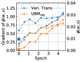
(a)

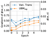
(b)

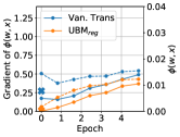
(c)

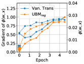
(d)

Figure 3: Gradient of importance attribution on group identifiers $\phi(w,{\mathbf{x}})$ over time (in solid lines) and the corresponding values of $\phi(w,{\mathbf{x}})$ (in dash lines) during downstream fine-tuning. The cross-marks show the gradient measured in the upstream model (before re-initialization of the classifier layer). UBM_reg not only reduces importance attributed to group identifiers, but also the gradient norm of the importance.

We attempt to interpret why fine-tuning from a de-biased upstream model remains less biased during fine-tuning from the perspective of gradient of importance attributed to words $w$ related to bias factors (e.g., group identifiers) by the input occlusion algorithm. A large importance attribution usually induces bias. Figure 3 plots the importance attribution of group identifiers $\phi(w,{\mathbf{x}})$ and the norm of its gradient w.r.t. parameters $\theta$ of the encoder $g$, noted as $||\nabla_{\theta}\phi(w,{\mathbf{x}})||_{2}$.

UBM reduces the gradient of $\phi(w,{\mathbf{x}})$, so that $\phi(w,{\mathbf{x}})$ is less likely to change at the beginning of downstream fine-tuning. Fig. 3 shows UBM has not only reduced value of importance attributed to spurious patterns, but also reduced their gradients. The gradient norm is highly indicative about how the importance $\phi(w,{\mathbf{x}})$ will change in the downstream model, because when the loss in Eq. 1 in the upstream model is minimized, the gradient $\nabla_{\theta}\phi(w,{\mathbf{x}})$ has the same norm but the opposite direction as the main downstream classification objective $\nabla_{\theta}\ell_{c}$. It implies that whether the upstream model converges at an optimum where both objectives agree (i.e., gradients are small) can be an important indicator of the success of UBM.

The figure further shows that the gradient and the value of $\phi(w,{\mathbf{x}})$ remain small for UBM_reg over the whole training process. We leave more study into the training dynamics of UBM as future works.

5 Related Works

Here we review approaches that inform the present work (techniques for bias mitigation) and are related to the basic idea of UBM.

Mitigating bias in representations. Bias can be mitigated directly in representations of data. Zhang et al. (2018); Beutel et al. (2017) proposed training a classifier together with an adversarial predictor for sensitive attributes. Madras et al. (2018) further studied re-usable de-biased representations by training a new downstream classifier (potentially with a different classification task) using the learned representations. However, this practice relies on frozen representations (rather than models themselves), which precludes the possibility of generating predictions for new data.

Mitigating bias in pretrained models. Another line of work addresses bias in pretrained models (e.g., word vectors, BERT, Zhou et al., 2019; May et al., 2019; Bhardwaj et al., 2020; Liang et al., 2020). Many such studies again focus on bias in frozen data representations, and do not study their effects on downstream classifiers. Others alternatively assess the propagation of bias from pretrained models to downstream classifiers: Ravfogel et al. (2020) study algorithms for mitigating bias in pretrained models by de-biasing the learned representations, which can subsequently be used in classifiers as frozen representations.

Transferring learning of fairness and robustness. A few previous works have studied related research problems, with significant differences to our work. Though Schumann et al. (2019) theoretically analyzes the transferability of fairness across domains, it assumes simultaneous access of source and target domain data, which does not account for transferring upstream bias mitigation to arbitrary downstream fine-tuned models. Shafahi et al. (2020) study transfer learning of robustness to adversarial attacks under fine-tuning, but do not seek to mitigate bias.

6 Conclusion

We observe that the effects of bias mitigation are indeed transferable in fine-tuning LMs. Future works in fine-tuning LMs can use UBM  in order to easily apply the positive effects of bias mitigation methods to new domains and tasks without customized bias mitigation processes or access to sensitive user information. Though UBM does not rival directly mitigating bias on the downstream task, it is more efficient and accessible. Future works can develop the effectiveness of UBM beyond the default scenarios in this paper, and potentially apply it to tasks and settings beyond hate speech, toxicity classification, occupation prediction, and coreference resolution in English corpora.

Broader Impact Statement

Our analysis demonstrates the effectiveness of Upstream Bias Mitigation for Downstream Fine-Tuning. As we stated in the paper, the reduced efforts of downstream bias mitigation will facilitate broader application of bias mitigation in the growing deep learning community.

While we may expect to obtain an “off-the-shelf” language model that could reduce multiple kinds of bias with UBM, we emphasize that proper evaluation of bias may still be required in downstream side, especially for guaranteed bias mitigation. Currently, our initial analysis of UBM confirms that bias mitigation effects are transferable, but does not provide guarantees of bias mitigation or levels of bias mitigation in the direct setting. The findings in this analysis should identify the potential of UBM to the broader NLP and machine learning communities, which may be extended with new approaches within the UBM framework, or interpretation techniques (as in Sec. 4.5).

Method / Datasets	GHC B				Stormfront B				FDCL B		Biasbios B
Metrics	In-domain F1 ($\uparrow$)	In-domain FPRD ($\downarrow$)	IPTTS FPRD ($\downarrow$)	NYT Acc ($\uparrow$)	In-domain F1 ($\uparrow$)	In-domain FPRD ($\downarrow$)	IPTTS FPRD ($\downarrow$)	NYT Acc ($\uparrow$)	In-domain Acc. ($\uparrow$)	BROD Acc. ($\uparrow$)	In-domain F1 ($\uparrow$)	Winobias F1-Diff ($\downarrow$)
	Non-Transfer (GHC B)				Non-Transfer (Stf. B)				Non-Transfer (FDCL. B)		Non-Transfer (Biasbios B)
Vanilla	37.91 $\pm$ 2.5	35.64 $\pm$ 2.2	21.50 $\pm$ 2.8	68.55 $\pm$ 20	55.56 $\pm$ 0.5	20.81 $\pm$ 4.9	10.99 $\pm$ 5.6	66.28 $\pm$ 8.1	75.72 $\pm$ 0.2	73.57 $\pm$ 1.2	85.52 $\pm$ 0.1	13.83 $\pm$ 0.2
Expl. Reg.	38.09 $\pm$ 2.7	18.68 $\pm$ 0.3	4.82 $\pm$ 1.1	84.05 $\pm$ 3.0	53.05 $\pm$ 1.0	15.97 $\pm$ 1.1	3.36 $\pm$ 3.3	65.23 $\pm$ 10	77.30 $\pm$ 0.2	76.72 $\pm$ 1.1
Adv. Learning									75.28 $\pm$ 0.2	77.12 $\pm$ 1.2	85.07 $\pm$ 0.0	9.61 $\pm$ 0.5
	GHC A $\to$ GHC B				Stf. A $\to$ Stf. B				FDCL A $\to$ FDCL B		Biasbios A $\to$ Biasbios B
Van. Transfer	42.41 $\pm$ 1.0	37.44 $\pm$ 1.5	17.67 $\pm$ 2.1	75.35 $\pm$ 4.2	58.43 $\pm$ 1.2	17.96 $\pm$ 3.6	11.58 $\pm$ 4.8	74.12 $\pm$ 4.2	76.33 $\pm$ 0.6	70.35 $\pm$ 2.4	85.81 $\pm$ 0.2	12.59 $\pm$ 0.5
UBMReg	43.79 $\pm$ 1.9	34.34 $\pm$ 3.1	10.02 $\pm$ 1.1	81.40 $\pm$ 1.4	58.56 $\pm$ 1.0	16.42 $\pm$ 0.9	7.51 $\pm$ 2.4	69.45 $\pm$ 4.0	76.22 $\pm$ 0.5	69.29 $\pm$ 1.8
UBMAdv									75.88 $\pm$ 0.4	71.11 $\pm$ 1.6	85.86 $\pm$ 0.1	11.99 $\pm$ 0.5

Table 6: Same-domain and task UBM with a single bias factor. We partition a dataset to two subsets, noted as split A and split B. We train the upstream model with split A and fine-tune on split B. All metrics except In-domain F1 or In-domain Accuracy measures bias. The preferred outcomes for eachmetric are marked with arrows.

Appendix A Implementation Details

A.1 Training Details

We use RoBERTa-base as our base model. In the bias mitigation phase, models for GHC, Stormfront, FDCL, DWMW, and BiasBios are trained with a learning rate $1e^{-5}$, and the checkpoint with the best validation F1 or accuracy score is provided to the fine-tuning phase. We train on GHC, FDCL, DWMW, BiasBios for maximum 5 epochs and Stormfront for maximum 10 epochs . The checkpoint with the best validation in-domain classification performance is kept. In the fine-tuning phase, we try the learning rate $1e^{-5}$ and $5e^{-6}$, and report the results with a higher validation in-domain classification performance. For the coreference resolution model on OntoNotes 5.0, we adapt existing code implementation Joshi et al. (2019) to support loading RoBERTa-base as the base model. We use the same hyperparameter settings as BERT-base in the provided code implementation.

To report mean and standard deviation of performance are computed over 3 runs for most of the experiments, with the same set of random seeds; for GHC and Stf. experiments in Table 3, and UBM_reg,reg,adv on OntoNotes 5.0, we run experiments for 6 runs. Models except coreference resolution models on OntoNotes, are trained on a single GTX 2080 Ti GPU. Coreference resolution models are trained on a single Quadro RTX 6000 GPU.

The training time per iteration is consistent over experiments in about 1.5 iteration per second, except the conference resolution. The training of coreference resolution model on OntoNotes 5.0 takes around 8 hours. The largest dataset among other datasets, BiasBios, takes 2 hours to train.

A.2 Details of Bias Mitigation Algorithms

For explanation regularization algorithm, we set the regularization strength $\alpha$ as 0.03 for GHC and Stormfront experiments, and 0.1 for FDCL and DWMW experiments. We regularize importance score on 25 group identifiers in Kennedy et al. (2018) for GHC and Stormfront. These group identifiers the ones that have the largest coefficient in a bag-of-words linear classifier. For FDCL, we extract 50 words with largest coefficient in the bag-of-words linear classifier with a AAE dialect probability higher than 60% (given by the off-the-shelf AAE dialect predictor Blodgett et al. (2016)) on its own. For adversarial de-biasing, the adversarial loss term has the same weight as the classification loss term.

Metrics	In-domain F1 ($\uparrow$)	In-domain FPRD ($\downarrow$)	IPTTS FPRD ($\downarrow$)	NYT Acc ($\uparrow$)	In-domain F1 ($\uparrow$)	BROD Acc. ($\uparrow$)	In-domain F1 ($\uparrow$)	In-domain TPRD ($\downarrow$)
Upstream model	Stormfront A + FDCL A
Downstream model	Stormfront B				FDCL B
Van-Transfer	57.58 $\pm$ 2.7 0.05emcol1$\nearrow$	13.97 $\pm$ 2.0 0.05emcol3$\searrow$	11.33 $\pm$ 2.2 0.05emwhite$\rightarrow$	75.72 $\pm$ 7.5 0.05emcol1$\nearrow$	77.18 $\pm$ 0.5 0.05emcol1$\nearrow$	71.12 $\pm$ 1.2 0.05emwhite$\rightarrow$
UBMReg,Reg	56.72 $\pm$ 1.7 0.05emcol1$\nearrow$	17.91 $\pm$ 1.0 0.05emcol3$\searrow$	8.05 $\pm$ 0.6 0.05emcol3$\searrow$	77.40 $\pm$ 0.3 0.05emcol1$\nearrow$	77.13 $\pm$ 0.3 0.05emcol1$\nearrow$	72.17 $\pm$ 1.6 0.05emwhite$\rightarrow$
UBMReg,Adv	55.63 $\pm$ 2.5 0.05emcol1$\nearrow$	17.14 $\pm$ 0.5 0.05emcol3$\searrow$	13.78 $\pm$ 4.3 0.05emwhite$\rightarrow$	70.37 $\pm$ 10 0.05emcol1$\nearrow$	76.64 $\pm$ 0.6 0.05emcol1$\nearrow$	76.55 $\pm$ 0.6 0.05emcol1$\nearrow$
Upstream Model	GHC A + FDCL A
Downstream Model	GHC B				FDCL B
Van-Transfer	44.30 $\pm$ 0.7 0.05emcol1$\nearrow$	41.06 $\pm$ 3.9 0.05emwhite$\rightarrow$	19.75 $\pm$ 6.9 0.05emcol3$\searrow$	74.60 $\pm$ 6.3 0.05emcol1$\nearrow$	77.34 $\pm$ 0.4 0.05emcol1$\nearrow$	72.96 $\pm$ 1.5 0.05emwhite$\rightarrow$
UBMReg,Reg	42.96 $\pm$ 2.0 0.05emcol1$\nearrow$	33.98 $\pm$ 3.0 0.05emcol3$\searrow$	9.30 $\pm$ 2.1 0.05emcol3$\searrow$	86.05 $\pm$ 1.9 0.05emcol1$\nearrow$	76.21 $\pm$ 0.4 0.05emcol1$\nearrow$	73.10 $\pm$ 1.4 0.05emwhite$\rightarrow$
UBMReg,Adv	42.44 $\pm$ 3.5 0.05emcol1$\nearrow$	33.96 $\pm$ 1.5 0.05emcol3$\searrow$	16.68 $\pm$ 1.7 0.05emcol3$\searrow$	81.79 $\pm$ 9.0 0.05emcol1$\nearrow$	76.94 $\pm$ 0.4 0.05emcol1$\nearrow$	76.55 $\pm$ 0.7 0.05emcol1$\nearrow$
Upstream Model	GHC A+ FDCL A+ BiasBios A
Downstream Model	GHC B				FDCL B		BiasBios B
Van-Transfer	42.80 $\pm$ 3.3 0.05emcol1$\nearrow$	37.83 $\pm$ 10 0.05emwhite$\rightarrow$	17.38 $\pm$ 1.7 0.05emcol3$\searrow$	72.23 $\pm$ 13 0.05emcol1$\nearrow$	77.30 $\pm$ 0.2 0.05emcol1$\nearrow$	72.91 $\pm$ 1.1 0.05emwhite$\rightarrow$	85.81 $\pm$ 0.0 0.05emcol1$\nearrow$	12.78 $\pm$ 0.0 0.05emcol3$\searrow$
UBMReg,Reg,Adv	42.81 $\pm$ 1.9 0.05emcol1$\nearrow$	31.86 $\pm$ 1.1 0.05emcol3$\searrow$	9.61 $\pm$ 1.8 0.05emcol3$\searrow$	82.15 $\pm$ 9.5 0.05emcol1$\nearrow$	76.95 $\pm$ 0.1 0.05emcol1$\nearrow$	72.93 $\pm$ 0.6 0.05emwhite$\rightarrow$	85.81 $\pm$ 0.0 0.05emcol1$\nearrow$	11.72 $\pm$ 0.8 0.05emcol3$\searrow$
UBMReg,Adv,Adv	41.66 $\pm$ 2.3 0.05emcol1$\nearrow$	33.39 $\pm$ 0.2 0.05emcol3$\searrow$	10.00 $\pm$ 0.8 0.05emcol3$\searrow$	83.50 $\pm$ 3.0 0.05emcol1$\nearrow$	77.03 $\pm$ 0.3 0.05emcol1$\nearrow$	75.87 $\pm$ 0.8 0.05emcol1$\nearrow$	85.79 $\pm$ 0.1 0.05emcol1$\nearrow$	12.43 $\pm$ 0.5 0.05emcol3$\searrow$

Table 7: Dealing with multiple bias factors with a single upstream model with UBM, where the domains and tasks are the same in the upstream and the downstream model. 0.05emcol1$\nearrow$ and 0.05emcol3$\searrow$ show whether the metrics has increased or decreased (both imply improvement) compared to non-transfer Vanilla training in Table 3.

A.3 Dataset Details

Group Identifier Bias Experiments. We use a balanced split of the GHC dataset, where training, validation, and the test set consist of 22,767, 1,586, and 1,344 examples. We use the union of “human degration” and “call for violence” has the hate label, which results in around 9% of hate examples for all the splits. Note that the split is different from Kennedy et al. (2020) where the test split has a much higher ratio of hate examples. We use the same split as Kennedy et al. (2020) for the Stormfront dataset, with 7,896, 978, and 1,998 examples in training, validation, and test sets. The NYT corpus contain $12.5k$ non-hate sentences for testing.

AAVE Dialect Bias Experiments. We follow Sap et al. (2019) for the split ratio (73/12/15) of the DWMW dataset, which results in 17,994, 2,974, and 3,718 examples in each split. For the FDCL dataset, as only tweet ids are provided and some of the tweets are no longer available, the final dataset consists of 41191, 5149, 5149 examples for each split. We release the tweet ids used in each split. Following Xia et al. (2020), we sample 20$k$ examples with an AAVE speaker probability (which is included in the dataset) greater than 80%. We manually verify a subset of examples in BROD following the protocols of Sap et al. (2019) and found  93% of sentences clearly non-toxic.

Gender Stereotypical Bias Experiments. For the BiasBios dataset, we use the same split as Ravfogel et al. (2020) with 255,710 training examples (65%), 39,359 validation examples (10%), and 98,344 (25%) test examples. We use the official dataset split Weischedel et al. (2013) for the OntoNotes 5.0 dataset.

We use the same train/test splits between “transfer” and “non-transfer” setup. Two partitions of datasets used for Same-distribution  UBMexperiments have a random half of total examples for train/validation/test splits. For IPTTS/NYT/BROD, we use the same test set across tables.

A.4 Details of $\ell^{2}$-sp Regularizer

The $\ell^{2}$-sp regularizer (Li et al., 2018) we applied in Sec. 4.4 penalizes the distance between the weights and the initial point of fine-tuning. Formally, let ${\mathbf{w}}_{0}$ be the initial weight of the encoder $g_{t}$ before fine-tuning, and ${\mathbf{w}}$ be the current weight of $g_{t}$. The $\ell^{2}$-sp regularizer is written as $\Omega({\mathbf{w}})=\beta||{\mathbf{w}}-{\mathbf{w}}_{0}||^{2}_{2}$, appended to the learning objective. $\beta$ is a hyperparameter controlling the strength of the regularization. We reported results where $\beta=1$. We tried different values of $\beta$ from $1e^{-6}$ to 100, increasing $\beta$ by 10 times each time, but we do not see changes in the conclusion.

Appendix B Complete Analysis of UBM over the Same Data Distribution

Metrics	In-domain F1 ($\uparrow$)	In-domain FPRD ($\downarrow$)	IPTTS FPRD ($\downarrow$)	NYT Acc ($\uparrow$)
	Stormfront $\to$ GHC
Expl. Reg.	43.37 $\pm$ 1.8	29.29 $\pm$ 1.2	4.20 $\pm$ 1.6	81.22 $\pm$ 11
Van-Transfer + Reg.	45.25 $\pm$ 2.2	29.91 $\pm$ 1.9	5.01 $\pm$ 1.3	86.15 $\pm$ 2.9
UBMReg + Reg.	44.92 $\pm$ 2.0	28.85 $\pm$ 2.1	3.36 $\pm$ 1.2	89.33 $\pm$ 1.2
	GHC $\to$ Stormfront
Expl. Reg.	51.53 $\pm$ 1.8	13.43 $\pm$ 1.5	3.80 $\pm$ 0.4	83.73 $\pm$ 8.0
Van-Transfer + Reg.	52.18 $\pm$ 1.3	13.12 $\pm$ 1.1	4.35 $\pm$ 0.3	80.54 $\pm$ 2.0
UBMReg + Reg.	53.58 $\pm$ 1.4	16.07 $\pm$ 1.3	4.53 $\pm$ 0.9	82.59 $\pm$ 1.4

Table 8: Applying both UBM and downstream bias-mitigation (UBM_Reg + Reg.), compared to downstream bias mitigation only (Expl. Reg.) and downstream bias mitigation over Van-Transfer model (Van-Transfer + Reg.).

Table 6 show the results of same-domain transfer with a single bias factors. Table 7 further show the results of addressing multiple bias factors in this setup.

On GHC, Stormfront, and BiasBios, UBM overall reduces bias compared to Vanilla and Vanilla-Transfer. We notice the NYT accuracy on Stormfront in Stf. A $\to$ Stf. B setup is an exception. However, we see the bias is not reduced on Stf. B even when we directly run explanation regularization in the target domain. We reason that the Half-Stormfront dataset is small and the average length of the sentences are quite different between Stormfront and NYT, so that a model trained on Stormfront hardly generalizes to NYT.

We find intriguing results on FDCL; From FDCL A $\to$ FDCL B in Table 6, we find bias is not reduced with UBM. However, as shown in Table 7, when the upstream model is trained jointly with other datasets to reduce multiple bias factors (Stf A + FDCL A, GHC A + FDCL A, GHC A + FDCL A + BiasBios A), the bias is clearly reduced.

Appendix C Applying UBM with Downstream Bias Mitigation

In Table 8, we report the performance of performing both upstream and downstream bias mitigation, compared with downstream bias mitigation only, and downstream bias mitigation over a vanilla-transferred model. We see UBM further reduced bias in the Stormfront $\to$ GHC setup, while fail to improve in GHC $\to$ Stormfront. Compared to our previous results in Tables 3 and 4, we see a clearer directionality of transfer of bias mitigation effects when downstream bias mitigation is also applied.

References

- Beutel et al. (2017) Alex Beutel, J. Chen, Zhe Zhao, and Ed Huai hsin Chi. 2017. Data decisions and theoretical implications when adversarially learning fair representations. ArXiv, abs/1707.00075.
- Bhardwaj et al. (2020) Rishabh Bhardwaj, Navonil Majumder, and Soujanya Poria. 2020. Investigating gender bias in bert. ArXiv, abs/2009.05021.
- Blodgett et al. (2020) Su Lin Blodgett, Solon Barocas, Hal Daumé III, and Hanna Wallach. 2020. Language (technology) is power: A critical survey of “bias” in NLP. In Proceedings of the 58th Annual Meeting of the Association for Computational Linguistics, pages 5454–5476, Online. Association for Computational Linguistics.
- Blodgett et al. (2016) Su Lin Blodgett, Lisa Green, and Brendan O’Connor. 2016. Demographic dialectal variation in social media: A case study of African-American English. In Proceedings of the 2016 Conference on Empirical Methods in Natural Language Processing, pages 1119–1130, Austin, Texas. Association for Computational Linguistics.
- Bolukbasi et al. (2016) Tolga Bolukbasi, Kai-Wei Chang, James Y. Zou, Venkatesh Saligrama, and Adam Tauman Kalai. 2016. Man is to computer programmer as woman is to homemaker? debiasing word embeddings. In Advances in Neural Information Processing Systems 29: Annual Conference on Neural Information Processing Systems 2016, December 5-10, 2016, Barcelona, Spain, pages 4349–4357.
- Caliskan et al. (2017) A. Caliskan, J. Bryson, and A. Narayanan. 2017. Semantics derived automatically from language corpora contain human-like biases. Science, 356:183 – 186.
- Dai and Le (2015) Andrew M. Dai and Quoc V. Le. 2015. Semi-supervised sequence learning. In Advances in Neural Information Processing Systems 28: Annual Conference on Neural Information Processing Systems 2015, December 7-12, 2015, Montreal, Quebec, Canada, pages 3079–3087.
- Davidson et al. (2017) Thomas Davidson, Dana Warmsley, Michael Macy, and Ingmar Weber. 2017. Automated hate speech detection and the problem of offensive language. ICWSM.
- De-Arteaga et al. (2019) Maria De-Arteaga, Alexey Romanov, Hanna Wallach, Jennifer Chayes, Christian Borgs, Alexandra Chouldechova, Sahin Geyik, Krishnaram Kenthapadi, and Adam Tauman Kalai. 2019. Bias in bios: A case study of semantic representation bias in a high-stakes setting. In Proceedings of the Conference on Fairness, Accountability, and Transparency, pages 120–128.
- de Gibert et al. (2018) Ona de Gibert, Naiara Perez, Aitor García-Pablos, and Montse Cuadros. 2018. Hate speech dataset from a white supremacy forum. In Proceedings of the 2nd Workshop on Abusive Language Online (ALW2), pages 11–20, Brussels, Belgium. Association for Computational Linguistics.
- Devlin et al. (2019) Jacob Devlin, Ming-Wei Chang, Kenton Lee, and Kristina Toutanova. 2019. BERT: Pre-training of deep bidirectional transformers for language understanding. In Proceedings of the 2019 Conference of the North American Chapter of the Association for Computational Linguistics: Human Language Technologies, Volume 1 (Long and Short Papers), pages 4171–4186, Minneapolis, Minnesota. Association for Computational Linguistics.
- Dixon et al. (2018) Lucas Dixon, John Li, Jeffrey Scott Sorensen, Nithum Thain, and L. Vasserman. 2018. Measuring and mitigating unintended bias in text classification. Proceedings of the 2018 AAAI/ACM Conference on AI, Ethics, and Society.
- Elazar and Goldberg (2018) Yanai Elazar and Yoav Goldberg. 2018. Adversarial removal of demographic attributes from text data. In Proceedings of the 2018 Conference on Empirical Methods in Natural Language Processing, pages 11–21, Brussels, Belgium. Association for Computational Linguistics.
- Founta et al. (2018) Antigoni-Maria Founta, Constantinos Djouvas, Despoina Chatzakou, I. Leontiadis, Jeremy Blackburn, G. Stringhini, Athena Vakali, M. Sirivianos, and Nicolas Kourtellis. 2018. Large scale crowdsourcing and characterization of twitter abusive behavior. ICWSM.
- Hardt et al. (2016) Moritz Hardt, Eric Price, and Nati Srebro. 2016. Equality of opportunity in supervised learning. In Advances in Neural Information Processing Systems 29: Annual Conference on Neural Information Processing Systems 2016, December 5-10, 2016, Barcelona, Spain, pages 3315–3323.
- Joshi et al. (2019) Mandar Joshi, Omer Levy, Luke Zettlemoyer, and Daniel Weld. 2019. BERT for coreference resolution: Baselines and analysis. In Proceedings of the 2019 Conference on Empirical Methods in Natural Language Processing and the 9th International Joint Conference on Natural Language Processing (EMNLP-IJCNLP), pages 5803–5808, Hong Kong, China. Association for Computational Linguistics.
- Kennedy et al. (2018) Brendan Kennedy, Mohammad Atari, Aida M Davani, Leigh Yeh, Ali Omrani, Yehsong Kim, Kris Coombs Jr, Shreya Havaldar, Gwenyth Portillo-Wightman, Elaine Gonzalez, et al. 2018. The gab hate corpus: A collection of 27k posts annotated for hate speech. PsyArXiv. July, 18.
- Kennedy et al. (2020) Brendan Kennedy, Xisen Jin, Aida Mostafazadeh Davani, Morteza Dehghani, and Xiang Ren. 2020. Contextualizing hate speech classifiers with post-hoc explanation. In Proceedings of the 58th Annual Meeting of the Association for Computational Linguistics, pages 5435–5442, Online. Association for Computational Linguistics.
- Kumar et al. (2019) Sachin Kumar, Shuly Wintner, Noah A. Smith, and Yulia Tsvetkov. 2019. Topics to avoid: Demoting latent confounds in text classification. In Proceedings of the 2019 Conference on Empirical Methods in Natural Language Processing and the 9th International Joint Conference on Natural Language Processing (EMNLP-IJCNLP), pages 4153–4163, Hong Kong, China. Association for Computational Linguistics.
- Kurita et al. (2019) Keita Kurita, Nidhi Vyas, Ayush Pareek, Alan W Black, and Yulia Tsvetkov. 2019. Measuring bias in contextualized word representations. In Proceedings of the First Workshop on Gender Bias in Natural Language Processing, pages 166–172, Florence, Italy. Association for Computational Linguistics.
- Li et al. (2018) Xuhong Li, Yves Grandvalet, and Franck Davoine. 2018. Explicit inductive bias for transfer learning with convolutional networks. In Proceedings of the 35th International Conference on Machine Learning, ICML 2018, Stockholmsmässan, Stockholm, Sweden, July 10-15, 2018, volume 80 of Proceedings of Machine Learning Research, pages 2830–2839. PMLR.
- Liang et al. (2020) Paul Pu Liang, Irene Mengze Li, Emily Zheng, Yao Chong Lim, Ruslan Salakhutdinov, and Louis-Philippe Morency. 2020. Towards debiasing sentence representations. In Proceedings of the 58th Annual Meeting of the Association for Computational Linguistics, pages 5502–5515, Online. Association for Computational Linguistics.
- Madras et al. (2018) David Madras, Elliot Creager, Toniann Pitassi, and Richard S. Zemel. 2018. Learning adversarially fair and transferable representations. In Proceedings of the 35th International Conference on Machine Learning, ICML 2018, Stockholmsmässan, Stockholm, Sweden, July 10-15, 2018, volume 80 of Proceedings of Machine Learning Research, pages 3381–3390. PMLR.
- May et al. (2019) Chandler May, Alex Wang, Shikha Bordia, Samuel R. Bowman, and Rachel Rudinger. 2019. On measuring social biases in sentence encoders. In Proceedings of the 2019 Conference of the North American Chapter of the Association for Computational Linguistics: Human Language Technologies, Volume 1 (Long and Short Papers), pages 622–628, Minneapolis, Minnesota. Association for Computational Linguistics.
- Pan and Yang (2010) Sinno Jialin Pan and Qiang Yang. 2010. A survey on transfer learning. IEEE Transactions on Knowledge and Data Engineering, 22:1345–1359.
- Park et al. (2018) Ji Ho Park, Jamin Shin, and Pascale Fung. 2018. Reducing gender bias in abusive language detection. In Proceedings of the 2018 Conference on Empirical Methods in Natural Language Processing, pages 2799–2804, Brussels, Belgium. Association for Computational Linguistics.
- Prost et al. (2019) Flavien Prost, Nithum Thain, and Tolga Bolukbasi. 2019. Debiasing embeddings for reduced gender bias in text classification. In Proceedings of the First Workshop on Gender Bias in Natural Language Processing, pages 69–75, Florence, Italy. Association for Computational Linguistics.
- Ravfogel et al. (2020) Shauli Ravfogel, Yanai Elazar, Hila Gonen, Michael Twiton, and Yoav Goldberg. 2020. Null it out: Guarding protected attributes by iterative nullspace projection. In Proceedings of the 58th Annual Meeting of the Association for Computational Linguistics, pages 7237–7256, Online. Association for Computational Linguistics.
- Sap et al. (2019) Maarten Sap, Dallas Card, Saadia Gabriel, Yejin Choi, and Noah A. Smith. 2019. The risk of racial bias in hate speech detection. In Proceedings of the 57th Annual Meeting of the Association for Computational Linguistics, pages 1668–1678, Florence, Italy. Association for Computational Linguistics.
- Schumann et al. (2019) Candice Schumann, Xuezhi Wang, Alex Beutel, J. Chen, Hai Qian, and Ed Huai hsin Chi. 2019. Transfer of machine learning fairness across domains. ArXiv, abs/1906.09688.
- Shafahi et al. (2020) Ali Shafahi, Parsa Saadatpanah, Chen Zhu, Amin Ghiasi, Christoph Studer, David W. Jacobs, and Tom Goldstein. 2020. Adversarially robust transfer learning. In 8th International Conference on Learning Representations, ICLR 2020, Addis Ababa, Ethiopia, April 26-30, 2020. OpenReview.net.
- Weischedel et al. (2013) Ralph Weischedel, Martha Palmer, Mitchell Marcus, Eduard Hovy, Sameer Pradhan, Lance Ramshaw, Nianwen Xue, Ann Taylor, Jeff Kaufman, Michelle Franchini, et al. 2013. Ontonotes release 5.0 ldc2013t19. Linguistic Data Consortium, Philadelphia, PA, 23.
- Xia et al. (2020) Mengzhou Xia, Anjalie Field, and Yulia Tsvetkov. 2020. Demoting racial bias in hate speech detection. In Proceedings of the Eighth International Workshop on Natural Language Processing for Social Media, pages 7–14, Online. Association for Computational Linguistics.
- Zhang et al. (2018) B. H. Zhang, B. Lemoine, and Margaret Mitchell. 2018. Mitigating unwanted biases with adversarial learning. Proceedings of the 2018 AAAI/ACM Conference on AI, Ethics, and Society.
- Zhang et al. (2020) Guanhua Zhang, Bing Bai, Junqi Zhang, Kun Bai, Conghui Zhu, and Tiejun Zhao. 2020. Demographics should not be the reason of toxicity: Mitigating discrimination in text classifications with instance weighting. In Proceedings of the 58th Annual Meeting of the Association for Computational Linguistics, pages 4134–4145, Online. Association for Computational Linguistics.
- Zhao et al. (2019) Jieyu Zhao, Tianlu Wang, Mark Yatskar, Ryan Cotterell, Vicente Ordonez, and Kai-Wei Chang. 2019. Gender bias in contextualized word embeddings. In Proceedings of the 2019 Conference of the North American Chapter of the Association for Computational Linguistics: Human Language Technologies, Volume 1 (Long and Short Papers), pages 629–634, Minneapolis, Minnesota. Association for Computational Linguistics.
- Zhao et al. (2018) Jieyu Zhao, Tianlu Wang, Mark Yatskar, Vicente Ordonez, and Kai-Wei Chang. 2018. Gender bias in coreference resolution: Evaluation and debiasing methods. In Proceedings of the 2018 Conference of the North American Chapter of the Association for Computational Linguistics: Human Language Technologies, Volume 2 (Short Papers), pages 15–20, New Orleans, Louisiana. Association for Computational Linguistics.
- Zhou et al. (2019) Pei Zhou, Weijia Shi, Jieyu Zhao, Kuan-Hao Huang, Muhao Chen, Ryan Cotterell, and Kai-Wei Chang. 2019. Examining gender bias in languages with grammatical gender. In Proceedings of the 2019 Conference on Empirical Methods in Natural Language Processing and the 9th International Joint Conference on Natural Language Processing (EMNLP-IJCNLP), pages 5276–5284, Hong Kong, China. Association for Computational Linguistics.