Output Regulation for Load Frequency Control

Abstract

Motivated by the inadequacy of the existing control strategies for power systems affected by time-varying uncontrolled power injections such as loads and the increasingly widespread renewable energy sources, this paper proposes two control schemes based on the well-known output regulation control methodology. The first one is designed based on the classical output regulation theory and addresses the so-called Load Frequency Control (LFC) problem in presence of time-varying uncontrolled power injections. Then, in order to also minimize the generation costs, we use an approximate output regulation method that solves numerically only the partial differential equation of the regulator equation and propose a controller based on this solution, minimizing an appropriate penalty function. An extensive case study shows excellent performance of the proposed control schemes in different and critical scenarios.

I Introduction

In power networks, the supply-demand mismatch induces frequency deviations from the nominal value, eventually leading to fatal stability disruptions [1, 2]. Therefore, reducing this deviation is of vital importance for the overall network resilience and reliability, attracting a considerable amount of research activities on the design and analysis of the so-called Load Frequency Control (LFC), also known as Automatic Generation Control (AGC), where a suitable control scheme continuously changes the generation setpoints to compensate supply-demand mismatches, regulating the frequency to the corresponding nominal value (see for instance [1, 2] and the references therein). Moreover, besides ensuring the stability of the overall power infrastructure, in order to solve the so-called economic dispatch problem [3], modern control schemes aim also at reducing the operational costs associated to the LFC. In the literature (see for instance [3, 4, 5, 6] and the references therein), this control objective is referred to as Optimal LFC (OLFC). However, as a consequence of the increasingly share of renewable energy sources, we are not sure if the existing control systems are still adequate [7].

I-A Literature Review

Traditionally, a power network is subdivided in the so-called control areas, each of which represents an electric power system or combination of electric power systems to which a common LFC scheme is applied [8, 9]. The LFC problem is usually addressed at each control area by primary and secondary control schemes. More precisely, the primary control layer preserves the stability of the power system acting faster than the secondary control layer, which typically provides the generation setpoints to each control area [3]. Then, in order to obtain OLFC, a tertiary control layer can be used to reduce the generation costs in slow timescales. To tackle the same problem in fast timescales, distributed control schemes are usually adopted, where the control areas cooperate with each other [10]. For the latter case, there exist generally two types of control approaches: consensus-based protocols or primal-dual algorithms. By using the first approach, all the control areas that exchange information through a communication network achieve the same marginal cost, solving the OLFC problem typically in absence of constraints [11, 12, 13, 14, 15, 16, 17, 18, 19, 20, 21]. The second approach performs OLFC by solving an optimization problem that may potentially include constraints for instance on the generated or exchanged power [4, 5, 22, 23, 24, 25, 26, 27, 28, 29, 30, 31, 32]. In the following, we briefly discuss some of the relevant works in the literature on the design and analysis of control schemes achieving LFC and OLFC.

In [36, 33, 34, 35], different control schemes for solving the LFC problem in presence of constant loads are proposed. More precisely, in [33] and [34], distributed PI droop controllers are designed, while stability conditions for droop controllers are investigated in [35], where the well-known port-Hamiltonian framework is used. Based on the sliding mode control methodology, a decentralised control scheme is proposed in [36], where besides frequency regulation, the power flows among different areas are maintained at their scheduled values. In [10, 22, 37, 38, 13, 3, 39, 6, 40], different control schemes for solving the OLFC problem in presence of constant loads are proposed. More precisely, a distributed passivity-based control scheme is proposed in [3], where the voltages are assumed to be constant. A distributed sliding mode control strategy is proposed in [6], where, although the robustness property of sliding mode is able to face time-varying loads, the stability of the desired equilibrium point is established under the assumption of constant loads only. A hierarchical control scheme is proposed in [10], while decentralized integral control and distributed averaging-based integral control schemes are proposed in [13]. In [22], the convergence is proved under the assumptions of convex cost functions and known power flows, while a gradient-based approach is proposed in [37]. A linearized power flow model is adopted in [38], while a primal-dual approach is proposed in [39], where an aggregator collects the frequency measurements from all the control areas in order to compute and broadcast the generation setpoints to each control area. A real-time bidding mechanism is developed in [40]. In [41], a distributed sliding mode observer-based scheme is proposed to estimate the frequency deviation and perform robust fault reconstruction. In [42], higher order sliding mode observers are presented to robustly and dynamically estimate the unmeasured state variables in power networks.

Before presenting in the next subsection the motivations and contributions of this paper, we notice that in all the above mentioned works on LFC and OLFC, theoretical guarantees are established under the common assumption that loads are constant.

I-B Motivation and Contributions

Nowadays, renewable energy sources and new loads such as plug-in electric vehicles are an integral part of the power infrastructure. As a consequence, unavoidable uncertainties are sharply increasing and may put a strain on the system stability. For this reason, the resilience and reliability of the power grid may benefit from the design and analysis of control strategies that theoretically guarantee the system stability in presence of time-varying loads and renewable sources. To do this, an internal model approach is proposed in [20], where the loads behaviour is described as the output of a dynamical exosystem, as it is customary in output regulation theory [43, 44]. However, in [20] the turbine governor dynamics are neglected, while it is generally important in terms of tracking performance to describe the generation side in a satisfactory level of detail. Moreover, the exosystem model adopted in [20] to describe the load dynamics is linear, assumed to be incrementally passive and generally does not allow to achieve OLFC. Differently from [20], we first design a controller based on the classical output regulation theory [43] to solve the LFC problem for a class of exosystems wider than the one adopted in [20]. More precisely, in this paper we describe the behaviour of the uncontrolled power injections, i.e., the difference between the power generated by the renewable energy sources and the one absorbed by the loads, by nonlinear exosystems that do not need to be incrementally passive and are independent from the system parameters. Secondly, in order to also minimize the generation costs, we use an approximate output regulation method that solves numerically only the partial differential equation of the regulator equation and propose a controller based on this solution, achieving an approximate OLFC, where the norm of the error (i.e., the frequency deviation from the nominal value and the difference between the actual generated power and its corresponding optimal value) is upperbounded by a sufficiently small positive constant, whose influence on the performance of the controlled system is shown (by an extensive simulation analysis) to be negligible in practical applications. Moreover, we provide an elegant control design procedure that provides conditions for the solvability of the regulator equations, reduces the computational burden for solving the regulator equations and guarantees stability also in presence of nonlinear time-varying loads and renewable generation.

The main contributions of this paper can be summarized as follows:

• the LFC problem for nonlinear power networks including time-varying uncontrolled power injections is formulated as a standard output regulation problem;

• the time-varying uncontrolled power injections are represented by the outputs of nonlinear dynamical exosystems;

• we propose a control scheme based on the classical output regulation theory for solving the conventional LFC problem in presence of time-varying uncontrolled power injections while ensuring the stability of the overall network;

• we use an approximate output regulation method for solving an approximate OLFC problem in presence of time-varying uncontrolled power injections while ensuring the stability of the overall network.

I-C Outline

This paper is organized as follows. The control problem is formulated in Section II. The controllers based on the classical output regulation and approximate output regulation are designed and analyzed in Sections III and IV, respectively. The simulation results are presented and discussed in Section V, while in Section VI conclusions are gathered.

I-D Notation

The set of real numbers is denoted by $\mathbb{R}$. The set of positive (nonnegative) real numbers is denoted by $\mathbb{R}_{>0}$ ($\mathbb{R}_{\geq 0}$). Let $\bm{0}$ denote the vector of all zeros and the null matrix of suitable dimension(s), and $\bm{1}$ denote the vector containing all ones. The $n\times n$ identity matrix is denoted by $\mathds{I}_{n}$. Let $A\in\mathbb{R}^{n\times n}$ be a matrix. In case $A$ is a positive definite (positive semi-definite) matrix, we write $A>\bm{0}$ ($A\geq\bm{0}$). Let $\det(A)$ denote the determinant of matrix $A$ and $|A|$ denote the matrix $A$ with all elements positive. The $i$-th element of vector $x$ is denoted by $x_{i}$. A steady-state solution to system $\dot{x}=f(x)$, is denoted by $\overline{x}$, i.e., $\bm{0}=f(\overline{x})$. Let $x\in\mathbb{R}^{n},y\in\mathbb{R}^{m}$ be vectors and $W\in\mathbb{R}^{n\times n}$ be a positive semi-definite matrix, then we define $\operatorname{col}(x,y):=(x^{\top}~{}y^{\top})^{\top}\in\mathbb{R}^{n+m}$ and $\big{\|}x\big{\|}_{W}:=x^{\top}Wx\geq 0$. Consider the functions $g:\mathbb{R}^{n}\rightarrow\mathbb{R}^{n\times m},h:\mathbb{R}^{n}\rightarrow\mathbb{R}^{n},$ then the Lie derivative of $h(x)$ along $g(x)$ is defined as $L_{g}h(x):=\frac{\partial h(x)}{\partial x}g(x)$ with $\frac{\partial h(x)}{\partial x}=\operatorname{col}\big{(}\frac{\partial h_{1}(x)}{\partial x},\dots,\frac{\partial h_{n}(x)}{\partial x}\big{)}$ and $\frac{\partial h_{i}(x)}{\partial x}=\big{(}\frac{\partial h_{i}(x)}{\partial x_{1}}~{}\dots~{}\frac{\partial h_{i}(x)}{\partial x_{n}}\big{)}$ for $i=1,\dots,n$. Given a vector $x\in\mathbb{R}^{n}$, $[x]\in\mathbb{R}^{n\times n}$ indicates the diagonal matrix whose diagonal entries are the components of $x$ and $\sin(x):=\operatorname{col}\big{(}\sin(x_{1}),\dots,\sin(x_{n})\big{)}$. A continuous function $\alpha:\mathbb{R}_{>0}\rightarrow\mathbb{R}_{>0}$ is said to be of class $\mathcal{K}$ if it is nondecreasing and $\alpha(0)=0$. The bold symbols indicate the solutions to a partial differential equation. For notational simplicity, the dependency of the variables on time $t$ is mostly omitted throughout the paper.

II Problem Formulation

In this section, we introduce the nonlinear power system model together with the dynamics of the uncontrolled power injections (i.e., the difference between the power generated by the renewable energy sources and the one absorbed by the loads), which are described as the output of a nonlinear dynamical exosystem. Then, two control objectives are presented: Load Frequency Control (LFC) and approximate Optimal LFC.

II-A Power Network Model

In this subsection, we discuss the model of the considered power network (see Table I for the description of the symbols and parameters used throughout the paper). The network topology is represented by an undirected and connected graph $\mathcal{G}=(\mathcal{V},\mathcal{E})$, where $\mathcal{V}=\{1,2,...,n\}$ is the set of the control areas and $\mathcal{E}=\{1,2,...,m\}$ is the set of the transmission lines. Then, let $\mathcal{A}\in\mathbb{R}^{n\times m}$ denote the corresponding incidence matrix and let the ends of the transmission line $j$ be arbitrarily labeled with a ‘$+$’ and a ‘$-$’. Then, we have

$$\mathcal{A}_{ij}=\begin{cases}+1\quad&\text{if $i$ is the positive end of $j$}\\ -1\quad&\text{if $i$ is the negative end of $j$}\\ ~{}~{}0\quad&\text{otherwise}.\end{cases}$$ (1)

Moreover, in analogy with [20, 21], we assume that the power network is lossless and each node represents an aggregated area of generators and loads. Then, the dynamics (known as swing dynamics) of node (area) $i\in\mathcal{V}$ are the following (see also [20, 21, 3, 6] for further details):

$$\begin{split}\dot{\varphi}_{i}=&~{}\omega_{i}\\ \tau_{pi}\dot{\omega}_{i}=&-\psi_{i}\omega_{i}+P_{ci}+P_{di}+\sum_{j\in\mathcal{N}_{i}}V_{i}V_{j}B_{ij}\sin(\varphi_{i}-\varphi_{j})\\ \tau_{vi}\dot{V}_{i}=&~{}\bar{E}_{fi}-(1-\chi_{di}B_{ii})V_{i}\\ &+\chi_{di}\sum_{j\in\mathcal{N}_{i}}V_{j}B_{ij}\cos(\varphi_{i}-\varphi_{j}),\end{split}$$ (2)

where $\varphi_{i},\omega_{i},V_{i},P_{di}:\mathbb{R}_{\geq 0}\rightarrow\mathbb{R}$, $\tau_{pi},\tau_{vi},\psi_{i},\bar{E}_{fi},B_{ii},$ $B_{ij}\in\mathbb{R},\chi_{di}:=X_{di}-X^{\prime}_{di}$, with $X_{di},X^{\prime}_{di}\in\mathbb{R}$, and $P_{ci}:\mathbb{R}_{\geq 0}\rightarrow\mathbb{R}$ is the power generated by the $i$-th (equivalent) synchronous generator and can be expressed as the output of a first-order dynamical system describing the behavior of the turbine-governor [3, 6], i.e.,

$$\begin{split}\tau_{ci}\dot{P}_{ci}=-P_{ci}-\xi_{i}^{-1}\omega_{i}+u_{i},\end{split}$$ (3)

where $u_{i}:\mathbb{R}_{\geq 0}\rightarrow\mathbb{R}$ is the control input and $\tau_{ci},\xi_{i}\in\mathbb{R}$.

TABLE I: Symbols

$P_{ci}$	Conventional power generation
$P_{di}$	Uncontrolled power injection
$\varphi_{i}$	Voltage angle
$\omega_{i}$	Frequency deviation
$V_{i}$	Voltage
$d_{ai},d_{bi}$	States of the exosystem describing the uncontrolled power injections
$\tau_{pi}$	Moment of inertia
$\tau_{vi}$	Direct axis transient open-circuit constant
$X_{di}$	Direct synchronous reactance
$X^{\prime}_{di}$	Direct synchronous transient reactance
$\psi_{i}$	Damping constant
$B$	Susceptance
$\bar{E}_{fi}$	Constant exciter voltage
$\mathcal{N}_{i}$	Neighboring areas of area $i$
$\tau_{ci}$	Turbine time constant
$\xi_{i}$	Speed regulation coefficient
$\Gamma_{i}$	Constant parameter of uncontrolled power injections
$\mathcal{A}$	Incidence matrix of power network
$L^{\mathrm{com}}$	Laplacian matrix of communication network
$u_{i}$	Control input

Now we can write systems (2) and (3) compactly for all nodes $i\in\mathcal{V}$ as

$$\begin{split}\dot{\theta}&=\mathcal{A}^{\top}\omega\\ \tau_{p}\dot{\omega}&=-\psi\omega+P_{c}+P_{d}-\mathcal{A}\Upsilon(V)\sin(\theta)\\ \tau_{v}\dot{V}&=-\chi_{d}E(\theta)V+\bar{E}_{f}\\ \tau_{c}\dot{P}_{c}&=-P_{c}-\xi^{-1}\omega+u,\end{split}$$ (4)

where $\omega,V,P_{c},P_{d},u:\mathbb{R}_{\geq 0}\rightarrow\mathbb{R}^{n}$, $\theta:\mathbb{R}_{\geq 0}\rightarrow\mathbb{R}^{m}$ denotes the vector of the voltage angles differences, i.e., $\theta:=\mathcal{A}^{\top}\varphi$, $\tau_{p},\tau_{v},\psi,\chi_{d},\tau_{c},\xi\in\mathbb{R}^{n\times n}$, and $\bar{E}_{f}\in\mathbb{R}^{n}$. Moreover, $\Upsilon:\mathbb{R}^{n}\rightarrow\mathbb{R}^{m\times m}$ is defined as $\Upsilon(V):=\operatorname{diag}\{\Upsilon_{1},\Upsilon_{2},...,\Upsilon_{m}\}$, with $\Upsilon_{k}:=V_{i}V_{j}B_{ij}$, where $k\sim\{i,j\}$ denotes the line connecting areas $i$ and $j$. Furthermore, for any $i,j\in\mathcal{V}$, the components of $E:\mathbb{R}^{m}\rightarrow\mathbb{R}^{n\times n}$ are defined as follows:

$$\begin{split}E_{ii}(\theta)=&~{}\frac{1}{\chi_{di}}-B_{ii},\hskip 68.00012pti\in\mathcal{V}\\ E_{ij}(\theta)=&-B_{ij}\cos(\theta_{k})=E_{ji}(\theta),\hskip 11.99998ptk\sim\{i,j\}\in\mathcal{E}\\ E_{ij}(\theta)=&~{}0,\hskip 103.50021pt\text{otherwise}.\end{split}$$ (5)

Remark 1

(Susceptance and reactance). According to [6, Remark 1], we notice that the reactance $X_{di}$ of each generator $i\in\mathcal{V}$ is in practice generally larger than the corresponding transient reactance $X^{\prime}_{di}$. Furthermore, the self-susceptance $B_{ii}$ is negative and satisfies $|B_{ii}|>\sum_{j\in\mathcal{N}_{i}}|B_{ij}|$. Therefore, $E(\theta)$ is a strictly diagonally dominant and symmetric matrix with positive elements on its diagonal, implying that $E(\theta)$ is positive definite [20].

Now, as it is customary in the power systems literature (see for instance [20, 3, 6]), we assign to the conventional power generation, i.e., the power generated by the synchronous generators, the following strictly convex linear-quadratic cost function to model the costs of the conventional power generations:

$$\begin{split}J(P_{c})=P_{c}^{\top}QP_{c}+R^{\top}P_{c}+\bm{1}_{n}^{\top}C,\end{split}$$ (6)

where $J:\mathbb{R}^{n}\rightarrow\mathbb{R}$, $Q\in\mathbb{R}^{n\times n}$, and $R,C\in\mathbb{R}^{n}$. Furthermore, to permit the design of the control input $u$ in Sections III and IV, as a first step, we augment system (4) with the following distributed dynamics [3, 6]:

$$\begin{split}\tau_{\delta}\dot{\delta}&=-\delta+P_{c}-\xi^{-1}QL^{\mathrm{com}}(Q\delta+R),\\ \end{split}$$ (7)

where $\delta:\mathbb{R}_{\geq 0}\rightarrow\mathbb{R}^{n}$, $\tau_{\delta}\in\mathbb{R}^{n\times n}$, and $L^{\mathrm{com}}\in\mathbb{R}^{n\times n}$ is the Laplacian matrix associated with a communication network, whose corresponding graph is assumed to be undirected and connected. More precisely, the term $Q\delta+R$ in (7) reflects the (virtual) marginal cost associated with the conventional power generation and $L^{\mathrm{com}}(Q\delta+R)$ represents the exchange of such information among the areas of the power network. In Section III, we will show that (7) plays an important role in the stability analysis of system (4). More precisely, in Section III the state variable $\delta$ will be used to design a state-feedback controller that stabilizes system (4). Then, the gain of such controller will be used for the output regulation control methodology.

II-B Exosystem Model

The power associated with the renewable generation and load demand is in practice time-varying. The renewable generation depends indeed on several exogenous factors such as the wind speed and solar radiation for wind and photovoltaic energy, respectively. Also, the load demand generally depends on several exogenous factors such as the weather conditions, usage patterns and social aspects [45]. Consequently, the time-varying behaviour of loads and renewable generation sources can be described by dynamic systems that are independent from the state of the power network [45]. The class of exosystems we consider in this paper are capable to accurately describe the real behaviour of loads and renewable energy sources and are often adopted in the literature [20, 46, 47]. In practice, the parameters of the exosystems can be identified from historical data [48, 49, 50], as we will do in Section V (see Scenario 3). Then, as it is customary in output regulation control theory [43, 44], we consider the uncontrolled power injections (i.e., the difference between the power generated by the renewable energy sources and the one absorbed by the loads) as exosystems and the dynamics of the $i$-th uncontrolled power injection can be expressed as follows (see for instance [20] and the references therein):

$$\begin{split}\dot{d}_{ai}&=0\\ \dot{d}_{bi}&=s_{i}(d_{bi})\\ P_{di}&=\Gamma_{i}\begin{pmatrix}d_{ai}\\ d_{bi}\end{pmatrix},\end{split}$$ (8)

where ${d}_{ai}:\mathbb{R}_{\geq 0}\rightarrow\mathbb{R}$, ${d}_{bi}:\mathbb{R}_{\geq 0}\rightarrow\mathbb{R}^{n_{d}}$ are the states of the exosystem describing the constant and time-varying components of the uncontrolled power injection $i\in\mathcal{V}$, respectively, $s_{i}:\mathbb{R}^{n_{d}}\rightarrow\mathbb{R}^{n_{d}}$ is Lipschitz, and $\Gamma_{i}\in\mathbb{R}^{1\times(n_{d}+1)}$. Then, (8) can be written compactly for all nodes $i\in\mathcal{V}$ as

$$\begin{split}\dot{d}&=S(d)\\ P_{d}&=\Gamma d,\end{split}$$ (9)

where $d:\mathbb{R}_{\geq 0}\rightarrow\mathbb{R}^{n(n_{d}+1)}$ is defined as $d:=\operatorname{col}(d_{a1},d_{b1},\dots,d_{an},d_{bn}),P_{d}:\mathbb{R}_{\geq 0}\rightarrow\mathbb{R}^{n}$, $S:\mathbb{R}^{n(n_{d}+1)}\rightarrow\mathbb{R}^{n(n_{d}+1)}$ is defined as $S:=\operatorname{col}(0,s_{1},\dots,0,s_{n})$, and $\Gamma:=\operatorname{blockdiag}(\Gamma_{1},\dots,\Gamma_{n})\in\mathbb{R}^{n\times n(n_{d}+1)}$. Although we treat the constant component as an uncertain term (see the first line in (8)), the estimated time-varying components may differ in practice from the actual ones. However, the theoretical analysis in presence of uncertain exosystems is out of the scope of this work and we leave as future research the possibility of designing a controller based on the robust output regulation methodology presented in [43, Chapters 6, 7]. Although we do not tackle this aspect theoretically, we will show in simulation (see Section V, Scenario 3) that the controlled system is input-to-state stable with respect to the possible mismatch between the actual power injection and the one generated by the corresponding exosystem.

Remark 2

(Nonlinear exosystem). Note that the load demand considered in [20, Corollary 2] is given by the superposition of three different terms: (i) a constant, (ii) a periodic component that can be compensated optimally and (iii) a periodic component that cannot be compensated optimally. The corresponding exosystem is linear, assumed to be incrementally passive and depends on some predefined constant matrices. Differently, the considered exosystem (9) can be generally nonlinear and does not depend on any predefined parameter.

II-C Control Objectives

In this subsection, we introduce and discuss the main control objectives of this work. The first objective concerns the asymptotic regulation of the frequency deviation to zero, i.e.,

Objective 1

(Load Frequency Control).

$$\lim_{t\rightarrow\infty}\omega(t)=\bm{0}_{n}.$$ (10)

Besides improving the stability of the power network by regulating the frequency deviation to zero, advanced control strategies additionally aim at reducing the costs associated with the power generated by the conventional synchronous generators. In this regard, [6, Lemma 2], [20, Lemma 3] show that it is possible to achieve zero steady-state frequency deviation and simultaneously minimize the total generation cost function (6) when the uncontrolled power injection $P_{d}$ is constant. More precisely, when the uncontrolled power injection $P_{d}$ is constant, the optimal value of $P_{c}$, which allows for zero steady-state frequency deviation and minimizes (at the steady-state) the total generation cost (6), is given by:

$$P_{c}^{\mathrm{opt}}=Q^{-1}\Big{(}\frac{\bm{1}_{n}\bm{1}_{n}^{\top}(Q^{-1}R-P_{d})}{\bm{1}_{n}^{\top}Q^{-1}\bm{1}_{n}}-R\Big{)},$$ (11)

which is the solution to the following optimization problem

$$\begin{split}&\min~{}J(P_{c})\\ &~{}\text{s.t.}~{}\bm{1}_{n}^{\top}(\bar{u}+P_{d})=0,\end{split}$$

where $J(P_{c})$ is given in (6) (see [6, 20] for further details). This leads us to the second objective concerning the frequency regulation and minimization of the total generation cost, which is also known in the literature as economic dispatch or Optimal LFC (OLFC) [20, 6]. More precisely, in [20, Subsection 6.1] it is shown that economically efficient frequency regulation can be achieved in the presence of a particular class of linear time-varying load models (see Remark 2 for more details on the exosystem model adopted in [20]). However, the achievement of OLFC in presence of a wider class of nonlinear time-varying uncontrolled power injections appears complex and still challenging. Then, in order to address this challenging task in Section IV, we introduce now the concept of approximate OLFC ($\epsilon-$OLFC), i.e.,

Objective 2

(Approximate Optimal Load Frequency Control).

$$\lim_{t\rightarrow\infty}\|\operatorname{col}\big{(}\omega(t),P_{c}(t)\big{)}-\operatorname{col}\big{(}\bm{0}_{n},P_{c}^{\mathrm{opt}}(t)\big{)}\|\leq\epsilon,$$ (12)

with $\epsilon\in\mathbb{R}_{\geq 0}$ and $P_{c}^{\mathrm{opt}}(t)$ given by (11).

We notice that when $\epsilon=0$, Objective 2 becomes identical to the classical OLFC objective, i.e., $\lim_{t\rightarrow\infty}\operatorname{col}\big{(}\omega(t),P_{c}(t)\big{)}=\operatorname{col}\big{(}\bm{0}_{n},P_{c}^{\mathrm{opt}}(t)\big{)}$.

We assume now that there exists a (suitable) steady-state solution to the considered augmented power network model (4), (7) and (9).

Assumption 1

(Steady-state solution). There exist a constant input $\bar{u}$ and a steady-state solution $(\bar{\theta},\bar{\omega},\bar{V},\bar{P}_{c},\bar{\delta},\bar{d})$ to (4), (7) and (9) satisfying

$$\begin{split}\bm{0}&=\mathcal{A}^{\top}\bar{\omega}\\ \bm{0}&=-\psi\bar{\omega}+\bar{P}_{c}+\Gamma\bar{d}-\mathcal{A}\Upsilon(\bar{V})\sin(\bar{\theta})\\ \bm{0}&=-\chi_{d}E(\bar{\theta})\bar{V}+\bar{E}_{f}\\ \bm{0}&=-\bar{P}_{c}-\xi^{-1}\bar{\omega}+\bar{u}\\ \bm{0}&=-\bar{\delta}+\bar{P}_{c}-\xi^{-1}QL^{\mathrm{com}}(Q\bar{\delta}+R)\\ \bm{0}&=S(\bar{d}).\\ \end{split}$$ (13)

Additionally, (13) holds also when $\bar{\omega}=\bm{0}$ and $\bar{P}_{c}=P_{c}^{\mathrm{opt}}$, with $P_{c}^{\mathrm{opt}}$ given by (11).

In the next section, we formulate the LFC problem as a classical output regulation control problem and design a control scheme for regulating the frequency in presence of time-varying loads and renewable generation sources. To this end, we will first consider the state-feedback controller presented in [6], which guarantees the asymptotic stability of system (4) and (7) with constant uncontrolled power injections. As a consequence, in analogy with [6, 20], the following assumption is required:

Assumption 2

(Steady-state voltage angle and amplitude). The steady-state voltage $\bar{V}\in\mathbb{R}^{n}$ and angle difference $\bar{\theta}\in\mathbb{R}^{m}$ satisfy

$$\begin{split}&\bar{\theta}_{l}\in(-\frac{\pi}{2},\frac{\pi}{2}),~{}\forall l\in\mathcal{E}\\ \dfrac{1}{\chi_{di}}-B_{ii}+\sum_{l\sim{i,j}\in\mathcal{E}}&\dfrac{B_{ij}\big{(}\bar{V}_{i}+\bar{V}_{j}\sin^{2}(\bar{\theta}_{l})\big{)}}{\bar{V}_{i}\cos(\bar{\theta}_{l})}>0,~{}\forall i\in\mathcal{V}.\end{split}$$ (14)

Note that Assumption 2 is usually verified in practice, i.e., the differences in voltage (angles) are small and the line reactances are greater than the generator reactances [6, 20].

III Output Regulation for Load Frequency Control

In this section, we use the output regulation control methodology introduced in [43] to achieve Objective 1, while the design of a control algorithm achieving Objective 2 is addressed in Section IV.

First, let the state variable $x:\mathbb{R}_{\geq 0}\rightarrow\mathbb{R}^{m+4n}$ be defined as $x:=\operatorname{col}(\theta,\omega,V,P_{c},\delta)$, $d:\mathbb{R}_{\geq 0}\rightarrow\mathbb{R}^{n(n_{d}+1)}$ be the exosystem state variable, and $u:\mathbb{R}_{\geq 0}\rightarrow\mathbb{R}^{n}$ be the control input. Then, we can rewrite (4), (7) and (9) as

$$\dot{x}= ~{}f(x,d)+g(x,d)u$$ (15a)

$$\dot{d}= ~{}S(d)$$ (15b)

$$h(x,d)= ~{}\omega,$$ (15c)

where $h(x,d)$ is the output mapping, $g(x,d):=\operatorname{col}(\bm{0}_{m\times n},\bm{0}_{n\times n},\bm{0}_{n\times n},\tau_{c}^{-1},\bm{0}_{n\times n})$ and

$$\begin{split}&f(x,d):=\left(\begin{array}[]{c}\mathcal{A}^{\top}\omega\\ \tau_{p}^{-1}\Big{(}-\psi\omega+P_{c}+\Gamma d-\mathcal{A}\Upsilon(V)\sin(\theta)\Big{)}\\ \tau_{v}^{-1}(-\chi_{d}E(\theta)V+\bar{E}_{f})\\ \tau_{c}^{-1}(-P_{c}-\xi^{-1}\omega)\\ \tau_{\delta}^{-1}(-\delta+P_{c}-\xi^{-1}QL^{\mathrm{com}}(Q\delta+R))\end{array}\right).\end{split}$$ (16)

Now, we compute the relative degree of system (15). Indeed, in the following subsections, the relative degree of system (15) is useful to design the controller and simplify the regulator equation. More precisely, it is used to compute the zero dynamics of system (15) and, consequently, reduce the order of the regulator equation, simplifying the output regulation problem. Let us also define

$$\begin{split}f_{a}(x,d)&:=\operatorname{col}(f(x,d),S(d))\\ g_{a}(x,d)&:=\operatorname{col}(g(x,d),\bm{0}_{n(n_{d}+1)\times n}),\end{split}$$ (17)

then, according to [43, Definition 2.47], the relative degree of the system (15) is computed in the following lemma.

Lemma 1

(Relative degree of (15)). For each $i=1,\dots,n$, the $i$-th output $h_{i}$ of system (15) has relative degree $r_{i}=2$ for all the trajectories $(x,d)$.

Proof:

See Subsection -A in the Appendix. ∎

Remark 3

(Asymptotic stability of system (15a) with constant power injections). From [6, Theorem 1, Remark 3], it follows that, if Assumptions 1 and 2 hold, the state-feedback controller $u=\delta$ asymptotically stabilizes system (15a) when the uncontrolled power injections are assumed to be constant, achieving Objectives 1 and 2. Note that, this result is needed for the solvability of the output regulation problem we introduce in the next subsection (see [43, Assumption 3.2] for further details).

In the following, we briefly recall for the readers’ convenience some concepts of the output regulation control methodology. Then, we design a control scheme achieving Objective 1 in presence of time-varying uncontrolled power injections.

III-A Output Regulation Methodology

In analogy with [43, Section 3.2], we first define the nonlinear output regulation problem for system (15) as follows:

Problem 1

(Output regulation). Let Assumptions 1, 2 hold and the initial condition $\big{(}x(0),d(0)\big{)}$ of system (15) be sufficiently close to the equilibrium point $(\bar{x},\bar{d})$ satisfying (13). Then, design a state feedback controller

$$u(t)=k\big{(}x(t),d(t)\big{)}$$ (18)

such that the closed-loop system (15), (18) has the following properties:

1. Property 1

   The trajectories $\operatorname{col}\big{(}x(t),d(t)\big{)}$ of the closed-loop system exist and are bounded for all $t\geq 0$;

2. Property 2

   The trajectories $\operatorname{col}\big{(}x(t),d(t)\big{)}$ of the closed-loop system satisfy $\lim_{t\rightarrow\infty}h(x,d)=\bm{0}_{n}$, achieving Objective 1.

We say that the (local) nonlinear output regulation problem (Problem 1) is solvable if there exists a controller such that the closed-loop system satisfies Properties 1 and 2. Now, in analogy with [43, Assumption 3.1^′], we introduce the following assumption on the exosystem (15b).

Assumption 3

(Stability of the exosystem (15b)). The equilibrium $\bar{d}$ of the exosystem (15b) is Lyapunov stable and there exist an open neighborhood $\mathcal{D}$ of $d=\bar{d}$, where every point is Poisson stable in the sense described in [43, Remark 3.2].

Note that the above assumption is the only assumption on the exosystem (15b), concerning the stability of its equilibrium point. Indeed, the stability of the exosystem, which implies the boundedness of the disturbances, is a standard assumption in several control methodologies since it is very hard to propose a control scheme guaranteeing the stability of the closed-loop system with unbounded disturbances. Also, the above assumption is required for establishing the necessary condition for the solvability of Problem 1, which is established in the following theorem.

Theorem 1

(Solvability and regulator equation). Let Assumptions 1–3 hold, then Problem 1 is solvable if and only if there exist smooth functions $\bm{x}(d)$ and $\bm{u}(d)$ defined for $d\in\mathcal{D}$ such that

$$\dfrac{\partial\bm{x}(d)}{\partial d}S(d)= ~{}f(\bm{x}(d),d)+g(\bm{x}(d),d)\bm{u}(d)$$ (19a)

$$\bm{0}_{n}= ~{}h(\bm{x}(d),d).$$ (19b)

Proof:

See [43, Theorem 3.8]. ∎

The Partial Differential Equation (PDE) (19a) together with the algebraic equation (19b) is called regulator equation and, from Theorem 1, it follows that the solvability of the regulator equation (19) is the key condition for the solvability of Problem 1.

III-B Controller Design

In this subsection, a novel control scheme is designed for solving Problem 1 and, consequently, achieving Objective 1 in presence of time-varying uncontrolled power injections. More precisely, we first analyze the zero dynamics of system (15) in order to make the regulator equation (19) simpler. Then, inspired by the output regulation control theory [43], we present the proposed control scheme.

First, let $\bm{x}(d)$ in (19) be partitioned as $\bm{x}(d):=\operatorname{col}(\bm{x}^{a}(d),\bm{x}^{b}(d))$, with $\bm{x}^{a}(d):=\operatorname{col}\big{(}\bm{\theta}(d),\bm{\omega}(d)\big{)}$ and $\bm{x}^{b}(d):=\operatorname{col}\big{(}\bm{V}(d),\bm{P}_{c}(d),\bm{\delta}(d)\big{)}$. Then, consider the following PDE:

$$\frac{\partial\bm{x}^{b}(d)}{\partial d}S(d)=\varrho\big{(}\bm{x}^{b}(d),d\big{)},$$ (20)

with

$$\begin{split}\varrho\big{(}&\bm{x}^{b}(d),d\big{)}:=\\ &\left(\begin{array}[]{c}\tau_{v}^{-1}\big{(}-\chi_{d}E\big{(}\bm{x}^{b}(d)\big{)}\bm{V}(d)+\bar{E}_{f}\big{)}\\ \tau_{c}^{-1}\big{(}-\bm{P}_{c}(d)+u_{e}^{\ast}(\bm{x}(d),d)\big{)}\\ \tau_{\delta}^{-1}\big{(}-\bm{\delta}(d)+\bm{P}_{c}(d)-\xi^{-1}QL^{\mathrm{com}}\big{(}Q\bm{\delta}(d)+R\big{)}\big{)}\end{array}\right),\end{split}$$ (21)

where $u_{e}^{\ast}(\bm{x}(d),d)$ will be defined in the following theorem. Note that in (21), we have replaced $E\big{(}\bm{\theta}(d)\big{)}$ by $E\big{(}\bm{x}^{b}(d)\big{)}$. This follows from recalling that for each $i=1,\dots,n$, the $i$-th output $h_{i}$ of system (15) has relative degree equal to 2 (see Lemma 1). Then, by considering the output and its first-time derivative being identically zero, $\bm{\omega}(d)$ and $\bm{\theta}(d)$ can be expressed as the solutions to

$$\begin{split}\bm{0}_{n}&=\bm{\omega}(d)\\ \bm{0}_{n}&=-\bm{P}_{c}(d)+\Gamma d-\mathcal{A}\Upsilon\big{(}\bm{V}(d)\big{)}\sin\big{(}\bm{\theta}(d)\big{)},\end{split}$$ (22)

respectively.

In the following theorem, we propose a controller solving Problem 1.

Theorem 2

(Output regulation based controller). Let Assumptions 1–3 hold and suppose that there exists a solution to (20) for $d\in\mathcal{D}$. Consider system (15) in closed-loop with

$$\begin{split}{u}=&~{}{u}^{\ast}_{e}\big{(}\bm{x}(d),d\big{)}+K_{x}\big{(}x-\bm{x}(d)\big{)},\\ \end{split}$$ (23)

where

$$\begin{split}u_{e}^{\ast}\big{(}\bm{x}(d),d\big{)}:=&-\tau_{c}\tau_{v}^{-1}\mathcal{A}[\sin(\bm{\theta}(d))]\Upsilon(\bm{V}(d))|\mathcal{A}|[\bm{V}(d)]^{-1}\\ &\Big{(}\chi_{d}E\big{(}\bm{\theta}(d)\big{)}\bm{V}(d)-\bar{E}_{f}\Big{)}+\bm{P}_{c}(d)-\tau_{c}\Gamma S(d),\\ \end{split}$$ (24)

$\bm{\theta}(d)$ is the solution to (22) and $K_{x}:=\big{(}\bm{0}_{n\times m}~{}\bm{0}_{n\times n}~{}\bm{0}_{n\times n}~{}\bm{0}_{n\times n}~{}\mathds{I}_{n}\big{)}$. Then, the trajectories of the closed-loop system (15), (23) starting sufficiently close to $(\bar{\theta},\bm{0},\bar{V},\bar{P}_{c},\bar{\delta},\bar{d})$ are bounded and converge to the set where the frequency deviation is equal to zero, achieving Objective 1.

Proof:

See Subsection -B in the Appendix. ∎

We notice that in Theorem 2, the controller (23) is designed based on the solution to (20), which we have provisionally assumed to exist. Now, we discuss in the following the condition for the solvability of the regulator equation (19), implying the solvability also of (20).

Remark 4

(Existence of solution to the regulator equation (19)). The condition for the solvability of the regulator equation (19), implying the solvability also of (20), follows from [43, Corollary 3.27], i.e., the solution to (19) exists if all the eigenvalues of the matrix

$$A:=\frac{\partial\varrho(x^{b},d)}{\partial x^{b}}\bigg{|}_{(x,d)=(\bar{x},\bar{d})}$$ (25)

have nonzero real parts. Furthermore, in Proposition 2 in Subsection -B in the Appendix, we provide simpler conditions for the solvability of (19). Indeed, instead of checking all the eigenvalues of the matrix $A$ given in (25), we show that it is sufficient to verify some conditions only on some minors of this matrix.

Remark 5

(Comparison with [20]). Note that in this work we consider a class of exosystems describing the dynamics of both the load demand and renewable generation wider than the one considered in [20] (see Remark 2 for more details about the exosystem model). However, although the dimension of our controller is lower than the one in [20], it may be generally more complex. Indeed, the higher complexity seems to be necessary to deal with the nonlinearity of the considered exosystem. We also note that [20] achieves OLFC only for a particular class of exosystems, while the achievement of OLFC in presence of a wider class of nonlinear time-varying uncontrolled power injections appears complex and still challenging.

In order to perform also costs minimization besides frequency regulation, we address in the next section the approximate OLFC ($\epsilon-$OLFC) problem (see Objective 2). More precisely, we propose a control algorithm based on an approximate output regulation method, which uses the solution to a PDE that is solved numerically.

IV Approximate Optimal Load Frequency Control

In the previous section, following the classical output regulation control methodology, we have designed the controller (23) achieving Objective 1. In this section, in order to achieve Objective 2, we use an approximate output regulation method that solves numerically only the PDE part of the regulator equation and propose a controller based on this solution.

Consider (15a), (15b) and the following output

$$q(x)=\operatorname{col}\big{(}\omega,P_{c}\big{)}.$$ (26)

The reference signal is defined as $q^{\mathrm{ref}}:=\operatorname{col}\big{(}\bm{0}_{n},P_{c}^{\mathrm{opt}}\big{)}$, where the optimal power generation value $P_{c}^{\mathrm{opt}}$ given by (11) is time-varying since the uncontrolled power injection $P_{d}$ is time-varying as well. Therefore, the tracking error can be defined as

$$e(t):=q(x(t))-q^{\mathrm{ref}}(d(t)).$$ (27)

Now, as in the previous section, we first define the nonlinear output regulation problem for system (15a), (15b) and (27) as follows:

Problem 2

(Approximate output regulation). Let the initial condition $\big{(}x(0),d(0)\big{)}$ of system (15a), (15b) and (27) be sufficiently close to the equilibrium point $(\bar{x},\bar{d})$ satisfying (13). Then, design a state feedback controller

$$u(t)=k\big{(}x(t),d(t)\big{)}$$ (28)

such that the closed-loop system (15a), (15b), (27) and (28) has the following properties:

1. Property 3

   The trajectories $\operatorname{col}\big{(}x(t),d(t)\big{)}$ of the closed-loop system exist and are bounded for all $t\geq 0$;

2. Property 4

   The trajectories $\operatorname{col}\big{(}x(t),d(t)\big{)}$ of the closed-loop system satisfy $\lim_{t\rightarrow\infty}\|e(t)\|\leq\epsilon$, for sufficiently small $\epsilon\in\mathbb{R}_{\geq 0}$, achieving Objective 2.

Then, from Theorem 1, the regulator equation (19) for system (15a), (15b) and (27) becomes

$$\dfrac{\partial\bm{x}}{\partial d}S(d)= ~{}f(\bm{x}(d),d)+g(\bm{x}(d),d)\bm{u}(d)$$ (29a)

$$\bm{0}_{2n}= ~{}q(\bm{x}(d))-q^{\mathrm{ref}}(d),$$ (29b)

and the solvability of (29) implies the solvability of Problem 2.

In the remaining of this section, we compute the solution to (29a) numerically and present an algorithm that uses the solution to (29a) to solve Problem 2 via the minimization of a penalty function (also called performance measure) depending on the tracking error (27). Note that a similar problem, i.e., the design of a controller based on the output regulation theory ensuring that the penalty function is arbitrarily close to its infimum has been studied in [51, Problems 4, 5] and it is referred to as suboptimal output regulation. Before introducing the algorithm, we note that the existence of a solution to (29a) corresponds to the stability of the equilibrium point $\overline{x}$ of (15a) with constant exogenous inputs $\overline{d}$ such that $(\overline{x},\overline{d})$ satisfies (13) (see [52, Theorem 4] and the center manifold theorem [43, Theorem 2.25] for more details). Since, by virtue of Remark 3, the state-feedback controller $u=K_{x}x$ makes the closed-loop system asymptotically stable, then the solution to (29a) exists.

Now, similarly to [52, Theorem 5], in the following proposition, a penalty function is introduced and the relationship between this penalty function and the tracking error (27) is investigated, showing how the numerical solutions to the PDE (29a) can be used for designing a controller satisfying (29b) when $t$ approaches infinity, solving Problem 2.

Proposition 1

(Approximate output regulation based controller). Let the compact set $\Lambda\ni 0$ and $\bar{\epsilon}_{0},\bar{\epsilon}_{1}\in\mathbb{R}_{\geq 0}$ exist such that for all $\bar{\epsilon}\in[\bar{\epsilon}_{0},~{}\bar{\epsilon}_{1}]$ and $d\in\Lambda$, there exist sufficiently smooth functions $\bm{x}_{\bar{\epsilon}}(d)$ and $\bm{u}_{\bar{\epsilon}}(d)$ satisfying

$$I\big{(}\bm{u}_{\bar{\epsilon}}(d)\big{)}:=\int_{\Lambda}\big{\|}q(\bm{x}_{\bar{\epsilon}}(v))-q^{\mathrm{ref}}(v)\big{\|}^{2}~{}dv_{1}\dots dv_{n(n_{d}+1)}=\bar{\epsilon},$$ (30)

where $\big{(}\bm{x}_{\bar{\epsilon}}(d),\bm{u}_{\bar{\epsilon}}(d)\big{)}$ represents the solution to (29a). If the control input is designed as

$$u=\bm{u}_{\bar{\epsilon}}(d)+K_{x}(x-\bm{x}_{\bar{\epsilon}}(d)),$$ (31)

where $K_{x}$ is as in (23), then, there exist $\alpha,\beta,c\in\mathbb{R}_{>0}$ such that

$$\|e(t)\|\leq\alpha e^{-ct}+\beta\bar{\epsilon},~{}~{}~{}~{}~{}\forall\bar{\epsilon}\in[\bar{\epsilon}_{0},\bar{\epsilon}_{1}],$$ (32)

where $e(t)$ is given by (27).

Proof:

See [52, Theorem 5]. ∎

Initialization: choose $(\bm{x}_{0}(d),\tilde{\bm{u}}_{0}(d))$ such that $(\bm{x}_{0}(d),\tilde{\bm{u}}_{0}(d)+K_{x}\bm{x}_{0}(d))$ is solution to (29a);

choose $\bar{\epsilon}$;

set $i\coloneqq 0$;

while $I(\tilde{\bm{u}}_{i}(d))>\bar{\epsilon}$ do

      compute the gradient of (30) to obtain $\tilde{\bm{u}}_{i+1}(d)$;

      solve (29a) with $\bm{u}(d):=\tilde{\bm{u}}_{i+1}(d)+K_{x}\bm{x}_{i+1}(d)$ to obtain $\bm{x}_{i+1}(d)$;

       set $i:=i+1$;

      

end while

set $\bm{x}_{\bar{\epsilon}}(d):=\bm{x}_{i}(d)$ and $\bm{u}_{\bar{\epsilon}}(d):=\tilde{\bm{u}}_{i}(d)+K_{x}\bm{x}_{\bar{\epsilon}}(d)$;

Output: The control input is given by (31).

Algorithm 1 Approximate output regulation

Then, based on Proposition 1 we use Algorithm 1 (see [52, Algorithm 1] for more details) to solve Problem 2, achieving Objective 2. We refer the reader to [52, Section 4] for the details about the convergence proof of Algorithm 1. Basically, Algorithm 1 seeks to find iteratively a controller through solving (29a) numerically. Since both the frequency regulation and costs minimization are taken into account in the penalty function (30), the obtained controller achieves Objective 2 with accuracy $\epsilon:=\beta\bar{\epsilon}$.

Remark 6

(Approximation error) Note that the approximation error $\bar{\epsilon}$ in Proposition 1 may be due to the numerical inaccuracy of the solution $\big{(}\bm{x}_{\bar{\epsilon}}(d),\bm{u}_{\bar{\epsilon}}(d)\big{)}$ to (29a) or the algebraic part (29b) for unsolvable regulator equations (29) [52, Remark 6]. Furthermore, if Algorithm 1 finds an approximated solution to (29), i.e., $\bar{\epsilon}>0$, then the controller (31) achieves $\epsilon-$OLFC (Objective 2). Otherwise, if Algorithm 1 finds an exact solution to (29), i.e., $\bar{\epsilon}=0$, then the controller (31) achieves OLFC. We also note that to achieve an high accuracy, it is sufficient to choose $\bar{\epsilon}$ sufficiently small. Then, we show via an extensive simulation analysis in the next section that the influence of such an error on the performance of the controlled system is negligible in practical applications.

Remark 7

(Conditions for solvability of Problem 2). Notably, the approximate output regulation control approach presented in Proposition 1 does not require the solvability conditions provided in Proposition 2 in Subsection -B in the Appendix. Indeed, Algorithm 1 uses only the solution to (29a) to obtain a controller solving Problem 2, while the classical output regulation control approach presented in Theorem 2 needs the solution to the regulator equation (29).

Remark 8

(Comparison with [53]). A constructive approach for solving a linear-convex optimal steady-state problem with constant exogenous disturbances and parametric uncertainty is proposed in [53], which includes the OLFC problem as an application. Although this method solves the OLFC problem, the dynamics of the power network are assumed to be linear. Furthermore, the voltage and turbine-governor dynamics are neglected and the exogenous disturbances (i.e., the uncontrolled power injections) are assumed to be constant. Differently, in this section we have proposed a control approach for nonlinear power networks, achieving approximate optimal load frequency control (Objective 2) in presence of time-varying uncontrolled power injections.

Remark 9

(Properties of the controllers (23) and (31)). Note that the proposed control schemes (23) and (31) together with the augmented dynamics (7) are fully distributed and require some information about the network parameters and the exosystems, which can be determined in practice from data analysis and engineering understanding. Moreover, the PDE (20) or (29) is solved only once and the knowledge of $\delta_{i}$ requires only local information and information from the neighboring areas, making the proposed control schemes scalable and independent from the network size. Also, a sensor for the conventional generation is required at each node to measure the generated power $P_{c}$ in order to implement the proposed control schemes (23) and (31). Furthermore, the theoretical results we have established in Sections III and IV hold also in the case that the parameters of the swing equations (2), (3) and the exosystems dynamics (8) are different from one area to another.

Figure 1: Scheme of the considered power network partitioned into four areas, where the solid and dashed lines represent the physical and communication networks, respectively.

TABLE II: System parameters

Parameter	Area 1	Area 2	Area 3	Area 4
$B_{ii}$ (p.u.)	-56.3	-58.5	-56.2	-49.4
$q_{i}~{}(\frac{\$10^{4}}{h})$	0.95	0.85	1.2	0.92
$\tau_{vi}$ (s)	6.32	6.63	7.15	6.46
$X_{di}$ (p.u.)	1.76	1.81	1.87	1.91
$X^{\prime}_{di}$ (p.u.)	0.27	0.17	0.23	0.35
$E_{f_{i}}$(p.u.)	3.85	4.43	3.96	3.88
$\tau_{pi}$ (p.u.)	3.95	4.71	5.23	4.17
$\psi_{i}$ (p.u.)	1.82	1.61	1.33	1.55
$\tau_{ci}$ (s)	7.2	6.8	8.9	7.8
$\tau_{\delta i}$ (s)	0.23	0.23	0.23	0.23
$\xi_{i}$ (Hz p.u.-1)	0.73	0.73	0.73	0.73
$\kappa_{0i}$ (p.u.)	-8.78	-8.82	-8.69	-8.58
$s_{0i}$ (p.u.)	0.23	0.24	0.25	0.21
$h_{i}$ (p.u.)	9.63	9.71	9.59	9.68

Figure 2: Scenario 1. Frequency deviation: (a) classical output regulation control approach; (b) approximate output regulation control approach.

Figure 3: Scenario 1. Power error: (a) classical output regulation control approach; (b) Approximate output regulation control approach.

Figure 4: Scenario 1. Voltage: (a) classical output regulation control approach; (b) approximate output regulation control approach.

Figure 5: Scenario 1 with initial conditions not sufficiently close to the desired equilibrium. Frequency deviation: (a) classical output regulation control approach; (b) approximate output regulation control approach; (c) linearization method.

Figure 6: Scenario 1. Frequency deviation: controller proposed in [20].

Figure 7: Scenario 2. Frequency deviation: (a) classical output regulation control approach; (b) approximate output regulation control approach.

Figure 8: Scenario 2. Power error: (a) classical output regulation control approach; (b) approximate output regulation control approach.

Figure 9: Scenario 2. Voltage: (a) classical output regulation control approach; (b) approximate output regulation control approach.

Figure 10: Scenario 3. Comparison between the absolute value of the real power injections in [56] and the ones produced by the considered exosystems.

Figure 11: Scenario 3. Frequency deviation: (a) classical output regulation control approach; (b) approximate output regulation control approach.

Figure 12: Scenario 3. Power error: (a) classical output regulation control approach; (b) approximate output regulation control approach.

Figure 13: Scenario 3. Voltage: (a) classical output regulation control approach; (b) approximate output regulation control approach.

V Simulation Results

In this section, an extensive simulation analysis shows excellent performance of the proposed control schemes in three different and critical scenarios. More precisely, we consider a power network partitioned into four control areas (see for instance [55] on how the IEEE New England 39-bus system can be represented by a network consisting of four areas), which are interconnected as represented in Fig. 1. We assume that each control area includes an equivalent synchronous generator, renewable generations and loads. We provide all the system parameters in Table II, where the nominal frequency and power base are chosen equal to $120\pi$ rad$/$s and $1000$ MVA, respectively. Also, in Algorithm 1 we choose $\bar{\epsilon}=$ $1\text{\times}{10}^{-7}$.

V-A Scenario 1: Standard Operating Conditions

For describing the behaviour of the renewable generation source $i\in\mathcal{V}$, we use the dynamical nonlinear model presented in [45], i.e.,

$$\begin{split}\dot{z}^{w}_{0i}&=0\\ \dot{z}^{w}_{1i}&=z^{w}_{2i}\big{(}\kappa_{0i}\ln(z^{w}_{2i})-\kappa_{0i}h_{i}+\frac{s_{0i}^{2}}{2}\big{)}\\ \dot{z}^{w}_{2i}&=-z^{w}_{1i}\big{(}\kappa_{0i}\ln(z^{w}_{1i})-\kappa_{0i}h_{i}+\frac{s_{0i}^{2}}{2}\big{)}\\ P_{wi}&=z^{w}_{0i}+z^{w}_{1i},\end{split}$$ (33)

where $z^{w}_{0i},,z^{w}_{1i},z^{w}_{2i}:\mathbb{R}_{\geq 0}\rightarrow\mathbb{R}$ are the state variables and $\kappa_{0i},s_{0i},h_{i}\in\mathbb{R}$ are constant parameters that have been identified in [45]. Moreover, similarly to [20], we describe the behaviour of the load $i\in\mathcal{V}$ by the following dynamical exosystem:

$$\begin{split}\dot{z}^{l}_{0i}&=0\\ \dot{z}^{l}_{1i}&=\dfrac{2\pi}{15}z^{l}_{2i}\\ \dot{z}^{l}_{2i}&=-\dfrac{2\pi}{15}z^{l}_{1i}\\ P_{li}&=z^{l}_{0i}+z^{l}_{1i},\end{split}$$ (34)

where $z^{l}_{0i},z^{l}_{1i},z^{l}_{2i}:\mathbb{R}_{\geq 0}\rightarrow\mathbb{R}$ are the state variables. Note that, both systems (33) and (34) belong to the class of exosystems we consider in (9), satisfying Assumption 3. Hence, the uncontrolled power injection $i\in\mathcal{V}$ is defined as $P_{di}:=P_{wi}-P_{li}$.

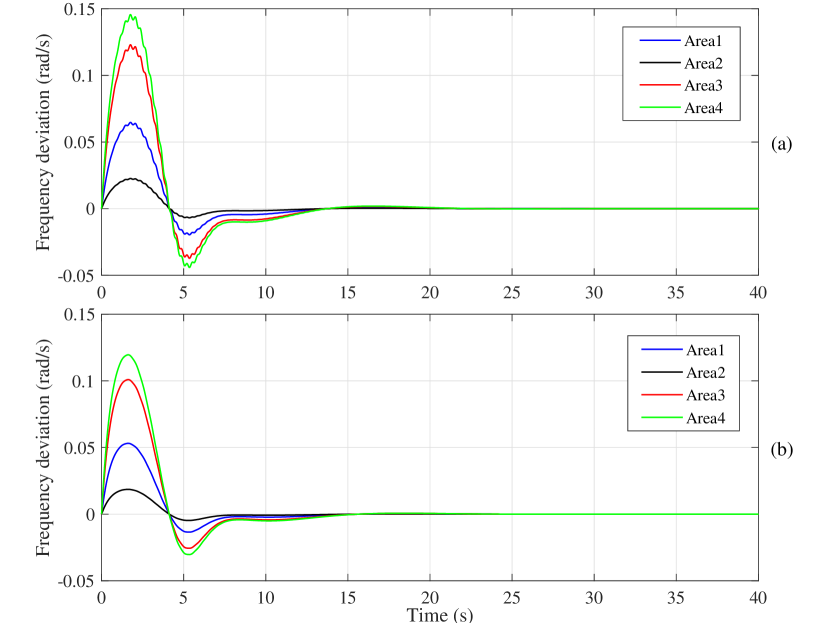
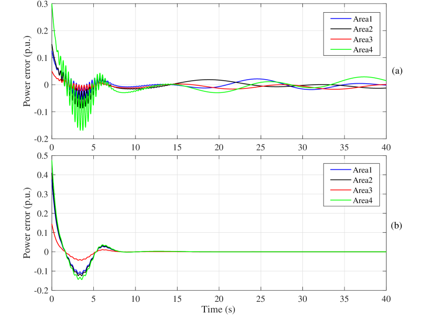
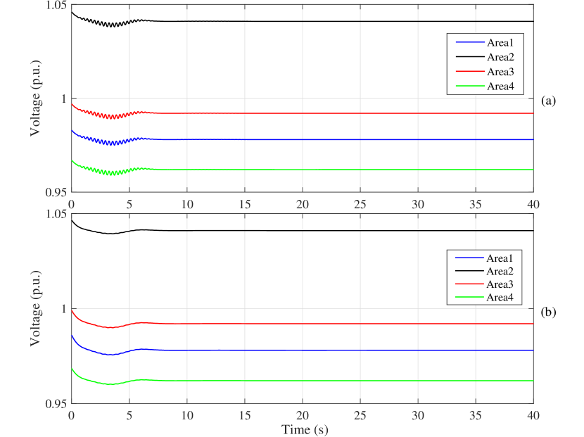
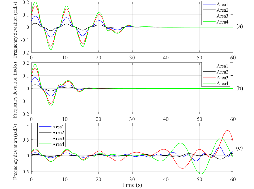
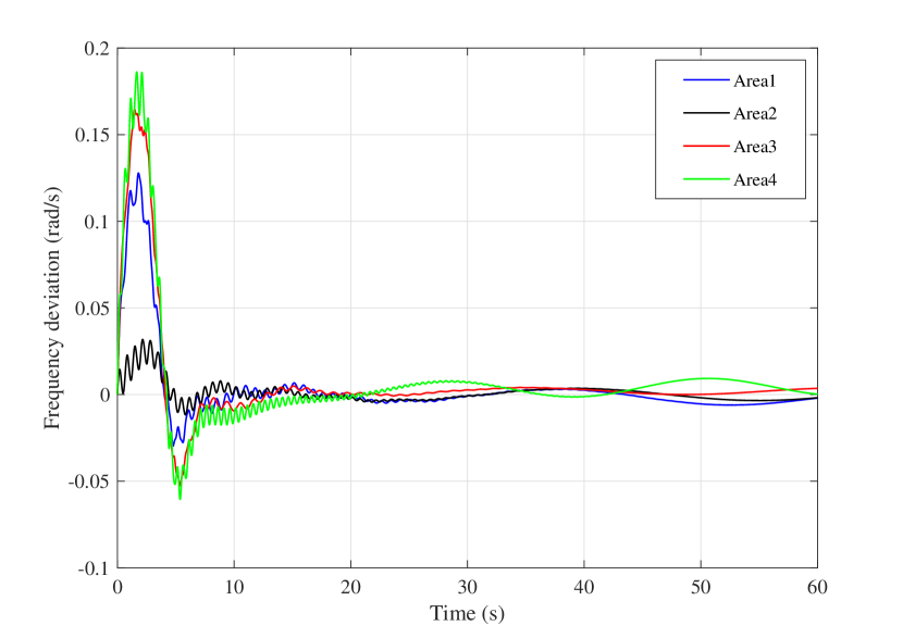
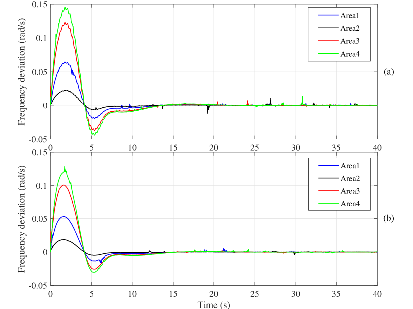
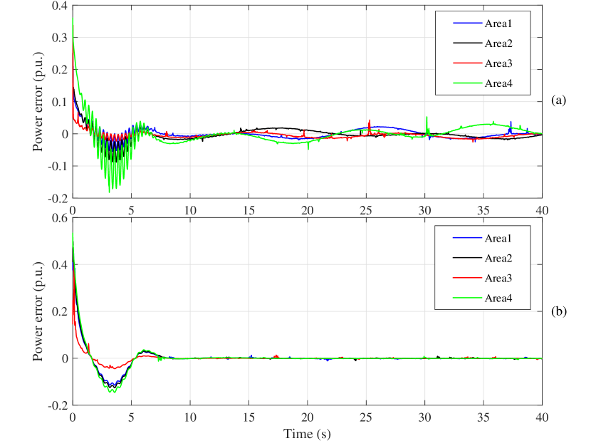
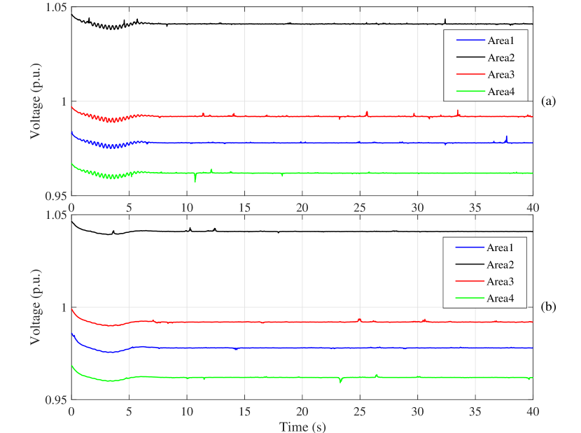
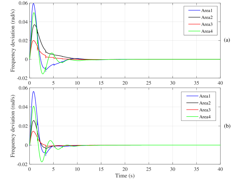
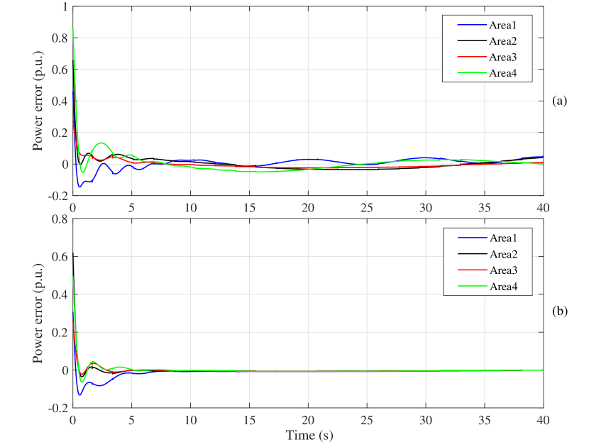
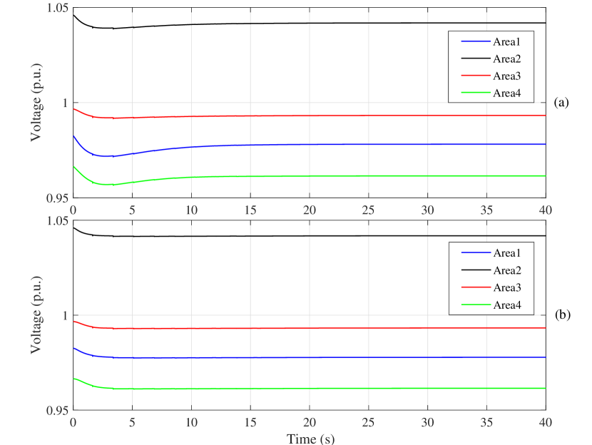
The system is initially at the steady-state with constant uncontrolled power injections. Then, at the initial time instant $t=$ $0\text{\,}\mathrm{s}$, the power generated by the renewable sources and absorbed by the loads is given by (33) and (34), respectively. Fig. 2 shows the frequency deviations when the classical (see Fig. 2a) and approximate (see Fig. 2b) output regulation control approaches are applied, respectively. We can notice that the frequency deviations converge to zero in both cases. Additionally, let $P_{e}:=P_{c}-P_{c}^{\mathrm{opt}}$ denote the error between the actual generated power and its corresponding optimal value given by (11). These errors are shown in Fig. 3 when the classical (see Fig. 3a) and approximate (see Fig. 3b) output regulation control approaches are applied, respectively. Although these errors are bounded in both cases, it is evident that the approximate output regulation control approach achieves Objective 2. Moreover, as discussed in Remark 6, we notice that by choosing $\bar{\epsilon}$ sufficiently small ($\bar{\epsilon}=10^{-7}$), the approximate output regulation control approach achieves in practice OLFC. Indeed, by inspecting the time evolution of the norm of the error defined in (27), it appears that its value becomes smaller than $1\text{\times}{10}^{-3}$ at $t=$ $16\text{\,}\mathrm{s}$ and smaller than $1\text{\times}{10}^{-6}$ at $t=$ $100\text{\,}\mathrm{s}$, implying that Objective 2 is achieved with $\epsilon=$ $1\text{\times}{10}^{-6}$ (the plot is not reported due to space limitation). It is then clear that such an error is in practice definitely negligible when affecting the frequency deviation or power error. Also, we have tested the approximate output regulation control approach in presence of constant power injections and by selecting $\bar{\epsilon}$ equal to zero, achieving OLFC (the plot is not reported due to space limitation). Moreover, we can observe from Fig. 4 that also the voltages are stable. Finally, we can conclude that both the control approaches show good performance and guarantee stability. Additionally, the approximate output regulation control approach achieves in practice OLFC. Consider now the case in which the initial conditions of the frequency deviations are not sufficiently close to zero, i.e., $\omega(0)=\operatorname{col}(0.05,0.02,0.09,$ $0.11)$. We can observe from Figures 5 (a) and (b) that by applying the proposed controllers the frequency deviation at each node converges to zero. On the contrary, we can observe from Figure 5 (c) that by applying a controller based on the output regulation theory and using for the design the linearization of the considered nonlinear system around the desired equilibrium, the frequency deviations do not converge to zero. Finally, we also compare our controller with the one proposed in [20], which is designed to deal with linear exosystem models only. We can clearly observe from Figure 6 that the controller in [20] is not capable to achieve frequency regulation due to the nonlinearity of the exosystem (33).

V-B Scenario 2: Measurement Noise

We consider Scenario 1 adding white noises to the measurement of the generated power $P_{c}$. We can observe from Fig. 7 that both the proposed control approaches regulate the frequency deviations to zero, preserving the stability of the overall network. Also, we can observe from Fig. 8 that the power errors in the approximate output regulation control approach converge to zero (achieving in practice OLFC) and in the classical output regulation control approach remain stable. Furthermore, we can notice from Fig. 9 that the voltages in both control methods are stable as well.

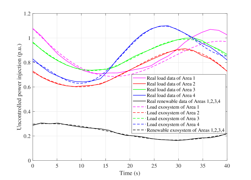
V-C Scenario 3: Real Data for Uncontrolled Power Injections

The system is initially at the steady-state with constant uncontrolled power injections. Then, at the time instant $t=$ $0\text{\,}\mathrm{s}$, we let the uncontrolled power injections vary according to the real values obtained from the dataset [56], (where we use the data of four different areas in the United States, i.e., CAL, CAR, CENT, and FLA for Areas 1, 2, 3, and 4, respectively, on August 29st, 2020), while the controller uses the information of suitable exosystems, which we have tuned in order to let them generate uncontrolled power injection trajectories that approximate well but not exactly the real ones (see Fig. 10). Specifically, we design exosystems that produce the following load: $P_{l}=11.88\sin(0.059t+0.89)+11.19\sin(0.063t+3.96)+0.0375$ for Area 1, $P_{l}=0.814\sin(0.032t+1.27)+0.262\sin(0.121t+3.56)+0.05$ for Area 2, $P_{l}=0.968\sin(0.016t+1.75)+0.211\sin(0.134t+3.28)+0.0375$ for Area 3, $P_{l}=1.129\sin(0.011t+0.65)+0.168\sin(0.209t+2.42)+0.0125$ for Area 4, and the following renewable generation: $P_{w}=0.19\sin(0.007t+1.22)+0.071\sin(0.117t+1.26)+0.05$ for all the areas. Thus, the exosystem (8) can be expressed as

$$\begin{split}\dot{d}^{a}_{yi}&=0\\ \dot{d}^{b}_{yi}&=\left(\begin{array}[]{cccc}0&-\omega^{\alpha}_{yi}&0&0\\ \omega^{\alpha}_{yi}&0&0&0\\ 0&0&0&-\omega^{\beta}_{yi}\\ 0&0&\omega^{\beta}_{yi}&0\end{array}\right)d^{b}_{yi}\\ P_{yi}&=\Gamma_{yi}\operatorname{col}\big{(}d^{a}_{yi},d^{b}_{yi}\big{)},\end{split}$$ (35)

where ${d}^{a}_{yi}:\mathbb{R}_{\geq 0}\rightarrow\mathbb{R}$, $d^{b}_{yi}:\mathbb{R}_{\geq 0}\rightarrow\mathbb{R}^{4}$ are the states of the exosystem, $\omega^{\alpha}_{yi}$, $\omega^{\beta}_{yi}$ are equal to the frequency of the sinusoidal terms in $P_{l}$ and $P_{w}$. Moreover, the elements of the matrix $\Gamma_{yi}$ can be obtained from the amplitude and phase of the sinusoidal terms in $P_{l}$ and $P_{w}$, where $y$ denotes $l$ or $w$ in case of load demand or renewable generation, respectively. Note that, system (35) belongs to the class of exosystems we consider in (9). We can observe from Fig. 11 that, despite the mismatch between the actual uncontrolled power injections and the ones generated by the corresponding exosystems, the frequency deviation at each node converges to zero in both classical and approximate output regulation methods, showing that the controlled system is ISS with respect to such a mismatch. We can also observe from Fig. 12 that also in this scenario the approximate output regulation control approach achieves in practice OLFC. Moreover, Fig. 13 clearly shows that the voltages are stable as well.

VI Conclusion

In this paper, we have used the output regulation theory for the design and analysis of control schemes for nonlinear power networks affected by time-varying renewable energy sources and loads. More precisely, based on the classical output regulation theory we have proposed a controller that provably regulates the frequency deviation to zero even in presence of time-varying uncontrolled power injections. Then, besides merely controlling the frequency deviation, we have proposed a controller that additionally reduces the generation costs. Future research includes the modelling of the uncontrolled power injections as stochastic differential equations and the use of the Ito calculus framework to tackle the problem of OLFC in power networks.

In this Appendix, we present the proofs of Lemma 1, Theorem 2, and Proposition 1.

-A Proof of Lemma 1

Proof:

We use the definition of relative degree given in [43, Definition 2.47]. Then, we have

$$\begin{split}L_{g_{a}}h=&~{}\big{(}\bm{0}_{n\times m}~{}\mathds{I}_{n}~{}\bm{0}_{n\times n}~{}\bm{0}_{n\times n}~{}\bm{0}_{n\times n}~{}\bm{0}_{n\times n(n_{d}+1)}\big{)}g_{a}\\ =&~{}\bm{0}_{n\times n}\\ L_{f_{a}}h=&~{}\big{(}\bm{0}_{n\times m}~{}\mathds{I}_{n}~{}\bm{0}_{n\times n}~{}\bm{0}_{n\times n}~{}\bm{0}_{n\times n}~{}\bm{0}_{n\times n(n_{d}+1)}\big{)}f_{a}\\ =&~{}\tau_{p}^{-1}\Big{(}-\psi\omega+P_{c}+\Gamma d-\mathcal{A}\Upsilon(V)\sin(\theta)\Big{)}\\ L_{g_{a}}L_{f_{a}}h=&~{}\tau_{p}^{-1}\tau_{c}^{-1},\end{split}$$ (36)

implying that the relative degree for each control area is equal to 2. ∎

-B Proof of Theorem 2

Proof:

By virtue of [43, Theorem 3.26], we first compute the following matrix

$$\begin{split}G_{e}(x,d)=\left(\begin{array}[]{c}h(x,d)\\ L_{f_{a}}h(x,d)\\ \end{array}\right),\end{split}$$ (37)

Then, we notice that the solution to $G_{e}(x,d)=\bm{0}_{2n}$ for system (15) can be obtained as follows:

$$\begin{split}\bm{0}_{n}&=\omega^{\ast}\\ \bm{0}_{n}&=P_{c}+\Gamma d-\mathcal{A}\Upsilon(V)\sin(\theta^{\ast}).\end{split}$$ (38)

where $\omega^{\ast}=\bm{0}_{n}$ and $\theta^{\ast}$ denote the solutions to (38). Thus, there exist the partition $x^{a}:=\operatorname{col}(\theta,\omega),x^{b}:=\operatorname{col}(V,P_{c},\delta)$ and a sufficiently smooth function

$$\begin{split}\zeta(x^{b},d):=\left(\begin{array}[]{c}\theta^{\ast}\\ \bm{0}_{n}\end{array}\right),\end{split}$$ (39)

such that $G_{e}(x,d)|_{x^{a}=\zeta(x^{b},d)}=\bm{0}_{2n}$. Recalling that for each $i=1,\dots,n$, the $i$-th output $h_{i}$ of system (15) has relative degree equal to 2 (see Lemma 1), we compute the equivalent control input $u_{e}(x,d)$ by posing the second-time derivate of the output mapping (15c) equal to zero, i.e.,

$$L_{f_{a}}^{2}h(x,d)+L_{g_{a}}L_{f_{a}}h(x,d)u_{e}(x,d)=\bm{0}_{n},$$ (40)

obtaining the following expression:

$$\begin{split}u_{e}(x,d)=&-(\tau_{p}^{-1}\tau_{c}^{-1})^{-1}D_{a}(x,d)\\ =&~{}\tau_{c}\mathcal{A}\Upsilon(V)[\cos(\theta)]\mathcal{A}^{\top}\omega-\tau_{c}\tau_{p}^{-1}\psi^{2}\omega\\ &+\tau_{c}\tau_{p}^{-1}\psi\Big{(}P_{c}+\Gamma d-\mathcal{A}\Upsilon(V)\sin(\theta)\Big{)}\\ &-\tau_{c}\tau_{v}^{-1}\mathcal{A}[\sin(\theta)]\Upsilon(V)|\mathcal{A}|[V]^{-1}\Big{(}\chi_{d}E(\theta)V\\ &-\bar{E}_{f}\Big{)}+P_{c}+\xi^{-1}\omega-\tau_{c}\Gamma S(d).\end{split}$$ (41)

Now, let $u_{e}^{\ast}(x,d):=u_{e}(x,d)|_{x^{a}=\zeta(x^{b},d)}$. By replacing $\omega$ and $\theta$ in (41) with $\omega^{\ast}$ and $\theta^{\ast}$ given in (38), we obtain

$$\begin{split}u_{e}^{\ast}(x,d)=&~{}u_{e}(x,d)|_{x^{a}=\zeta(x^{b},d)}\\ =&-\tau_{c}\tau_{v}^{-1}\mathcal{A}[\sin(\theta)]\Upsilon(V)|\mathcal{A}|[V]^{-1}\Big{(}\chi_{d}E(\theta^{\ast})V\\ &-\bar{E}_{f}\Big{)}+P_{c}-\tau_{c}\Gamma S(d).\end{split}$$ (42)

Then, the zero dynamics of (15) are given by

$$\begin{split}\tau_{v}\dot{V}=&-\chi_{d}E(\theta^{\ast})V+\bar{E}_{f}\\ \tau_{c}\dot{P}_{c}=&-P_{c}+u_{e}^{\ast}(x,d)\\ \tau_{\delta}\dot{\delta}=&-\delta+P_{c}-\xi^{-1}QL^{\mathrm{com}}(Q\delta+R)\\ \dot{d}=&~{}S(d),\end{split}$$ (43)

which can be rewritten as

$$\begin{split}\dot{x}^{b}&=\varrho({x}^{b}(d),d)\\ \dot{d}&=S(d),\end{split}$$ (44)

where $\varrho({x}^{b}(d),d)$ is given by (21). Now, we replace ${x}^{b}$ in (44) with the solution $\bm{x}^{b}(d)$ to (20) and define $\bm{\theta}(d):=\theta^{\ast}(\bm{x}^{b}(d))$. Thus, according to [43, Theorem 3.26], the solution to the regulator equation (19) can be expressed as follows:

$$\begin{split}\bm{x}(d)=&\left(\begin{array}[]{c}\bm{\theta}(d)\\ \bm{0}_{n}\\ \bm{x}^{b}(d)\end{array}\right)\\ \bm{u}(d)=&~{}u_{e}^{\ast}(\bm{x}(d),d),\end{split}$$ (45)

where ${u}^{\ast}_{e}\big{(}\bm{x}(d),d\big{)}$ is given by (24). Hence, following Theorem 1, Problem 1 is solvable. Then, the state feedback controller (23) guarantees that the trajectories of the closed-loop system (4), (7), (9), (23) starting sufficiently close to $(\bar{\theta},\bm{0}_{n},\bar{V},\bar{P}_{c},\bar{\delta},\bar{d})$ are bounded and converge to the set where the frequency deviation is equal to zero, achieving Objective 1. ∎

In the proof of Theorem 2, we have provisionally assumed that the solution to (20) exist. In the following proposition, the condition for the solvability of the regulator equation (19), implying the solvability of (20), is investigated.

Proposition 2

(Existence of solution to the regulator equation (19)). The solution to regulator equation (19) exists if $A_{11}$ has no zero real part eigenvalue and for all $\rho\in\mathbb{R}$

$$\begin{split}\det\big{(}A_{22}-j\rho\mathds{I}_{n}-A_{21}(A_{11}-j\rho\mathds{I}_{n})^{-1}A_{12}\big{)}\neq 0,\end{split}$$ (46)

where

$$\begin{split}A_{11}&=-\frac{\partial\big{(}\tau_{v}^{-1}\chi_{d}E(\theta^{\ast}(x^{b}(d))){V}\big{)}}{\partial V}\Big{|}_{(x,d)=(\bar{x},\bar{d})}\\ A_{12}&=-\frac{\partial\big{(}\tau_{v}^{-1}\chi_{d}E(\theta^{\ast}(x^{b}(d))){V}\big{)}}{\partial P_{c}}\Big{|}_{(x,d)=(\bar{x},\bar{d})}\\ A_{21}&=\tau_{c}^{-1}\frac{\partial u_{e}^{\ast}(x,d)}{\partial V}\Big{|}_{(x,d)=(\bar{x},\bar{d})}\\ A_{22}&=-\tau_{c}^{-1}+\tau_{c}^{-1}\dfrac{\partial u_{e}^{\ast}(x,d)}{\partial P_{c}}\Big{|}_{(x,d)=(\bar{x},\bar{d})}\\ A_{33}&=-\tau_{\delta}^{-1}\big{(}\mathds{I}_{n}+\xi^{-1}QL^{\mathrm{com}}Q\big{)},\end{split}$$ (47)

$\theta^{\ast}(x^{b}(d))$ is the solution to (38), $u_{e}^{\ast}(x,d)$ is given by (42), and $(\bar{x},\bar{d})$ satisfies (13).

Proof:

We have discussed in Remark 4 that the solution to the regulator equation (19) exists if all the eigenvalues of the matrix

$$\begin{split}A&:=\frac{\partial\varrho(x^{b},d)}{\partial x^{b}}\Big{|}_{(x,d)=(\bar{x},\bar{d})}\\ &=\left(\begin{array}[]{ccc}A_{11}&A_{12}&\bm{0}\\ A_{21}&A_{22}&\bm{0}\\ \bm{0}&\tau_{\delta}^{-1}&A_{33}\end{array}\right),\end{split}$$ (48)

have nonzero real part, where $A_{ij},i,j=1,2,3$ are defined in (47). Now, let $\lambda$ denotes the eigenvalues of matrix $A$. Then, by using the Schur complement of the block $A_{33}-\lambda\mathds{I}_{n}$ of the matrix $A-\lambda\mathds{I}_{3n}$, the eigenvalues of $A$ satisfy

$$\begin{split}\det\big{(}A-\lambda\mathds{I}_{3n}\big{)}=&~{}\det\big{(}A_{33}-\lambda\mathds{I}_{n}\big{)}\cdot\\ &~{}\det\underbrace{\left(\begin{array}[]{cc}A_{11}-\lambda\mathds{I}_{n}&A_{12}\\ A_{21}&A_{22}-\lambda\mathds{I}_{n}\end{array}\right)}_{:=\,\tilde{A}}\\ =&~{}\det\big{(}A_{33}-\lambda\mathds{I}_{n}\big{)}\cdot\det\big{(}A_{11}-\lambda\mathds{I}_{n}\big{)}\cdot\\ &\det\Big{(}A_{22}-\lambda\mathds{I}_{n}\\ &-A_{21}(A_{11}-\lambda\mathds{I}_{n})^{-1}A_{12}\Big{)}\\ =&~{}0,\end{split}$$ (49)

where the second equality is obtained by using again the Schur complement of the block $A_{11}-\lambda\mathds{I}_{n}$ of the matrix $\tilde{A}$. We notice that the matrices $\xi$ and $Q$ are positive definite matrices and $L^{\mathrm{com}}$ is a positive semi-definite matrix. Therefore, $A_{33}$ is a negative definite matrix. Also, by virtue of the assumptions in the Proposition statement, $A_{11}$ has no zero real part eigenvalues and (46) holds for all $\rho\in\mathbb{R}$. Then all the eigenvalues of $A$ have nonzero real parts. Consequently, according to [43, Corollary 3.27] the solution to the regulator equation (19) exists. ∎

References

- [1] J. Machowski, J. Bialek, and D. J. Bumby, Power System Dynamics: Stability and Control, 2nd ed. Wiley, 2008.
- [2] A. Wood and B. Wollenberg, Power Generation, Operation, and Control, 2nd ed. Wiley, 1996.
- [3] S. Trip, and C. De Persis, “Distributed optimal Load Frequency Control with non-passive dynamics,” IEEE Transactions on Control of Network Systems, vol. 5, no. 3 pp. 1232-1244, 2018.
- [4] D. Apostolopoulou, P. W. Sauer, and A. D. Domnguez-Garca, “Distributed optimal load frequency control and balancing authority area coordination,” in Proc. of the North American Power Symposium (NAPS), pp. 1-5, 2015.
- [5] D. Cai, E. Mallada, and A. Wierman, “Distributed optimization decomposition for joint economic dispatch and frequency regulation,” IEEE Transactions on Power Systems, vol. 32, no. 6, pp. 4370-4385, 2015.
- [6] S. Trip, M. Cucuzzella, and C. De Persis, A. J. van der Schaft, and A. Ferrara, “Passivity based design of sliding modes for optimal Load Frequency Control,” IEEE Transactions on Control Systems Technology, vol. 27, no. 5, pp. 1893-1906, 2019.
- [7] D. Apostolopoulou, A. D. Domnguez-Garca, and P. W. Sauer, “An assessment of the impact of uncertainty on automatic generation control systems,” IEEE Transactions on Power Systems, pp. 2657-2665, 2016.
- [8] Ibraheem, P. Kumar, and D. P. Kothari, “Recent philosophies of automatic generation control strategies in power systems,” IEEE Transactions on Power Systems, vol. 20, no. 1, pp. 346-357, Feb. 2005.
- [9] S. K. Pandey, S. R. Mohanty, N. Kishor, “A literature survey on load-frequency control for conventional and distribution generation power systems,” Renewable and Sustainable Energy Reviews, vol. 25, pp. 318-334, Sep. 2013.
- [10] F. Dorfler, J. W. Simpson-Porco, and F. Bullo, “Breaking the Hierarchy: Distributed Control and Economic Optimality in Microgrids,” IEEE Transactions on Control of Network Systems, vol. 3, no. 3, pp. 241-253, 2016.
- [11] J. Schiffer and F. Dorfler, “On stability of a distributed averaging PI frequency and active power controlled differential-algebraic power system model,” in Proc. of the 15th European Control Conference (ECC), Aalborg, DK, pp. 1487-1492, 2016.
- [12] N. Rahbari-Asr, U. Ojha, Z. Zhang, and M. Y. Chow, “Incremental welfare consensus algorithm for cooperative distributed generation/demand response in smart grid,” IEEE Transactions on Smart Grid, vol. 5, no. 6, pp. 2836-2845, 2014.
- [13] C. Zhao, E. Mallada, and F. Dorfler, “Distributed frequency control for stability and economic dispatch in power networks,” in Proc. of th 2015 American Control Conference (ACC), pp. 2359-2364, 2015.
- [14] S. Kar and G. Hug, “Distributed robust economic dispatch in power systems: A consensus innovations approach,” in Pro. of the 2012 IEEE Power and Energy Society General Meeting, pp. 1-8, 2012.
- [15] S. Yang, S. Tan, and J. X. Xu, “Consensus based approach for economic dispatch problem in a smart grid,” IEEE Transactions on Power Systems, vol. 28, no. 4, pp. 4416-4426, 2013.
- [16] N. Monshizadeh, C. De Persis, A. J. van der Schaft, and J. Scherpen, “A novel reduced model for electrical networks with constant power loads,” IEEE Transactions on Automatic Control, vol. 63,. no. 5, 1288-1299, 2018.
- [17] T. Yang, D. Wu, Y. Sun, and J. Lian, “Minimum-time consensus based approach for power system applications,” IEEE Transactions on Industrial Electronics, vol. 63, no. 2, pp. 1318-1328, 2016.
- [18] G. Binetti, A. Davoudi, F. L. Lewis, D. Naso, and B. Turchiano, “Distributed consensus-based economic dispatch with transmission losses,” IEEE Transactions on Power Systems, vol. 29, no. 4, pp. 1711-1720, 2014.
- [19] Z. Zhang and M. Y. Chow, “Convergence analysis of the incremental cost consensus algorithm under different communication network topologies in a smart grid,” IEEE Transactions on Power Systems, vol. 27, no. 4, pp. 1761-1768, 2012.
- [20] S. Trip, M. Burger, and C. De Persis, “An internal model approach to (optimal) frequency regulation in power grids with time-varying voltages,” Automatica, vol. 64, pp. 240-253, 2016.
- [21] M. Burger, C. De Persis, and S. Trip, “An internal model approach to (optimal) frequency regulation in power grids” in Proc. of the 21th International Symposium on Mathematical Theory of Networks and Systems (MTNS), Groningen, the Netherlands, 2014, pp. 577-583.
- [22] X. Zhang and A. Papachristodoulou,“A real-time control framework for smart power networks: Design methodology and stability,” Automatica, vol. 58, pp. 43-50, 2015.
- [23] N. Li, C. Zhao, and L. Chen, “Connecting automatic generation control and economic dispatch from an optimization view,” IEEE Transactions on Control of Network Systems, vol. 3, no. 3, pp. 254-264, 2016.
- [24] T. Stegink, C. De Persis, and A. J. van der Schaft, “A unifying energy-based approach to stability of power grids with market dynamics,” IEEE Transactions on Automatic Control, vol. 62, no. 6, pp. 2612-2622, 2017.
- [25] L. Chen and S. You, “Reverse and forward engineering of frequency control in power networks,” IEEE Transactions on Automatic Control, vol. 62, no. 2, pp. 4631-4638, 2017.
- [26] A. Kasis, E. Devane, C. Spanias, and I. Lestas, “Primary frequency regulation with load-side participation part I: stability and optimality,” IEEE Transactions on Power Systems, vol. 32, no. 5, pp. 3505-3518, 2017.
- [27] P. Yi, Y. Hong, and F. Liu, “Initialization-free distributed algorithms for optimal resource allocation with feasibility constraints and application to economic dispatch of power systems,” Automatica, vol. 74, pp. 259-269, 2016.
- [28] A. Cherukuri and J. Cortes, “Initialization-free distributed coordination for economic dispatch under varying loads and generator commitment,” Automatica, vol. 74, pp. 183-193, 2016.
- [29] P. Yi, Y. Hong, and F. Liu, “Distributed gradient algorithm for constrained optimization with application to load sharing in power systems,” Systems & Control Letters, vol. 83, pp. 45-52, 2015.
- [30] R. Mudumbai, S. Dasgupta, and B. B. Cho, “Distributed control for optimal economic dispatch of a network of heterogeneous power generators,” IEEE Transactions on Power Systems,vol. 27, no. 4, pp. 1750-1760, 2012.
- [31] A. Jokic, M. Lazar, and P. van den Bosch, “Real-time control of power systems using nodal prices,” International Journal of Electrical Power & Energy Systems, vol. 31, no. 9, pp. 522-530, 2009.
- [32] Z. Miao and L. Fan, “Achieving economic operation and secondary frequency regulation simultaneously through local feedback control,” IEEE Transactions on Power Systems, vol. 32, no. 99, pp. 1-9, 2017.
- [33] J. W. Simpson-Porco, F. Dorfler, and F. Bullo, “Synchronization and power sharing for droop-controlled inverters in islanded microgrids,” Automatica, vol. 49, no. 9, pp. 2603-2611, 2013.
- [34] J. M. Guerrero, J. C. Vasquez, J. Matas, L. G. de Vicuna, and M. Castilla,“Hierarchical control of droop-controlled ac and dc microgrids, a general approach toward standardization,” IEEE Transactions on Industrial Electronics, vol. 58, no. 1, pp. 158-172, 2011.
- [35] J. Schiffer, R. Ortega, A. Astolfi, J. Raisch, and T. Sezi,“Synchronization of droop-controlled microgrids with distributed rotational and electronic generation,” Proc. of the IEEE 52nd Conference on Decision and Control (CDC), pp. 2334-2339, 2013.
- [36] S. Trip, M. Cucuzzella, C. De Persis, A. Ferrara, and J. M. A. Scherpen, “Robust load frequency control of nonlinear power networks,” International Journal of Control, vol. 93, no. 2, 2020.
- [37] N. Li, C. Zhao, and. Chen, “Connecting automatic generation control and economic dispatch from an optimization view,” IEEE Transactions on Control of Network Systems, Vol. 3, no. 3, pp. 254-264, 2016.
- [38] C. Zhao and S. Low, “Decentralized primary frequency control in power networks,” 53rd IEEE Conference on Decision and Control, 2014.
- [39] F. Dorfler, and S. Grammatico “Gather-and-broadcast frequency control in power systems,” Automatica, vol. 79, pp. 296-305, 2017.
- [40] T. Stegink, A. Cherukuri, C. De Persis, A. J. van der Schaft, J. Cortes, “Frequency-driven market mechanisms for optimal dispatch in power networks,” arXiv preprint arXiv:1801.00137 [math.OC], 2017.
- [41] G. Rinaldi, P. P. Menon, C. Edwards, and A. Ferrara, “Distributed Super-Twisting Sliding Mode Observers for Fault Reconstruction and Mitigation in Power Networks,” 2018 IEEE Conference on Decision and Control (CDC), Miami Beach, Florida, USA, 2018.
- [42] G. Rinaldi, P. P. Menon, C. Edwards, and A. Ferrara, “Higher Order Sliding Mode Observers in Power Grids With Traditional and Renewable Sources,” IEEE Control Systems Letters, vol. 4, no. 1, pp. 223-228, 2020.
- [43] J. Huang, Nonlinear Output Regulation Theory and Applications, Siam, 2004.
- [44] A. Isidori, Nonlinear Control Systems, Springer, 1995.
- [45] H. Verdejo, A. Awerkin, E. Saavedra, W. Kliemann, L. Vargas, “Stochastic modeling to represent wind power generation and demand in electric power system based on real data,” Applied Energy, vol. 173, pp. 283-295, 2016.
- [46] Z. Wang, H. He, and Y. Sun, “Robust Frequency Control of Power Systems Under Time-varying Loads,” North American Power Symposium (NAPS), Wichita, KS, USA, 2019.
- [47] A. Arif, Z. Wang, J. Wang, B. Mather, H. Bashualdo, and D. Zhao, “Load Modeling-A Review,” IEEE Transactions on Smart Grid, vol. 9, no. 6, pp. 5986-5999, 2018.
- [48] B. K. Choi and H. D. Chiang, “Multiple Solutions and Plateau Phenomenon in Measurement-Based Load Model Development: Issues and Suggestions,” IEEE Transactions on Power Systems, vol. 24, no. 2, pp. 824-831, 2009.
- [49] Y. Ge, A. J. Flueck, D. K. Kim, J. B. Ahn, J. D. Lee, and D. Y. Kwon, “An Event-Oriented Method for Online Load Modeling Based on Synchrophasor Data,” IEEE Transactions on Smart Grid, vol. 6, no. 4, pp. 2060-2068, 2015.
- [50] D. J. Hill, “Nonlinear dynamic load models with recovery for voltage stability studies,” IEEE Transactions on Power Systems, vol. 8, no. 1, pp. 166-176, Feb., 1993.
- [51] A. Saberi , A. A. Stoorvogel , P. Sannuti, and G. Shi “On optimal output regulation for linear systems,” International Journal of Control, vol. 76, no. 4 pp. 319-333, 2003.
- [52] B. Rehak, and S. Celikovsk, “Numerical method for the solution of the regulator equation with application to nonlinear tracking,” Automatica, vol. 44, no. 5, pp. 1358-1365, 2008.
- [53] L. S. P. Lawrence, J. W. Simpson-Porco, and E. Mallada, “Linear-Convex Optimal Steady-State Control,” arXiv preprint arXiv:1810.12892 [math.OC], 2019.
- [54] M. Olsson, M. Perninge, and L. Soder, “Modeling real-time balancing power demands in wind power systems using stochastic differential equations,” Applied Energy, vol. 80, no. 8, pp. 966-974, 2010.
- [55] S. Nabavi and A. Chakrabortty, “Topology identification for dynamic equivalent models of large power system networks,” in Proc. of the 2013 American Control Conference (ACC), pp. 1138-1143, 2013.
-
[56]
Hourly Electric Grid Monitor, https://www.eia.gov/beta/electricity/
gridmonitor/dashboard/electric-overview/US48/US48.