Constructing Taxonomies from Pretrained Language Models

Abstract

We present a method for constructing taxonomic trees (e.g., WordNet) using pretrained language models. Our approach is composed of two modules, one that predicts parenthood relations and another that reconciles those predictions into trees. The parenthood prediction module produces likelihood scores for each potential parent-child pair, creating a graph of parent-child relation scores. The tree reconciliation module treats the task as a graph optimization problem and outputs the maximum spanning tree of this graph. We train our model on subtrees sampled from WordNet, and test on non-overlapping WordNet subtrees. We show that incorporating web-retrieved glosses can further improve performance. On the task of constructing subtrees of English WordNet, the model achieves 66.7 ancestor $F_{1}$, a 20.0% relative increase over the previous best published result on this task. In addition, we convert the original English dataset into nine other languages using Open Multilingual WordNet and extend our results across these languages.

1 Introduction

A variety of NLP tasks use taxonomic information, including question answering (Miller, 1998) and information retrieval (Yang and Wu, 2012). Taxonomies are also used as a resource for building knowledge and systematicity into neural models (Peters et al., 2019; Geiger et al., 2020; Talmor et al., 2020). NLP systems often retrieve taxonomic information from lexical databases such as WordNet (Miller, 1998), which consists of taxonomies that contain semantic relations across many domains. While manually curated taxonomies provide useful information, they are incomplete and expensive to maintain (Hovy et al., 2009).

Traditionally, methods for automatic taxonomy construction have relied on statistics of web-scale corpora. These models generally apply lexico-syntactic patterns (Hearst, 1992) to large corpora, and use corpus statistics to construct taxonomic trees (e.g., Snow et al., 2005; Kozareva and Hovy, 2010; Bansal et al., 2014; Mao et al., 2018; Shang et al., 2020).

Figure 1: An example subtree from the WordNet hierarchy.

In this work, we propose an approach that constructs taxonomic trees using pretrained language models (CTP). Our results show that direct access to corpus statistics at test time is not necessary. Indeed, the re-representation latent in large-scale models of such corpora can be beneficial in constructing taxonomies. We focus on the task proposed by Bansal et al. (2014), where the task is to organize a set of input terms into a taxonomic tree. We convert this dataset into nine other languages using synset alignments collected in Open Multilingual Wordnet and evaluate our approach in these languages.

CTP first finetunes pretrained language models to predict the likelihood of pairwise parent-child relations, producing a graph of parenthood scores. Then it reconciles these predictions with a maximum spanning tree algorithm, creating a tree-structured taxonomy. We further test CTP in a setting where models have access to web-retrieved glosses. We reorder the glosses and finetune the model on the reordered glosses in the parenthood prediction module.

We compare model performance on subtrees across semantic categories and subtree depth, provide examples of taxonomic ambiguities, describe conditions for which retrieved glosses produce greater increases in tree construction $F_{1}$ score, and evaluate generalization to large taxonomic trees (Bordea et al., 2016a). These analyses suggest specific avenues of future improvements to automatic taxonomy construction.

Even without glosses, CTP achieves a 7.9 point absolute improvement in $F_{1}$ score on the task of constructing WordNet  subtrees, compared to previous work. When given access to the glosses, CTP obtains an additional 3.2 point absolute improvement in $F_{1}$ score. Overall, the best model achieves a 11.1 point absolute increase (a 20.0% relative increase) in $F_{1}$ score over the previous best published results on this task.

Our paper is structured as follows. In Section 2 we describe CTP, our approach for taxonomy construction. In Section 3 we describe the experimental setup, and in Section 4 we present the results for various languages, pretrained models, and glosses. In Section 5 we analyze our approach and suggest specific avenues for future improvement. We discuss related work and conclude in Sections 6 and 7.

2 Constructing Taxonomies from Pretrained Models

2.1 Taxonomy Construction

We define taxonomy construction as the task of creating a tree-structured hierarchy $T=(V,E)$, where $V$ is a set of terms and $E$ is a set of directed edges representing hypernym relations. In this task, the model receives a set of terms $V$, where each term can be a single word or a short phrase, and it must construct the tree $T$ given these terms. CTP performs taxonomy construction in two steps: parenthood prediction (Section 2.2) followed by graph reconciliation (Section 2.3).

We provide a schematic description of CTP in Figure 2 and provide details in the remainder of this section.

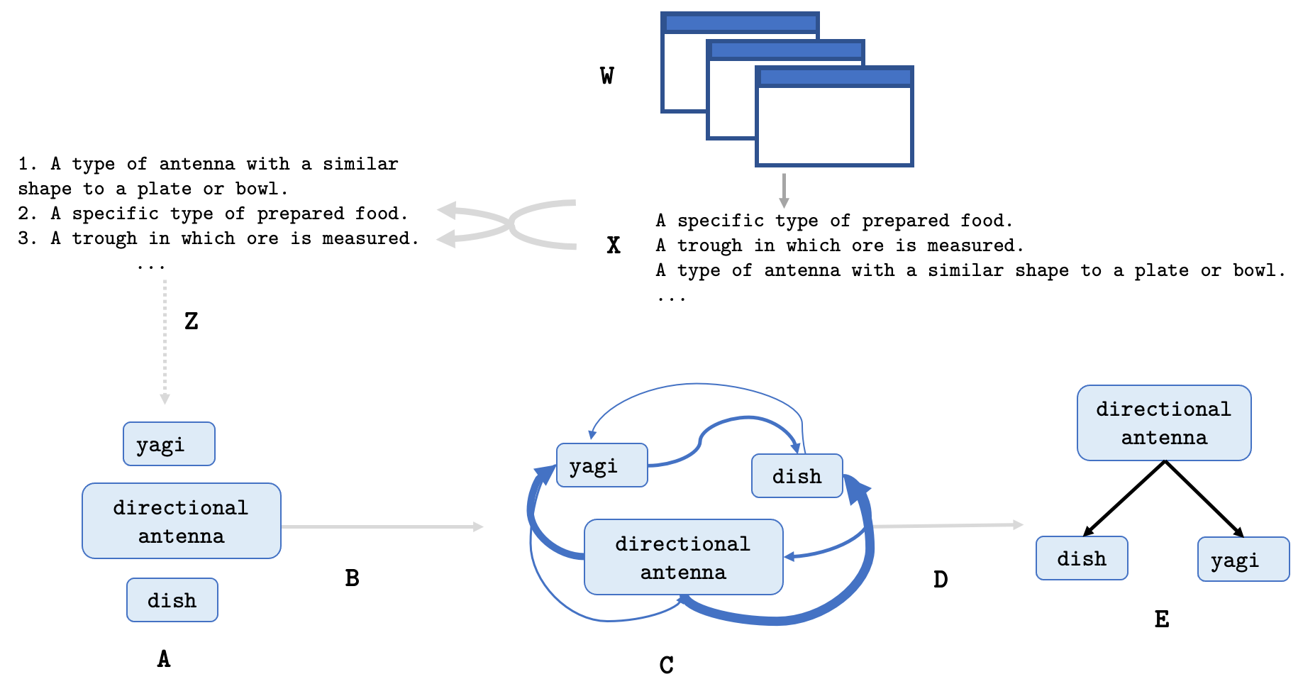
Figure 2: A schematic depiction of CTP. We start with a set of terms (A). We fine-tune a pretrained language model to predict pairwise parenthood relations between pairs of terms (B), creating a graph of parenthood predictions (C) (Section 2.2). We then reconcile the edges of this graph into a taxonomic tree (E) (Section 2.3). Optionally, we provide the model ranked web-retrieved glosses (Section 2.4). We re-order the glosses based on relevance to the current subtree (Z).

2.2 Parenthood Prediction

We use pretrained models (e.g., BERT) to predict the edge indicators $\mathbb{I}[parent(v_{i},v_{j})]$, which denote whether $v_{i}$ is a parent of $v_{j}$, for all pairs $(v_{i},v_{j})$ in the set of terms $V=\{v_{1},...,v_{n}\}$ for each subtree $T$.

To generate training data from a tree $T$ with $n$ nodes, we create a positive training example for each of the $n-1$ parenthood edges and a negative training example for each of the $\frac{n(n-1)}{2}-(n-1)$ pairs of nodes that are not connected by a parenthood edge.

We construct an input for each example using the template $v_{i}$ is a $v_{j}$, e.g., “A dog is a mammal." Different templates (e.g., [TERM_A] is an example of [TERM_B] or [TERM_A] is a type of [TERM_B]) did not substantially affect model performance in initial experiments, so we use a single template. The inputs and outputs are modeled in the standard format (Devlin et al., 2019).

We fine-tune pretrained models to predict $\mathbb{I}[parent(v_{i},v_{j})]$, which indicates whether $v_{i}$ is the parent of $v_{j}$, for each pair of terms using a sentence-level classification task on the input sequence.

2.3 Tree Reconciliation

We then reconcile the parenthood graph into a valid tree-structured taxonomy. We apply the Chu-Liu-Edmonds algorithm to the graph of pairwise parenthood predictions. This algorithm finds the maximum weight spanning arborescence of a directed graph. It is the analog of MST for directed graphs, and finds the highest scoring arborescence in $O(n^{2})$ time (Chu, 1965).

2.4 Web-Retrieved Glosses

We perform experiments in two settings: with and without web-retrieved glosses. In the setting without glosses, the model performs taxonomy construction using only the set of terms $V$. In the setting with glosses, the model is provided with glosses retrieved from the web. For settings in which the model receives glosses, we retrieve a list of glosses $d_{v}^{1},...,d_{v}^{n}$ for each term $v\in V$.

Many of the terms in our dataset are polysemous, and the glosses contain multiple senses of the word. For example, the term dish appears in the subtree we show in Figure 1. The glosses for dish include (1) (telecommunications) A type of antenna with a similar shape to a plate or bowl, (2) (metonymically) A specific type of prepared food, and (3) (mining) A trough in which ore is measured.

We reorder the glosses based on their relevance to the current subtree. We define relevance of a given context $d_{v}^{i}$ to subtree $T$ as the cosine similarity between the average of the GloVe embeddings (Pennington et al., 2014) of the words in $d_{v}^{i}$ (with stopwords removed), to the average of the GloVe embeddings of all terms $v_{1},...,v_{n}$ in the subtree. This produces a reordered list of glosses $d_{v}^{(1)},...,d_{v}^{(n)}$.

We then use the input sequence containing the reordered glosses “[CLS] $v_{i}\>d_{v_{i}}^{(1)},...,d_{v_{i}}^{(n)}$. [SEP] $v_{j}\>d_{v_{j}}^{(1)},...,d_{v_{j}}^{(n)}$” to fine-tune the pretrained models on pairs of terms $(v_{i},v_{j})$.

3 Experiments

In this section we describe the details of our datasets (Section 3.1), and describe our evaluation metrics (Section 3.2). We ran our experiments on a cluster with 10 Quadro RTX 6000 GPUs. Each training runs finishes within one day on a single GPU.

3.1 Datasets

We evaluate CTP using the dataset of medium-sized WordNet subtrees created by Bansal et al. (2014). This dataset consists of bottomed-out full subtrees of height 3 (this corresponds to trees containing 4 nodes in the longest path from the root to any leaf) that contain between 10 and 50 terms. This dataset comprises 761 English trees, with 533/114/114 train/dev/test trees respectively.

3.1.1 Multilingual WordNet

WordNet was originally constructed in English, and has since been extended to many other languages such as Finnish (Magnini et al., 1994), Italian (Lindén and Niemi, 2014), and Chinese (Wang and Bond, 2013). Researchers have provided alignments from synsets in English WordNet to terms in other languages, using a mix of automatic and manual methods (e.g., Magnini et al., 1994; Lindén and Niemi, 2014). These multilingual wordnets are collected in the Open Multilingual WordNet project (Bond and Paik, 2012). The coverage of synset alignments varies widely. For instance, the alignment of Albanet (Albanian) to English WordNet  covers 3.6% of the synsets in the Bansal et al. (2014) dataset, while the FinnWordNet (Finnish) alignment covers 99.6% of the synsets in the dataset.

We convert the original English dataset to nine other languages using the synset alignments. (We create datasets for Catalan (Agirre et al., 2011), Chinese (Wang and Bond, 2013), Finnish (Lindén and Niemi, 2014), French (Sagot, 2008), Italian (Magnini et al., 1994), Dutch (Postma et al., 2016), Polish (Piasecki et al., 2009), Portuguese (de Paiva and Rademaker, 2012), and Spanish (Agirre et al., 2011)).

Since these wordnets do not include alignments to all of the synsets in the English dataset, we convert the English dataset to each target language using alignments specified in WordNet as follows. We first exclude all subtrees whose roots are not included in the alignment between the WordNet of the target language and English WordNet. For each remaining subtree, we remove any node that is not included in the alignment. Then we remove all remaining nodes that are no longer connected to the root of the corresponding subtrees. We describe the resulting dataset statistics in Table 8 in the Appendix.

3.2 Evaluation Metrics

As with previous work (Bansal et al., 2014; Mao et al., 2018), we report the ancestor $F_{1}$ score $\frac{2PR}{P+R}$, where

$$P =\frac{|\mbox{{is\_a}}_{\mbox{{predicted}}}\cap\mbox{{is\_a}}_{\mbox{{gold}}}|}{|\mbox{{is\_a}}_{\mbox{{predicted}}}|}$$

$$R =\frac{|\mbox{{is\_a}}_{\mbox{{predicted}}}\cap\mbox{{is\_a}}_{\mbox{{gold}}}|}{|\mbox{{is\_a}}_{\mbox{{gold}}}|}$$

$\mbox{{is\_a}}_{\mbox{{predicted}}}$ and $\mbox{{is\_a}}_{\mbox{{gold}}}$ denote the set of predicted and gold ancestor relations, respectively. We report the mean precision ($P$), recall ($R$), and $F_{1}$ score, averaged across the subtrees in the test set.

3.3 Models

In our experiments, we use pretrained models from the Huggingface library (Wolf et al., 2019). For the English dataset we experiment with BERT, BERT-Large, and RoBERTa-Large in the parenthood prediction module. We experiment with multilingual BERT and language-specific pretrained models (detailed in Section Language-Specific Pretrained Models in the Appendix). We finetuned each model using three learning rates {1e-5, 1e-6, 1e-7}. For each model, we ran three trials using the learning rate that achieved the highest dev $F_{1}$ score. In Section 4, we report the average scores over three trials. We include full results in Tables 13 and 15 in the Appendix. The code and datasets are available at https://github.com/cchen23/ctp.

4 Results

4.1 Main Results

Our approach, CTP, outperforms existing state-of-the-art models on the WordNet  subtree construction task. In Table 1 we provide a comparison of our results to previous work. Even without retrieved glosses, CTP with RoBERTa-Large in the parenthood prediction module achieves higher $F_{1}$ than previously published work. CTP achieves additional improvements when provided with the web-retrieved glosses described in Section 2.4.

We compare different pretrained models for the parenthood prediction module, and provide these comparisons in Section 4.3.

	P	R	F1
Bansal et al. (2014)	48.0	55.2	51.4
Mao et al. (2018)	52.9	58.6	55.6
CTP (no glosses)	67.3	62.0	63.5
CTP (web glosses)	69.3	66.2	66.7

Table 1: English Results, Comparison to Previous Work. Our approach outperforms previous approaches on reconstructing WordNet subtrees, even when the model is not given web-retrieved glosses.

4.2 Web-Retrieved Glosses

In Table 2 we show the improvement in taxonomy construction with two types of glosses – glosses retrieved from the web (as described in Section 2.4), and those obtained directly from WordNet. We consider using the glosses from WordNet  as an oracle setting since these glosses are directly generated from the gold taxonomies. Thus, we focus on the web-retrieved glosses as the main setting. Models produce additional improvements when given WordNet  glosses. These improvements suggest that reducing the noise from web-retrieved glosses could improve automated taxonomy construction.

	P	R	F1
CTP	67.3	62.0	63.5
+ web glosses	69.3	66.2	66.7
+ oracle glosses	84.0	83.8	83.2

Table 2: English Results, Gloss Comparison on Test Set. Adding web glosses improves performance over only using input terms. Models achieve additional improvements in subtree reconstruction when given oracle glosses from WordNet, showing possibilities for improvement in retrieving web glosses.

4.3 Comparison of Pretrained Models

For both settings (with and without web-retrieved glosses), CTP attains the highest $F_{1}$ score when RoBERTa-Large is used in the parenthood prediction step. As we show in Table 3, the average $F_{1}$ score improves with both increased model size and with switching from BERT to RoBERTa.

	P	R	F1
CTP (BERT-Base)	57.9	51.8	53.4
CTP (BERT-Large)	65.5	59.8	61.4
CTP (RoBERTa-Large)	67.3	62.0	63.5

Table 3: English Results, Comparison of Pretrained Models on Test Set. Larger models perform better and RoBERTa outperforms BERT.

4.4 Aligned Wordnets

We extend our results to the nine non-English alignments to the Bansal et al. (2014) dataset that we created. In Table 4 we compare our best model in each language to a random baseline. We detail the random baseline in Section Random Baseline for Multilingual WordNet Datasets in the Appendix and provide results from all tested models in Section 17 in the Appendix.

	Model	P	R	F1
ca	Random Baseline	20.0	31.3	23.6
	CTP (mBERT)	38.7	39.7	38.0
zh	Random Baseline	25.8	35.9	29.0
	CTP (Chinese BERT)	62.2	57.3	58.7
en	Random Baseline	8.9	22.2	12.4
	CTP (RoBERTa-Large)	67.3	62.0	63.5
fi	Random Baseline	10.1	22.5	13.5
	CTP (FinBERT)	47.9	42.6	43.8
fr	Random Baseline	22.1	34.4	25.9
	CTP (French BERT)	51.3	49.1	49.1
it	Random Baseline	28.9	39.4	32.3
	CTP (Italian BERT)	48.3	45.5	46.1
nl	Random Baseline	26.8	38.4	30.6
	CTP (BERTje)	44.6	44.8	43.7
pl	Random Baseline	23.4	33.6	26.8
	CTP (Polbert)	51.9	49.7	49.5
pt	Random Baseline	26.1	37.6	29.8
	CTP (BERTimbau)	59.3	57.1	56.9
es	Random Baseline	27.0	37.2	30.5
	CTP (BETO)	53.1	51.7	51.7

Table 4: Multilingual WordNet Test Results. We extend our model to datasets in nine other languages, and evaluate our approach on these datasets. We use ISO 639-1 acronyms to indicate languages.

CTP’s $F_{1}$ score non-English languages is substantially worse than its $F_{1}$ score on English trees. Lower $F_{1}$ scores in non-English languages are likely due to multiple factors. First, English pretrained language models generally perform better than models in other languages because of the additional resources devoted to the development of English models. (See e.g., Bender, 2011; Mielke, 2016; Joshi et al., 2020). Second, Open Multilingual Wordnet aligns wordnets to English WordNet, but the subtrees contained in English WordNet might not be the natural taxonomy in other languages. However, we note that scores across languages are not directly comparable as dataset size and coverage vary across languages (as we show in Table 8).

These results highlight the importance of evaluating on non-English languages, and the difference in available lexical resources between languages. Furthermore, they provide strong baselines for future work in constructing wordnets in different languages.

5 Analysis

In this section we analyze the models both quantitatively and qualitatively. Unless stated otherwise, we analyze our model on the dev set and use RoBERTa-Large in the parenthood prediction step.

5.1 Models Predict Flatter Trees

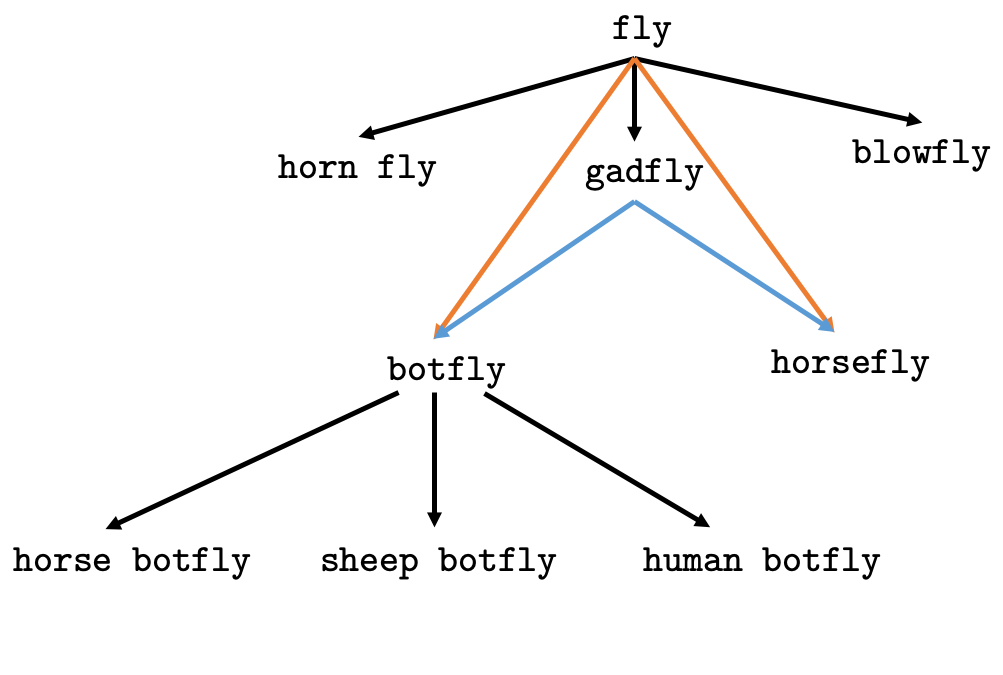
Figure 3: A fragment of a subtree from the WordNet  hierarchy. Orange indicates incorrectly predicted edges and blue indicates missed edges.

In many error cases, CTP predicts a tree with edges that connect terms to their non-parent ancestors, skipping the direct parents. We show an example of this error in Figure 3. In this fragment (taken from one of the subtrees in the dev set), the model predicts a tree in which botfly and horsefly are direct children of fly, bypassing the correct parent gadfly. On the dev set, 38.8% of incorrect parenthood edges were cases of this type of error.

Missing edges result in predicted trees that are generally flatter than the gold tree. While all the gold trees have a height of 3 (4 nodes in the longest path from the root to any leaf), the predicted dev trees have a mean height of 2.61. Our approach scores the edges independently, without considering the structure of the tree beyond local parenthood edges. One potential way to address the bias towards flat trees is to also model the global structure of the tree (e.g., ancestor and sibling relations).

5.2 Model Struggle Near Leaf Nodes

	$d=1$	$d=2$	$d=3$
$l=1$	81.2	52.3	39.7
$l=2$		74.4	48.9
$l=3$			66.0

Table 5: Ancestor Edge Recall, Categorized by Descendant Node Depth $d$ and Parent Edge Length $l$. Ancestor edge prediction recall decreases with deeper descendant nodes and closer ancestor-descendant relations.

CTP generally makes more errors in predicting edges involving nodes that are farther from the root of each subtree. In Table 5 we show the recall of ancestor edges, categorized by the number of parent edges $d$ between the subtree root and the descendant of each edge, and the number of parent edges $l$ between the ancestor and descendant of each edge. The model has lower recall for edges involving descendants that are farther from the root (higher $d$). In permutation tests of the correlation between edge recall and $d$ conditioned on $l$, 0 out of 100,000 permutations yielded a correlation at least as extreme as the observed correlation.

5.3 Subtrees Higher Up in WordNet  are Harder, and Physical Entities are Easier than Abstractions

Subtree performance also corresponds to the depth of the subtree in the entire WordNet  hierarchy. The $F_{1}$ score is positively correlated with the depth of the subtree in the full WordNet hierarchy, with a correlation of 0.27 (significant at p=0.004 using a permutation test with 100,000 permutations).

The subtrees included in this task span many different domains, and can be broadly categorized into subtrees representing concrete entities (such as telephone) and those representing abstractions (such as sympathy). WordNet  provides this categorization using the top-level synsets physical_entity.n.01 and abstraction.n.06. These categories are direct children of the root of the full WordNet  hierarchy (entity.n.01), and split almost all WordNet terms into two subsets. The model produces a mean $F_{1}$ score of 60.5 on subtrees in the abstraction subsection of WordNet, and a mean $F_{1}$ score of 68.9 on subtrees in the physical_entity subsection. A one-sided Mann-Whitney rank test shows that the model performs systematically worse on abstraction subtrees (compared to physical entity subtrees) (p=0.01).

5.4 Pretraining Corpus Covers Most Terms

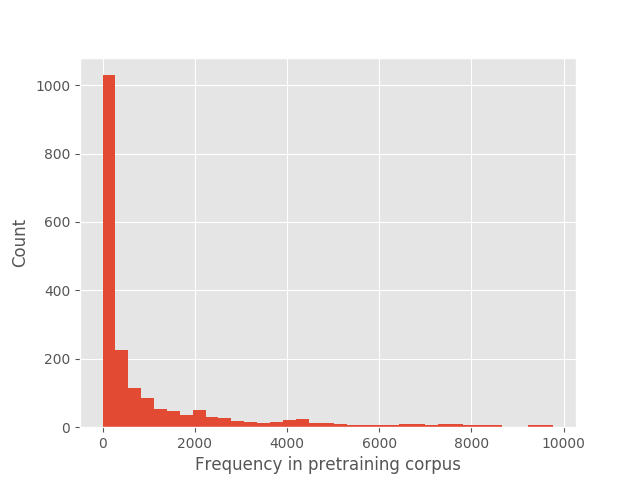
Figure 4: Frequency of terms in the WordNet dataset in the pretraining corpus. Over 97% of terms in the Bansal et al. (2014) dataset occur at least once in the pretraining corpus. Over 80% of terms occur less than 50k times.

With models pretrained on large web corpora, the distinction between the settings with and without access to the web at test time is less clear, since large pretrained models can be viewed as a compressed version of the web. To quantify the extent the evaluation setting measures model capability to generalize to taxonomies consisting of unseen words, we count the number of times each term in the WordNet  dataset occurs in the pretraining corpus. We note that the WordNet glosses do not directly appear in the pretraining corpus. In Figure 4 we show the distribution of the frequency with which the terms in the Bansal et al. (2014) dataset occur in the BERT pretraining corpus. We find that over 97% of the terms occur at least once in the pretraining corpus. However, the majority of the terms are not very common words, with over 80% of terms occurring less than 50k times. While this shows that the current setting does not measure model ability to generalize to completely unseen terms, we find that the model does not perform substantially worse on edges that contain terms that do not appear in the pretraining corpus. Furthermore, the model is able do well on rare terms. Future work can investigate model ability to construct taxonomies from terms that are not covered in pretraining corpora.

5.5 WordNet Contains Ambiguous Subtrees

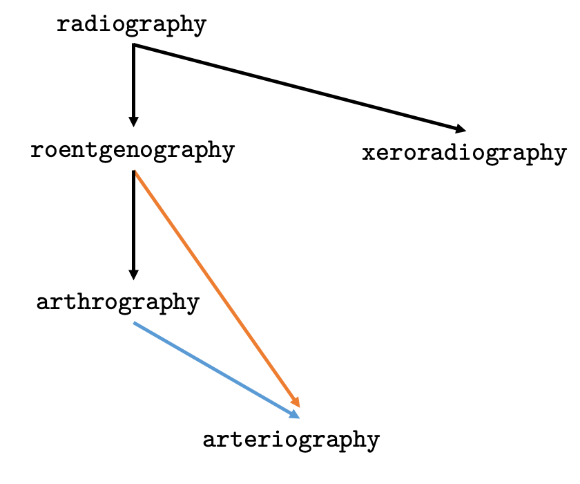
Figure 5: A fragment of a subtree from the WordNet  hierarchy. Orange indicates incorrectly predicted edges and blue indicates edges that were missed.

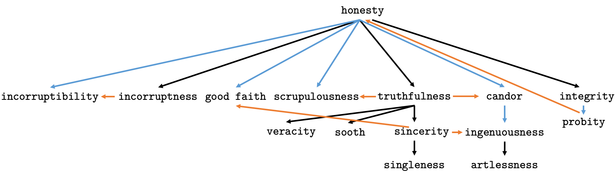
Figure 6: A fragment of a subtree from the WordNet  hierarchy. Orange indicates incorrectly predicted edges and blue indicates edges that were missed.

Some trees in the gold WordNet hierarchy contain ambiguous edges. Figure 5 shows one example. In this subtree, the model predicts arteriography as a sibling of arthrography rather than as its child. The definitions of these two terms suggest why the model may have considered these terms as siblings: arteriograms produce images of arteries while arthrograms produce images of the inside of joints. In Figure 6 we show a second example of an ambiguous tree. The model predicts good faith as a child of sincerity rather than as a child of honesty, but the correct hypernymy relation between these terms is unclear to the authors, even after referencing multiple dictionaries.

These examples point to the potential of augmenting or improving the relations listed in WordNet using semi-automatic methods.

5.6 Web-Retrieved Glosses Are Beneficial When They Contain Lexical Overlap

We compare the predictions of RoBERTa-Large, with and without web glosses, to understand what kind of glosses help. We split the parenthood edges in the gold trees into two groups based on the glosses: (1) lexical overlap (the parent term appears in the child gloss and/or the child term appears in the parent gloss) and (2) no lexical overlap (neither the parent term nor the child term appears in the other term’s gloss). We find that for edges in the “lexical overlap" group, glosses increase the recall of the gold edges from 60.9 to 67.7. For edges in the “no lexical overlap" group, retrieval decreases the recall (edge recall changes from 32.1 to 27.3).

5.7 Pretraining and Tree Reconciliation Both Contribute to Taxonomy Construction

We performed an ablation study in which we ablated either the pretrained language models for the parenthood prediction step or we ablated the tree reconciliation step. We ablated the pretrained language models in two ways. First, we used a one-layer LSTM on top of GloVe vectors instead of a pretrained language model as the input to the finetuning step, and then performed tree reconciliation as before. Second, we used a randomly initialized RoBERTa-Large model in place of a pretrained network, and then performed tree reconciliation as before. We ablated the tree reconciliation step by substituting the graph-based reconciliation step with a simpler threshold step, where we output a parenthood-relation between all pairs of words with softmax score greater than 0.5. We used the parenthood prediction scores from the fine-tuned RoBERTa-Large model, and substituted tree reconciliation with thresholding.

	P	R	F1
RoBERTa-Large	71.2	65.9	67.4
w/o tree reconciliation	70.8	45.8	51.1
RoBERTa-Random-Init	32.6	28.2	29.3
LSTM GloVe	32.5	23.6	26.6

Table 6: Ablation study. Pretraining and tree reconciliation both contribute to taxonomy construction.

In Table 6, we show the results of our ablation experiments. These results show that both steps (using pretrained language models for parenthood-prediction and performing tree reconciliation) are important for taxonomy construction. Moreover, these results show that the incorporation of a new information source (knowledge learned by pretrained language models) produces the majority of the performance gains.

5.8 Models Struggle to Generalize to Large Taxonomies

To test generalization to large subtrees, we tested our models on the English environment and science taxonomies from SemEval-2016 Task 13 (Bordea et al., 2016a). Each of these taxonomies consists of a single large taxonomic tree with between 125 and 452 terms. Following Mao et al. (2018) and Shang et al. (2020), we used the medium-sized trees from Bansal et al. (2014) to train our models. During training, we excluded all medium-sized trees from the Bansal et al. (2014) dataset that overlapped with the terms in the SemEval-2016 Task 13 environment and science taxonomies.

In Table 7 we show the performance of the RoBERTa-Large CTP model. We show the Edge-F1 score rather than the Ancestor-F1 score in order to compare to previous work. Although the CTP model outperforms previous work in constructing medium-sized taxonomies, this model is limited in its ability to generalize to large taxonomies. Future work can incorporate modeling of the global tree structure into CTP.

Dataset	Model	P	R	F1
Science (Averaged)	CTP	29.4	28.8	29.1
	Mao et al. (2018)	37.9	37.9	37.9
	Shang et al. (2020)	84.0	30.0	44.0
Environment (Eurovoc)	CTP	23.1	23.0	23.0
	Mao et al. (2018)	32.3	32.3	32.3
	Shang et al. (2020)	89.0	24.0	37.0

Table 7: Generalization to large taxonomic trees. Models trained on medium-sized taxonomies generalize poorly to large taxonomies. Future work can improve the usage of global tree structure with CTP.

6 Related Work

Taxonomy induction has been studied extensively, with both pattern-based and distributional approaches. Typically, taxonomy induction involves hypernym detection, the task of extracting candidate terms from corpora, and hypernym organization, the task of organizing the terms into a hierarchy.

While we focus on hypernym organization, many systems have studied the related task of hypernym detection. Traditionally, systems have used pattern-based features such as Hearst patterns to infer hypernym relations from large corpora (e.g. Hearst, 1992; Snow et al., 2005; Kozareva and Hovy, 2010). For example, Snow et al. (2005) propose a system that extracts pattern-based features from a corpus to predict hypernymy relations between terms. Kozareva and Hovy (2010) propose a system that similarly uses pattern-based features to predict hypernymy relations, in addition to harvesting relevant terms and using a graph-based longest-path approach to construct a legal taxonomic tree.

Later work suggests that, for hypernymy detection tasks, pattern-based approaches outperform those based on distributional models (Roller et al., 2018). Subsequent work pointed out the sparsity that exists in pattern-based features derived from corpora, and showed that combining distributional and pattern-based approaches can improve hypernymy detection by addressing this problem (Yu et al., 2020).

In this work we consider the task of organizing a set of terms into a medium-sized taxonomic tree. Bansal et al. (2014) treat this as a structured learning problem and use belief propagation to incorporate siblinghood information. Mao et al. (2018) propose a reinforcement learning based approach that combines the stages of hypernym detection and hypernym organization. In addition to the task of constructing medium-sized WordNet subtrees, they show that their approach can leverage global structure to construct much larger taxonomies from the SemEval-2016 Task 13 benchmark dataset, which contain hundreds of terms (Bordea et al., 2016b). Shang et al. (2020) apply graph neural networks and show that they improve performance in constructing large taxonomies in the SemEval-2016 Task 13 dataset.

Another relevant line of work involves extracting structured declarative knowledge from pretrained language models. For instance, Bouraoui et al. (2019) showed that a wide range of relations can be extracted from pretrained language models such as BERT. Our work differs in that we consider tree structures and incorporate web glosses. Bosselut et al. (2019) use pretrained models to generate explicit open-text descriptions of commonsense knowledge. Other work has focused on extracting knowledge of relations between entities (Petroni et al., 2019; Jiang et al., 2020). Blevins and Zettlemoyer (2020) use a similar approach to ours for word sense disambiguation, and encode glosses with pretrained models.

7 Discussion

Our experiments show that pretrained language models can be used to construct taxonomic trees. Importantly, the knowledge encoded in these pretrained language models can be used to construct taxonomies without additional web-based information. This approach produces subtrees with higher mean $F_{1}$ scores than previous approaches, which used information from web queries.

When given web-retrieved glosses, pretrained language models can produce improved taxonomic trees. The gain from accessing web glosses shows that incorporating both implicit knowledge of input terms and explicit textual descriptions of knowledge is a promising way to extract relational knowledge from pretrained models. Error analyses suggest specific avenues of future work, such as improving predictions for subtrees corresponding to abstractions, or explicitly modeling the global structure of the subtrees.

Experiments on aligned multilingual WordNet  datasets emphasize that more work is needed in investigating the differences between taxonomic relations in different languages, and in improving pretrained language models in non-English languages. Our results provide strong baselines for future work on constructing taxonomies for different languages.

8 Ethical Considerations

While taxonomies (e.g., WordNet) are often used as ground-truth data, they have been shown to contain offensive and discriminatory content (e.g., Broughton, 2019). Automatic systems created by pretrained language models can reflect and exacerbate the biases contained by their training corpora. More work is needed to detect and combat biases that arise when constructing and evaluating taxonomies.

Furthermore, we used previously constructed alignments to extend our results to wordnets in multiple languages. While considering English WordNet as the basis for the alignments allows for convenient comparisons between languages and is the standard method for aligning wordnets across languages, continued use of these alignments to evaluate taxonomy construction imparts undue bias towards conceptual relations found in English.

9 Acknowledgements

We thank the members of the Berkeley NLP group and the anonymous reviewers for their insightful feedback. CC and KL are supported by National Science Foundation Graduate Research Fellowships. This research has been supported by DARPA under agreement HR00112020054. The content does not necessarily reflect the position or the policy of the government, and no official endorsement should be inferred.

Appendix

Language-Specific Pretrained Models

We used pretrained models from the following sources:
https://github.com/codegram/calbert,
https://github.com/google-research/bert/blob/master/multilingual.md (Devlin et al., 2019),
http://turkunlp.org/FinBERT/ (Virtanen et al., 2019),
https://github.com/dbmdz/berts,
https://github.com/wietsedv/bertje (de Vries et al., 2019),
https://huggingface.co/dkleczek/bert-base-polish-uncased-v1,
https://github.com/neuralmind-ai/portuguese-bert,
https://github.com/dccuchile/beto/blob/master/README.md (Cañete et al., 2020)

Multilingual WordNet Dataset Statistics

Table 8 details the datasets we created by using synset alignments to the English dataset proposed in Bansal et al. (2014). The data construction method is described in Section 3.1.

	Num			Average
	Trees			Nodes per Tree
	Train	Dev	Test	Train	Dev	Test
ca	391	94	90	9.2	9.3	8.7
zh	216	48	64	10.0	12.4	9.2
en	533	114	114	19.7	20.3	19.8
fi	532	114	114	17.8	18.8	18.1
fr	387	82	76	8.7	9.1	8.3
it	340	85	75	6.3	7.2	6.2
nl	308	58	64	6.6	6.7	6.3
pl	283	73	72	7.7	8.0	7.4
pt	347	68	77	7.1	8.2	7.2
es	280	60	60	6.5	6.1	5.8

Table 8: Dataset Statisics. For each language, we show the number of train, dev, and test subtrees that remain after the subsetting procedure described in Section 3.1.1. In addition, we show the mean number of nodes per tree in each language. We use ISO 639-1 language acronyms.

Ablation Results

Table 9 shows the results for the learning rate trials for the ablation experiment.

	1e-5	1e-6	1e-7
RoBERTa-Large	59.5	67.3	60.7
w/o tree reconciliation	38.6	51.2	18.2
RoBERTa-Random-Init	17.4	26.4	27.0

Table 9: Dev F1 Scores for Different Learning Rates, Ablation Experiments .

Table 10 shows the results for the test trials for the ablation experiment.

	Run 0	Run 1	Run 2
RoBERTa-Large	67.1	67.3	67.7
w/o tree reconciliation	51.2	51.4	50.6
RoBERTa-Random-Init	27.0	29.9	31.1
LSTM GloVe	24.6	27.7	27.6

Table 10: Dev F1 Scores for Three Trials, Ablation Experiments .

SemEval Results

Dataset	Run 0	Run 1	Run 2
Science (Combined)	28.6	31.7	25.1
Science (Eurovoc)	26.6	37.1	31.5
Science (WordNet)	26.5	28.8	25.8
Environment (Eurovoc)	23.4	21.5	24.2

Table 11: Test F1 Scores for Three Trials, Semeval. We show the Edge-F1 score rather than the Ancestor-F1 score in order to compare to previous work.

Table 11 shows the results for the test trials for the SemEval experiment. These results all use the RoBERTa-Large model in the parenthood prediction step.

Random Baseline for Multilingual WordNet Datasets

To compute the random baseline in each language, we randomly construct a tree containing the nodes in each test tree and compute the ancestor precision, recall and $F_{1}$ score on the randomly constructed trees. We include the $F_{1}$ scores for three trials in Table 12.

Model	Run 0	Run 1	Run 2
Catalan	19.7	19.1	21.2
Chinese	23.5	26.8	27.0
English	8.1	8.9	9.7
Finnish	10.6	10.0	9.8
French	22.1	24.7	19.4
Italian	28.0	27.1	31.6
Dutch	29.7	27.9	22.8
Polish	20.5	22.1	27.5
Portuguese	27.9	28.1	22.2
Spanish	32.6	24.1	24.3

Table 12: Test F1 Scores for Three Trials Using a Random Baseline.

Subtree Construction Results, English WordNet

Table 13 shows the results for the learning rate trials for the English WordNet experiment.

Model	1e-5	1e-6	1e-7
BERT	60.0	63.3	60.7
BERT-Large	59.5	67.3	65.8
RoBERTa-Large	56.3	67.1	65.5
RoBERTa-Large
(Web-retrieved Glosses)	58.6	71.5	64.7
RoBERTa Large
(WordNet Glosses)	63.0	83.7	82.9

Table 13: Dev Results for Different Learning Rates, English Models. We highlight in bold the best learning rate for each model.

Table 14 shows the results for the test trials for the English WordNet experiment.

Model	Run 0	Run 1	Run 2
BERT	53.6	54.0	52.5
BERT-Large	58.9	61.5	63.8
RoBERTa-Large	62.9	64.2	63.3
RoBERTa-Large
(Web-retrieved
glosses)	66.6	66.3	67.1
RoBERTa-Large
(WordNet glosses)	82.4	84.0	83.2

Table 14: Test F1 Scores for Three Trials, English.

Subtree Construction Results, Multilingual WordNet

Table 15 shows the results for the learning rate trials for the non-English WordNet experiments.

Language	Model	1e-5	1e-6	1e-7
Catalan	Calbert	39.9	37.9	24.5
	mBERT	39.7	43.5	32.6
Chinese	Chinese BERT	56.9	59.0	54.3
	mBERT	57.4	60.6	44.7
Finnish	FinBERT	45.6	50.1	47.0
	mBERT	24.6	30.2	28.9
French	French BERT	48.9	50.6	46.9
	mBERT	40.3	41.1	32.5
Italian	Italian BERT	52.6	52.2	46.9
	mBERT	50.7	51.8	41.3
Dutch	BERTje	49.0	48.8	38.1
	mBERT	44.9	44.5	32.9
Polish	Polbert	54.2	52.9	48.2
	mBERT	53.0	50.7	36.4
Portuguese	BERTimbau	51.2	52.0	42.1
	mBERT	38.5	37.8	28.0
Spanish	BETO	56.7	57.4	52.8
	mBERT	49.5	41.5	40.4

Table 15: Dev Results for Different Learning Rates, Multilingual. We highlight in bold the best learning rate for each model.

Table 16 shows the results for the test trials for the non-English WordNet experiments.

Language	Model	Run 0	Run 1	Run 2
Catalan	Calbert	36.5	34.1	33.6
	mBERT	39.4	41.8	32.7
Chinese	Chinese BERT	57.1	62.3	56.8
	mBERT	55.2	59.4	58.0
Finnish	FinBERT	43.6	44.6	43.2
	mBERT	25.5	26.3	26.7
French	French BERT	47.5	49.5	50.4
	mBERT	41.0	40.9	38.9
Italian	Italian BERT	43.2	47.2	47.8
	mBERT	42.9	43.6	49.3
Dutch	BERTje	43.8	44.9	42.4
	mBERT	35.9	33.0	27.1
Polish	Polbert	51.2	49.9	47.3
	mBERT	40.1	42.0	41.5
Portuguese	BERTimbau	57.6	57.4	55.8
	mBERT	38.4	38.2	34.3
Spanish	BETO	50.8	53.4	50.9
	mBERT	48.7	49.3	44.0

Table 16: Test F1 Scores for Three Trials, Multilingual.

Table 17 shows the results for all tested models for the non-English WordNet experiments.

Language	Model	P	R	F1
Catalan	Calbert	39.3	32.4	34.7
	mBERT	38.7	39.7	38.0
Chinese	Chinese BERT	62.2	57.3	58.7
	mBERT	61.9	56.0	57.5
Finnish	FinBERT	47.9	42.6	43.8
	mBERT	29.6	25.4	26.2
French	French BERT	51.3	49.1	49.1
	mBERT	43.3	40.0	40.3
Italian	Italian BERT	48.3	45.5	46.1
	mBERT	47.6	44.6	45.3
Dutch	BERTje	44.6	44.8	43.7
	mBERT	34.3	31.6	32.0
Polish	Polbert	51.9	49.7	49.5
	mBERT	43.7	41.4	41.2
Portuguese	BERTimbau	59.3	57.1	56.9
	mBERT	38.7	38.2	37.0
Spanish	BETO	53.1	51.7	51.7
	mBERT	47.3	49.4	47.3

Table 17: Multilingual WordNet Test Results. We use ISO 639-1 acronyms to indicate languages.

References

- Agirre et al. (2011) A. Agirre, Egoitz Laparra, and German Rigau. 2011. Multilingual central repository version 3 . 0 : upgrading a very large lexical knowledge base.
- Bansal et al. (2014) Mohit Bansal, David Burkett, Gerard De Melo, and Dan Klein. 2014. Structured learning for taxonomy induction with belief propagation. In Proceedings of the 52nd Annual Meeting of the Association for Computational Linguistics (Volume 1: Long Papers), pages 1041–1051.
- Bender (2011) Emily M. Bender. 2011. On achieving and evaluating language-independence in nlp. Linguistic Issues in Language Technology, 6.
- Blevins and Zettlemoyer (2020) Terra Blevins and Luke Zettlemoyer. 2020. Moving down the long tail of word sense disambiguation with gloss-informed biencoders. In ACL.
- Bond and Paik (2012) Francis Bond and Kyonghee Paik. 2012. A survey of wordnets and their licenses.
- Bordea et al. (2016a) Georgeta Bordea, Els Lefever, and Paul Buitelaar. 2016a. SemEval-2016 task 13: Taxonomy extraction evaluation (TExEval-2). In Proceedings of the 10th International Workshop on Semantic Evaluation (SemEval-2016), pages 1081–1091, San Diego, California. Association for Computational Linguistics.
- Bordea et al. (2016b) Georgeta Bordea, Els Lefever, and Paul Buitelaar. 2016b. Semeval-2016 task 13: Taxonomy extraction evaluation (texeval-2). In Proceedings of the 10th International Workshop on Semantic Evaluation. Association for Computational Linguistics.
- Bosselut et al. (2019) Antoine Bosselut, Hannah Rashkin, Maarten Sap, Chaitanya Malaviya, A. Çelikyilmaz, and Yejin Choi. 2019. Comet: Commonsense transformers for automatic knowledge graph construction. In ACL.
- Bouraoui et al. (2019) Zied Bouraoui, Jose Camacho-Collados, and Steven Schockaert. 2019. Inducing relational knowledge from bert. arXiv preprint arXiv:1911.12753.
- Broughton (2019) Vanda Broughton. 2019. The respective roles of intellectual creativity and automation in representing diversity: human and machine generated bias.
- Cañete et al. (2020) José Cañete, Gabriel Chaperon, Rodrigo Fuentes, Jou-Hui Ho, Hojin Kang, and Jorge Pérez. 2020. Spanish pre-trained bert model and evaluation data. In PML4DC at ICLR 2020.
- Chu (1965) Yoeng-Jin Chu. 1965. On the shortest arborescence of a directed graph. Scientia Sinica, 14:1396–1400.
- Devlin et al. (2019) J. Devlin, Ming-Wei Chang, Kenton Lee, and Kristina Toutanova. 2019. Bert: Pre-training of deep bidirectional transformers for language understanding. In NAACL-HLT.
- Geiger et al. (2020) A. Geiger, Kyle Richardson, and Christopher Potts. 2020. Neural natural language inference models partially embed theories of lexical entailment and negation. In Proceedings of BlackBoxNLP 2020.
- Hearst (1992) Marti A Hearst. 1992. Automatic acquisition of hyponyms from large text corpora. In Coling 1992 volume 2: The 15th international conference on computational linguistics.
- Hovy et al. (2009) E. Hovy, Zornitsa Kozareva, and E. Riloff. 2009. Toward completeness in concept extraction and classification. In EMNLP.
- Jiang et al. (2020) Zhengbao Jiang, Frank F Xu, Jun Araki, and Graham Neubig. 2020. How can we know what language models know? Transactions of the Association for Computational Linguistics, 8:423–438.
- Joshi et al. (2020) Pratik Joshi, Sebastin Santy, Amar Budhiraja, Kalika Bali, and Monojit Choudhury. 2020. The state and fate of linguistic diversity and inclusion in the nlp world. arXiv preprint arXiv:2004.09095.
- Kozareva and Hovy (2010) Zornitsa Kozareva and Eduard Hovy. 2010. A semi-supervised method to learn and construct taxonomies using the web. In Proceedings of the 2010 conference on empirical methods in natural language processing, pages 1110–1118.
- Lindén and Niemi (2014) Krister Lindén and Jyrki Niemi. 2014. Is it possible to create a very large wordnet in 100 days? an evaluation. Language Resources and Evaluation, 48:191–201.
- Magnini et al. (1994) B. Magnini, C. Strapparava, F. Ciravegna, and E. Pianta. 1994. A project for the construction of an italian lexical knowledge base in the framework of wordnet.
- Mao et al. (2018) Yuning Mao, Xiang Ren, Jiaming Shen, Xiaotao Gu, and Jiawei Han. 2018. End-to-end reinforcement learning for automatic taxonomy induction. In Proceedings of the 56th Annual Meeting of the Association for Computational Linguistics (Volume 1: Long Papers), pages 2462–2472, Melbourne, Australia. Association for Computational Linguistics.
- Mielke (2016) Sabrina J. Mielke. 2016. Language diversity in acl 2004 - 2016.
- Miller (1998) George A Miller. 1998. WordNet: An electronic lexical database. MIT press.
- de Paiva and Rademaker (2012) Valeria de Paiva and Alexandre Rademaker. 2012. Revisiting a brazilian wordnet. Scopus.
- Pennington et al. (2014) Jeffrey Pennington, Richard Socher, and Christopher D Manning. 2014. Glove: Global vectors for word representation. In Proceedings of the 2014 conference on empirical methods in natural language processing (EMNLP), pages 1532–1543.
- Peters et al. (2019) Matthew E Peters, Mark Neumann, Robert Logan, Roy Schwartz, Vidur Joshi, Sameer Singh, and Noah A Smith. 2019. Knowledge enhanced contextual word representations. In Proceedings of the 2019 Conference on Empirical Methods in Natural Language Processing and the 9th International Joint Conference on Natural Language Processing (EMNLP-IJCNLP), pages 43–54.
- Petroni et al. (2019) Fabio Petroni, Tim Rocktäschel, Sebastian Riedel, Patrick Lewis, Anton Bakhtin, Yuxiang Wu, and Alexander Miller. 2019. Language models as knowledge bases? In Proceedings of the 2019 Conference on Empirical Methods in Natural Language Processing and the 9th International Joint Conference on Natural Language Processing (EMNLP-IJCNLP), pages 2463–2473.
- Piasecki et al. (2009) M. Piasecki, Stanisław Szpakowicz, and Bartosz Broda. 2009. A wordnet from the ground up.
- Postma et al. (2016) Marten Postma, Emiel van Miltenburg, Roxane Segers, Anneleen Schoen, and Piek Vossen. 2016. Open Dutch WordNet. In Proceedings of the Eight Global Wordnet Conference, Bucharest, Romania.
- Roller et al. (2018) Stephen Roller, Douwe Kiela, and Maximilian Nickel. 2018. Hearst patterns revisited: Automatic hypernym detection from large text corpora. In Proceedings of the 56th Annual Meeting of the Association for Computational Linguistics (Volume 2: Short Papers), pages 358–363, Melbourne, Australia. Association for Computational Linguistics.
- Sagot (2008) Benoît Sagot. 2008. Building a free french wordnet from multilingual resources.
- Shang et al. (2020) Chao Shang, Sarthak Dash, Md Faisal Mahbub Chowdhury, Nandana Mihindukulasooriya, and Alfio Gliozzo. 2020. Taxonomy construction of unseen domains via graph-based cross-domain knowledge transfer. In Proceedings of the 58th Annual Meeting of the Association for Computational Linguistics, pages 2198–2208.
- Snow et al. (2005) Rion Snow, Daniel Jurafsky, and Andrew Y Ng. 2005. Learning syntactic patterns for automatic hypernym discovery. In Advances in neural information processing systems, pages 1297–1304.
- Talmor et al. (2020) Alon Talmor, Oyvind Tafjord, P. Clark, Y. Goldberg, and Jonathan Berant. 2020. Teaching pre-trained models to systematically reason over implicit knowledge. ArXiv, abs/2006.06609.
- Virtanen et al. (2019) A. Virtanen, J. Kanerva, Rami Ilo, Jouni Luoma, Juhani Luotolahti, T. Salakoski, F. Ginter, and Sampo Pyysalo. 2019. Multilingual is not enough: Bert for finnish. ArXiv, abs/1912.07076.
- de Vries et al. (2019) Wietse de Vries, Andreas van Cranenburgh, Arianna Bisazza, Tommaso Caselli, Gertjan van Noord, and M. Nissim. 2019. Bertje: A dutch bert model. ArXiv, abs/1912.09582.
- Wang and Bond (2013) Shan Wang and Francis Bond. 2013. Building the chinese open wordnet (cow): Starting from core synsets.
- Wolf et al. (2019) Thomas Wolf, Lysandre Debut, Victor Sanh, Julien Chaumond, Clement Delangue, Anthony Moi, Pierric Cistac, Tim Rault, Rémi Louf, Morgan Funtowicz, et al. 2019. Huggingface’s transformers: State-of-the-art natural language processing. ArXiv, pages arXiv–1910.
- Yang and Wu (2012) CheYu Yang and Shih-Jung Wu. 2012. Semantic web information retrieval based on the wordnet. International Journal of Digital Content Technology and Its Applications, 6:294–302.
- Yu et al. (2020) Changlong Yu, Jialong Han, Peifeng Wang, Yangqiu Song, Hongming Zhang, Wilfred Ng, and Shuming Shi. 2020. When hearst is not enough: Improving hypernymy detection from corpus with distributional models. In Proceedings of the 2020 conference on empirical methods in natural language processing (EMNLP).