Fluid viscoelasticity triggers fast transitions of a Brownian particle in a double well optical potential

Abstract

Thermally activated transitions are ubiquitous in nature, occurring in complex environments which are typically conceived as ideal viscous fluids. We report the first direct observations of a Brownian bead transiting between the wells of a bistable optical potential in a viscoelastic fluid with a single long relaxation time. We precisely characterize both the potential and the fluid, thus enabling a neat comparison between our experimental results and a theoretical model based on the generalized Langevin equation. Our findings reveal a drastic amplification of the transition rates compared to those in a Newtonian fluid, stemming from the relaxation of the fluid during the particle crossing events.

Understanding the role of fluctuations in the dynamics of nonlinear systems with multiwell energy landscapes is of paramount importance in many disciplines of both fundamental and applied sciences Hänggi et al. (1990); Mel’nikov (1991a). For instance, it has been recognized that thermal noise is responsible for the activation of transitions in a wide variety of processes at mesoscopic scale, such as the magnetization reversals in thin films Koch et al. (2000), molecular reactions García-Müller et al. (2008), protein folding Chung et al. (2009), colloid adsorption at fluid-fluid interfaces Boniello et al. (2015), drug binding Bernetti et al. (2019), photochemical isomerization Fleming et al. (1986), to name but a few. The transition rates in such situations are well described by Kramer’s escape rate theory Kramers (1940), which is based on the dynamics of a Brownian particle in a metastable state, coupled to its environment through a constant drag coefficient, $\gamma_{0}$, and thermal white noise. In particular, in the overdamped limit and in one dimension, the mean time to cross a potential barrier of height $U$, is given by

$$\tau_{\mathrm{K}}=\frac{2\pi\gamma_{0}}{\sqrt{|\kappa_{\mathrm{S}}|\kappa_{\mathrm{W}}}}\exp\left(\frac{U}{k_{B}T}\right),$$ (1)

where $k_{B}$ is the Boltzmann constant, $T$ is the environment temperature, and $\kappa_{\mathrm{W}}>0$ and $\kappa_{\mathrm{S}}<0$ are the local curvatures or stiffnesses of the potential well where the particle initially equilibrates, and of the barrier, respectively. Eq. (1) has been experimentally verified by directly visualizing the motion of colloidal particles in water in bistable optical potentials Simon and Libchaber (1992); McCann et al. (1999). Optical trapping experiments have quantitatively elucidated further aspects predicted by numerous noise-activated escape theories  Hänggi et al. (1990); Kramers (1940); Landauer and Swanson (1961); Grote and Hynes (1981); Pollak (1986); Pollak et al. (1989); Mel’nikov (1991b), such as Maxwell-like relations Wu et al. (2009), stochastic transitions in periodic potentials Šiler and Zemánek (2010), Kramers turnover in the intermediate underdamped regime Rondin et al. (2017), escape-rate optimization by energy-landscape shaping Chupeau et al. (2020), and very recently, the accurate characterization of the transition path dynamics Zijlstra et al. (2020).

An important issue that arises when measuring barrier-crossing rates in multidimensional systems, e.g., conformational changes of biomolecules Chung et al. (2009, 2015); Truex et al. (2015); Neupane et al. (2016); Hoffer et al. (2019), is the emergence of memory due to a coarse-grained description of their dynamics Velsko et al. (1983); Cossio et al. (2015); Medina et al. (2018); Satija and Makarov (2019). Such non-Markovian effects were pointed out in a seminal theoretical work by Grote and Hynes in 1980 in the realm of condensed phase reactions Grote and Hynes (1980, 1981), where a frequency-dependent friction was introduced. It predicts an enhancement of the reaction rate with respect to Eq. (1), which was later explored in the context of chemical kinetics Velsko et al. (1983); Bagchi and Oxtoby (1983); García-Müller et al. (2008); Lindenberg et al. (1999). More recently, viscoelastic fluids, widespread in many soft matter systems of biological and technological importance Waigh (2016); Yang et al. (2017); Toschi and Sega (2019), have drawn the attention of many researchers, since they give rise to intriguing phenomena at the mesoscale due to their frequency-dependent flow properties Tung et al. (2017); Narinder et al. (2018); Yuan et al. (2018); Narinder et al. (2019); Plan et al. (2020).

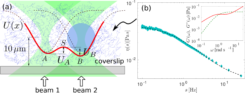
Figure 1: (a) Double-well optical potential. A silica bead with diameter $d_{p}=0.99\,\mu m$ is trapped by two orthogonally-polarized optical tweezers (beams 1 and 2) in a micellar viscoelastic fluid. The resulting potential, $U(x)$ (red solid line), is well described by the sum of two Gaussian functions (dashed curves) according to Eq. (3), giving rise to two stable points (A and B) and a saddle unstable point (S) with barrier heights $U_{A}$ and $U_{B}$ that the particle is able to surmount by thermal fluctuations. The particle is trapped $10\,\mu$m above the bottom coverslip. (b) Viscosity of the micellar solution as a function of the Laplace frequency, obtained by passive microrheology (diamonds). The solid line represents the nonlinear fitting to the Laplace transform of Eq. (2), from which the corresponding storage and loss modulus (dashed and solid line in the inset, respectively) are derived (see Supp. Mat.).

The timescales of Brownian particles embedded in viscoelastic fluids lack a clear-cut separation from timescales of the surroundings due to their complex microstructure, thereby resulting in memory friction with large relaxation times. Their motion is commonly described by the generalized Langevin equation Kubo (1966) with nonequilibrium transient effects that markedly manifest themselves in presence of driving forces Démery et al. (2014); Gomez-Solano and Bechinger (2015); Berner et al. (2018); Mohanty and Zia (2020). Although generalizations of Kramers rate theory involving long-memory friction have been developed in the past in theoretical  Hanggi and Mojtabai (1982); Carmeli and Nitzan (1983); Straub et al. (1986); Talkner and Braun (1988) and numerical works Medina et al. (2018); Kappler et al. (2018); Satija and Makarov (2019); Kappler et al. (2019); Lavacchi et al. (2020), their predictions remain experimentally largely unexplored.

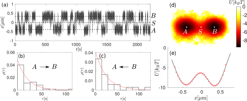
Figure 2: Thermally activated transitions of a colloidal bead ($d_{p}=0.99\,\mu m$), embedded in a micellar viscoelastic fluid, across an optical bistable potential for Exp. I (see main text): (a) time evolution of the trajectory along $x$, (b) normalized histogram of the crossing times from A to B, and (c) from B to A, respectively. The solid red lines depict the maximum likelihood estimation using an exponential model. (d) Experimental 2D potential, and (e) 1D potential across the critical points A, S, B. The dots represent the experimental data while the solid line corresponds to a fitting to Eq. (3).

In this work, we use optical micromanipulation Ashkin (1970); Gieseler et al. (2020); Jones et al. (2015) to show the first experimental realization of thermally-activated transitions of a bead across a bistable potential in a viscoelastic micellar fluid with mono-exponential memory friction . We find a significant increase in the crossing rates over the barrier separating the two local minima, as compared to those in a purely viscous environment. This is in quantitative agreement with a theoretical description based on the generalized Langevin equation, which unveils the mechanism underlying the amplification of the barrier crossing rates.

In our experiments, a spherical silica bead of diameter $d_{p}=0.99\,\mu$m is trapped by a double-well optical potential in a viscoelastic fluid. The potential is sculpted by two optical tweezers ($0.532\,$nm wave length), using a water-immersion objective ($60\times$, 1.2 NA), separated by a distance $\delta_{x}=0.8\pm 0.01\,\mu$m along the focal plane, according to the schematic shown in Fig. 1(a). At this distance the particle can transit between two neatly defined potential wells with characteristic times of the order of seconds. The particle is trapped at temperature $T=22\,^{\circ}$C, and kept at least 10 $\mu$m safe from any hydrodynamic interactions with other particles or with the walls of the sample cell Arzola et al. (2019). The resulting potential is characterized by two stable points (A and B) and an unstable saddle point (S), with barrier heights $U_{A}$ and $U_{B}$, whose values can be adjusted by the total power of the tweezers. We explored three different powers, $0.84\pm 0.05$ mW, $1.11\pm 0.05$ mW and $1.37\pm 0.05$ mW, measured at the objective entrance, which are referred to as experiments I, II and III, respectively. All the experiments were performed using a single bead in a fixed position inside the sample cell, which allowed us to estimate in situ the potential and all the relevant parameters. The uncertainties of such estimates were determined by means of error propagation.

The viscoelastic fluid consists of an equimolar solution of cetylpyridinium chloride and sodium salicylate at $5\,$mM in deionized water, which exhibits a relatively low viscosity and a single relaxation time Ezrahi et al. (2006). At such concentration, the fluid is transparent to visible light. More details about the setup, the sample preparation and the fluid characterization can be found in Supp. Mat. Its relaxation modulus is described by a mono-exponential function Paul et al. (2021), which is a well established model for the linear viscoelasticity of wormlike micelles Hoffmann and Ebert (1988); Fischer and Rehage (1997)

$$G(t)=2\eta_{\infty}\delta(t)+\frac{\eta_{0}-\eta_{\infty}}{\tau_{0}}\exp\left(-\frac{t}{\tau_{0}}\right).$$ (2)

In Eq. (2), $\eta_{\infty}$, $\eta_{0}$, and $\tau_{0}$ represent the solvent viscosity, the zero-shear viscosity and the relaxation time of the fluid Fischer and Rehage (1997); Cates (1996), respectively. In absence of a trapping potential, the particle would freely diffuse in the long-time limit like in a Newtonian fluid with constant viscosity $\eta_{0}$ Grimm et al. (2011); Paul et al. (2018). This provides a criterion to directly compare the barrier crossing process in the viscoelastic fluid with that in a viscous fluid of the same zero-shear viscosity.

In practice, the viscoelastic properties of the micellar fluid were characterized in situ by passive microrheology Squires and Mason (2010); Gieseler et al. (2020) with the same silica bead used in all the double-well experiments. We computed the positional autocorrelation function of the particle trapped by one of the tweezers making up the double-well potential, from which we obtained $\eta_{\infty}=0.0040\pm 0.0001\,\textrm{Pa}\,\textrm{s}$, $\eta_{0}=0.0420\pm 0.0052\,\mathrm{Pa}\,\mathrm{s}$, and $\tau_{0}=1.148\pm 0.067$ s (Method I in Supp. Mat.). Such values are in agreement with those found by a second method based on the motion of a freely-diffusing polystyrene bead of diameter $2\,\mu$m (Method II in Supp. Mat.): $\eta_{\infty}=0.0038\pm 0.0003\,\textrm{Pa}\,\textrm{s}$, $\eta_{0}=0.0453\pm 0.0102\,\mathrm{Pa}\,\mathrm{s}$, and $\tau_{0}=1.206\pm 0.269$ s. In Fig. 1(b) we plot the frequency-dependent viscosity of the fluid, $\eta(s)$, which is directly determined by this method and corresponds to the Laplace transform of Eq. (2). In the inset we also plot the corresponding storage and loss modulus. Our results are in line with reported macroscopic data Handzy and Belmonte (2004), which is not always the case since the response of complex fluids may depend on the size of the microrheological probe Szymański et al. (2006); Makuch et al. (2020).

We track the 2D particle position, $(x,y)$, with a spatial resolution of less than 6 nm at a sampling rate of 1000 Hz using standard videomicroscopy Crocker and Grier (1996); Franklin and Shattuck (2016). Once the particle is confined within the double-well potential, it exhibits thermally-activated transitions between wells A and B through the saddle point S, as illustrated by the intermittent jumps of a typical trajectory plotted in Fig. 2(a). Note that escape events from A to B (A$\rightarrow$B) must be counted separately from those taking place from B to A (B$\rightarrow$A) because optical double wells are in general asymmetric  Simon and Libchaber (1992); McCann et al. (1999); Wu et al. (2009); Zijlstra et al. (2020). Thus, the barrier-crossing time, $\tau$, is defined as the time spent by the particle in metastable equilibrium within a given well plus the time to spontaneously jump over the barrier to finally reach the neighborhood of the contiguous energy minimum. In Figs. 2(b) and (c) we show the normalized histograms of $\tau$ for transitions A$\rightarrow$B and B$\rightarrow$A in Exp. I, respectively. By means of maximum likelihood estimation, we find that the distribution of $\tau$ is well described by $\rho(\tau)=[\tau^{(\textrm{ve})}_{\textrm{exp}}]^{-1}\exp[-\tau/\tau^{(\textrm{ve})}_{\textrm{exp}}]$, with $\tau^{(\textrm{ve})}_{\textrm{exp}}$ the mean crossing time, as depicted by the red solid lines in Figs. 2(b) and (c). Such an exponential behavior suggests that the activated jumps can be considered as a Poisson process Simon and Libchaber (1992). Hence, the asymmetry of the double well in a single experiment allows us to analyze transitions A$\rightarrow$B independently of B$\rightarrow$A, each one characterized by a set of values of the well curvatures and the energy barrier.

The experimental potential is retrieved from the particle trajectories using the equilibrium distribution $\rho(x,y)=\rho_{0}\exp[-U(x,y)/(k_{B}T)]$. As an example, from the data of Exp. I, we obtain the 2D potential $U(x,y)$, plotted in Fig. 2(d). Fig. 2(e) shows the 1D potential across the colinear critical points A, S and B, $U(x)=U(x,y=0)$, where the solid line represents the fitting to the double-Gaussian potential,

$$U(x)=u_{1}\exp\left[{-\frac{(x-\mu_{1})^{2}}{\sigma_{1}^{2}}}\right]+u_{2}\exp\left[-\frac{(x+\mu_{2})^{2}}{\sigma_{2}^{2}}\right]+u_{0},$$ (3)

where $u_{1,2}<0$ correspond to the potentials of each individual tweezers, while $\mu_{1,2}$ and $\sigma_{1,2}$ are their positions and widths, respectively, and $u_{0}$ is a constant energy value. The resulting values of the potential stiffness around the critical points, $\kappa_{\{\mathrm{A},\mathrm{B},\mathrm{S}\}}=\frac{\partial^{2}}{\partial x^{2}}U(x_{\{\mathrm{A},\mathrm{B},\mathrm{S}\}})$, and the energy barriers, $U_{\{\mathrm{A},\mathrm{B}\}}$, for the whole set of experiments are listed in Table S4 in Supp. Mat. The double well is neatly defined only for a small range of separating distances $\delta_{x}$, but in general a third elusive well may appear near the center of the potential Stilgoe et al. (2011); García et al. (2018).

In Fig. 3(a) we plot the experimental mean crossing time, $\tau^{\textrm{(ve)}}_{\textrm{exp}}$, of a bead in the viscoelastic micellar fluid (red squares) and in water (green circles) against Kramer’s theoretical predictions, $\tau_{\textrm{K}}$, given by Eq. (1). While the mean crossing times in water agree well with Kramer’s theory (dotted line), as verified in previous studies Simon and Libchaber (1992); McCann et al. (1999); Zijlstra et al. (2020), significant deviations are observed under viscoelastic conditions. To assess these discrepancies, we focus on the overdamped particle dynamics in the viscoelastic fluid, subjected to the double-well potential, which is described by the generalized Langevin equation

$$\int_{-\infty}^{t}\Gamma(t-s)\dot{x}(s)ds=-U^{\prime}(x(t))+\zeta(t),$$ (4)

where the term on the left-hand side represents the history-dependent friction exerted by the fluid at time $t$, and $\zeta(t)$ is a Gaussian stochastic force accounting for thermal fluctuations. We assume that $\zeta(t)$ satisfies $\langle\zeta(t)\rangle=0$, and $\langle\zeta(t)\zeta(s)\rangle=k_{B}T\Gamma(|t-s|)$ Kubo (1966). Moreover, the Laplace transform of the memory kernel $\Gamma(t)$ in Eq. (4) is related to the frequency-dependent viscosity $\eta(s)$ plotted in Fig. 1(b) via $\tilde{\Gamma}(s)=3\pi d_{p}\eta(s)$. The dissipation at short and long timescales is characterized by the friction coefficients $\gamma_{\infty}=3\pi d_{p}\eta_{\infty}$ and $\gamma_{0}=3\pi d_{p}\eta_{0}$, respectively, whereas elastic effects are quantified by $(\gamma_{0}-\gamma_{\infty})/\tau_{0}$.

Based on these assumptions, we solve numerically Eq. (4) using the experimental information of $U(x)$, $\gamma_{0}$, $\gamma_{\infty}$, and $\tau_{0}$ over a time interval corresponding to the duration of each experiment (40 min). These simulations are performed for 10000 initial equilibrium positions. The details about the simulations are provided in Supp. Mat. The resulting mean crossing times, denoted as $\tau^{(\textrm{ve})}_{\textrm{sim}}$, are plotted in Fig. 3 (blue diamonds). At this point, we find a good agreement between $\tau^{\textrm{(ve)}}_{\textrm{exp}}$ and their corresponding theoretical estimates $\tau^{(\textrm{ve})}_{\textrm{sim}}$, which along with their drastic contrast with $\tau_{\mathrm{K}}$, hint at the importance of viscoelasticity on thermal activation over the barrier.

From Eq. (4), we also derive an explicit expression for the mean barrier-crossing time in the viscoelastic fluid, $\tau^{(\mathrm{ve})}_{\mathrm{th}}$, using Kramer’s rate theory extended to Brownian motion with arbitrarily large memory Hanggi and Mojtabai (1982); Adelman (1976). By computing the diffusive probability current across the potential barrier, $j_{\mathrm{S}}$, and the occupation number in a potential well, $n_{\mathrm{W}}$, we find that $\tau^{(\mathrm{ve})}_{\mathrm{th}}=\frac{n_{\mathrm{W}}}{j_{\mathrm{S}}}$, can be expressed as

$$\tau^{(\mathrm{ve})}_{\mathrm{th}}=\beta\left(\alpha,\frac{\tau_{0}}{\tau_{\mathrm{S}}}\right){\tau}_{\mathrm{K}},$$ (5)

where ${\tau}_{\mathrm{K}}$ is the Kramers time given by Eq. (1), and

$$\beta\left(\alpha,\frac{\tau_{0}}{\tau_{\mathrm{S}}}\right)=\frac{2\alpha}{1-\frac{\tau_{\mathrm{S}}}{\tau_{0}}+\sqrt{\left(1-\frac{\tau_{\mathrm{S}}}{\tau_{0}}\right)^{2}+\frac{4\alpha\tau_{\mathrm{S}}}{\tau_{0}}}},$$ (6)

is a dimensionless factor which accounts for the coupling with the viscoelastic environment. See Supp. Mat. for more details about the derivation. In Eq. (6), $\alpha=\frac{\gamma_{\infty}}{\gamma_{0}}$ is the ratio between the two friction coefficients, whereas $\tau_{\mathrm{S}}=\frac{\gamma_{0}}{|\kappa_{\mathrm{S}}|}$ represents the slowest viscous timescale of the particle when moving in the neighborhood of the saddle point. We realize that for either $\alpha=1$ or $\tau_{0}/\tau_{\mathrm{s}}\rightarrow 0$, $\beta=1$, therefore Eq. (5) reduces to Eq. (1), i.e. the barrier-crossing time in a Newtonian fluid with constant viscosity $\eta_{0}$. On the other hand, for $\gamma_{0}>\gamma_{\infty}$ and $\tau_{0}>0$, which are the conditions describing viscoelastic behavior, it can be checked that $\beta<1$, hence ${\tau}^{(\mathrm{ve})}_{\mathrm{th}}<{\tau}_{\mathrm{K}}$ for all values of the local curvature $\kappa_{\mathrm{S}}$, thereby quantifying the viscoelasticity-induced reduction in the transition times.

In Fig. 3(b) we verify that the experimental values of the mean transition times, $\tau^{(\mathrm{ve})}_{\mathrm{exp}}$ (red squares), and their respective theoretical predictions, $\tau^{(\mathrm{ve})}_{\mathrm{th}}$, are consistent, where the identity (dotted line) represents the ideal prediction by Eq. (5). It should be noted that the numerical values of the mean crossing time, $\tau^{(\textrm{ve})}_{\textrm{sim}}$, and those given by Eq. (5), are in good agreement in spite of their different assumptions. While the numerical results are computed from the finite-time dynamics of a Brownian particle exploring the whole double-well potential, $\tau^{(\mathrm{ve})}_{\mathrm{th}}$ is derived for an ensemble of independent particles starting in equilibrium within a well and then escaping over the barrier. This confirms that the experimental transitions A$\rightarrow$B and B$\rightarrow$A are independent of each other.

Furthermore, in Fig. 4 we plot the ratio $\beta=\tau^{(\textrm{ve})}_{\textrm{exp}}/\tau_{\textrm{K}}$ versus $\tau_{0}/\tau_{\mathrm{S}}$, thus verifying that the coupling of the particle with the viscoelastic surroundings gives rise to a reduction in the mean crossing time in quantitative agreement with Eq. (6). For comparison, we also plot the results of the particle crossing events in water, for which we verify that $\beta\approx 1$, as expected for a Newtonian fluid with constant viscosity ($\alpha=1$ and $\tau_{0}/\tau_{\textrm{S}}\rightarrow 0$). These findings suggest that when the fluid relaxation takes place on a timescale $\tau_{0}\ll\tau_{\mathrm{S}}$, the particle friction around the unstable point S is dominated by the low-frequency values of the viscosity $\eta(s)$ in Fig. 1(b). However, as $\tau_{0}/\tau_{\mathrm{S}}$ increases, the fluid does not have enough time to fully relax before the particle is activated by a thermal fluctuation over the barrier. Hence, the friction experienced by the particle during the escape is strongly affected by higher-frequency components of the viscosity shown in Fig. 1(b). This results in a lower resistance to the particle crossing over the barrier, i.e., $\beta$ decreases monotonically with increasing $\tau_{0}/\tau_{\mathrm{S}}$. Note that under our experimental conditions, the values of $\tau_{\mathrm{S}}$ are comparable to $\tau_{0}$, which allows us to clearly resolve the effect of the fluid viscoelasticity on the escape process of the particle ($\beta\approx 0.2$).

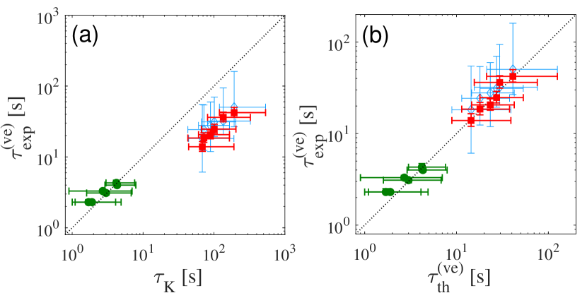
Figure 3: (a) Experimental mean crossing times of the bead in a viscoelastic fluid (red squares) and in water (green circles) versus the Kramer’s prediction for a Newtonian fluid with constant viscosity $\eta_{0}$. Blue diamonds represent the results of the numerical simulations of Eq. (4). The dotted line depicts perfect agreement with Kramer’s theory. (b) Corresponding experimental mean crossing times versus theoretical prediction for a viscoelastic fluid given by Eq (5). The dotted line depicts perfect agreement between experiment and theory.

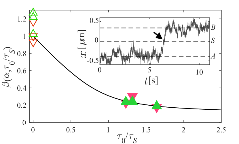
Figure 4: Ratio between the experimental mean crossing time in a viscoelastic fluid and the expected Kramer’s time for the same zero-shear viscosity, as a function of $\tau_{0}/\tau_{\mathrm{S}}$. Filled upward and downward triangles represent transitions A$\rightarrow$B and B$\rightarrow$A in the viscoelastic fluid, while open triangles correspond to transitions A$\rightarrow$B and B$\rightarrow$A in water

. The solid line is the theoretical prediction by Eq. (5). Inset: example of a transition A$\rightarrow$B in the viscoelastic fluid. The arrow depicts the region around S where the particle mobility suddenly rises from $\mu_{\textrm{eff}}\approx\mu_{0}$ to $\mu_{\textrm{eff}}\approx\mu_{\infty}$.

As previously suggested for chemical reactions Grote and Hynes (1981), under non-Markovian conditions activated transitions are triggered by the short-time friction with the solvent. To verify this mechanism in the present case, we estimate the effective particle mobility, $\mu_{\mathrm{eff}}$, from the trajectory of the particle along the barrier crossings, such as the one depicted in the inset of Fig. 4. Then, we compare it with the frequency-dependent particle mobility, which can be derived from Fourier transform of Eq. (4), considering the memory kernel given by Eq. (2),

$$\mu_{\omega}=\frac{\gamma_{0}+\omega^{2}\tau_{0}^{2}\gamma_{\infty}}{\gamma_{0}^{2}+\omega^{2}\tau_{0}^{2}\gamma_{\infty}^{2}}+i\frac{(\gamma_{0}-\gamma_{\infty})\omega\tau_{0}}{\gamma_{0}^{2}+\omega^{2}\tau_{0}^{2}\gamma_{\infty}^{2}}.$$ (7)

Taking into account that the potential around S is harmonic with stiffness $\kappa_{\textrm{S}}$, the mean time to go from a position $x_{\textrm{S}}$ to a neighboring point $x_{\textrm{S}}+\delta$ can be approximated by $\overline{\Delta t}={(\kappa_{\textrm{S}}\mu_{\mathrm{eff}})^{-1}}\ln[1+(\delta/x_{\textrm{S}})]$. Using $\delta=0.15\,\mu$m, for Exp. I, we find the mean effective mobility $\mu_{\mathrm{eff}}\approx 25.7\,\mu\textrm{m}\,\textrm{pN}^{-1}\textrm{s}^{-1}$, which is one order of magnitude greater than the zero-frequency mobility $\mu_{0}=\gamma_{0}^{-1}=2.6\pm 0.3\,\mu\mathrm{m}\,\mathrm{pN}^{-1}\,\mathrm{s}^{-1}$, and very close to the high-frequency mobility $\mu_{\infty}=\gamma_{\infty}^{-1}=26.8\pm 0.7\,\mu\textrm{m}\,p\textrm{N}^{-1}\textrm{s}^{-1}$, described by Eq. (7). This is in stark contrast to the characteristic mobilities in A and B, which for Exp. I are $\mu_{\mathrm{eff}}\approx 2.7\,\mu\textrm{m}\,\textrm{pN}^{-1}\textrm{s}^{-1}$ and $\mu_{\mathrm{eff}}\approx 3.1\,\mu\textrm{m}\,\textrm{pN}^{-1}\textrm{s}^{-1}$, respectively, i.e., closer to $\mu_{0}$. Therefore, unlike activated transition of a particle with constant mobility in a Newtonian fluid, the high-frequency viscosity of a viscoelastic fluid gives rise to a lower friction around the unstable saddle point, thereby enhancing the probability of surmounting the barrier.

In summary, we have investigated the effect of viscoelastic memory friction on the transitions of a micron-sized bead in a double-well optical potential, and in particular, on the mean time that the particle takes to move from one well to the other. Our findings clearly demonstrate that the mean crossing times in a model fluid with mono-exponential memory are shorter than those expected in a Newtonian fluid of similar zero-shear viscosity. This effect was quantified by a factor $\beta\leq 1$ that depends on the fluid properties and on the curvature of the potential barrier, whose values are predicted by a theoretical approach based on the generalized Langevin equation. We show that a non-homogeneous frequency-dependent mobility that drastically increases around the energy barrier is responsible for these fast transitions. This study provides a major understanding of barrier crossing processes under non-Markovian conditions that should impact our comprehension of plenty of transport mechanisms in nature, commonly occurring in non-Newtonian fluids, such as those involving microorganisms and biomolecules Lauga (2020); D’Avino and Maffettone (2015); Kharchenko and Goychuk (2012); Bernheim-Groswasser et al. (2018), as well as activated transitions in other types of non-equilibrium systems with intrinsic memory, e.g. active matter Woillez et al. (2020) and glassy materials Chaki and Chakrabarti (2020). Further experimental and theoretical efforts could help to address other aspects at different physical conditions, such as particle escape over small barriers Abkenar et al. (2017), in complex fluids with non-exponential relaxations Song et al. (2019), or with particles smaller than the characteristic length-scale of the medium Makuch et al. (2020). Finally, this phenomenon can be exploited to envisage new approaches to selectively deliver microscopic assays in artificially generated potential landscapes Zemánek et al. (2019); Arzola et al. (2017, 2011); Lee and Grier (2006); Paterson et al. (2005); MacDonald et al. (2003); Korda et al. (2002); Hänggi and Marchesoni (2009).

*

References

- Hänggi et al. (1990) P. Hänggi, P. Talkner, and M. Borkovec, Rev. Mod. Phys. 62, 251 (1990).
- Mel’nikov (1991a) V. I. Mel’nikov, Physics Reports 209, 1 (1991a), ISSN 0370-1573.
- Koch et al. (2000) R. H. Koch, G. Grinstein, G. A. Keefe, Y. Lu, P. L. Trouilloud, W. J. Gallagher, and S. S. P. Parkin, Phys. Rev. Lett. 84, 5419 (2000).
- García-Müller et al. (2008) P. García-Müller, F. Borondo, R. Hernandez, and R. Benito, Physical review letters 101, 178302 (2008).
- Chung et al. (2009) H. S. Chung, J. M. Louis, and W. A. Eaton, Proceedings of the National Academy of Sciences 106, 11837 (2009), ISSN 0027-8424.
- Boniello et al. (2015) G. Boniello, C. Blanc, D. Fedorenko, M. Medfai, N. B. Mbarek, M. In, M. Gross, A. Stocco, and M. Nobili, Nature Materials 14, 908–911 (2015).
- Bernetti et al. (2019) M. Bernetti, M. Masetti, W. Rocchia, and A. Cavalli, Annual Review of Physical Chemistry 70, 143 (2019).
- Fleming et al. (1986) G. R. Fleming, S. H. Courtney, and M. W. Balk, Journal of Statistical Physics 42, 83 (1986).
- Kramers (1940) H. A. Kramers, Physica 7, 284 (1940), ISSN 0031-8914.
- Simon and Libchaber (1992) A. Simon and A. Libchaber, Physical Review Letters 68, 3375 (1992).
- McCann et al. (1999) L. I. McCann, M. Dykman, and B. Golding, Nature 402, 785 (1999), ISSN 0028-0836.
- Landauer and Swanson (1961) R. Landauer and J. A. Swanson, Phys. Rev. 121, 1668 (1961).
- Grote and Hynes (1981) R. F. Grote and J. T. Hynes, The Journal of Chemical Physics 74, 4465 (1981).
- Pollak (1986) E. Pollak, The Journal of Chemical Physics 85, 865 (1986).
- Pollak et al. (1989) E. Pollak, H. Grabert, and P. Hänggi, The Journal of Chemical Physics 91, 4073 (1989).
- Mel’nikov (1991b) V. Mel’nikov, Physics Reports 209, 1 (1991b), ISSN 0370-1573.
- Wu et al. (2009) D. Wu, K. Ghosh, M. Inamdar, H. J. Lee, S. Fraser, K. Dill, and R. Phillips, Phys. Rev. Lett. 103, 050603 (2009).
- Šiler and Zemánek (2010) M. Šiler and P. Zemánek, New Journal of Physics 12, 083001 (2010).
- Rondin et al. (2017) L. Rondin, J. Gieseler, F. Ricci, R. Quidant, C. Dellago, and L. Novotny, Nature nanotechnology 12, 1130 (2017).
- Chupeau et al. (2020) M. Chupeau, J. Gladrow, A. Chepelianskii, U. F. Keyser, and E. Trizac, Proceedings of the National Academy of Sciences 117, 1383 (2020), ISSN 0027-8424.
- Zijlstra et al. (2020) N. Zijlstra, D. Nettels, R. Satija, D. E. Makarov, and B. Schuler, Phys. Rev. Lett. 125, 146001 (2020).
- Chung et al. (2015) H. S. Chung, S. Piana-Agostinetti, D. E. Shaw, and W. A. Eaton, Science 349, 1504 (2015), ISSN 0036-8075.
- Truex et al. (2015) K. Truex, H. S. Chung, J. M. Louis, and W. A. Eaton, Phys. Rev. Lett. 115, 018101 (2015).
- Neupane et al. (2016) K. Neupane, D. A. N. Foster, D. R. Dee, H. Yu, F. Wang, and M. T. Woodside, Science 352, 239 (2016), ISSN 0036-8075.
- Hoffer et al. (2019) N. Q. Hoffer, K. Neupane, A. G. T. Pyo, and M. T. Woodside, Proceedings of the National Academy of Sciences 116, 8125 (2019), ISSN 0027-8424.
- Velsko et al. (1983) S. P. Velsko, D. H. Waldeck, and G. R. Fleming, The Journal of Chemical Physics 78, 249 (1983).
- Cossio et al. (2015) P. Cossio, G. Hummer, and A. Szabo, Proceedings of the National Academy of Sciences 112, 14248 (2015), ISSN 0027-8424.
- Medina et al. (2018) E. Medina, R. Satija, and D. E. Makarov, The Journal of Physical Chemistry B 122, 11400 (2018), pMID: 30179506.
- Satija and Makarov (2019) R. Satija and D. E. Makarov, The Journal of Physical Chemistry B 123, 802 (2019).
- Grote and Hynes (1980) R. F. Grote and J. T. Hynes, The Journal of Chemical Physics 73, 2715 (1980).
- Bagchi and Oxtoby (1983) B. Bagchi and D. W. Oxtoby, The Journal of Chemical Physics 78, 2735 (1983).
- Lindenberg et al. (1999) K. Lindenberg, A. H. Romero, and J. M. Sancho, Physica D: Nonlinear Phenomena 133, 348 (1999).
- Waigh (2016) T. A. Waigh, Reports on Progress in Physics 79, 074601 (2016).
- Yang et al. (2017) N. Yang, R. Lv, J. Jia, K. Nishinari, and Y. Fang, Annual Review of Food Science and Technology 8, 493 (2017).
- Toschi and Sega (2019) F. Toschi and M. Sega, eds., Numerical Approaches to Complex Fluids (Springer International Publishing, Cham, 2019), pp. 1–34, ISBN 978-3-030-23370-9.
- Tung et al. (2017) C.-k. Tung, C. Lin, B. Harvey, A. G. Fiore, F. Ardon, M. Wu, and S. S. Suarez, Scientific Reports 7, 2045 (2017).
- Narinder et al. (2018) N. Narinder, C. Bechinger, and J. R. Gomez-Solano, Phys. Rev. Lett. 121, 078003 (2018).
- Yuan et al. (2018) D. Yuan, Q. Zhao, S. Yan, S.-Y. Tang, G. Alici, J. Zhang, and W. Li, Lab Chip 18, 551 (2018).
- Narinder et al. (2019) N. Narinder, J. R. Gomez-Solano, and C. Bechinger, New Journal of Physics 21, 093058 (2019).
- Plan et al. (2020) E. L. C. V. M. Plan, J. M. Yeomans, and A. Doostmohammadi, Phys. Rev. Fluids 5, 023102 (2020).
- Kubo (1966) R. Kubo, Reports on Progress in Physics 29, 255 (1966).
- Démery et al. (2014) V. Démery, O. Bénichou, and H. Jacquin, New Journal of Physics 16, 053032 (2014).
- Gomez-Solano and Bechinger (2015) J. R. Gomez-Solano and C. Bechinger, New Journal of Physics 17, 103032 (2015).
- Berner et al. (2018) J. Berner, B. Müller, J. R. Gomez-Solano, M. Krüger, and C. Bechinger, Nature Communications 9, 999 (2018).
- Mohanty and Zia (2020) R. P. Mohanty and R. N. Zia, Journal of Fluid Mechanics 884, A14 (2020).
- Hanggi and Mojtabai (1982) P. Hanggi and F. Mojtabai, Phys. Rev. A 26, 1168 (1982).
- Carmeli and Nitzan (1983) B. Carmeli and A. Nitzan, The Journal of Chemical Physics 79, 393 (1983).
- Straub et al. (1986) J. E. Straub, M. Borkovec, and B. J. Berne, The Journal of Chemical Physics 84, 1788 (1986).
- Talkner and Braun (1988) P. Talkner and H. Braun, The Journal of Chemical Physics 88, 7537 (1988).
- Kappler et al. (2018) J. Kappler, J. O. Daldrop, F. N. Brünig, M. D. Boehle, and R. R. Netz, The Journal of Chemical Physics 148, 014903 (2018).
- Kappler et al. (2019) J. Kappler, V. B. Hinrichsen, and R. R. Netz, Eur. Phys. J. E 42, 119 (2019).
- Lavacchi et al. (2020) L. Lavacchi, J. Kappler, and R. R. Netz, EPL (Europhysics Letters) 131, 40004 (2020).
- Ashkin (1970) A. Ashkin, Phys. Rev. Lett. 24, 156 (1970).
- Gieseler et al. (2020) J. Gieseler, J. R. Gomez-Solano, A. Magazzù, I. P. Castillo, L. P. García, M. Gironella-Torrent, X. Viader-Godoy, F. Ritort, G. Pesce, A. V. Arzola, et al., Advances in Optics and Photonics 13, 74 (2021).
- Jones et al. (2015) P. H. Jones, O. M. Maragò, and G. Volpe, Optical tweezers: Principles and applications (Cambridge University Press, 2015).
- Arzola et al. (2019) A. V. Arzola, L. Chvátal, P. Jákl, and P. Zemánek, Scientific reports 9, 1 (2019).
- Ezrahi et al. (2006) S. Ezrahi, E. Tuval, and A. Aserin, Advances in Colloid and Interface Science 128-130, 77 (2006), ISSN 0001-8686, in Honor of Professor Nissim Garti’s 60th Birthday.
- Paul et al. (2021) S. Paul, N. Narinder, A. Banerjee, K. R. Nayak, J. Steindl, and C. Bechinger, Scientific Reports 11, 2023 (2021).
- Hoffmann and Ebert (1988) H. Hoffmann and G. Ebert, Angewandte Chemie International Edition in English 27, 902 (1988).
- Fischer and Rehage (1997) P. Fischer and H. Rehage, Langmuir 13, 7012 (1997).
- Cates (1996) M. E. Cates, Journal of Physics: Condensed Matter 8, 9167 (1996).
- Grimm et al. (2011) M. Grimm, S. Jeney, and T. Franosch, Soft Matter 7, 2076 (2011).
- Paul et al. (2018) S. Paul, B. Roy, and A. Banerjee, Journal of Physics: Condensed Matter 30, 345101 (2018).
- Squires and Mason (2010) T. M. Squires and T. G. Mason, Annual review of fluid mechanics 42, 413 (2010).
- Handzy and Belmonte (2004) N. Z. Handzy and A. Belmonte, Physical review letters 92, 124501 (2004).
- Szymański et al. (2006) J. Szymański, A. Patkowski, A. Wilk, P. Garstecki, and R. Holyst, The Journal of Physical Chemistry B 110, 25593 (2006), pMID: 17181192.
- Makuch et al. (2020) K. Makuch, R. Hołyst, T. Kalwarczyk, P. Garstecki, and J. F. Brady, Soft Matter 16, 114 (2020).
- Crocker and Grier (1996) J. C. Crocker and D. G. Grier, Journal of colloid and interface science 179, 298 (1996).
- Franklin and Shattuck (2016) S. V. Franklin and M. D. Shattuck, Handbook of granular materials (CRC Press, 2016).
- Stilgoe et al. (2011) A. Stilgoe, N. Heckenberg, T. Nieminen, and H. Rubinsztein-Dunlop, Physical review letters 107, 248101 (2011).
- García et al. (2018) L. P. García, J. D. Pérez, G. Volpe, A. V. Arzola, and G. Volpe, Nature communications 9, 1 (2018).
- Adelman (1976) S. A. Adelman, The Journal of Chemical Physics 64, 124 (1976).
- Abkenar et al. (2017) M. Abkenar, T. H. Gray, and A. Zaccone, Phys. Rev. E 95, 042413 (2017).
- Song et al. (2019) S. Song, S. J. Park, M. Kim, J. S. Kim, B. J. Sung, S. Lee, J.-H. Kim, and J. Sung, Proceedings of the National Academy of Sciences 116, 12733 (2019), ISSN 0027-8424.
- Lauga (2020) E. Lauga, The Fluid Dynamics of Cell Motility, vol. 62 (Cambridge University Press, 2020).
- D’Avino and Maffettone (2015) G. D’Avino and P. L. Maffettone, Journal of Non-Newtonian Fluid Mechanics 215, 80 (2015).
- Kharchenko and Goychuk (2012) V. Kharchenko and I. Goychuk, New Journal of Physics 14, 043042 (2012).
- Bernheim-Groswasser et al. (2018) A. Bernheim-Groswasser, N. S. Gov, S. A. Safran, and S. Tzlil, Advanced Materials 30, 1707028 (2018).
- Woillez et al. (2020) E. Woillez, Y. Kafri, and N. S. Gov, Phys. Rev. Lett. 124, 118002 (2020).
- Chaki and Chakrabarti (2020) S. Chaki and R. Chakrabarti, Soft Matter 16, 7103 (2020).
- Zemánek et al. (2019) P. Zemánek, G. Volpe, A. Jonáš, and O. Brzobohatỳ, Advances in Optics and Photonics 11, 577 (2019).
- Arzola et al. (2017) A. V. Arzola, M. Villasante-Barahona, K. Volke-Sepúlveda, P. Jákl, and P. Zemánek, Physical Review Letters 118, 138002 (2017).
- Arzola et al. (2011) A. V. Arzola, K. Volke-Sepúlveda, and J. L. Mateos, Physical Review Letters 106, 168104 (2011).
- Lee and Grier (2006) S.-H. Lee and D. G. Grier, Physical Review Letters 96, 190601 (2006).
- Paterson et al. (2005) L. Paterson, E. Papagiakoumou, G. Milne, V. Garcés-Chávez, S. A. Tatarkova, W. Sibbett, F. J. Gunn-Moore, P. E. Bryant, A. C. Riches, and K. Dholakia, Applied Physics Letters 87, 123901 (2005), ISSN 0003-6951.
- MacDonald et al. (2003) M. P. MacDonald, G. C. Spalding, and K. Dholakia, Nature 426, 421 (2003), ISSN 1476-4687.
- Korda et al. (2002) P. T. Korda, M. B. Taylor, and D. G. Grier, Physical Review Letters 89, 128301 (2002).
- Hänggi and Marchesoni (2009) P. Hänggi and F. Marchesoni, Rev. Mod. Phys. 81, 56 (2009).