Acousto-optic modulation of a wavelength-scale waveguide

Abstract

We demonstrate a collinear acousto-optic modulator in a suspended film of lithium niobate employing a high-confinement, wavelength-scale waveguide. By strongly confining the optical and mechanical waves, this modulator improves by orders of magnitude a figure-of-merit that accounts for both acousto-optic and electro-mechanical efficiency. Our device demonstration marks a significant technological advance in acousto-optics that promises a novel class of compact and low-power frequency shifters, tunable filters, non-magnetic isolators, and beam deflectors.

I Introduction

Lithium niobate (LN) has played a central role in the development of acousto-optic (AO) devices. In the decades following the initial demonstration of the AO tunable filter Harris et al. (1970), the electrical power consumption of these devices improved from watts to milliwatts through the development of Ti-indiffused and proton-exchange LN optical and surface acoustic wave (SAW) waveguides, and through the development of efficient SAW transducers Ohmachi and Noda (1977); Binh et al. (1980); Smith et al. (1990); Hinkov et al. (1994); Duchet et al. (1995). These waveguides only weakly confine the optical and mechanical fields. The potential for greater confinement and thereby larger interaction strengths is an opportunity to again dramatically improve the efficiency and/or reduce the size of these devices.

In recent years a new LN waveguide technology has emerged that can vastly improve electro-optic, acousto-optic, and nonlinear optical devices. Advances in etch techniques have resulted in low-loss, wavelength-scale optical waveguides Wang et al. (2014) in high-quality, single-crystal films of LN Levy et al. (1998). Owing to their high confinement, these waveguides have powered the development of an array of compact, highly efficient nonlinear devices Chang et al. (2016); Rao et al. (2016); Yu et al. (2019) and modulators Wang et al. (2018); McKenna et al. (2020); Sarabalis et al. (2020a) for classical and quantum applications. In tandem, LN films have been used to realize low-loss, strongly-coupled piezoelectric devices Olsson III et al. (2014); Vidal-Álvarez et al. (2017); Pop et al. (2017); Manzaneque et al. (2019); Sarabalis et al. (2020b); Mayor et al. (2020). We have recently demonstrated that high-confinement waveguides in this platform can be efficiently piezoelectrically transduced Dahmani et al. (2020), and that these transducers can vastly improve the acousto-optic efficiency of nanoscale optomechanical resonators Jiang et al. (2020). For many applications, efficient non-resonant acousto-optic transduction is desired.

Here we demonstrate a collinear acousto-optic mode converter using high-confinement, wavelength-scale waveguides in suspended, X-cut films of LN. After reviewing the physics of these modulators including methods for calculating the optomechanical coupling coefficient $g$ (Section II), we discuss how the optical and mechanical modes can be addressed with AO multiplexers (Section III). We use these multiplexers to realize a frequency-shifting, four-port optical switch near $1550~{}\textrm{nm}$ and $440~{}\textrm{MHz}$. We describe the behavior of this device in Section IV. The efficiency of the modulator is characterized in Section V and used to back out an interaction strength $g/\sqrt{\hbar\Omega}$ of $0.38~{}\textrm{mm}^{-1}\mu\textrm{W}^{-1/2}$ which quantifies the required interaction length and mechanical drive power. Owing to this large $g$, this modulator exhibits a record-low power consumption for its length as seen in Table 2. These modulators are inherently non-reciprocal as demonstrated in Section V where we discuss prospects for using them to make non-magnetic isolators. The results reported here mark a significant advance in guided acousto-optics that could enable a new class of low-power, integrated components.

II Optomechanics in a waveguide

The interactions between light and sound have been studied for a long time Brillouin (1922). Here we review these interactions for the modes of a waveguide Wolff et al. (2015); Sipe and Steel (2016); Van Laer et al. (2016); Eggleton et al. (2019), specifically in the case where sound scatters light between two optical modes. In the context of Brillouin scattering, this is often called inter-modal Kittlaus et al. (2017) or inter-polarization Kang et al. (2011) scattering. In contrast to stimulated Brillouin scattering, here we study how light moves in the presence of a strong mechanical drive, where the light does not affect the dynamics of the sound.

We direct our attention to Figure 1 which shows the optical and mechanical modes of a LN waveguide. The waveguide supports a TE₀ mode with electric field $a_{0}\mathbf{e}_{0}\exp\left(i\beta_{0}z-i\omega_{0}t\right)+\textrm{c.c.}$ and a TE₁ mode with field $a_{1}\mathbf{e}_{1}\exp\left(i\beta_{1}z-i\omega_{1}t\right)+\textrm{c.c.}$. It also supports the fundamental horizontal shear (SH₀) mechanical mode with displacement $b\,\mathbf{u}\exp\left(iKz-i\Omega t\right)+\textrm{c.c.}$ which scatters light between the TE₀ and TE₁ modes. The mode profiles $\mathbf{e}_{i}$ and $\mathbf{u}$ are complex vector fields on the $xy$-plane. They are normalized such that $\left|a_{i}\right|^{2}$ and $\left|b\right|^{2}$ are the photon and phonon number flux with units of Hz.

When the scattering process is phasematched, e.g., $\omega_{1}+\Omega=\omega_{0}$ and $\beta_{1}+K=\beta_{0}$ as shown in Figure 1a, the coefficients $\mathbf{a}(t,z)=\left(a_{0}(t,z),a_{1}(t,z)\right)^{\top}$ obey

$$\left(\mathbf{v}^{-1}\partial_{t}+\partial_{z}\right)\mathbf{a}=-igb\sigma_{x}\mathbf{a}$$ (1)

as shown in Appendix A. Here $\mathbf{v}$ is a diagonal matrix containing the optical group velocities, $g$ is the optomechanical coupling coefficient, and $\sigma_{x}$ is the Pauli-X matrix. In Equation 1, we assume $b$ is real.

In the absence of coupling $g\rightarrow 0$, light in the two modes propagate independently according to a telegrapher equation. When we turn on the coupling, light oscillates between the modes

$$\mathbf{a} =\exp\left(-igbz\sigma_{x}\right)\mathbf{a}_{0}$$

$$=\begin{pmatrix}\cos\zeta&-i\sin\zeta\\ -i\sin\zeta&\cos\zeta\end{pmatrix}\mathbf{a}_{0}$$ (2)

where $\zeta\equiv gbz$ and $\mathbf{a}_{0}$ is vector of the initial coefficients at $z=0$. These steady-state solutions assume $b$ is uniform along the waveguide, but we consider a more general case with loss and detuning in Appendix B. Like a bulk acousto-optic modulator, a waveguide-based modulator is a frequency-shifting switch. When $\zeta=\pi/2$, light initially in mode 1 is converted to mode 2 before being converted back to mode 1 at $\zeta=\pi$.

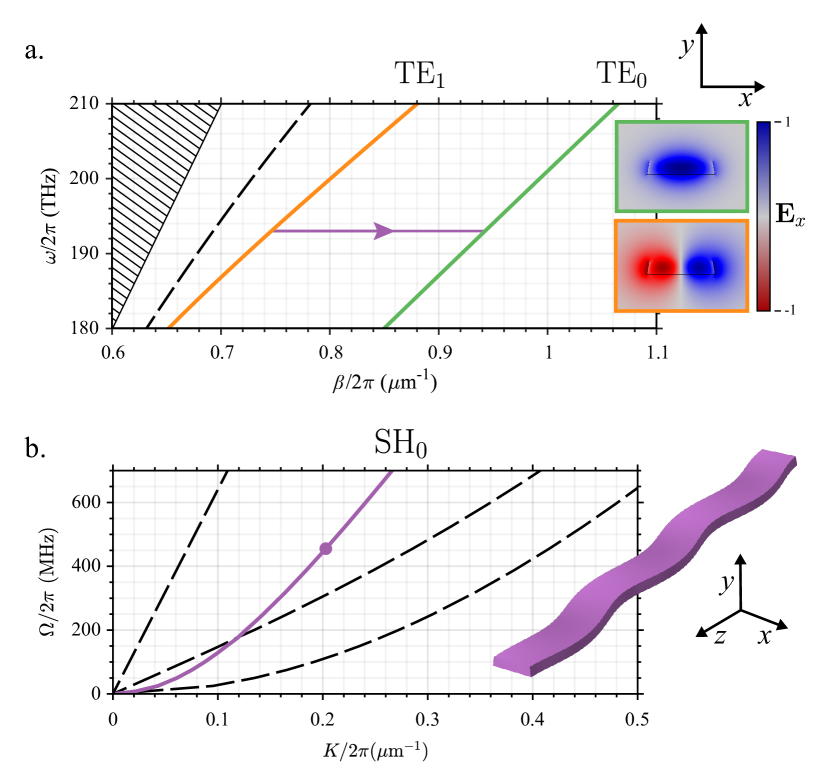
Figure 1: Band Structure a. The LN waveguide investigated supports a TE₀ (green) and TE₁ (orange) mode. The $x$-component of the electric field is plotted showing the TE₁ node on the reflection-symmetry plane. At 193 THz, their wavevectors differ by $K=2\pi\times 0.2~{}\mu\textrm{m}^{-1}$ shown with the purple arrow. b. The fundamental horizontal shear SH₀ mode with this $K$ is plotted alongside the mechanical bands (SH₀ in purple). The mode profiles plotted can be used to compute $g/\sqrt{\hbar\Omega}=1~{}\textrm{mm}^{-1}\mu\textrm{W}^{-1/2}$.

Confining light and sound to a wavelength-scale waveguide enhances the interaction strength $g$ enabling smaller, more efficient devices. This can be seen in the expression for the coupling coefficient from mode 1 into mode 0

$$g_{01}=-\frac{\omega_{0}}{2}\frac{\int\textrm{d}A\;\mathbf{e}_{0}^{*}\delta_{\mathbf{u}}\varepsilon\cdot\mathbf{u}\mathbf{e}_{1}}{\mathcal{P}_{0}\sqrt{\mathcal{P}_{\textrm{m}}/\hbar\Omega}}.$$ (3)

Here $\mathcal{P}_{i}$ is the optical power in mode $i$ when $|a_{i}|^{2}=1$, $\mathcal{P}_{\textrm{m}}$ is the mechanical power when $|b|^{2}=1$, and $\delta_{\mathbf{u}}\varepsilon\cdot\mathbf{u}$ encodes the permittivity shift from the deformation $\mathbf{u}$ as described in Appendix A. First we note how this expression relates to $g$ in Equation 1. By choosing a flux-normalized basis where $\mathcal{P}_{i}=\hbar\omega_{i}$, the coupling takes a Hermitian form $g_{ij}=g_{ji}^{*}$. This can be made real and symmetric by choice of phase of the mode profiles, giving us the $g$ used in equation (1).

Next we consider how $g$ scales with the area of a waveguide. In the limit of high-confinement, small changes to a waveguide’s geometry change its dispersion and the shape of its modes. For fixed $\omega$, $g$ has a complicated dependence on waveguide geometry. When the waves are weakly confined, the numerator in Equation 3, $\mathcal{P}_{0}$, and $\mathcal{P}_{\textrm{m}}$ are approximately proportional to the area of the waveguide $A$. In this regime, the factors of $A$ from the numerator and $P_{0}$ cancel, leaving only $A^{-1/2}$ from $\mathcal{P}_{\textrm{m}}$. Intuitively, it takes more power $\mathcal{P}_{\textrm{m}}$ to deform a larger waveguide by $\mathbf{u}$ which comes at the expense of $g$ and, ultimately, a device’s efficiency. Other three-wave processes like electro-optic and $\chi^{\left(2\right)}$ interactions scale similarly. This motivates the pursuit of high-confinement waveguides for nonlinear and parametric processes like acousto-optics, underlying recent activity in thin-film LN.

We can use Equation 3 to calculate the coupling for the rectangular waveguide studied here. Our waveguide is patterned into X-cut LN and suspended by etching the silicon substrate. It is $1.25~{}\mu\textrm{m}$ wide and 250 nm thick. We define the waveguide in a hydrogen silsesquioxane mask and transfer it to the lithium niobate film with an argon ion mill. This produces a $10^{\circ}$ sidewall-angle that is included in the simulations. The mode profiles plotted in Figure 1 are used to compute the coupling coefficient

$$\frac{g}{\sqrt{\hbar\Omega}}=1.0~{}\frac{1}{\textrm{mm}\sqrt{\mu\textrm{W}}}.$$ (4)

With approximately 40 microwatts of power in the SH₀ mode, the optical wave is completely transfered from the TE₀ to the TE₁ mode (or vice versa) after traveling just $250~{}\mu\textrm{m}$ in the waveguide.

Mode	$n_{\textrm{eff}}$	$n_{\textrm{g}}$
TE0	1.464	2.147
TE1	1.159	2.288

Mode	$2\pi/K$	$v$
SH0	$5.081~{}\mu\textrm{m}$	$3623~{}\textrm{m/s}$

Table 1: The simulated effective and group indices for the optics at 1550 nm, and the wavelength and group velocity for the mechanics that phase-matches these optical modes.

III Addressing the optical and acoustic modes of a waveguide

In order to use these interactions to build devices, we need to efficiently address each of the optical and mechanical modes in our waveguide. To this end we engineer the acousto-optic multiplexer Dostart and Popović (2020) shown in Figure 2. This device separates the TE₀ optical, TE₁ optical, and SH₀ acoustic waves into three ports and couples them off-chip.

Light and sound behave very differently at the boundary of a waveguide. Mechanical energy is only transferred between two bodies if they touch. On the other hand, light can tunnel across a gap between adjacent dielectrics. We can use this fundamental difference when designing a multiplexer, evanescently transferring light between adjacent waveguides without disturbing the mechanics.

The optical mode multiplexer comprises two adiabatic tapers. The first on the left of Figure 2a and closer to the AO waveguide couples to the TE₁ mode and the second to the TE₀ mode. This design is similar to the cascaded mode-injector developed by Chang et al. to use multi-moded waveguides for compact, low-drive power phase shifters Chang et al. (2017). In our coupler, the 1.25 $\mu\textrm{m}$-wide AO waveguide supports a TE₀ and TE₁ mode. The TE₁ mode is close to cutoff and has long, evanescent tails. Starting from the left, a 200 nm-wide coupling waveguide is brought in to a distance 200 nm from the AO waveguide. As the width is increased, the TE₀ mode of the coupling waveguide hybridizes with the TE₁ mode of the AO waveguide, leading to the anti-crossing in Figure 2b near 600 nm. The coupling waveguide is tapered up to $1~{}\mu\textrm{m}$ in width over $25~{}\mu\textrm{m}$ and the AO waveguide’s TE₁ mode is adiabatically transferred into the coupler’s TE₀. The coupler waveguide is then bent away from the AO waveguide and sent the top grating coupler in figure 2a. After coupling out TE₁, the AO waveguide is narrowed to 575 nm such that TE₀ exhibits long, evanescent tails and the process is repeated for the TE₀ mode, this time tapering the coupler from 400 nm to $1~{}\mu\textrm{m}$.

We measure the optical transmission through the device in Figure 3. Our best device exhibited 10 dB isolation, i.e., unintended scatter from the TE₀ (or TE₁) input port to the TE₁ (TE₀) output port. This crosstalk limits the isolation of our AOM. It can be further reduced by optimizing the device, or by actively compensating for crosstalk with an electically tunable feed network Miller (2015).

The silicon substrate is etched away, releasing the LN waveguides such that they support optical and mechanical waves. Releasing the device causes the AO and coupling waveguides to deviate from the plane of the chip by different amounts, separating and decoupling the waveguides. To prevent this, we add 150 nm-wide tethers at the ends of each coupling waveguide. These tethers can scatter mechanical waves in the AO waveguide, counter to the design strategy.

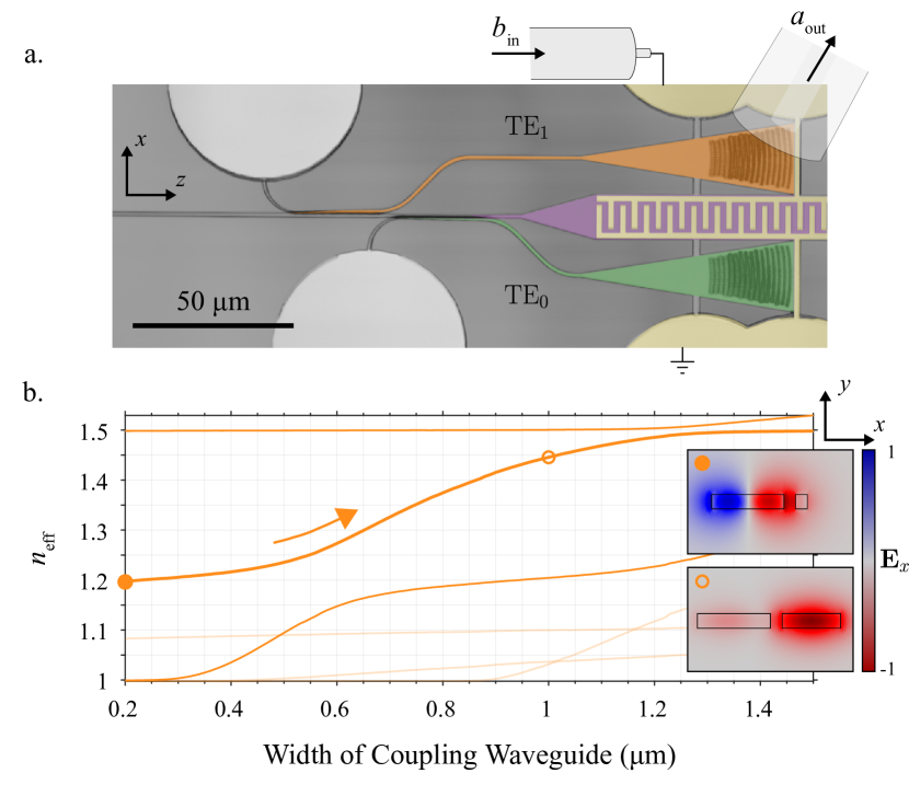
Figure 2: AO multiplexer. a. Light can be injected into the TE₀ and TE₁ modes of the waveguide through the green and orange optical ports, respectively. The SH₀ mechanical mode of the waveguide is excited by the purple piezoelectric transducer. b. The optical mode injectors (TE₁ shown) adiabatically transfer the mode from the waveguide into the TE₀ mode of the coupler by tapering the width of the coupling waveguide.

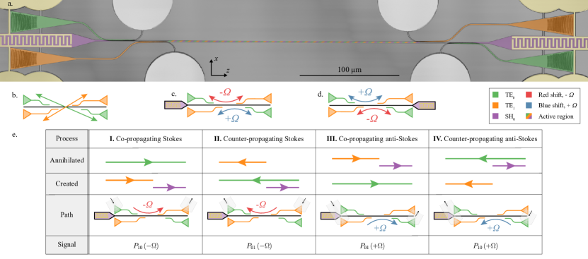
Figure 3: Integrated AOM a. The full modulator comprises two multiplexers described in Section III and a waveguide where the interactions happen, labeled “active region.” It constitutes a four-optical-port, frequency-shifting switch. b. When no phonons are in the waveguide, light propagates along cross-shaped paths. c. When the left transducer is driven, photons that emit/absorb a phonon travel along the top/bottom bar-shaped path. d. If we change the direction of the phonons, the emission/absorption paths are switched. e. We tabulate the four AO processes that govern the device when driven from the left (c.), including the resulting heterodyne signal as described in Section V.

Mechanical waves in the waveguide are coupled out with a piezoelectric transducer after the optical couplers. We adapt the transducer design presented in Ref. Dahmani et al. (2020) for the frequency range of interest. The rescaled design excites the fundamental SH mode with $K=2\pi/5.08~{}\mu\textrm{m}^{-1}$ that can phasematch the TE₀ and TE₁ optical modes at 1550 nm.

We measure the S-matrix of this two-port microwave system on a calibrated probe station and extract the mechanical propagation loss $\gamma=-11.7~{}\textrm{dB/mm}$ and the transmission $|t_{\textrm{b}\mu}|^{2}=-21.9~{}\textrm{dB}$. The peak conductance of these transducers is 2.3 mS and, as a result, 4.3 dB of the insertion loss comes from impedance mismatch. The rest is likely from material damping in the transducer Dahmani et al. (2020).

A more detailed characterization of the multiplexer, including its frequency response, is presented in Appendix C.

IV A waveguide AO modulator

The multiplexers described in the previous section give us access to the optical and mechanical modes of the modulator in Figure 3. All four phase-matched processes — co- and counter-propagating, Stokes and anti-Stokes — are at play in this four-port, frequency-shifting switch.

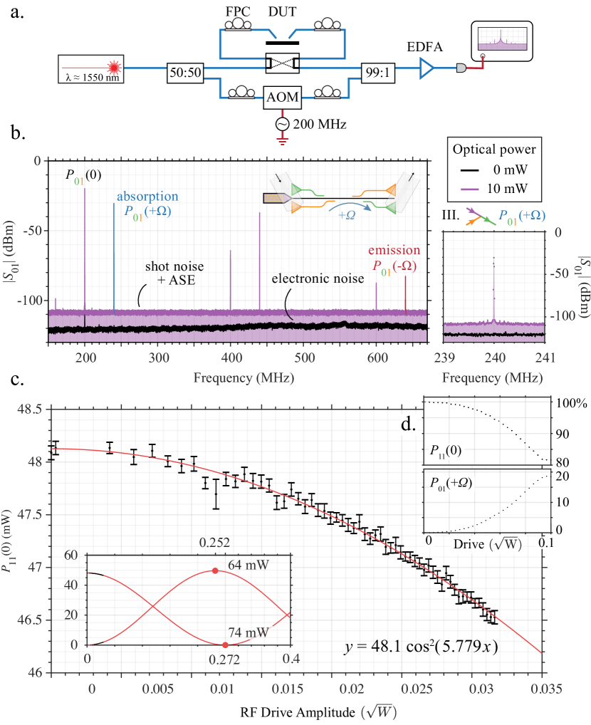
Figure 4: Heterodyne measurements a. Schematic of the optical heterodyne receiver. FPC: fiber polarization controller. DUT: device under test. EDFA: erbium-doped fiber amplifier. b. An example photocurrent spectrum of the co-propagating anti-Stokes process for a 440 MHz drive. The three tones of interest are the unscattered pump, $P_{01}(0)$ at 200 MHz; the absorption signal, $P_{01}(+\Omega)$ at 240 MHz; and the emission signal, $P_{01}(-\Omega)$ at 640 MHz, which is suppressed by over 50 dB. ASE : amplified spontaneous emission. c. Fitting a sinusoid to the pump depletion $P_{11}(0)$, we extrapolate the full-conversion drive power $P_{\pi/2}$ (inset bottom left) which is used to determine $g$. The absorption signal $P_{01}(+\Omega)$ gives us a similar result. d. At higher drive powers, the signal deviates from a sinusoid (Appendix D). We observe up to 18% conversion, where the signals have been normalized by the undepleted pump ($P_{11}(0)$ with the drive off).

First we consider what happens without the mechanical drives. We send light at $\omega$ into the bottom-left grating (orange) which gets injected into the TE₁ mode of the waveguide. With no phonons in the waveguide, the light passes through the device and gets removed by the TE₁ injector, leaving the chip from the top-right grating (orange). The optical paths through an undriven device are shown in Figure 3b.

Now consider the co-propagating anti-Stokes process (Figure 3e. III). Again sending light into the bottom-left, we drive the left transducer with an RF tone at $\Omega$. This sends phonons down the waveguide to the right. Photons in the TE₁ mode of the waveguide absorb co-propagating phonons and scatter into the TE₀ mode. After absorption, their frequency increases to $\omega+\Omega$ and their wavevector increases from $\beta_{1}(\omega)$ to $\beta_{0}(\omega+\Omega)=\beta_{1}(\omega)+K$ (also shown in Figure 1). The TE₀ injector removes these up-shifted photons from the waveguide and they are scattered off-chip by the grating in the bottom-right (green).

If we instead send light into TE₀ from the top-left (green), the co-propagating phonons stimulate emission — instead of absorption — and the incident light scatters into the TE₁ mode at $\omega-\Omega$. The down-shifted light leaves the chip through the top-right grating (orange). This is the co-propagating Stokes process diagrammed in Figure 3e. I.

In addition to the two co-propagating processes described above, there are counter-propagating processes which we probe by sending the optical field from right-to-left (Figure 3e. II, IV). The four processes are summarized in Figure 3c. The co-propagating and counter-propagating Stokes processes — e. I and e. II, respectively — form the top, red-shifted path. The co- and counter-propagating anti-Stokes processes — III and IV — form the bottom, blue-shifted path. When $L_{\textrm{eff}}\gg\Omega^{-1}(v_{1}^{-1}+v_{0}^{-1})^{-1}$, the co- and counter-propagating processes are not simultaneously phase-matched.

Driving the mechanics from the right, i.e., flipping the direction of the phonon, also switches absorption and emission. This gives us Figure 3d which, because of the symmetry of our device, is equivalent to 3c under a $180^{\circ}$ rotation.

We can think of the device as a frequency-shifting optical switch. No matter which direction the phonons are coming from, the mechanical drive switches the device from the “cross” state (b) to the “bar” state (c and d). The direction of the mechanical wave determines which path red-shifts and which path blue-shifts the light.

V Characterizing the modulation

In addition to the mechanical efficiency and attenuation reported in Section III, $g$ is a key figure that determines the modulator’s efficiency. We determine $g$ by measuring the scattered power and pump depletion using the heterodyne setup in Figure 4a. Light in the telecom C band is generated with a Santec TSL-550 laser. It is split with half the light sent to the device and the other half up-shifted by $\Delta\equiv 2\pi\times 200~{}\textrm{MHz}$ using an AOM. The paths are recombined with a 99:1 splitter and sent to an Optilab PD-40-M detector. The photocurrent spectrum $S_{II}[\omega]$ is measured with a Rhode & Schwartz FSW.

A photocurrent spectrum of the co-propagating anti-Stokes process (Figure 3 e. III) is shown in Figure 4b for a drive frequency $\Omega=2\pi\times 440~{}\textrm{MHz}$. There are three important tones in the spectrum : one at $\Delta$ and the other two at $\Omega\pm\Delta$. If the light travels through the device without being scattered by the acoustic wave, its frequency stays the same, leading to the RF tone at 200 MHz. If the light absorbs/emits a phonon from the acoustic field, its frequency is shifted by $\pm 440~{}\textrm{MHz}$, generating the tone at 240/640 MHz. We denote the power in these tones $P_{ij}(\omega^{\prime})$ where $ij$ specifies the optical path TE_j$\rightarrow$TE_i and $\omega+\omega^{\prime}$ is the frequency of the light generating the tone. The power,

$$P_{01}(+\Omega)=Z_{0}\int_{-B/2}^{B/2}\textrm{d}\omega\;S_{II}\left[\Omega-\Delta+\omega\right]$$ (5)

for our example process, is proportional to the optical power emitted from the device. Here $Z_{0}$ is 50 Ohms and $B$ is the integration bandwidth. Each process in Figure 3e is labeled with the resulting $P_{ij}(\omega^{\prime})$.

By fitting the scattered power $P_{10}(+\Omega)$ and pump depletion $P_{11}(0)$, we determine $g$ in way that is insensitive to the calibration of the loss in the optical signal chain (Appendix E). For a phase-matched process, these fits (Figure 4c) give us $gt_{\textrm{b}\mu}L_{\textrm{eff}}/\sqrt{\hbar\Omega}$ where

$$L_{\textrm{eff}}=2\gamma^{-1}\left[1-\exp\left(-\gamma L/2\right)\right]$$ (6)

as described in Appendix B. In Figure 4c, we extrapolate $P_{\pi/2}$, the power it takes to fully swap TE₁$\leftrightarrow$TE₀, which is related to $g$ as

$$gt_{\textrm{b}\mu}L_{\textrm{eff}}\sqrt{\frac{P_{\pi/2}}{\hbar\Omega}}=\frac{\pi}{2}.$$ (7)

After removing the cable loss (0.6 dB), we find

$$\frac{g}{\sqrt{\hbar\Omega}}=0.38~{}\frac{1}{\textrm{mm}\sqrt{\mu\textrm{W}}},$$ (8)

roughly a third the simulated value. This discrepancy is similar to what we have observed for waveguides in LN films on sapphire Sarabalis et al. (2020a) and resonant optomechanical systems in suspended LN films Jiang et al. (2019).

To better understand the different device architectures, we extend the table presented by Smith et al. Smith et al. (1990) to include $t_{\textrm{b}\mu}$, $g$, and recent work with high-confinement waveguides (Table 2). If the conversion efficiency $P_{\pi/2}$ is not directly measured, we extrapolate $P_{\pi/2}$ from low-power measurements of the efficiency. The transducer’s transmission $t_{\textrm{b}\mu}$ is not typically reported. Here we de-embed $t_{\textrm{b}\mu}$ from the two-port S-parameter (Appendix C.2). Without careful analysis, $t_{\textrm{b}\mu}$ is prone to over-estimate. For example, Rayleigh and Bleustein-Gulyaev waves are nearly degenerate for X-cut LN devices Heffner et al. (1988); Frangen et al. (1989); Hinkov and Hinkov (1991); Hinkov et al. (1994) and, if not properly handled, degrade $t_{\textrm{b}\mu}$ without reducing $|S_{21}|$ Duchet et al. (1995). Where we are unable to infer $t_{\textrm{b}\mu}$, we assume $\left|t_{\textrm{b}\mu}\right|^{2}+\left|S_{11}\right|^{2}=1$, which strictly over-estimates $|t_{\textrm{b}\mu}|$. The optomechanical coupling coefficient is inferred from $t_{\textrm{b}\mu}$ and $P_{\pi/2}$ taking into account mechanical loss $\gamma$ where reported. The figure-of-merit $(L/\lambda)^{2}P_{\pi/2}$ is adapted from Smith et al. Smith et al. (1990). It is proportional to $\left|gt_{\textrm{b}\mu}\right|^{-2}$. A low-power, compact modulator requires a low figure-of-merit, i.e., both an efficient transducer and strong photon-phonon interactions.

Work	Year	$\lambda$	$\Omega/2\pi$	$L$	$P_{\pi/2}$	$\gamma$	$\left|t_{\textrm{b}\mu}\right|^{2}$	$g/\sqrt{\hbar\Omega}$	$(L/\lambda)^{2}P_{\pi/2}$	$\eta_{\textrm{max}}$
		(nm)	(MHz)	(mm)	(mW)	(dB/mm)	(dB)	(mm-1 W-1/2)	(MW)	(%)
Harris Harris et al. (1970)	1970	632.8	54	35	$3.64\times 10^{3}$	—	-7.5	0.057	$1.1\times 10^{4}$	95
Ohmachi Ohmachi and Noda (1977)	1977	1150	245.5	4.5	550	—	-20	4.7	8.42	70
Binh Binh et al. (1980)	1980	632.8	550	9	225	—	-25	6.54	45.5	99
Heffner Heffner et al. (1988)	1988	1523	175	25	500	—	-7.0	0.20	135	97
Hinkov Hinkov et al. (1988)	1988	633	191.62	17	400	-0.1	-25	2.6	289	90
Frangen Frangen et al. (1989)	1989	1520	178	9	90	-0.05	-10	1.9	3.16	99
Hinkov Hinkov and Hinkov (1991)	1991	800	355.5	20	19.8	-0.04	-3	0.825	12.4	93
Hinkov Hinkov et al. (1994)	1994	800	365	25	0.5	-0.04	-3	4.2	0.488	100
Duchet Duchet et al. (1995)	1995	1556	170	30	6	—	-3	0.96	2.23	100
Liu Liu et al. (2019)	2019	1510	16,400	0.5	$4.2\times 10^{5}$	—	-15	0.041	46.4	$2.5\times 10^{-4}$
Kittlaus Kittlaus et al. (2020)	2020	1600	3,110	0.240	$4.69\times 10^{3}$	—	-12	5.7	0.105	1
”	”	1525.4	”	0.960	$1.48\times 10^{3}$	—	”	4.5	0.587	13.5
This work	2020	1550	440	0.25	60	-11.7	-21.9	377	$1.6\times 10^{-3}$	18

Table 2: Literature Review We extend the table compiled by Smith et al. Smith et al. (1990) to include estimates for $t_{\textrm{b}\mu}$ and $g$, and recent work on high-confinement waveguide devices. $\eta_{\textrm{max}}$ is the maximum conversion efficiency demonstrated. The values for $g$ are inferred from $P_{\pi/2}$. We account for mechanical propagation loss where reported. High-confinement modulators dramatically improve the figure-of-merit $(L/\lambda)^{2}P_{\pi/2}$.

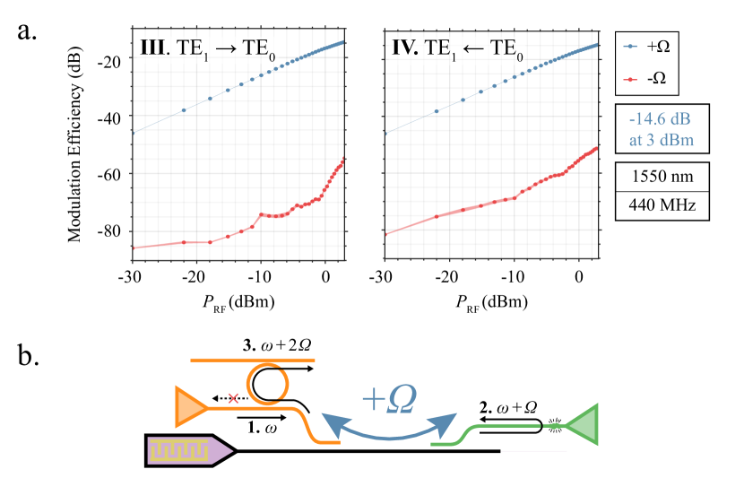
Figure 5: Nonreciprocity a. Light traveling along the bottom path of Figure 3c incurs a $+\Omega$ blue-shift independent of the direction it travels. This is a signature of nonreciprocity. Here modulation efficiency is the scattered power over the undepleted pump, e.g., $P_{01}(+\Omega)$ over $P_{11}(0)$ for III. b. The resulting round-trip frequency-shift can be used to build a frequency-shifting isolator. A ring filter can be added before the AOM to drop reflections.

Acousto-optic modulators are inherently nonreciprocal and can be used to make isolators and circulators to stabilize lasers Smith (1973) and help manage reflections in large photonic circuits. Nonreciprocal components usually employ the magneto-optical effect, motivating the pursuit of thin-film YIG functional layers in silicon photonics Tien et al. (2011); Ghosh et al. (2012). Alternatively, parametric drives like acousto-optics give us a non-magnetic way to build nonreciprocal components  Smith (1973); Heeks and Jackson (1986); O’meara (1988); Li et al. (2014); Peano et al. (2015); Sohn et al. (2018); Sarabalis et al. (2018); Sohn and Bahl (2019); Kittlaus et al. (2020); Williamson et al. (2020).

In these devices, nonreciprocity takes a slightly different form than in a standard isolator. Consider the bottom path in Figure 3c. Light traveling between the TE₁ and TE₀ port absorbs a phonon independent of the direction it travels. This can be seen directly in the path-independent blue-shift measured in Figure 5a. If light takes a round-trip through the device, it absorbs two phonons and returns to a different state.

This round-trip frequency shift is nonreciprocal. It can be used to build the frequency-shifting isolator in Figure 5b Heeks and Jackson (1986). Light back-scattered from, e.g., an imperfect component is shifted by $+2\Omega$ and, as a result, can be dropped by a filter to isolate the input port from reflections. When $L_{\textrm{eff}}\gg v_{1}/2\Omega$, the backwards process is not phase-matched and the reflections are dropped even without a filter Kittlaus et al. (2020). Finally, this device can be cascaded with another AOM to make a fixed-frequency isolator O’meara (1988).

VI Outlook

Building off our recent work on waveguide transduction Dahmani et al. (2020), we demonstrate a compact acousto-optic modulator in a suspended film of X-cut lithium niobate. The modulator comprises a frequency-shifting, four-port optical switch at $440~{}\textrm{MHz}$ and $1550~{}\textrm{nm}$. By employing high-confinement optical and mechanical modes with strong photon-phonon interactions ($g/\sqrt{\hbar\Omega}=0.38~{}\textrm{mm}^{-1}\mu\textrm{W}^{-1/2}$), it exhibits a record-setting figure-of-merit. This device is optically broadband and, as demonstrated, inherently non-reciprocal. We discuss how it can be integrated with an optical filter to implement a fixed-frequency, non-magnetic isolator.

High-confinement waveguides mark a significant advance in the figure-of-merit of collinear AOMs. The device reported here offers a two order-of-magnitude increase in $g$ and a $1,000\times$ improvement in the figure-of-merit over Ti-indiffused and proton-exchanged waveguides. While high-confinement AOMs have yet to reach full conversion or a record $P_{\pi/2}$, both are within reach. Piezoelectric waveguide transducers similar to the ones used here but centered at $2~{}\textrm{GHz}$ Dahmani et al. (2020) are nearly 10 dB more efficient. Recovering that 10 dB — for example, through design improvements — would yield full conversion. With a modest length increase (e.g., $L=1~{}\textrm{mm}$), $P_{\pi/2}$ would drop below a milliwatt.

Reducing the loss in these high-confinement mechanical waveguides could dramatically lower the necessary drive power. The mechanical loss measured here, $\gamma=-11.7~{}\textrm{dB/mm}$, limits $L_{\textrm{eff}}$ to $742~{}\mu\textrm{m}$. At similar frequencies, low-confinement devices exhibit a $\gamma$ as small as $-0.04~{}\textrm{dB/mm}$ Hinkov and Hinkov (1991) and therefore $L_{\textrm{eff}}$ as long as 22 cm. Recently high-confinement mechanical waveguides have been demonstrated with $\gamma=0.05~{}\textrm{dB/mm}$ Fu et al. (2019). Increasing $L_{\textrm{eff}}$ from $250~{}\mu\textrm{m}$ to 1 cm/10 cm decreases $P_{\pi/2}$ by -32 dB/-52 dB with another $-22$ dB available from improvements to $t_{\textrm{b}\mu}$. Without increasing $g$, $P_{\pi/2}$ could be as low as a nanowatt.

A long effective length not only improves efficiency, it is necessary for narrow bandwidth optical filtering. A typical commercial AO tunable filter offers nm-scale bandwidth. The 3 cm length of the AO tunable filter in Reference Hinkov and Hinkov (1991) enabled a bandwidth of 0.32 nm. For high-confinement waveguides to realize compelling filter functions, we need either better mechanical waveguides or to distribute the mechanical transduction along the waveguide (e.g., multiple side-coupled transducers in the architecture in Reference Kittlaus et al. (2020)).

Lastly, switching to an unsuspended platform presents opportunities to integrate AO components into larger, more complex circuits and systems which draw from the growing toolbox of piezoelectric, electrooptic, nonlinear, and even quantum components in thin-film LN. One candidate is lithium niobate-on-sapphire which exhibits good acousto-optic and piezoelectric properties Sarabalis et al. (2020a), and in which efficient waveguide transducers have been recently demonstrated Mayor et al. (2020).

The acousto-optic modulator presented here marks an advance of rapidly developing waveguide technology and material platform. Acousto-optic devices like this could soon play a role as compact, low-power frequency-shifters, non-magnetic isolators, tunable filters, and beam deflectors in complex circuits and systems.

VII Acknowledgements

This work was supported by a MURI grant from the U. S. Air Force Office of Scientific Research (Grant No. FA9550-17-1-0002), the DARPA Young Faculty Award (YFA), by a fellowship from the David and Lucille Packard foundation, and by the National Science Foundation through ECCS-1808100 and PHY-1820938. The authors wish to thank NTT Research Inc. for their financial and technical support. Part of this work was performed at the Stanford Nano Shared Facilities (SNSF), supported by the National Science Foundation under Grant No. ECCS-1542152, and the Stanford Nanofabrication Facility (SNF).

VIII Author Contributions

C.J.S. led the project and wrote the manuscript with help from R.V.L. and A.H.S.-N.. R.V.L. and R.N.P. contributed to the measurements; Y.D.D. to the development of the piezoelectric transducers; and W.J. and F.M.M. to the development of the fabrication process. A.H.S.-N. supervised the project.

Appendix A Optomechanics in a waveguide

For the ease of the reader, in this Appendix we derive the coupled mode theory in Equation 1 including the form for the coupling coefficient Equation 3 from Maxwell’s equations. The coupled mode equations used here are essentially the same as those derived by Yariv in 1973 Yariv (1973) and are a special case of the equations of motion used in the Brillouin scattering literature. In the Brillouin literature, the dynamics of the mechanical field $b$ is on equal-footing with the optical fields $a_{i}$. Here, as is appropriate for an acousto-optic modulator, we assume a strong mechanical drive such that $b$ is approximately unaffected by the optical fields. $b$ appears as a non-dynamical parameter in the equations of motion for $a_{i}$.

For Brillouin scattering, Sipe and Steel provide a derivation of the coupled mode theory starting with the Hamiltonians for elasticity, electromagnetism, and their parametric optomechanical coupling Sipe and Steel (2016). This approach allows them to derive a fully quantum theory. Wolff et al. derive the classical coupled mode theory from the second-order differential equations of motion for the electric field and mechanical displacement field Wolff et al. (2015). Our approach is similar to a special case of that of Wolff et al. but is built off the first-order differential form of Maxwell’s equations.

A.1 Coupled-mode theory from Maxwell’s Equations

Maxwell’s equations which generate the motion of the field

$$\nabla\times\mathbf{E} =-\partial_{t}\mu\mathbf{H}$$ (9)

$$\nabla\times\mathbf{H} =\partial_{t}\varepsilon\mathbf{E}$$ (10)

can be expressed compactly

$$\nabla\times i\sigma_{y}\Psi=\partial_{t}\Pi\Psi$$ (11)

by defining the two-component field vector

$$\Psi=\begin{pmatrix}\mathbf{E}\\ \mathbf{H}\end{pmatrix}$$ (12)

and the matrix

$$\Pi=\begin{pmatrix}\varepsilon&0\\ 0&\mu\end{pmatrix}.$$ (13)

A waveguide with continuous translation symmetry along $z$ has solutions of the form

$$\Psi\left(t,x,y,z\right)=\psi\left(x,y\right)e^{i\beta z-i\omega t}.$$ (14)

For a given $\omega$, the mode profile $\psi\left(x,y\right)$ and wavevector $\beta$ solve the eigenvalue problem

$$\left(\nabla_{\perp}\times i\sigma_{y}+i\beta\hat{z}\times i\sigma_{y}+i\omega\Pi\right)\psi=0$$ (15)

following from Equation 11.

The modes of a waveguide are orthogonal under two inner products as shown in Sections A.3 and A.4. Consider two solutions with profiles $\psi_{i}$ and $\psi_{j}$ and wavevectors $\beta_{i}\neq\beta_{j}$. If $\Pi$ is Hermitian, i.e., $\Pi=\Pi^{\dagger}$, the profiles are power-orthogonal

$$-2\mathcal{P}_{ij} =\int\textrm{d}A\;\psi_{i}^{*}\cdot\mathbf{\hat{z}}\times i\sigma_{y}\psi_{j}$$ (16)

$$=0$$ (17)

where $\mathbf{\hat{z}}=\left(\hat{z},\hat{z}\right)^{\top}$. In terms of the fields,

$$\mathcal{P}_{ij}=\frac{1}{2}\hat{z}\cdot\int\textrm{d}A\,\mathbf{e}_{i}^{*}\times\mathbf{h}_{j}+\mathbf{e}_{j}\times\mathbf{h}_{i}^{*}$$ (18)

where $\mathbf{e}\left(x,y\right)$ and $\mathbf{h}\left(x,y\right)$ are the electric and magnetic field profiles, respectively. When $i=j$, this is the z-component of the time-averaged power. Similarly if $\Pi=\Pi^{*}$ and $[\sigma_{z},\Pi]=0$, the profiles are also energy-orthogonal

$$2\mathcal{E}_{ij} =\int\textrm{d}A\,\psi_{i}^{*}\cdot\Pi\psi_{j}$$ (19)

$$=0$$ (20)

where

$$\mathcal{E}_{ij}=\frac{1}{2}\int\textrm{d}A\,\mathbf{e}_{i}^{*}\varepsilon\mathbf{e}_{j}+\mathbf{h}_{i}^{*}\mu\mathbf{h}_{j}$$ (21)

is the energy density along $z$ when $i=j$.

The modes of the waveguide give us a basis in which we can express an arbitrary harmonic solution. Now we show, following from our orthogonality relations, that this basis diagonalizes the dynamics yielding a system of independent telegrapher equations. We are primarily interested in the dynamics of waves in a narrowband about $\omega$. In this case, we can decompose the field in our basis of waveguide modes

$$\Psi\left(t,x,y,z\right)=\sum_{i}a_{i}\left(t,z\right)\psi_{i}\left(x,y\right)e^{i\beta_{i}z-i\omega t}$$ (22)

and find the dynamics of the coefficients, or “envelopes,” $a_{i}(t,z)$. The constraint on the bandwidth of $a_{i}(t,z)$ is the “slowly varying envelope approximation.” Sipe and Steel describe how higher order corrections to the field can be included in the dynamics Sipe and Steel (2016). Equation 22 has a sum over discrete bands but can be generalized to include an integral over a continuum of states, like the radiative modes in the air surrounding our LN waveguide.

Each of the modes $\psi_{i}\exp\left(i\beta_{i}z-i\omega t\right)$ solves Maxwell’s equations and so, if we expand Equation 11 in this basis, only the derivatives acting on the coefficients $a_{i}(t,z)$ remain. Acting on each side with $\int\textrm{d}A\;\psi_{i}^{*}\cdot$, we use our orthogonality relations to find the equation of motion for $a_{i}$

$$\left(-2\mathcal{P}_{ii}\partial_{z}-2\mathcal{E}_{ii}\partial_{t}\right)a_{i}\left(t,z\right)=0.$$ (23)

Defining the group velocity $v_{i}\equiv\mathcal{P}_{ii}/\mathcal{E}_{ii}$, we can re-express this as

$$\left(v_{i}^{-1}\partial_{t}+\partial_{z}\right)a_{i}\left(t,z\right)=0.$$ (24)

Finally defining a vector $\mathbf{a}$ with components $a_{i}$ and matrix $\mathbf{v}$ with diagonal component $v_{i}$, we have

$$\left(\mathbf{v}^{-1}\partial_{t}+\partial_{z}\right)\mathbf{a}\left(t,z\right)=0.$$ (25)

In these equations, light in each mode propagates at the mode’s group velocity. In the next section, we incorporate physics which modulates and couples the modes.

A.2 Perturbative coupling and inter-modal scattering in optomechanics

Many of the effects in parametrically driven systems and nonlinear optics can be captured in the coupled mode theory by including a polarization drive field to the RHS of the equations Yariv (1973). Optomechanics, electro-optics, and thermo-optics are all examples of parameteric modulation in which the drive field comes from perturbing the material $\Pi\rightarrow\Pi+\delta\Pi$ such that

$$\left(v_{i}^{-1}\partial_{t}+\partial_{z}\right)a_{i}\left(t,z\right)=-\frac{\int\textrm{d}A\,\left(\psi_{1}e^{i\omega t-i\beta_{1}t}\right)^{*}\cdot\partial_{t}\delta\Pi\psi}{2\mathcal{P}_{ii}}.$$ (26)

For optomechanics, a mechanical field $\mathbf{u}$ perturbs $\varepsilon$ such that

$$\varepsilon\rightarrow\varepsilon+\delta_{\mathbf{u}}\varepsilon\cdot\mathbf{u}.$$ (27)

The perturbation has a radiation pressure term that is delta-distributed on boundaries between dielectrics $\partial R$ Johnson et al. (2002) and a photoelastic term Andrushchak et al. (2009)

$$\delta_{\mathbf{u}}\varepsilon\cdot\mathbf{u}= \left(\Delta\varepsilon\mathbf{\Pi}_{\shortparallel}-\varepsilon\Delta\varepsilon^{-1}\varepsilon\mathbf{\Pi}_{\perp}\right)\left(\mathbf{u}\cdot\hat{n}\right)\delta_{\partial R}$$ (28)

$$-\varepsilon\cdot\frac{p\mathbf{S}}{\varepsilon_{0}}\cdot\varepsilon.$$ (29)

Here $\hat{n}$ is normal to the boundary $\partial R$ pointing from dielectric $1$ into dielectric $2$; $\Delta\varepsilon$ and $\Delta\varepsilon^{-1}$ are $\varepsilon_{2}-\varepsilon_{1}$ and $\varepsilon^{-1}_{2}-\varepsilon^{-1}_{1}$; $\mathbf{\Pi}_{\perp}$ and $\mathbf{\Pi}_{\shortparallel}$ project the field perpendicular and parallel to $\hat{n}$, respectively; $p$ is the photoleastic tensor; and $S_{ij}=(\partial_{i}u_{j}+\partial_{j}u_{i})/2$ is the strain in the deformed medium.

With our expression for the perturbation $\delta\Pi$ for optomechanics, we turn our attention to the case treated in the manuscript : coupling between the TE₀ mode with amplitude $a_{0}$ and the TE₁ with amplitude $a_{1}$.

Only phase-matched interactions contribute constructively over long interaction times and distances. Consider the mechanical wave

$$\mathbf{u}\left(t,x,y,z\right)=\sqrt{\Phi_{\textrm{m}}^{-1}}\left(b\mathbf{u}\left(x,y\right)e^{iKz-i\Omega t}+\textrm{c.c.}\right)$$ (30)

propagating along $+z$. The amplitude $b$ is taken to be real and constant. The mode is flux normalized where $\Phi_{\textrm{m}}=\mathcal{P}_{\textrm{m}}/\hbar\Omega$ such that $\left|b\right|^{2}$ is the phonon flux with units of Hz. If the mechanical mode phase-matches the TE₀ and TE₁ modes, i.e., $\omega_{0}=\omega_{1}+\Omega$ and $\beta_{0}=\beta_{1}+K$, Equation 26 for the TE₀ amplitude becomes

$$\left(v_{1}^{-1}\partial_{t}+\partial_{z}\right)a_{0}\left(t,z\right)=-ig_{01}ba_{1}$$ (31)

with

$$g_{01}=-\frac{\omega_{0}}{2}\frac{\int\textrm{d}A\,\mathbf{e}_{0}^{*}\cdot\delta_{\mathbf{u}}\varepsilon\cdot\mathbf{u}\cdot\mathbf{e}_{1}}{\mathcal{P}_{00}\sqrt{\Phi_{\textrm{m}}}}.$$ (32)

The RHS describes the action of the co-propagating anti-Stokes process. Similarly, the co-propagating Stokes process drives the $a_{1}$ mode

$$\left(v_{1}^{-1}\partial_{t}+\partial_{z}\right)a_{1}\left(t,z\right)=-ig_{10}b^{*}a_{0}$$ (33)

with

$$g_{10}=-\frac{\omega_{1}}{2}\frac{\int\textrm{d}A\,\mathbf{e}_{1}^{*}\cdot\delta_{\mathbf{u}}\varepsilon\cdot\mathbf{u}^{*}\cdot\mathbf{e}_{0}}{\mathcal{P}_{11}\sqrt{\Phi_{\textrm{m}}}}.$$ (34)

If we flux normalize the optical modes $\mathcal{P}_{i}=\hbar\omega_{i}$ and choose the phase of the mode profiles such that $g\equiv g_{01}=g_{10}$, we arrive at

$$\left(\mathbf{v}^{-1}\partial_{t}+\partial_{z}\right)\mathbf{a}=-igb\sigma_{x}\mathbf{a}$$ (35)

for $b=b^{*}$. This is Equation 1 in the manuscript. By normalizing by flux, the operator on the RHS of Equation 35 is anti-Hermitian and therefore the dynamics generated by it are unitary. That means photons are scattered between the two modes, conserving the total photon number. This is the Manley-Rowe relations for the processes considered.

The same formulation is readily adapted to describe other traveling-wave interactions such as electro-optic modulation and non-linear interactions by making a different choice for $\delta\Pi$ or perturbation to the energy $\psi\cdot\delta\Pi\psi/2$ Yariv (1973).

A.3 Power orthogonality

In order to arrive at the diagonalized telegrapher Equation 25, we made use of the fact that the mode profiles $\psi_{i}$ are power- and energy-orthogonal. Solutions to Equation 15 simultaneously diagonalize the operators $\hat{z}\times i\sigma_{y}$ and $\Pi$. Here we show how these orthogonality relations are derived. Similar derivations can be found for optical waveguides in Snyder and Love Snyder and Love (2012) and piezoelectic waveguides in Auld Auld (1973).

The power- and energy-orthogonality relations are closely related to local conservation of energy. First we derive local conservation of energy from Equation 11 before deriving from it the orthogonality relations. The operators in Equation 11 are symmetric under exchange. For any unit vector $\mathbf{\hat{n}}=\left(\hat{n},\hat{n}\right)^{\top}$, the product $\mathbf{\hat{n}}\cdot\Psi_{i}\times i\sigma_{y}\Psi_{j}$ is invariant under $i\leftrightarrow j$

$$\mathbf{\hat{n}}\cdot\Psi_{i}\times i\sigma_{y}\Psi_{j} =\mathbf{\hat{n}}\cdot\Psi_{j}\times i\sigma_{y}\Psi_{i}$$ (36)

$$=\hat{n}\cdot\mathbf{E}_{i}\times\mathbf{H}_{j}+\hat{n}\cdot\mathbf{E}_{j}\times\mathbf{H}_{i}$$ (37)

which is manifest when expressed in terms of the fields. Consequently, the divergence takes the symmetric form

$$-\nabla\cdot\left(\Psi_{i}\times i\sigma_{y}\Psi_{j}\right)=\Psi_{i}\cdot\nabla\times i\sigma_{y}\Psi_{j}+\Psi_{j}\cdot\nabla\times i\sigma_{y}\Psi_{i}.$$ (38)

Substituting in Maxwell’s equations we find

$$-\nabla\cdot\left(\Psi_{i}\times i\sigma_{y}\Psi_{j}\right)=\partial_{t}\left(\Psi_{i}\Pi\Psi_{j}\right).$$ (39)

so long as $\Pi=\Pi^{\top}$ and $\partial_{t}\Pi=0$. When $i=j$, this is the source-free form of local conservation of energy (multiplied by 2). A similar result follows when $\Pi=\Pi^{\dagger}$

$$-\nabla\cdot\left(\Psi_{i}^{*}\times i\sigma_{y}\Psi_{j}\right)=\partial_{t}\left(\Psi_{i}^{*}\Pi\Psi_{j}\right).$$ (40)

Power-orthogonality follows from Equation 40. Consider two modes $\Psi_{i}$ and $\Psi_{j}$ of a waveguide of the form in Equation 14 with $\omega_{i}=\omega_{j}$. In this case, the total time derivative in Eq. 40 vanishes leaving

$$\nabla\cdot\left(\Psi_{i}^{*}\times i\sigma_{y}\Psi_{j}\right)=0.$$ (41)

Since the modes of the waveguide are confined such that $\psi_{i}^{*}\times i\sigma_{y}\psi_{j}$ vanishes at the boundary of the $xy$-plane, it follows that

$$\left(\beta_{j}-\beta_{i}\right)\int\textrm{d}A\,\psi_{i}^{*}\times i\sigma_{y}\psi_{j}=0.$$ (42)

Non-degenerate modes $\beta_{i}\neq\beta_{j}$ are power-orthogonal; in a flux-normalized basis, $\mathcal{P}_{ij}=\delta_{ij}\hbar\omega$.

In a similar way we can show that when two modes have equal wavevectors $\beta_{i}=\beta_{j}$,

$$\left(\omega_{j}-\omega_{i}\right)\int\textrm{d}A\,\psi_{i}^{*}\Pi\psi_{j}=0.$$ (43)

If $\beta_{i}=\beta_{j}$ and $\omega_{i}\neq\omega_{j}$, the modes are energy-orthogonal. But what we need to show is that the modes are energy-orthogonal when $\omega_{i}=\omega_{j}$ and $\beta_{i}\neq\beta_{j}$. To do that we need another constraint on the dynamics.

A.4 Energy orthogonality

We employ time-reversal symmetry to show that two modes, $i$ and $j$, of the same frequency are also energy-orthogonal

$$\int\textrm{d}A\;\psi_{i}^{*}\Pi\psi_{j}=0.$$ (44)

Consider an electromagnetic field of the form

$$\Psi(t,x,y,z)=\int\textrm{d}\omega\tilde{\Psi}(\omega,x,y,z)e^{-i\omega t}.$$ (45)

Under time-reversal $\mathbf{T}$, each Fourier component of the field state vector becomes

$$\mathbf{T}\tilde{\Psi}=\sigma_{z}\tilde{\Psi}^{*}.$$ (46)

It follows that $\mathbf{T}$ — specifically $\sigma_{z}$ — flips the sign of the “power” operator (LHS of Equation 11)

$$\sigma_{z}\left(\nabla\times i\sigma_{y}\right)\sigma_{z}=-\nabla\times i\sigma_{y}.$$ (47)

In contrast, so long as $[\sigma_{z},\Pi]=0$, the “energy” operator (RHS) does not change sign

$$\sigma_{z}\partial_{t}\Pi\sigma_{z}=\partial_{t}\Pi.$$ (48)

This is what we naively expect: reversing time inverts the power without affecting the energy density.

When deriving power-orthogonality, the time-dependence of $\Psi_{1}^{*}$ and $\Psi_{2}$ cancels such that the total time derivative $\partial_{t}\left(\Psi_{1}^{*}\Pi\Psi_{2}\right)$ vanishes. We use the relative sign flip of the two operators under $\mathbf{T}$ to preserve these energy terms.

If $[\Pi,\sigma_{z}]=0$ and $\Pi=\Pi^{*}$, then the equations are symmetric under time-reversal. Every harmonic solution $\Psi$ (dropping the tildes) maps to a corresponding time-reversed solution $\mathbf{T}\Psi=\sigma_{z}\Psi^{*}$. It follows that

$$\left(\mathbf{T}\Psi_{2}\right)^{*}\cdot\left(\nabla\times i\sigma_{y}+\partial_{t}\Pi\right)\left(\mathbf{T}\Psi_{1}\right)=0$$ (49)

and therefore

$$\Psi_{2}\cdot\left(-\nabla\times i\sigma_{y}+\partial_{t}\Pi\right)\Psi_{1}^{*}=0.$$ (50)

Subtracting this from

$$\Psi_{1}^{*}\cdot\left(\nabla\times i\sigma_{y}+\partial_{t}\Pi\right)\Psi_{2}=0,$$ (51)

we find

$$\nabla\cdot\left(\Psi_{1}^{*}\times i\sigma_{y}\Psi_{2}\right)+\Psi_{1}^{*}\partial_{t}\Pi\Psi_{2}-\Psi_{2}\partial_{t}\Pi\Psi_{1}^{*}=0$$ (52)

where instead of the total time derivative in Equation 39, we have a difference. For waveguide modes, solutions of the form $\psi_{i}e^{i\beta_{i}z-i\omega_{i}t}$, this becomes

$$i\left(\beta_{2}-\beta_{1}\right)\int\textrm{d}A\;\psi_{1}^{*}\times i\sigma_{y}\psi_{2}-i\left(\omega_{1}+\omega_{2}\right)\int\textrm{d}A\;\psi_{1}^{*}\Pi\psi_{2}=0$$ (53)

after integrating over the cross-section. When $\omega_{1}=\omega_{2}$ and $\beta_{1}\neq\beta_{2}$, the modes are power-orthogonal and the first term vanishes, leaving us with the energy-orthogonality relation in Equation 44.

Thus at a fixed-frequency when $\Pi=\Pi^{\dagger}$, $\Pi=\Pi^{*}$, and $[\sigma_{z},\Pi]=0$, the modes of a waveguide simultaneously diagonalize the operators in Equation 11 giving us the independent telegrapher Equations 25 and, ultimately, the optomechanically coupled dynamics in Equation 35.

Appendix B Dynamics with loss and dephasing

The dynamics presented in the text (Equation 1) assume the mechanical amplitude $b$ is constant along the waveguide, and the scattering processes are perfectly phase-matched. Here we generalize the model to include loss and dephasing.

B.1 Mechanical loss

If we include mechanical loss in our model, the mechanical amplitude $b$ decays exponentially

$$b\left(z\right)=be^{-\gamma z/2}.$$ (54)

In the presence of loss, the steady-state solutions become

$$\mathbf{a}_{\pm}\left(z\right)=\mathbf{a}_{\pm}\left(0\right)\exp\left[\pm igb\left(\frac{1-e^{-\gamma bz/2}}{\gamma/2}\right)\right].$$ (55)

This yields the same solutions as before (Equation 2) except

$$z\rightarrow\frac{2}{\gamma}\left(1-e^{-\gamma z/2}\right).$$ (56)

We use this to define the effective interaction length

$$L_{\textrm{eff}}=\frac{2}{\gamma}\left(1-e^{-\gamma L/2}\right)$$ (57)

which asymptotes to $2/\gamma$.

For the SH₀ mode at 440 MHz we measure $\gamma=-11.7~{}\textrm{dB/mm}$. With this $\gamma$, $L_{\textrm{eff}}$ asymptotes to $742~{}\mu\textrm{m}$. In the long-device limit, full conversion TE₁$\leftrightarrow$TE₀ requires

$$P_{\pi/2} =\frac{\pi^{2}}{4t_{\textrm{b}\mu}^{2}\,g^{2}L_{\textrm{eff}}^{2}}$$ (58)

$$=\frac{36.5~{}\mu\textrm{W}}{t_{\textrm{b}\mu}^{2}}$$ (59)

which, given $t_{\textrm{b}\mu}^{2}=-21.9~{}\textrm{dB}$, is

$$P_{\pi/2}=5.65~{}\textrm{mW}$$ (60)

incident microwave power. This is roughly three orders of magnitude smaller than a bulk AOM but is $10\times$ larger than the efficiency reported by Hinkov et al. Hinkov et al. (1994). Improvements to $g$, $\gamma$, and $t_{\textrm{b}\mu}$ are needed to go beyond previous demonstrations. A 10 dB improvement to $\left|t_{\textrm{b}\mu}\right|^{2}$ is suggested by the -12 dB insertion loss of SH₀ waveguide transducers at 2 GHz Dahmani et al. (2020).

B.2 Dephasing and optical bandwidth

Above and in the text we consider phase-matched processes. If the AOM is driven at a different frequency $\Omega$ such that

$$\Delta \equiv K+\beta_{1}\left(\omega\right)-\beta_{0}\left(\omega+\Omega\right)$$ (61)

$$=0,$$ (62)

the equations of motion become

$$\left(\mathbf{v}^{-1}\partial_{t}+\partial_{z}\right)\mathbf{a}=igbe^{-\gamma z/2}\sigma_{x}e^{-i\Delta z\sigma_{z}}\mathbf{a}.$$ (63)

If $\Delta L\gg 1$, the light scattered between modes by the mechanics will destructively interfere and limit the total converted power.

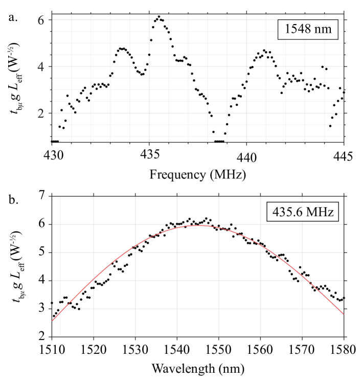
Figure 6: Optical and RF bandwidth The measurements and regression presented in Figure 4 are repeated over a range of wavelengths and RF frequencies to determine the bandwidth of the AOM. a. The RF response is largely determined by how the transucer, specifically $t_{\textrm{b}\mu}$, varies with $\Omega$ and so takes a shape similar to the transducer’s conductance. b. The optical bandwidth is determined by phase-matching. The red curve is the $gt_{\textrm{b}\mu}L_{\textrm{eff}}$ regressed from a simulated dataset with the measured values for $g$, $t_{\textrm{b}\mu}$, and $\gamma$, and $\Delta n_{\textrm{g}}=0.175$.

We repeat the measurements and analysis presented in Figure 4c, varying the RF drive frequency and the optical wavelength away from a phase-matched operating point. The results are plotted in Figure 6. While the RF bandwidth is dictated by the transducer response, the optical bandwidth (Figure 6b) is determined by phase-matching. We simulate a data set from Equation 63 using the measured values for $gt_{\textrm{b}\mu}L_{\textrm{eff}}$ and an optical group index difference $\Delta n_{\textrm{g}}=0.175$. Fits to the simulated data are overlaid (red curve) on the measurements. The best-fit $\Delta n_{\textrm{g}}$ is close to the FEM numerical value of $0.125$.

Appendix C Characterizing the AO Multiplexer

The performance of the multiplexers are summarized in the manuscript. Here we provide details on their characterization.

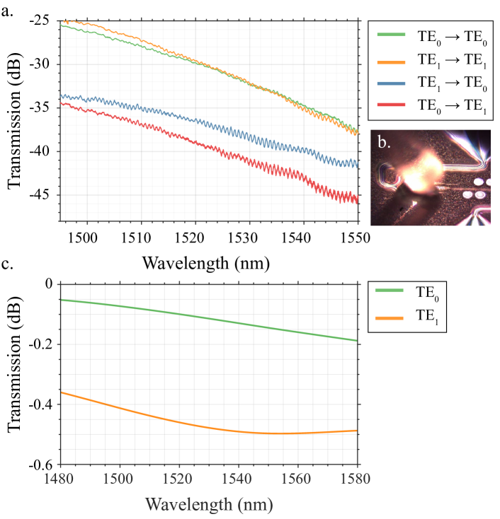
Figure 7: Optics a. FDTD simulations of the insertion loss of both couplers. b. The transmission is measured aligning the fibers to each pair of optical ports. We see -10 dB crosstalk. The center of the grating response is near 1500 nm. c. Photograph of a fiber coupled to the device.

C.1 Optical couplers

The optical couplers are designed to adiabatically transfer the mode of the coupling waveguide into the AO waveguide. Widths of the two waveguides are chosen by solving for the modes of the adjacent waveguides as discussed in Section III in the manuscript. The tapered couplers are simulated by FDTD in Lumerical Lumerical Inc. (2019) and their insertion loss plotted in Figure 7a.

We measure the optical transmission through the device for the four optical paths TE${}_{0/1}\rightarrow$TE_0/1, plotted in Figure 7c. Transmission through the TE₀ and TE₁ paths is similar, both exhibiting $-10~{}$dB crosstalk into the unintended optical mode. This crosstalk limits the isolation of the device. It causes the optical pump to leak through into the signal channel. For example, if light is injected into the TE₁ port (bottom-left in Figure 3), in a perfect device with no crosstalk only photons which absorb a phonon and scatter into the TE₀ mode leave from the bottom-right. With $-10$ dB crosstalk, 10% of the pump remaining at the end of the waveguide is sent into the bottom-right port.

The insertion losses for the different paths through the device are unequal which can arise from, e.g., different efficiencies of the two adiabtic optical couplers or variability in the fab. For example, TE₁$\rightarrow$TE₁ can have a higher insertion loss than TE₁$\rightarrow$TE₀. As a result, if light is fully converted from TE₁ to TE₀ by the mechanics, more light can leave the device with the drive on than with the drive off. The modulation efficiency as defined in Figure 4d and Figure 5b can exceed or not reach 0 dB at the full conversion drive power $P_{\pi/2}$.

C.2 Piezoelectric transducer efficiency and mechanical propagation loss

The design of the transducer and methods for characterizing its efficiency and the mechanical propagation loss are described in detail in References Sarabalis et al. (2020b); Dahmani et al. (2020). The S-matrix of the device in Figure 3 is measured on a calibrated probe station. From the reflection measurements $S_{ii}$ where $i=1$ for the left transducer and $i=2$ for the right, we see that the response of the transducer is repeatable. The reflections (Figure 8a) reach -2 dB for the SH₀ response corresponding to a -4.3 dB loss from impedance mismatch between the $50~{}\Omega$ transmission line and transducer.

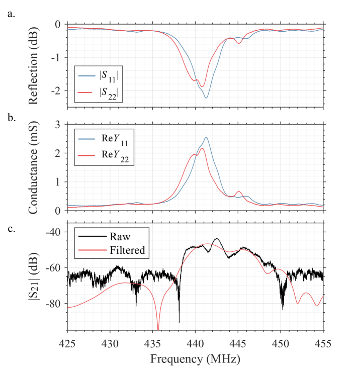
Figure 8: Transducer response The left and right transducer in Figure 3 are ports 1 and 2, respectively. a. The dip in the reflections near 440 MHz corresponds to the SH₀ mode plotted in the bands in Figure 1. b. The conductance reaches 2 mS.c. We overlay the transmission $S_{21}$ filtering out microwave crosstalk and higher-order transits in the device onto the raw data. The filtered response removes ripples from the higher-order transits and is used to extract $t_{\textrm{b}\mu}^{2}e^{-\gamma L/2}$.

The single-port response is not enough to determine the transducer’s efficiency. There are other loss mechanisms in addition to impedance mismatch which reduce the transducer’s efficiency. Of the power emitted into the waveguide, nearly all of it is in the SH₀ mode but, as discussed in detail in Reference Dahmani et al. (2020), resonances in the transducer lead to large material damping losses. In order to determine the transmission coefficient $t_{\textrm{b}\mu}$ from microwaves in the line to phonons in the waveguide, we need to measure the two-port response $S_{21}$ and filter out contributions from triple-transit etc. Sarabalis et al. (2020b). In Figure 8c, we plot the raw $S_{21}$ as well as the single-transit response filtered in the time-domain. This filtered signal is equal to $t_{\textrm{b}\mu}^{2}e^{-\gamma L/2}$, assuming symmetric coefficients for the two transducers. The mechanical losses are independently determined by measuring how the transmission varies with the length of the waveguide $L$. The impulse response $h_{21}$, i.e. the Fourier transform of $S_{21}$, is plotted in Figure 9 where the peaks are fit (inset) for the propagation loss $\gamma$.

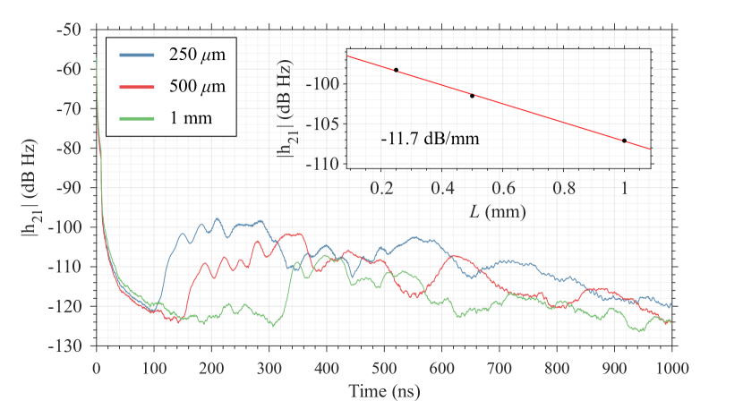
Figure 9: Mechanical propagation loss We extract the propagation loss from a length sweep of the waveguide by fitting a line to the magnitude of the impulse response. We fit an exponential to the peak response yielding $\gamma=-11.7~{}\textrm{dB/mm}$ (inset).

Appendix D RF power-handling

The maximum conversion efficiency observed $\eta_{\textrm{max}}=18\%$ is limited by the microwave power-handling of the transducer and the AO multiplexer. In Figure 10, we plot reflections from the transducer $S_{11}$ measured on a vector network analyzer as the power is increased to $10~{}\textrm{dBm}$ at which $\eta_{\textrm{max}}$ was observed. As the power is increased, the center frequency of the IDT decreases and, for fixed-frequency drives, can cause drops above 1 dB. After removing the 1.2 dB round-trip loss in the cable, this change in $S_{11}$ amounts to a $-3~{}\textrm{dB}$ decrease in the power delivered to the device. This power-dependent frequency shift causes the curves in Figure 4c to deviate from a sinusoid, and so we restrict our fits for $gt_{\textrm{b}\mu}$ to the low-power portion of the dataset.

Not only do we see frequency shifts, at $10~{}\textrm{dBm}$ discontinuities appear in $S_{11}(\Omega)$, evidence of bi-stability arising from, e.g., Duffing nonlinearities.

At 13 dBm drive power, the tethers in the multiplexer broke. The AO and coupling waveguides separated from one another, destroying the optical couplers.

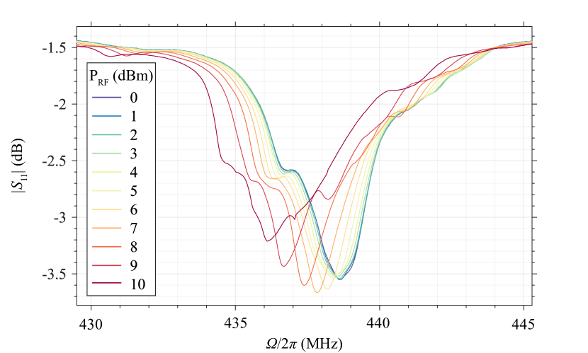
Figure 10: Power-handling of the Transducer Microwave reflections $S_{11}$ form the transducer show a center frequency shift and bi-stabilities as the drive power $P_{\textrm{RF}}$ is increased to $10~{}\textrm{dBm}$.

Appendix E Inferring $g$

In our heterodyne measurements described in Section V, both the pump depletion and converted signal powers are measured, and both can be used to infer $g$. In the low-power limit, the pump depletion provides a better measure of the $P_{\pi/2}$. Given a pump with initial amplitude $a_{0}$, the flux in the pump varies up to $\mathcal{O}\left(\beta^{5}\right)$ as

$$\left|a_{0}\right|^{2}\cos^{2}\left(gt_{\textrm{b}\mu}\beta L\right)\approx\left|a_{0}\right|^{2}\left(1-\left|gt_{\textrm{b}\mu}\beta L\right|^{2}+\frac{1}{3}\left|gt_{\textrm{b}\mu}\beta L\right|^{4}\right).$$ (64)

while the signal power varies as

$$\left|a_{0}\right|^{2}\sin^{2}\left(gt_{\textrm{b}\mu}\beta L\right)\approx\left|a_{0}\right|^{2}\left(\left|gt_{\textrm{b}\mu}\beta L\right|^{2}+\frac{1}{3}\left|gt_{\textrm{b}\mu}\beta L\right|^{4}\right).$$ (65)

Two terms in the series are needed to fit $g\left|t_{\textrm{b}\mu}\right|L$ without independently measuring $\left|a_{0}\right|^{2}$. This is satisfied for the pump to second-order in $\beta$ but to fourth order for the signal, making pump depletion a more sensitive measure of the efficiency in the low-power limit.

The drives used for the dataset in Figure 4 were high enough for independent regressions on the pump and converted signal to give comparable values for $P_{\pi/2}$.

References

- Harris et al. (1970) S. Harris, S. Nieh, and R. Feigelson, Applied Physics Letters 17, 223 (1970).
- Ohmachi and Noda (1977) Y. Ohmachi and J. Noda, IEEE Journal of Quantum Electronics 13, 43 (1977).
- Binh et al. (1980) L. Binh, J. Livingstone, and D. Steven, Optics letters 5, 83 (1980).
- Smith et al. (1990) D. A. Smith, J. E. Baran, J. J. Johnson, and K.-W. Cheung, IEEE journal on selected areas in communications 8, 1151 (1990).
- Hinkov et al. (1994) I. Hinkov, V. Hinkov, and E. Wagner, Electronics Letters 30, 1884 (1994).
- Duchet et al. (1995) C. Duchet, C. Brot, and M. Di Maggio, Electronics Letters 31, 1235 (1995).
- Wang et al. (2014) C. Wang, M. J. Burek, Z. Lin, H. A. Atikian, V. Venkataraman, I.-C. Huang, P. Stark, and M. Lončar, Optics express 22, 30924 (2014).
- Levy et al. (1998) M. Levy, R. Osgood Jr, R. Liu, L. Cross, G. Cargill III, A. Kumar, and H. Bakhru, Applied Physics Letters 73, 2293 (1998).
- Chang et al. (2016) L. Chang, Y. Li, N. Volet, L. Wang, J. Peters, and J. E. Bowers, Optica 3, 531 (2016).
- Rao et al. (2016) A. Rao, M. Malinowski, A. Honardoost, J. R. Talukder, P. Rabiei, P. Delfyett, and S. Fathpour, Optics Express 24, 29941 (2016).
- Yu et al. (2019) M. Yu, C. Wang, M. Zhang, and M. Lončar, IEEE Photonics Technology Letters 31, 1894 (2019).
- Wang et al. (2018) C. Wang, M. Zhang, X. Chen, M. Bertrand, A. Shams-Ansari, S. Chandrasekhar, P. Winzer, and M. Lončar, Nature 562, 101 (2018).
- McKenna et al. (2020) T. P. McKenna, J. D. Witmer, R. N. Patel, W. Jiang, R. Van Laer, P. Arrangoiz-Arriola, E. A. Wollack, J. F. Herrmann, and A. H. Safavi-Naeini, arXiv preprint arXiv:2005.00897 (2020).
- Sarabalis et al. (2020a) C. J. Sarabalis, T. P. McKenna, R. N. Patel, R. Van Laer, and A. H. Safavi-Naeini, APL Photonics 5, 086104 (2020a).
- Olsson III et al. (2014) R. H. Olsson III, K. Hattar, S. J. Homeijer, M. Wiwi, M. Eichenfield, D. W. Branch, M. S. Baker, J. Nguyen, B. Clark, T. Bauer, et al., Sensors and Actuators A: Physical 209, 183 (2014).
- Vidal-Álvarez et al. (2017) G. Vidal-Álvarez, A. Kochhar, and G. Piazza, in 2017 IEEE International Ultrasonics Symposium (IUS) (IEEE, 2017) pp. 1–4.
- Pop et al. (2017) F. V. Pop, A. S. Kochhar, G. Vidal-Alvarez, and G. Piazza, in 2017 IEEE 30th International Conference on Micro Electro Mechanical Systems (MEMS) (IEEE, 2017) pp. 966–969.
- Manzaneque et al. (2019) T. Manzaneque, R. Lu, Y. Yang, and S. Gong, IEEE Transactions on Microwave Theory and Techniques 67, 1379 (2019).
- Sarabalis et al. (2020b) C. J. Sarabalis, Y. D. Dahmani, A. Y. Cleland, and A. H. Safavi-Naeini, Journal of Applied Physics 127, 054501 (2020b).
- Mayor et al. (2020) F. M. Mayor, W. Jiang, C. J. Sarabalis, T. P. McKenna, J. D. Witmer, and A. H. Safavi-Naeini, arXiv preprint arXiv:2007.04961 (2020).
- Dahmani et al. (2020) Y. D. Dahmani, C. J. Sarabalis, W. Jiang, F. M. Mayor, and A. H. Safavi-Naeini, Physical Review Applied 13, 024069 (2020).
- Jiang et al. (2020) W. Jiang, C. J. Sarabalis, Y. D. Dahmani, R. N. Patel, F. M. Mayor, T. P. McKenna, R. Van Laer, and A. H. Safavi-Naeini, Nature communications 11, 1 (2020).
- Brillouin (1922) L. Brillouin, AnPh 9, 88 (1922).
- Wolff et al. (2015) C. Wolff, M. J. Steel, B. J. Eggleton, and C. G. Poulton, Physical Review A 92, 013836 (2015).
- Sipe and Steel (2016) J. Sipe and M. Steel, New Journal of Physics 18, 045004 (2016).
- Van Laer et al. (2016) R. Van Laer, R. Baets, and D. Van Thourhout, Physical Review A 93, 053828 (2016).
- Eggleton et al. (2019) B. J. Eggleton, C. G. Poulton, P. T. Rakich, M. J. Steel, and G. Bahl, Nature Photonics 13, 664 (2019).
- Kittlaus et al. (2017) E. A. Kittlaus, N. T. Otterstrom, and P. T. Rakich, Nature communications 8, 1 (2017).
- Kang et al. (2011) M. S. Kang, A. Butsch, and P. S. J. Russell, Nature Photonics 5, 549 (2011).
- Note (1) If we normalize such that is power instead of flux, the factors of disappears from and throughout the text.
- Dostart and Popović (2020) N. Dostart and M. Popović, arXiv preprint arXiv:2007.11520 (2020).
- Chang et al. (2017) Y.-C. Chang, S. P. Roberts, B. Stern, I. Datta, and M. Lipson, in CLEO: Science and Innovations (Optical Society of America, 2017) pp. SF1J–5.
- Miller (2015) D. A. Miller, Optica 2, 747 (2015).
- Jiang et al. (2019) W. Jiang, R. N. Patel, F. M. Mayor, T. P. McKenna, P. Arrangoiz-Arriola, C. J. Sarabalis, J. D. Witmer, R. Van Laer, and A. H. Safavi-Naeini, Optica 6, 845 (2019).
- Heffner et al. (1988) B. Heffner, D. Smith, J. Baran, A. Yi-Yan, and K. Cheung, Electronics Letters 24, 1562 (1988).
- Frangen et al. (1989) J. Frangen, H. Herrmann, R. Ricken, H. Seibert, W. Sohler, and E. Strake, Electronics Letters 25, 1583 (1989).
- Hinkov and Hinkov (1991) I. Hinkov and V. Hinkov, Electronics Letters 27, 1211 (1991).
- Hinkov et al. (1988) V. Hinkov, R. Opitz, and W. Sohler, Journal of lightwave technology 6, 903 (1988).
- Liu et al. (2019) Q. Liu, H. Li, and M. Li, Optica 6, 778 (2019).
- Kittlaus et al. (2020) E. A. Kittlaus, W. M. Jones, P. T. Rakich, N. T. Otterstrom, R. E. Muller, and M. Rais-Zadeh, arXiv preprint arXiv:2004.01270 (2020).
- Smith (1973) R. Smith, IEEE Journal of Quantum Electronics 9, 545 (1973).
- Tien et al. (2011) M.-C. Tien, T. Mizumoto, P. Pintus, H. Kromer, and J. E. Bowers, Optics express 19, 11740 (2011).
- Ghosh et al. (2012) S. Ghosh, S. Keyvavinia, W. Van Roy, T. Mizumoto, G. Roelkens, and R. Baets, Optics Express 20, 1839 (2012).
- Heeks and Jackson (1986) J. S. Heeks and J. D. Jackson, “Acousto-optic isolator,” (1986), uS Patent 4,606,614.
- O’meara (1988) T. R. O’meara, “Acousto-optical laser isolator,” (1988), uS Patent 4,736,382.
- Li et al. (2014) E. Li, B. J. Eggleton, K. Fang, and S. Fan, Nature communications 5, 1 (2014).
- Peano et al. (2015) V. Peano, C. Brendel, M. Schmidt, and F. Marquardt, Physical Review X 5, 031011 (2015).
- Sohn et al. (2018) D. B. Sohn, S. Kim, and G. Bahl, Nature Photonics 12, 91 (2018).
- Sarabalis et al. (2018) C. J. Sarabalis, R. Van Laer, and A. H. Safavi-Naeini, Optics Express 26, 22075 (2018).
- Sohn and Bahl (2019) D. B. Sohn and G. Bahl, APL Photonics 4, 126103 (2019).
- Williamson et al. (2020) I. A. Williamson, M. Minkov, A. Dutt, J. Wang, A. Y. Song, and S. Fan, arXiv preprint arXiv:2002.04754 (2020).
- Fu et al. (2019) W. Fu, Z. Shen, Y. Xu, C.-L. Zou, R. Cheng, X. Han, and H. X. Tang, Nature communications 10, 1 (2019).
- Yariv (1973) A. Yariv, IEEE Journal of Quantum Electronics 9, 919 (1973).
- Johnson et al. (2002) S. G. Johnson, M. Ibanescu, M. Skorobogatiy, O. Weisberg, J. Joannopoulos, and Y. Fink, Physical review E 65, 066611 (2002).
- Andrushchak et al. (2009) A. Andrushchak, B. Mytsyk, H. Laba, O. Yurkevych, I. Solskii, A. Kityk, and B. Sahraoui, Journal of Applied Physics 106, 073510 (2009).
- Snyder and Love (2012) A. W. Snyder and J. Love, Optical waveguide theory (Springer Science & Business Media, 2012).
- Auld (1973) B. A. Auld, Acoustic fields and waves in solids, Vol. II (John Wiley & Sons, 1973).
- Lumerical Inc. (2019) Lumerical Inc., “FDTD: 3d electromagnetic simulator,” (2019).