CLOUD: Contrastive Learning of Unsupervised Dynamics

Abstract

Developing agents that can perform complex control tasks from high dimensional observations such as pixels is challenging due to difficulties in learning dynamics efficiently. In this work, we propose to learn forward and inverse dynamics in a fully unsupervised manner via contrastive estimation. Specifically, we train a forward dynamics model and an inverse dynamics model in the feature space of states and actions with data collected from random exploration. Unlike most existing deterministic models, our energy-based model takes into account the stochastic nature of agent-environment interactions. We demonstrate the efficacy of our approach across a variety of tasks including goal-directed planning and imitation from observations. Project videos and code are at https://jianrenw.github.io/cloud/.

Keywords: Self-supervised, Learning Dynamics, Model-based Control, Visual Imitation

1 Introduction

Modeling dynamics in the physical world is an essential and fundamental problem in the robotics applications, such as manipulation [1, 2], planning [3, 4, 5], and model-based reinforcement learning [6, 7]. To perform complex control tasks in an unknown environment, an agent needs to learn the dynamics from experience [8, 9, 10]. However, developing agents that can learn dynamics directly from high dimensional observations such as pixels is known to be challenging [11, 7, 12].

There are three key challenges. First, learning informative representations of the states from raw images is difficult. Second, the dynamics of real-world objects are always complex and nonlinear, especially for deformable objects. Third, modeling the stochasticity of the agent-environment system is extremely challenging. The stochasticity mainly comes from two aspects: the noise in the agent’s actuation and the inherent uncertainty in the environment, both of which cannot be ignored. Many recent works have been proposed to tackle these challenges. A direct approach is to learn complex dynamics models from the pixel space [13, 14]. Kurutach et al. [3] suggested learning a generative model of sequential observations, where the generative process is induced by a transition in a low-dimensional planning model, and additional noise. Their work can model the stochastic transition function. However, making predictions in raw sensory space is not only hard but is also irrelevant to the agent’s goals, e.g. a model needs to capture appearance changes in order to make photo-realistic predictions, which makes it hard to generalize across physically similar but visually distinct environments. One possible solution is to predict those changes in the space that affect or be affected by the agent, and ignore rest of the unrelated dynamics. For example, instead of making predictions in the pixel space, we could transform the sensory input into a feature space where only the information relevant to the agent actions are represented. Agrawal et al. [9] proposed to jointly train forward and inverse dynamics models, where a forward model predicts the next state from the current state and action, and an inverse model predicts the action given the initial and target states. In the joint training, the inverse model objective provides supervision for transforming image pixels into an abstract feature space, while the forward model can predict in it. The inverse model alleviates the need for the forward model to make predictions in the raw pixel space, and the forward model in turn regularizes the feature space for the inverse model. This simple strategy has been adopted by many works [8, 15]. However, these methods can hardly learn predictive models beyond noise-free environments. Despite several methods to build stochastic models in low-dimensional state space [16, 17], scaling it to high dimensional inputs (e.g., images) still remains challenging.

In this paper, we introduce a novel method, named CLOUD, that uses contrastive learning [18] to handle all the above challenges. Inspired by [9], we jointly train a forward dynamics model, an inverse dynamics model, a state representation model, and an action representation model with contrastive objectives. The forward dynamics model is trained to maximize the agreement between the predicted and the observed next state representations; the inverse dynamics model is trained to maximize the agreement between the predicted and the ground truth action representations. Our proposed approach offers three unique advantages. First, contrastive learning only measures the compatibility between prediction and observation, which can handle the stochasticity by nature [19]. Second, by introducing an action representation, our method can generalize over large, finite action sets by allowing the agent to infer the outcomes of actions similar to actions previously taken [20]. Third, building upon SimCLR [18], our proposed method is data-efficient and can be trained in a fully unsupervised manner.

To summarize, 1) we propose a general framework to learn a forward dynamics model, an inverse dynamics model, a state representation model, and an action representation model jointly; 2) using contrastive estimation, our proposed method can handle the stochasticity of the agent-environment system naturally; 3) we demonstrate the efficacy of our approach across a variety of tasks including goal-directed planning and imitation from observations.

2 Related Works

Contrastive Learning

Contrastive Learning is a framework to learn representations that obey similarity constraints in a dataset typically organized by similar and dissimilar pairs. There has been a large number of prior works. Hadsell et al. [21] first propose to learn representations by contrasting positive pairs against negative pairs. Wu et al. [22] propose to use a memory bank to store the instance class representation vector, which is adopted and extended by several recent papers [23, 24]. Other work explores the use of in-batch samples for negative sampling instead of a memory bank [25, 23, 26]. Recently, SimCLR [18] and MoCo [27, 28] achieved state-of-the-art results in self-supervised visual representations learning, bridging the gap with supervised learning.

Learning Dynamics

Modelling dynamics is a long-standing problem in both robotics and artificial intelligence. One line of work is to estimate physical properties directly from their appearance and motion, which is known as intuitive physics [29, 30, 31, 32, 33, 34]. These models build upon an explicit physical model, i.e., a model parameterized by physical properties such as mass and force. This enables generalization to new scenarios, but also limits their practical usage: annotations on physical parameters in real-world applications are expensive and challenging to obtain. An alternative line of work is to learn object representations without explicit modeling of physical properties, but in a self-supervised way through robot interactions. Byravan et al. [35] propose to use deep networks to approximate rigid object motion. Agrawal et al. [9] suggest encoding physical properties in latent representations that can be decoded through forward and inverse dynamics models. A few follow-ups have extended these models for rope manipulation [8], pushing via transfer learning [36], and planning [3, 4]. A concurrent work from Yan etal. [37] has also demonstrated the effectiveness of using contrastive estimation to learn predictive representations. Different from them, we focus on forward and backward dynamics reasoning under stochastic environment.

Imitation from Observations

Increasingly, works have aspired to learn from observation alone without utilizing expert actions [38]. e.g., Liu et al. [39] propose to learn to imitate from videos without actions and translates from one context to another. Ho et al. [40] propose to learn features for a reward signal that is later used for reinforcement learning. Few recent works aim to learn inverse dynamics in a self-supervised manner, then given a task, attempt it zero-shot [5, 41, 38].

3 Method

Our framework consists of four learnable functions, including a forward dynamics model $F(\cdot)$, an inverse dynamics model $I(\cdot)$, a state representation model $g(\cdot)$ and an action representation model $q(\cdot)$. We propose to learn these four models jointly via contrastive estimation. We begin by discussing the state representation model and action representation model. Following that, we discuss the forward dynamics model and inverse dynamic model. Finally, we discuss how to use contrastive estimation to jointly optimize these four models in an unsupervised manner. The notation is as following: $s_{t},a_{t}$ are the world state and action applied time step $t$, $s_{t+1}$ is the world state at time step $t+1$. $E$ represents the stochastic environment, where $s_{t+1}$ can be sampled from $s_{t+1}\sim E(s_{t},a_{t})$. See Figure 1 for an illustration of the formulation.

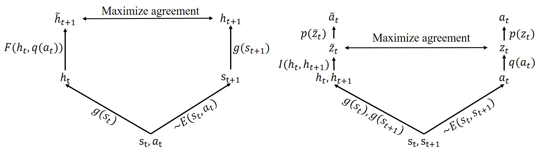
Figure 1: CLOUD Architecture: Our framework consists of four learnable functions, including a forward dynamics model $F(\cdot)$, an inverse dynamics model $I(\cdot)$, a state representation model $g(\cdot)$ and an action representation model $q(\cdot)$. We propose to learn these four models jointly via contrastive estimation.

3.1 State and Action Representation Models

The benefits of capturing the structure in the underlying state space is a well understood and widely used concept in robotics. Given a set of states $\{s\}\subseteq\mathcal{S}$ (where the states are raw sensory inputs), the goal of state representation model $g(\cdot)$ is to encode high-dimensional images $s$ into informative representations $h$, which is mathematically described as $h=g(s)$. State representations allow the policy to generalize across states. Ideally, the value comparisons between these features should correlate well with true distances between these states. Naturally, such features would be useful later for planning.

Similarly, there often exists additional structure in the space of actions that can be leveraged. Given a set of actions $\{a\}\subseteq\mathcal{A}$, we introduce an action representation model $q(\cdot)$ to encode actions $a$ into embeddings $z$, which is mathematically described as $z=q(a)$. We then propose to use an action decoder $p(\cdot)$ that deterministically maps this representation to the action, which is denoted as $a=p(z)$.

3.2 Forward and Inverse Dynamics Models

Forward dynamics models and inverse dynamics models have been studied for a long time. Let $\{(s_{t},a_{t},s_{t+1})\}$ represent a set of state-action-state tuples. A model that predicts the state of the next timestep $\tilde{s}_{t+1}$ given current state and action $s_{t},a_{t}$ is known as a forward dynamics model $F(\cdot)$, and is mathematically described as $\tilde{s}_{t+1}=F(s_{t},a_{t})$. Instead of directly learning a dynamics model through pixel space, we consider to make predictions in a learned latent space. Because making predictions in raw sensory space is hard and can always be distracted by irrelevant information [3]. Thus, our forward dynamics model can be mathematically described in Equation 1 below:

$$\tilde{h}_{t+1}=F(h_{t},z_{t}),$$ (1)

where $h_{t}=g(s_{t}),z_{t}=q(a_{t})$.

Oe other hand, a model that predicts the action $a_{t}$ that relates a pair of input states $(s_{t},s_{t+1})$ is called an inverse dynamics model $I(\cdot)$. Similarly, we consider to make predictions in a learned action space, which is described as following:

$$\tilde{z}_{t}=I(h_{t},h_{t+1}),$$ (2)

where $h_{t}=g(s_{t}),h_{t+1}=g(s_{t+1})$.

3.3 Contrastive Estimation

Many works [8, 9, 5] directly optimize the above mentioned models by forcing $h_{t+1}=\tilde{h}_{t+1}$ and $z_{t}=\tilde{z}_{t}$. However, by forcing predicted representations equal to observed future representations, these methods also assume the transition to be deterministic, which is always not true in the real world. The real environment is always stochastic (e.g. coin toss), where deterministic functions can only predict the average.

On the other hand, contrastive estimation is an energy-based model. Instead of setting the cost function to be zero only when the prediction and the observation are the same, energy-based model assigns low cost to all compatible prediction-observation pairs. Thus, constrastive estimation can handle the stochasticity by its nature [19]. Inspired by recent contrastive learning algorithms [18], we propose to train these models by maximizing agreement between predicted and real representations via a contrastive loss. We randomly sample a minibatch of N state-action-state tuples $\{(s^{i}_{t},a^{i}_{t},s^{i}_{t+1})\}$. For forward dynamics model, a prediction $\tilde{h}^{i}_{t+1}$ and real representation $h^{i}_{t+1}$ from the same tuple is defined as positive example. Following SimCLR [18], we treat the other $2(N-1)$ real representation $(h^{j}_{t},h^{j}_{t+1})|j\neq i$ within a minibatch as negative examples. We use cosine similarity to denote the distance between two representation $(u,v)$, that is $\texttt{sim}(u,v)=\mathbf{u}^{T}\cdot\mathbf{v}/||\mathbf{u}||\cdot||\mathbf{v}||$. The loss function for a positive pair of examples $(\tilde{h}^{i}_{t+1},h^{i}_{t+1})$ is defined as:

$$l_{F}=-\text{log}\frac{\text{exp}(\texttt{sim}(\tilde{h}^{i}_{t+1},h^{i}_{t+1})/\tau)}{\sum_{\begin{subarray}{c}j=1\\ j\neq i\end{subarray}}^{N}\text{exp}(\texttt{sim}(\tilde{h}^{i}_{t+1},h^{j}_{t})/\tau)+\sum_{\begin{subarray}{c}j=1\\ j\neq i\end{subarray}}^{N}\text{exp}(\texttt{sim}(\tilde{h}^{i}_{t+1},h^{j}_{t+1})/\tau)},$$ (3)

where $\tau$ denotes a temperature parameter that is empirically chosen as $0.1$.

Similarly, for inverse dynamics model, the loss function for a positive pair of examples $(\tilde{z}^{i}_{t},z^{i}_{t})$ is defined as:

$$l_{I}=-\text{log}\frac{\text{exp}(\texttt{sim}(\tilde{z}^{i}_{t},z^{i}_{t})/\tau)}{\sum_{\begin{subarray}{c}j=1\\ j\neq i\end{subarray}}^{N}\text{exp}(\texttt{sim}(\tilde{z}^{i}_{t},z^{j}_{t})/\tau)+\sum_{\begin{subarray}{c}j=1\\ j\neq i\end{subarray}}^{N}\text{exp}(\texttt{sim}(\tilde{z}^{i}_{t},z^{j}_{t+1})/\tau)}.$$ (4)

During joint training, the total loss is computed across all positive pairs in a mini-batch.

4 Experiments

We evaluate our proposed method in comparison with classical baseline methods on two tasks, goal-directed planning and imitation from observations on rope manipulation. The details of the datasets and other experimental settings are described below.

4.1 Representation Visualization

To understand the representation models, we first propose to visualize the state representations learned by our model using t-SNE [42]. With t-SNE visualizations there tends to be many overlapping points in the 2D space, which increases the difficulty of viewing overlapped state examples. Therefore, we quantize t-SNE points into a 2D grid with $40\times 20$ interface, using RasterFairy [43].

In Figure 2, we show the state representations from validation set which are not seen during training. Notice that similar configurations of the rope appear near each other, indicating the learned feature space meaningfully organizes variation in rope shape.

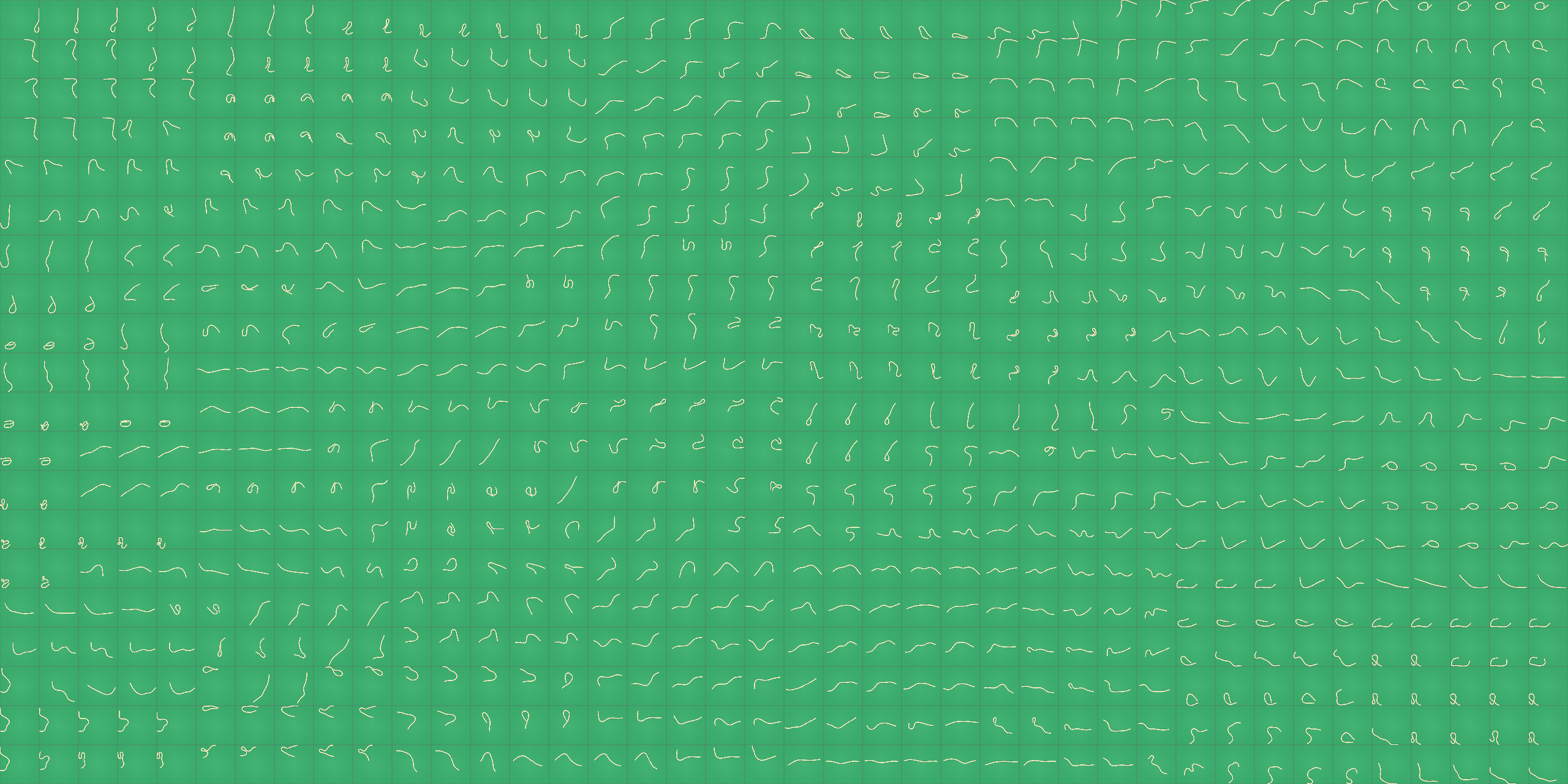
Figure 2: t-SNE Visualization of State Representation. The grid interface is $40\times 20$, fit with image examples from validation set.

4.2 Goal-Directed Planning

In goal-directed planning, an agent is required to generate a plausible sequence of states that transition a dynamical system from its current configuration to the desired goal state. Given the learned representations and dynamics models, we propose to plan with a simple version of goal-directed planning (MPC). We first sample several actions and then feed them to the forward dynamics model. Finally, we choose the action that leads to the largest cosine similarity between predicted state representation and goal state representation. The procedure is repeated iteratively for 20 steps.

Dataset and Settings.

To simulate rope, we use the DeepMind Control Suite [44] with MuJoCo physics engine [45]. The rope is represented by 25 geoms in simulation with a four-dimensional action space $(x_{1},y_{1},x_{2},y_{2})$: the first two dimensions $(x_{1},y_{1})$ denote the pick point on the rope, and the last two dimensions $(x_{2},y_{2})$ are the drop location, both of which are in the pixel coordinates of the input RGB image. In order to evaluate the performance of CLOUD under a stochastic environment, we add Gaussian noise to each geom after actions are executed. We use an overhead camera that renders RGB images as input observations for training our model.

By randomly perturbing the rope, our data is collected in a completely unsupervised manner. The interaction of the agent with rope is uniformly sampled but constrained to the observed field to avoid redundant data. We collect 10k trajectories of length 20 (200k samples), which are further split into 150k training samples and 50k testing samples.

We evaluate the performance of goal-directed planning on two types of goal states: shaped and straight. Following [9], we manually pick a set of complex rope shapes for an agent to reach, including ”C”, ”L”, ”S” and ”knot”, which are denoted as ”shaped goal state”. For straight goal state, the agent is supposed to straighten the rope from a given initial configuration.

The performance is quantitatively measured by calculating Euclidean distance between two sets of geoms from achieved and goal states correspondingly, which attempt to capture the deviation between desired goals and agent achieved final states. A successful manipulation is judged by whether the mean distance error is below the threshold (set according to human observation, we use 4 of each geom in pixel space) at each run to calculate the success rate.

Training Details.

For state representation model $g(\cdot)$, we use a series of 2D convolutions to extract useful features from $64\times 64$ raw RGB images. The output is then flattened and fed into a linear layer to produce low-dimensional embeddings of the state representations $h$ in $\mathbf{R^{16}}$. For action representation model $g(\cdot)$, we use a 4-layer MLP to extract useful features from actions and output 16-dimension action embeddings. The forward model is a 4-layer MLP which takes a state representation, and an action representation as input and then outputs the representation of the next state. The inverse model is a 4-layer MLP which takes two state representations as input and then outputs the corresponding action representation.

We use the Adam optimizer [46] for training the network with a batch size of 128 and a learning rate of 1e-3 with a weight decay of 1e-6. We train the network for 30 epochs and report the average success rate for evaluation.

Results.

Table 1 shows the success rate for various approaches for goal-directed planning. We evaluate two different variants of our method:

• CLOUD (F): This method refers to a variant of CLOUD without the inverse dynamics model, where we feed raw actions instead of action embeddings to the forward dynamics model. The purpose of this variant is to particularly ablate the benefit of our inverse dynamics model.

• CLOUD (FI): Our complete model composes of all the four components, including a forward dynamics component, an inverse dynamics component, a state representation component and an action representation component. These components are trained jointly via contrastive estimation in an unsupervised manner.

We compare our results to the following baselines:

• Auto-encoder: We train a simple autoencoder to minimize the pixel distance between reconstructed and actual images [47]. The latent embedding is then used for MPC during planning.

• PlaNet: We train PlaNet [48], a purely model-based agent that learns the dynamics from interactions with the world. Their method predicts actions by fast online planning in latent space through images.

• Predictive Model: We train a predictive model as proposed by Agrawal et al. [9] that jointly learns a forward and inverse dynamics model for intuitive physics. The latent embedding is then used for MPC during planning.

Goal-directed planning (Success %)
Method	Deterministic environment		Stochastic environment
	shaped	straight	shaped	straight
Auto-encoder	$32.8\%\pm{3.9\%}$	$50.9\%\pm{2.9\%}$	$16.5\%\pm{9.9\%}$	$42.1\%\pm{7.5\%}$
PlaNet	$29.8\%\pm{3.7\%}$	$53.7\%\pm{3.2\%}$	$19.9\%\pm{5.4\%}$	$45.2\%\pm{6.1\%}$
Predictive Model	$34.8\%\pm{2.2\%}$	$53.3\%\pm{0.7\%}$	$18.5\%\pm{9.2\%}$	$40.9\%\pm{7.3\%}$
CLOUD (F)	$43.3\%\pm{1.5\%}$	$53.4\%\pm{0.7\%}$	$41.6\%\pm{2.3\%}$	$\bm{54.6\%}\pm{\bm{1.2\%}}$
CLOUD (FI)	$\bm{49.9}\%\pm{\bm{1.4\%}}$	$\bm{60.8\%}\pm{\bm{1.7\%}}$	$\bm{43.2}\%\pm{\bm{1.5\%}}$	$53.1\%\pm{6.7\%}$

Table 1: Success rate on the goal-directed planning task. Our method outperforms all baseline methods. Prominently, it gets a negligible decline in performance in the stochastic environment, indicating that learning dynamics via contrastive estimation performs better and more robustly than deterministic models.

Results show that our method consistently outperforms all baselines in both shaped goal state and straight goal state. As can be seen in Table 1, when the goal state is simpler, all approaches achieve better performance. We also show that training jointly with an inverse dynamics component instead of a single forward dynamics model performs better on rope manipulation. Such a jointly training strategy regularizes the state and action representation to extract useful information for planning. The poor performance of Auto-encoder also proves the importance of jointly optimizing forward and inverse dynamics models.

Importantly, our method gets a relatively negligible decline in the success rate compared with all baselines under a stochastic environment. The most likely reason is that contrastive estimation assigns a low cost to all possible predictions instead of predicting the average future, given the fact that our method adopts the same architecture as the Predictive Model. Similarly, PlaNet uses a variational encoder, which leads to better performance under a stochastic environment.

We also show qualitative results of various approaches manipulating the rope under a stochastic environment in Figure 3. Each trajectory runs for 20 actions with the same start state and goal state. In the task of manipulating the rope into a ”knot” shape, with our method, the agent successfully achieves the goal state. In comparison, all other methods fail to reach the goal state.

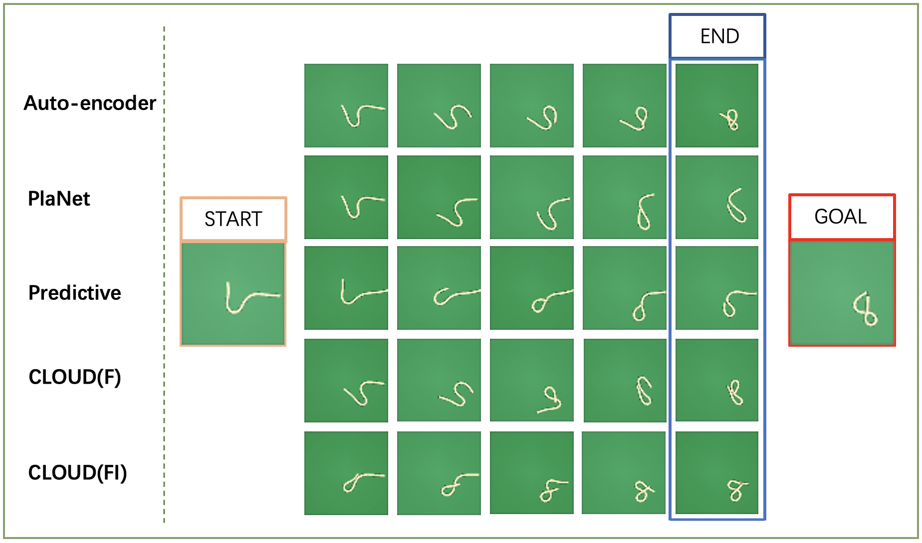
Figure 3: Trajectories of different models on the goal-directed planning task. All agents start from the same start state and are asked to reach the same goal state. Each trajectory is run for 20 actions. Note that the end states of our method achieves the highest similarity with goal state compare with all other methods.

4.3 Imitation from Observations

The goal of imitation from observation is to have the robot watch a sequence of images depicting each stage of the demonstration and then reproduce this demonstration on its own. We adopt the imitation method from Nair et al. [8]. The robot receives a demonstration in the form of a sequence of images of the rope in intermediate states toward a final goal. We denote this sequence of demonstration as $\mathcal{D}=(d_{0},d_{1},...,d_{T})$, where $T$ is the length of demonstration. Let $s_{1}$ be the initial visual state of the robot and $d_{i}$ be the goal visual state. The robot first inputs the pair of states $(s_{1},d_{2})$ into the learned inverse dynamics model and executes the predicted action. Let $s_{2}$ be the visual state of the world after the action is executed. The robot then inputs $(s_{2},d_{3})$ into the inverse model and executes the output action. This process is repeated iteratively for $T$ time steps.

Dataset and Settings.

We use the same environment, dataset and metric as mentioned in Section 4.2 to quantitatively evaluate the performance of imitation from observations. In this task, the trajectory through which the agent achieves the final state is important. Therefore, we consider the average distance of the entire trajectory instead of only using final states when calculating the success rate (mean distance error threshold is set to 4 pixels of each geom).

Training Details.

We use the same network architecture and training procedure as mentioned in Section 4.2. We further use a 4-layer MLP to decode action representations back to actual actions during execution.

Results.

Table 2 shows the success rate of various approaches on imitation from observations. We evaluate two different versions of our method:

• CLOUD (I): The method refers to a variant of CLOUD without using the forward dynamics model. The purpose of this variant is to particularly ablate the benefit of our forward dynamics model.

• CLOUD (FI): In contrast to CLOUD (I), it refers to our complete model. During inference, we utilize its inverse dynamics component for imitation from observation.

We compare our results with the following baselines:

• Nearest Neighbor baseline: To evaluate whether the neural network simply memorizes the training data, we implement a nearest neighbor baseline. Given a pair of states $(s_{t},d_{t+1})$, we find the state transition in the training set that is closest to $(s_{t},d_{t+1})$. The action is then executed. We use Euclidean distance in the pixel space as the distance metric.

• Self-supervised Imitation: We also compare our method with self-supervised imitation proposed by Nair et al. [8]. We reimplement this baseline and train in our setup for a fair comparison.

Imitation from observations (Success %)
Method	Deterministic environment		Stochastic environment
	shaped	straight	shaped	straight
Nearest Neighbor	$17.5\%\pm{4.7\%}$	$19.3\%\pm{3.8\%}$	$10.7\%\pm{3.6\%}$	$16.7\%\pm{5.1\%}$
Self-supervised Imitation	$20.6\%\pm{5.8\%}$	$25.5\%\pm{2.4\%}$	$12.3\%\pm{4.6\%}$	$19.1\%\pm{2.9\%}$
CLOUD (I)	$30.7\%\pm{4.5\%}$	$\bm{56.8}\%\pm{\bm{3.9\%}}$	$26.8\%\pm{3.7\%}$	$48.1\%\pm{5.7\%}$
CLOUD (FI)	$\bm{36.7}\%\pm{\bm{2.8\%}}$	$54.9\%\pm{2.3}$	$\bm{32.4\%}\pm{\bm{3.1\%}}$	$\bm{49.9\%}\pm{\bm{1.9\%}}$

Table 2: Success rate of imitation from observations. The performance of our method is better than baseline methods both in straightening rope and manipulating rope in desired shapes. The gap between stochastic environment and deterministic environment shrinks via contrastive learning.

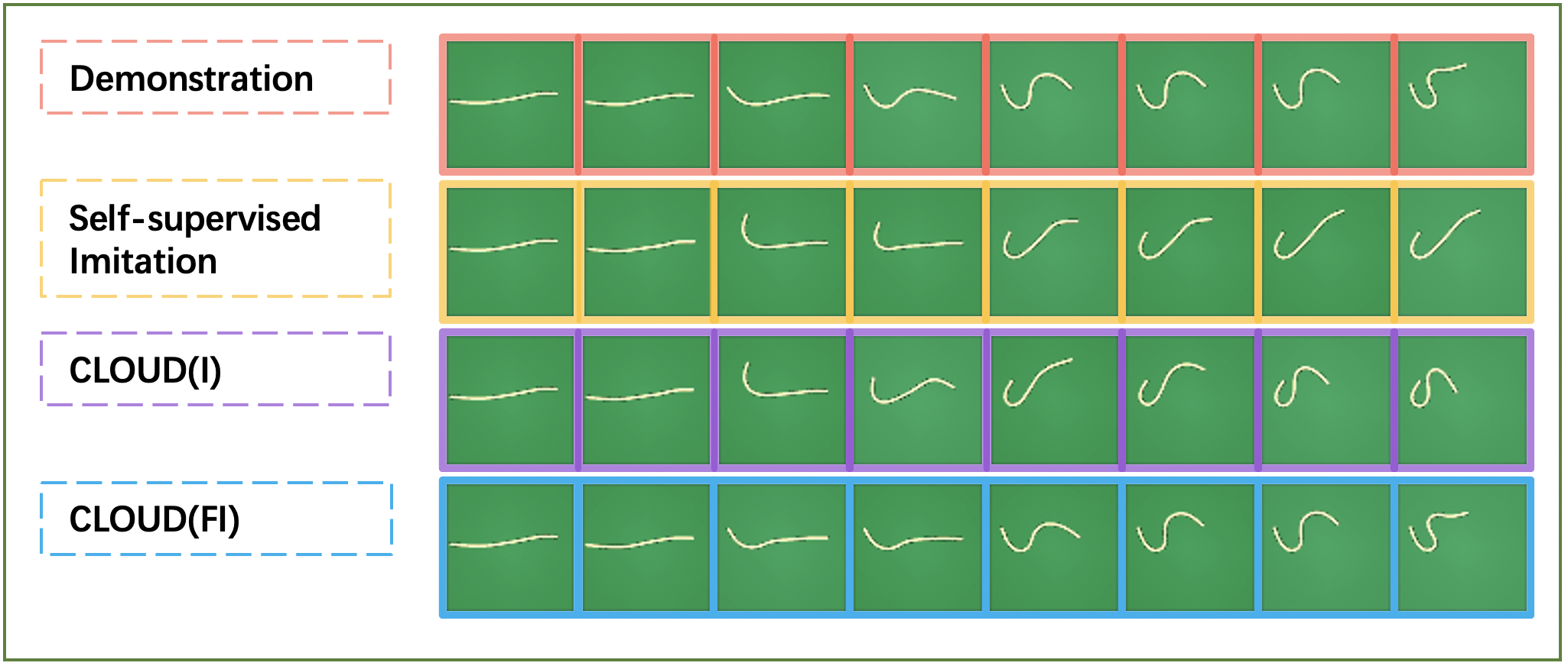
Figure 4: Trajectories of imitation from observations. The upper row represents an example expert demonstration. The following rows show the states achieve by the agent during imitation. The trajectory generated by our method achieves the highest similarity with the demonstration.

Results show that our method outperforms all baselines methods for imitation from observations under both shaped and straight goal states. It worth noticing that Self-supervised Imitation performs similarly with Nearest Neighbor baseline, especially under a stochastic environment, which suggests that deterministic prediction somehow memorize the training data and fail to generalize to the stochastic environments. On the contrary, our methods perform much better than the baseline methods, which further proves the importance of contrastive estimation.

Comparing CLOUD (I) with CLOUD (FI), we show that the state and action representation model can benefit from jointly optimizing forward and inverse dynamics model. The reason is the joint dynamics model regularizes state and action representations to only the information relevant to dynamics. By limiting the dimension of these representations, irrelevant information (e.g. background color, lighting) can be filtered automatically, which leads to better generalization.

Figure 4 qualitatively shows that our method is capable of imitating given demonstrations. We see that our method more accurately re-configure the rope to imitate the demonstration comparing with baseline methods.

5 Conclusion

In conclusion, we proposed CLOUD, a contrastive estimation framework for unsupervised dynamics learning. We show that our learned dynamics are effective for both goal conditioned planning and imitation from observations. Although we only evaluate our method on rope manipulation, there are no task specific assumptions. In future work, we plan to extend CLOUD on more robotic tasks under more complex environments. We hope our work points a new way to learn plannable representations, dynamics models that can handle stochasticity of the environment.

Acknowledgments

If a paper is accepted, the final camera-ready version will (and probably should) include acknowledgments. All acknowledgments go at the end of the paper, including thanks to reviewers who gave useful comments, to colleagues who contributed to the ideas, and to funding agencies and corporate sponsors that provided financial support.

References

- De Schutter and Van Brussel [1988] J. De Schutter and H. Van Brussel. Compliant robot motion i. a formalism for specifying compliant motion tasks. IJRS, 7(4):3–17, 1988.
- Karayiannidis et al. [2016] Y. Karayiannidis, C. Smith, F. E. V. Barrientos, P. Ögren, and D. Kragic. An adaptive control approach for opening doors and drawers under uncertainties. IEEE Transactions on Robotics, 32(1):161–175, 2016.
- Kurutach et al. [2018] T. Kurutach, A. Tamar, G. Yang, S. J. Russell, and P. Abbeel. Learning plannable representations with causal infogan. In NeurIPS, pages 8733–8744, 2018.
- Hafner et al. [2019] D. Hafner, T. Lillicrap, I. Fischer, R. Villegas, D. Ha, H. Lee, and J. Davidson. Learning latent dynamics for planning from pixels. In ICML, pages 2555–2565, 2019.
- Pathak et al. [2018] D. Pathak, P. Mahmoudieh, G. Luo, P. Agrawal, D. Chen, Y. Shentu, E. Shelhamer, J. Malik, A. A. Efros, and T. Darrell. Zero-shot visual imitation. In ICLR, 2018.
- Nagabandi et al. [2018] A. Nagabandi, G. Kahn, R. S. Fearing, and S. Levine. Neural network dynamics for model-based deep reinforcement learning with model-free fine-tuning. In ICRA, pages 7559–7566, 2018.
- Kaiser et al. [2019] Ł. Kaiser, M. Babaeizadeh, P. Miłos, B. Osiński, R. H. Campbell, K. Czechowski, D. Erhan, C. Finn, P. Kozakowski, S. Levine, et al. Model based reinforcement learning for atari. In ICLR, 2019.
- Nair et al. [2017] A. Nair, D. Chen, P. Agrawal, P. Isola, P. Abbeel, J. Malik, and S. Levine. Combining self-supervised learning and imitation for vision-based rope manipulation. In ICRA, pages 2146–2153. IEEE, 2017.
- Agrawal et al. [2016] P. Agrawal, A. V. Nair, P. Abbeel, J. Malik, and S. Levine. Learning to poke by poking: Experiential learning of intuitive physics. In NeurIPS, pages 5074–5082, 2016.
- Kumar et al. [2016] V. Kumar, E. Todorov, and S. Levine. Optimal control with learned local models: Application to dexterous manipulation. In ICRA, pages 378–383. IEEE, 2016.
- Lake et al. [2017] B. M. Lake, T. D. Ullman, J. B. Tenenbaum, and S. J. Gershman. Building machines that learn and think like people. Behavioral and brain sciences, 40, 2017.
- Laskin et al. [2020] M. Laskin, A. Srinivas, and P. Abbeel. Curl: Contrastive unsupervised representations for reinforcement learning. ICML, 2020.
- Chen et al. [2016] X. Chen, Y. Duan, R. Houthooft, J. Schulman, I. Sutskever, and P. Abbeel. Infogan: Interpretable representation learning by information maximizing generative adversarial nets. In NeurIPS, pages 2172–2180, 2016.
- Ebert et al. [2018] F. Ebert, C. Finn, S. Dasari, A. Xie, A. Lee, and S. Levine. Visual foresight: Model-based deep reinforcement learning for vision-based robotic control. arXiv preprint arXiv:1812.00568, 2018.
- Pathak et al. [2017] D. Pathak, P. Agrawal, A. A. Efros, and T. Darrell. Curiosity-driven exploration by self-supervised prediction. In ICML, pages 2778–2787, 2017.
- Chua et al. [2018] K. Chua, R. Calandra, R. McAllister, and S. Levine. Deep reinforcement learning in a handful of trials using probabilistic dynamics models. In NeurIPS, pages 4754–4765, 2018.
- Houthooft et al. [2016] R. Houthooft, X. Chen, Y. Duan, J. Schulman, F. De Turck, and P. Abbeel. Vime: Variational information maximizing exploration. In NeurIPS, pages 1109–1117, 2016.
- Chen et al. [2020] T. Chen, S. Kornblith, M. Norouzi, and G. Hinton. A simple framework for contrastive learning of visual representations. arXiv preprint arXiv:2002.05709, 2020.
- LeCun et al. [2006] Y. LeCun, S. Chopra, R. Hadsell, M. Ranzato, and F. Huang. A tutorial on energy-based learning. Predicting structured data, 1(0), 2006.
- Chandak et al. [2019] Y. Chandak, G. Theocharous, J. Kostas, S. Jordan, and P. Thomas. Learning action representations for reinforcement learning. In ICML, pages 941–950, 2019.
- Hadsell et al. [2006] R. Hadsell, S. Chopra, and Y. LeCun. Dimensionality reduction by learning an invariant mapping. In CVPR, volume 2, pages 1735–1742. IEEE, 2006.
- Wu et al. [2018] Z. Wu, Y. Xiong, S. X. Yu, and D. Lin. Unsupervised feature learning via non-parametric instance discrimination. In CVPR, pages 3733–3742, 2018.
- Ye et al. [2019] M. Ye, X. Zhang, P. C. Yuen, and S.-F. Chang. Unsupervised embedding learning via invariant and spreading instance feature. In CVPR, pages 6210–6219, 2019.
- Tian et al. [2019] Y. Tian, D. Krishnan, and P. Isola. Contrastive multiview coding. arXiv preprint arXiv:1906.05849, 2019.
- Doersch and Zisserman [2017] C. Doersch and A. Zisserman. Multi-task self-supervised visual learning. In ICCV, 2017.
- Ji et al. [2019] X. Ji, J. F. Henriques, and A. Vedaldi. Invariant information clustering for unsupervised image classification and segmentation. In ICCV, pages 9865–9874, 2019.
- He et al. [2020] K. He, H. Fan, Y. Wu, S. Xie, and R. Girshick. Momentum contrast for unsupervised visual representation learning. In CVPR, pages 9729–9738, 2020.
- Chen et al. [2020] X. Chen, H. Fan, R. Girshick, and K. He. Improved baselines with momentum contrastive learning. arXiv preprint arXiv:2003.04297, 2020.
- Wu et al. [2015] J. Wu, I. Yildirim, J. J. Lim, B. Freeman, and J. Tenenbaum. Galileo: Perceiving physical object properties by integrating a physics engine with deep learning. In NeurIPS, pages 127–135, 2015.
- Wu et al. [2017] J. Wu, E. Lu, P. Kohli, B. Freeman, and J. Tenenbaum. Learning to see physics via visual de-animation. In NeurIPS, pages 153–164, 2017.
- Watters et al. [2017] N. Watters, D. Zoran, T. Weber, P. Battaglia, R. Pascanu, and A. Tacchetti. Visual interaction networks: Learning a physics simulator from video. In NeurIPS, pages 4539–4547, 2017.
- Ye et al. [2018] T. Ye, X. Wang, J. Davidson, and A. Gupta. Interpretable intuitive physics model. In ECCV, pages 87–102, 2018.
- Ehrhardt et al. [2019] S. Ehrhardt, A. Monszpart, N. J. Mitra, and A. Vedaldi. Taking visual motion prediction to new heightfields. CVIU, 181:14–25, 2019.
- Fragkiadaki et al. [2015] K. Fragkiadaki, P. Agrawal, S. Levine, and J. Malik. Learning visual predictive models of physics for playing billiards. arXiv preprint arXiv:1511.07404, 2015.
- Byravan and Fox [2017] A. Byravan and D. Fox. Se3-nets: Learning rigid body motion using deep neural networks. In ICRA, pages 173–180. IEEE, 2017.
- Pinto and Gupta [2017] L. Pinto and A. Gupta. Learning to push by grasping: Using multiple tasks for effective learning. In ICRA, pages 2161–2168, 2017.
- Yan et al. [2020] W. Yan, A. Vangipuram, P. Abbeel, and L. Pinto. Learning predictive representations for deformable objects using contrastive estimation. Conference on Robot Learning, 2020.
- Edwards et al. [2019] A. Edwards, H. Sahni, Y. Schroecker, and C. Isbell. Imitating latent policies from observation. In ICML, pages 1755–1763, 2019.
- Liu et al. [2018] Y. Liu, A. Gupta, P. Abbeel, and S. Levine. Imitation from observation: Learning to imitate behaviors from raw video via context translation. In ICRA, pages 1118–1125. IEEE, 2018.
- Ho and Ermon [2016] J. Ho and S. Ermon. Generative adversarial imitation learning. In NeurIPS, pages 4565–4573, 2016.
- Torabi et al. [2018] F. Torabi, G. Warnell, and P. Stone. Behavioral cloning from observation. In IJCAI, pages 4950–4957, 2018.
- Maaten and Hinton [2008] L. v. d. Maaten and G. Hinton. Visualizing data using t-sne. Journal of machine learning research, 9(Nov):2579–2605, 2008.
- Klingemann [2015] M. Klingemann. Rasterfairy, 2015. https://github.com/Quasimondo/RasterFairy.
- Tassa et al. [2018] Y. Tassa, Y. Doron, A. Muldal, T. Erez, Y. Li, D. d. L. Casas, D. Budden, A. Abdolmaleki, J. Merel, A. Lefrancq, et al. Deepmind control suite. arXiv preprint arXiv:1801.00690, 2018.
- Todorov et al. [2012] E. Todorov, T. Erez, and Y. Tassa. Mujoco: A physics engine for model-based control. In 2012 IEEE/RSJ International Conference on Intelligent Robots and Systems, pages 5026–5033. IEEE, 2012.
- Kingma and Ba [2014] D. P. Kingma and J. Ba. Adam: A method for stochastic optimization. arXiv preprint arXiv:1412.6980, 2014.
- Lange and Riedmiller [2010] S. Lange and M. Riedmiller. Deep auto-encoder neural networks in reinforcement learning. In IJCNN, pages 1–8, 2010.
- Hafner et al. [2018] D. Hafner, T. P. Lillicrap, I. Fischer, R. Villegas, D. Ha, H. Lee, and J. Davidson. Learning latent dynamics for planning from pixels. CoRR, abs/1811.04551, 2018. URL http://arxiv.org/abs/1811.04551.