Features of the inflaton potential and the power spectrum of cosmological perturbations

Abstract

We discuss features of the inflaton potential that can lead to a strong enhancement of the power spectrum of curvature perturbations. We show that a steep decrease of the potential induces an enhancement of the spectrum by several orders of magnitude, which may lead to the production of primordial black holes. The same feature can also create a distinctive oscillatory pattern in the spectrum of gravitational waves generated through the scalar perturbations at second order. We study the additive effect of several such features. We analyse a simplified potential, but also discuss the possible application to supergravity models.

1 Introduction

The detection of gravitational waves emitted during black-hole mergers [1] has led to the realization that black holes are quite common in the Universe and has generated a lot of interest in the question of their precise abundance and possilbe role as dark matter. It was suggested a long time ago [2] that primordial black holes (PBHs), produced during the very early stages of the evolution of the Universe, may survive until today in significant numbers in order to be detectable. This possibility has been analysed in great detail in recent years. (For reviews with extensive lists of references, see [3].) The production of PBHs requires the presence of strong density perturbations. For this to occur, the primordial power spectrum must be larger by several orders of magnitude than the value favored by the cosmic microwave background (CMB). Such an enhancement is phenomenologically viable only in the range of length scales for which the recent evolution is highly nonlinear and the primordial spectrum is unconstrained by observations. Typically, this is the case for wavenumbers larger than approximately 1 Mpc^-1.

The enhancement of the power spectrum generated by inflationary dynamics requires the presence of a strong feature in the inflaton potential, so that the standard slow-roll conditions are violated [4]. Several proposals have been put forward for achieving this goal [5, 6, 7, 8, 9, 10]. The most popular method introduces an inflection point in the inflaton potential [4, 8], which results in the slowing down of the rate of change of the inflaton background. The slow-roll parameter $\varepsilon$ becomes very small in the vicinity of the inflection point, but the large increase of the parameter $\eta$ leads to the violation of the slow-roll conditions. The calculation of the spectrum through the solution of the Mukhanov-Sasaki equation [11] shows that the power spectrum can be enhanced by several orders of magnitude for the scales exiting the horizon when the background field takes values in the vicinity of the inflection point. The necessary enhancement for black-hole production depends on many factors, such as the asymmetry or angular velocity of the collapsing configuration. It also depends crucially on the equation of state of the Universe, with matter domination requiring a significantly milder enhancement [12]. A drawback of the inflection-point scenario is that generating a large PBH abundance requires a precise fine tuning of the inflaton potential. Considering a two- or multi-field inflaton sector is another framework within which the background evolution can be modified so as to enhance the spectrum [9]. The presence of entropy modes, which can backreact strongly on the adiabatic mode of interest, makes the analysis of such models more complicated.

We are interested in exploring features of the potential, other than an inflection point, in single-field inflation, which can lead to a large enhancement of the power spectrum of perturbations. It has been observed [6] that a fast decrease of the potential can have such an effect, with relevance for PBH creation. On the other hand, the emphasis in models with two inflationary stages, separated by a non-inflationary period, has been put on the oscillatory form of the resulting spectra [13]. Our aim here is to analyse carefully the conditions under which such a feature results in an enhancement of the spectrum by several orders of magnitude within a certain range of short-distance scales.

The points at which the vacuum energy changes value abruptly may correspond to values of the inflaton field associated with the decoupling of modes whose quantum fluctuations contribute to the vacuum energy. The decoupling becomes apparent when the effective potential is regularized in a mass-sensitive scheme. In the Wilsonian approach to the renormalization group, the coarse-grained effective potential $U_{k}$ obeys an equation with the schematic form [15, 16]

$$\frac{\partial U_{k}(\varphi)}{\partial\ln k}=\frac{k^{4}}{16\pi^{2}}\sum_{i}\,L\left(\frac{m^{2}_{i}(k,\varphi)}{k^{2}}\right).$$ (1.1)

The sum extends over all fields whose masses depend on the background field $\varphi$, with the contributions from bosons and fermions having opposite signs. The potential $U_{k}$ is obtained by integrating this equation, starting with the bare potential, defined at some initial high scale $\Lambda$ that can be identified with the UV cutoff of the theory, and terminating at a physical IR scale that can be taken to zero. The potential incorporates quantum corrections from modes with momenta above the running scale $k$. The function $L(w)$, characterized as “threshold function”, decays quickly for $w\gg 1$. As a result, only modes with a running mass $m_{i}(k,\varphi)\mathrel{\vbox{\hbox{$<$}\nointerlineskip\hbox{$\sim$}}}k$ contribute to the renormalization of the potential. The decoupling of a given mode does not take place simultaneously for all values of the background field, because of the dependence of the mass $m_{i}$ on $\varphi$. This implies that the corresponding contributions to the vacuum energy may depend on $\varphi$ as well. Despite the intuitive form of eq. (1.1), its solution displays a strong dependence on the UV cutoff $\Lambda$, which makes the precise determination of the decoupling effects on the vacuum energy difficult.

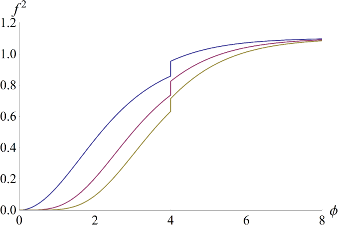
Figure 1: The square of the function $f(\tanh[\varphi/\sqrt{6\alpha}])$ defined in eqs. (1.5) and (1.6), for $\alpha=1$, $A=0.05$, $x_{0}=\tanh[\varphi_{0}/\sqrt{6\alpha}]$ with $\varphi_{0}=4$, and $n=1,2,3$ (from top to bottom).

A different perspective on this issue can be obtained by considering the role of underlying symmetries. A specific framework is provided by the models associated with $\alpha$-attractors in supergravity [17, 18]. A toy model that can serve as a starting point is described by the Lagrangian [18]

$${\cal L}=\sqrt{-g}\left[\frac{1}{2}\partial_{\mu}\chi\partial^{\mu}\chi+\frac{1}{12}\chi^{2}R(g)-\frac{1}{2}\partial_{\mu}\phi\partial^{\mu}\phi-\frac{1}{12}\phi^{2}R(g)-\frac{1}{36}f^{2}(\phi/\chi)\left(\chi^{2}-\phi^{2}\right)^{2}.\right]$$ (1.2)

The model is invariant under the conformal transformation

$$g_{\mu\nu}\to e^{-2\sigma(x)}g_{\mu\nu},~{}~{}~{}~{}~{}~{}\phi\to e^{\sigma(x)}\phi,~{}~{}~{}~{}~{}~{}\chi\to e^{\sigma(x)}\chi.$$ (1.3)

An interesting point is that, for constant $f(\phi/\chi)$, the model possesses a global $SO(1,1)$ symmetry that leaves $\chi^{2}-\phi^{2}$ invariant. The field $\chi$ does not have any physical degrees of freedom and can be eliminated by imposing the gauge-fixing condition $\chi^{2}-\phi^{2}=6$. Following ref. [18], we parametrize the fields as $\chi=\sqrt{6}\cosh(\varphi/\sqrt{6})$, $\phi=\sqrt{6}\sinh(\varphi/\sqrt{6})$. The Lagrangian becomes

$${\cal L}=\sqrt{-g}\left[\frac{1}{2}R(g)-\frac{1}{2}\partial_{\mu}\varphi\partial^{\mu}\varphi-f^{2}\left(\tanh\frac{\varphi}{\sqrt{6}}\right)\right].$$ (1.4)

It is apparent that a constant function $f(x)$ corresponds to a cosmological constant. However, its value is not specified by the $SO(1,1)$ symmetry. A possible deformation of the symmetry is obtained by assuming that $f(x)$ takes fixed values over two continuous ranges of $x$, with a rapid transition at a point $x_{0}$ in between. A stronger deformation, which has been used extensively in the literature, assumes that $f(x)$ has a polynomial form. A schematic form of $f(x)$, that displays a steep step and can also lead to power spectrum consistent with the cosmological constraints, is

$$f(x)=x^{n}+A\,\Theta(x-x_{0}).$$ (1.5)

In practice, the step-function can be replaced by a smooth function. In the more general framework of the $\alpha$-attractors [17, 18], the Lagrangian takes the form

$${\cal L}=\sqrt{-g}\left[\frac{1}{2}R(g)-\frac{1}{2}\partial_{\mu}\varphi\partial^{\mu}\varphi-f^{2}\left(\tanh\frac{\varphi}{\sqrt{6\alpha}}\right)\right],$$ (1.6)

with $\alpha$ a free parameter. In fig. 1 we depict the square of the function $f(\tanh[\varphi/\sqrt{6\alpha}])$ defined according to eq. (1.5), for $\alpha=1$, $A=0.05$, $x_{0}=\tanh[\varphi_{0}/\sqrt{6\alpha}]$ with $\varphi_{0}=4$, and $n=1,2,3$ (from top to bottom).

Our aim is to analyse the power spectra resulting from inflaton potentials with the step feature displayed in fig. 1. We do not consider a specific model, but keep only a minimal number of terms in the inflaton potential. The first term corresponds to vacuum energy, for which we make the crucial assumption that it can have one or more transition points at which it jumps from one constant value to another. We also include a linear term, because it is the only term in a field expansion that is indispensable for our discussion. We neglect the effect of higher powers of the inflaton field that would make the analysis model dependent. Adjusting the free parameters can lead to the appearance of either an inflection point or a sharp drop in the potential, thus allowing the comparison of the effects of the two features. The unavoidable drawback of this simplified setup is that the potential is not flexible enough to generate the correct amplitude and tilt of the spectrum in the CMB range, as well as a sufficient number of efoldings. This can be achieved for a potential that includes higher powers of the field. As an example, we analyse a potential inspired by the Starobinsky model [14]. However, we do not engage in detailed model building here, deferring such an investigation to future work.

In the following section we summarize the basic formalism related to the Mukhanov-Sasaki equation. For the numerical analysis it is most convenient to express this equation using the number of efoldings as independent variable. In section 3 we present the results of a numerical calculation of the spectum, as well as an analytical discussion of the appearing features. The final section includes a summary of our findings.

2 The Mukhanov-Sasaki equation

In this section we introduce the relevant quantities and collect the corresponding dynamical equations for the study of the curvature perturbations and their spectrum.

The most general scalar metric perturbation around the Friedmann-Robertson-Walker (FRW) background takes the form [19]

$$ds^{2}=a^{2}(\tau)\left\{(1+2\phi)d\tau^{2}-2B_{,i}\,dx^{i}d\tau-\left((1-2\psi)\delta_{ij}+2E_{,ij}\right)dx^{i}dx^{j}\right\},$$ (2.1)

with $B_{,i}=\partial_{i}B$, $E_{,ij}=\partial_{i}\partial_{j}E$. On this background, one can parametrize the inflaton field as $\varphi(\tau)+\delta\varphi(\tau,x)$ and define a gauge-invariant perturbation as

$$v=a\left(\delta\varphi+\frac{\varphi^{\prime}}{{\cal H}}\psi\right),$$ (2.2)

which satisfies the Mukhanov-Sasaki equation [11]

$$v^{\prime\prime}-\nabla^{2}v-\frac{z^{\prime\prime}}{z}\,v=0,$$ (2.3)

with $z=a\varphi^{\prime}/{\cal H}$. The primes and the Hubble parameter correspond to derivatives with respect to conformal time. The Fourier modes of $v$ satisfy

$$v_{k}^{\prime\prime}(\tau)+\left(k^{2}-\frac{z^{\prime\prime}}{z}\right)v_{k}(\tau)=0.$$ (2.4)

The standard assumption, which we adopt, is that at early times the field is in the Bunch-Davies vacuum. The strong features of the potential have not become relevant yet, so that the background field is in the slow-roll regime. All the modes that are phenomenologically interesting today were deeply subhorizon at such early times. They are described by the standard expression $v_{k}=e^{-ik\tau}/\sqrt{2k}$, which we use in order to set the initial conditions for their subsequent evolution. The spectrum of perturbations becomes more transparent through the use of the gauge-invariant comoving curvature perturbation $R=-v/z$, which satisfies

$$R_{k}^{\prime\prime}+2\frac{z^{\prime}}{z}R_{k}^{\prime}+k^{2}R_{k}=0$$ (2.5)

in Fourier space.

As we are mainly interested in the amplitude of the complex variables $v$ and $R$, we introduce polar coordinates, such that $v_{k}(\tau)={\cal V}_{k}(\tau)\exp(-i\theta_{k}(\tau))$, with ${\cal V}_{k}$ and $\theta_{k}$ real. From eq. (2.4) we obtain

$${\cal V}_{k}^{\prime\prime}+\left(k^{2}-\frac{z^{\prime\prime}}{z}-\theta_{k}^{\prime 2}\right){\cal V}_{k} = 0$$ (2.6)

$$\frac{\theta_{k}^{\prime\prime}}{\theta_{k}^{\prime}}+2\frac{{\cal V}_{k}^{\prime}}{{\cal V}_{k}} = 0.$$ (2.7)

The second equation can be integrated, with the solution $\theta_{k}^{\prime}\,{\cal V}_{k}^{2}={\rm constant}$ At early times we have ${\cal V}_{k}=1/\sqrt{2k}$ and $\theta_{k}=k\tau$. This fixes the constant of integration to 1/2, so that we can set

$$\theta_{k}^{\prime}=\frac{1}{2{\cal V}_{k}^{2}}$$ (2.8)

in eq. (2.6). In this way we obtain

$${\cal V}_{k}^{\prime\prime}+\left(k^{2}-\frac{z^{\prime\prime}}{z}-\frac{1}{4{\cal V}_{k}^{4}}\right){\cal V}_{k}=0,$$ (2.9)

which must be solved with initial conditions ${\cal V}_{k}\to 1/\sqrt{2k}$, ${\cal V}_{k}^{\prime}\to 0$, for $\tau\to-\infty$. The curvature perturbation is parametrized as $R_{k}(\tau)=-{\cal R}_{k}(\tau)\exp(-i\theta_{k}(\tau))$, with ${\cal R}_{k}={\cal V}_{k}/z$. Its amplitude satisfies

$${\cal R}_{k}^{\prime\prime}+2\frac{z^{\prime}}{z}{\cal R}_{k}^{\prime}+\left(k^{2}-\frac{1}{4z^{4}{\cal R}_{k}^{4}}\right){\cal R}_{k}=0.$$ (2.10)

It is convenient for the numerical analysis to use the number of efoldings $N$ as the independent variable for the evolution of the perturbations. The Hamilton-Jacobi slow-roll parameters are defined through the relations

$$H^{2} = \frac{V(\varphi)}{3M_{\rm Pl}^{2}-\frac{1}{2}\varphi_{,N}^{2}}$$ (2.11)

$$\varepsilon_{H} = -\frac{d\ln H}{dN}=\frac{\varphi^{2}_{,N}}{2M_{\rm Pl}^{2}}$$ (2.12)

$$\eta_{H} = \varepsilon_{H}-\frac{1}{2}\frac{d\ln\varepsilon_{H}}{dN}=\frac{\varphi^{2}_{,N}}{2M_{\rm Pl}^{2}}-\frac{\varphi_{,NN}}{\varphi_{,N}},$$ (2.13)

where $H=e^{-N}{\cal H}$ is the Hubble parameter defined through cosmic time, and subscipts denote derivatives with respect to $N$. The parameter $z$ is given by

$$z=e^{N}\,\varphi_{,N},$$ (2.14)

while the effective equation of state for the background is $w=-1+2\varepsilon_{H}/3$.

The evolution of the background field is governed by the equation

$$\varphi_{,NN}+3\varphi_{,N}-\frac{1}{2M_{\rm Pl}^{2}}\varphi_{,N}^{3}+\left(3M_{\rm Pl}^{2}-\frac{1}{2}\varphi_{,N}^{2}\right)\frac{V_{,\varphi}}{V}=0,$$ (2.15)

with $V(\varphi)$ the inflaton potential. The inflaton fluctuation obeys the equation

$$v_{k,NN}+(1-\varepsilon_{H})v_{k,N}+\left(\frac{k^{2}}{e^{2N}H^{2}}+(1+\varepsilon_{H}-\eta_{H})(\eta_{H}-2)-(\varepsilon_{H}-\eta_{H})_{,N}\right)v_{k}=0,$$ (2.16)

and its amplitude

$${\cal V}_{k,NN}+(1-\varepsilon_{H}){\cal V}_{k,N}+\left(\frac{k^{2}}{e^{2N}H^{2}}\left(1-\frac{1}{4k^{2}{\cal V}_{k}^{4}}\right)+(1+\varepsilon_{H}-\eta_{H})(\eta_{H}-2)-(\varepsilon_{H}-\eta_{H})_{,N}\right){\cal V}_{k}=0.$$ (2.17)

In the above differential equations we can express the coefficients as

$$1-\varepsilon_{H} = 1-\frac{\varphi^{2}_{,N}}{2M_{\rm Pl}^{2}}$$ (2.18)

$$(1+\varepsilon_{H}-\eta_{H})(\eta_{H}-2)-(\varepsilon_{H}-\eta_{H})_{,N} = -2-3\frac{\varphi_{,NN}}{\varphi_{,N}}-\frac{\varphi_{,NNN}}{\varphi_{,N}}+\frac{\varphi_{,N}^{2}}{2M_{\rm Pl}^{2}}+\frac{\varphi_{,N}\,\varphi_{,NN}}{2M_{\rm Pl}^{2}}.$$ (2.19)

We can also write equivalent equations for the curvature perturbation, which take the form

$$R_{k,NN}+\left(3+\frac{2\varphi_{,NN}}{\varphi_{,N}}-\frac{\varphi_{,N}^{2}}{2M_{\rm Pl}^{2}}\right)R_{k,N}+\frac{k^{2}}{e^{2N}H^{2}}R_{k}=0$$ (2.20)

and

$${\cal R}_{k,NN}+\left(3+\frac{2\varphi_{,NN}}{\varphi_{,N}}-\frac{\varphi_{,N}^{2}}{2M_{\rm Pl}^{2}}\right){\cal R}_{k,N}+\frac{k^{2}}{e^{2N}H^{2}}\left(1-\frac{1}{4k^{2}e^{4N}\varphi_{,N}^{4}{\cal R}_{k}^{4}}\right){\cal R}_{k}=0,$$ (2.21)

for the perturbation and its amplitude, respectively.

The spectrum of curvature perturbations is

$$\Delta_{R}^{2}=\frac{k^{3}}{2\pi^{2}}\frac{{\cal V}_{k}^{2}}{e^{2N}\varphi_{,N}^{2}}=\frac{k^{3}}{2\pi^{2}}{\cal R}_{k}^{2}.$$ (2.22)

The normalization of the spectrum can be set in terms of a pivot scale $k_{*}$ and the number of efoldings $N_{*}$ at which it crosses the horizon: $k_{*}=e^{N_{*}}H_{*}$. By defining dimensionless variables ${\tilde{k}}=k/k_{*}$, ${\tilde{v}}_{k}=\sqrt{k_{*}}\,v_{k}$, $\tilde{\cal V}_{k}=\sqrt{k_{*}}\,{\cal V}_{k}$, $\tilde{R}_{k}=\sqrt{k_{*}}\,R_{k}$, $\tilde{\cal R}_{k}=\sqrt{k_{*}}\,{\cal R}_{k}$, as well as ${{\delta N}}=N-N_{*}$, we obtain

$$\Delta_{R}^{2}=A_{s}\frac{{\tilde{k}}^{3}\,2\tilde{\cal V}_{k}^{2}}{e^{2\,{{\delta N}}}}\frac{\varphi_{,N*}^{2}}{\varphi_{,N}^{2}}.$$ (2.23)

where

$$A_{s}=\frac{1}{4\pi^{2}}\frac{H^{2}_{*}}{\varphi^{2}_{,N*}}$$ (2.24)

sets the scale for the amplitude.

For a given inflaton potential, one can integrate numerically eq. (2.15) in order to derive the inflaton background, and then integrate one of eqs. (2.16), (2.17), (2.20), (2.21) for the field or curvature perturbation, in order to deduce the spectrum. The real and imaginary parts of $v_{k}$ and $R_{k}$ oscillate very rapidly for subhorizon perturbations, as can be deduced from eqs. (2.16), (2.20). This makes the numerical integration of these equations more demanding. On the other hand, the amplitudes ${\cal V}_{k}$ and ${\cal R}_{k}$ have a smoother evolution. It is possible for these quantities to become oscillatory also, as we shall see in the following. However, the presence of the terms $\sim{\cal V}_{k}^{-4}$ in eq. (2.17) and $\sim{\cal R}_{k}^{-4}$ in eq. (2.21) guarantees that these amplitudes remain always positive. For the numerical analysis of the following sections, we solve the evolution equations both for the field perturbation $v_{k}$ and its amplitude ${\cal V}_{k}$ in order to cross-check the results.

A quantity that plays a crucial role in determining the qualitative behaviour of the solutions is the one in the first parenthesis of eqs. (2.20), (2.21), which we denote by

$$f(N)=3+\frac{2\varphi_{,NN}}{\varphi_{,N}}-\frac{\varphi_{,N}^{2}}{2M_{\rm Pl}^{2}}$$ (2.25)

as a function of $N$. In the slow-roll regime, this quantity acts as a generalized friction term. However, for the more general evolution that we are considering, it may become negative and lead to a dramatic enhancement of the perturbations. We also define the function

$$g(N)=1-\frac{1}{4k^{2}e^{4N}\varphi_{,N}^{4}{\cal R}_{k}^{4}},$$ (2.26)

appearing in the second parenthesis, evaluated on a given solution for the perturbation. This function diverges whenever the amplitude ${\cal R}_{k}$ approaches zero, thus preventing it from turning negative. An alternative way to view this point is to notice that eq. (2.21) is equivalent to eq. (2.20), while the amplitude of $R_{k}$ cannot turn negative. The fact that ${\cal R}_{k}$ can approach zero at certain times during the later stages of the evolution, as we shall see in the following, indicates that during these stages the real and the imaginary part of $R_{k}$ are in phase and can cross zero almost simultaneously.

3 Features of the inflaton potential

We would like to explore features of the inflaton potential that can result in an amplification of the spectrum of curvature perturbations by several orders of magnitude. Our underlying motivation is to determine the appropriate conditions for the creation of primordial black holes. This is possible in a range of scales in which perturbations become of order one. Significant deviations from the scale-invariant spectrum can occur only at small length scales (large wavenumbers), for which the evolution of the spectrum is highly nonlinear, so that current observations do not constrain its form severely. Such scales correspond to comoving wavenumbers larger than ${\cal O}(1)$ in units of Mpc^-1.

3.1 Minimal framework

Figure 2: The inflaton potential $V(\varphi)$ of eq. (3.1), the evolution of the inflaton $\varphi$, the function $f(N)$ defined in eq. (2.25), and the power spectrum of curvature perturbations with wavenumber $k$, for various choices of the parameters of the potential: First row: $A_{1}=0.000605$, $c_{i}=100$, $B=-0.03$.  Second row: $A_{1}=-0.3$, $c_{i}=20$, $B=-0.03$.  Third row: $A_{1}=-0.3$, $c_{i}=100$, $B=-0.03$.  Fourth row: $A_{1}=-0.3$, $c_{i}=300$, $B=-0.03$. The scales of $k$ and $V$ are arbitrary.

Instead of considering a specific model, we keep only the minimal number of elements required for addressing the problem. We focus on only a limited range of scales, and the corresponding values of the inflaton background when these exit the horizon. We approximate the inflaton potential by the smallest number of relevant terms. The features of interest are:

1. an inflection point, at which the first and second derivatives of the potential vanish,

2. one or more points at which the potential decreases sharply.

Both these features can appear in a potential with the simple parameterization

$$V(\varphi)=V_{0}\left(1+\frac{1}{2}\sum_{i}A_{i}\left(1+\tanh(c_{i}(\varphi-\varphi_{i}))\right)+B\varphi\right),$$ (3.1)

where $i$ is a positive integer counting certain special field values. The first terms in the parenthesis can be identified with the vacuum energy that drives inflation. The crucial assumption that we have made is that the vacuum energy can have one or more transition points at which it jumps from one constant value to another. As we discussed in the introduction, one could speculate that these points correspond to values of the inflaton background associated with some kind of decoupling of modes whose quantum fluctuations contribute to the vacuum energy. However, such a speculation cannot be put easily on formal ground because of our lack of understanding of the nature of the cosmological constant. Sharp changes in the vacuum energy can also occur during transitions from one region of a multi-field potential to another. The analysis of such a system would require the inclusion of entropy perturbations. The current work is a simplified first step towards understanding the features that could appear in the spectrum of curvature perturbations for a multi-field system. The linear term in the potential (3.1) is the only term in a field expansion that is indispensable for our discussion. In this subsection we neglect the effect of higher powers of the inflaton field that would make the analysis model dependent. We assume, without loss of generality, that $B<0$. An inflection point can appear at $\phi_{1}=0$ if $A_{1}=-2B/c$, $A_{i}=0$ for $i>1$. Negative values of $A_{i}$ result in a series of steps in the potential.

Figure 3: The inflaton potential $V(\varphi)$ of eq. (3.1), the evolution of the inflaton $\varphi$, the function $f(N)$ defined in eq. (2.25), and the power spectrum of curvature perturbations with wavenumber $k$, for various choices of the parameters of the potential: First row: $A_{1}=-0.3$, $c_{i}=100$, $B=-0.03$.  Second row: $A_{1}=-0.15$, $A_{2}=-0.15$, $\varphi_{2}=0.3$, $c_{i}=100$, $B=-0.03$.  Third row: $A_{1}=-0.1$, $A_{2}=-0.1$, $A_{3}=-0.1$, $\varphi_{2}=0.3$, $\varphi_{3}=0.6$, $c_{i}=100$, $B=-0.03$. The scales of $k$ and $V$ are arbitrary.

A drawback of the potential (3.1) is that it is not possible to make a connection with the range of the spectrum that is relevant for the cosmic-microwave-background (CMB). The slope $B$ of the potential required for agreement with the measured spectral index is too steep for obtaining a large number of efoldings. As a result, contact with the observations is not possible and we treat the pivot scale $k_{*}$, the amplitude $A_{s}$ and the spectral index $n_{s}$, introduced in the previous section, as free parameters. In particular, we assume that $k_{*}$ is located deep in the nonlinear part of the spectrum and the spectral index is sufficiently close to 1 for a large number of efoldings to be produced. We present our results for the spectrum in units of $A_{s}$, which is equivalent to setting $A_{s}=1$. It is also obvious from eq. (2.15) that the absolute scale $V_{0}$ of the potential does not play any role for our considerations. In practice, we set $V_{0}=1$ for the numerical analysis. Finally, the inflaton field and the constants $c_{i}$, $B$ can be given in units of $M_{\rm Pl}$, which is equivalent to setting $M_{\rm Pl}=1$ in eq. (2.15).

Before computing the spectrum, it is instructive to understand which type of background evolution leads to its enhancement. The perusal of eq. (2.21) leads to the conclusion that the sign of the function $f(N)$ defined in eq. (2.25) is crucial. For $f(N)>0$ the second term of eq. (2.21) acts as a friction term, suppressing the growth of the curvature perturbation. The opposite happens for $f(N)<0$. It is known that the presence of an inflection point in the potential enhances the spectrum. For this reason, we examine first the form of $f(N)$ for such a case. Then we analyse the conditions under which a similar enhancement of the spectrum can occur for a potential with a step-like structure. It must be emphasized that the two cases are distinct. The rolling of the inflaton through an inflection point does not stop inflation, even though the standard slow-roll conditions are not satisfied because of the large value of $\eta_{H}$. On the other hand, the transition through a sharp drop in the potential leads to a fast increase of the time-derivative of the inflaton, and in many cases to a brief interruption of inflation. This is apparent from the effect of a large value of $\varepsilon_{H}$ on the effective equation-of-state parameter $w=2\varepsilon_{H}/3-1$.

Figure 4: The inflaton potential $V(\varphi)$ of eq. (3.1), the evolution of the inflaton $\varphi$, the function $f(N)$ defined in eq. (2.25), and the power spectrum of curvature perturbations with wavenumber $k$, for various choices of the parameters of the potential: First row: $A_{1}=-0.1$, $A_{2}=-0.1$, $A_{3}=-0.1$, $\varphi_{2}=0.2$, $\varphi_{3}=0.4$, $c_{i}=100$, $B=-0.03$.  Second row: $A_{1}=-0.1$, $A_{2}=-0.1$, $A_{3}=-0.1$, $\varphi_{2}=0.3$, $\varphi_{3}=0.6$, $c_{i}=100$, $B=-0.03$.  Third row: $A_{1}=-0.1$, $A_{2}=-0.1$, $A_{3}=-0.1$, $\varphi_{2}=0.4$, $\varphi_{3}=0.8$, $c_{i}=100$, $B=-0.03$. The scales of $k$ and $V$ are arbitrary.

In fig. 2 we present various elements of the calculation of the power spectrum for different potentials. We have used the same scale for all related plots in order to make the comparison easy. The first plot in each row depicts the inflaton potential. The potential at the top has an inflection point at $\varphi=0$, even though this is not clearly visible. The potentials in the next three rows display a step at $\varphi=0$, whose steepness is increased from top to bottom by choosing larger values of the parameter $c_{1}$. The form of the potential is reflected in the field evolution. In the second plot of the first row, the field stays almost constant near zero for several efoldings. In the following rows it evolves very quickly, within 2-3 efoldings, from one plateau of the potential to the next. The third plot in each row depicts the “effective friction” $f(N)$. In all cases this function becomes negative during part of the evolution, thus leading to a strong enhancement of the fluctuations. For an inflection point it starts with the standard value 3, then becomes negative, returns to positive values larger than 3, and eventually becomes equal to 3 again. For a step in the potential, there is a strong increase to very large positive values before the function becomes negative. This increase is confined within a period of efoldings that shrinks with increasing steepness (and $c_{1}$). On the other hand, the form of $f(N)$ in the interval where it is negative is largely independent of $c_{1}$, because it is determined by the approach of the field to slow roll on the second plateau. It seems reasonable to expect that, for steeper steps, the suppression of the perturbation during the strong increase of $f(N)$ is a subleading effect relative to the subsequent enhancement. This expectation is confirmed by the spectrum depicted in the last plot of each row. In the first row we observe the strong and broad enhancement of the spectrum associated with an inflection point. After an initial dip, the spectrum grows rather steeply towards a maximum, beyond which it decays smoothly towards its almost scale-invariant form. This behavior is consistent with the general analysis of ref. [21]. The spectra of the next three rows display a strong oscillatory behaviour, which will be discussed in the following. The largest enhancement is achieved for a band of wavenumbers during the first oscillation. It is clear that the magnitude of this enhancement increases with $c_{1}$.

The maxima of the spectra in fig. 2 are larger by up to three orders of magnitude relative to the standard value for the scale-invariant case. The enhancement is restricted by the fact that the maximal “velocity” achieved by the rolling field is limited by the size of the step. It is possible, however, that the potential includes several step-like features. We examine their effect in fig. 3, where we compare potentials with one, two or three steps. The total drop in the potential is the same in all three cases. It is apparent from the last column that the presence of several features in the potential can lead to the increase of the spectrum by several orders of magnitude. The reason can be traced to the “effective friction” $f(N)$, displayed in the third column. The presence of several steps increases the total number of efoldings over which this function takes negative values. This is reflected in the larger enhancement of the perturbations.

The field values at which the features of the potential appear play a crucial role for the form of the resulting spectrum. This feature is demonstrated in fig. 4 in which we consider potentials with three steps, at field values with increasing distance from each other. It is apparent from the first row that when the steps are very close to each other the function $f(N)$ stays negative for a small number of efoldings and the enhancement is comparable to the one-step case. Increasing the distance leads to spectrum enhancement, as $f(N)$ stays negative longer. However, the enhancement persists up to a certain distance between the features of the potential, beyond which each step acts independently on the spectrum. This beaviour is apparent in the second and third rows of fig. 4.

   

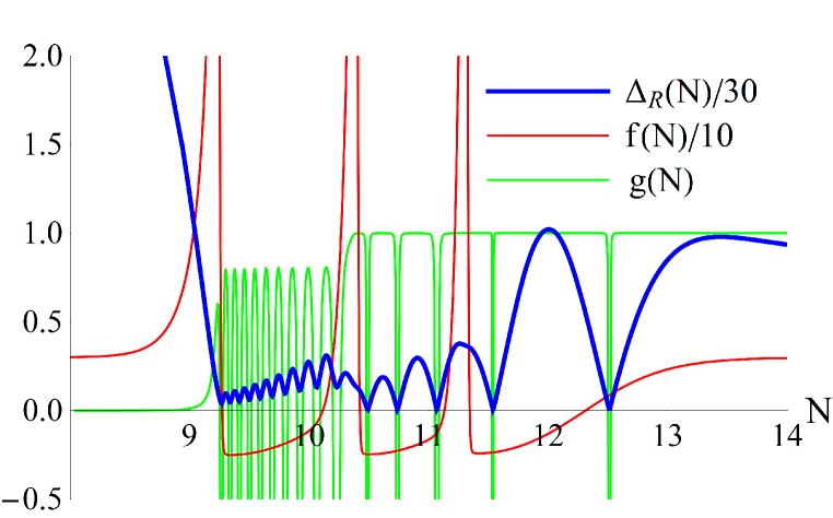
Figure 5: The curvature perturbation as a function of the number of efoldings $N$, and the functions $f(N)$, $g(N)$, for the potential (3.1) with $A_{1}=-0.1$, $A_{2}=-0.1$, $A_{3}=-0.1$, $\varphi_{2}=0.3$, $\varphi_{3}=0.6$, $c=100$, $B=-0.03$.  Blue line: $\frac{1}{30}\sqrt{\Delta^{2}_{R}(k,N)}$ for $k=2.66\times 10^{5}$.  Red line: The function $\frac{1}{10}f(N)$ defined in (2.25).  Green line: The function $g(N)$ defined in (2.26). 

A prominent feature of the spectra resulting from sharp drops in the inflaton potential is the appearance of strong oscillations, whose origin we would like to understand. One can speculate that the oscillatory pattern arises when modes within a wavenumber range exit the horizon, but then reenter during the period when inflation stops and the comoving horizon grows. Upon reentry they start oscillating again, until they exit for a second time during a subsequent period of inflation [19, 20]. However, the onset or freezing of the oscillatory behaviour is not instantaneous, while the crossing of the horizon is essentially a continuous process with a certain width. An exact analytical treatment is difficult, and the evolution of each mode can be computed only numerically. In fig. 5 we present the evolution of the curvature perturbation $\tilde{\cal R}_{\tilde{k}}(N)$ (blue line) for a given Fourier mode ${\tilde{k}}=2.66\times 10^{5}$ for an inflaton background arising from a potential with three steps. The red and green lines depict the functions $f(N)$ and $g(N)$ defined by eqs. (2.25) and (2.26), respectively. The enhancement of the curvature perturbation during the periods of inflation with negative $f(N)$ is apparent. Similarly, the freezing of the perturbation during the periods with positive $f(N)$ is also apparent, resulting in $\tilde{\cal R}_{\tilde{k}}(N)$ becoming asymptotically constant.

A striking feature is the series of oscillations for the amplitude of perturbations, which approaches zero at several values of $N$. At these points the function $g(N)$ becomes very negative, thus preventing the amplitude from crossing zero. The origin of the oscillations can be understood if one considers eq. (2.20) for constant $f(N)=\kappa$. Its solution involves a linear combination of the Bessel functions $J_{\pm\kappa/2}$ and has the form

$$R_{k}(N)=Ae^{-\frac{1}{2}\kappa\,N}\left(J_{\kappa/2}\left(e^{-N}\frac{k}{H}\right)+c\,J_{-\kappa/2}\left(e^{-N}\frac{k}{H}\right)\right).$$ (3.2)

The initial subhorizon evolution of the perturbation during the slow-roll regime corresponds to the solution with $\kappa=3$ and $c=i$. This particular choice of $c$ eliminates the oscillatory behaviour in the amplitude of $R_{k}(N)$. However, the nontrivial background evolution that we are considering corresponds to a varying $\kappa$, as well as a varying relative coefficient of the Bessel functions. As a result the zeros of the Bessel functions become apparent in the amplitude ${\cal R}_{k}(N)$, which becomes very small for $e^{-N}k/H$ approaching one of these zeros. The asymptotic value of ${\cal R}_{k}$ for large $N$ depends on the time of the transition of the background solution to positive values of $f(N)$. The freezing of $R_{k}$ can occur at any stage of the oscillatory cycle, depending on the value of $k$. Eventually, this is reflected in the strong oscillatory behaviour of the spectrum as a function of $k$.

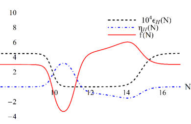
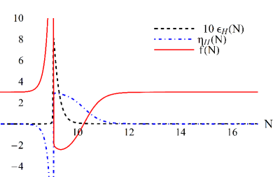
Figure 6: The Hamilton-Jacobi slow-roll parameters $\epsilon_{H}$ and $\eta_{H}$, defined in eqs. (2.12) and (2.13) respectively, and the “effective-friction” term $f(N)$ defined in eq. (2.25), as a function of the number of efoldings, for two choices of the parameters of the potential: Left plot: $A_{1}=0.000605$, $c_{1}=100$, $B=-0.03$.  Right plot: $A_{1}=-0.3$, $c_{1}=100$, $B=-0.03$. The two sets of parameters correspond to the first and third row of fig. 2.

In fig. 6 we look in detail at the role of the slow-roll parameters in the enhancement of the spectrum. We contrast the case of an inflection point in the potential (left plot) with that of a step-like feature (right plot). In the first case, the solution remains inflationary during the whole evolution. The Hamilton-Jacobi parameter $\epsilon_{H}$ has a constant value, apart from the part of the evolution near the inflection point, during which it approaches zero. The parameter $\eta_{H}$ starts from a value close to zero during the slow-roll regime, first turns positive and subsequently negative, eventually returning close to zero during the second slow-roll regime. The “effective-friction” term is strongly influenced by $\eta_{H}$ and becomes negative during the time that $\eta_{H}$ is significantly larger than zero. In the case of a step-like feature, the parameter $\epsilon_{H}$ grows large during the interval that this feature is transversed. For sharp steps or when the second plateau is sufficiently low, the solution ceases to be inflationary for a short time, as can be verified by computing the equation of state parameter $w=-1+2\epsilon_{H}/3$. The parameter $\eta_{H}$ first turns negative, but then positive as the inflaton “decelerates” while settling on a slow-roll regime on the second plateau. The “effective friction” is again mainly influenced by $\eta_{H}$ and becomes negative when $\eta_{H}$ takes large positive values. The effect is sufficiently strong for the friction term to be negative even when $\epsilon_{H}$ is of order 1.

3.2 A specific model

Figure 7: The inflaton potential $V(\varphi)$ defined in (3.3), the evolution of the inflaton $\varphi$ as a function of the number of efoldings $N$, the function $f(N)$ defined in eq. (2.25), and the power spectrum of curvature perturbations with wavenumber $k$, for $A_{1}=A_{2}=A_{3}=0.05$, $c_{1}=c_{2}=c_{3}=200$, $\varphi_{1}=5$, $\varphi_{2}=4.8$, $\varphi_{3}=4.6$, $B=-\sqrt{2/3}$. Dimensionful parameters in units of $M_{\rm Pl}$. The scale of the potential $V_{0}$ has been adjusted in order to reproduce the amplitude of curvature perturbations in the CMB range.

The analysis of the previous subsection relied on a simplified potential which did not allow us to make contact with the physical scales of the power spectrum. In order to obtain a more complete picture we study in this subsection a potential inspired by the Starobinsky model [14], to which we introduce step-like features. The potential is given by the expression

$$V(\varphi)=V_{0}\left(1-e^{B\varphi}\right)^{2}\left(1+\frac{1}{2}\sum_{i}A_{i}\left(1+\tanh(c_{i}(\varphi-\varphi_{i}))\right)\right).$$ (3.3)

As we do not engage in model building in this work, the above potential has not been derived from a more fundamental framework, such as supergravity. It is a phenomenological construction that has enough flexibility to allow for a sufficient number of efoldings, as well as power-spectrum scale and spectral index compatible with the CMB observations.

In fig. 7 we present the various elements in the calculation of the power spectrum of curvature perturbations for this model. The first plot depicts the potential with the characteristic step-like feature. The values of the parameters are: $A_{1}=A_{2}=A_{3}=0.05$, $c_{1}=c_{2}=c_{3}=200$, $\varphi_{1}=5$, $\varphi_{2}=4.8$, $\varphi_{3}=4.6$, $B=-\sqrt{2/3}$. Dimensionful parameters are given in units of $M_{\rm Pl}$. The evolution of the inflaton $\varphi$ as a function of the number of efoldings $N$ is shown in the second plot. We count the number of efoldings from the moment that the scale with wavenumber $k_{*}=0.05\,{\rm Mpc}^{-1}$, which we use as a pivot scale, exits the horizon. The above parameters result in a power spectrum in the CMB range with a spectral index $n_{s}\simeq 0.969$ and a tensor to scalar ratio $r\simeq 0.0027.$ The third plot depicts the “effective-friction” function $f(N)$ defined in eq. (2.25). It deviates from the standard value 3 during the period in which the inflaton field takes values in the vicinity of the step-like feature of the potential. When $f(N)$ is negative, it acts as negative friction, leading to the enhancement of the curvature modes that cross the horizon during this period. The enhancement for certain wavenumber bands can be significant. For this paticular choice of parameters the spectrum is enhanced by roughly four orders of magnitude. The enhancement can be made larger with an appropriate choice of the potential, or with the inclusion of additional step-like features. The curvature power spectrum is depicted in the last plot. It has been normalized to the standard value $\simeq 2.1\times 10^{-9}$ for $k_{*}=0.05\,{\rm Mpc}^{-1}$ through an appropriate choice of the scale $V_{0}$ of the potential.

The strong features in the spectrum appear deep in the nonlinear region, where the phenomenological constraints are not strict because of the lack of analytical understanding of the evolution of the perturbations. The approximate wavenumber value $k_{f}$ for which these features appear can be estimated by noting that $k_{f}=\exp(N_{f})H_{f}$ must hold at horizon crossing. For the pivot scale this relation is $k_{*}=\exp(N_{*})H_{*}$, and we have set $N_{*}=0$. If the Hubble parameter does not change substantially between $N_{*}$ and $N_{f}$, we have $k_{f}/k_{*}\sim\exp(N_{f})$. From the second plot of fig. 7 we obtain $N_{f}\sim 23$, which gives $k_{f}\sim 10^{9}\,{\rm Mpc}^{-1}$, in agreement with the last plot.

4 Conclusions

We explored the possible enhancement of the power spectrum of curvature perturbations in single-field inflation when particular features appear in the inflaton potential. Our motivation stems from the possibility that a strong enhancement of the spectrum within a range of wavenumbers may have resulted in the copious production of primordial black holes. One characteristic feature that is known to induce the enhancement of the spectrum is an inflection point of the potential at some value of the inflaton field [8]. We analysed here the opposite case, i.e. a sharp decrease of the potential, which may result even in the interruption of inflation in certain cases, in contrast to what happens around an inflection point. Therefore, it comes as a surprise that the fast “rolling” of the inflaton field through such a feature can have as a consequence the enhancement of the fluctuations. Building on previous work [6], we explored the conditions under which the enhancement can be very large, by several orders of magnitude relative to its magnitude within the almost scale-invariant range. It must be noted that it is always possible to enhance the spectrum by engineering the transition to a second very flat plateau of the potential. The time derivative of the inflaton under slow-roll conditions on the plateau would be very small, resulting in an enhanced power spectrum. In our analysis we exclude this rather trivial possibility by keeping the slope rougly constant, apart from at the transition point or points, and focus on the effect of the transition itself.

We analysed in detail the simplified potential of eq. (3.1). We found that sharp transitions lead to the strong growth of the curvature perturbation. The reason can be traced to the “effective-friction” term of eq. (2.20), which is given by the function $f(N)$ defined in eq. (2.25). Even though this function is positive during the first part of the transition, thus suppressing the perturbation, it can become negative during the second part, when the inflaton approaches slow roll on the second plateau, and can lead to a dramatic enhancement. The main effect comes from the slow-roll parameter $\eta_{H}$ taking large positive values, even when the parameter $\epsilon_{H}$ is large. The effect is increased by the steepness of the potential, but is also limited by the size of the potential drop that bounds the maximal inflaton “velocity”. However, successive nearby steps give an additive effect, leading to a spectrum enhancement by several orders of magnitude. We discussed up to three steps, but increasing this number can increase the enhancement arbitrarily.

The second prominent feature of the spectrum is its strong oscillatory form as a function of wavenumber. We analysed the origin of this feature during the discussion of fig. 5 in the previous section. The appearance of wavenumber bands in which the spectrum takes very large values can lead to the creation of primordial black holes of characteristic sizes when the corresponding fluctuations enter the horizon. The suppression of the spectrum in other bands indicates the absence of black holes of other sizes. The combined effect can lead to a very distinctive pattern.

Another very exciting prospect is the possibility of detecting the oscillatory pattern in the spectrum of gravitational waves generated through the scalar perturbations at second order [22]. This scenario is independent of the creation of primordial black holes and becomes possible even for a milder enhancement of the spectrum. The detection of stochastic gravitational waves is a portal to the primordial spectrum of scalar perturbations at small scales and can be used in order to look for strong features in the inflationary dynamics. The oscillatory patterns appearing in the scenario we discussed provide a prime example of a possibly detectable feature. Because of a double integration over momenta in the expression for the spectrum of gravitational waves, the oscillatory pattern is expected to be superimposed on a smooth underlying curve with one or two peaks [23]. However, a clear distinction is possible between smooth spectra resulting from an inflection point in the inflaton potential and the oscillatory spectra in our scenario. It must be noted that such oscillatory features have been considered recently for the spectra resulting from two-field inflationary models [24].

A realistic inflaton potential must generate a sufficient number of efoldings and result in a spectrum consistent with the CMB constraints. Even though our aim here was not to engage in detailed model building, we discussed the potential of eq. (3.3), which is inspired by the Starobinsky model [14]. The potential is constructed in a rather artificial manner and can serve only as a toy model. However, it is very useful in order to establish that the type of spectrum enhancement that we are suggesting can appear in realistic setups. One particular property of the potentials that we are considering is their dependence on the hyperbolic tangent of the field. As we discussed in the introduction, this occurs in models associated with $\alpha$-attractors in supergravity [17, 18], in which the function $\tanh(\varphi/\sqrt{\alpha})$ becomes part of the potential in the Einstein frame. The study of the spectra of density perturbations and induced gravitational waves in specific models will be the subject of future work.

References

-
[1]
B. Abbott et al. [LIGO Scientific and Virgo],
Phys. Rev. Lett. 116 (2016) no.6, 061102
[arXiv:1602.03837 [gr-qc]];
B. P. Abbott et al. [LIGO Scientific and Virgo], Phys. Rev. Lett. 116 (2016) no.24, 241103 [arXiv:1606.04855 [gr-qc]];
B. P. Abbott et al. [LIGO Scientific and Virgo], Phys. Rev. Lett. 118 (2017) no.22, 221101 [arXiv:1706.01812 [gr-qc]];
B. P. Abbott et al. [LIGO Scientific and Virgo], Astrophys. J. 851 (2017) no.2, L35 [arXiv:1711.05578 [astro-ph.HE]];
B. Abbott et al. [LIGO Scientific and Virgo], Phys. Rev. Lett. 119 (2017) no.14, 141101 [arXiv:1709.09660 [gr-qc]]. -
[2]
Ya. B. Zeldovich and I. D. Novikov,
Sov. Astron. -AJ 10 (1967) 602;
S. Hawking, Mon. Not. Roy. Astron. Soc. 152 (1971) 75;
B. J. Carr and S. W. Hawking, Mon. Not. Roy. Astron. Soc. 168 (1974) 399;
B. J. Carr, Astrophys. J. 201 (1975), 1-19. -
[3]
B. Carr, F. Kuhnel and M. Sandstad,
Phys. Rev. D 94 (2016) no.8, 083504
[arXiv:1607.06077 [astro-ph.CO]];
M. Sasaki, T. Suyama, T. Tanaka and S. Yokoyama, Class. Quant. Grav. 35 (2018) no.6, 063001 [arXiv:1801.05235 [astro-ph.CO]];
B. Carr, K. Kohri, Y. Sendouda and J. Yokoyama, [arXiv:2002.12778 [astro-ph.CO]];
B. Carr and F. Kuhnel, [arXiv:2006.02838 [astro-ph.CO]];
A. M. Green and B. J. Kavanagh, [arXiv:2007.10722 [astro-ph.CO]]. -
[4]
C. Germani and T. Prokopec,
Phys. Dark Univ. 18 (2017), 6-10
[arXiv:1706.04226 [astro-ph.CO]];
H. Motohashi and W. Hu, Phys. Rev. D 96 (2017) no.6, 063503 [arXiv:1706.06784 [astro-ph.CO]]. - [5] P. Ivanov, P. Naselsky and I. Novikov, Phys. Rev. D 50 (1994), 7173-7178.
-
[6]
J. A. Adams, B. Cresswell and R. Easther,
Phys. Rev. D 64 (2001), 123514
[arXiv:astro-ph/0102236 [astro-ph]];
S. M. Leach and A. R. Liddle, Phys. Rev. D 63 (2001), 043508 [arXiv:astro-ph/0010082 [astro-ph]];
S. M. Leach, M. Sasaki, D. Wands and A. R. Liddle, Phys. Rev. D 64 (2001), 023512 [arXiv:astro-ph/0101406 [astro-ph]]. -
[7]
S. Clesse and J. García-Bellido,
Phys. Rev. D 92 (2015) no.2, 023524
[arXiv:1501.07565 [astro-ph.CO]];
M. Kawasaki, A. Kusenko, Y. Tada and T. T. Yanagida, Phys. Rev. D 94 (2016) no.8, 083523 [arXiv:1606.07631 [astro-ph.CO]];
K. Inomata, M. Kawasaki, K. Mukaida, Y. Tada and T. T. Yanagida, Phys. Rev. D 96 (2017) no.4, 043504 [arXiv:1701.02544 [astro-ph.CO]]. -
[8]
J. Garcia-Bellido and E. Ruiz Morales,
Phys. Dark Univ. 18 (2017), 47-54
[arXiv:1702.03901 [astro-ph.CO]];
J. M. Ezquiaga, J. Garcia-Bellido and E. Ruiz Morales, Phys. Lett. B 776 (2018), 345-349 [arXiv:1705.04861 [astro-ph.CO]];
H. Di and Y. Gong, JCAP 07 (2018), 007 [arXiv:1707.09578 [astro-ph.CO]];
K. Kannike, L. Marzola, M. Raidal and H. Veermäe, JCAP 09 (2017), 020 [arXiv:1705.06225 [astro-ph.CO]];
G. Ballesteros and M. Taoso, Phys. Rev. D 97 (2018) no.2, 023501 [arXiv:1709.05565 [hep-ph]];
M. P. Hertzberg and M. Yamada, Phys. Rev. D 97 (2018) no.8, 083509 [arXiv:1712.09750 [astro-ph.CO]];
J. Espinosa, D. Racco and A. Riotto, Phys. Rev. Lett. 120 (2018) no.12, 121301 [arXiv:1710.11196 [hep-ph]];
S. Cheng, W. Lee and K. Ng, JCAP 07 (2018), 001 [arXiv:1801.09050 [astro-ph.CO]];
O. Özsoy, S. Parameswaran, G. Tasinato and I. Zavala, JCAP 07 (2018), 005 [arXiv:1803.07626 [hep-th]];
M. Biagetti, G. Franciolini, A. Kehagias and A. Riotto, JCAP 07 (2018), 032 [arXiv:1804.07124 [astro-ph.CO]];
G. Franciolini, A. Kehagias, S. Matarrese and A. Riotto, JCAP 03 (2018), 016 [arXiv:1801.09415 [astro-ph.CO]];
T. Gao and Z. Guo, Phys. Rev. D 98 (2018) no.6, 063526 [arXiv:1806.09320 [hep-ph]];
M. Cicoli, V. A. Diaz and F. G. Pedro, JCAP 06 (2018), 034 [arXiv:1803.02837 [hep-th]];
I. Dalianis, A. Kehagias and G. Tringas, JCAP 01 (2019), 037 [arXiv:1805.09483 [astro-ph.CO]];
R. Mahbub, Phys. Rev. D 101 (2020) no.2, 023533 [arXiv:1910.10602 [astro-ph.CO]];
S. S. Mishra and V. Sahni, JCAP 04 (2020), 007 [arXiv:1911.00057 [gr-qc]];
G. Ballesteros, J. Rey and F. Rompineve, JCAP 06 (2020), 014 [arXiv:1912.01638 [astro-ph.CO]];
R. G. Cai, Z. K. Guo, J. Liu, L. Liu and X. Y. Yang, JCAP 06 (2020), 013 [arXiv:1912.10437 [astro-ph.CO]];
Y. Aldabergenov, A. Addazi and S. V. Ketov, [arXiv:2006.16641 [hep-th]];
S. V. Ketov and M. Y. Khlopov, Symmetry 11 (2019) no.4, 511 -
[9]
J. Garcia-Bellido, A. D. Linde and D. Wands,
Phys. Rev. D 54 (1996), 6040-6058
[arXiv:astro-ph/9605094 [astro-ph]];
K. Inomata, M. Kawasaki, K. Mukaida and T. T. Yanagida, Phys. Rev. D 97 (2018) no.4, 043514 [arXiv:1711.06129 [astro-ph.CO]];
S. Pi, Y. l. Zhang, Q. G. Huang and M. Sasaki, JCAP 05 (2018), 042 [arXiv:1712.09896 [astro-ph.CO]];
G. A. Palma, S. Sypsas and C. Zenteno, Phys. Rev. Lett. 125 (2020) no.12, 121301 [arXiv:2004.06106 [astro-ph.CO]];
J. Fumagalli, S. Renaux-Petel, J. W. Ronayne and L. T. Witkowski, [arXiv:2004.08369 [hep-th]];
M. Braglia, D. K. Hazra, F. Finelli, G. F. Smoot, L. Sriramkumar and A. A. Starobinsky, [arXiv:2005.02895 [astro-ph.CO]];
Z. Zhou, J. Jiang, Y. F. Cai, M. Sasaki and S. Pi, [arXiv:2010.03537 [astro-ph.CO]]. - [10] S. Chongchitnan and G. Efstathiou, JCAP 01 (2007), 011 [arXiv:astro-ph/0611818 [astro-ph]].
-
[11]
V. F. Mukhanov,
Sov. Phys. JETP 67 (1988), 1297-1302;
M. Sasaki, Prog. Theor. Phys. 76 (1986), 1036. -
[12]
T. Harada, C. M. Yoo, K. Kohri and K. I. Nakao,
Phys. Rev. D 96 (2017) no.8, 083517
[erratum: Phys. Rev. D 99 (2019) no.6, 069904]
[arXiv:1707.03595 [gr-qc]];
T. Harada, C. M. Yoo, K. Kohri, K. i. Nakao and S. Jhingan, Astrophys. J. 833 (2016) no.1, 61 [arXiv:1609.01588 [astro-ph.CO]]. -
[13]
A. A. Starobinsky,
JETP Lett. 55 (1992), 489-494;
J. A. Adams, G. G. Ross and S. Sarkar, Nucl. Phys. B 503 (1997), 405-425 [arXiv:hep-ph/9704286 [hep-ph]];
C. P. Burgess, R. Easther, A. Mazumdar, D. F. Mota and T. Multamaki, JHEP 05 (2005), 067 [arXiv:hep-th/0501125 [hep-th]];
J. Hamann, L. Covi, A. Melchiorri and A. Slosar, Phys. Rev. D 76 (2007), 023503 [arXiv:astro-ph/0701380 [astro-ph]];
M. Joy, A. Shafieloo, V. Sahni and A. A. Starobinsky, JCAP 06 (2009), 028 [arXiv:0807.3334 [astro-ph]];
M. Joy, A. Shafieloo, V. Sahni and A. A. Starobinsky, JCAP 06 (2009), 028 [arXiv:0807.3334 [astro-ph]];
D. K. Hazra, M. Aich, R. K. Jain, L. Sriramkumar and T. Souradeep, JCAP 10 (2010), 008 [arXiv:1005.2175 [astro-ph.CO]];
Z. G. Liu, J. Zhang and Y. S. Piao, Phys. Lett. B 697 (2011), 407-411 [arXiv:1012.0673 [gr-qc]];
A. Gallego Cadavid, A. E. Romano and S. Gariazzo, Eur. Phys. J. C 76 (2016) no.7, 385 [arXiv:1508.05687 [astro-ph.CO]]; Eur. Phys. J. C 77 (2017) no.4, 242 [arXiv:1612.03490 [astro-ph.CO]];
M. A. Fard and S. Baghram, JCAP 01 (2018), 051 [arXiv:1709.05323 [astro-ph.CO]]. - [14] A. A. Starobinsky, Adv. Ser. Astrophys. Cosmol. 3 (1987), 130-133.
- [15] C. Wetterich, Phys. Lett. B 301 (1993), 90-94 [arXiv:1710.05815 [hep-th]].
- [16] J. Berges, N. Tetradis and C. Wetterich, Phys. Rept. 363 (2002), 223-386 doi:10.1016/S0370-1573(01)00098-9 [arXiv:hep-ph/0005122 [hep-ph]].
-
[17]
R. Kallosh and A. Linde,
JCAP 07 (2013), 002
[arXiv:1306.5220 [hep-th]];
S. Ferrara, R. Kallosh, A. Linde and M. Porrati, Phys. Rev. D 88 (2013) no.8, 085038 [arXiv:1307.7696 [hep-th]]. - [18] R. Kallosh, A. Linde and D. Roest, JHEP 08 (2014), 052 [arXiv:1405.3646 [hep-th]].
- [19] V. F. Mukhanov, H. Feldman and R. H. Brandenberger, Phys. Rept. 215 (1992), 203-333.
- [20] G. Ballesteros, J. Beltran Jimenez and M. Pieroni, JCAP 06 (2019), 016 [arXiv:1811.03065 [astro-ph.CO]].
- [21] O. Özsoy and G. Tasinato, JCAP 04 (2020), 048 [arXiv:1912.01061 [astro-ph.CO]].
-
[22]
S. Mollerach, D. Harari and S. Matarrese,
Phys. Rev. D 69 (2004), 063002
[arXiv:astro-ph/0310711 [astro-ph]];
K. N. Ananda, C. Clarkson and D. Wands, Phys. Rev. D 75 (2007), 123518 [arXiv:gr-qc/0612013 [gr-qc]];
H. Assadullahi and D. Wands, Phys. Rev. D 79 (2009), 083511 [arXiv:0901.0989 [astro-ph.CO]];
D. Baumann, P. J. Steinhardt, K. Takahashi and K. Ichiki, Phys. Rev. D 76 (2007), 084019 [arXiv:hep-th/0703290 [hep-th]];
R. Saito and J. Yokoyama, Phys. Rev. Lett. 102 (2009), 161101 [erratum: Phys. Rev. Lett. 107 (2011), 069901] [arXiv:0812.4339 [astro-ph]]. - [23] S. Pi and M. Sasaki, JCAP 09 (2020), 037 [arXiv:2005.12306 [gr-qc]].
-
[24]
J. Fumagalli, S. Renaux-Petel and L. T. Witkowski,
[arXiv:2012.02761 [astro-ph.CO]];
M. Braglia, X. Chen and D. K. Hazra, JCAP 03 (2021), 005 [arXiv:2012.05821 [astro-ph.CO]].