Combined magnetic and gravity measurements probe the deep zonal flows of the gas giants

Abstract

During the past few years, both the Cassini mission at Saturn and the Juno mission at Jupiter, provided measurements with unprecedented accuracy of the gravity and magnetic fields of the two gas giants. Using the gravity measurements, it was found that the strong zonal flows observed at the cloud-level of the gas giants are likely to extend thousands of kilometers deep into the planetary interior. However, the gravity measurements alone, which are by definition an integrative measure of mass, cannot constrain with high certainty the exact vertical structure of the flow. Taking into account the recent Cassini magnetic field measurements of Saturn, and past secular variations of Jupiter’s magnetic field, we obtain an additional physical constraint on the vertical decay profile of the observed zonal flows on these planets. Our combined gravity-magnetic analysis reveals that the cloud-level winds on Saturn (Jupiter) extend with very little decay, i.e., barotropically, down to a depth of around 7,000 km (2,000 km) and then decay rapidly in the semiconducting region, so that within the next 1,000 km (600 km) their value reduces to about 1% of that at the cloud-level. These results indicate that there is no significant mechanism acting to decay the flow in the outer neutral region, and that the interaction with the magnetic field in the semiconducting region might play a central role in the decay of the flows.

Department of Earth and Planetary Sciences, Weizmann Institute of Science, Rehovot, Israel

1 Introduction

The strong east-west zonal winds at the cloud-level of Jupiter and Saturn have been observed to be largely stable over the past several decades, based on the detection of cloud motion (Sánchez-Lavega et al., 2000; Porco et al., 2003; García-Melendo et al., 2011; Tollefson et al., 2017). The winds on Jupiter are organized in alternating zonal jets that reach ${\rm\sim 140\,m\,s^{-1}}$ at low latitudes, with a strong asymmetry between the jets around latitude 20^∘ North and South. The winds on Saturn are mostly hemispherically symmetric, with a wide, strong eastward flow of nearly ${\rm 300\,m\,s^{-1}}$ at the equatorial region, and alternating midlatitude jets that are weaker and less hemispherically symmetric (Figure 1, black). On both planets, the observations carry uncertainties from different sources, of up to $\text{$\pm$}50\,{\rm m\,s^{-1}}$ on Saturn (García-Melendo et al., 2011), and up to $\text{$\pm$}20\,{\rm m\,s^{-1}}$ on Jupiter (Tollefson et al., 2017; Fletcher et al., 2020). In addition, since the winds are measured relative to some reference rotation rate, uncertainty in Saturn’s spin implies a possible range of the wind velocities, depending on whether the Voyager-based rotation (Smith et al., 1982) or the more recently calculated faster rotation rates (Helled et al., 2015; Mankovich et al., 2019) are used (Figure 1, white shading). In spite of the multitude of observations of the cloud-level winds, the only direct measurement below the cloud-level comes from the Galileo probe at Jupiter, which showed that at latitude 6.5^∘N the zonal wind increases with depth in the top few bars, and then remains nearly constant (barotropic) down to 21 bars (130 km deep)(Atkinson et al., 1996).

Recently, the latitudinally-dependent gravity fields of Jupiter and Saturn were measured with high accuracy by the Juno and Cassini spacecraft, respectively. On Jupiter, the gravity field was found to have significant hemispherical asymmetries (Iess et al., 2018), which can be explained by the cloud-level winds extending deep into the planet (Kaspi, 2013; Kaspi et al., 2018). On Saturn, even the symmetric part of the gravity field was found to differ substantially from that predicted with a rotating rigid-body, especially for the higher gravity harmonics (Iess et al., 2019) (Figure 1, blue). This difference was attributed to the winds extending thousands of kilometers deep (Galanti et al., 2019). For both planets, the gravity measurements indicate not only the overall depth of the winds but also that the same meridional profile of the zonal flows likely extends to these depths (Kaspi et al., 2020).

The measurements of the gravity field, which is by definition an integrative measure of mass, cannot constrain with high certainty the detailed vertical structure of the flow, since different distributions of density anomalies can be expressed in the same gravity field at the planet’s surface. Therefore, in both planets, the solutions for the flow fields discussed above are not unique, and other solutions that are not tied to the cloud-level winds, can be found to give an exact match to the gravity measurements, as discussed for Jupiter (Kong et al., 2018) and Saturn (Qin et al., 2020). However, given the small number of gravity measurements in both planets, and the fact that taking the observed cloud-level flows and extending them into the interior in a simple way matches both in sign and in magnitude the measured gravity harmonics gives a good indication that indeed the interior flows resemble those at the cloud level. Furthermore, the solutions suggested in these studies exhibit a flow of the order of $1\,{\rm m\,s^{-1}}$ at depths of $0.2R$ for Jupiter and $0.3R$ for Saturn. However, while not fully determined, current estimates of the conductivity in these regions (Liu et al., 2008; Wicht et al., 2019b) would imply a generation of a very strong Lorentz force, that would act to diminish the flow (Cao and Stevenson, 2017; Moore et al., 2019; Duer et al., 2019). Finally, in a recent study, a wide range of possible flow structures was examined in the context of Jupiter gravity measurements (Duer et al., 2020). Varying both the cloud-level wind profiles and the way the wind decays with depth, it was found that while the measured gravity field can be explained by various flow structures, within the range examined in the study, solutions that differ considerably from the observed cloud-level winds are statistically unlikely.

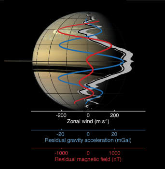
Figure 1: The three measurements used in this study to calculate the Saturnian flow structure. The cloud-level wind (García-Melendo et al., 2011) adjusted with the recently estimated rotation period of 10h 34m (Helled et al., 2015; Mankovich et al., 2019) (black) and a range of winds calculated for rotation periods between 10h 32m (Read et al., 2009) and 10h 39m (Smith et al., 1982) (white shading). The residual gravity field at the planet’s surface $R_{S}$ (blue) based on the dynamical contribution to gravity harmonics $J_{3}$ and $J_{5}$ to $J_{10}$ (Iess et al., 2019; Galanti et al., 2019). The residual radial magnetic field at $0.875R_{S}$ (red) based on the measured Gauss coefficients $g_{4}^{0}$ to $g_{11}^{0}$ (Dougherty et al., 2018; Cao et al., 2020). All values composing the gravity and magnetic fields appear in Table 1. Measurements are shown on top of a Saturn picture taken during the Cassini mission (NASA/JPL-Caltech).

Both missions have also measured at an unprecedented accuracy the magnetic fields of both planets, which differ dramatically between the two planets. On Jupiter, the field has a complex latitudinal and longitudinal structure (Connerney et al., 2018), a characteristic that might be exploited to constrain the flow structure using magnetic secular variations (Moore et al., 2019; Duer et al., 2019). Conversely, the magnetic field on Saturn is extremely axisymmetric (Dougherty et al., 2018; Cao et al., 2020), with latitudinal variability reflecting not only low-order harmonics but also the contribution from higher harmonics (Figure 1, red), which may be related to the structure of the flow below the cloud-level (Gastine et al., 2014; Cao and Stevenson, 2017).

On both planets, the magnetic field measurements provide valuable information that can potentially be used to further constrain the structure of the zonal winds below the cloud-level. Here we report, for the first time, on the well-confined structure of the flow field of Saturn, calculated based on the measured cloud-level wind and both the gravity and magnetic measurements. We then extend our analysis to include the structure of Jupiter’s flow field, using both the measured gravity field and the estimated secular variations of the measured magnetic field.

2 Methods

2.1 The thermal wind balance

Large-scale flows on rapidly rotating planets have a direct relation to density anomalies and, therefore, affect the gravity field if the flows are deep enough (i.e., involve a large mass) (Hubbard, 1999; Kaspi et al., 2010). Such a flow is governed by a geostrophic balance between the anomalous pressure gradient and the Coriolis force (Pedlosky, 1987; Kaspi et al., 2009). Given that on Saturn and Jupiter the flow is predominantly zonally symmetric and assuming sphericity (Galanti et al., 2017b), the resulting vorticity dynamical balance is between the flow gradient in the direction parallel to the axis of rotation and the meridional gradient of density perturbations, known at thermal wind (TW) balance, given by

$$2\Omega r\frac{\partial}{\partial z}\left(\rho_{0}u\right)=g_{0}\frac{\partial\rho^{\prime}}{\partial\theta},$$ (1)

where $u(r,\theta)$ is the zonal zonal flow field, $\Omega$ is the planet’s rotation rate, $\rho_{0}(r)$ and $g_{0}(r)$ are the rigid-body density and gravity fields, $\rho^{\prime}(r,\theta)$ is the anomalous density field, and $z$ is the direction of the axis of rotation. Note that this not the standard atmospheric form of the thermal wind equation (Holton, 1992) as the derivative on the left-hand-side is not in the radial direction, but in the direction of the spin axis (Kaspi et al., 2009). Other effects not included in this balance, such as the anomalous gravity and centrifugal forces induced by the density anomalies (Zhang et al., 2015; Cao and Stevenson, 2017), were shown, for the large scale zonal flows, to have a small effect on the gravity solutions (Galanti et al., 2017b; Kaspi et al., 2018), and therefore are not taken into account here. For the background density $\rho_{0}(r)$ we use the same profiles as were used in the gravity-only studies for Saturn (Galanti et al., 2019) and Jupiter (Kaspi et al., 2018).

The anomalous density field $\rho^{\prime}$ can then be used to calculate the wind-induced gravity harmonics

$$\Delta J_{n}^{{\rm mod}}=-\frac{2\pi}{MR^{n}}\intop_{-\pi/2}^{\pi/2}\cos\theta d\theta\intop_{0}^{R}r{}^{n+2}drP_{n}\left(\sin\theta\right)\rho^{\prime}\left(r,\theta\right)dr,$$ (2)

where $\Delta J_{n}^{{\rm mod}},\,n=2,...,N$ are the coefficients of the wind induced gravity harmonics, $R$ is the planetary radius, and $M$ is the planetary mass. This principle was successfully used to calculate the overall depth of the winds on Jupiter and Saturn using the Juno and Cassini measured gravity field (Kaspi et al., 2018; Iess et al., 2019; Galanti et al., 2019). For the case of Jupiter the calculation was based on the odd gravity harmonics only (Kaspi et al., 2018), and for the case of Saturn also the even harmonics were used, with the expected rigid-body solution subtracted from the measurements (Figure 1, blue, see also Table 1a). These are the solutions we reinvestigate in this study with the new constraints from the magnetic field measurements.

2.2 The mean-field electrodynamic balance

The large scale flow field in Saturn and Jupiter can be also related to a residual magnetic field, induced by the flow in the semi-conducting region where the fluid begins to become conductive (Galanti et al., 2017a; Cao and Stevenson, 2017; Duer et al., 2019). The steady-state balance between the residual magnetic field and the flow, named the mean-field electrodynamics (MFED) balance (Cao and Stevenson, 2017), is

$$\eta_{E}\left(\nabla^{2}-\frac{1}{s^{2}}\right)B+\frac{1}{r}\frac{d\eta_{E}}{dr}\frac{\partial(rB)}{\partial r} = -{\bf B_{0}}\cdot{\bf\nabla}u,$$ (3)

$$\eta_{E}\left(\nabla^{2}-\frac{1}{s^{2}}\right)A = -\alpha B,$$ (4)

where $A(r,\theta,t)$ and $B(r,\theta,t)$ compose the residual magnetic field $\mathbf{B}=\nabla\times(A\hat{e}_{\phi})+B\hat{e}_{\phi}$, $\mathbf{B_{0}}=B_{0}^{r}\hat{e}_{r}+B_{0}^{\theta}\hat{e}_{\theta}$ is the background planetary magnetic field, $\eta_{E}(r)$ is the effective magnetic diffusivity which is inversely proportional to the electrical conductivity $\sigma$, $s=r\sin\theta$ is the distance from the axis of rotation. The function $\alpha(r,\theta)=\alpha_{0}\frac{\eta_{0}}{\eta}{\rm erf}\left(\frac{\theta}{0.005\pi}\right)$ is the dynamo $\alpha$-effect (Cao and Stevenson, 2017), where $\alpha_{0}=10^{-4}\,{\rm m\,s^{-1}}$ is the value at the base of the semi-conducting region (sets by taking the convective velocity there as 1 mm s^-1, and assuming the effective dynamo alpha-effect is 10% of the velocity), and $\eta_{0}$ is the value of the magnetic diffusivity at the base of the semiconducting region.

In this study, we set the electrical conductivity $\sigma$ as an analytical function (Cao and Stevenson, 2017) that reproduces well the measured values (Liu et al., 2008; French et al., 2012). The outer boundary is set where $\sigma=10^{-4}$ S m^-1 ($0.9R_{S}$ for Saturn and $0.98R_{J}$ for Jupiter), and the inner boundary is set where $\sigma=10^{3}$ S m^-1 ($0.845R_{S}$ for Saturn and $0.93R_{J}$ for Jupiter) following Cao and Stevenson (2017). The transition depth is set where $\sigma=0.01$ S m^-1, resulting in $R_{T}=0.875R_{S}$ for Saturn and $R_{T}=0.972R_{J}$ for Jupiter. Note that the transition depth $R_{T}$ might be defined differently (Wicht et al., 2019b), however, this should not affect substantially our results, as long as the conductivity profile remains the same. The model solution is given in terms of the Gauss coefficients $g_{n}^{0}$, similar to the measurements (Table 2). The relation between the Gauss coefficients and the latitude dependent magnetic field in the radial direction (Dougherty et al., 2018), estimated at the transition depth $R_{T}$, is given by

$$B_{r}(\theta)=\sum_{n}(n+1)\left(\frac{R}{R_{T}}\right)^{n+2}g_{n}^{0}P_{n}(\sin\theta).$$ (5)

In the MFED balance it is assumed that the background field is known, and the residual field induced by the flow is small in comparison to the background. Saturn’s measured magnetic field (Dougherty et al., 2018), given in terms of the Gauss coefficients $g_{i}^{0}$ (Table 1), can be separated into the main field, composed of $g_{1}^{0}$ through $g_{3}^{0}$ (used as the background field), and the residual (potentially wind-induced) field, composed of $g_{4}^{0}$ through $g_{11}^{0}$ (Figure 1, red), potentially related to the flow field. The separation into the main and residual fields stems from the significant reduction in the value of $g_{4}^{0}$ compared to $g_{3}^{0}$ (factor of $\sim 25$), and might be attributed to the existence of both a deep dynamo and an outer shallow dynamo (Dougherty et al., 2018). A recent analysis of the Saturn magnetic field (Cao et al., 2020) has pointed to a very similar behavior, with similar conclusions regarding the possibility that the residual field is induced by the flow in the semiconducting region. Nonetheless, it can be argued that in the newer analysis (Cao et al., 2020) (in which $g_{12}^{0}$ to $g_{14}^{0}$ are also calculated), aside from $g_{3}^{0}$, $g_{4}^{0}$ and $g_{6}^{0}$, the higher Gauss coefficients roughly correspond to a straight line in the Lowes-Mauersberger power spectrum (Lowes, 1974), which is an indication that higher harmonics are being generated by the internal dynamo. As we will demonstrate, even if part of the residual magnetic field is not induced by the flow, the results presented here regarding the flow structure in the semiconducting region remain the same. We therefore separate the measured gravity field into the main field composed of $g_{1}^{0}$ to $g_{3}^{0}$, and the residual (potentially wind-induced) field composed of $g_{4}^{0}$ to $g_{11}^{0}$, which we attribute to the flow field. For simplicity we set the background magnetic field $\mathbf{B_{0}}$ as function of $g_{1}^{0}$ only (Equation 5). Including $g_{2}^{0}$ and $g_{3}^{0}$ causes the wind-induced residual magnetic field to have a somewhat smaller amplitude, but does not change qualitatively any of the results reported here.

The constraint on the flow structure used to calculate the decay function in the semiconducting region is taken as the magnitude of the magnetic field $B_{r}$, calculated as the root mean square (RMS) defined between 60^∘S and 60^∘N

$$I=\sqrt{\frac{3}{2\pi}\intop_{-\pi/3}^{\pi/3}B_{r}(\theta)^{2}\,d\theta},$$ (6)

being for the measured field $I=560\,$ nT for Saturn. Using the MFED model we calculate $I$ for different combinations of the two parameters defining the decay function $Q$ in the semiconducting region: $0<f_{M}<1$ and $50\,{\rm km}<H_{M}<800{\rm\,km}$ (see section 2.3).

In the MFED approximation all the non-axisymmetric dynamics are parameterized for (using the dynamo $\alpha$-effect), and only the axisymmetric magnetic field is solved for. This is an excellent assumption for Saturn (Dougherty et al., 2018; García-Melendo et al., 2011), while for Jupiter where the magnetic field was found to exhibit strong east-west variations (Connerney et al., 2018) a method based on magnetic secular variations is more appropriate (Duer et al., 2019; Moore et al., 2019). Another requirement for using the MFED balance is that the magnetic Reynolds number would satisfy $R_{m}(u)<1$ (Cao and Stevenson, 2017). In Appendix D we demonstrate that this is indeed the case for Saturn and Jupiter. Few other factors might affect the MFED solutions: First, the rotation period of Saturn is still not fully known. In this study, we use the more recent estimates of 10h 34m, but other rotation periods cannot be excluded. While it was shown that the rotation period has very little effect on the wind-induced gravity harmonics (Galanti and Kaspi, 2017), it might have an affect on the latitudinal variability of the residual magnetic field. Second, the electrical conductivity used in this study is based on a limited set of measurements and is estimated to have two orders of magnitude uncertainty (Liu et al., 2008). In Appendix C we discuss in detail how this uncertainty affects our solutions. Finally, a more complex $\alpha$-effect with latitudinal dependence, as well as the $\gamma$-effect (Kapyla et al., 2006), are certainly possible and might be calculated from 3D dynamo models, but there is currently uncertainty of what values should be used for Saturn. However, while adding complexity to the solutions, including these parameters should not change the main results reported here.

2.3 Definition of the flow structure

In all variants of flow structure discussed in this study, the same flow field is used to generate both the gravity and the magnetic fields. We start by taking the observed meridional profile of wind at the cloud-level (Figure 1, black line, for Saturn, and Figure 4b, gray line, for Jupiter) and decompose it into the first $N$ Legendre polynomials

$$u^{{\rm obs}}(\theta) = \sum_{i=0}^{N}A_{i}^{{\rm obs}}P_{i}(\sin\theta),$$ (7)

where $A_{i}^{{\rm obs}}$ are the coefficients determining the latitudinal shape of the observed wind, $\theta$ is the latitude, $P_{i}$ are the Legendre polynomials, and $N=99$ is the number of polynomials to be used. Defining a modified cloud-level wind

$$u^{{\rm sol}}(\theta) = \sum_{i=0}^{N}A_{i}^{{\rm sol}}P_{i}(\sin\theta),$$ (8)

where $A_{i}^{{\rm sol}}$ are the modified coefficients, we allow these coefficients to vary during the optimization process while making sure they do not deviate considerably from their observed values. Note that we construct the wind using a very large number of polynomials to allow the wind solution to follow closely the observed wind. The optimization procedure described in Appendix A ensures that the large number of coefficients is well constrained. Next, the modified cloud-level wind $u^{{\rm sol}}(\theta)$ is projected parallel to the axis of rotation (Kaspi et al., 2009) to get the basic non-decaying field $u_{0}(r,\theta)$. This field is then decayed in the radial direction to give

$$u(r,\theta) = u_{{\rm 0}}(r,\theta)Q(r),$$ (9)

where $r$ is the radial direction. The decay function $Q(r)$ is defined as

$$Q(r)=\tanh\left(\frac{r-R_{T}}{\delta H_{T}}\right)\frac{1-f_{M}}{\tanh\left(\frac{R-R_{T}}{\delta H_{T}}\right)}+f_{M},\quad R_{T}<r<R,$$ (10)

$$Q(r)=f_{M}\exp\left(\frac{r-R_{T}}{H_{M}}\right),\quad r\leq R_{T},$$ (11)

where $\delta H_{T}$ is the width of the hyperbolic tangent function, $f_{M}$ is the ratio between the flow strength at the transition depth and the flow at the cloud-level and $H_{M}$ is the decay scale-height in the inner layer. This functional form of the flow’s radial decay allows two distinctly different behaviors in the regions above and below the transition depth $R_{T}$. In the outer region the decay function represents a non-magnetic dynamical effect, with the baroclinic shear being in thermal wind balance (Kaspi et al., 2009), and the free parameter $\delta H_{M}$ allowing a range of decaying profiles, from a gradual decay to a case where the cloud-level winds keep their value almost constant until reaching the transition depth. In the inner region, the exponential decay function is assumed to be a result of the increased electrical conductivity $\sigma$. Based on the choice of the parameters $A_{i}^{{\rm sol}}$$,f_{M}$, $H_{M}$ and $\delta H_{T}$, the flow structure is defined, and can be used to generate both the wind-induced gravity field and the wind-induced magnetic field.

3 Results

The methodology presented above can be more readily applied to Saturn given its highly axisymmetric magnetic field(Dougherty et al., 2018; Cao et al., 2020), while the magnetic field of Jupiter is highly non-axisymmetric (Connerney et al., 2018; Moore et al., 2018), making the usage of the MFED approximation much more challenging. We therefore first investigate the Saturn case with the combined magnetic-gravity analysis, and then discuss the Jupiter case where we substitute the MFED method with insights gained from past measurements of the planet’s magnetic field secular variations (Moore et al., 2019).

3.1 The Saturn case

We start by using the Saturn magnetic field to constrain the flow field. This constraint is set by the magnitude of the measured residual magnetic field, defined here as the root mean square (RMS) of the radial component, $B_{r}$, between 60^∘S and 60^∘N (Figure 1), calculated to be $I=560\,{\rm nT}$ (Equation 6). This is the maximal residual magnetic signature expected from the flow field. By using the MFED balance (section 2.2) and varying the two parameters defining the flow structure in the semiconducting region, $f_{{\rm M}}$ and $H_{{\rm M}}$ (section 2.3), the full range of possible solutions for the wind-induced magnetic field is revealed (Figure 2a). As expected, higher values of $H_{{\rm M}}$ and $f_{{\rm M}}$ (deeper flows) give larger magnetic signatures, with $H_{{\rm M}}$ being the dominant parameter. Since the measured value of 560 nT can be obtained with different combinations of the two parameters (Figure 2a, dashed black contour), the zonal wind’s radial decay in the semiconducting region cannot be determined uniquely. However, different parameter combinations located along the 560 nT contour give very similar solutions for $B_{r}$. For example, the three combinations denoted by the red dots in Figure 2a result in almost identical profiles of $B_{r}$ (Figure 2b, red lines). Most importantly, the shape of the new decay profiles in the semiconducting region (Figure 3a, red lines deeper than the transition depth) are very different from the solution constrained with only the gravity field (Galanti et al., 2019) (dashed black line). The magnetic field measurements imply that the flow must decay sharply at the transition depth. This depth is much shallower than the depth where the gradually decaying gravity-only solution loses most of the wind strength. In addition, due to the magnetic field constraint, in the new solution the long tail does not extend deep into the planet’s interior (gray area).

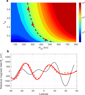
Figure 2: The residual magnetic field induced by the flow structure. (a) The RMS of the residual magnetic field $B_{r}$ at $0.875\,R_{s}$ for a range of flow decay parameters $H_{{\rm M}}$ (km) and $f_{{\rm M}}$. Also shown is the value of the measured field of 560 nT (dashed contour) and three representative combinations of parameters matching the measurements: $H_{{\rm M}}=450,300,250\,{\rm km}$ and $f_{{\rm M}}=0.1,0.45,0.8$, respectively. (b) The resulting latitude-dependent residual magnetic field $B_{r}$ for the three representative combinations: dashed, solid and dashed-doted, respectively. Also shown is the measured field (gray).

3.1.1 A magnetically-restricted solution

Having determined the wind decay functions in the semiconducting region that are consistent with the magnetic field measurements (Table 2), an optimal solution is sought for the wind decay function above the transition depth, such that the associated residual gravity field matches the measured gravity field (Appendix A). Using thermal wind balance (section 2.1), the optimal decay function above the transition depth (Figure 3a, red lines) and the optimal cloud-level wind structure (Figure 3b, red lines) are found, such that the resulting wind-induced gravity field best explains the measured residual gravity field (Figure 1, blue; see also values in Table 1a). Note that since the decay function is optimized only above the transition depth, the solutions still satisfy the magnetic field constraint (Appendix A).

Table 1: (a) The Saturn gravity harmonics $J_{2}$ to $J_{10}$. Shown are the Cassini measurements (Iess et al., 2019), the rigid-body contribution based on an average of ensemble model solutions (Galanti et al., 2019), the dynamical contribution calculated as the difference between the measurements and the rigid-body contribution, the gravity optimized solution (Galanti et al., 2019) based on the gravity measurements only, the new gravity-optimized and MFED-restricted solution, where the MFED restricts the inner part of the decay profile but is not optimized for, and the new gravity and MFED optimized solution where the cloud-level wind is optimized to allow a fit for both gravity and magnetic fields. Note that $J_{2}$ and $J_{4}$ (gray) are not optimized for. (b) The Jupiter gravity harmonics. Shown are the dynamical contributions (measured odds and estimated evens) (Kaspi et al., 2020), the solution based only on the gravity measurements (Kaspi et al., 2018), and the new gravity-optimized and MFED-restricted solution. Note that in the Jupiter case, only $J_{3}$, $J_{5}$, $J_{7}$ and $J_{7}$ (black) are optimized for.

All three optimal solutions are within the measurement uncertainty, with a root mean square error (Equation 15) of 0.34, 0.34 and 0.33 for the main decay profile (solid red), and the two variants (dashed and dotted-dashed), respectively (Table 1a, note that an RMSE of 1 means that the solution harmonics are on average at the measurement error distance from the measurement itself). Note also that the new solutions derived by the magnetic field measurements that dramatically restrict the flow to shallower depth, are not deteriorated compared to the gravity-only solution (with an RMSE of 0.61). In fact, they are better solutions in terms of the RMSE (Table 1a). This improvement is predominantly due to the different decay functions used in the semiconducting region. While in the setup of the gravity-only solution the possible decay function is a combination of synthetic smoother functions, here the physically driven, much sharper decay in the transition depth allows a better fit to the measurements. Moreover, the required modification in the cloud-level wind (Figure 3b, solid red) is marginal with respect to the gravity-only solution, strengthening the robustness of the wind solution with respect to the observed wind. The shape of the new decay function in the outer neutral region implies that, unlike in the gravity-only solution (Figure 3a, dashed black), the winds in the new solution barely decay in the first 7000 km below the cloud-level (i.e., barotropic); only below that depth a decay commences. Only such strong flow in the outer region can generate sufficient mass advection that would be able to explain the gravity measurements.

3.1.2 A fully combined gravity-magnetic solution

The new, depth-confined, solution fits all the relevant gravity harmonics (Table 1a) and the magnitude of the residual magnetic field (Figure 2b, solid red line, and Table 2), but its latitudinal dependence is different from the measured magnetic field. By setting the wind decay profile to the solution already obtained (Figure 3a, solid red line), we perform a full optimization of the cloud-level wind, looking for a solution for which the values of both the induced gravity and magnetic fields are within the uncertainties of the measurements (Appendix B). We obtain an optimal solution (Figure 3b, blue line) with an RMSE of 0.38 for the residual gravity field and an RMSE of 0.99 for the residual magnetic field (Figure 3c, Table 2). Therefore, with the same decay profile, and with only minor modifications to the cloud-level wind, well within the measurement uncertainty (García-Melendo et al., 2011), a flow field is found that can explain the latitudinal dependence of both the gravity and the magnetic fields. In summary, we find that the values of the higher Gauss coefficients pose an upper bound on the wind-induced magnetic field of Saturn. No matter whether the residual field comes from the winds or the deep dynamo, the contributions of the wind in the semiconducting region to the residual field cannot be higher than the measurements, and this strongly constrains the magnitude of the flow in the semiconducting region.

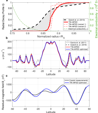
Figure 3: The implication of the magnetic field constraint for Saturn’s flow structure. (a) The new solution for the wind’s radial decay (solid red) together with the gravity-only constrained solution (Galanti et al., 2019) (dashed black). The difference between the solutions is emphasized by the gray area. Also shown are two representative variants of the new solution corresponding to the red dots in Figure. 2a (dashed and dotted-dashed red), the conductivity profile $\sigma\>({\rm S\,m}{}^{-1}$, green), and the transition depth ($0.875\,R_{S}$) separating the outer neutral region and the inner semiconducting region (vertical dashed line). (b) The cloud-level wind profiles. Shown are the observations (García-Melendo et al., 2011) (gray), the new solution with the magnetic field restricting the decay profile (red), the fully optimized new solution with the residual magnetic field optimized in addition to the gravity harmonics (blue), and the gravity-only restricted solution (Galanti et al., 2019) (dashed black). (c) The magnetic field of the fully optimized solution (blue) and the measured residual magnetic field (Dougherty et al., 2018) (gray).

3.1.3 Applicability of the solution

The ability of the MFED balance to constraining the flow field in the semiconducting region should be examined from several aspects. First, a basic requirement for using the MFED balance is that the magnetic Reynolds number, defined as $R_{m}(u)=uH_{\sigma}\sigma\mu_{0}$ ($H_{\sigma}=\sigma/\frac{d\sigma}{dr}$ is the scale height associated with it), would satisfy $R_{m}(u)<1$ (Cao and Stevenson, 2017). We find that $R_{m}(u)$ calculated with the optimal flow solution (Figure 3a), satisfies this condition everywhere (Appendix D). Moreover, the wind-induced residual magnetic field $B_{r}$ can be roughly related to the background field $\mathbf{B_{0}}$ via $B_{r}\sim R_{m}(\alpha)^{{\rm max}}R_{m}(u)^{{\rm max}}\mathbf{|B_{0}|}$, where $R_{m}(\alpha)=\alpha H_{\sigma}\sigma\mu_{0}$ is the magnetic Reynolds number associated with the dynamo $\alpha$-effect (Cao and Stevenson, 2017). Since $R_{m}(\alpha)$ reaches a maximal value of 0.25 (at the lower boundary of the semiconducting region) and $R_{m}(u)<1$ everywhere, the resulting residual magnetic field is always much smaller than the background field (Figure 2b). Second, the MFED balance depends on several parameters that are not strongly constrained. Most importantly, the electrical conductivity $\sigma$ is known only within 2 orders of magnitude (Liu et al., 2008). In order to evaluate the effect of this uncertainty on our solution, we examine two extreme cases, for which $\sigma$ is an order-of-magnitude larger and lower than the mean value used here (Appendix C). In both cases, solutions for the flow field that satisfy both the magnetic and gravity measurements can be found. In the former case, the solution shows an even more pronounced barotropic behavior in the outer layers and an even sharper decay of the winds near the transition depth. In the latter case, the solution exhibits a more gradual wind decay, asymptotically getting closer to (but still far from) the gravity-only solution (Figure 5).

Table 2: The Gauss coefficients composing the magnetic field of Saturn. Shown are the Cassini measurements (Dougherty et al., 2018), the gravity-optimized and MFED-restricted solution, and the optimized model solution corresponding to column 7 in Table 1. Note that in column 3 none of the Gauss coefficients are optimized for, and in column 4, $g_{1}^{0}$, $g_{2}^{0}$ and $g_{3}^{0}$ (gray) are not optimized for.

Moreover, these results also pose a limit on the uncertainty in the conductivity profile, where conductivity that is 2-orders-of-magnitude larger would not allow a physical solution, and that such a limit does not exists for a lower value. Third, the dynamo $\alpha$-effect, parameterizing the action of the small-scale 3D turbulence on the wind induced toroidal magnetic field, is assumed in our study to be only a function of depth, with a sign change at the equator (Cao and Stevenson, 2017). In the framework of the MFED balance, the uncertainty associated with the magnitude of $\alpha$ is equivalent to an uncertainty in $\sigma$. Therefore, its effect on our solutions is similar to the one discussed in the analysis above. Finally, inhomogeneity of $\alpha$ in space or time might also have an effect on the solution, yet these effects are difficult to estimate, and might be compensated by small alterations to the cloud-level wind.

3.2 The Jupiter case

The above results have direct implications for Jupiter, whose gravity measurements were also used to decipher the flow structure (Iess et al., 2018; Kaspi et al., 2018), and whose optimal radial decay based on gravity alone was found to be quite gradual. If the mechanisms governing the flow structure are similar to Saturn’s, constraining Jupiter’s flow with the Juno magnetic field measurements should show a sharp shear at a depth of around 2000 km below the cloud level. As the magnetic field of Jupiter is highly non-axisymmetric (Connerney et al., 2018; Moore et al., 2018), using the MFED approximation is much more challenging, since it involves a non-axisymmetric wind-induced magnetic field, making it more difficult to disentangle this field from the internal field. Recently, using a dynamo model, the effect of different flow structures on the magnetic field in the semiconducting region of Jupiter was estimated, yielding the conclusion that the effect might be measurable by the Juno mission (Wicht et al., 2019b). However, the Lowes spectrum of the higher magnetic harmonics of Jupiter (Connerney et al., 2018), fits roughly a straight line, suggesting that the internal field might play a dominant role in setting their values (Tsang and Jones, 2020). Again, this renders the task of separating the wind-induced magnetic field highly challenging.

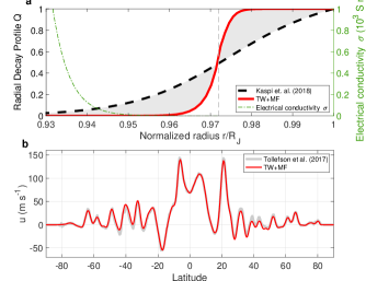
Figure 4: The implication of the magnetic field constraint for Jupiter’s flow structure. (a) The new solution for the wind’s radial decay (solid red) together with the gravity-only constrained solution (Kaspi et al., 2018) (dashed black). The difference between the solutions is emphasized by the gray area. The decay function in the semi-conducting region is defined with $H_{{\rm M}}=200\,{\rm km}$ and $f_{{\rm M}}=0.55$, so that the wind is set to about $2\,{\rm cm\,s^{-1}}$ at $0.93\,R_{J}$ and $0.7\,{\rm m\,s^{-1}}$ at $0.95\,R_{J}$. In the outer region, the decay function is defined with $\delta H_{T}=204$ km. Also shown is the conductivity profile $\sigma\>({\rm S}\,{\rm m}^{-1},$ green) (see Supporting Information for definition), and the transition depth ($0.972\,R_{J}$) separating the outer neutral region and the inner semiconducting region (vertical dashed line). (b) The cloud-level wind profiles. Shown are the observations (Tollefson et al., 2017) (gray) and the new solution with the magnetic field restricting the decay profile (red).

The effect of the wind on Jupiter’s magnetic field might be identified in the magnetic field’s secular variations (Ridley and Holme, 2016; Duer et al., 2019; Moore et al., 2019). Given that a time span of several years of magnetic field measurements is required for calculating the secular variations, an analysis based on the Juno measurements is expected to be available only toward the end of the nominal mission (Bolton et al., 2017). However, we can already use the available studies, and the results of this study, to examine the potential implications for Jupiter. It has been shown, based on the past measurements of Jupiter’s magnetic field and their decadal secular variation (SV), that the magnetic drift at a depth of $0.95\,R_{J}$ is of the order of a few centimeters per second (Moore et al., 2019). The authors conclude that the flow itself can be restricted to the values of the drift rate at $0.93\,R_{J}$, and that Ohmic dissipation considerations limit the flow to an order of 1 m ${\rm s^{-1}}$ in the $0.94$ to $0.95\,R_{J}$ region (Cao and Stevenson, 2017). Since the gravity field is not very sensitive to this region, definitely not to variations of the flow strength below 1 m ${\rm s^{-1}}$, we can confidently choose a decay function that generates such a flow.

Assuming that the mechanism governing the structure of the flow is similar to the one we find in Saturn, a flow structure in the semi-conducting region ($0.95\,R_{J}$ to $0.972\,R_{J}$) can be set such that the above constraint is met (Figure 4a). The magnetic Reynolds number associated with this solution ensures that the wind-induced residual magnetic field is much smaller than the internal field (Appendix D). Similar to the case of Saturn, we search for a solution for the flow structure in the outer layers ($r>0.972\,R_{J}$) such that the measured odd gravity field is explained. By only slightly varying the cloud-level winds (Figure 4b), within the measurement uncertainty (Tollefson et al., 2017), we find a solution for the full decay function (Figure 4a, solid red line). The fit to the gravity field has an RMSE of 0.43, an even better fit to the measurement than the 0.90 achieved with the gravity field alone (Kaspi et al., 2018) (see Table 1b). Importantly, the difference (gray area) between the gravity-only solution and the new solution is substantial, even more than the one found in the Saturn case. The new possible solution for Jupiter is of a structure that is remarkably similar to the new solution for Saturn (Figure 3a, solid red), i.e., almost no decay of the winds from the surface to a depth of around 1800 km, and then a sharp decay over a depth of about 600 km. Similar to the Saturn case, if future studies find the conductivity to be an order-of-magnitude larger than the values used here (Liu et al., 2008), it will strengthen the conclusion regarding the shape of the wind decay. However, an even larger conductivity does not permit a physical solution. Conversely, if the conductivity is found to be much weaker, then the magnetically constrained solution will be more gradual, and closer to the one calculated based only on the gravity field.

4 Discussion and conclusion

The inclusion of the Cassini magnetic measurements as an additional constraint on Saturn’s flow structure below the cloud-level unveils a well-confined flow field that not only can explain the residual magnetic field but also better explains the measured gravity field. Based on constraints from the magnetic secular variation, a similar structure is plausible also in Jupiter. The sharp baroclinic shear of the flow in the semiconducting region, as well as the barotropic structure of the flow from the cloud level down to the transition depth, suggests that the flow interaction with the magnetic field in the semiconducting region (Liu et al., 2008; Cao and Stevenson, 2017) plays an important role in the wind’s decay in the interior of Saturn, Jupiter, and potentially other giant planets (Kaspi et al., 2013; Soyuer et al., 2020). The barotropic nature above this region implies that the observed momentum flux convergence at the cloud-level of Jupiter (Salyk et al., 2006) and Saturn (Del Genio et al., 2007) can drive the flow to great depths, perhaps by the downward control principle (Haynes et al., 1991; Liu and Schneider, 2010), until dissipation due to rising conductivity and interaction with the magnetic field causes its almost abrupt decay. The downward propagation mechanism was shown to be effective also in the presence of a stable layer (Showman et al., 2006), which might also act to decay the flow together with the action of the magnetic field (Christensen et al., 2020). Such a stable layer was recently suggested to be necessary for the case of Jupiter (Debras and Chabrier, 2019).

The results reported here are also in agreement with simulations of the magnetohydrodynamics of gas giants (Heimpel et al., 2005; Gastine and Wicht, 2012; Heimpel et al., 2016; Duarte et al., 2018), in which strong barotropic flows are found above the fully conducting region, and much weaker baroclinic flows inside it. In the barotropic region, the zonal flow is aligned with the axis of rotation according to the Taylor-Proudman theorem (for the compressible case), and horizontal entropy gradients must be small (Jones, 2014). This also implies that the entropy expansion coefficient does not change considerably with depth, as the decay rate of the flow is a product of the entropy gradients and the entropy expansion coefficient (Kaspi et al., 2009). The barotropicity of the neutral region indicates that there is no significant mechanism acting to decay the flow until the semiconducting region is reached. Compared to the gravity-only solution, the restriction of the flow at depth by the magnetic field measurements, requires the flow in the neutral region to be larger, in order for the mass advection to be enough to explain the gravity measurements. We expect the results reported in this study, together with the better understanding of the internal structure of Saturn and Jupiter, to enable better explaining the exact mechanism by which the winds on the gas giants are generated, extended into the planet interior, and finally decay at depth.

Acknowledgments: The authors thank the Juno Interior Working Group for useful discussions. This research was supported by the Israeli Space Agency and the Helen Kimmel Center for Planetary Science at the Weizmann Institute.

Appendix A A magnetically-restricted gravity optimization method

The first set of solutions are performed in the following way. First, the magnetic measurements are used to constrain the decay profile in the semiconducting region. Then the thermal wind model is used to find the optimal decay function in the outer non-conducting region, as well as the optimal cloud-level wind, so that the resulting gravity field explains best the gravity measurements. For the Saturn case, the values used as measurements are the Cassini measurements (Iess et al., 2019) from which the static body harmonics (Galanti et al., 2019) are subtracted

$$J_{n}^{{\rm dyn}}=J_{n}^{{\rm obs}}-J_{n}^{{\rm rigid}},$$ (12)

where $J_{n}^{{\rm obs}}$ are the measured gravity harmonics, and $J_{n}^{{\rm rigid}}$ are the rigid-body solutions taken from the average of an ensemble model solutions (Galanti et al., 2019). Note that $J_{n}^{{\rm rigid}}$ have non-zero values only for the even harmonics. For the Jupiter case, only the odd gravity measurements are used (Iess et al., 2018), and since these are fully wind-induced, there is no need to subtract the solid body contribution (Kaspi et al., 2018) .

The parameters to be optimized, i.e., the parameter defining the flow structure above the semiconducting region and the cloud-level wind latitudinal profile, are defined as a control vector

$$\mathbf{X}_{{\rm C}} = \{\mathbf{X}_{H},\mathbf{X}_{u}\}$$

$$= \left\{\delta H_{T}/h_{{\rm nor}},\left[A_{1}^{{\rm sol}},\cdots,A_{N}^{{\rm sol}}\right]/u_{{\rm nor}}\right\},$$

where $h_{{\bf nor}}=10^{7}$ and $u_{{\bf nor}}=10^{3}$ are the normalization factors for the decay structure and the wind coefficients, respectively. The normalization factors are chosen so that $0<\delta H_{T}/h_{{\rm nor}}<1$ and $-1<A^{{\rm{\rm sol}}}/u_{{\rm nor}}<1$ . Minimizing the difference between the model solution for the gravity field and the measurements, subjected to the uncertainties of the measurements and the need to keep the optimized control parameters regularized to physical values, is achieved with the cost function

$$L_{T} = \mathbf{{\displaystyle\mathbf{\left(J^{m}-\mathbf{J}^{o}\right)}W\left(\mathbf{J^{m}}-\mathbf{J}^{o}\right)^{T}}}$$

$$+ \epsilon_{u}\mathbf{(X_{u}-\mathbf{X}_{o})(X_{u}-\mathbf{X}_{o})^{T}},$$

where for the Saturn case $\mathbf{J^{m}}=\left[J_{3}^{m},J_{5}^{m},J_{6}^{m},J_{7}^{m},J_{8}^{m},J_{9}^{m},J_{10}^{m}\right]$ and $\mathbf{J^{o}}=\left[J_{3}^{{\rm dyn}},J_{5}^{{\rm dyn}},J_{6}^{{\rm dyn}},J_{7}^{{\rm dyn}},J_{8}^{{\rm dyn}},J_{9}^{{\rm dyn}},J_{10}^{{\rm dyn}}\right]$ are the calculated and measured gravity harmonics, respectively, ${\bf W}$ are the uncertainties in the gravity measurements, $\mathbf{X}_{{\rm o}}=\left[A_{1}^{{\rm obs}},\cdots,A_{99}^{{\rm obs}}\right]/u_{{\rm nor}}$ are the observed wind profile parameters and $\epsilon_{u}=5\times 10^{8}$ is the weight given to the regularization of the wind solution to the observed one. For the Jupiter case, $\mathbf{J^{m}}=\left[J_{3}^{m},J_{5}^{m},J_{7}^{m},J_{9}^{m}\right]$ and $\mathbf{J^{o}}=\left[J_{3}^{{\rm dyn}},J_{5}^{{\rm dyn}},J_{7}^{{\rm dyn}},J_{9}^{{\rm dyn}}\right]$. The cost function is composed of two terms, the first is the difference between the measured and calculated gravity harmonics, and the second assures that the wind solution does not vary too far from the observed one at cloud-level. Given the value of $\epsilon_{U}$ and the large number of coefficients defining the wind latitudinal profile, the regularization of the wind is very strong, thus ensuring that deviations from the observed cloud-level wind are allowed only if they result in a significantly lower value of the cost function. Given an initial guess for $\overrightarrow{\mathbf{X}_{{\rm C}}}$, a minimal value of $L$ is searched for using the Matlab function ’fmincon’ and taking advantage of the cost-function gradient that is calculated with the adjoint of the dynamical model Galanti and Kaspi (2016). Finally, the round mean square error (RMSE) we discuss in Table 1 is calculated by

$${\rm RMSE}{}_{{\rm gravity}}=\frac{1}{7}\sum_{N}W_{nn}\left(J_{n}^{m}-J_{n}^{o}\right)^{2},$$ (15)

where $n=3,5,6,7,8,9$ and 10, and $N=7$, for Saturn, and $n=3,5,7$ and 9, and $N=4$, for Jupiter.

Appendix B A combined magnetic-gravity optimization method

The solution for the fully optimized Saturn case is obtained in the following way. The overall decay function is fixed to the function obtained in the gravity optimization, and in the optimization process we look for further modifications in the cloud-level wind so that in addition to the residual measured gravity field explained by the thermal model, the residual magnetic field is also explained by the MFED solution. The MFED model solution is compared to the measured field by minimizing, in addition to $L_{T}$, the cost function

$$L_{M}=\epsilon_{M}\sum_{n=4}^{11}\frac{1}{\left(e_{n}\right)^{2}}\left(\tilde{g}_{n}^{0}-g_{n}^{0}\right)^{2},$$ (16)

where $\tilde{g}_{n}^{0}$ are the MFED model solutions, $e_{n}$ are the measurements errors (Table 1), and $\epsilon_{M}=10^{5}$ is the weight given the cost function. Note that we take into account only the Gauss coefficients $g_{4}^{0}$ to $g_{11}^{0}$ that compose the residual magnetic field. The overall cost function to be optimized is then

$$L=L_{T}+L_{M},$$

and the control vector is now

$$\mathbf{X}_{{\rm C}} = \{\mathbf{X}_{u}\}=\left\{\left[A_{1}^{{\rm sol}},\cdots,A_{N}^{{\rm sol}}\right]/u_{{\rm nor}}\right\},$$ (17)

so that only the parameters composing the cloud-level wind are optimized. The optimization is done jointly. In each iteration the temporal solution for the flow structure is used to generate the gravity harmonics with the thermal wind model and the magnetic coefficients with the MFED model. Then, the cost function $L$ is calculated and a modified cloud-level wind is calculated using Matlab ’fmincon’. Finally, the round mean square error (RMSE) we discuss in Table 2 is calculated by

$${\rm RMSE}{}_{{\rm magnetic}}=\frac{1}{8}\sum_{n=4}^{11}\frac{1}{\left(e_{n}\right)^{2}}\left(\tilde{g}_{n}^{0}-g_{n}^{0}\right)^{2},$$ (18)

where $\tilde{g}_{n}^{0}$ is the model solution.

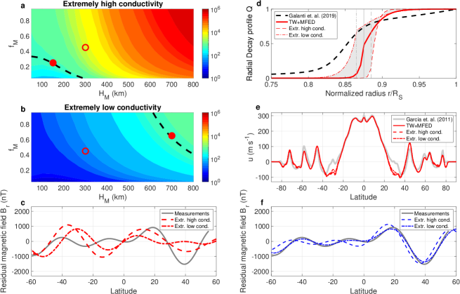
Figure 5: The effect of the uncertainty in the conductivity on the structure of the flow. (a) Similar to Figure 2a, but for a case of extremely high conductivity. The parameter ($H_{M}=150,\,f_{M}=0.25$) result in a wind induced residual magnetic field fitting the measurements (full red circle), indicating a very low winds in the conductive region. (b) Same as (a) but for a case of extremely low conductivity. The parameters $H_{M}=700,\,f_{M}=0.65$ (full red circle), needed for a fit to the measurements, represent a stronger and deep winds in the conductive region. (c) The resulting residual magnetic fields corresponding to the radial flow profiles chosen (full red circles in (a) and (b)). (d) the solutions for the full radial profiles of the extreme cases (red dashed and dashed-dotted), that allow the fitting the gravity field as well. Also shown are the solution from the main text (solid red), and the gravity only (Galanti et al., 2019) solution (black). Note that the transition depth $R_{T}$ is different for each case, denoting the depth where $\sigma=10^{-2}\,{\rm S\,m^{-1}}.$ (e) The cloud-level wind solutions for the two extreme cases. (f) The optimal solution of the residual magnetic field for the two extreme cases (blue dashed and dashed-dotted).

Appendix C Uncertainties in the MFED model

The electrical conductivity $\sigma$ (see section 2), essential to the determination of the wind-induced magnetic field, is known within two order of magnitude in both Jupiter and Saturn (Liu et al., 2008; Wicht et al., 2019b), and therefore the effect of its uncertainty on the radial profile (Figure 3) should be evaluated. While the uncertainty in the electrical conductivity is indeed very large, its effect on the wind-induced magnetic field is less dramatic, due to the exponential nature of the its dependence on depth. To illustrate this we examine two extreme scenarios discussed in the literature (Liu et al., 2008): one in which the conductivity is an order of magnitude larger and one in which it is an order of magnitude lower than the mean value. The results are presented in Figure 5. In both cases, a radial profile of the flow in the semiconducting region can be found (Figure 5a,b) such that the magnitude of the induced residual magnetic field is similar to the measured one (Figure 5c). Next, in both cases, a radial profile in the outer region can be found such that the gravity measurements are also explained (Figure 5d), with a modified cloud-level wind that is very similar to the solution with regular conductivity (Figure 5e). The RMSE for the high and low extreme cases are 0.70 and 0.34, respectively. Note that in the case with the extreme low conductivity, the gravity is slightly easier to match than the standard case. Finally, a fully optimized solution that can explain both the gravity and magnetic measurements can be found for both extreme cases. The gravity RMSE are now 0.92 and 0.30 for the high and low cases, respectively. The magnetic RMSE are now 1.90 and 0.47. Note that, similar to the solutions without fitting the magnetic field details, it is easier to fit the magnetic field latitudinal structure with the extreme low conductivity and somewhat more difficult with the extremely high values. The solutions for both extreme cases show a similar behavior in the outer region where the flow is found to be is mostly barotropic. They also show a similar behavior in having no tail in deep layers. The shift in the depth of the winds between the two extreme cases (gray region in Figure 5d) is about 1000 km, and both solutions are distinctively different from the gravity-only (Galanti et al., 2019) solution (dashed black). With that, it is evident that the stronger electrical conductivity results in a sharper decay of the winds, and the weaker conductivity results in a more moderate decay that is closer to the shape obtained when fitting the gravity field only.

Based on the above analysis, we can also discuss even more extremes values of the conductivity. The solution with the order of magnitude higher conductivity is already not as good as the regular one (Figure 5f), and more importantly, further increase in the value will push the shape of the decay function in the semiconducting region to be unphysical. This is evident in Figure 5a, where the values defining the decay function, $H_{M}$ and $f_{M}$, are already quite close to zero for the extreme case (solid red dot). Solving the model with another order of magnitude larger conductivity makes the problem unsolvable. In addition, the high conductivity already pushes the winds to be completely barotropic in the outer region (Figure 5d, dashed red line). As we discuss in section 3.1.1, this is necessary in order to explain the gravity harmonics, since this extreme decay function involves less mass (weaker winds) in the semiconducting zone, and therefore more mass (stronger winds) has to be included in the outer region. Pushing the decay depth even closer to the surface, will not allow a fit to the gravity measurements. As for the extremely weak conductivity, there our model does not pose any constraint. The weaker the conductivity (or $\alpha$-effect) is, the more the solution becomes similar to the gravity only solution, and there can always be a larger value for $H_{M}$ to define the exponential decay in the semiconducting region.

Another source for uncertainty is the dynamo $\alpha$-effect of which the latitudinal dependence is not well known (Cao and Stevenson, 2017). However, modifying the latitudinal dependency of the $\alpha$-effect, as well as adding the $\gamma$-effect (Kapyla et al., 2006), might add complexity to the solution but would not change the main results (Cao and Stevenson, 2017; Galanti et al., 2017a). First, the magnitude of $\alpha$ would not be significantly different. Second, while the latitude dependency of the solution will change, but as demonstrated here, with minor modification of the cloud-level wind, the details of the measurements can be explained by the model solution. Finally, under the assumptions taken in the MFED of small scale turbulence in the entire semiconducting region, modifying the overall magnitude of the dynamo $\alpha$-effect is equivalent in general to changing the value of the conductivity (see equation 4), therefore the exploration above should suffice to account for that uncertainty. With that, it should be noted that a strongly stratified layer would disconnect the region below it from the winds above, and render the $\alpha$-effect to be smaller. However, such a stable layer, if existed, is expected to be in deeper layers (Debras and Chabrier, 2019).

Appendix D Estimates for the magnetic Reynolds number

A basic requirement for using the MFED balance is that the magnetic Reynolds number would satisfy $R_{m}(u)<1$ (Cao and Stevenson, 2017) (it is defined as $R_{m}(u)=uH_{\sigma}\sigma\mu_{0}$, where $u(r,\theta)$ is the flow velocity, $\sigma$ is the electrical conductivity and $H_{\sigma}=\sigma/\frac{d\sigma}{dr}$ is the scale height associated with it). In Figure 6a we show $R_{m}(u)$ calculated with the Saturn’s optimal flow solution (Figure 3a), where the maximal value in the semiconducting region is 0.98, thus the condition is satisfied. Note that $R_{m}(u)$ becomes extremely small close to the lower boundary because the modeled flow goes to zero there, while in reality the flow strengthens, and so $R_{m}(u)$ might be higher there. This has practically no effect on our results and conclusion since the gravity harmonics are not sensitive to $O$(1) m s^-1 variations at these depths. Moreover, the wind-induced residual magnetic field $B_{r}$ can be roughly related to the background field $\mathbf{B_{0}}$ via $B_{r}\sim R_{m}(\alpha)^{{\rm max}}R_{m}(u)^{{\rm max}}\mathbf{|B_{0}|}$, where $R_{m}(\alpha)=\alpha H_{\sigma}\sigma\mu_{0}$ is the magnetic Reynolds number associated with the dynamo $\alpha$-effect (Cao and Stevenson, 2017). Since $R_{m}(\alpha)$ reaches a maximal value of 0.25 (at the lower boundary of the semiconducting region) and $R_{m}(u)<1$ everywhere, the resulting residual magnetic field is ensured to be much smaller than the background field (Figure 2b). With that, the $R_{m}(u)$ associated with our solution is close to 1 in some regions indicates that the actual flow in the semiconducting region, especially in its outer part, might be weaker than our solution.

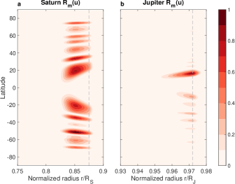
Figure 6: The magnetic Reynolds number $R_{m}(u)$ for the Saturn (a) and Jupiter (b) solutions, in the semiconducting region. In the Saturn case $R_{m}(u)^{max}=0.98$ and in the Jupiter case $R_{m}(u)^{max}=0.88$. Thus, in both cases the basic requirement that enables using the MFED balance, $R_{m}(u)<1$, is met.

The measured residual magnetic field will then not be solely due to the winds (see above discussion). In such a case, the decay of the wind around the 7,000 km depth would be even sharper. A similar analysis was performed with Jupiter’s optimal solution (Figure 4a). The magnetic Reynolds number associated with this solution (Figure 6b) has a maximum value of 0.88 in that region, and is less than 0.1 in most of the domain, thus ensuring that the wind-induced residual magnetic field will be much smaller than the internal field. Note that other methods for estimating $R_{m}(u)$ might be used (Wicht et al., 2019a), but this should not affect substantially the results shown here.

References

- Atkinson et al. (1996) Atkinson, D. H., J. B. Pollack, and A. Seiff, Galileo doppler measurements of the deep zonal winds at Jupiter, Science, 272, 842–843, 1996.
- Bolton et al. (2017) Bolton, S. J., et al., Jupiter’s interior and deep atmosphere: The initial pole-to-pole passes with the Juno spacecraft, Science, 356, 821–825, doi:10.1126/science.aal2108, 2017.
- Cao and Stevenson (2017) Cao, H., and D. J. Stevenson, Zonal flow magnetic field interaction in the semi-conducting region of giant planets, Icarus, 296, 59–72, doi:10.1016/j.icarus.2017.05.015, 2017.
- Cao and Stevenson (2017) Cao, H., and D. J. Stevenson, Gravity and zonal flows of giant planets: From the Euler equation to the thermal wind equation, J. Geophys. Res. (Planets), 122, 686–700, doi:10.1002/2017JE005272, 2017.
- Cao et al. (2020) Cao, H., M. K. Dougherty, G. J. Hunt, G. Provan, S. W. H. Cowley, E. J. Bunce, S. Kellock, and D. J. Stevenson, The landscape of Saturn’s internal magnetic field from the Cassini Grand Finale, Icarus, 344, 113541, doi:10.1016/j.icarus.2019.113541, 2020.
- Christensen et al. (2020) Christensen, U. R., J. Wicht, and W. Dietrich, Mechanisms for Limiting the Depth of Zonal Winds in the Gas Giant Planets, Astrophys. J., 890(1), 61, doi:10.3847/1538-4357/ab698c, 2020.
- Connerney et al. (2018) Connerney, J. E. P., et al., A new model of Jupiter’s magnetic field from Juno’s first nine orbits, Geophys. Res. Lett., 45(6), 2590–2596, doi:10.1002/2018GL077312, 2018.
- Debras and Chabrier (2019) Debras, F., and G. Chabrier, New models of Jupiter in the context of Juno and Galileo, Astrophys. J., 872, 100–, doi:10.3847/1538-4357/aaff65, 2019.
- Del Genio et al. (2007) Del Genio, A. D., J. M. Barbara, J. Ferrier, A. P. Ingersoll, R. A. West, A. R. Vasavada, J. Spitale, and C. C. Porco, Saturn eddy momentum fluxes and convection: First estimates from Cassini images, Icarus, 189(2), 479–492, doi:10.1016/j.icarus.2007.02.013, 2007.
- Dougherty et al. (2018) Dougherty, M. K., et al., Saturn’s magnetic field revealed by the Cassini Grand Finale, Science, 362(6410), aat5434, doi:10.1126/science.aat5434, 2018.
- Duarte et al. (2018) Duarte, L. D. V., J. Wicht, and T. Gastine, Physical conditions for Jupiter-like dynamo models, Icarus, 299, 206–221, doi:10.1016/j.icarus.2017.07.016, 2018.
- Duer et al. (2019) Duer, K., E. Galanti, and Y. Kaspi, Analysis of Jupiter’s deep jets combining Juno gravity and time-varying magnetic field measurements, Astrophys. J. Let., 879(2), L22, doi:10.3847/2041-8213/ab288e, 2019.
- Duer et al. (2020) Duer, K., E. Galanti, and Y. Kaspi, The Range of Jupiter’s Flow Structures that Fit the Juno Asymmetric Gravity Measurements, J. Geophys. Res. (Planets), 125(8), e06292, doi:10.1029/2019JE006292, 2020.
- Fletcher et al. (2020) Fletcher, L. N., et al., Jupiter’s Equatorial Plumes and Hot Spots: Spectral Mapping from Gemini/TEXES and Juno/MWR, J. Geophys. Res. (Planets), 125(8), e06399, doi:10.1029/2020JE006399, 2020.
- French et al. (2012) French, M., A. Becker, W. Lorenzen, N. Nettelmann, M. Bethkenhagen, J. Wicht, and R. Redmer, Ab initio simulations for material properties along the Jupiter adiabat, Astrophys. J. Sup., 202(1), 5, doi:10.1088/0067-0049/202/1/5, 2012.
- Galanti and Kaspi (2016) Galanti, E., and Y. Kaspi, An Adjoint-based Method for the Inversion of the Juno and Cassini Gravity Measurements into Wind Fields, Astrophys. J., 820(2), 91, doi:10.3847/0004-637X/820/2/91, 2016.
- Galanti and Kaspi (2017) Galanti, E., and Y. Kaspi, Prediction for the Flow-induced Gravity Field of Saturn: Implications for Cassini’s Grand Finale, Astrophys. J. Let., 843(2), L25, doi:10.3847/2041-8213/aa7aec, 2017.
- Galanti et al. (2017a) Galanti, E., H. Cao, and Y. Kaspi, Constraining Jupiter’s internal flows using Juno magnetic and gravity measurements, Geophys. Res. Lett., 44(16), 8173–8181, doi:10.1002/2017GL074903, 2017a.
- Galanti et al. (2017b) Galanti, E., Y. Kaspi, and E. Tziperman, A full, self-consistent treatment of thermal wind balance on oblate fluid planets, J. Fluid Mech., 810, 175–195, doi:10.1017/jfm.2016.687, 2017b.
- Galanti et al. (2019) Galanti, E., Y. Kaspi, Y. Miguel, T. Guillot, D. Durante, P. Racioppa, and L. Iess, Saturn’s deep atmospheric flows revealed by the Cassini grand finale gravity measurements, Geophys. Res. Lett., 46(2), 616–624, doi:10.1029/2018GL078087, 2019.
- García-Melendo et al. (2011) García-Melendo, E., S. Pérez-Hoyos, A. Sánchez-Lavega, and R. Hueso, Saturn’s zonal wind profile in 2004-2009 from Cassini ISS images and its long-term variability, Icarus, 215(1), 62–74, doi:10.1016/j.icarus.2011.07.005, 2011.
- Gastine and Wicht (2012) Gastine, T., and J. Wicht, Effects of compressibility on driving zonal flow in gas giants, Icarus, 219, 428–442, doi:10.1016/j.icarus.2012.03.018, 2012.
- Gastine et al. (2014) Gastine, T., J. Wicht, L. D. V. Duarte, M. Heimpel, and A. Becker, Explaining Jupiter’s magnetic field and equatorial jet dynamics, Geophys. Res. Lett., 41, 5410–5419, doi:10.1002/2014GL060814, 2014.
- Haynes et al. (1991) Haynes, P. H., M. E. McIntyre, T. G. Shepherd, C. J. Marks, and K. P. Shine, On the ‘Downward Control’ of Extratropical Diabatic Circulations by Eddy-Induced Mean Zonal Forces., J. Atmos. Sci., 48(4), 651–680, doi:10.1175/1520-0469(1991)048<0651:OTCOED>2.0.CO;2, 1991.
- Heimpel et al. (2005) Heimpel, M., J. Aurnou, and J. Wicht, Simulation of equatorial and high-latitude jets on Jupiter in a deep convection model, Nature, 438(7065), 193–196, doi:10.1038/nature04208, 2005.
- Heimpel et al. (2016) Heimpel, M., T. Gastine, and J. Wicht, Simulation of deep-seated zonal jets and shallow vortices in gas giant atmospheres, Nature Geoscience, 9, 19–23, doi:10.1038/ngeo2601, 2016.
- Helled et al. (2015) Helled, R., E. Galanti, and Y. Kaspi, Saturn’s fast spin determined from its gravitational field and oblateness, Nature, 520(7546), 202–204, doi:10.1038/nature14278, 2015.
- Holton (1992) Holton, J. R., An Introduction to Dynamic Meteorology, third ed., 511 pp., Academic Press, 1992.
- Hubbard (1999) Hubbard, W. B., Note: Gravitational signature of Jupiter’s deep zonal flows, Icarus, 137, 357–359, doi:10.1006/icar.1998.6064, 1999.
- Iess et al. (2018) Iess, L., et al., Measurement of Jupiter’s asymmetric gravity field, Nature, 555, 220–222, doi:10.1038/nature25776, 2018.
- Iess et al. (2019) Iess, L., et al., Measurement and implications of Saturn’s gravity field and ring mass, Science, 364, 1052–, 2019.
- Jones (2014) Jones, C. A., A dynamo model of Jupiter’s magnetic field, Icarus, 241, 148–159, doi:10.1016/j.icarus.2014.06.020, 2014.
- Kapyla et al. (2006) Kapyla, P. J., M. J. Korpi, M. Ossendrijver, and M. Stix, Magnetoconvection and dynamo coefficients - iii. -effect and magnetic pumping in the rapid rotation regime, Astron. and Astrophys., 455(2), 401–412, doi:10.1051/0004-6361:20064972, 2006.
- Kaspi (2013) Kaspi, Y., Inferring the depth of the zonal jets on Jupiter and Saturn from odd gravity harmonics, Geophys. Res. Lett., 40, 676–680, doi:10.1029/2009GL041385, 2013.
- Kaspi et al. (2009) Kaspi, Y., G. R. Flierl, and A. P. Showman, The deep wind structure of the giant planets: Results from an anelastic general circulation model, Icarus, 202(2), 525–542, doi:10.1016/j.icarus.2009.03.026, 2009.
- Kaspi et al. (2010) Kaspi, Y., W. B. Hubbard, A. P. Showman, and G. R. Flierl, Gravitational signature of Jupiter’s internal dynamics, Geophys. Res. Lett., 37, L01,204, doi:10.1029/2009GL041385, 2010.
- Kaspi et al. (2013) Kaspi, Y., A. P. Showman, W. B. Hubbard, O. Aharonson, and R. Helled, Atmospheric confinement of jet-streams on Uranus and Neptune, Nature, 497, 344–347, doi:10.1029/2009GL041385, 2013.
- Kaspi et al. (2020) Kaspi, Y., E. Galanti, A. P. Showman, D. J. Stevenson, T. Guillot, L. Iess, and S. J. Bolton, Comparison of the Deep Atmospheric Dynamics of Jupiter and Saturn in Light of the Juno and Cassini Gravity Measurements, Space Sci. Rev., 216(5), 84, doi:10.1007/s11214-020-00705-7, 2020.
- Kaspi et al. (2018) Kaspi, Y., et al., Jupiter’s atmospheric jet streams extend thousands of kilometres deep, Nature, 555, 223–226, doi:10.1038/nature25793, 2018.
- Kong et al. (2018) Kong, D., K. Zhang, G. Schubert, and J. D. Anderson, Origin of Jupiter’s cloud-level zonal winds remains a puzzle even after Juno, Proc. Natl. Acad. Sci. U.S.A., 115(34), 8499–8504, doi:10.1073/pnas.1805927115, 2018.
- Liu and Schneider (2010) Liu, J., and T. Schneider, Mechanisms of Jet Formation on the Giant Planets, Journal of Atmospheric Sciences, 67(11), 3652–3672, doi:10.1175/2010JAS3492.1, 2010.
- Liu et al. (2008) Liu, J., P. M. Goldreich, and D. J. Stevenson, Constraints on deep-seated zonal winds inside Jupiter and Saturn, Icarus, 196, 653–664, doi:10.1016/j.icarus.2007.11.036, 2008.
- Lowes (1974) Lowes, F. J., Spatial Power Spectrum of the Main Geomagnetic Field, and Extrapolation to the Core, Geophysical Journal International, 36(3), 717–730, doi:10.1111/j.1365-246X.1974.tb00622.x, 1974.
- Mankovich et al. (2019) Mankovich, C., M. S. Marley, J. J. Fortney, and N. Movshovitz, Cassini ring seismology as a probe of Saturn’s interior. I. rigid rotation, Astrophys. J., 871, 1, doi:10.3847/1538-4357/aaf798, 2019.
- Moore et al. (2018) Moore, K., et al., A complex Jovian dynamo from the hemispheric dichotomy of Jupiter’s field, Nature, 561, 76–78, 2018.
- Moore et al. (2019) Moore, K. M., H. Cao, J. Bloxham, D. J. Stevenson, J. E. P. Connerney, and S. J. Bolton, Time variation of Jupiter’s internal magnetic field consistent with zonal wind advection, Nature Astronomy, 3, 730–735, doi:10.1038/s41550-019-0772-5, 2019.
- Pedlosky (1987) Pedlosky, J., Geophysical Fluid Dynamics, pp. 710. Springer-Verlag, 1987.
- Porco et al. (2003) Porco, C. C., et al., Cassini Imaging of Jupiter’s Atmosphere, Satellites, and Rings, Science, 299(5612), 1541–1547, doi:10.1126/science.1079462, 2003.
- Qin et al. (2020) Qin, S., D. Kong, K. Zhang, G. Schubert, and Y. Huang, Interpreting the Equatorially Antisymmetric Gravitational Field of Saturn Measured by the Cassini Grand Finale, Astrophys. J., 890(1), 26, doi:10.3847/1538-4357/ab6a9a, 2020.
- Read et al. (2009) Read, P. L., T. E. Dowling, and G. Schubert, Saturn’s rotation period from its atmospheric planetary-wave configuration, Nature, 460, 608–610, doi:10.1038/nature08194, 2009.
- Ridley and Holme (2016) Ridley, V. A., and R. Holme, Modeling the Jovian magnetic field and its secular variation using all available magnetic field observations, J. Geophys. Res. (Planets), 121(3), 309–337, doi:10.1002/2015JE004951, 2016.
- Salyk et al. (2006) Salyk, C., A. P. Ingersoll, J. Lorre, A. Vasavada, and A. D. Del Genio, Interaction between eddies and mean flow in Jupiter’s atmosphere: Analysis of Cassini imaging data, Icarus, 185, 430–442, doi:10.1016/j.icarus.2006.08.007, 2006.
- Sánchez-Lavega et al. (2000) Sánchez-Lavega, A., J. F. Rojas, and P. V. Sada, Saturn’s zonal winds at cloud level, Icarus, 147, 405–420, doi:10.1006/icar.2000.6449, 2000.
- Showman et al. (2006) Showman, A. P., P. J. Gierasch, and Y. Lian, Deep zonal winds can result from shallow driving in a giant-planet atmosphere, Icarus, 182, 513–526, doi:10.1016/j.icarus.2006.01.019, 2006.
- Smith et al. (1982) Smith, B. A., et al., A new look at the Saturn system: The Voyager 2 images, Science, 215, 505–537, 1982.
- Soyuer et al. (2020) Soyuer, D., F. Soubiran, and R. Helled, Constraining the depth of the winds on Uranus and Neptune via Ohmic dissipation, MNRAS, 498(1), 621–638, doi:10.1093/mnras/staa2461, 2020.
- Tollefson et al. (2017) Tollefson, J., et al., Changes in Jupiter’s zonal wind profile preceding and during the Juno mission, Icarus, 296, 163–178, 2017.
- Tsang and Jones (2020) Tsang, Y.-K., and C. A. Jones, Characterising Jupiter’s dynamo radius using its magnetic energy spectrum, Earth Planet. Sci. Lett., 530, 115,879, doi:https://doi.org/10.1016/j.epsl.2019.115879, 2020.
- Wicht et al. (2019a) Wicht, J., T. Gastine, and L. D. V. Duarte, Dynamo Action in the Steeply Decaying Conductivity Region of Jupiter-Like Dynamo Models, J. Geophys. Res. (Planets), 124(3), 837–863, doi:10.1029/2018JE005759, 2019a.
- Wicht et al. (2019b) Wicht, J., T. Gastine, L. D. V. Duarte, and W. Dietrich, Dynamo action of the zonal winds in Jupiter, Astron. and Astrophys., 629, A125, doi:10.1051/0004-6361/201935682, 2019b.
- Zhang et al. (2015) Zhang, K., D. Kong, and G. Schubert, Thermal-gravitational Wind Equation for the Wind-induced Gravitational Signature of Giant Gaseous Planets: Mathematical Derivation, Numerical Method, and Illustrative Solutions, Astrophys. J., 806(2), 270, doi:10.1088/0004-637X/806/2/270, 2015.