Abstract

How can neural networks learn to efficiently represent complex and high-dimensional inputs via local plasticity mechanisms? Classical models of representation learning assume that input weights are learned via pairwise Hebbian-like plasticity. Here, we show that pairwise Hebbian-like plasticity only works under unrealistic requirements on neural dynamics and input statistics. To overcome these limitations, we derive from first principles a learning scheme based on voltage-dependent synaptic plasticity rules. Here, inhibition learns to locally balance excitatory input in individual dendritic compartments, and thereby can modulate excitatory synaptic plasticity to learn efficient representations. We demonstrate in simulations that this learning scheme works robustly even for complex, high-dimensional and correlated inputs, and with inhibitory transmission delays, where Hebbian-like plasticity fails. Our results draw a direct connection between dendritic excitatory-inhibitory balance and voltage-dependent synaptic plasticity as observed in vivo, and suggest that both are crucial for representation learning.

Significance

Neurons have to represent an enormous amount of sensory information. In order to represent this information efficiently, neurons have to adapt their connections to the sensory inputs. An unresolved problem is how this learning is possible when neurons fire in a correlated way. Yet, these correlations are ubiquitous in neural spiking, either because sensory input shows correlations, or because perfect decorrelation of neural spiking through inhibition fails due to physiological transmission delays. We derived from first principles that neurons can, nonetheless, learn efficient representations if inhibition modulates synaptic plasticity in individual dendritic compartments. Our work questions pairwise Hebbian plasticity as a paradigm for representation learning, and draws a novel link between representation learning and a dendritic balance of input currents.

Introduction

introduction.sectionintroduction.sectionIntroductionIntroductionintroduction.section Many neural systems have to encode high-dimensional and complex input signals in their activity. It has long been hypothesized that these encodings are highly efficient, that is, neural activity faithfully represents the input while also obeying energy and information constrains [1]. For populations of spiking neurons, such an efficient code requires two central features: first, neural activity in the population has to be coordinated, such that no spike is fired superfluously [2]; second, individual neural activity should represent elementary features in the sensory input signal, which reflect the statistics of the stimuli atick1990towardsolshausen_emergence_1996. How can this coordination and these efficient representations emerge through local plasticity rules?

To coordinate neural spiking, a population has to provide information about the population response locally at each neuron. More specifically, for an efficient encoding, input signals should not be encoded redundantly by different neurons, which in many cases means the population should decorrelate responses, e.g. through lateral inhibition. This decorrelation can be realized by networks with excitatory-inhibitory (E-I) balance [5]. Recently it became clear that spiking networks can find an especially cooperative encoding by learning a tight E-I balance [6]. This gave rise to a novel perspective on inhibitory plasticity [7] and the E-I balance in biological networks dehghani_dynamic_2016haider_neocortical_2006: By learning E-I balance, neural responses to input signals are distributed over the population, which, from an information-theoretic and physiological perspective, renders the code efficient [2].

To efficiently encode high-dimensional input signals, it is additionally important that neural representations are adapted to the statistics of the input. Early studies of recurrent networks showed that such representations can be found through Hebbian-like learning of input weights foldiak1990forminglinsker1992local. With Hebbian learning the repeated occurrence of patterns in the input is associated with postsynaptic activity, causing neurons in the population to become detectors of recurrent elementary features. However, this learning also requires the decorrelation of responses through inhibition. Inhibition indirectly guides the learning process by forcing neurons to fire for distinct features in the input. Recent efforts rigorously formalized this idea for models of spiking neurons in balanced networks [12] and spiking neurons sampling from generative models nessler_bayesian_2013bill_distributed_2015nessler2009stdpkappel_stdp_2014. The great strength of these approaches is that the learning rules can be derived from first principles, and turn out to be similar to spike timing dependent plasticity (STDP) curves that have been measured experimentally.

However, to enable the learning of efficient representations, these models have strict requirements on network dynamics and input. Most crucially, inhibition has to ensure that neural responses are sufficiently decorrelated. In the neural sampling approaches, learning therefore relies on strong winner-take-all dynamics. In the framework of balanced networks, inhibition has to be nearly instantaneous and elementary features in the input have to be uncorrelated. These requirements are likely not met in realistic situations.

We here propose a mechanism that overcomes these limitations and enables spiking networks to learn efficient representations. We suggest that inhibition can directly guide the learning of input weights by learning to locally balance specific inputs on dendrites. The resulting balanced dendritic potentials can be used to incorporate information about the population code into the learning of single input weights. In simulations of spiking neural networks we demonstrate the benefits of this learning scheme over Hebbian-like learning for the efficient encoding of high-dimensional inputs. Hence, we extend the idea that balanced state inhibition provides information about the population code locally, and show that not only can it be used to distribute neural responses over a population, but also for an improved learning of input weights.

Results

results.sectionresults.sectionResultsResultsresults.section

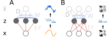
Fig 1: For representation learning, the task is to efficiently encode high dimensional, analog input signals with spikes. A Low dimensional, analog input signals $\mathbf{x}$ can be efficiently encoded by the responses of a large population of spiking neurons $\mathbf{z}$. To that end, neurons couple to the input via weights $F$ and inhibit each other via weights $W$. From the encoding an external observer can decode an approximation $\mathbf{\hat{x}}$ of the original input signal $\mathbf{x}$ via a linear transformation $D$. B In this paper, we ask how high dimensional, analog input signals $\mathbf{x}$ can be efficiently encoded by a small population of spiking neurons. For this more complex task the neurons not only have to translate the continuous input signal into a spiking representation, they also have to compress it by adapting their input weights $F$ to the input statistics.

The goal in this paper is to efficiently encode a continuous high-dimensional input signal by neural spiking. In the following, we will explain how neurons can learn efficient representations of these inputs through local plasticity mechanisms. We will first show how E-I balance can guide neural spiking in order to distribute the encoding over the population. We will then show how E-I balance on the level of dendrites can guide the learning of efficient representations in the input weights.

Background: Efficient encoding by spiking neurons with tight E-I balance

background-efficient-encoding-by-spiking-neurons-through-tight-E-I-balance.subsectionbackground-efficient-encoding-by-spiking-neurons-through-tight-E-I-balance.subsectionBackground: Efficient encoding by spiking neurons with tight E-I balanceBackground: Efficient encoding by spiking neurons with tight E-I balancebackground-efficient-encoding-by-spiking-neurons-through-tight-E-I-balance.subsection

Setup

setup.subsubsectionsetup.subsubsectionSetupSetupsetup.subsubsection

Continuous inputs $\mathbf{x}(t)$ drive a recurrently connected spiking neural network which encodes the inputs through responses $\mathbf{z}(t)$ (Fig 1A). Input weights $F_{ji}$ indicate how strongly excitatory input $x_{i}(t)$ couples to neuron $j$ and lateral inhibitory weights $W_{jk}$ provide negative coupling between the neurons. Neurons in the network encode the inputs by emitting spikes, which then elicit postsynaptic potentials (PSPs) $\mathbf{z}(t)$. The PSPs are modeled as a sum of exponentially decaying depolarizations $z_{j}(t)=\sum_{t_{s}^{j}\leq t-\Delta t}\exp(-\frac{t-\Delta t-t_{s}^{j}}{\tau})$ with decay time $\tau$ for each spike of neuron $j$ at times $t_{s}^{j}$. PSPs arrive after one timestep $\Delta t$, which we interpret as a finite transmission delay of neural communication. Our model is similar to those in previous studies of balanced spiking networks brendel2020learningboerlin2013predictive.

To test whether the input is well encoded, we consider the best linear readout $\mathbf{\hat{x}}(t)=D\mathbf{z}(t)$ of inputs from the neural response and quantify the mean decoder loss

$$\begin{aligned} \mathcal{L}=\frac{1}{N_{x}}\left\langle||\mathbf{x}(t)-\mathbf{\hat{x}}(t)||^{2}\right\rangle_{t}=\frac{1}{N_{x}}\left\langle||\mathbf{x}(t)-D\mathbf{z}(t)||^{2}\right\rangle_{t}\end{aligned},$$ (1)

where $N_{x}$ is the number of inputs. It is important to note that the readout is not part of the network, but only serves as a guidance to define a computational goal that can be reached autonomously via local plasticity rules. Hence learning an efficient code amounts to minimizing $\mathcal{L}$ via local plasticity rules on $F_{ji}$ and $W_{jk}$ given the best decoder $D$.

Spiking neuron model

spiking-neuron-model.subsubsectionspiking-neuron-model.subsubsectionSpiking neuron modelSpiking neuron modelspiking-neuron-model.subsubsection

Spiking neurons are modeled as stochastic leaky integrate-and-fire neurons. Stochastic spiking is important to increase robustness during learning, and allows a direct link to neural sampling and unsupervised learning via expectation-maximization (see SI). A neuron $j$ emits spikes stochastically with a probability that depends on its membrane potential $u_{j}(t)$ according to

$$p_{spike}(u_{j}(t))\propto\exp\left(\frac{u_{j}(t)-T_{j}}{\Delta u}\right).$$ (2)

When the membrane potential approaches the firing threshold $T_{j}$, the firing probability increases exponentially, where $\Delta u$ regulates the stochasticity of spiking. For increasing $\Delta u$ the spike emission becomes increasingly random, whereas for $\Delta u\rightarrow 0$ one recovers the standard leaky integrate-and-fire (LIF) neuron with sharp threshold. The membrane potential itself is modeled as a linear sum of the feed-forward inputs $x_{i}(t)$ and lateral inhibition $z_{k}(t)$, i.e.

$$u_{j}(t)=\underbrace{\textstyle{\sum_{i}}F_{ji}x_{i}(t)}_{\text{excitatory input}}+\underbrace{\textstyle{\sum_{k}}W_{jk}z_{k}(t)}_{\text{lateral inhibition}}.$$ (3)

In order to fix the number of spikes for an efficient code, the average firing rate of each neuron was controlled via the threshold $T_{j}$ (Fig 2C).

Somatic balance enables an efficient encoding for low-dimensional input signals

somatic-balance-enables-an-efficient-encoding.subsubsectionsomatic-balance-enables-an-efficient-encoding.subsubsectionSomatic balance enables an efficient encoding for low-dimensional input signalsSomatic balance enables an efficient encoding for low-dimensional input signalssomatic-balance-enables-an-efficient-encoding.subsubsection

Spiking neurons can implement an efficient encoding for low dimensional input signals by tightly balancing feed-forward inputs and lateral inhibition at the soma [6]. In fact, for one dimensional inputs a tight balance directly implies an efficient encoding. In this case, the inhibitory weights can be rewritten as $W_{jk}=-F_{j}D_{k}$ for fixed input weights $F$ and some decoder $D$. Similarly, the membrane potentials can be written as $u_{j}(t)=F_{j}\left(x(t)-\hat{x}(t)\right)$, with $\hat{x}(t)=\sum_{k}D_{k}z_{k}(t)$. Thus, when the membrane potentials are tightly balanced, i.e. $u_{j}(t)\approx 0$ most of the time, then the two requirements of an efficient code are fulfilled: First, the decoder $D$ is able to accurately reconstruct the input from the network activity. Second, since the neurons are only driven by the coding error $x(t)-\hat{x}(t)$, no superfluous spike is fired that does not improve the encoding.

This motivates that networks can autonomously find an efficient encoding by enforcing a tight balance through local inhibitory plasticity (see SI for derivation)

$$\Delta W_{jk}\propto-z_{k}u_{j}=-z_{k}\left(\textstyle{\sum_{i}}F_{ji}x_{i}+\textstyle{\sum_{l}}W_{jl}z_{l}\right)\quad\text{(somatic balance)}.$$ (4)

Hence, when neuron $k$ is active and the somatic potential of neuron $j$ is out of balance, i.e. $u_{j}(t)\neq 0$, the weight $W_{jk}$ changes to balance $u_{j}(t)$. Note, that all neurons have an autapse that learns to balance their own membrane potentials, which can alternatively be interpreted as an approximate membrane potential reset after spiking. As was shown in [12], tight E-I balance is sufficient to efficiently encode low dimensional input signals (Fig 1A).

Learning efficient representations with plastic input synapses

main-result-efficient-representations-by-spiking-neurons-through-plastic-input-synapses.subsectionmain-result-efficient-representations-by-spiking-neurons-through-plastic-input-synapses.subsectionLearning efficient representations with plastic input synapsesLearning efficient representations with plastic input synapsesmain-result-efficient-representations-by-spiking-neurons-through-plastic-input-synapses.subsection

While the exact choice of input weights $F$ is irrelevant for low dimensional inputs, it becomes increasingly important for high dimensional inputs with complex statistical structure (Fig 1B). It is possible to derive a plasticity rule for input synapses $F_{ji}$ that minimizes the decoder loss $\mathcal{L}$ via gradient descend, which yields

$$\Delta F_{ji}\propto z_{j}(x_{i}-\hat{x}_{i})=z_{j}(x_{i}-\textstyle{\sum_{k}}D_{ik}z_{k}).$$ (5)

Intuitively, this rule drives neuron $j$ to correlate its output $z_{j}$ to input $x_{i}$, except if the population is already encoding it. To extract the latter information, the plasticity rule requires a decoding $\hat{x}_{i}=\sum_{k}D_{ik}z_{k}$, which contains information about the neural code for input $i$ of all other neurons in the population.

We thus conclude that an efficient code relies on information about other neurons in two ways: (i) neurons need to know what is already encoded to avoid redundancy in spiking (dynamics), (ii) plasticity of input connections requires to know what neurons encode about specific inputs to avoid redundancy in representation (learning). While inhibitory weights $W_{jk}$ for efficient spiking dynamics (i) can be learned locally (Eq 4), learning input synapses $F_{ji}$ (ii) is not feasible locally for point neurons, since they lack knowledge about the population code for single inputs $x_{i}$.

In the following, we will introduce the main result of this paper: similarly to efficient spiking through a tight balance of all excitatory and inhibitory inputs at the soma, local learning of efficient representations can be realized by tightly balancing specific excitatory inputs with lateral inhibition. Physiologically, we argue that this corresponds to spatially separated inputs at different dendritic compartments, where dendritic inhibition locally balances the membrane potential. We contrast this local implementation of the correct gradient of the decoder loss with a common local approximation of the gradient, which is necessary for neurons with somatic balance only.

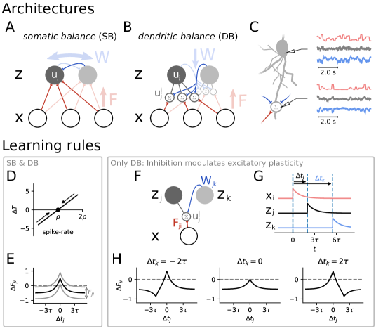
Fig 2: We compare learning in two network models, a classical model of point neurons with somatic balance, and a model with dendritic balance. A In the classical model (SB), neurons (grey circles) with outputs $\mathbf{z}$ receive feed-forward network inputs $\mathbf{x}$ (white circles) and are coupled via lateral inhibition. Inhibitory weights $W$ are adapted to balance excitatory currents at the soma with membrane potential $u_{j}$, which ensures an efficient spike encoding. B In our proposed model (DB), neurons receive inputs at specific dendritic compartments. Inhibition learns to balance input currents locally at the dendrites. This leads to dendritic potentials $u^{i}_{j}$ that are proportional to the coding error for specific inputs, and therefore can be used to learn input weights. C After learning, local excitatory (red) and inhibitory (blue) currents have adapted to tightly balance each other at individual dendrites (bottom). This dendritic balance also results in a somatic balance of inputs (top). Here we show a neuron from a network with 80 neurons coding for natural images. D In both models a rapid compensatory mechanism ensures that every neuron fires with rate $\rho$. If any neuron spikes too rarely, its threshold $T_{j}$ is lowered; if it spikes too often $T_{j}$ is increased. This mechanism allows that the performances of SB and DB can be compared, but is not required for stable network function (see Methods). E For learning input weights in the classical model a Hebbian-like STDP rule increases or decreases weights $F_{ji}$ depending on the time difference between pre- and postsynaptic spikes $\Delta t_{j}$, and the weight $F_{ji}$ itself. If $F_{ji}$ is high or low, this shifts plasticity towards depression or potentiation, respectively. The same learning rule applies to the proposed model, if a neuron does not simultaneously receive any inhibition. F-H Illustration of how inhibition modulates input plasticity in the proposed model for a network of two coding neurons $z_{j}$ (with one dendritic compartment) and $z_{k}$ and one input neuron $x_{i}$. F The excitatory weight $F_{ij}$, as well as the inhibitory weight $W_{jk}^{i}$, attach to the same dendritic potential $u^{i}_{j}$. G We consider the following example where three spikes are fired: $x_{i}$ at $t=0$, $z_{j}$ at $t=\Delta t_{j}$ and $z_{k}$ at $t=\Delta t_{k}$. H The total change in the weight $F_{ji}$ depends not only on the spike-time difference $\Delta t_{j}$ between the input and the postsynaptic neuron, but also on the relative inhibitory spike-time $\Delta t_{k}$. In general, if $z_{j}$ and $z_{k}$ spike close together, $F_{ji}$ will tend to be depressed. All weight-changes were calculated with $F_{ji}=-W_{jk}^{i}=0.5$.

Somatic balance alone requires an approximation for local learning

somatic-balance-alone-requires-a-local-approximation.subsubsectionsomatic-balance-alone-requires-a-local-approximation.subsubsectionSomatic balance alone requires an approximation for local learningSomatic balance alone requires an approximation for local learningsomatic-balance-alone-requires-a-local-approximation.subsubsection

Since somatic balance alone cannot provide information about other neurons at the input synapses, previous approaches used a local approximation to $\Delta F_{ji}$ where only pre- and postsynaptic currents are taken into account (Fig 2E)

$$\Delta F_{ji}\propto z_{j}(x_{i}-F_{ji}z_{j})\quad(\text{Hebbian-like learning}).$$ (6)

We will refer to this setup as somatic balance (SB), because inhibition is mediated by inhibitory connections that balance the somatic potential $u_{j}(t)$.

The above learning rule is exact when simultaneous coding, and thus non-local dependencies during learning, are not present. This is the case when only a single PSP $z_{j}(t)$ is nonzero at a time, e.g. in winner-take-all circuits with extremely strong inhibition [14], or when the PSP is extremely short [13]. The learning rule becomes also approximately exact when neural PSPs $\mathbf{z}(t)$ in the encoding are uncorrelated foldiak1990formingbrendel2020learning. However, these are strong demands on the dynamics of the network which ultimately limit its coding versatility.

Dendritic balance allows local learning of efficient representations

dendritic-balance-allows-local-learning-of-efficient-representations.subsubsectiondendritic-balance-allows-local-learning-of-efficient-representations.subsubsectionDendritic balance allows local learning of efficient representationsDendritic balance allows local learning of efficient representationsdendritic-balance-allows-local-learning-of-efficient-representations.subsubsection

When neural PSPs $\mathbf{z}(t)$ in the population are correlated, learning efficient representations at input synapses requires that information about the population code for this input is available at the synapse. To this end, we introduce local dendritic potentials $u_{j}^{i}$ at synapses $F_{ji}$, and couple neurons $k$ via dendritic inhibitory connections $W_{jk}^{i}$ to these membrane potentials (Fig 2B). The somatic membrane potential is then realized as the linear sum of the local dendritic potentials

$$\begin{gathered}u_{j}(t)=\textstyle{\sum_{i}}u_{j}^{i}(t)\\ u^{i}_{j}(t)=\underbrace{F_{ji}x_{i}(t)}_{\text{excitatory input}}+\underbrace{\textstyle{\sum_{k}}W^{i}_{jk}z_{k}(t)}_{\text{dendritic inhibition}}.\end{gathered}$$ (7)

Note that this amounts only to a refactoring of the equation for the somatic membrane potential and does not change the computational power of the neuron. Given a network using dendritic inhibition with inhibitory weights $W^{i}_{jk}$, a network using somatic inhibition with weights $W_{jk}=\sum_{i}W^{i}_{jk}$ is equivalent. Hence, any improvement in the neural code through dendritic balance is due to an improvement in the learning of feed-forward weights.

The local integration of dendritic inhibition allows to use the same trick as before: by enforcing a tight E-I balance locally, dendritic inhibition will try to cancel the input as well as possible. Thereby, dendritic inhibitory weights $W_{jk}^{i}$ will automatically learn the best possible decoding of the population activity $\mathbf{z}$ to the input $F_{ji}x_{i}$. This leads to a local potential that is proportional to the coding error $u^{i}_{j}=F_{ji}(x_{i}-\hat{x}_{i})$. In terms of synaptic inhibitory plasticity this is realized by

$$\Delta W^{i}_{jk}\propto-z_{k}u^{i}_{j}\quad\text{(dendritic balance)}.$$ (8)

Thus, the dendritic membrane potential $u^{i}_{j}$ can be used to find the correct gradient $\Delta F_{ji}$ from Eq 5 locally

$$\Delta F_{ji}\propto\frac{1}{F_{ji}}z_{j}u^{i}_{j}\quad\text{(learning by errors)}.$$ (9)

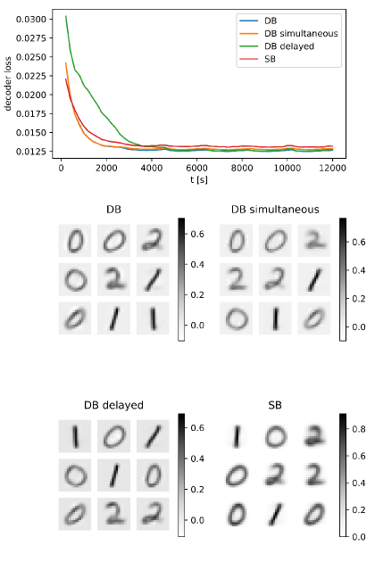
Fig S2: Comparison of the different learning schemes on the MNIST task.

As can be seen, the learning rules for input and inhibitory weights both rely on the local dendritic potential, which they also influence. This enables local inhibition to modulate feed-forward plasticity. However, in our model this also requires the cooperation of the excitatory and inhibitory weights during learning. We propose two different implementations which ensure this cooperation, by learning inhibitory weights on a faster, or on the same timescale as excitatory weights (see SI). We show that these two approaches yield similar results which equal the analytical solution (Eq 5) in performance (see Fig S2,S3).

It is possible to integrate the learning rules which depend on membrane potentials over time and obtain learning rules which depend on the relative spike timings of multiple neurons. If we only consider one input neuron and one coding neuron, learning with dendritic balance and somatic balance yield the same spike timing dependent plasticity rule. This rule is purely symmetric and strengthens the connection when both neurons fire close in time (Fig 2E). However, if the spike of the excitatory input neuron is accompanied by an inhibitory spike in the coding population, the spike timing dependent rule breaks symmetry (Fig 2H). This shows how learning with dendritic balance can take more than pair-wise interactions into account when learning weights to enable the neuron to find its place in the ongoing activity.

Simulation experiments

Simulation-experiments.subsectionSimulation-experiments.subsectionSimulation experimentsSimulation experimentsSimulation-experiments.subsection

To illustrate the differences that arise between the networks using somatic balance (SB) and dendritic balance (DB) during learning, we set up several coding tasks of increasing complexity. In order to facilitate the interpretation of the input features learned by the neurons, we tasked the neural population to code for images. The images were presented as constant input signals over time and faded in between presentations to avoid discontinuities. Learning was performed on-line in an unsupervised fashion and single neurons consistently learned to represent elementary features of the input stimuli. We quantified performance by measuring the decoder loss of this neural code on a separate set of test stimuli with plasticity rules turned off.

Simple stimuli are encoded equally well by networks using somatic or dendritic balance

simple-stimuli-are-encoded-equally-well-by-networks-using-somatic-or-dendritic-balance.subsubsectionsimple-stimuli-are-encoded-equally-well-by-networks-using-somatic-or-dendritic-balance.subsubsectionSimple stimuli are encoded equally well by networks using somatic or dendritic balanceSimple stimuli are encoded equally well by networks using somatic or dendritic balancesimple-stimuli-are-encoded-equally-well-by-networks-using-somatic-or-dendritic-balance.subsubsection

In a first test we performed a comparison on the MNIST dataset of handwritten digits (Fig 3E). We restricted the dataset to the digits 0, 1 and 2, which were encoded by 9 coding neurons. After learning, the input weights of both networks had converged to detect prototypical digits (Fig 3D) and the codes and coding performances were approximately equal (Fig 3C). Since images were rarely encoded by more than one or two neurons (Fig 3A, B), interactions in the population were small and thus the learning rules found similar solutions.

Dendritic balance can disentangle correlated features

dendritic-balance-can-disentangle-weak-correlations.subsubsectiondendritic-balance-can-disentangle-weak-correlations.subsubsectionDendritic balance can disentangle correlated featuresDendritic balance can disentangle correlated featuresdendritic-balance-can-disentangle-weak-correlations.subsubsection

Our theoretical results suggest that DB networks should find a better encoding than SB networks when weak correlations between elementary features are present in the stimuli. To test this, we devised a variation of Földiak’s bar task [10], which is a classic independent component separation task. In the original task neurons encode images of independently occurring but overlapping vertical and horizontal bars. Since the number of neurons is equal to the number of possible bars in the images, each neuron should learn to represent a single bar to enable a good encoding. We kept this basic setup but additionally we introduced between-bar correlations for selected pairs of bars (Fig 4A). We then could vary the correlation strength $p$ between the bars within the pairs to render them easier or harder to separate.

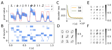
Fig 3: Simple stimuli are encoded equally well by networks using somatic or dendritic balance. In this simulation experiment, networks consisting of 9 coding neurons encoded 16x16 images of digits 0, 1 and 2 from the MNIST dataset. A Input signal $x_{i}$ and decoded signal $\hat{x}_{i}$ for a single pixel $i$ in the center of the image. MNIST digits were presented as constant input signals for $70\,\text{ms}$ and faded for $30\,\text{ms}$ to avoid discontinuities. The decoded signal tracks the input reasonably well given the very limited capacity of the the network. B Spike train of all neurons in the network in response to the input signal in A. C Decoder loss decreases with neural plasticity for both models using either somatic balance (SB), or dendritic balance (DB). Both models have very similar learning speed and final performance. The decoder loss was calculated on a fixed set of test images. In this example, DB is realized by simultaneous learning of input and inhibitory weights (see SI). D Input weights of the 9 coding neurons in the DB network after learning. Every neuron becomes specific for a certain prototypical digit. E Sample of input images from the MNIST dataset. F Reconstructions $\mathbf{\hat{x}}$ of the input images shown in E. The reconstructions presented here are calculated by averaging the decoded signal during input signal presentation over $70\,\text{ms}$. In A,B,D and F we show results of the converged DB network.

The simulation results indeed showed that the performance of SB, but not of DB, deteriorates when elementary features are correlated (Fig 4B). The decoder loss for SB grows for increasing $p$ and reaches its maximum at about $p=0.8$. This is because Hebbian-like learning (as used in SB) correlates a neuron’s activity with the appearance of patterns in the input signal, irrespective of the population activity. The correlation between two bars therefore can lead a neuron which initially is coding for only one of the bars to incorporate also the second bar into its receptive field. Thus, with a certain correlation strength $p$ between bars the receptive fields of neurons start to collapse. For $p>0.8$ the decoder loss decreases, as here the occurrence of specific pairs of bars becomes so likely, that the collapsed representations reflect the statistics of the images again. In contrast, DB enables neurons to communicate which part of the input signal they encode and hence they consistently learn to code for single bars. Accordingly, the decoder loss for DB is smaller than for SB for every correlation strength of bars.

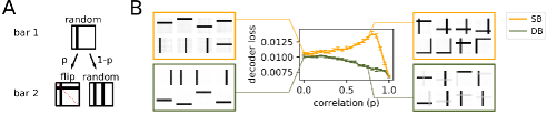
Fig 4: Dendritic balance enables neurons to disentangle feature correlations in the input. In this simulation experiment, 16 neurons code for 8x8 images containing two random out of 16 possible bars. Thus, optimally, every neuron codes for a single bar. A Creation of input images with correlation between features. Two bars are selected in succession and added to the image. With probability $p$ the bars are symmetric around the top-left to bottom-right diagonal axis. With probability $1-p$ the two bars are chosen randomly. B Decoder loss after learning for different correlation strengths. Displayed is the median decoder loss for 50 different realizations for each data point; error-bars denote 95% bootstrap confidence intervals. On the sides, 8 out of all 16 converged input weights are shown for representative networks. When correlations between bars are present, the representations learned by SB overlap, while DB still learns efficient single bar representations.

Dendritic balance improves learning for images of natural scenes

dendritic-balance-improves-learning-for-images-of-natural-scenes.subsubsectiondendritic-balance-improves-learning-for-images-of-natural-scenes.subsubsectionDendritic balance improves learning for images of natural scenesDendritic balance improves learning for images of natural scenesdendritic-balance-improves-learning-for-images-of-natural-scenes.subsubsection

We expected to see a similar difference between SB and DB networks when complex stimuli are to be encoded. In a third experiment we therefore tested the performance of the networks encoding images of natural scenes. We used 8x8 pixel images cut out from a set of pictures of landscapes and vegetation with suitable preprocessing (Fig 5A). To also test whether the amount of compression (number of inputs vs. number of coding neurons) would affect SB and DB networks differently, we varied the number of coding neurons while keeping the population rate fixed at 1000Hz. This way, only the compression, and not also the total number of spikes, has an effect on the performance of the networks.

The simulations showed that complex stimuli can be represented better by DB networks compared to SB networks. This difference becomes larger the higher the compression of the input signal by the network is (Fig 5B). This effect seems to be related to the observations we made in the bar task: Networks with few coding neurons have to learn correlated features, which renders SB less appropriate. We found that SB networks consistently needed about twice as many neurons to achieve a similar coding performance as DB networks.

We also note that the amount of compression affects the strategy neurons resort to in order to encode the images. When the number of coding neurons is bigger than the dimension of the input signal, neurons form Gabor wavelet-like receptive fields. For a smaller number of coding neurons, on the other hand, the neurons develop center surround receptive fields, pooling adjacent input dimensions.

Dendritic balance can cope with long transmission delays

dendritic-balance-can-cope-with-long-transmission-delays.subsubsectiondendritic-balance-can-cope-with-long-transmission-delays.subsubsectionDendritic balance can cope with long transmission delaysDendritic balance can cope with long transmission delaysdendritic-balance-can-cope-with-long-transmission-delays.subsubsection

A central problem for balanced networks is that long transmission delays of inhibition can deteriorate network performance [18]. We found that DB networks are much more robust to longer transmission delays than SB networks. To investigate this, we simulated networks of 200 neurons with a range of time steps $\Delta t$, which we interpret as transmission delays. We varied the delay from $\Delta t=0.1\text{ms}$ to $\Delta t=10\text{ms}$ and observed how the delay affected coding performance for natural images.

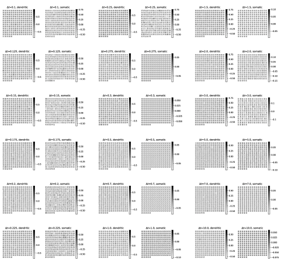
Fig S7: All learned weights for the natural scenes task for different timesteps (Fig 6A).

We found that performance of SB networks drastically broke down to a baseline level when transmission delays became longer than $0.3\text{ms}$ (Fig 6A). All neurons had learned the same feed-forward weights (Fig S7). In contrast, DB networks continued to perform well even for much longer delays. While long delays for DB also lead to a decrease in coding performance, DB prevented the sudden collapse of the population code.

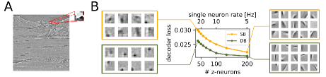
Fig 5: Dendritic balance enables learning of efficient representations of complex, natural stimuli. A Exemplary image from the natural-scenes data-set. We extracted 16x16 pixel images from a set of whitened pictures of natural scenes [4], scaled them down to 8x8 pixels and applied a non-linearity (see SI). B Decoder loss after learning of SB and DB networks featuring varying numbers of coding neurons, while keeping the population rate constant at $1000\,\text{Hz}$. On the sides we show exemplary converged input weights. For a large number of coding neurons (right) both learning schemes yield similar representations, but performance is slightly better for DB. For a small number of neurons (left) DB learns more refined representations with substantially reduced decoder loss as compared to SB. The reason is that for a small number of neurons the learned features are more correlated and consequently are harder to disentangle. Notably, different amounts of neurons result in different coding strategies.

To illustrate the mechanism that caused the breakdown in performance for SB, we also ran simulations of networks learning to code for MNIST images with longer transmission delays (Fig 6B). After learning, the neurons endowed with Hebbian-like plasticity showed highly synchronized activity (Fig 6C) and had learned overly similar input weights (Fig 6D). When transmission delays become long, inhibition will often fail to prevent that multiple neurons with similar input weights spike to encode the same input. Hebbian-like plasticity can exacerbate this effect, since it will adapt input weights of simultaneously spiking neurons in the same direction, a vicious cycle which leads to highly pathological network behaviour. In contrast, neurons learning with DB use the information that inhibition provides for learning, even if it arrives too late to prevent simultaneous spiking. Hence DB manages to learn distinct features also in the face of long transmission delays.

Discussion

discussion.sectiondiscussion.sectionDiscussionDiscussiondiscussion.section

We asked how networks of spiking neurons can develop an efficient encoding of high-dimensional input signals with local plasticity rules. Using a rigorous and top-down approach, we found that for the learning of efficient representations, single synapse plasticity has to take the population code into consideration. Our results show that dendritic balance enables individual synapses to estimate the population code locally. This can be harnessed by a voltage dependent learning rule that clearly outperforms Hebbian-like learning for naturalistic stimuli, or when inhibitory delays are present.

To learn efficient representations when neural responses are correlated, feed-forward plasticity has to incorporate the coding errors of the whole population. Correlations between coding neurons in our model can arise through either correlations in the learned features or transmission delays of inhibitory feedback. That learned features are correlated can in principle always be addressed by increasing the number of coding neurons (Fig 5), as this will increase the independence of learned features and hence reduce correlations between neurons. Correlations due to transmission delays of inhibitory feedback, on the other hand, are a fundamental problem, which is independent of the precise architecture and known to occur in balanced networks [18]. In this case, Hebbian-like learning amplifies the correlations between neurons by adapting their feed-forward weights into the same direction, which ultimately can result in highly pathological network behaviour (Fig 6). Moreover, we show that learning by errors with dendritic balance overcomes the problem of transmission-delay induced correlations during learning (Fig 6). We therefore argue that learning by errors becomes indispensable when transmission delays are present.

In order to make coding errors available for single synapses locally, we introduced balanced dendritic potentials that are proportional to these errors. Thereby, we extended the idea that coding errors can be presented by a tight balance at the soma brendel2020learningdeneve_efficient_2016 to a tight balance on individual dendrites. Since dendritic balance in our model also implies a somatic balance, it explains the same features of neural activity in the cortex: Highly irregular spiking tolhurst1983statisticalwohrer2013population, but correlated membrane potentials of similarly tuned neurons poulet2008internalyu2010membrane. Presenting an error through a balance of inputs is a general principle. By learning a balance through inhibitory plasticity, the network automatically learns an optimal decoding of neural activity to the excitatory inputs. In principle it would therefore also be possible to present the coding error elsewhere, e.g. in the activity of other neural populations as suggested by predictive coding models rao1999predictivebogacz2017tutorialfriston2005theory. The advantage of presenting coding errors in local potentials, however, is that they are not rectified by neural spiking mechanisms, but instead are directly available as learning cues for synaptic plasticity. What furthermore supports this idea is that a local balance of inputs, which is maintained by plasticity, has indeed been observed experimentally liu_local_2004iascone2020wholebourne_coordination_2011hennequin2017inhibitory.

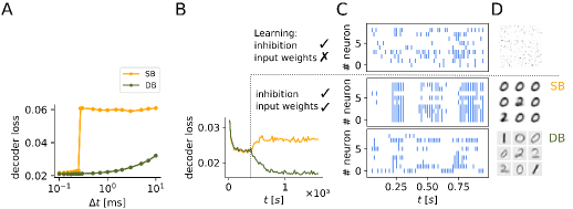
Fig 6: Dendritic balance prevents learning of redundant representations for long transmission delays. A Decoder loss of networks of 200 neurons coding for natural scenes for different transmission delays of inhibitory signals $\Delta t$. For transmission delays longer than $0.3\,\text{ms}$, Hebbian-like learning (SB) leads to highly inefficient representations and large decoder loss. In contrast, for networks learning with dendritic balance (DB), the decoder loss increases only moderately even for long transmission delays. The results are robust with respect to the stochasticity of firing $\Delta u$ and the firing rate $\rho$ (see supplementary Figure S8). B-D In another simulation experiment, networks of 9 neurons with long transmission delays of $3\,\text{ms}$ received images of MNIST digits 0,1 and 2 as inputs. B To demonstrate the impact of lateral inhibitory and input plasticity, first only inhibition was learned; later plasticity on input weights was turned on (dashed line). Inhibitory plasticity decorrelates responses and decreases the decoder loss. When input plasticity was turned on, Hebbian-like plasticity (SB) learned worse representations than random feed-forward weights, which is indicated by the increase in decoder loss. In contrast, our model with dendritic balance (DB) learned improved representations with substantially reduced decoder loss. C The poor performance of the classical model (SB) is a consequence of highly synchronous spiking responses to the inputs, whereas neurons fire asynchronously in the model with dendritic balance (DB). D Neurons in the classical model (SB) learn overly similar feed-forward weights, whereas neurons with dendritic balance learn feed-forward weights that capture the input space well.

In the presented model we assumed all-to-all inhibitory connectivity between coding neurons, which likely can be relaxed without losing the main benefits of the proposed learning scheme. All-to-all inhibitory connections are problematic, since connecting every neuron to all dendrites of other neurons in the population would even for moderately sized networks prove extremely costly. Moreover, in most neuron types the ratio of excitatory to inhibitory synapses is larger than one [30]. However, not all of the inhibitory connections in our model are relevant. First, only inhibitory connections matter that really contribute in achieving a tight balance at the dendrites, i.e. when the dendritic potential is correlated to the presynaptic inhibiting neuron (Eq 8). Second, the number of inhibitory connections could be further decreased by clustering correlated excitatory synapses, which is a well known phenomenon kastellakis_synaptic_2015chen_clustered_2012kleindienst_activity-dependent_2011. Clustered excitatory synapses could make use of the same inhibitory feedback if the inhibition provides a good estimate of the population code for all of these inputs. Third, inhibition is mediated by direct lateral connections between coding neurons, but less connections would be required if inhibition was mediated via interneurons. By incorporating inhibitory interneurons with broad feature selectivity, it would be possible to merge inhibitory connections that provide largely the same information. Finally, the number of inhibitory connections could be reduced by moving inhibition from the dendrites to the soma after learning. In our model, the second purpose of inhibition (besides informing excitatory plasticity) is to enable the concerted spiking of the neural population, which can also be guaranteed by somatic inhibition alone. Showing how exactly these reductions in wiring cost can be achieved, while maintaining the central benefits of the proposed learning scheme, should be a focus of future work.

A central element of our model is the dependence of synaptic plasticity on local membrane potentials, which has been argued to be a critical factor determining synaptic plasticity lisman_postsynaptic_2005lisman2010questionsartola1990differentngezahayo2000synaptic. Voltage-dependent plasticity is thought to be mediated mainly by the local Calcium concentration, which closely follows the local membrane potential tsien_calcium_1990kanemoto2011spatial and locally modulates neural plasticity [40]. Classical voltage-dependent plasticity rules assume that synaptic plasticity happens only in a highly depolarized regime, where deviations from a critical potential determine the sign of the induced plasticity clopath2010voltageshouval2002unified. Our derived rule can be reconciled with these classical rules if postsynaptic activity ($z_{j}$) brings the local potential into the highly depolarized regime, e.g. through back-propagating action potentials or dendritic plateau potentials [43], and then local input ($u^{i}_{j}$) determines the sign of plasticity. Furthermore, as required by our model, this voltage dependence implies that inhibition can have a major impact on excitatory synaptic plasticity locally bar-ilan_role_2013saudargiene_inhibitory_2015, which indeed has been found experimentally wang2014inhibitoryhennequin2017inhibitory. Therefore, while more work is necessary to understand what mechanisms might underlie its biophysical implementation, the proposed learning scheme is in principle compatible with voltage-dependent plasticity as mediated through local Calcium concentrations.

Our model thus provides an answer to the major open question what the functional implications of plasticity mechanisms based on local dendritic potentials could be hennequin2017inhibitorybono2017modelling. Other studies have explored this issue (for a review see [47]), for example with a focus on feature binding [48]. A theory related to ours suggests that voltage differences between soma and dendrite in two-compartment neurons present prediction errors brea2016prospectiveguerguiev2017towardssacramento2018dendritic. In contrast, our work shows that a coding error can be calculated from the mismatch between excitation and inhibition locally in individual dendritic compartments, such that the local membrane potential represents the coding error. We therefore propose that a central feature of synaptic plasticity based on local membrane potentials is to inform single synapse plasticity about plasticity-relevant activity of other neurons.

Ultimately, we can generate two directly measurable experimental predictions from our model: First, if input currents are locally unbalanced, inhibitory plasticity will learn to establish a local E-I balance. Second, our model predicts that the strength of local inhibition determines the sign of synaptic plasticity: During plasticity induction at excitatory feed-forward synapses, activating inhibitory neurons that target the same dendritic loci should lead to long-term depression of the excitatory synapses. We would expect this effect to persist, even if the inhibitory signal arrives shortly after the pre- and postsynaptic spiking.

To conclude, we here presented a learning scheme that facilitates highly cooperative population codes for complex stimuli in neural populations. Our results question pairwise Hebbian learning as a paradigm for representation learning, and suggest that there exists a direct connection between dendritic balance and synaptic plasticity.

Methods

Methods.sectionMethods.sectionMethodsMethodsMethods.section

Neural activity was simulated in discrete timesteps of length $\Delta t$. Images were presented as continuous inputs for 100ms, after 70ms they were linearly interpolated to the next image in order to avoid discontinuities in the input signal. For every experiment a learning and a test set was created. The networks learned online on the training set; in regular intervals the learning rules were turned off and the performance was evaluated on the test set. Performance was measured via the instantaneous decoder loss (Eq 1) by learning the decoder $D$ alongside the network. The respective update rule for the decoder is given by

$$\Delta D_{ij}\propto z_{j}(x_{i}-\textstyle{\sum_{k}}D_{ik}z_{k}).$$ (10)

For DB networks we propose two learning schemes with fast or slow inhibitory plasticity (detailed in SI). In order to reduce computation time for large networks, the analytical solution of optimal inhibitory weights $W^{i}_{jk}=-F_{ij}F_{ik}$ was used as an approximation of the proposed learning schemes. For Figure 3 the dendritic balance learning scheme with slow inhibitory plasticity is displayed. For the simulation of the correlated bars task (Fig 4) and natural scenes (Fig 5), as well as Figure 6 we used the analytical solution. When comparing the proposed learning schemes to the analytical solution on reference simulations (Fig S2, S3) they consistently found very similar network parameters and reached the same performance.

In early simulations we observed that coding performance is largely affected by the population rate, i.e. how many spikes can be used to encode the input signal. To avoid this effect when comparing the two learning schemes we additionally introduced a rapid compensatory mechanism to fix the firing rates which is realized by changing the thresholds $T_{j}$. We emphasize again that this adaptation is in principle not necessary to ensure stable network function. In fact, error-correcting balanced state inhibition can already be sufficient for a network to develop into a slow firing regime [12]. The fixed firing rate is enforced by adapting the threshold $T_{j}$ such that neurons are firing with a target firing rate $\rho$.

$$\Delta T_{j}\propto(s_{j}-\rho\>\Delta t)$$

Here, $\rho\>\Delta t$ is the mean number of spikes in a time window of size $\Delta t$ if a neuron would spike with rate $\rho$ and $s_{j}$ is a spike indicator which is $1$ if $z_{j}$ spiked in the last time $\Delta t$, otherwise $s_{j}=0$.

We furthermore aided the learning process by starting with a high stochasticity in spiking and slowly decreasing it towards the desired stochasticity. We observed that convergence of the networks to an efficient solution often was faster and more reliable with this method. Specifically for the simulations of correlated bars and natural scenes we started with a stochasticity of $\Delta u=1.0$. We then exponentially annealed it towards the final value $\Delta u^{*}$ by applying every timestep

$$\Delta u(t+1)=\Delta u(t)-\eta_{\Delta u}(\Delta u(t)-\Delta u^{*}).$$

Full derivations of the network dynamics and learning rules, supplementary figures containing additional information to simulation experiments, as well as simulation parameters, are provided in SI. Code for reproducing the main simulations is available online at https://github.com/Priesemann-Group/dendritic_balance.

Acknowledgements.sectionAcknowledgements.sectionAcknowledgementsAcknowledgementsAcknowledgements.section

Supplementary Information

SI.sectionSI.sectionSupplementary InformationSupplementary InformationSI.section

Symbols

• $\mathbf{X}_{0,T}=\{\mathbf{x}(t)|t\in\{0,...,T\}\}$: Input signal over time to be encoded

• $\mathbf{S}_{0,T}=\{\mathbf{s}(t)|t\in\{0,...,T\}\}$: Spikes of coding neurons

• $\mathbf{z}(t)$: ‘Outputs’ of coding neurons, proportional to evoked post-synaptic potentials

• $\mathbf{\hat{x}}(t)=D\mathbf{z}(t)$: Input signal reconstructed from network activity

• $D$: Decoder matrix of the decoder model

• $\sigma$: Variance of the decoder model

• $\mathbf{b}$: Spiking probability prior of decoder model

• $\theta$: Decoder model parameters $\{D,\sigma,\mathbf{b}\}$

• $F$: Excitatory feed forward weights

• $W$: Inhibitory recurrent weights connecting to the soma

• $W^{i}$: Inhibitory recurrent weights, connecting to the dendrites to input $i$.

• $T_{j}$: Soft threshold of neuron $j$

• $\Delta u$: Stochasticity of neural spiking

• $\tau$: Membrane time constant of leak

• $\eta_{(\cdot)}$: learning rate of parameter $(\cdot)$

• $\rho$: Target firing rate of neurons

• $1/Z(\cdot)$: Normalization of probability function

Stochastic neural dynamics

We simulated stochastic leaky integrate and fire neurons in discrete timesteps. The model can be seen as a special case of the spike response model with escape noise [52]. In timestep $t\in\{0,1,...,T\}$ with length $\Delta t$ neuron $j$ spikes with a probability

$$p_{\text{dyn}}\left(s_{j}(t)=1|\mathbf{x}(t),\mathbf{z}(t)\right)=p_{spike}(u_{j}(t))=\text{sig}\left(\frac{u_{j}(t)-T_{j}}{\Delta u}\right),$$ (11)

where $\text{sig}(x)=[1+\exp(-x)]^{-1}$, $u_{j}(t)$ is the membrane potential of the neuron, $T_{j}$ the firing threshold, $\Delta u$ defines how stochastic the spiking is and $s_{j}(t)$ is a spike indicator, which is $1$ if neuron $j$ spiked in time step $t$, otherwise $s_{j}=0$. Emitted spikes are then transmitted to other neurons and elicit post synaptic potentials (PSPs) $\mathbf{z}(t)$ with

$$z_{j}(t) =\sum_{t_{s}^{j}<t}\exp\left(-\frac{t-1-t_{s}^{j}}{\tau}\right),$$

which account for the leaky integration at the membrane. Here, $t_{s}^{j}$ are the spike times of neuron $j$ and $\tau$ the membrane time constant, which was chosen the same for all neurons. Please note that, in order to ease the upcoming derivations, we changed notation such that $t$ is the index of the discrete timestep and $\tau$ has the unit of timesteps. The time delay of PSP arrival of the length of one time step $\Delta t$ is interpreted as a finite traveling time of neural impulses over axons. The EPSPs together with input signal $\mathbf{x}(t)$ are then summed up linearly at the soma to give the membrane potential

$$u_{j}(t)=\sum_{i}F_{ji}x_{i}(t)+\sum_{k}W_{jk}z_{k}(t).$$

In order to model neurons that make use of dendritic balance we subdivided the somatic potentials such that they are sums of dendritic potentials: $u_{j}(t)=\sum_{i}u^{j}_{i}(t)$, where the dendritic potentials $u^{j}_{i}(t)=F_{ji}x_{i}(t)+\sum_{k}W^{i}_{jk}z_{k}(t)$. To summarize, stochastic neural dynamics are modeled through the spike probability $p_{\text{dyn}}\left(\mathbf{s}(t)|\mathbf{x}(t),\mathbf{z}(t)\right)$ with neural parameters $\{F,W,\mathbf{T},\Delta u\}$.

Learning an efficient code with expectation maximization

With the following derivations we provide a link between learned balanced state inhibition [12] and neural sampling in graphical models [13]. Furthermore we will address the linear case of the quite general problem which arises through explaining away effects, i.e. converging arrows in graphical models: Converging arrows imply that neurons should cooperate to encode the input and lead to non-localities in update rules when the neural dynamics are based on point neurons. In related studies this problem so far has been avoided in various ways, which all prevent the network from explaining the input through possibly correlated neurons simultaneously and thus limit coding versatility nessler_bayesian_2013bill_distributed_2015nessler2009stdpkappel_stdp_2014deneve_bayesian_2007.

The goal of neural spiking dynamics and plasticity throughout this paper is to find an efficient spike encoding, i.e. representing an input signal $\mathbf{X}_{0,T}=\{\mathbf{x}(t)|t\in\{0,...,T\}\}$ through a collection of spikes $\mathbf{S}_{0,T}=\{\mathbf{s}(t)|t\in\{0,...,T\}\}$. $\mathbf{X}_{0,T}$ can be seen here as an episode in an organisms life, which we will assume to be distributed according to $p^{*}(\mathbf{X}_{0,T})$. We say that $\mathbf{S}_{0,T}$ efficiently encodes $\mathbf{X}_{0,T}$ if the following two conditions are met:

1. $\mathbf{X}_{0,T}$ can be accurately estimated from $\mathbf{S}_{0,T}$ via a decoding model $p_{\theta}(\mathbf{X}_{0,T}|\mathbf{S}_{0,T})$.

2. The number of spikes emitted is small.

Hence we want to maximize the likelihood $p_{\theta}(\mathbf{X}_{0,T}|\mathbf{S}_{0,T})$ over both the decoding model parameters $\theta$ and the latent variables $\mathbf{S}_{0,T}$ sampled by the (constrained) network dynamics $p_{\text{dyn}}\left(\mathbf{s}(t)|\mathbf{x}(t),\mathbf{z}(t)\right)$.

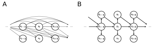
Fig S1: Graphical representation of the decoder model. A We consider a decoding model where readouts of inputs $\mathbf{x}(t)$ (denoted here as $\mathbf{x}_{t}$) are conditioned on preceding spikes $\mathbf{s}(t)$ (denoted as $\mathbf{s}_{t}$). B By introducing the spike traces $\mathbf{z}(t)$ into the model, the model factorizes over timesteps, which is equivalent to viewing it as a hidden Markov model (HMM) with hidden states $\{\mathbf{z}(t),\mathbf{s}(t)\}$.

To show how a stochastic spiking neural network can unsupervisedly learn such an encoding, we make use of the framework of online expectation-maximization (EM) learning [54]. EM-learning can find maximum-likelihood estimates for parameters of latent variable models (here $p_{\theta}(\mathbf{X}_{0,T},\mathbf{S}_{0,T})$) for observed data ($\mathbf{X}_{0,T}$). For these models it typically is intractable to marginalize out the latent variables ($\mathbf{S}_{0,T}$). In order to solve this problem one defines the log-likelihood lower bound

$$\begin{aligned} \mathcal{F}^{*}(\tilde{p},\theta)&=\left\langle\log p_{\theta}(\mathbf{X}_{0,T})-D_{KL}(\tilde{p}(\mathbf{S}_{0,T}|\mathbf{X}_{0,T})|p_{\theta}(\mathbf{S}_{0,T}|\mathbf{X}_{0,T}))\right\rangle_{p^{*}(\mathbf{X}_{0,T})}\\ &=\langle\log p_{\theta}(\mathbf{X}_{0,T},\mathbf{S}_{0,T})-\log\tilde{p}(\mathbf{S}_{0,T}|\mathbf{X}_{0,T})\rangle_{\tilde{p}(\mathbf{S}_{0,T}|\mathbf{X}_{0,T})p^{*}(\mathbf{X}_{0,T})}\end{aligned},$$ (12)

where $\tilde{p}(\mathbf{S}_{0,T}|\mathbf{X}_{0,T})$ can be any (tractable) probability distribution, which in our case will be given through $p_{dyn}$. Finding maximum-likelihood parameters $\theta$ can then be done by iteratively maximizing $\mathcal{F}^{*}(\tilde{p},\theta)$ with respect to $\tilde{p}$ (E-step) and $\theta$ (M-step). In the E-step $p_{\theta}$ is approximated by $\tilde{p}$ in order to estimate $\langle\log p_{\theta}(\mathbf{X}_{0,T},\mathbf{S}_{0,T})\rangle_{\tilde{p}(\mathbf{S}_{0,T}|\mathbf{X}_{0,T})p^{*}(\mathbf{X}_{0,T})}$ and in the M-step this approximation is used to improve the model. This algorithm is guaranteed to converge to a local minimum, also if $\mathcal{F}^{*}$ is maximized only partially in every iteration, which makes it applicable to online learning.

Appealing to this theory in the following we show that: (i) Given a linear decoding model, a stochastic spiking neural network can be connected such that it can sample an efficient encoding online. This relates model- and network-parameters. (ii) The decoding model can be optimized online in respect to the sampled dynamics of the network. (iii) Combining (i) (the E-step) and (ii) (the M-step) yields update rules that can be applied by a stochastic spiking neural network to optimize its parameters in order to encode its inputs.

Online encoding by spiking neural network

Let us consider the following decoding model and prior on the spiking probability (Fig S1)

$$p_{\theta}(\mathbf{X}_{0,T}|\mathbf{S}_{0,T})=\prod_{t}p_{\theta}(\mathbf{x}(t)|\mathbf{z}(t))=\prod_{t}\mathcal{N}_{\mathbf{x}(t)}(D\mathbf{z}(t),\Sigma)$$

$$p_{\theta}(\mathbf{S}_{0,T})=\prod_{t}p_{\theta}(\mathbf{s}(t)|\mathbf{z}(t))=\prod_{t}\frac{1}{Z(\mathbf{b})}\exp\left(\mathbf{s}(t)^{\top}\mathbf{b}\right)$$

with $\Sigma=\sigma^{2}I$ and parameters $\theta=\{D,\sigma,\mathbf{b}\}$. Notably this model asserts that at every time $t$, $\mathbf{x}(t)$ can be linearly decoded from spike traces $\mathbf{z}(t)$ with variance $\sigma^{2}$, where the spike traces are defined as before. Observe that the spike traces $\mathbf{z}(t)$ are deterministically defined given the preceding spikes $\mathbf{S}_{0,t-1}$. Since the model factorizes over time given the spike traces $\mathbf{z}(t)$, the log-likelihood lower bound (Eq 12) can be rewritten as

$$\mathcal{F}^{*}(p_{dyn},\theta)= \left\langle\sum_{t}\log p_{\theta}(\mathbf{x}(t),\mathbf{s}(t)|\mathbf{z}(t))-\log p_{dyn}(\mathbf{s}(t)|\mathbf{x}(t),\mathbf{z}(t))\right\rangle_{p_{dyn}(\mathbf{S}_{0,T}|\mathbf{X}_{0,T})p^{*}(\mathbf{X}_{0,T})}$$

$$= \left\langle\log p_{\theta}(\mathbf{X}_{0,T})\right\rangle_{p^{*}(\mathbf{X}_{0,T})}-$$

$$\left\langle\sum_{t}\log p_{dyn}(\mathbf{s}(t)|\mathbf{x}(t),\mathbf{z}(t))-\log p_{\theta}(\mathbf{s}(t)|\mathbf{X}_{t+1,T},\mathbf{z}(t))\right\rangle_{p_{dyn}(\mathbf{S}_{0,T}|\mathbf{X}_{0,T})p^{*}(\mathbf{X}_{0,T})}$$

Here we substituted $\tilde{p}(\mathbf{S}_{0,T}|\mathbf{X}_{0,T})=\prod_{t}p_{dyn}(\mathbf{s}(t)|\mathbf{x}(t),\mathbf{z}(t))$ and made use of the fact that spikes alter only the future decoding since they are independent of the past given $\mathbf{z}(t)$, i.e. $p_{\theta}(\mathbf{s}(t)|\mathbf{X}_{0,T},\mathbf{S}_{0,t-1})=p_{\theta}(\mathbf{s}(t)|\mathbf{X}_{t+1,T},\mathbf{z}(t))$.

We now perform the E-step. $\mathcal{F}^{*}$ is approximately maximized over $p_{\text{dyn}}$ if $p_{\text{dyn}}(\mathbf{s}(t)|\mathbf{x}(t),\mathbf{z}(t))\approx p_{\theta}(\mathbf{s}(t)|\mathbf{X}_{t+1,T},\mathbf{z}(t))$ at every time $t$. However, this poses two problems: (i) $p_{\text{dyn}}$ depends only on $\mathbf{x}(t)$ while the spike probability in the model is based on future values $\mathbf{X}_{t+1,T}$, which are not available to the network. (ii) In order to compute $p_{\theta}(\mathbf{s}(t)|\mathbf{X}_{t+1,T},\mathbf{z}(t))=\sum_{\mathbf{S}_{t+1,T}}p_{\theta}(\mathbf{S}_{t,T}|\mathbf{X}_{t+1,T},\mathbf{z}(t))$ future spikes have to be marginalized out, which is intractable. For the purpose of this paper we introduced simple approximations that solve these problems and work well in practice for our inputs. Specifically we assumed input- and network activity to be approximately constant over time. Hence all future inputs $\mathbf{x}(t^{\prime})\in\mathbf{X}_{t+1,T}$ were assumed to be known to be $\mathbf{x}(t^{\prime})=\mathbf{x}(t)$. Future network activity (independent of the current spike $\mathbf{s}(t)$) was assumed to be well approximated by a single trajectory, where neural outputs $\mathbf{z}(t)$ were constant. With this we can compute

$$\sum_{\mathbf{S}_{t+1,T}} p_{\theta}(\mathbf{s}(t)|\mathbf{X}_{t+1,T},\mathbf{z}(t),\mathbf{S}_{t+1,T})p_{\theta}(\mathbf{S}_{t+1,T}|\mathbf{X}_{t+1,T},\mathbf{z}(t))$$

$$\approx \prod_{t^{\prime}=t}^{T}p_{\theta}\left(\mathbf{s}(t)|\mathbf{x}(t^{\prime})=\mathbf{x}(t),\mathbf{z}(t^{\prime})=\mathbf{z}(t)+\mathbf{s}(t)\exp\left(-\frac{t^{\prime}-1-t}{\tau}\right)\right)$$

$$= \frac{1}{Z(\theta,\mathbf{x})}\exp\left(\mathbf{s}(t)^{\top}\mathbf{b}\right)\prod_{t^{\prime}=t+1}^{T}\exp\left(\frac{\mathbf{z}(t^{\prime})^{\top}}{\sigma^{2}}[D^{\top}\mathbf{x}(t^{\prime})-\frac{1}{2}D^{\top}D\mathbf{z}(t^{\prime})]\right)$$

$$= \frac{1}{Z(\theta,\mathbf{x})}\exp\left(\mathbf{s}(t)^{\top}\mathbf{b}\right)\prod_{t^{\prime}=t+1}^{T}\exp\Bigg{(}\frac{\left(\mathbf{z}(t)+\mathbf{s}(t)\exp\left(-\frac{t^{\prime}-1-t}{\tau}\right)\right)^{\top}}{\sigma^{2}}\Bigg{[}D^{\top}\mathbf{x}(t)-$$

$$-\frac{1}{2}D^{\top}D\left(\mathbf{z}(t)+\mathbf{s}(t)\exp\left(-\frac{t^{\prime}-1-t}{\tau}\right)\right)\Bigg{]}\Bigg{)}$$

$$= \frac{1}{Z(\theta,\mathbf{x},\mathbf{z})}\exp\left(\mathbf{s}(t)^{\top}\left[\mathbf{b}+\frac{\tau}{\sigma^{2}}D^{\top}\mathbf{x}(t)-\frac{\tau}{\sigma^{2}}D^{\top}D\left(\mathbf{z}(t)+\frac{1}{4}\mathbf{s}(t)\right)\right]\right)$$

$$= \frac{1}{Z(\theta,\mathbf{x},\mathbf{z})}\exp\left(\mathbf{s}(t)^{\top}\left[\mathbf{b}+\frac{\tau}{\sigma^{2}}D^{\top}\mathbf{x}(t)-\frac{\tau}{\sigma^{2}}D^{\top}D\mathbf{z}(t)-\frac{1}{4}\frac{\tau}{\sigma^{2}}\text{diag}(D^{\top}D)\right]\right)$$

where we approximated $\sum^{T}_{t^{\prime}=t+1}\exp(-\frac{t^{\prime}-1-t}{\tau})\approx\tau$ (that is $\tau$ and $T$ large) and the last equality follows if timesteps are sufficiently small such that only one neuron spikes per timestep. Comparing with the network dynamics (Eq 11) from this we can conclude that a network that performs approximate online sampling from $p_{\theta}(\mathbf{S}_{0,T}|\mathbf{X}_{0,T})$ has parameters

$$F =D^{\top}$$ (13)

$$W =-D^{\top}D$$

$$T_{j} =\frac{1}{4}W_{jj}-\frac{\sigma^{2}}{\tau}b_{j}$$

$$\Delta u =\frac{\sigma^{2}}{\tau}$$

These results are similar to those yielded by a greedy spike encoding scheme [12]. Please note that the sampling could be improved by using advanced sampling schemes, such as rejection sampling [16].

Online-learning of an optimal decoder

As we have shown, the network dynamics implement an approximation of the E-step if the network parameters are chosen correctly. We will now use these samples produced by the network to incrementally improve the parameters of the decoding model in the M-step.

Recall that in the M-step we want to maximize under $\theta$

$$\left\langle\sum_{t}\log p_{\theta}(\mathbf{x}(t),\mathbf{s}(t)|\mathbf{z}(t))\right\rangle_{p_{dyn}(\mathbf{S}_{0,T}|\mathbf{X}_{0,T})p^{*}(\mathbf{X}_{0,T})}.$$

Updates of the decoder model parameters should thus follow the gradient

$$\Delta\theta=\tilde{\eta}_{\theta}\frac{\partial\mathcal{F}^{*}}{\partial\theta}=\tilde{\eta}_{\theta}\left\langle\sum_{t}\frac{\partial}{\partial\theta}\log p_{\theta}(\mathbf{x}(t),\mathbf{s}(t)|\mathbf{z}(t))\right\rangle_{p_{dyn}(\mathbf{S}_{0,T}|\mathbf{X}_{0,T})p^{*}(\mathbf{X}_{0,T})}$$

In this paper we’re only interested in the decoder weights $D_{ij}$ from neuron $j$ to input $i$, where the derivation yields

$$\Delta D_{ij}=\tilde{\eta}_{D}\left\langle\sum_{t}\sigma^{-2}z_{j}(t)\left(x_{i}(t)-\sum_{k}D_{ik}z_{k}(t)\right)\right\rangle_{p_{dyn}(\mathbf{S}_{0,T}|\mathbf{X}_{0,T})p^{*}(\mathbf{X}_{0,T})}$$

Here, $\tilde{\eta}_{D}$ is the update step size and $\sigma^{2}$ the variance of the decoder model. Note that in the following we will drop the dependence of the learning rate on $\sigma^{2}$, which has its motivation in covariant optimization [55]. In covariant optimization, the gradient is multiplied by the inverse curvature of the loss function, because step size should be decreased when the curvature of the loss function is high. Since the curvature of the likelihood is proportional to the inverse variance, the variance drops out to yield a covariant gradient. This yields the update rule

$$\Delta D_{ij}=\tilde{\eta}_{D}\left\langle\sum_{t}z_{j}(t)\left(x_{i}(t)-\sum_{k}D_{ik}z_{k}(t)\right)\right\rangle_{p_{dyn}(\mathbf{S}_{0,T}|\mathbf{X}_{0,T})p^{*}(\mathbf{X}_{0,T})}$$

Online approximation If many episodes $\mathbf{X}_{0,T}$ as sampled from $p^{*}(\mathbf{X}_{0,T})$ are presented in succession and spikes are sampled as outlined above, the average over samples from $p_{dyn}$ can be replaced by an average over time

$$\left\langle\sum_{t}\cdot\right\rangle_{p_{dyn}(\mathbf{S}_{0,T}|\mathbf{X}_{0,T})p^{*}(\mathbf{X}_{0,T})}\approx\sum_{t}\left\langle\cdot\right\rangle_{t}.$$

If the update rules are performed every timestep this lets us rewrite them as

$$\delta D_{ij}=\eta_{D}z_{j}(t)\left(x_{i}(t)-\sum_{k}D_{ik}z_{k}(t)\right)$$ (14)

This requires, however, that the learning rate $\eta_{D}$ is sufficiently small such that changes in $D_{ij}$ are negligible in a sufficiently long time window $T^{\prime}$. In that case, summing the equation over time window $T^{\prime}$ yields

$$\sum_{t=0}^{T^{\prime}}\delta{D_{ij}} =\eta_{D}T^{\prime}\left\langle z_{j}(t)\left(x_{i}(t)-\sum_{k}D_{ik}z_{k}(t)\right)\right\rangle_{t=0}^{T^{\prime}}$$

$$\overset{T^{\prime}\rightarrow T}{\approx}\Delta D_{ij},$$

where the learning rates are related via $\tilde{\eta}_{D}=\eta_{D}T^{\prime}$. A more refined statement can be made by rewriting the update equation as

$$\Delta D_{ij}=\tilde{\eta}_{D}\left(\left\langle z_{j}(t)x_{i}(t)\right\rangle_{p_{dyn}(\mathbf{S}_{0,T}|\mathbf{X}_{0,T})p^{*}(\mathbf{X}_{0,T})}-\sum_{k}D_{ik}\left\langle z_{j}(t)z_{k}(t)\right\rangle_{p_{dyn}(\mathbf{S}_{0,T}|\mathbf{X}_{0,T})p^{*}(\mathbf{X}_{0,T})}\right)$$

This makes explicit that the only information required to compute the gradient of the decoder weights are the correlations between neural outputs and inputs and in between neural outputs over the input sequences. Thus in practice, the learning rate $\eta_{D}$ is ideally chosen as large as possible to allow fast learning, but also sufficiently small such that weight updates are performed with respect to a time window that provides a good estimate of correlations under the whole sampled spike trains.

Online-learning of network parameters

So far we showed that the parameters of a network that samples from a decoder model are directly connected to the parameters of the model. We also showed how the decoder weights have to be updated such that they maximize the model likelihood over the generated samples. We will now combine these two results to find update rules for neural parameters directly, that can be used by neurons to learn an efficient encoding without supervision online. To this end we will first show how an approximation to the previously derived gradients can be implemented by regular stochastic LIF neurons. In a second step we will show how a better approximation can be realized by neurons with dendritic compartments. The central insight for all derivations will be that learning an E-I balance on membrane potentials corresponds to the learning of a decoder to the excitatory inputs times a transformation matrix that brings them into the space of the membrane potentials.

Somatic balance approximation

Feed-forward weights
From the equality $F=D^{\top}$ (Eq 13) derived earlier and the update rule for $D$ (Eq 14) we directly arive at

$$\delta F_{ji}=\eta_{F}z_{j}(t)\left(x_{i}(t)-\sum_{k}F_{ki}z_{k}(t)\right)$$

We follow previous approaches [12] and ommit contributions to the decoding $\sum_{k}F_{ki}z_{k}(t)$ that are not available for the neuron, which is equivalent to assuming that neural spiking in the population is uncorrelated $\forall j\neq k:\langle z_{j}(t)z_{k}(t)\rangle_{t}\approx 0$. This yields the regularized Hebbian rule

$$\delta F_{ji}=\eta_{F}z_{j}(t)\left(x_{i}(t)-F_{ji}z_{j}(t)\right)$$ (15)

Inhibitory weights
This rule will follow the optimal decoder gradient if spikes are indeed uncorrelated. However, if this is not the case the solution will be suboptimal and furthermore the previously derived inhibition $W=-D^{\top}D$ together with the suboptimal weights $F$ does not enable a reasonable encoding anymore. Both problems can be addressed by observing that for the optimal membrane potential we derived

$$\mathbf{u}^{opt}(t)=D^{\top}\mathbf{x}(t)-D^{\top}D\mathbf{z}(t)=D^{\top}(\mathbf{x}(t)-D\mathbf{z}(t))$$

i.e. the potentials are proportional to the decoding error. This can be approximately guaranteed even if the feed-forward weights are suboptimal (but not zero) by setting $W=-FD$, since then

$$\mathbf{u}(t)=F\mathbf{x}(t)-FD\mathbf{z}(t)=F(\mathbf{x}(t)-D\mathbf{z}(t))\overset{\approx}{\propto}\mathbf{u}^{opt}(t)$$

To make sure that neurons adapt their encoding for an optimal decoder, inhibitory weights will adapt along the gradient of decoder weights. For fixed encoder weights $F$ this yields

$$\delta{W}_{jk} =-\sum_{i}F_{ji}\delta{D}_{ik}$$ (16)

$$=-\eta_{W}z_{k}(t)\left(\sum_{i}F_{ji}x_{i}(t)-\sum_{i,l}F_{ji}D_{il}z_{l}(t)\right)$$

$$=-\eta_{W}z_{k}(t)\left(\sum_{i}F_{ji}x_{i}(t)+\sum_{l}W_{jl}z_{l}(t)\right)$$

$$=-\eta_{W}z_{k}(t)u_{j}(t)$$

This shows that through an E-I balance, this rule for $W$ self-consistently finds the correct decoder ‘inside’ of the inhibitory weights, and hence allows the projection of the right decoding error $x-Dz$ through lateral inhibition. Thereby the inhibition ensures a reasonable encoding even if feed-forward weights are not learned optimally. Since in the equation above $F_{ji}$ is assumed constant, we chose the learning rate $\eta_{W}$ 2-4 times larger than $\eta_{F}$. In simulations we found that inhibitory weights that evolve under Eq 16 indeed converged to $W=-FD$, where $D$ is the optimal decoder weights obtained under the non-local update rule Eq 14 .

Learning encoder weights with dendritic balance In the following we devise examples for local plasticity rules for feed-forward inputs that follow the correct gradient of the likelihood lower bound. Locality requires that the decoding of other neurons is made available at the synapse, which can then be used to find the correct gradient. We argue that this can be mediated by dendritic inhibitory connections $W^{i}$ that target dendrites where the feed-forward input $i$ has formed a synapse. Due to the locality in space, the membrane potential $u^{i}_{j}$ in the vicinity of synapse $i$ on that dendrite only integrates inputs that are present locally, i.e.

$$u^{i}_{j}(t)=\underbrace{F_{ji}x_{i}(t)}_{\text{excitatory input}}+\underbrace{\textstyle{\sum_{k}}W^{i}_{jk}z_{k}(t)}_{\text{dendritic inhibition}}.$$ (17)

We then assume a regime where currents from the dendrites are summed linearly, such that the total membrane potential at the soma is given by $u_{j}(t)=\sum_{i}u_{j}^{i}(t)$. Similar to somatic inhibition, we will show that dendritic inhibitory connections can locally learn an optimal decoding of neural PSPs $\mathbf{z}$ by enforcing dendritic balance of excitatory and inhibitory inputs. The central feature of this approach is that inhibition and excitation both use the dendritic potential for learning, which requires their cooperation. We here show two possible mechanisms that realize this and yield very similar behaviour to the analytical solution (Fig S2, S3).

Slow feed-forward adaptation
One possibility to ensure the cooperation of feed-forward and inhibitory weights is to separate the timescales on which they are adapting. To that end we make the optimal inhibition ansatz similar to before $W_{jk}^{i}=-F_{ji}D_{ik}$. Then, changing inhibitory weights in the direction of the decoder gradient of Eq 14 yields

$$\delta{W}_{jk}^{i}= -F_{ji}\delta{D}_{ik}$$

$$= -\eta_{W}z_{k}(t)(F_{ji}x_{i}(t)-\textstyle{\sum_{l}}F_{ji}D_{il}z_{l}(t))$$

$$= -\eta_{W}z_{k}(t)(F_{ji}x_{i}(t)+\textstyle{\sum_{l}}W_{jl}^{i}z_{l}(t))$$

$$= -\eta_{W}z_{k}(t)u_{j}^{i}(t).$$

where we again assumed that changes in feed-forward weights are slow and can be neglected, and $\eta_{W}=\eta_{D}$. We conclude that enforcing dendritic balance by inhibitory plasticity is equivalent to locally optimizing a decoder $D_{ik}=-W_{jk}^{i}/F_{ji}$.

The correct gradient of the decoder weights can also be calculated locally, but it can’t be applied to the feed-forward weights directly since this would contradict the previously made assumption of slow changes in feed-forward weights. However, it is possible to locally integrate the correct gradient and use this to adapt feed-forward weights slowly, with a delay. To this end we introduce the local integration variable $I_{ji}=F_{ji}D_{ij}$, which adapts according to the decoder gradient times $F_{ji}$

$$\delta{I}_{ji}= \eta_{I}F_{ji}z_{j}(t)\left(x_{i}(t)-\textstyle{\sum_{k}}D_{jk}z_{k}(t)\right)$$

$$= \eta_{I}z_{j}(t)u^{i}_{j}(t)$$

with $\eta_{I}=\eta_{D}$. $F_{ji}$ then can slowly follow $D_{ij}$ via

$$\delta{F}_{ji}= \eta_{F}(I_{ji}/F_{ji}-F_{ji})$$

with $\eta_{F}\ll\eta_{D}$. Note that for $F_{ji}=0$ the gradient for $F_{ji}$ is not defined. In this case the learning process could be kickstarted via simple Hebbian learning on $F_{ji}$. It is also possible to assume very small but nonzero weights from the start. Note also that the equation $W_{jk}^{i}=-F_{ji}D_{ik}$ has to hold at the start of learning, which can be guaranteed by simply choosing $W_{jk}^{i}=F_{ji}=0$. To summarize, slow feed-forward adaptation leads to neural parameters $W^{i}_{jk}=-F_{ji}D_{ik}$ and $F_{ji}=D_{ij}$. This shows that input synapses slowly can evolve to minimize the decoder error along its gradient using only local information.

Simultaneous adaptation of feed-forward and inhibitory weights
In principle it would also be possible to adapt feed-forward and inhibitory weights simultaneously without a separation of timescales. However, calculating the gradient for the derived inhibitory weights is locally not feasible, since we find

$$\delta{W}_{jk}^{i}= -D_{ji}\delta{D}_{ik}-\delta D_{ji}{D}_{ik}$$

$$= -\eta_{D}(z_{k}(t)u_{j}^{i}(t)+z_{j}(t)u_{k}^{i}(t)).$$

Empirically we found that the contralateral contributions $z_{j}(t)u_{k}^{i}(t)$ to the gradient can be approximated by the accessible contributions $z_{k}(t)u_{j}^{i}(t)$. We thus approximate $\langle z_{j}(t)u_{k}^{i}(t)\rangle_{t}\approx\langle z_{k}(t)u_{j}^{i}(t)\rangle_{t}$. While this equation does not hold for all $i,j,k$, we still find that the resulting learned contributions to the dendritic potentials have the correct magnitude, hence enabling feed-forward learning. The gradient for the inhibitory weights now are

$$\delta{W}_{jk}^{i}= -\eta_{W}z_{k}(t)u_{j}^{i}(t),$$

where $\eta_{W}=2\eta_{D}$.

Assuming the correct inhibition ${W}_{jk}^{i}=-D_{ji}D_{ki}$ we can find the decoded population encoding locally at the dendrite. From the self-consistency $F_{ji}=D_{ij}$ and Eq 17 we have the relation

$$\sum_{k}D_{jk}z_{k}(t)=\frac{F_{ji}x_{i}(t)-u^{i}_{j}(t)}{F_{ji}}$$

With this we can implement the learning of feed-forward weights in way that highlights its similarity to previous approaches (Eq 15)

$$\delta F_{ji}=\eta_{F}z_{j}(t)\left(x_{i}(t)-\frac{F_{ji}x_{i}(t)-u^{i}_{j}(t)}{F_{ji}}\right),$$

i.e. the rule is a regularized Hebbian plasticity rule. Again, for very small $F_{ji}$ the regularization becomes unstable, but can be left away (since it should go to zero) leaving a purely Hebbian rule. For the derivation we used $\eta_{F}=\eta_{D}$, which implies that we should choose $\eta_{W}\approx 2\eta_{F}$. A relatively slow inhibitory learning that coincides with feed-forward plasticity has also been reported by [56].

In simulations we verified that the approximations we made for this learning scheme are adequate and yield feed forward weights for which $F_{ji}=D_{ij}$ holds with high accuracy. Note that the network found by the presented learning scheme only corresponds to the decoding model if $\eta_{W}\approx 2\eta_{F}$. However, if the inhibitory learning is faster this only results in a rescaling of feed-forward weights by a factor of $2\eta_{F}/\eta_{W}$, since their adaptation is too slow by this factor. This means that in this case the “correct” dynamics of the network can be recovered via a rescaling of all weights, or equivalently, with firing rate adaptation a change in the stochasticity of spiking $\Delta u$ by a factor of $2\eta_{F}/\eta_{W}$.

Rapid firing rate adaptation In the Bayesian framework Habenschuss and colleagues have shown that a rapid rate adaptation can be interpreted as a constraint on the variational approximation in the E-step [57]. For the resulting constrained optimization formally a Lagrange multiplier is introduced which ‘overwrites’ the analytic threshold $T_{j}=\frac{1}{4}W_{jj}-\sigma^{2}\tau^{-1}b_{j}$. We will not make a notational difference between the two thresholds here. The fixed firing rate is enforced by adapting the threshold $T_{j}$ such that neurons are firing with a target firing rate $\rho$.

$$\delta T_{j}=\eta_{T}(s_{j}-\rho\>\Delta t)$$

Here, $\rho\>\Delta t$ is the mean number of spikes in a time window of size $\Delta t$ if a neuron would spike with rate $\rho$ and $s_{j}$ is a spike indicator which is $1$ if $z_{j}$ spiked in the last time $\Delta t$, otherwise $s_{j}=0$. Since this is a constraint that is applied in the E-step, the learning rate $\eta_{T}$ should be large.

Datasets

MNIST

The standard MNIST database of handwritten digits was used [58]. Images were scaled down from $28\times 28$ to $16\times 16$ pixels. No further preprocessing was applied.

Correlated bars

See description in Figure 4A. Pixels where bars are displayed (also in the case of overlap) were set to the value 1.0, pixels without bars were set to 0.0.

Natural scenes

Images for natural scenes were taken from [59]. A simple preprocessing was applied to ensure that they can be modeled by spiking neurons. Importantly we required that input is always positive. Every image $\mathbf{\chi}$ in the database was whitened, which can be seen as an approximation of retinal on/off-cell preprocessing, where one on-cell and one off-cell with overlapping fields are lumped together in a single value $\chi_{i}$ which can be positive or negative. We separated every value $\chi_{i}$ into two values $x^{\prime}_{2i}=\chi_{i}$ and $x^{\prime}_{2i+1}=-\chi_{i}$. We then applied a continuous nonlinear activation function to ensure that activations are positive and bimodally distributed (i.e. mostly close to either 0.0 or 1.0): $x_{i}=\text{sig}(3.2(x^{\prime}_{i}-0.8))$, where $\text{sig}(x)=1/(1+\exp{(-x)})$. For the display of learned weights we merge corresponding values again and display $x_{2i}-x_{2i+1}$.

Parameters

For all tasks parameters were tuned to ensure that networks operate well. DB denotes networks where the analytic solution given the decoder was used for network dynamics. DB delayed are networks with slow feed-forward adaptation, DB simultaneous are networks with parallel adaptation of feed-forward and inhibitory weights. SB are networks learning with somatic balance. When the parameter $\eta_{\Delta u}$ is present the stochasticity of spiking was annealed starting from 1.0 with rate $\eta_{\Delta u}$.

MNIST (Fig 3, 6, S2)

Parameter	DB	DB simultaneous	DB delayed	SB
$\Delta t$	0.1ms	0.1ms	0.1ms	0.1ms
$\tau$	10ms	10ms	10ms	10ms
$\Delta u$	0.1	0.1	0.1	0.1
$\rho$	20$\text{s}^{-1}$	20$\text{s}^{-1}$	20$\text{s}^{-1}$	20$\text{s}^{-1}$
$\eta_{T}$	$5.0\cdot 10^{-3}$	$3.0\cdot 10^{-3}$	$5.0\cdot 10^{-4}$	$5.0\cdot 10^{-3}$
$\eta_{F}$	-	$3.0\cdot 10^{-6}$	$4.0\cdot 10^{-7}$	$5.0\cdot 10^{-6}$
$\eta_{I}$	-	-	$4.0\cdot 10^{-5}$	-
$\eta_{W}$	-	$6.0\cdot 10^{-6}$	$4.0\cdot 10^{-5}$	$1.0\cdot 10^{-5}$
$\eta_{D}$	$5.0\cdot 10^{-6}$	$3.0\cdot 10^{-6}$	$5.0\cdot 10^{-6}$	$5.0\cdot 10^{-6}$

Correlated bars (Fig 4, S3)

Parameter	DB	DB simultaneous	DB delayed	SB
$\Delta t$	1.0ms	1.0ms	1.0ms	1.0ms
$\tau$	10ms	10ms	10ms	10ms
$\Delta u^{*}$	0.1	0.1	0.1	0.1
$\eta_{\Delta u}$	$7.0\cdot 10^{-8}$	$7.0\cdot 10^{-8}$	$7.0\cdot 10^{-8}$	$7.0\cdot 10^{-8}$
$\rho$	15$\text{s}^{-1}$	15$\text{s}^{-1}$	15$\text{s}^{-1}$	15$\text{s}^{-1}$
$\eta_{T}$	$1.0\cdot 10^{-2}$	$1.0\cdot 10^{-2}$	$5.0\cdot 10^{-2}$	$1.0\cdot 10^{-2}$
$\eta_{F}$	-	$5.0\cdot 10^{-5}$	$1.0\cdot 10^{-7}$	$5.0\cdot 10^{-5}$
$\eta_{I}$	-	-	$5.0\cdot 10^{-5}$	-
$\eta_{W}$	-	$1.0\cdot 10^{-4}$	$5.0\cdot 10^{-5}$	$1.0\cdot 10^{-4}$
$\eta_{D}$	$5.0\cdot 10^{-5}$	$5.0\cdot 10^{-5}$	$5.0\cdot 10^{-5}$	$5.0\cdot 10^{-5}$

Natural scenes (Fig 5, 6, S4, S5, S6, S7, S8)

Parameter	DB	SB
$\Delta t$	0.2ms	0.2ms
$\tau$	10ms	10ms
$\Delta u^{*}$	0.13	0.13
$\eta_{\Delta u}$	$7.0\cdot 10^{-8}$	$7.0\cdot 10^{-8}$
$\rho\cdot\text{\# neurons}$	1000$\text{s}^{-1}$	1000$\text{s}^{-1}$
$\eta_{T}$ until $t=6000$s	$6.0\cdot 10^{-3}$	$6.0\cdot 10^{-3}$
$\eta_{T}$ until $t=\infty$	$4.0\cdot 10^{-3}$	$4.0\cdot 10^{-3}$
$\eta_{F}$ until $t=6000$s	-	$4.0\cdot 10^{-5}$
$\eta_{F}$ until $t=\infty$	-	$3.0\cdot 10^{-5}$
$\eta_{W}$ until $t=6000$s	-	$10.0\cdot 10^{-5}$
$\eta_{W}$ until $t=\infty$	-	$7.0\cdot 10^{-5}$
$\eta_{D}$ until $t=6000$s	$4.0\cdot 10^{-5}$	$4.0\cdot 10^{-5}$
$\eta_{D}$ until $t=\infty$	$3.0\cdot 10^{-5}$	$3.0\cdot 10^{-5}$

Supplementary figures

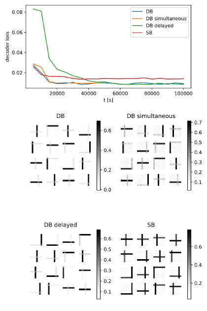
Fig S3: Comparison of the different learning schemes on the bars task with $p=0.8$.

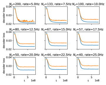
Fig S4: All learning curves for the natural scenes task (Fig 5).

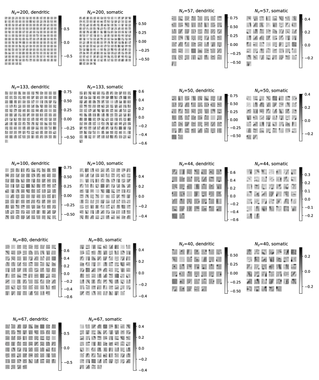
Fig S5: All learned weights for the natural scenes task (Fig 5).

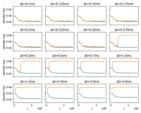
Fig S6: All learning curves for the natural scenes task for different timesteps (Fig 6A).

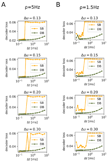
Fig S8: The results in Figure 6A are robust in respect to the stochasticity of firing $\Delta u$ and firing rate $\rho$. We tested firing rates of A $\rho=5\text{Hz}$, where learning is mostly stable, and B $\rho=1.5\text{Hz}$, where learning becomes slightly unstable. For higher stochasticity (larger $\Delta u$) neural firing becomes extremely random, for more deterministic neurons (smaller $\Delta u$) learning often does not converge.

References

- 1. H.. Barlow “Possible Principles Underlying the Transformations of Sensory Messages” In Sensory Communication The MIT Press, 2012, pp. 216–234 DOI: 10.7551/mitpress/9780262518420.003.0013
- 2. Biswa Sengupta, Simon B. Laughlin and Jeremy E. Niven “Balanced Excitatory and Inhibitory Synaptic Currents Promote Efficient Coding and Metabolic Efficiency” In PLOS Computational Biology 9.10, 2013, pp. e1003263 DOI: 10.1371/journal.pcbi.1003263
- 3. Joseph J Atick and A Norman Redlich “Towards a theory of early visual processing” In Neural Computation 2.3 MIT Press, 1990, pp. 308–320
- 4. Bruno A. Olshausen and David J. Field “Emergence of simple-cell receptive field properties by learning a sparse code for natural images” In Nature 381.6583, 1996, pp. 607–609 DOI: 10.1038/381607a0
- 5. C van Vreeswijk and Haim Sompolinsky “Chaotic balanced state in a model of cortical circuits” In Neural computation 10.6 MIT Press, 1998, pp. 1321–1371
- 6. Sophie Denève and Christian K. Machens “Efficient codes and balanced networks” In Nature Neuroscience 19.3, 2016, pp. 375–382 DOI: 10.1038/nn.4243
- 7. T.. Vogels et al. “Inhibitory Plasticity Balances Excitation and Inhibition in Sensory Pathways and Memory Networks” In Science 334.6062, 2011, pp. 1569–1573 DOI: 10.1126/science.1211095
- 8. Nima Dehghani et al. “Dynamic Balance of Excitation and Inhibition in Human and Monkey Neocortex” In Scientific Reports 6.1, 2016, pp. 1–12 DOI: 10.1038/srep23176
- 9. Bilal Haider, Alvaro Duque, Andrea R. Hasenstaub and David A. McCormick “Neocortical Network Activity In Vivo Is Generated through a Dynamic Balance of Excitation and Inhibition” In Journal of Neuroscience 26.17, 2006, pp. 4535–4545 DOI: 10.1523/JNEUROSCI.5297-05.2006
- 10. Peter Földiak “Forming sparse representations by local anti-Hebbian learning” In Biological cybernetics 64.2 Springer, 1990, pp. 165–170
- 11. Ralph Linsker “Local synaptic learning rules suffice to maximize mutual information in a linear network” In Neural Computation 4.5 MIT Press, 1992, pp. 691–702
- 12. Wieland Brendel et al. “Learning to represent signals spike by spike” In PLoS computational biology 16.3 Public Library of Science San Francisco, CA USA, 2020, pp. e1007692
- 13. Bernhard Nessler, Michael Pfeiffer, Lars Buesing and Wolfgang Maass “Bayesian Computation Emerges in Generic Cortical Microcircuits through Spike-Timing-Dependent Plasticity” In PLoS Computational Biology 9.4, 2013, pp. e1003037 DOI: 10.1371/journal.pcbi.1003037
- 14. Johannes Bill et al. “Distributed Bayesian Computation and Self-Organized Learning in Sheets of Spiking Neurons with Local Lateral Inhibition” In PLOS ONE 10.8, 2015, pp. e0134356 DOI: 10.1371/journal.pone.0134356
- 15. Bernhard Nessler, Michael Pfeiffer and Wolfgang Maass “STDP enables spiking neurons to detect hidden causes of their inputs” In Advances in neural information processing systems, 2009, pp. 1357–1365
- 16. David Kappel, Bernhard Nessler and Wolfgang Maass “STDP Installs in Winner-Take-All Circuits an Online Approximation to Hidden Markov Model Learning” In PLoS Computational Biology 10.3, 2014, pp. e1003511 DOI: 10.1371/journal.pcbi.1003511
- 17. Martin Boerlin, Christian K Machens and Sophie Denève “Predictive coding of dynamical variables in balanced spiking networks” In PLoS computational biology 9.11 Public Library of Science, 2013
- 18. Camille E. Rullán Buxó and Jonathan W. Pillow “Poisson balanced spiking networks”, 2019 DOI: 10.1101/836601
- 19. David J Tolhurst, J Anthony Movshon and Andrew F Dean “The statistical reliability of signals in single neurons in cat and monkey visual cortex” In Vision research 23.8 Elsevier, 1983, pp. 775–785
- 20. Adrien Wohrer, Mark D Humphries and Christian K Machens “Population-wide distributions of neural activity during perceptual decision-making” In Progress in neurobiology 103 Elsevier, 2013, pp. 156–193
- 21. James FA Poulet and Carl CH Petersen “Internal brain state regulates membrane potential synchrony in barrel cortex of behaving mice” In Nature 454.7206 Nature Publishing Group, 2008, pp. 881–885
- 22. Jianing Yu and David Ferster “Membrane potential synchrony in primary visual cortex during sensory stimulation” In Neuron 68.6 Elsevier, 2010, pp. 1187–1201
- 23. Rajesh PN Rao and Dana H Ballard “Predictive coding in the visual cortex: a functional interpretation of some extra-classical receptive-field effects” In Nature neuroscience 2.1 Nature Publishing Group, 1999, pp. 79–87
- 24. Rafal Bogacz “A tutorial on the free-energy framework for modelling perception and learning” In Journal of mathematical psychology 76 Elsevier, 2017, pp. 198–211
- 25. Karl Friston “A theory of cortical responses” In Philosophical transactions of the Royal Society B: Biological sciences 360.1456 The Royal Society London, 2005, pp. 815–836
- 26. Guosong Liu “Local structural balance and functional interaction of excitatory and inhibitory synapses in hippocampal dendrites” In Nature Neuroscience 7.4, 2004, pp. 373–379 DOI: 10.1038/nn1206
- 27. Daniel Maxim Iascone et al. “Whole-neuron synaptic mapping reveals spatially precise excitatory/inhibitory balance limiting dendritic and somatic spiking” In Neuron Elsevier, 2020
- 28. Jennifer N. Bourne and Kristen M. Harris “Coordination of size and number of excitatory and inhibitory synapses results in a balanced structural plasticity along mature hippocampal CA1 dendrites during LTP” In Hippocampus 21.4, 2011, pp. 354–373 DOI: 10.1002/hipo.20768
- 29. Guillaume Hennequin, Everton J Agnes and Tim P Vogels “Inhibitory plasticity: balance, control, and codependence” In Annual review of neuroscience 40 Annual Reviews, 2017, pp. 557–579
- 30. Katherine L Villa and Elly Nedivi “Excitatory and inhibitory synaptic placement and functional implications” In Dendrites Springer, 2016, pp. 467–487
- 31. George Kastellakis et al. “Synaptic clustering within dendrites: An emerging theory of memory formation” In Progress in Neurobiology 126, 2015, pp. 19–35 DOI: 10.1016/j.pneurobio.2014.12.002
- 32. Jerry L. Chen et al. “Clustered Dynamics of Inhibitory Synapses and Dendritic Spines in the Adult Neocortex” In Neuron 74.2, 2012, pp. 361–373 DOI: 10.1016/j.neuron.2012.02.030
- 33. Thomas Kleindienst et al. “Activity-Dependent Clustering of Functional Synaptic Inputs on Developing Hippocampal Dendrites” In Neuron 72.6, 2011, pp. 1012–1024 DOI: 10.1016/j.neuron.2011.10.015
- 34. John Lisman and Nelson Spruston “Postsynaptic depolarization requirements for LTP and LTD: a critique of spike timing-dependent plasticity” In Nature Neuroscience 8.7, 2005, pp. 839–841 DOI: 10.1038/nn0705-839
- 35. John Lisman and Nelson Spruston “Questions about STDP as a general model of synaptic plasticity” In Frontiers in synaptic neuroscience 2 Frontiers, 2010, pp. 140
- 36. A Artola, S Bröcher and W Singer “Different voltage-dependent thresholds for inducing long-term depression and long-term potentiation in slices of rat visual cortex” In Nature 347.6288 Nature Publishing Group, 1990, pp. 69–72
- 37. Anaclet Ngezahayo, Melitta Schachner and Alain Artola “Synaptic activity modulates the induction of bidirectional synaptic changes in adult mouse hippocampus” In Journal of Neuroscience 20.7 Soc Neuroscience, 2000, pp. 2451–2458
- 38. R.. Tsien and R.. Tsien “Calcium channels, stores, and oscillations” In Annual Review of Cell Biology 6, 1990, pp. 715–760 DOI: 10.1146/annurev.cb.06.110190.003435
- 39. Yuya Kanemoto et al. “Spatial distributions of GABA receptors and local inhibition of Ca 2+ transients studied with GABA uncaging in the dendrites of CA1 pyramidal neurons” In PloS one 6.7 Public Library of Science, 2011, pp. e22652
- 40. George J Augustine, Fidel Santamaria and Keiko Tanaka “Local calcium signaling in neurons” In Neuron 40.2 Elsevier, 2003, pp. 331–346
- 41. Claudia Clopath and Wulfram Gerstner “Voltage and spike timing interact in STDP–a unified model” In Frontiers in synaptic neuroscience 2 Frontiers, 2010, pp. 25
- 42. Harel Z Shouval, Mark F Bear and Leon N Cooper “A unified model of NMDA receptor-dependent bidirectional synaptic plasticity” In Proceedings of the National Academy of Sciences 99.16 National Acad Sciences, 2002, pp. 10831–10836
- 43. Bogdan A Milojkovic, Mihailo S Radojicic and Srdjan D Antic “A strict correlation between dendritic and somatic plateau depolarizations in the rat prefrontal cortex pyramidal neurons” In Journal of Neuroscience 25.15 Soc Neuroscience, 2005, pp. 3940–3951
- 44. Lital Bar-Ilan, Albert Gidon and Idan Segev “The role of dendritic inhibition in shaping the plasticity of excitatory synapses” In Frontiers in Neural Circuits 6, 2013 DOI: 10.3389/fncir.2012.00118
- 45. Aušra Saudargienė and Bruce P. Graham “Inhibitory control of site-specific synaptic plasticity in a model CA1 pyramidal neuron” In Biosystems 130, 2015, pp. 37–50 DOI: 10.1016/j.biosystems.2015.03.001
- 46. Lang Wang and Arianna Maffei “Inhibitory plasticity dictates the sign of plasticity at excitatory synapses” In Journal of Neuroscience 34.4 Soc Neuroscience, 2014, pp. 1083–1093
- 47. Jacopo Bono, Katharina A Wilmes and Claudia Clopath “Modelling plasticity in dendrites: from single cells to networks” In Current opinion in neurobiology 46 Elsevier, 2017, pp. 136–141
- 48. Robert Legenstein and Wolfgang Maass “Branch-specific plasticity enables self-organization of nonlinear computation in single neurons” In Journal of Neuroscience 31.30 Soc Neuroscience, 2011, pp. 10787–10802
- 49. Johanni Brea, Alexisz Tamás Gaál, Robert Urbanczik and Walter Senn “Prospective coding by spiking neurons” In PLoS computational biology 12.6 Public Library of Science, 2016
- 50. Jordan Guerguiev, Timothy P Lillicrap and Blake A Richards “Towards deep learning with segregated dendrites” In Elife 6 eLife Sciences Publications Limited, 2017, pp. e22901
- 51. João Sacramento, Rui Ponte Costa, Yoshua Bengio and Walter Senn “Dendritic cortical microcircuits approximate the backpropagation algorithm” In Advances in Neural Information Processing Systems, 2018, pp. 8721–8732
- 52. Wulfram Gerstner and Werner M Kistler “Spiking neuron models: Single neurons, populations, plasticity” Cambridge university press, 2002
- 53. Sophie Deneve “Bayesian Spiking Neurons II: Learning” In Neural Computation 20.1, 2007, pp. 118–145 DOI: 10.1162/neco.2008.20.1.118
- 54. Radford M Neal and Geoffrey E Hinton “A view of the EM algorithm that justifies incremental, sparse, and other variants” In Learning in graphical models Springer, 1998, pp. 355–368
- 55. David JC MacKay and David JC Mac Kay “Information theory, inference and learning algorithms” Cambridge university press, 2003
- 56. Robert C Froemke, Michael M Merzenich and Christoph E Schreiner “A synaptic memory trace for cortical receptive field plasticity” In Nature 450.7168 Nature Publishing Group, 2007, pp. 425–429
- 57. Stefan Habenschuss, Johannes Bill and Bernhard Nessler “Homeostatic plasticity in Bayesian spiking networks as Expectation Maximization with posterior constraints” In Advances in neural information processing systems, 2012, pp. 773–781
- 58. Yann LeCun, Corinna Cortes and CJ Burges “MNIST handwritten digit database” In ATT Labs [Online]. Available: http://yann.lecun.com/exdb/mnist 2, 2010
- 59. Bruno Olshausen “Sparse coding simulation software” URL: http://www.rctn.org/bruno/sparsenet/