Rigorous derivation of
population cross-diffusion systems from
moderately interacting particle systems

Abstract.

Population cross-diffusion systems of Shigesada–Kawasaki–Teramoto type are derived in a mean-field-type limit from stochastic, moderately interacting many-particle systems for multiple population species in the whole space. The diffusion term in the stochastic model depends nonlinearly on the interactions between the individuals, and the drift term is the gradient of the environmental potential. In the first step, the mean-field limit leads to an intermediate nonlocal model. The local cross-diffusion system is derived in the second step in a moderate scaling regime, when the interaction potentials approach the Dirac delta distribution. The global existence of strong solutions to the intermediate and the local diffusion systems is proved for sufficiently small initial data. Furthermore, numerical simulations on the particle level are presented.

1. Introduction

The aim of this paper is to derive the population cross-diffusion system of Shigesada, Kawasaki, and Teramoto [27] from a stochastic, moderately interacting particle system in a mean-field-type limit. More precisely, we derive the system of equations

(1) $$\partial_{t}u_{i}=\operatorname{div}(u_{i}\nabla U_{i})+\Delta\bigg{(}\sigma_{i}u_{i}+u_{i}\sum_{j=1}^{n}f(a_{ij}u_{j})\bigg{)},\quad u_{i}(0)=u_{0,i}\quad\mbox{in }{\mathbb{R}}^{d},\ t>0,$$

where $i=1,\ldots,n$ is the species index, $d\geq 1$ the space dimension, $u=(u_{1},\ldots,u_{n})$ is the vector of population densities, and $U_{i}=U_{i}(x)$ are given environmental potentials. The parameters $\sigma_{i}>0$ are the constant diffusion coefficients in the stochastic system, and $a_{ij}\geq 0$ are limiting values of the interaction potentials. In the linear case $f(s)=s$, we obtain the population model in [27]. System (1) with nonlinear functions $f$ have also been studied in the mathematical literature; see, e.g., [6, 9, 18]. Such systems can be formally derived from random walks on a lattice, where the nonlinearity originates from the transition rates in the random-walk model [31, Appendix A]. Assuming that the transition rates depend in a nonlinear way on the densities leads to equations similar to (1). We assume that $f$ is smooth but possibly not globally Lipschitz continuous (including power functions). Our results are valid for functions $f_{i}$ depending on the species type, but we choose the same function for all species to simplify the presentation.

This paper extends the many-particle limit of [4] leading to the cross-diffusion system

(2) $$\partial_{i}u_{i}=\operatorname{div}\bigg{(}\sigma_{i}\nabla u_{i}+\sum_{j=1}^{n}a_{ij}u_{i}\nabla u_{j}\bigg{)}\quad\mbox{in }{\mathbb{R}}^{d},\ t>0,\ i=1,\ldots,n,$$

which differs from (1) by the drift term, the nonlinear function $f$, and the diffusion term $\operatorname{div}\sum_{j=1}^{n}a_{ij}u_{j}\nabla u_{i}$. System (2) is the mean-field limit of the particle system for $N$ individuals

(3) $$\mathrm{d}Y_{k,i}^{N,\eta}=-\sum_{j=1}^{n}\frac{1}{N}\sum_{\ell=1}^{N}\nabla B_{ij}^{\eta}\big{(}Y_{k,i}^{N,\eta}-Y_{\ell,j}^{N,\eta}\big{)}\mathrm{d}t+\sqrt{2\sigma_{i}}\mathrm{d}W_{i}^{k}(t),$$

$$Y_{k,i}^{N,\eta}(0)=\xi_{i}^{k},\quad i=1,\ldots,n,\ k=1,\ldots,N,$$

where $(W_{i}^{k}(t))_{t\geq 0}$ are $d$-dimensional Brownian motions and $\xi_{i}^{1},\ldots,\xi_{i}^{N}$ are independent and identically distributed (iid) random variables with the common probability density function $u_{0,i}$. The functions

(4) $$B_{ij}^{\eta}(x)=\eta^{-d}B_{ij}\bigg{(}\frac{|x|}{\eta}\bigg{)},\quad x\in{\mathbb{R}}^{d},$$

are interaction potentials regularizing the delta distribution $\delta_{0}$, i.e. $B_{ij}^{\eta}\to a_{ij}\delta_{0}$ as $\eta\to 0$ in the sense of distributions.

System (1) is derived from an interacting particle system for $n$ species with particle numbers $N_{1},\ldots,N_{n}$, moving in the whole space ${\mathbb{R}}^{d}$. To simplify, we set $N=N_{i}$ for all $i=1,\ldots,n$. The key idea of this paper is to consider interacting diffusion coefficients:

(5) $$\mathrm{d}X_{k,i}^{N,\eta}=-\nabla U_{i}(X_{k,i}^{N,\eta})\mathrm{d}t+\bigg{(}2\sigma_{i}+2\sum_{j=1}^{n}f_{\eta}\bigg{(}\frac{1}{N}\!\!\!\!\sum_{\begin{subarray}{c}\ell=1\\ (\ell,j)\neq(k,i)\end{subarray}}^{N}\!\!\!\!B_{ij}^{\eta}(X_{k,i}^{N,\eta}-X_{\ell,j}^{N,\eta})\bigg{)}\bigg{)}^{1/2}\mathrm{d}W_{i}^{k}(t),$$

$$X_{k,i}^{N,\eta}(0)=\xi_{i}^{k},\quad i=1,\ldots,n,\ k=1,\ldots,N,$$

where $f_{\eta}$ is a globally Lipschitz continuous approximation of $f$ with a Lipschitz constant smaller or equal than $\eta^{-\alpha}$ for some small $\alpha>0$. In view of (4), we can interpret the scaling parameter $\eta$ as the interaction radius of each particle.

Equations (1) are derived from system (5) in the limit $N\to\infty$, $\eta\to 0$, with the scaling relation between $\eta$ and $N$ given in (9) below. First, for fixed $\eta>0$, we perform a classical mean-field limit from (5) to the following auxiliary intermediate system:

(6) $$\mathrm{d}\overline{X}_{k,i}^{\eta}=-\nabla U_{i}(\overline{X}_{k,i}^{\eta})\mathrm{d}t+\bigg{(}2\sigma_{i}+2\sum_{j=1}^{n}f_{\eta}\big{(}B_{ij}^{\eta}*u_{\eta,j}(\overline{X}_{k,i}^{\eta})\big{)}\bigg{)}^{1/2}\mathrm{d}W_{i}^{k}(t),$$

$$\overline{X}_{k,i}^{\eta}(0)=\xi_{i}^{k},\quad i=1,\ldots,n,\ k=1,\ldots,N,$$

where we set $u_{\eta,j}(\overline{X}_{k,i}^{\eta})=u_{\eta,j}(t,\overline{X}_{k,i}^{\eta}(t))$ for $j=1,\ldots,n$. The function $u_{\eta,j}$ satisfies the nonlocal cross-diffusion system

(7) $$\partial_{t}u_{\eta,i}=\operatorname{div}(u_{\eta,i}\nabla U_{i})+\Delta\bigg{(}\sigma_{i}u_{\eta,i}+u_{\eta,i}\sum_{j=1}^{n}f_{\eta}(B_{ij}^{\eta}*u_{\eta,j})\bigg{)},$$

$$u_{\eta,i}(0)=u_{i}^{0}\ \mbox{in }{\mathbb{R}}^{d},\quad i=1,\ldots,n,$$

and will be later identified as the probability density function of $\overline{X}_{k,i}^{\eta}$. Note that we consider $N$ independent copies $\overline{X}_{k,i}^{\eta}$, $k=1,\ldots,N$, and the intermediate system depends on $k$ only through the initial datum.

Then, passing to the limit $N\to\infty$, $\eta\to 0$ in (5) leads to the macroscopic system

(8) $$\mathrm{d}\widehat{X}_{k,i}=-\nabla U_{i}(\widehat{X}_{k,i})\mathrm{d}t+\bigg{(}2\sigma_{i}+2\sum_{j=1}^{n}f(a_{ij}u_{j}(\widehat{X}_{k,i}))\bigg{)}^{1/2}\mathrm{d}W_{i}^{k}(t),$$

$$\widehat{X}_{k,i}^{\eta}(0)=\xi_{i}^{k},\quad i=1,\ldots,n,\ k=1,\ldots,N,$$

where the functions $u_{i}$ satisfy (1) and can be identified as the probability density functions of $\widehat{X}_{k,i}$. In this limit, we assume that there exists $\delta>0$, depending on $n$, $\min_{i}\sigma_{i}$, and $T$, such that

(9) $$\eta^{-2(d+1+\alpha)}\leq\delta\log N$$

holds, where $\alpha\geq 0$ depends on the Lipschitz condition of $f$, see Assumption $(A4)$ below, and that the function $f$ and its dervatives or, alternatively the initial data, are sufficiently small (see Section 2 for details). The main result of the paper is the error estimate

(10) $$\sup_{k=1,\ldots,N}{\mathbb{E}}\bigg{(}\sum_{i=1}^{n}\sup_{0<s<T}\big{|}X_{k,i}^{N,\eta}(s)-\widehat{X}_{k,i}(s)\big{|}^{2}\bigg{)}\leq C(T)\eta^{2(1-\alpha)}.$$

We prove this estimate for the potential $U_{i}(x)=-\frac{1}{2}|x|^{2}$, but more general functions are possible; see Remark 1. Note that estimate (10) implies propagation of chaos; see Remark 6. In the case $\alpha=0$, our scaling (9) for the multi-species case recovers the result in [15], where a single-species, moderately interacting particle system with interaction in the diffusion part was considered. Our strategy is similar to that one of [15] (and based on ideas of Oelschläger [24]). Since we allow for locally Lipschitz continuous nonlinearities only, we obtain a smaller convergence rate compared to [15], which in fact is natural, since we approximate the nonlinearity with functions having a Lipschitz constant of order $\eta^{-\alpha}$. A difference to [15] is that the authors assume that the diffusion matrix in the stochastic part is positive definite. We do not suppose such a condition, but we need a smallness condition on the nonlinearity for the existence proofs of systems (1) and (7).

Next, we present a brief overview on the existing literature concerning mean-field limits and moderately interacting many-particle limits in the context of diffusion equations. Mean-field limits from stochastic differential equations have been investigated since the 1980s; see the reviews [12, 14] and the classical works by Sznitman [29, 30]. Oelschläger proved that in the many-particle limit, weakly interacting stochastic particle systems converge to a deterministic nonlinear process [23]. Later, he generalized his approach for systems of reaction-diffusion equations [24] and porous-medium-type equations with quadratic diffusion [25], by using moderately interacting particle systems. We also refer to the recent work [5], which also includes numerical simulations. As already mentioned, moderate interactions in stochastic particle system with nonlinear diffusion coefficients were investigated for the first time in [15]. Later, Stevens derived the chemotaxis model from a many-particle system [28]. Further works concern the mean-field limit leading to reaction-diffusion equations with nonlocal terms [13], the hydrodynamic limit in a two-component system of Brownian motions to the cross-diffusion Maxwell–Stefan equations [26], and the large population limit of point measure-valued Markov processes to nonlocal Lotka–Volterra systems with cross diffusion [11]. The latter model is similar to the nonlocal system (7). The limit from the nonlocal to the local diffusion system was shown in [21] but only for triangular diffusion matrices. The many-particle limit from a particle system driven by Lévy noise to a fractional cross-diffusion system related to (2) was recently shown in [8]. Furthermore, the population system (1) was derived in [7] from a time-continuous Markov chain model using the BBGKY hierarchy. This paper presents, up to our knowledge, the first rigorous derivation of the Shigesada–Kawasaki–Teramoto (SKT) model (1) from a stochastic particle system in the moderate many-particle limit.

Porous-medium-type equations can be derived from stochastic interacting particle systems by assuming interactions in the drift term [10] or in the diffusion term [15]. We allow for interactions in the diffusion part but in a multi-species setting. The paper [11] is concerned with a multi-species framework too, but the authors assume bounded Lipschitz continuous interaction potentials and derive a nonlocal cross-diffusion system only. We are able to relax the assumptions and derive the local cross-diffusion system (1).

Compared to the work [7], we take the limits $N\to\infty$, $\eta\to 0$ simultaneously. However, our approach also implies the two-step limit. Indeed, we can first perform the limit $N\to\infty$ for fixed $\eta>0$ and afterwards the limit $\eta\to 0$ on the PDE level; see Lemma 9 and Theorem 3. The simultaneous limit $N\to\infty$, $\eta\to 0$, satisfying the scaling relation (9), gives a more complete picture, since we can prove the convergence in expectation for the difference of the solutions to the stochastic systems (5) and (8).

Finally, we remark that the cross-diffusion models (1) and (2) have quite different structural properties; also see [2, 3]. First, system (2) has a formal gradient-flow structure for each species separately, while system (1) can be written, under the detailed-balance condition [4], only in a vector-valued gradient-flow form. Second, the segregation behavior of both models is different, i.e., segregation is stronger for the solutions to (2) than for model (1); see the numerical experiments in Section 7.

The paper is organized as follows. We present our assumptions and main results in Section 2. The existence of smooth solutions to the cross-diffusion systems (1) and (7) and an error estimate for the difference of the corresponding solutions is proved in Sections 3 and 4, respectively. The proofs are based on Banach’s fixed-point theorem and higher-order estimations. We present the full proof since the environmental potential $U_{i}(x)=-\frac{1}{2}|x|^{2}$ is not square-integrable, which requires some care; see the arguments following (22). Section 5 is concerned with the identification of the solutions to the local and nonlocal cross-diffusion systems (1) and (7), respectively, with the probability density functions associated to the particle systems (8) and (6), respectively. Error estimate (10), the main result of the paper, is proved in Section 6. In Section 7, we present Monte–Carlo simulations for an Euler–Maruyama discretization of system (5) and compare them to the numerical results from the particle system associated to (2). In the appendix, we recall some inequalities used in the paper.

2. Assumptions and main results

We impose the following assumptions:

1. Data: $\sigma_{i}\in(0,\infty)$ and $\xi_{i}^{1},\ldots,\xi_{i}^{N}$ are independent and identically distributed (iid) square-integrable random variables with the common density function $u_{0,i}$ for $i=1,\ldots,n$ on the probability space $(\Omega,\mathcal{F},P)$.

2. Environmental potential: $U_{i}(x)=-\frac{1}{2}|x|^{2}$, $i=1,\ldots,n$.

3. Interaction potential: $B_{ij}\in C_{0}^{\infty}({\mathbb{R}}^{d})$ satisfies $\operatorname{supp}(B_{ij})\subset B_{1}(0)$, where $B_{1}(0)$ is the unit ball in ${\mathbb{R}}^{d}$ and $i,j=1,\ldots,n$.

4. Nonlinearity: $f\in W_{\rm loc}^{s+1,\infty}({\mathbb{R}};[0,\infty))$ and $f_{\eta}\in W^{s+1,\infty}({\mathbb{R}},[0,\infty))$ is such that $f_{\eta}=f$ on $[-a_{\eta},a_{\eta}]$ and the Lipschitz constant of $f_{\eta}$ is less than or equal to $\eta^{-\alpha}$ for a fixed $\alpha\in[0,1)$. Here, $s>d/2+1$ and $a_{\eta}\to\infty$ as $\eta\to 0$. If $f$ is globally Lipschitz continuous, we set $\alpha=0$ and $f_{\eta}=f$.

Remark 1 (Discussion).

Environmental potential: The sign of $U_{i}$ guarantees that the populations are dispersed since the drift term becomes $-x\cdot\nabla u_{i}-u_{i}$. We have taken a quadratic potential $U_{i}$ to simplify the presentation. “Dispersive” potentials (i.e. potentials $U_{i}$ with $\Delta U_{i}\leq 0$) are needed in the analysis, since we cannot bound terms including $\Delta U_{i}$ if $\Delta U_{i}\geq 0$. It is possible to choose general (dispersive) potentials $U_{i}\in C^{\infty}({\mathbb{R}}^{d})$ such that $\nabla U_{i}$ is globally Lipschitz continuous, $D^{k}U_{i}\in L^{\infty}({\mathbb{R}}^{d})$ for $k=2,\ldots,s+2$, the Hessian $D^{2}U_{i}$ is negative semidefinite, $\Delta U_{i}<0$, and $D^{k}U_{i}$ for $k=3,\ldots,s$ is sufficiently small in the $L^{\infty}({\mathbb{R}}^{d})$ norm. Thus, we may choose $U_{i}(x)=-|x|^{2}+g(x)$ and $g$ is a smooth perturbation.

Nonlinearity: Since $f$ is not assumed to be globally Lipschitz continuous, we need to approximate the nonlinearity. The condition on the Lipschitz constant of $f_{\eta}$ ensures that we have a control on the growth of the Lipschitz constant of $f_{\eta}$ in the limit $N\to\infty$ and $\eta\to 0$. This growth condition is needed in the proof of Lemma 9; see (34) and thereafter. The condition $s>d/2+1$ ensures that the embedding $H^{s}({\mathbb{R}}^{d})\hookrightarrow W^{1,\infty}({\mathbb{R}}^{d})$ is continuous, and this embedding is needed to obtain solutions in $H^{s}({\mathbb{R}}^{d})$ and to derive the estimates. ∎

We introduce some notation. We set

$$a_{ij}=\int_{{\mathbb{R}}^{d}}B_{ij}(|x|)\mathrm{d}x,\quad i,j=1,\ldots,n,$$

$B_{ij}^{\eta}(x)=\eta^{-d}B_{ij}(|x|/\eta)$, $A_{ij}=\|B_{ij}\|_{L^{1}({\mathbb{R}}^{d})}=\|B_{ij}^{\eta}\|_{L^{1}({\mathbb{R}}^{d})}$ and $A=\max_{i,j=1,\ldots,n}A_{ij}$. Let $C_{s}>0$ be the constant of the continuous embedding $H^{s}({\mathbb{R}}^{d})\hookrightarrow L^{\infty}({\mathbb{R}}^{d})$ and set

(11) $$I=[-2AC_{s}\|u_{0}\|_{H^{s}({\mathbb{R}}^{d})},2AC_{s}\|u_{0}\|_{H^{s}({\mathbb{R}}^{d})}].$$

Then, for small $\eta>0$ such that $a_{\eta}\geq 2AC_{s}\|u_{0}\|_{H^{s}({\mathbb{R}}^{d})}$, we have $f_{\eta}=f$ on $I$.

First, we ensure that the nonlocal and local cross-diffusion systems (7) and (1), respectively, have global smooth solutions.

Theorem 2 (Existence for the nonlocal system).

Let Assumptions (A2) and (A4) hold, $u_{0}\in H^{s}({\mathbb{R}}^{d};{\mathbb{R}}^{n})$ for $s>d/2+1$, and let $\eta>0$ be such that $a_{\eta}\geq 2AC_{s}\|u_{0}\|_{H^{s}({\mathbb{R}}^{d})}$. There exists $\varepsilon>0$ depending on $u_{0}$ such that if $\|f\|_{C^{s+1}(I)}\leq\varepsilon$, system (7) possesses a unique solution $u_{\eta}=(u_{\eta,1},\ldots,u_{\eta,n})$ satisfying

$$u_{\eta,i}\in L^{\infty}(0,\infty;H^{s}({\mathbb{R}}^{d}))\cap L^{2}(0,\infty;H^{s+1}({\mathbb{R}}^{d})),$$

$$\|u_{\eta}\|_{L^{\infty}(0,T;H^{s}({\mathbb{R}}^{d}))}^{2}+\sigma_{*}\|\nabla u_{\eta}\|_{L^{2}(0,\infty;H^{s}({\mathbb{R}}^{d}))}^{2}\leq\|u_{0}\|_{H^{s}({\mathbb{R}}^{d})}^{2},$$

where $0<\sigma_{*}<\sigma_{\rm min}:=\min_{i=1,\ldots,n}\sigma_{i}$.

The dependence of $\varepsilon$ on $u_{0}$ can be made more explicit. The proof shows that we need to choose $0<\varepsilon<C\sigma_{\rm min}^{1/2}\|u_{0}\|^{-s}_{H^{s}({\mathbb{R}}^{d})}$, where $C>0$ is independent of $u_{0}$ and $\sigma_{i}$. Thus, if $\|f\|_{C^{s+1}(I)}$ is finite, the global existence result is valid for small initial data.

Theorem 3 (Existence for the local system).

Let $u_{0}$ and $\eta$ satisfy the assumptions of Theorem 2. Then there exists $\varepsilon>0$ depending on $u_{0}$ such that if $\|f\|_{C^{s+1}(I)}\leq\varepsilon$, system (1) possesses a unique solution $u=(u_{1},\ldots,u_{n})$ satisfying

$$u_{i}\in L^{\infty}(0,\infty;H^{s}({\mathbb{R}}^{d}))\cap L^{2}(0,\infty;H^{s+1}({\mathbb{R}}^{d})),\quad i=1,\ldots,n,$$

$$\|u\|_{L^{\infty}(0,\infty;H^{s}({\mathbb{R}}^{d}))}^{2}+\sigma_{*}\|\nabla u\|_{L^{2}(0,\infty;H^{s}({\mathbb{R}}^{d}))}^{2}\leq\|u_{0}\|_{H^{s}({\mathbb{R}}^{d})}^{2},$$

where $0<\sigma_{*}<\sigma_{\rm min}$. Moreover, with the solution $u_{\eta}$ from Theorem 2, it holds that for an arbitrary $T>0$,

$$\|u-u_{\eta}\|_{L^{\infty}(0,T;L^{2}({\mathbb{R}}^{d}))}+\|\nabla(u-u_{\eta})\|_{L^{2}(0,T;L^{2}({\mathbb{R}}^{d}))}\leq C(T)\eta.$$

Next, we state an existence result for the stochastic particle systems (5), (6), and (8).

Proposition 4.

Let Assumptions (A1)–(A4) hold and let $\eta>0$, $N\in{\mathbb{N}}$. Then:

(i) There exist unique square-integrable adapted stochastic processes with continuous paths, which are strong solutions to systems (5), (6), and (8), respectively.

(ii) For each $t>0$, the $(nNd)$-dimensional random variables $\overline{X}^{\eta}(t)$ and $\widehat{X}(t)$ possess density functions $\overline{u}_{\eta}(t)^{\otimes N}$ and $\widehat{u}(t)^{\otimes N}$ with respect to the Lebesgue measure on ${\mathbb{R}}^{nNd}$, respectively.

The proof follows from [16] and [22]. Indeed, Theorem 2.9 in [16, page 289] shows that there exist continuous square-integrable stochastic processes, which are strong solutions to (5), (6), and (8), respectively. Strong uniqueness is guaranteed by Theorem 2.5 in [16, page 287]. We conclude from [22, Theorem 2.3.1] that $\overline{X}_{\eta}(t)$ and $\widehat{X}(t)$ are absolutely continuous with respect to the Lebesgue measure and thus, they possess density functions $\overline{u}_{\eta}(t,x)^{\otimes N}$ and $\widehat{u}(t,x)^{\otimes N}$, respectively. We prove in Section 5 that the density functions $\overline{u}_{\eta}$ and $\widehat{u}$ can be identified with $u_{\eta}$ and $u$, the solutions to (7) and (1), respectively.

The following theorem is our main result.

Theorem 5.

Let $X_{k,i}^{N,\eta}$ and $\widehat{X}_{k,i}$ be the solutions to (5) and (8), respectively. Then there exist parameters $\delta>0$, depending on $n$, $\sigma_{\rm min}$, and $T$, and $\varepsilon>0$, depending on $u_{0}$, such that if $\eta^{-2(d+1+\alpha)}\leq\delta\log N$ and $\|f\|_{C^{s+1}(I)}\leq\varepsilon$,

$$\sup_{k=1,\ldots,N}{\mathbb{E}}\bigg{(}\sum_{i=1}^{n}\sup_{0<s<T}\big{|}(X_{k,i}^{N,\eta}-\widehat{X}_{k,i})(s)\big{|}^{2}\bigg{)}\leq C(T,n,\sigma_{\rm min})\eta^{2(1-\alpha)},$$

where $\alpha\geq 0$ is defined in Assumption (A4).

Remark 6.

It is well-known that this result implies propagation of chaos in the single-species case; see, e.g., [14, Section 3.1]. In the multi-species case, this generalizes for fixed $k$ to the convergence of the $k$-marginal distribution $F_{k}(t)$ of $(X_{{j_{1}},i_{1}}^{N,\eta}(t),\ldots,X_{{j_{k}},i_{k}}^{N,\eta}(t))$ at any time $t>0$ towards the product measure $\otimes_{\ell=1}^{k}u_{i_{\ell}}(\cdot,t)$ as $N\to\infty$, $\eta\to 0$, i.e.

$$W_{2}^{2}\bigg{(}F_{k}(t),\bigotimes_{\ell=1}^{k}u_{i_{\ell}}(\cdot,t)\bigg{)}\leq kC(T,n,\sigma_{\rm min})\eta\to 0,$$

where $W_{2}$ denotes the 2-Wasserstein distance. ∎

3. Proof of Theorem 2

We prove the global existence of smooth solutions to the nonlocal system (7). Since $\eta$ is fixed in the proof, we omit it for $u_{\eta}$ to simplify the notation. We split the proof in several steps. In the first step, we prove the existence of local-in-time solutions satisfying $\|u_{i}(t)\|_{H^{s}({\mathbb{R}}^{d})}\leq 2\|u_{0}\|_{H^{s}({\mathbb{R}}^{d})}$ for $0<t<T(\eta)$ for some (possibly) small $T(\eta)>0$. Actually, we show in the second step, that the factor 2 can be replaced by one. This uniform estimate allows us in the third step to conclude the global existence.

Step 1: Local existence of solutions. In this step, the smallness conditions on $\eta$ and $f$ are not needed. The idea is to apply the Banach fixed-point theorem on the space

$$X_{T}:=\big{\{}v\in L^{\infty}(0,T;H^{s}({\mathbb{R}}^{d};{\mathbb{R}}^{n})):\|v\|_{L^{\infty}(0,T;H^{s}({\mathbb{R}}^{d}))}\leq 2\|u_{0}\|_{H^{s}({\mathbb{R}}^{d})}\big{\}},$$

where $T>0$ will be determined later in this proof. We define the fixed-point operator $S:X_{T}\to X_{T}$, $S(v)=u$, where $u$ is the unique solution to the linear problem

(12) $$\partial_{t}u_{i}=\operatorname{div}(u_{i}\nabla U_{i})+\Delta\big{(}u_{i}(\sigma_{i}+K_{i}(v(t,x)))\big{)},\quad u_{i}(0)=u_{0,i}\quad\mbox{in }{\mathbb{R}}^{d},\ t>0,$$

with $K_{i}(v)=\sum_{j=1}^{n}f_{\eta}(B_{ij}^{\eta}*v_{j})\geq 0$, $i=1,\ldots,n$. We need to show that $S$ is well defined. We infer from Young’s convolution inequality (Lemma 11) and the embedding $H^{s}({\mathbb{R}}^{d})\hookrightarrow L^{\infty}({\mathbb{R}}^{d})$ that

$$\sup_{0<t<T}\|\nabla K_{i}(v)\|_{L^{\infty}({\mathbb{R}}^{d})} \leq\sum_{j=1}^{n}\|f^{\prime}_{\eta}\|_{L^{\infty}({\mathbb{R}})}\|\nabla B_{ij}^{\eta}\|_{L^{1}({\mathbb{R}}^{d})}\sup_{0<t<T}\|v_{j}(t)\|_{L^{\infty}({\mathbb{R}}^{d})}$$

(13) $$\leq C(\eta)\sum_{j=1}^{n}\|v_{j}\|_{L^{\infty}(0,T;H^{s}({\mathbb{R}}^{d}))}<\infty,$$

i.e., $K_{i}(v)$ is globally Lipschitz continuous. Therefore, a Galerkin argument to verify higher-order regularity shows that, for given $v\in X_{T}$, there exists a unique solution $u_{i}\in L^{\infty}(0,T;H^{s}({\mathbb{R}}^{d}))\cap L^{2}(0,T;H^{s+1}({\mathbb{R}}^{d}))$ to (12). It remains to show that $u=(u_{1},\ldots,u_{n})\in X_{T}$ for some $T>0$. The estimations are not difficult, but since $\nabla U_{i}$ is not square integrable, some care is needed.

First, we prove higher-order estimates for $K_{i}(v)$. Let $\alpha\in{\mathbb{N}}_{0}^{d}$ be a multi-index with order $|\alpha|=m\leq s$. By Lemma 13 and Young’s convolution inequality,

$$\int_{0}^{T}\|D^{\alpha}K_{i}(v)\|_{L^{2}({\mathbb{R}}^{d})}^{2}\mathrm{d}t \leq C\int_{0}^{T}\sum_{j=1}^{n}\|f^{\prime}_{\eta}\|_{C^{m-1}({\mathbb{R}})}^{2}\|B_{ij}^{\eta}*v_{j}\|_{L^{\infty}({\mathbb{R}}^{d})}^{2(m-1)}\|D^{\alpha}(B_{ij}^{\eta}*v_{j})\|_{L^{2}({\mathbb{R}}^{d})}^{2}\mathrm{d}t$$

$$\leq C(\eta)\int_{0}^{T}\sum_{j=1}^{n}\|B_{ij}^{\eta}\|_{L^{1}({\mathbb{R}}^{d})}^{2m}\|v_{j}\|_{L^{\infty}({\mathbb{R}}^{d})}^{2(m-1)}\|D^{\alpha}v_{j}\|_{L^{2}({\mathbb{R}}^{d})}^{2}\mathrm{d}t$$

(14) $$\leq C(\eta)\sum_{j=1}^{n}\int_{0}^{T}\|v_{j}\|_{H^{s}({\mathbb{R}}^{d})}^{2m}\mathrm{d}t<\infty,$$

where here and in the following, $C>0$, $C(\eta)>0$, etc. are generic constants with values changing from line to line. In a similar way, applying Lemmas 11 and 12,

$$\sup_{0<t<T}\| D^{\alpha}\nabla K_{i}(v)\|_{L^{2}({\mathbb{R}}^{d})}^{2}\leq C\sup_{{\color[rgb]{0,0,0}0<t<T}}\sum_{j=1}^{n}\big{\|}D^{\alpha}\big{(}f_{\eta}^{\prime}(B_{ij}^{\eta}*v_{j})\nabla B_{ij}^{\eta}*v_{j}\big{)}\big{\|}_{L^{2}({\mathbb{R}}^{d})}^{2}$$

$$\leq C\sup_{0<t<T}\sum_{j=1}^{n}\Big{(}\|f^{\prime}_{\eta}(B_{ij}^{\eta}*v_{j})\|_{L^{\infty}({\mathbb{R}}^{d})}\|\nabla B_{ij}^{\eta}\|_{L^{1}({\mathbb{R}}^{d})}\|D^{m}v_{j}\|_{L^{2}({\mathbb{R}}^{d})}$$

(15) $$\phantom{xx}{}+\|D^{m}(f^{\prime}_{\eta}(B_{ij}^{\eta}*v_{j}))\|_{L^{2}({\mathbb{R}}^{d})}\|\nabla B_{ij}^{\eta}\|_{L^{1}({\mathbb{R}}^{d})}\|v_{j}\|_{L^{\infty}({\mathbb{R}}^{d})}\Big{)}^{2}\leq C(\eta),$$

since, according to Lemma 13, we can bound $\sup_{0<t<T}\|D^{m}(f^{\prime}_{\eta}(B_{ij}*v_{j}))\|_{L^{2}({\mathbb{R}}^{d})}$ in terms of $\|f_{\eta}\|_{C^{s+1}({\mathbb{R}})}$, $\|B_{ij}^{\eta}\|_{L^{1}({\mathbb{R}}^{d})}$, and $\sup_{0<t<T}\|v_{j}\|_{H^{s}({\mathbb{R}}^{d})}$, and it holds that $\|\nabla B_{ij}^{\eta}\|_{L^{1}({\mathbb{R}}^{d})}\leq C(\eta)$.

We proceed with the proof of $u\in X_{T}$ for some $T>0$. Applying $D^{\alpha}$ to (12), multiplying the resulting equation by $D^{\alpha}u_{i}$, and integrating over $(0,\tau)\times{\mathbb{R}}^{d}$ for $\tau<T$ yields

(16) $$\frac{1}{2}\int_{{\mathbb{R}}^{d}}|D^{\alpha}u_{i}(\tau)|^{2}\mathrm{d}x-\frac{1}{2}\int_{{\mathbb{R}}^{d}}|D^{\alpha}u_{0,i}|^{2}\mathrm{d}x+\sigma_{i}\int_{0}^{\tau}\int_{{\mathbb{R}}^{d}}|\nabla D^{\alpha}u_{i}|^{2}\mathrm{d}x\mathrm{d}t=I_{1}+I_{2}+I_{3},$$

where

$$I_{1} =-\int_{0}^{\tau}\int_{{\mathbb{R}}^{d}}\nabla D^{\alpha}u_{i}\cdot D^{\alpha}(u_{i}\nabla U_{i})\mathrm{d}x\mathrm{d}t,$$

$$I_{2} =-\int_{0}^{\tau}\int_{{\mathbb{R}}^{d}}\nabla D^{\alpha}u_{i}\cdot D^{\alpha}(\nabla u_{i}K_{i}(v))\mathrm{d}x\mathrm{d}t,$$

$$I_{3} =-\int_{0}^{\tau}\int_{{\mathbb{R}}^{d}}\nabla D^{\alpha}u_{i}\cdot D^{\alpha}(u_{i}\nabla K_{i}(v))\mathrm{d}x\mathrm{d}t.$$

First, let $|\alpha|=m=0$. Then, integrating by parts in $I_{1}$, using Young’s inequality, and observing that $U_{i}(x)=-\frac{1}{2}|x|^{2}$,

$$I_{1} =\frac{1}{2}\int_{0}^{\tau}\int_{{\mathbb{R}}^{d}}u_{i}^{2}\Delta U_{i}\mathrm{d}x\mathrm{d}t=-\frac{d}{2}\int_{0}^{\tau}\int_{{\mathbb{R}}^{d}}u_{i}^{2}\mathrm{d}x\mathrm{d}t\leq 0,$$

$$I_{2} =-\int_{0}^{\tau}\int_{{\mathbb{R}}^{d}}K_{i}(v)|\nabla u_{i}|^{2}\mathrm{d}x\mathrm{d}t\leq 0,$$

$$I_{3} \leq\frac{\sigma_{i}}{2}\int_{0}^{\tau}\int_{{\mathbb{R}}^{d}}|\nabla u_{i}|^{2}\mathrm{d}x\mathrm{d}t+\frac{1}{2\sigma_{i}}\|\nabla K_{i}(v)\|_{L^{\infty}(0,T;L^{\infty}({\mathbb{R}}^{d}))}^{2}\int_{0}^{\tau}\|u_{i}\|_{L^{2}({\mathbb{R}}^{d})}^{2}\mathrm{d}t,$$

where we used $K_{i}(v)\geq 0$ for $I_{2}$. It follows from (13) that

$$I_{1}+I_{2}+I_{3}\leq\frac{\sigma_{i}}{2}\int_{0}^{\tau}\int_{{\mathbb{R}}^{d}}|\nabla u_{i}|^{2}\mathrm{d}x\mathrm{d}t+C\int_{0}^{\tau}\|u_{i}\|_{L^{2}({\mathbb{R}}^{d})}^{2}\mathrm{d}t,$$

where $C>0$ depends on the $L^{\infty}(0,T;H^{s}({\mathbb{R}}^{d}))$ norm of $v$. Inserting this estimate into (16) with $\alpha=0$ and applying the Gronwall inequality, we infer that

$$\int_{{\mathbb{R}}^{d}}u_{i}(\tau)^{2}\mathrm{d}x+\frac{\sigma_{i}}{2}\int_{0}^{\tau}\int_{{\mathbb{R}}^{d}}|\nabla u_{i}|^{2}\mathrm{d}x\mathrm{d}t\leq C(u_{0})e^{C\tau}.$$

This shows that $u_{i}$ is bounded in $L^{\infty}(0,T;L^{2}({\mathbb{R}}^{d}))$ and $L^{2}(0,T;H^{1}({\mathbb{R}}^{d}))$.

Now, let $|\alpha|=m\geq 1$. Then, integrating by parts, using $\Delta U_{i}\leq 0$, and applying Young’s inequality again,

$$I_{1} =\frac{1}{2}\int_{0}^{\tau}\int_{{\mathbb{R}}^{d}}(D^{\alpha}u_{i})^{2}\Delta U_{i}\mathrm{d}x\mathrm{d}t-\int_{0}^{\tau}\int_{{\mathbb{R}}^{d}}\nabla D^{\alpha}u_{i}\cdot\big{(}D^{\alpha}(u_{i}\nabla U_{i})-D^{\alpha}u_{i}\nabla U_{i}\big{)}\mathrm{d}x\mathrm{d}t$$

$$\leq\frac{\sigma_{i}}{4}\int_{0}^{\tau}\int_{{\mathbb{R}}^{d}}|\nabla D^{\alpha}u_{i}|^{2}\mathrm{d}x\mathrm{d}t+\sum_{0<|\beta|\leq|\alpha|}\int_{0}^{\tau}c_{\beta}\|D^{\alpha-\beta}u_{i}\|_{L^{2}({\mathbb{R}}^{d})}^{2}\|D^{\beta}\nabla U_{i}\|_{L^{\infty}({\mathbb{R}}^{d})}^{2}\mathrm{d}t$$

$$\leq\frac{\sigma_{i}}{4}\int_{0}^{\tau}\int_{{\mathbb{R}}^{d}}|\nabla D^{\alpha}u_{i}|^{2}\mathrm{d}x\mathrm{d}t+C\int_{0}^{\tau}\|u_{i}\|_{H^{m-1}({\mathbb{R}}^{d})}^{2}\mathrm{d}t,$$

where we used the fact that $D^{\beta}\nabla U_{i}$ is bounded for $|\beta|=1$ and vanishes for $|\beta|>1$. It follows from integration by parts, $K_{i}(v)\geq 0$, and Lemma 14 that

$$I_{2} =-\int_{0}^{\tau}\int_{{\mathbb{R}}^{d}}\nabla D^{\alpha}u_{i}\cdot\big{(}D^{\alpha}(\nabla u_{i}K_{i}(v))-\nabla D^{\alpha}u_{i}K_{i}(v)\big{)}\mathrm{d}x\mathrm{d}t$$

$$\phantom{xx}{}-\int_{0}^{\tau}\int_{{\mathbb{R}}^{d}}K_{i}(v)|\nabla D^{\alpha}u_{i}|^{2}\mathrm{d}x\mathrm{d}t$$

$$\leq\frac{\sigma_{i}}{4}\int_{0}^{\tau}\int_{{\mathbb{R}}^{d}}|\nabla D^{\alpha}u_{i}|^{2}\mathrm{d}x\mathrm{d}t+C\int_{0}^{\tau}\big{(}\|DK_{i}(v)\|_{L^{\infty}({\mathbb{R}}^{d})}\|D^{m-1}\nabla u_{i}\|_{L^{2}({\mathbb{R}}^{d})}$$

$$\phantom{xx}{}+\|D^{m}K_{i}(v)\|_{L^{2}({\mathbb{R}}^{d})}\|\nabla u_{i}\|_{L^{\infty}({\mathbb{R}}^{d})}\big{)}^{2}\mathrm{d}x\mathrm{d}t.$$

We infer from estimates (13) and (14) for $K_{i}(v)$ and the embedding $H^{s}({\mathbb{R}}^{d})\hookrightarrow W^{1,\infty}({\mathbb{R}}^{d})$ that

$$I_{2}\leq\frac{\sigma_{i}}{4}\int_{0}^{\tau}\int_{{\mathbb{R}}^{d}}|\nabla D^{\alpha}u_{i}|^{2}\mathrm{d}x\mathrm{d}t+C\int_{0}^{\tau}\|u_{i}\|_{H^{s}({\mathbb{R}}^{d})}^{2}\mathrm{d}t.$$

Finally, we use Lemma 12 and estimates (13) and (15) to obtain

$$I_{3} \leq\frac{\sigma_{i}}{4}\int_{0}^{\tau}\int_{{\mathbb{R}}^{d}}|\nabla D^{\alpha}u_{i}|^{2}\mathrm{d}x\mathrm{d}t+C\int_{0}^{\tau}\int_{{\mathbb{R}}^{d}}\big{(}\|u_{i}\|_{L^{\infty}({\mathbb{R}}^{d})}\|D^{m}\nabla K_{i}(v)\|_{L^{2}({\mathbb{R}}^{d})}$$

$$\phantom{xx}{}+\|D^{m}u_{i}\|_{L^{2}({\mathbb{R}}^{d})}\|\nabla K_{i}(v)\|_{L^{\infty}({\mathbb{R}}^{d})}\big{)}^{2}\mathrm{d}x\mathrm{d}t$$

$$\leq\frac{\sigma_{i}}{4}\int_{0}^{\tau}\int_{{\mathbb{R}}^{d}}|\nabla D^{\alpha}u_{i}|^{2}\mathrm{d}x\mathrm{d}t+C(\eta)\int_{0}^{\tau}\|u_{i}\|_{H^{s}({\mathbb{R}}^{d})}^{2}\mathrm{d}t.$$

Inserting these estimates into (16) and summing over $|\alpha|\leq s$, we arrive at

$$\|u_{i}(\tau)\|_{H^{s}({\mathbb{R}}^{d})}^{2}+\frac{\sigma_{i}}{4}\int_{0}^{\tau}\|\nabla u_{i}\|_{H^{s}({\mathbb{R}}^{d})}^{2}\mathrm{d}t\leq\|u_{0,i}\|_{H^{s}({\mathbb{R}}^{d})}^{2}+C(\eta)\int_{0}^{\tau}\|u_{i}\|_{H^{s}({\mathbb{R}}^{d})}^{2}\mathrm{d}t.$$

Summing over $i=1,\ldots,n$ and applying Gronwall’s inequality gives

$$\|u(\tau)\|_{H^{s}({\mathbb{R}}^{d})}^{2}\leq\|u_{0}\|_{H^{s}({\mathbb{R}}^{d})}^{2}e^{C(\eta)\tau}\leq\|u_{0}\|_{H^{s}({\mathbb{R}}^{d})}^{2}e^{C(\eta)T}.$$

Choosing $T>0$ sufficiently small, we can ensure that $\|u(\tau)\|_{H^{s}({\mathbb{R}}^{d})}\leq 2\|u_{0}\|_{H^{s}({\mathbb{R}}^{d})}$ for all $0<\tau<T$. This shows that $u\in X_{T}$, i.e., the operator is well-defined.

Next, we prove that $S:X_{T}\to X_{T}$ is a contraction. Let $v$, $w\in X_{T}$ and set $\bar{v}=S(v)$ and $\bar{w}=S(w)$. Taking the difference of equations (12) satisfied by $\bar{v}_{i}$ and $\bar{w}_{i}$, respectively, using the test function $\bar{v}_{i}-\bar{w}_{i}$, and integrating by parts, it follows that

(17) $$\frac{1}{2}\int_{{\mathbb{R}}^{d}}(\bar{v}_{i}-\bar{w}_{i})(\tau)^{2}\mathrm{d}x+\sigma_{i}\int_{0}^{\tau}\int_{{\mathbb{R}}^{d}}|\nabla(\bar{v}_{i}-\bar{w}_{i})|^{2}\mathrm{d}x\mathrm{d}t=I_{4}+I_{5}+I_{6},$$

where

$$I_{4} =\frac{1}{2}\int_{0}^{\tau}\int_{{\mathbb{R}}^{d}}\Delta U_{i}(\bar{v}_{i}-\bar{w}_{i})^{2}\mathrm{d}x\mathrm{d}t\leq 0,$$

$$I_{5} =-\int_{0}^{\tau}\int_{{\mathbb{R}}^{d}}\nabla\big{(}(\bar{v}_{i}-\bar{w}_{i})K_{i}(v)\big{)}\cdot\nabla(\bar{v}_{i}-\bar{w}_{i})\mathrm{d}x\mathrm{d}t,$$

$$I_{6} =-\int_{0}^{\tau}\int_{{\mathbb{R}}^{d}}\nabla\big{(}\bar{w}_{i}(K_{i}(v)-K_{i}(w))\big{)}\cdot\nabla(\bar{v}_{i}-\bar{w}_{i})\mathrm{d}x\mathrm{d}t.$$

Because of $K_{i}(v)\geq 0$ and estimate (13) for $\nabla K_{i}(v)$, we find that, by Young’s inequality,

$$I_{5} =-\int_{0}^{\tau}\int_{{\mathbb{R}}^{d}}K_{i}(v)|\nabla(\bar{v}_{i}-\bar{w}_{i})|^{2}\mathrm{d}x\mathrm{d}t-\int_{0}^{\tau}\int_{{\mathbb{R}}^{d}}(\bar{v}_{i}-\bar{w}_{i})\nabla K_{i}(v)\cdot\nabla(\bar{v}_{i}-\bar{w}_{i})\mathrm{d}x\mathrm{d}t$$

$$\leq\frac{\sigma_{i}}{4}\int_{0}^{\tau}\|\nabla(\bar{v}_{i}-\bar{w}_{i})\|_{L^{2}({\mathbb{R}}^{d})}^{2}\mathrm{d}t+C(\sigma_{i})\int_{0}^{\tau}\|\bar{v}_{i}-\bar{w}_{i}\|_{L^{2}({\mathbb{R}}^{d})}^{2}\|\nabla K_{i}(v)\|_{L^{\infty}({\mathbb{R}}^{d})}^{2}\mathrm{d}t$$

$$\leq\frac{\sigma_{i}}{4}\int_{0}^{\tau}\|\nabla(\bar{v}_{i}-\bar{w}_{i})\|_{L^{2}({\mathbb{R}}^{d})}^{2}\mathrm{d}t+C(\eta)\int_{0}^{\tau}\|\bar{v}_{i}-\bar{w}_{i}\|_{L^{2}({\mathbb{R}}^{d})}^{2}\mathrm{d}t.$$

It follows again from Young’s inequality that

$$I_{6} \leq\frac{\sigma_{i}}{4}\int_{0}^{\tau}\|\nabla(\bar{v}_{i}-\bar{w}_{i})\|_{L^{2}({\mathbb{R}}^{d})}^{2}\mathrm{d}t+C(\sigma_{i})\int_{0}^{\tau}\|\nabla\bar{w}_{i}\|_{L^{\infty}({\mathbb{R}}^{d})}^{2}\|K_{i}(v)-K_{i}(w)\|_{L^{2}({\mathbb{R}}^{d})}^{2}\mathrm{d}t$$

(18) $$\phantom{xx}{}+C(\sigma_{i})\int_{0}^{\tau}\|\bar{w}_{i}\|_{L^{\infty}({\mathbb{R}}^{d})}^{2}\|\nabla(K_{i}(v)-K_{i}(w))\|_{L^{2}({\mathbb{R}}^{d})}^{2}\mathrm{d}t.$$

Since $\bar{w}\in X_{T}$, we have $\|\nabla\bar{w}_{i}\|_{L^{\infty}({\mathbb{R}}^{d})}\leq C\|\bar{w}_{i}\|_{H^{s}({\mathbb{R}}^{d})}\leq C(u_{0})$ and $\|\bar{w}_{i}\|_{L^{\infty}({\mathbb{R}}^{d})}\leq C(u_{0})$. We use the fact that $f_{\eta}$ and $f^{\prime}_{\eta}$ are globally Lipschitz continuous:

$$\|K_{i}(v)-K_{i}(w)\|_{L^{2}({\mathbb{R}}^{d})} \leq C(\eta)\sum_{j=1}^{n}\|B_{ij}^{\eta}*(v_{j}-w_{j})\|_{L^{2}({\mathbb{R}}^{d})}\leq C(\eta)\|v-w\|_{L^{2}({\mathbb{R}}^{d})},$$

$$\|\nabla(K_{i}(v)-K_{i}(w))\|_{L^{2}({\mathbb{R}}^{d})} \leq\sum_{j=1}^{n}\|(f^{\prime}_{\eta}(B_{ij}^{\eta}*v_{j})-f^{\prime}_{\eta}(B_{ij}^{\eta}*w_{j}))B_{ij}^{\eta}*\nabla v_{j}\|_{L^{2}({\mathbb{R}}^{d})}$$

$$\phantom{xx}{}+\sum_{j=1}^{n}\|f^{\prime}_{\eta}(B_{ij}^{\eta}*w_{j})\nabla B_{ij}^{\eta}*(v_{j}-w_{j})\|_{L^{2}({\mathbb{R}}^{d})}$$

$$\leq C(\eta)\sum_{j=1}^{n}\|v_{j}-w_{j}\|_{L^{2}({\mathbb{R}}^{d})}\|B_{ij}^{\eta}\|_{L^{1}({\mathbb{R}}^{d})}\|\nabla v_{j}\|_{L^{\infty}({\mathbb{R}}^{d})}$$

$$\phantom{xx}{}+C(\eta)\sum_{j=1}^{n}\|\nabla B_{ij}^{\eta}\|_{L^{1}({\mathbb{R}}^{d})}\|v_{j}-w_{j}\|_{L^{2}({\mathbb{R}}^{d})}$$

$$\leq C(\eta)\|v-w\|_{L^{2}({\mathbb{R}}^{d})}.$$

Inserting these inequalities into (18) and summarizing the estimates for $I_{4}$, $I_{5}$, and $I_{6}$, we conclude from (17) and summation over $i=1,\ldots,n$ that

$$\frac{1}{2}\| (\bar{v}-\bar{w})(\tau)\|_{L^{2}({\mathbb{R}}^{d})}^{2}+\sum_{i=1}^{n}\frac{\sigma_{i}}{4}\int_{0}^{\tau}\|\nabla(\bar{v}_{i}-\bar{w}_{i})\|_{L^{2}({\mathbb{R}}^{d})}^{2}\mathrm{d}t$$

$$\leq C_{1}\int_{0}^{\tau}\|\bar{v}-\bar{w}\|_{L^{2}({\mathbb{R}}^{d})}^{2}\mathrm{d}t+C_{2}\tau\|v-w\|_{L^{\infty}(0,\tau;L^{2}({\mathbb{R}}^{d}))}^{2}.$$

We apply Gronwall’s inequality and the supremum over $0<\tau<T$ to find that

$$\|\bar{v}-\bar{w}\|_{L^{\infty}(0,T;L^{2}({\mathbb{R}}^{d}))}^{2}\leq{\color[rgb]{0,0,0}2}C_{2}e^{{\color[rgb]{0,0,0}2}C_{1}T}T\|v-w\|_{L^{\infty}(0,T;L^{2}({\mathbb{R}}^{d}))}^{2}.$$

Thus, choosing $T>0$ such that ${\color[rgb]{0,0,0}2}C_{2}e^{{\color[rgb]{0,0,0}2}C_{1}T}T<1$, we infer that $S:X_{T}\to X_{T}$ is a contraction. By Banach’s fixed-point theorem, there exists a unique solution $u\in L^{\infty}(0,T;H^{s}({\mathbb{R}}^{d}))\cap L^{2}(0,T;H^{s+1}({\mathbb{R}}^{d}))$ to (7).

Step 2: A priori estimates. Let $u=u_{\eta}$ be the unique solution to (7). We know from Step 1 that $\|u_{i}(t)\|_{L^{\infty}({\mathbb{R}}^{d})}\leq{\color[rgb]{0,0,0}C_{s}}\|u_{i}(t)\|_{H^{s}({\mathbb{R}}^{d})}\leq 2C_{s}\|u_{0}\|_{H^{s}({\mathbb{R}}^{d})}$ for any $0<t<T$. Recall that $T=T(\eta)$ and hence we do not have uniform estimates in $\eta$ even for small $T>0$ at this step. We show in this step the estimate $\|u_{i}(t)\|_{H^{s}({\mathbb{R}}^{d})}\leq\|u_{0}\|_{H^{s}({\mathbb{R}}^{d})}$, which allows us to conclude that the end time $T$ can be arbitrary and actually does not depend on $\eta$. We apply $D^{\alpha}$ to (7) (with $|\alpha|=m\leq s$), multiply the resulting equation by $D^{\alpha}u_{i}$, and integrate over $(0,\tau)\times{\mathbb{R}}^{d}$ for $\tau<T$, similarly to the corresponding estimate in Step 1:

(19) $$\frac{1}{2}\int_{{\mathbb{R}}^{d}}|D^{\alpha}u_{i}(\tau)|^{2}{\color[rgb]{0,0,0}\mathrm{d}x}-\frac{1}{2}\int_{{\mathbb{R}}^{d}}|D^{\alpha}u_{0,i}|^{2}{\color[rgb]{0,0,0}\mathrm{d}x}+\sigma_{i}\int_{0}^{\tau}\int_{{\mathbb{R}}^{d}}|\nabla D^{\alpha}u_{i}|^{2}\mathrm{d}x\mathrm{d}t=I_{7}+I_{8}+I_{9},$$

where

$$I_{7} =-\int_{0}^{\tau}\int_{{\mathbb{R}}^{d}}\nabla D^{\alpha}u_{i}\cdot D^{\alpha}(u_{i}\nabla U_{i})\mathrm{d}x\mathrm{d}t,$$

$$I_{8} =-\int_{0}^{\tau}\int_{{\mathbb{R}}^{d}}\nabla D^{\alpha}u_{i}\cdot D^{\alpha}(\nabla u_{i}K_{i}(u))\mathrm{d}x\mathrm{d}t,$$

$$I_{9} =-\int_{0}^{\tau}\int_{{\mathbb{R}}^{d}}\nabla D^{\alpha}u_{i}\cdot D^{\alpha}(u_{i}\nabla K_{i}(u))\mathrm{d}x\mathrm{d}t,$$

and we recall that $K_{i}(u)=\sum_{j=1}^{n}f_{\eta}(B_{ij}^{\eta}*u_{j})$.

First, let $m=0$. Arguing similarly as for $I_{1}$ and $I_{2}$, we find that $I_{7}\leq 0$ and $I_{8}\leq 0$. We estimate $\nabla K_{i}(u)=\sum_{j=1}^{n}f^{\prime}_{\eta}(B_{ij}^{\eta}*u_{j})B_{ij}^{\eta}*\nabla u_{j}$:

(20) $$\|\nabla K_{i}(u)\|_{L^{2}({\mathbb{R}}^{d})}\leq A\sum_{j=1}^{n}\|f^{\prime}_{\eta}(B_{ij}^{\eta}*u_{j})\|_{L^{\infty}({\mathbb{R}}^{d})}\|\nabla u_{j}\|_{L^{2}({\mathbb{R}}^{d})},$$

recalling that $A=\max_{i,j=1,\ldots,n}$ $\|B_{ij}^{\eta}\|_{L^{1}({\mathbb{R}}^{d})}$. This gives for $m=0$:

$$I_{9} \leq\|u_{i}\|_{L^{\infty}(0,\tau;L^{\infty}({\mathbb{R}}^{d}))}\int_{0}^{\tau}\|\nabla u_{i}\|_{L^{2}({\mathbb{R}}^{d})}\|\nabla K_{i}(u)\|_{L^{2}({\mathbb{R}}^{d})}\mathrm{d}t$$

$$\leq C\|u_{0}\|_{H^{s}({\mathbb{R}}^{d})}\sum_{j=1}^{n}\|f^{\prime}_{\eta}(B_{ij}^{\eta}*u_{j})\|_{L^{\infty}(0,\tau;L^{\infty}({\mathbb{R}}^{d}))}\int_{0}^{\tau}\|\nabla u_{j}\|_{L^{2}({\mathbb{R}}^{d})}^{2}\mathrm{d}t.$$

From this point on, we will need the smallness condition on $f_{\eta}$ and $f^{\prime}_{\eta}$. Because of

(21) $$\|B_{ij}^{\eta}*u_{j}(t)\|_{L^{\infty}({\mathbb{R}}^{d})}\leq\|B_{ij}^{\eta}\|_{L^{1}({\mathbb{R}}^{d})}C_{s}\|u_{j}(t)\|_{H^{s}({\mathbb{R}}^{d})}\leq 2AC_{s}\|u_{0}\|_{H^{s}({\mathbb{R}}^{d})},$$

where $C_{s}>0$ is the constant of the embedding $H^{s}({\mathbb{R}}^{d})\hookrightarrow L^{\infty}({\mathbb{R}}^{d})$, $(B_{ij}^{\eta}*u_{j}(t))(x)$ lies in the interval $I=[-2AC_{s}\|u_{0}\|_{H^{s}({\mathbb{R}}^{d})},2AC_{s}\|u_{0}\|_{H^{s}({\mathbb{R}}^{d})}]$ for $0<t<T$ and $x\in{\mathbb{R}}^{d}$. On this interval, $f_{\eta}=f$ if $\eta>0$ is sufficiently small. From now on, we use $f\leq\varepsilon$ and $|f^{\prime}|\leq\varepsilon$ on $I$ for a small $\varepsilon>0$. Thus, we have

$$I_{9}\leq C\varepsilon\|u_{0}\|_{H^{s}({\mathbb{R}}^{d})}{\color[rgb]{0,0,0}\sum_{j=1}^{n}\int_{0}^{\tau}\|\nabla u_{j}\|_{L^{2}({\mathbb{R}}^{d})}^{2}\mathrm{d}t}.$$

Inserting these estimates into (19), we conclude that

$$\|u_{i}(\tau)\|_{L^{2}({\mathbb{R}}^{d})}^{2}+\big{(}\sigma_{i}-C\varepsilon\|u_{0}\|_{H^{s}({\mathbb{R}}^{d})}\big{)}\int_{0}^{\tau}\|\nabla u_{i}\|_{L^{2}({\mathbb{R}}^{d})}^{2}\mathrm{d}t\leq\|u_{0,i}\|_{L^{2}({\mathbb{R}}^{d})}^{2}.$$

Choosing $\varepsilon>0$ sufficiently small, this gives an estimate for $u_{i}$ in $L^{\infty}(0,T;L^{2}({\mathbb{R}}^{d}))\cap L^{2}(0,T;H^{1}({\mathbb{R}}^{d}))$.

Next, let $m\geq 1$. The estimate for $I_{7}$ is delicate since $\nabla U_{i}\not\in L^{2}({\mathbb{R}}^{d})$, and the corresponding estimate for $I_{1}$ cannot be directly used. We split $I_{7}$ into two parts:

$$I_{7} =\int_{0}^{\tau}\int_{{\mathbb{R}}^{d}}D^{\alpha}u_{i}D^{\alpha}(\nabla u_{i}\cdot\nabla U_{i}+u_{i}\Delta U_{i})\mathrm{d}x\mathrm{d}t$$

$$=\int_{0}^{\tau}\int_{{\mathbb{R}}^{d}}D^{\alpha}u_{i}\big{(}D^{\alpha}(\nabla u_{i}\cdot\nabla U_{i})-D^{\alpha}\nabla u_{i}\cdot\nabla U_{i}\big{)}\mathrm{d}x\mathrm{d}t$$

(22) $$\phantom{xx}{}+\int_{0}^{\tau}\int_{{\mathbb{R}}^{d}}D^{\alpha}u_{i}\big{(}D^{\alpha}(u_{i}\Delta U_{i})-D^{\alpha}u_{i}\Delta U_{i}\big{)}\mathrm{d}x\mathrm{d}t,$$

noting that the second terms in both integrals are the same (with different signs) because of

$$-\int_{{\mathbb{R}}^{d}}D^{\alpha}u_{i}D^{\alpha}\nabla u_{i}\cdot\nabla U_{i}\mathrm{d}x=-\frac{1}{2}\int_{{\mathbb{R}}^{d}}\nabla(D^{\alpha}u_{i})^{2}\cdot{\color[rgb]{0,0,0}\nabla}U_{i}\mathrm{d}x=\frac{1}{2}\int_{{\mathbb{R}}^{d}}(D^{\alpha}u_{i})^{2}\Delta U_{i}\mathrm{d}x.$$

Moreover, the last integral in (22) vanishes since $\Delta U_{i}=-{\color[rgb]{0,0,0}d}$. In the first integral of the right-hand side of (22), the first-order derivative of $U_{i}$ cancels, while the second-order derivative equals $\partial^{2}U_{i}/\partial x_{j}\partial x_{k}=-\delta_{jk}$ and all higher-order derivatives of $U_{i}$ vanish. Then a straightforward computation leads to

$$I_{7}=-d\int_{0}^{\tau}\int_{{\mathbb{R}}^{d}}(D^{\alpha}u_{i})^{2}\mathrm{d}x\mathrm{d}t\leq 0.$$

For the estimates of $I_{8}$ and $I_{9}$, we need a smallness condition on $f$ and its derivatives. We apply Young’s inequality and Lemma 12 to estimate the (more delicate) term $I_{9}$:

$$I_{9} \leq\frac{\sigma_{i}}{4}\int_{0}^{\tau}\|\nabla D^{\alpha}u_{i}\|_{L^{2}({\mathbb{R}}^{d})}^{2}\mathrm{d}t+C(\sigma_{i})\int_{0}^{\tau}\|D^{\alpha}(u_{i}\nabla K_{i}(u))\|_{L^{2}({\mathbb{R}}^{d})}^{2}\mathrm{d}t$$

$$\leq\frac{\sigma_{i}}{4}\int_{0}^{\tau}\|\nabla D^{\alpha}u_{i}\|_{L^{2}({\mathbb{R}}^{d})}^{2}\mathrm{d}t+C\int_{0}^{\tau}\big{(}\|u_{i}\|_{L^{\infty}({\mathbb{R}}^{d})}\|D^{m}\nabla K_{i}(u)\|_{L^{2}({\mathbb{R}}^{d})}$$

$$\phantom{xx}{}+\|D^{m}u_{i}\|_{L^{2}({\mathbb{R}}^{d})}\|\nabla K_{i}(u)\|_{L^{\infty}({\mathbb{R}}^{d})}\big{)}^{2}\mathrm{d}t.$$

Estimate (21) shows that $f_{\eta}=f$ and $|f^{\prime}|\leq\varepsilon$ on $I$. Then, by similar arguments leading to (20),

$$\|\nabla K_{i}(u)\|_{L^{\infty}({\mathbb{R}}^{d})} {\color[rgb]{0,0,0}\leq A\sum_{j=1}^{n}\|f_{\eta}^{\prime}(B_{ij}^{\eta}*u_{j})\|_{L^{\infty}({\mathbb{R}}^{d})}\|\nabla u_{j}\|_{L^{\infty}({\mathbb{R}}^{d})}}$$

$$\leq A\varepsilon\|\nabla u\|_{L^{\infty}({\mathbb{R}}^{d})}\leq\varepsilon AC_{s}\|\nabla u\|_{H^{s}({\mathbb{R}}^{d})}.$$

Moreover, using Lemma 13, the embedding $H^{s}({\mathbb{R}}^{d})\hookrightarrow W^{1,\infty}({\mathbb{R}}^{d})$, and $m\leq s$,

$$\|D^{m} \nabla K_{i}(u)\|_{L^{2}({\mathbb{R}}^{d})}\leq A\sum_{j=1}^{n}\|\nabla u_{j}\|_{L^{\infty}({\mathbb{R}}^{d})}\|D^{m}(f^{\prime}_{\eta}(B_{ij}^{\eta}*u_{j}))\|_{L^{2}({\mathbb{R}}^{d})}$$

$$\leq C\sum_{j=1}^{n}\|\nabla u_{j}\|_{H^{s}({\mathbb{R}}^{d})}\|f^{\prime\prime}\|_{C^{m-1}(I)}\|B_{ij}^{\eta}*u_{j}\|_{L^{\infty}({\mathbb{R}}^{d})}^{m-1}\|B_{ij}^{\eta}*D^{m}u_{j}\|_{L^{2}({\mathbb{R}}^{d})}$$

$$\leq\varepsilon C\|\nabla u\|_{H^{s}({\mathbb{R}}^{d})}\|u\|_{L^{\infty}({\mathbb{R}}^{d})}^{m-1}\|D^{m}u\|_{L^{2}({\mathbb{R}}^{d})}\leq\varepsilon C\|\nabla u\|_{H^{s}({\mathbb{R}}^{d})}\|u_{0}\|_{H^{s}({\mathbb{R}}^{d})}^{s},$$

recalling definition (11) of the interval $I$. Consequently, the estimate for $I_{9}$ becomes

$$I_{9}\leq\frac{\sigma_{i}}{4}\int_{0}^{\tau}\|\nabla D^{\alpha}u_{i}\|_{L^{2}({\mathbb{R}}^{d})}^{2}\mathrm{d}t+C\varepsilon^{2}\|u_{0}\|_{H^{s}({\mathbb{R}}^{d})}^{2s}\int_{0}^{\tau}\|\nabla u\|_{H^{s}({\mathbb{R}}^{d})}^{2}\mathrm{d}t.$$

The term $I_{8}$ is treated in a similar way, resulting in

$$I_{8}\leq\frac{\sigma_{i}}{4}\int_{0}^{\tau}\|\nabla D^{\alpha}u_{i}\|_{L^{2}({\mathbb{R}}^{d})}^{2}\mathrm{d}t+C\varepsilon^{2}\|u_{0}\|_{H^{s}({\mathbb{R}}^{d})}^{2s}\int_{0}^{\tau}\|\nabla u\|_{H^{s}({\mathbb{R}}^{d})}^{2}\mathrm{d}t.$$

Set $\sigma_{\rm min}=\min_{i=1,\ldots,n}\sigma_{i}>0$. We conclude from (19) after summation over $|\alpha|\leq s$ and $i=1,\ldots,n$ that

$$\|u(\tau)\|_{H^{s}({\mathbb{R}}^{d})}^{2}+\big{(}\sigma_{\rm min}-C\varepsilon^{2}\|u_{0}\|_{H^{s}({\mathbb{R}}^{d})}^{s}\big{)}\int_{0}^{\tau}\|\nabla u\|_{H^{s}({\mathbb{R}}^{d})}^{2}\mathrm{d}t\leq\|u_{0}\|_{H^{s}({\mathbb{R}}^{d})}^{2}.$$

Thus, for sufficiently small $\varepsilon>0$, we arrive at the desired estimate uniform in $\eta$.

Step 3: Global existence and uniqueness. We have proved that $\|u(\tau)\|_{H^{s}({\mathbb{R}}^{d})}\leq\|u_{0}\|_{H^{s}({\mathbb{R}}^{d})}$ for $0<\tau\leq T$ for some sufficiently small $T>0$. The value for $T$ does not depend on the solution. Thus, we can use $u(T)$ as an initial datum and solve the equation in $[T,2T]$. Repeating this argument leads to a global solution. The uniqueness of a solution follows after standard estimates, based on the global Lipschitz continuity of $f_{\eta}$ and $f^{\prime}_{\eta}$ (see the calculations for $I_{4}$, $I_{5}$, and $I_{6}$) and choosing $\varepsilon>0$ sufficiently small.

4. Proof of Theorem 3

We show the global existence of smooth solutions to the local system (1) and an error estimate for the difference of the solutions to (1) and (7), respectively. First, we prove that a solution $u_{\eta}$ to (7) converges to a solution $u$ to (1) in a certain sense. Then we prove the error bound in Theorem 3 by estimating the difference $u_{\eta}-u$. The key of the proof is the estimate of the difference $f_{\eta}(B_{ij}^{\eta}*u_{\eta,j})-f_{\eta}(a_{ij}u_{\eta,j})$.

Step 1. Existence and uniqueness of solutions. Let $u_{\eta}$ be a smooth solution to (7) and let $\phi\in C_{0}^{\infty}({\mathbb{R}}^{d})$ with $\operatorname{supp}(\phi)\subset B_{R}$, $\zeta\in C^{0}([0,T])$ be test functions, where $B_{R}$ is a ball around the origin with radius $R>0$. Then the weak formulation of (7) reads as

(23) $$\int_{0}^{T}\langle\partial_{t}u_{\eta.i},\phi\rangle\zeta(t)\mathrm{d}t =-\int_{0}^{T}\int_{{\mathbb{R}}^{d}}u_{\eta,i}\nabla U_{i}\cdot\nabla\phi\zeta(t)\mathrm{d}x\mathrm{d}t$$

$$\phantom{xx}{}-\int_{0}^{T}\int_{{\mathbb{R}}^{d}}\big{(}\sigma_{i}\nabla u_{\eta,i}+\nabla(u_{\eta,i}K_{i}(u_{\eta}))\big{)}\cdot\nabla\phi\zeta(t)\mathrm{d}x\mathrm{d}t,$$

where $\langle\cdot,\cdot\rangle$ is the duality pairing between $H^{-1}({\mathbb{R}}^{d})$ and $H^{1}({\mathbb{R}}^{d})$ and $K_{i}(u)=\sum_{j=1}^{n}f_{\eta}(B_{ij}^{\eta}*u_{j})$. We want to perform the limit $\eta\to 0$. By the uniform estimate of Theorem 2, there exists a subsequence, which is not relabeled, such that $u_{\eta}\rightharpoonup u$ weakly in $L^{2}(0,T;H^{s+1}({\mathbb{R}}^{d}))$ and weakly* in $L^{\infty}(0,T;H^{s}({\mathbb{R}}^{d}))\subset L^{\infty}(0,T;L^{\infty}({\mathbb{R}}^{d}))$ as $\eta\to 0$. Our aim is to prove that $u$ is a weak solution to (1).

It follows from the proof of Lemma 7 in [4] that

$$B_{ij}^{\eta}*\nabla u_{\eta,j}\rightharpoonup a_{ij}\nabla u_{j}\quad\mbox{weakly in }L^{2}(0,T;L^{2}({\mathbb{R}}^{d})).$$

We claim that $f_{\eta}(B_{ij}^{\eta}*u_{\eta,j})\to f(a_{ij}u_{j})$ strongly in $L^{2}(0,T;L^{2}(B_{R}))$. First, we observe that $u\in L^{\infty}(0,T;L^{\infty}({\mathbb{R}}^{d}))$. The weak formulation (23) gives

$$\|\partial_{t}u_{\eta,i}\|_{L^{2}(0,T;H^{-1}(B_{R}))} \leq\|u_{\eta,i}\|_{L^{2}(0,T;L^{2}({\mathbb{R}}^{d}))}\|\nabla U_{i}\|_{L^{\infty}(B_{R})}+\sigma_{i}\|\nabla u_{\eta,i}\|_{L^{2}(0,T;L^{2}({\mathbb{R}}^{d}))}$$

$$\phantom{xx}{}+\|\nabla u_{\eta,i}\|_{L^{2}(0,T;L^{2}({\mathbb{R}}^{d}))}\|K_{i}(u_{\eta})\|_{L^{\infty}(0,T;L^{\infty}({\mathbb{R}}^{d}))}$$

$$\phantom{xx}{}+\|u_{\eta,i}\|_{L^{2}(0,T;L^{2}({\mathbb{R}}^{d}))}\|\nabla K_{i}(u_{\eta})\|_{L^{\infty}(0,T;L^{\infty}({\mathbb{R}}^{d}))}.$$

Because of

$$\|K_{i}(u_{\eta})\|_{L^{\infty}(0,T;L^{\infty}({\mathbb{R}}^{d}))} \leq\sum_{j=1}^{n}\|f_{\eta}(B_{ij}^{\eta}*u_{\eta,j})\|_{L^{\infty}(0,T;L^{\infty}({\mathbb{R}}^{d}))}\leq C\|f\|_{L^{\infty}(I)},$$

$$\|\nabla K_{i}(u_{\eta})\|_{L^{\infty}(0,T;L^{\infty}({\mathbb{R}}^{d}))} \leq\sum_{j=1}^{n}\|f^{\prime}_{\eta}(B_{ij}^{\eta}*u_{\eta,j})\|_{L^{\infty}(0,T;L^{\infty}({\mathbb{R}}^{d}))}\|B_{ij}^{\eta}*\nabla u_{\eta,j}\|_{L^{\infty}(0,T;L^{\infty}({\mathbb{R}}^{d}))}$$

$$\leq C\|f^{\prime}\|_{L^{\infty}(I)}\|\nabla u_{\eta}\|_{L^{\infty}(0,T;L^{\infty}({\mathbb{R}}^{d}))}\leq C\|u_{0}\|_{H^{s}({\mathbb{R}}^{d})},$$

we obtain a uniform bound for $\partial_{t}u_{\eta,i}$ in $L^{2}(0,T;H^{-1}(B_{R}))$ (the bound might depend on $R$). In particular, up to a subsequence, as $\eta\to 0$,

$$\partial_{t}u_{\eta,i}\rightharpoonup\partial_{t}u_{i}\quad\mbox{weakly in }L^{2}(0,T;H^{-1}(B_{R})).$$

Since $u_{\eta}$ is uniformly bounded in $L^{2}(0,T;H^{1}(B_{R}))$, the Aubin–Lions lemma implies the existence of a subsequence (not relabeled) such that

$$u_{\eta,i}\to u_{i}\quad\mbox{strongly in }L^{2}(0,T;L^{2}(B_{R})).$$

We use the Lipschitz continuity of $f=f_{\eta}$ on $I$ to infer that

$$\|f_{\eta}( B_{ij}^{\eta}*u_{\eta,j})-f(a_{ij}u_{j})\|_{L^{2}(0,T;L^{2}(B_{R}))}$$

$$\leq C\|B_{ij}^{\eta}*(u_{\eta,j}-u_{j})+B_{ij}^{\eta}*u_{j}-a_{ij}u_{j}\|_{L^{2}(0,T;L^{2}(B_{R}))}$$

$$\leq C\|B_{ij}^{\eta}\|_{L^{1}({\mathbb{R}}^{d})}\|u_{\eta,j}-u_{j}\|_{L^{2}(0,T;L^{2}(B_{R}))}+\|B_{ij}^{\eta}*u_{j}-a_{ij}u_{j}\|_{L^{2}(0,T;L^{2}(B_{R}))}\to 0.$$

This shows the claim. In a similar way, it follows from the Lipschitz continuity of $f^{\prime}_{\eta}$ that $f^{\prime}_{\eta}(B_{ij}^{\eta}*u_{\eta,j})\to f^{\prime}(a_{ij}u_{j})$ strongly in $L^{2}(0,T;L^{2}(B_{R}))$.

The previous convergences allow us to perform the limit $\eta\to 0$ in (23), leading to

$$\int_{0}^{T}\langle\partial_{t}u_{i},\phi\rangle\zeta(t)\mathrm{d}t=-\int_{0}^{T}\int_{{\mathbb{R}}^{d}}u_{i}\nabla U_{i}\cdot\nabla\phi\zeta(t)\mathrm{d}x\mathrm{d}t-\int_{0}^{T}\int_{{\mathbb{R}}^{d}}\nabla F_{i}(u)\cdot\nabla\phi\zeta(t)\mathrm{d}x\mathrm{d}t,$$

where $F_{i}(u)=u_{i}(\sigma_{i}+\sum_{j=1}^{n}f(a_{ij}u_{j}))$. Moreover, $u_{i}(0)=u_{0,i}$ in $B_{R}$ for any $R>0$. Thus, $u$ is a weak solution to (1). Standard estimates show that $u$ is the unique solution, again choosing $\varepsilon>0$ sufficiently small.

Step 2: Convergence rate. We take the difference of (7) and (1), multiply the resulting equation by $u_{\eta,i}-u_{i}$, integrate over $(0,\tau)\times{\mathbb{R}}^{d}$ for any $\tau>0$, and integrate by parts:

$$\frac{1}{2}\int_{{\mathbb{R}}^{d}} (u_{\eta,i}-u_{i})(\tau)^{2}\mathrm{d}x+\sigma_{i}\int_{0}^{\tau}\int_{{\mathbb{R}}^{d}}|\nabla(u_{\eta,i}-u_{i})|^{2}\mathrm{d}x\mathrm{d}t=\frac{1}{2}\int_{0}^{\tau}\int_{{\mathbb{R}}^{d}}\Delta U_{i}(u_{\eta,i}-u_{i})^{2}\mathrm{d}x\mathrm{d}t$$

(24) $${}-\int_{0}^{\tau}\int_{{\mathbb{R}}^{d}}\nabla\sum_{j=1}^{n}\big{(}u_{\eta,i}f_{\eta}(B_{ij}^{\eta}*u_{\eta,j})-u_{i}f(a_{ij}u_{j})\big{)}\cdot\nabla(u_{\eta,i}-u_{i})\mathrm{d}x\mathrm{d}t.$$

The first integral on the right-hand side is nonpositive since $\Delta U_{i}=-d$. We split the second integral into three parts:

(25) $$-\int_{0}^{\tau}\int_{{\mathbb{R}}^{d}}\sum_{j=1}^{n}\nabla\big{(}u_{\eta,i}f_{\eta}(B_{ij}^{\eta}*u_{\eta,j})-u_{i}f(a_{ij}u_{j})\big{)}\cdot\nabla(u_{\eta,i}-u_{i})\mathrm{d}x\mathrm{d}t=J_{1}+J_{2}+J_{3},$$

where

$$J_{1} =-\int_{0}^{\tau}\int_{{\mathbb{R}}^{d}}\sum_{j=1}^{n}\nabla\big{(}(u_{\eta,i}-u_{i})f_{\eta}(B_{ij}^{\eta}*u_{\eta,j})\big{)}\cdot\nabla(u_{\eta,i}-u_{i})\mathrm{d}x\mathrm{d}t,$$

$$J_{2} =-\int_{0}^{\tau}\int_{{\mathbb{R}}^{d}}\sum_{j=1}^{n}\nabla\big{(}u_{i}\big{(}f_{\eta}(B_{ij}^{\eta}*u_{\eta,j})-f_{\eta}(a_{ij}u_{\eta,j})\big{)}\big{)}\cdot\nabla(u_{\eta,i}-u_{i})\mathrm{d}x\mathrm{d}t,$$

$$J_{3} =-\int_{0}^{\tau}\int_{{\mathbb{R}}^{d}}\sum_{j=1}^{n}\nabla\big{(}u_{i}\big{(}f_{\eta}(a_{ij}u_{\eta,j})-f(a_{ij}u_{j})\big{)}\big{)}\cdot\nabla(u_{\eta,i}-u_{i})\mathrm{d}x\mathrm{d}t.$$

We start with the estimate of $J_{1}$. The families $(B_{ij}^{\eta}*u_{\eta,j})$ and $(B_{ij}^{\eta}*\nabla u_{\eta,j})$ are bounded in $L^{\infty}(0,T;L^{\infty}({\mathbb{R}}^{d}))$. Using $\|f_{\eta}\|_{L^{\infty}(I)}=\|f\|_{L^{\infty}(I)}\leq\varepsilon$ and Young’s inequality, we have

$$J_{1} \leq\|f_{\eta}(B_{ij}^{\eta}*u_{\eta,j})\|_{L^{\infty}(0,T;L^{\infty}({\mathbb{R}}^{d}))}\int_{0}^{\tau}\|\nabla(u_{\eta,i}-u_{i})\|_{L^{2}({\mathbb{R}}^{d})}^{2}\mathrm{d}t$$

$$\phantom{xx}{}+\int_{0}^{\tau}\|u_{\eta,i}-u_{i}\|_{L^{2}({\mathbb{R}}^{d})}\|f^{\prime}_{\eta}(B_{ij}^{\eta}*u_{\eta,j})\|_{L^{\infty}(0,T;L^{\infty}({\mathbb{R}}^{d}))}$$

$$\phantom{xxxx}{}\times\|B_{ij}^{\eta}*\nabla u_{\eta,j}\|_{L^{\infty}(0,T;L^{\infty}({\mathbb{R}}^{d}))}\|\nabla(u_{\eta,i}-u_{i})\|_{L^{2}({\mathbb{R}}^{d})}\mathrm{d}t$$

(26) $$\leq\bigg{(}\frac{\sigma_{i}}{4}+\varepsilon\bigg{)}\int_{0}^{\tau}\|\nabla(u_{\eta,i}-u_{i})\|_{L^{2}({\mathbb{R}}^{d})}^{2}\mathrm{d}t+C(\sigma_{i})\int_{0}^{\tau}\|u_{\eta,i}-u_{i}\|_{L^{2}({\mathbb{R}}^{d})}^{2}\mathrm{d}t.$$

Next, we estimate $J_{2}=J_{21}+J_{22}$, where

$$J_{21} =-\int_{0}^{\tau}\int_{{\mathbb{R}}^{d}}\nabla u_{i}\sum_{j=1}^{n}\big{(}f_{\eta}(B_{ij}^{\eta}*u_{\eta,j})-f_{\eta}(a_{ij}u_{\eta,j})\big{)}\cdot\nabla(u_{\eta,i}-u_{i})\mathrm{d}x\mathrm{d}t,$$

$$J_{22} =-\int_{0}^{\tau}\int_{{\mathbb{R}}^{d}}u_{i}\sum_{j=1}^{n}\big{(}f^{\prime}_{\eta}(B_{ij}^{\eta}*u_{\eta,j})B_{ij}^{\eta}*\nabla u_{\eta,j}-f^{\prime}_{\eta}(a_{ij}u_{\eta,j})a_{ij}\nabla u_{\eta,j}\big{)}\cdot\nabla(u_{\eta,i}-u_{i})\mathrm{d}x\mathrm{d}t.$$

It follows that

$$J_{21} \leq\|\nabla u_{i}\|_{L^{\infty}(0,T;L^{\infty}({\mathbb{R}}^{d}))}\sum_{j=1}^{n}\int_{0}^{\tau}\|f_{\eta}(B_{ij}^{\eta}*u_{\eta,j})-f_{\eta}(a_{ij}u_{\eta,j})\|_{L^{2}({\mathbb{R}}^{d})}\|\nabla(u_{\eta,i}-u_{i})\|_{L^{2}({\mathbb{R}}^{d})}\mathrm{d}t$$

$$\leq\frac{\sigma_{i}}{8}\int_{0}^{\tau}\|\nabla(u_{\eta,i}-u_{i})\|_{L^{2}({\mathbb{R}}^{d})}^{2}\mathrm{d}t+C\sum_{j=1}^{n}\int_{0}^{\tau}\|f_{\eta}(B_{ij}^{\eta}*u_{\eta,j})-f_{\eta}(a_{ij}u_{\eta,j})\|^{2}_{L^{2}({\mathbb{R}}^{d})}\mathrm{d}t.$$

Since both $B_{ij}^{\eta}*u_{\eta,j}$ and $u_{\eta,j}$ are uniformly bounded in $L^{\infty}(0,T;L^{\infty}({\mathbb{R}}^{d}))$, we can choose $\eta>0$ sufficiently small such that $f=f_{\eta}$ on $I$. On that interval, $f$ is Lipschitz continuous uniformly in $\eta$. We use this information in

$$\bigg{|}\int_{{\mathbb{R}}^{d}}\big{(}f_{\eta}(B_{ij}^{\eta}*u_{\eta,j})-f_{\eta}(a_{ij}u_{\eta,j})\big{)}g(x)\mathrm{d}x\bigg{|}\leq C\int_{{\mathbb{R}}^{d}}\big{|}B_{ij}^{\eta}*u_{\eta,j}-a_{ij}u_{\eta,j}\big{|}|g(x)|\mathrm{d}x,$$

where $g\in L^{2}({\mathbb{R}}^{d})$. Recalling that $\operatorname{supp}(B_{ij}^{\eta})\subset B_{\eta}(0)$ and $a_{ij}=\int_{B_{\eta}}B_{ij}^{\eta}\mathrm{d}x$, we obtain

$$\bigg{|}\int_{{\mathbb{R}}^{d}} \big{(}f_{\eta}(B_{ij}^{\eta}*u_{\eta,j})-f_{\eta}(a_{ij}u_{\eta,j})\big{)}g(x)\mathrm{d}x\bigg{|}$$

$$\leq C\int_{{\mathbb{R}}^{d}}\bigg{|}\int_{B_{\eta}}B_{ij}^{\eta}(y)\big{(}u_{\eta,j}(x-y)-u_{\eta,j}(x)\big{)}\mathrm{d}y\bigg{|}|g(x)|\mathrm{d}x$$

$$\leq C\int_{{\mathbb{R}}^{d}}\int_{B_{\eta}}|B_{ij}^{\eta}(y)|\bigg{(}\int_{0}^{1}|\nabla u_{\eta,j}(x-ry)|\eta\mathrm{d}r\bigg{)}\mathrm{d}y|g(x)|\mathrm{d}x$$

$$=C\eta\int_{0}^{1}\int_{B_{\eta}}|B_{ij}^{\eta}(y)|\bigg{(}\int_{{\mathbb{R}}^{d}}|\nabla u_{\eta,j}(x-ry)||g(x)|\mathrm{d}x\bigg{)}\mathrm{d}y\mathrm{d}r$$

$$\leq C\eta\int_{0}^{1}\int_{B_{\eta}}|B_{ij}^{\eta}(y)|\|\nabla u_{\eta,j}(\cdot-ry)\|_{L^{2}({\mathbb{R}}^{d})}\|g\|_{L^{2}({\mathbb{R}}^{d})}\mathrm{d}y\mathrm{d}r$$

$$\leq C\eta\int_{B_{\eta}}|B_{ij}^{\eta}(y)|\mathrm{d}y\|\nabla u_{\eta,j}\|_{L^{2}({\mathbb{R}}^{d})}\|g\|_{L^{2}({\mathbb{R}}^{d})}\leq C\eta\|g\|_{L^{2}({\mathbb{R}}^{d})}.$$

By duality, we find that

$$J_{21}\leq\frac{\sigma_{i}}{8}\int_{0}^{\tau}\|\nabla(u_{\eta,i}-u_{i})\|_{L^{2}({\mathbb{R}}^{d})}^{2}\mathrm{d}t+C\eta^{2}.$$

The integral $J_{22}$ is split into $J_{22}=J_{221}+J_{222}$, where

$$J_{221} =-\int_{0}^{\tau}\int_{{\mathbb{R}}^{d}}u_{i}\sum_{j=1}^{n}f^{\prime}_{\eta}(B_{ij}^{\eta}*u_{\eta,j})\big{(}B_{ij}^{\eta}*\nabla u_{\eta,j}-a_{ij}\nabla u_{\eta,j}\big{)}\cdot\nabla(u_{\eta,i}-u_{i})\mathrm{d}x\mathrm{d}t,$$

$$J_{222} =-\int_{0}^{\tau}\int_{{\mathbb{R}}^{d}}u_{i}\sum_{j=1}^{n}\big{(}f^{\prime}_{\eta}(B_{ij}^{\eta}*u_{\eta,j})-f^{\prime}_{\eta}(a_{ij}u_{\eta,j})\big{)}a_{ij}\nabla u_{\eta,j}\cdot\nabla(u_{\eta,i}-u_{i})\mathrm{d}x\mathrm{d}t.$$

We infer from the uniform boundedness of $B_{ij}^{\eta}*u_{\eta,j}$ in $L^{\infty}(0,T;L^{\infty}({\mathbb{R}}^{d}))$ and the fact that $f^{\prime}_{\eta}=f^{\prime}$ on $I$ for sufficiently small $\eta>0$ that

$$J_{221} \leq\frac{\sigma_{i}}{16}\int_{0}^{\tau}\|\nabla(u_{\eta,i}-u_{i})\|_{L^{2}({\mathbb{R}}^{d})}^{2}\mathrm{d}t+C{\color[rgb]{0,0,0}\sum_{j=1}^{n}}\int_{0}^{T}\|B_{ij}^{\eta}*\nabla u_{\eta,j}-a_{ij}\nabla u_{\eta,j}\|_{L^{2}({\mathbb{R}}^{d})}^{2}\mathrm{d}t$$

$$\leq\frac{\sigma_{i}}{16}\int_{0}^{\tau}\|\nabla(u_{\eta,i}-u_{i})\|_{L^{2}({\mathbb{R}}^{d})}^{2}\mathrm{d}t+C\eta^{2}{\color[rgb]{0,0,0}\sum_{j=1}^{n}}\int_{0}^{\tau}\|D^{2}u_{\eta,j}\|_{L^{2}({\mathbb{R}}^{d})}^{2}\mathrm{d}t,$$

where we estimated the difference $B_{ij}^{\eta}*\nabla u_{\eta,j}-a_{ij}\nabla u_{\eta,j}$ similarly as for $J_{21}$. Furthermore, the Lipschitz continuity of $f^{\prime}_{\eta}=f^{\prime}$ on $I$ leads to

$$J_{222} \leq C{\color[rgb]{0,0,0}\sum_{j=1}^{n}}\int_{0}^{\tau}\|u_{i}\|_{L^{\infty}({\mathbb{R}}^{d})}\|B_{ij}^{\eta}*u_{\eta,j}-a_{ij}u_{\eta,j}\|_{L^{2}({\mathbb{R}}^{d})}\|\nabla u_{\eta,j}\|_{L^{\infty}({\mathbb{R}}^{d})}\|\nabla(u_{\eta,i}-u_{i})\|_{L^{2}({\mathbb{R}}^{d})}\mathrm{d}t$$

$$\leq\frac{\sigma_{i}}{16}\int_{0}^{\tau}\|\nabla(u_{\eta,i}-u_{i})\|_{L^{2}({\mathbb{R}}^{d})}^{2}\mathrm{d}t+C\eta^{2}{\color[rgb]{0,0,0}\sum_{j=1}^{n}}\int_{0}^{\tau}\|\nabla u_{\eta,j}\|_{L^{2}({\mathbb{R}}^{d})}^{2}\mathrm{d}t.$$

Summarizing these estimates, we infer that

$$J_{22}\leq\frac{\sigma_{i}}{8}\int_{0}^{\tau}\|\nabla(u_{\eta,i}-u_{i})\|_{L^{2}({\mathbb{R}}^{d})}^{2}\mathrm{d}t+C\eta^{2},$$

and combining the estimate for $J_{21}$ and $J_{22}$,

(27) $$J_{2}\leq\frac{\sigma_{i}}{4}\int_{0}^{\tau}\|\nabla(u_{\eta,i}-u_{i})\|_{L^{2}({\mathbb{R}}^{d})}^{2}\mathrm{d}t+C\eta^{2}.$$

It remains to estimate $J_{3}=J_{31}+J_{32}$, where

$$J_{31} =-\int_{0}^{\tau}\int_{{\mathbb{R}}^{d}}\sum_{j=1}^{n}\big{(}f_{\eta}(a_{ij}u_{\eta,j})-f(a_{ij}u_{j})\big{)}\nabla u_{i}\cdot\nabla(u_{\eta,i}-u_{i})\mathrm{d}x\mathrm{d}t,$$

$$J_{32} =-\int_{0}^{\tau}\int_{{\mathbb{R}}^{d}}u_{i}\sum_{j=1}^{n}\big{(}f^{\prime}_{\eta}(a_{ij}u_{\eta,j})a_{ij}\nabla u_{\eta,j}-f^{\prime}(a_{ij}u_{j})a_{ij}\nabla u_{j}\big{)}\cdot\nabla(u_{\eta,i}-u_{i})\mathrm{d}x\mathrm{d}t.$$

Similar arguments as above yield

$$J_{31} \leq\frac{\sigma_{i}}{8}\int_{0}^{\tau}\|\nabla(u_{\eta,i}-u_{i})\|_{L^{2}({\mathbb{R}}^{d})}^{2}\mathrm{d}t+C\int_{0}^{\tau}\|\nabla u_{i}\|_{L^{\infty}({\mathbb{R}}^{d})}^{2}\|u_{\eta}-u\|_{L^{2}({\mathbb{R}}^{d})}^{2}\mathrm{d}t$$

$$\leq\frac{\sigma_{i}}{8}\int_{0}^{\tau}\|\nabla(u_{\eta,i}-u_{i})\|_{L^{2}({\mathbb{R}}^{d})}^{2}\mathrm{d}t+C\int_{0}^{\tau}\|u_{\eta}-u\|_{L^{2}({\mathbb{R}}^{d})}^{2}\mathrm{d}t.$$

The second term $J_{32}$ is again split into two parts, $J_{32}=J_{321}+J_{322}$, where

$$J_{321} =-\int_{0}^{\tau}\int_{{\mathbb{R}}^{d}}u_{i}\sum_{j=1}^{n}\big{(}f^{\prime}_{\eta}(a_{ij}u_{\eta,j})-f^{\prime}_{\eta}(a_{ij}u_{j})\big{)}a_{ij}\nabla u_{\eta,j}\cdot\nabla(u_{\eta,i}-u_{i})\mathrm{d}x\mathrm{d}t,$$

$$J_{322} =-\int_{0}^{\tau}\int_{{\mathbb{R}}^{d}}u_{i}\sum_{j=1}^{n}a_{ij}\big{(}f^{\prime}_{\eta}(a_{ij}u_{j})\nabla u_{\eta,j}-f^{\prime}(a_{ij}u_{j})\nabla u_{j}\big{)}\cdot\nabla(u_{\eta,i}-u_{i})\mathrm{d}x\mathrm{d}t.$$

Using the Lipschitz continuity again, $f^{\prime}_{\eta}=f^{\prime}$ on $I$, and $|f^{\prime}|\leq\varepsilon$, we deduce that

$$J_{321} \leq C\|u_{i}\|_{L^{\infty}(0,T;L^{\infty}({\mathbb{R}}^{d})}\int_{0}^{\tau}\sum_{j=1}^{n}\|\nabla u_{\eta,j}\|_{L^{\infty}({\mathbb{R}}^{d})}\|u_{\eta,j}-u_{j}\|_{L^{2}({\mathbb{R}}^{d})}\|\nabla(u_{\eta,i}-u_{i})\|_{L^{2}({\mathbb{R}}^{d})}\mathrm{d}t$$

$$\leq\frac{\sigma_{i}}{8}\int_{0}^{\tau}\|\nabla(u_{\eta,i}-u_{i})\|_{L^{2}({\mathbb{R}}^{d})}^{2}\mathrm{d}t+C\int_{0}^{\tau}\|u_{\eta}-u\|_{L^{2}({\mathbb{R}}^{d})}^{2},$$

$$J_{322} \leq C\int_{0}^{\tau}\sum_{j=1}^{n}\|f^{\prime}(a_{ij}u_{j})\|_{L^{\infty}({\mathbb{R}}^{d})}\|\nabla(u_{\eta,j}-u_{j})\|_{L^{2}({\mathbb{R}}^{d})}\|\nabla(u_{\eta,i}-u_{i})\|_{L^{2}({\mathbb{R}}^{d})}\mathrm{d}t$$

$$\leq C\varepsilon\int_{0}^{\tau}\|\nabla(u_{\eta}-u)\|_{L^{2}({\mathbb{R}}^{d})}^{2}\mathrm{d}t.$$

This shows that

$$J_{32}\leq\bigg{(}\frac{\sigma_{i}}{8}+C\varepsilon\bigg{)}\int_{0}^{\tau}\|\nabla(u_{\eta,i}-u_{i})\|_{L^{2}({\mathbb{R}}^{d})}^{2}\mathrm{d}t+C\int_{0}^{\tau}\|u_{\eta}-u\|_{L^{2}({\mathbb{R}}^{d})}^{2}.$$

Summarizing the estimate for $J_{31}$ and $J_{32}$, we arrive at

(28) $$J_{3}\leq\bigg{(}\frac{\sigma_{i}}{4}+C\varepsilon\bigg{)}\int_{0}^{\tau}\|\nabla(u_{\eta,i}-u_{i})\|_{L^{2}({\mathbb{R}}^{d})}^{2}\mathrm{d}t+C\int_{0}^{\tau}\|u_{\eta}-u\|_{L^{2}({\mathbb{R}}^{d})}^{2}\mathrm{d}t.$$

Finally, putting together the estimates (26), (27), and (28), we infer from (25) that

$$\bigg{|}\int_{0}^{\tau} \int_{{\mathbb{R}}^{d}}\sum_{j=1}^{n}\nabla\big{(}u_{\eta,i}f_{\eta}(B_{ij}^{\eta}*u_{\eta,j})-u_{i}f(a_{ij}u_{j})\big{)}\cdot\nabla(u_{\eta,i}-u_{i})\mathrm{d}x\mathrm{d}t\bigg{|}$$

$$\leq\bigg{(}\frac{3\sigma_{i}}{4}+C\varepsilon\bigg{)}\int_{0}^{\tau}\|\nabla(u_{\eta,j}-u_{j})\|_{L^{2}({\mathbb{R}}^{d})}^{2}\mathrm{d}t+C\int_{0}^{\tau}\|u_{\eta}-u\|_{L^{2}({\mathbb{R}}^{d})}^{2}\mathrm{d}t+C\eta^{2}.$$

This is the desired estimate for the last integral in (24). We conclude for sufficiently small $\varepsilon>0$ and after summation over $i=1,\ldots,n$ that

$$\|(u_{\eta}-u)(\tau)\|_{L^{2}({\mathbb{R}}^{d})}^{2}+\sigma_{\rm min}C\int_{0}^{\tau}\|\nabla(u_{\eta}-u)\|_{L^{2}({\mathbb{R}}^{d})}^{2}\mathrm{d}t\leq C\int_{0}^{\tau}\|u_{\eta}-u\|_{L^{2}({\mathbb{R}}^{d})}^{2}\mathrm{d}t+C\eta^{2}.$$

The proof ends after applying Gronwall’s inequality.

5. Links between the SDEs and PDEs

We show that the density function $\widehat{u}$ from Proposition 4 coincides with the unique weak solution $u$ to (1).

Theorem 7.

Let the assumptions of Theorem 3 hold. Let $\widehat{X}_{i}$ for $i=1,\ldots,n$ be the square-integrable process solving (8) with density function $\widehat{u}_{i}$ and let $u_{i}$ be the unique weak solution to (1). Then $\widehat{u}=(\widehat{u}_{1},\ldots,\widehat{u}_{n})$ solves the linear equation

(29) $$\partial_{t}\widehat{u}_{i}=\operatorname{div}(\widehat{u}_{i}\nabla U_{i})+\Delta\bigg{(}\sigma_{i}\widehat{u}_{i}+\widehat{u}_{i}\sum_{j=1}^{n}f(a_{ij}u_{j})\bigg{)}\quad\mbox{in }{\mathbb{R}}^{d},\ i=1,\ldots,n,$$

in the weak integrable sense, i.e.

$$\int_{{\mathbb{R}}^{d}} \widehat{u}_{i}(t)\phi(t)\mathrm{d}x-\int_{{\mathbb{R}}^{d}}u_{0,i}\phi(0)\mathrm{d}x-\int_{0}^{t}\int_{{\mathbb{R}}^{d}}\widehat{u}_{i}\partial_{t}\phi\mathrm{d}x\mathrm{d}s$$

$$=-\int_{0}^{t}\int_{{\mathbb{R}}^{d}}\widehat{u}_{i}\nabla U_{i}\cdot\nabla\phi\mathrm{d}x\mathrm{d}t+\int_{0}^{t}\int_{{\mathbb{R}}^{d}}\widehat{u}_{i}\bigg{(}\sigma_{i}+\sum_{j=1}^{n}f(a_{ij}u_{j})\bigg{)}\Delta\phi\mathrm{d}x\mathrm{d}s$$

for all $\phi\in C_{0}^{\infty}([0,\infty)\times{\mathbb{R}}^{d})$ and $t>0$, where we assume that the initial datum $\widehat{u}_{i}(0)=u_{0,i}$ fulfils

(30) $$\int_{{\mathbb{R}}^{d}}u_{0,i}(x)\mathrm{d}x=1,\quad\int_{{\mathbb{R}}^{d}}u_{0,i}(x)|x|^{2}\mathrm{d}x<\infty.$$

Additionally, $\widehat{u}=u$ in $(0,\infty)\times{\mathbb{R}}^{d}$, $u_{i}\geq 0$, and (30) is fulfilled for $u_{i}$ instead of $u_{0,i}$ for almost all $t>0$ and all $i=1,\ldots,n$.

Proof.

Since $\widehat{X}_{k,i}$ depends on $k$ only via the initial data $\xi_{i}^{k}$ with the same law $u_{0,i}$, we can omit the index $k$. Let $\phi\in C_{0}^{\infty}([0,\infty)\times{\mathbb{R}}^{d})$ and set $F_{i}(u)=\sigma_{i}+\sum_{j=1}^{n}f(a_{ij}u_{j})$. By Itô’s lemma, we obtain

$$\phi( t,\widehat{X}_{i}(t))=\phi(0,\xi_{i})+\int_{0}^{t}\partial_{t}\phi(s,\widehat{X}_{i}(s))\mathrm{d}s-\int_{0}^{t}\nabla U_{i}(s)\cdot\nabla\phi(s,\widehat{X}_{i}(s))\mathrm{d}s$$

(31) $$\phantom{xx}{}+\int_{0}^{t}F_{i}\big{(}u(\widehat{X}_{i}(s))\big{)}\Delta\phi(s,\widehat{X}_{i}(s))\mathrm{d}s+\int_{0}^{t}F_{i}\big{(}u(\widehat{X}_{i}(s))\big{)}^{1/2}\nabla\phi(s,X(s))\cdot\mathrm{d}W_{i}(s).$$

We claim that the density function $\widehat{u}_{i}:[0,\infty)\to\mathcal{P}_{2}({\mathbb{R}}^{d})$, where $\mathcal{P}_{2}({\mathbb{R}}^{d})$ is the space of all density functions with finite second moment, is continuous with respect to the 2-Wasserstein distance $W_{2}$. Indeed, since $\widehat{X}_{i}$ is square-integrable, we have $\widehat{u}_{i}(t)\in\mathcal{P}_{2}({\mathbb{R}}^{d})$ for almost all $t>0$ and the limit $s\to t$ in the Wasserstein distance leads to

$$W_{2}(\widehat{u}_{i}(t),\widehat{u}_{i}(s)) =\inf\big{\{}\big{(}{\mathbb{E}}(|Y_{t}-Y_{s}|^{2})\big{)}^{1/2}:\ \operatorname{Law}(Y_{t})=\widehat{u}_{i}(t),\ \operatorname{Law}(Y_{s})=\widehat{u}_{i}(s)\big{\}}$$

$$\leq\big{(}{\mathbb{E}}(|\widehat{X}_{i}(t)-\widehat{X}_{i}(s)|^{2})\big{)}^{1/2}\to 0,$$

using the facts that $\widehat{X}_{i}$ is continuous in time and has bounded second moments. This shows the claim. We conclude that the point evaluation $\widehat{u}_{i}(t)$ is well defined.

The previous argumentation shows that we can apply the expectation to (31) to obtain

$$\int_{{\mathbb{R}}^{d}} \widehat{u}_{i}(t)\phi(t)\mathrm{d}x=\int_{{\mathbb{R}}^{d}}u_{0,i}\phi(0)\mathrm{d}x+\int_{0}^{t}\int_{{\mathbb{R}}^{d}}\widehat{u}_{i}(s)\partial_{t}\phi(s)\mathrm{d}x\mathrm{d}s$$

$${}-\int_{0}^{t}\int_{{\mathbb{R}}^{d}}\widehat{u}_{i}(s)\nabla U_{i}\cdot\nabla\phi(s)\mathrm{d}x\mathrm{d}s+\int_{0}^{t}\int_{{\mathbb{R}}^{d}}\widehat{u}_{i}(s)F_{i}(u(s))\Delta\phi(s)\mathrm{d}x\mathrm{d}s.$$

This is the very weak formulation of (29), showing the first part of the theorem.

Next, we verify that the solution to (29) is unique. More precisely, we take $u_{0}=0$ and show that $\widehat{u}_{i}(t)=0$ for almost all $t>0$. The statement is usually proved by a duality argument. However, the coefficients of the dual problem associated to (29) are not regular enough such that we need to regularize it. As the proof is rather standard but tedious, we only sketch the arguments. Let $\chi_{k}$ be a family of mollifiers and consider the regularized dual backward problem on the ball $B_{R}$ around the origin with radius $R>0$:

$$\partial_{t}w_{k,R}-\nabla U_{i}\cdot\nabla w_{k,R}+(\chi_{k}*F_{i}(u))\Delta w_{k,R}=0\quad\mbox{in }B_{R},\ 0<s<t,$$

$$w_{k,R}=0\quad\mbox{on }\partial B_{R},\quad w_{k,R}(t)=g\in C_{0}^{\infty}(B_{R})\quad\mbox{in }B_{R}.$$

We extend the unique smooth solution $w_{k,R}$ to the whole space by setting $w_{k,R}=0$ on ${\mathbb{R}}^{d}\setminus B_{R}$. Since the extension may be not smooth, we choose a cut-off function $\psi_{R}\in C^{\infty}({\mathbb{R}}^{d})$ and use $w_{k,R}\psi_{R}$ as an admissible test function in the very weak formulation of (29). Standard estimations give bounds for $w_{k,R}$ uniform in $k$ and $R$. Then, passing to the limit $k\to\infty$, $R\to\infty$ in the weak formulation shows that $\int_{{\mathbb{R}}^{d}}g(x)\widehat{u}_{i}(s,x)\mathrm{d}x=0$, and since $g$ was arbitrary, we conclude that $\widehat{u}_{i}(s)=0$ for $0<s<t$.

The weak solution $u$ to (1) is also a very weak solution to (29). Therefore, by the previous uniqueness result, $\widehat{u}=u$. ∎

Similar arguments lead to the following result that relates the solutions $\overline{u}_{\eta}$ and $u_{\eta}$.

Theorem 8.

Let the assumptions of Theorem 2 hold and let $\eta>0$. Let $\overline{X}^{\eta}_{k,i}$ for $i=1,\ldots,n$ and $k=1,\ldots,N$ be the square-integrable process solving (6) with density function $\overline{u}_{\eta,i}$. Then $\overline{u}_{\eta}=(\overline{u}_{\eta,1},\ldots,\overline{u}_{\eta,n})$ solves the linear problem

$$\partial_{t}\overline{u}_{\eta,i}=\operatorname{div}(\overline{u}_{\eta,i}\nabla U_{i})+\Delta\bigg{(}\sigma_{i}\overline{u}_{\eta,i}+\overline{u}_{\eta,i}\sum_{j=1}^{n}f_{\eta}(B_{ij}^{\eta}*u_{\eta,j})\bigg{)}\quad\mbox{in }{\mathbb{R}}^{d},\ i=1,\ldots,n,$$

with initial datum $\overline{u}_{\eta,i}(0)=u_{0,i}$, which fulfils (30), where $u_{\eta,i}$ is the unique weak solution to (7). Then $\overline{u}_{\eta}=u_{\eta}$ in $(0,\infty)\times{\mathbb{R}}^{d}$, $u_{\eta,i}\geq 0$, and

$$\int_{{\mathbb{R}}^{d}}u_{\eta,i}(x,t)\mathrm{d}x=1,\quad\int_{{\mathbb{R}}^{d}}u_{\eta,i}(x,t)|x|^{2}\mathrm{d}x<\infty$$

for almost all $t>0$ and all $i=1,\ldots,n$.

6. Proof of Theorem 5

The proof is split into two parts. We estimate first the square mean error of the difference $X_{k,i}^{N,\eta}-\overline{X}_{k,i}^{\eta}$, where $\overline{X}_{k,i}^{\eta}$ is the solution to the intermediate system (6). In fact, this error bound is a generalization of a result due to [30]. Essential for this step are the facts that the Lipschitz constant of $B_{ij}^{\eta}$ is of order $\eta^{-d-1}$, while the Lipschitz constant of $f_{\eta}$ is of order $\eta^{-\alpha}$. Second, we estimate the square mean error of the difference $\overline{X}_{k,i}^{\eta}-\widehat{X}_{k,i}$, based on an estimate of $f_{\eta}(B_{ij}^{\eta}*u_{j})-f_{\eta}(a_{ij}u_{j})$ in $L^{2}$, which is of the order of $\eta^{1-\alpha}$.

Lemma 9.

Let $X_{k,i}^{N,\eta}$ and $\overline{X}_{k,i}^{\eta}$ be the solutions to (5) and (8), respectively, in the sense of Proposition 4. Under the assumptions of Theorem 5, there exists $\delta>0$, depending on $n$, $\sigma_{\rm min}$, and $T$, such that if $\eta^{-2(d+1+\alpha)}\leq\delta\log N$, where $\alpha\geq 0$ is fixed in Assumption (A4), we have

$$\sup_{k=1,\ldots,N}{\mathbb{E}}\bigg{(}\sum_{i=1}^{n}\sup_{0<s<T}\big{|}(X_{k,i}^{N,\eta}-\overline{X}_{k,i}^{\eta})(s)\big{|}^{2}\bigg{)}\leq C(T,n,\sigma_{\rm min})N^{-1+(T+1)C(n,{\color[rgb]{0,0,0}T},\sigma_{\rm min})\delta},$$

where $C(T,n,\sigma_{\rm min})>0$ is a positive constant.

Proof.

The process $D_{k,i}^{N,\eta}:=X_{k,i}^{N,\eta}-\overline{X}_{k,i}^{\eta}$ solves

(32) $$D_{k,i}^{N,\eta}(s)=E_{1,i}(s)+E_{2,i}(s),\quad 0\leq s\leq T,$$

where

$$E_{1,i}(s) =-\int_{0}^{s}\big{(}\nabla U_{i}(X_{k,i}^{N,\eta}(t))-\nabla U_{i}(\overline{X}_{k,i}^{\eta}(t))\big{)}\mathrm{d}t,$$

$$E_{2,i}(s) =\int_{0}^{s}(E_{21}(t)-E_{22}(t))\mathrm{d}W_{i}^{k}(t),$$

$$E_{21}(t) =\bigg{(}2\sigma_{i}+2\sum_{j=1}^{n}f_{\eta}\bigg{(}\frac{1}{N}\!\!\!\!\sum_{\begin{subarray}{c}\ell=1\\ (\ell,j)\neq(k,i)\end{subarray}}^{N}\!\!\!\!B_{ij}^{\eta}(X_{k,i}^{N,\eta}(t)-X_{\ell,j}^{N,\eta}(t))\bigg{)}\bigg{)}^{1/2},$$

$$E_{22}(t) =\bigg{(}2\sigma_{i}+2\sum_{j=1}^{n}f_{\eta}\big{(}B_{ij}^{\eta}*u_{\eta,j}(t,\overline{X}_{k,i}^{\eta}(t))\big{)}\bigg{)}^{1/2}.$$

We use the global Lipschitz continuity of $\nabla U_{i}$ and the Fubini theorem to estimate the first term:

$${\mathbb{E}}\Big{(}\sup_{0<s<T}|E_{1,i}(s)|^{2}\Big{)} \leq C{\color[rgb]{0,0,0}T}{\mathbb{E}}\int_{0}^{T}\big{|}(X_{k,i}^{N,\eta}-\overline{X}_{k,i}^{\eta})(s)\big{|}^{2}\mathrm{d}s$$

$$\leq C{\color[rgb]{0,0,0}T}\int_{0}^{T}{\mathbb{E}}\Big{(}\sup_{0<s<t}|(X_{k,i}^{N,\eta}-\overline{X}_{k,i}^{\eta})(s)|^{2}\Big{)}\mathrm{d}t.$$

Summing over $i=1,\ldots,n$ and taking the supremum over $k=1,\ldots,N$ leads to

(33) $$\sup_{k=1,\ldots,N}{\mathbb{E}}\bigg{(}\sum_{i=1}^{n}\sup_{0<s<T}|E_{1,i}(s)|^{2}\bigg{)}\leq C{\color[rgb]{0,0,0}T}\int_{0}^{T}\sup_{k=1,\ldots,N}{\mathbb{E}}\Big{(}\sup_{0<s<t}|(X_{k,i}^{N,\eta}-\overline{X}_{k,i}^{\eta})(s)|^{2}\Big{)}\mathrm{d}t.$$

Next, we apply the Burkholder–Davis–Gundy inequality [16, Theorem 3.28] to the second term $E_{2,i}$ and use the Lipschitz continuity of $x\mapsto(2\sigma_{i}+x)^{1/2}$ for $x\geq 0$:

$${\mathbb{E}}\Big{(} \sup_{0<s<T}|E_{2,i}(s)|^{2}\Big{)}\leq C{\mathbb{E}}\int_{0}^{T}(E_{21}(t)-E_{22}(t))^{2}\mathrm{d}t$$

$$\leq C{\mathbb{E}}\int_{0}^{T}\bigg{[}\sum_{j=1}^{n}f_{\eta}\bigg{(}\frac{1}{N}\!\!\!\!\sum_{\begin{subarray}{c}\ell=1\\ (\ell,j)\neq(k,i)\end{subarray}}^{N}\!\!\!\!B_{ij}^{\eta}(X_{k,i}^{N,\eta}(t)-X_{\ell,j}^{N,\eta}(t))\bigg{)}$$

$$\phantom{xxxxxx}{}-\sum_{j=1}^{n}f_{\eta}\big{(}B_{ij}^{\eta}*u_{\eta,j}(t,\overline{X}_{k,i}^{\eta}(t))\big{)}\bigg{]}^{2}\mathrm{d}t$$

$$=C{\mathbb{E}}\int_{0}^{T}\bigg{[}\sum_{j=1}^{n}(L^{1}_{j}(t)+L^{2}_{j}(t)+L^{3}_{j}(t))\bigg{]}^{2}\mathrm{d}t$$

(34) $$\leq C(n){\mathbb{E}}\int_{0}^{T}\sum_{j=1}^{n}\big{(}L^{1}_{j}(t)^{2}+L^{2}_{j}(t)^{2}+L^{3}_{j}(t)^{2}\big{)}\mathrm{d}t,$$

where

$$L^{1}_{j}(t) =f_{\eta}\bigg{(}\frac{1}{N}\!\!\!\!\sum_{\begin{subarray}{c}\ell=1\\ (\ell,j)\neq(k,i)\end{subarray}}^{N}\!\!\!\!B_{ij}^{\eta}(X_{k,i}^{N,\eta}(t)-X_{\ell,j}^{N,\eta}(t))\bigg{)}-f_{\eta}\bigg{(}\frac{1}{N}\!\!\!\!\sum_{\begin{subarray}{c}\ell=1\\ (\ell,j)\neq(k,i)\end{subarray}}^{N}\!\!\!\!B_{ij}^{\eta}(\overline{X}_{k,i}^{\eta}(t)-X_{\ell,j}^{N,\eta}(t))\bigg{)},$$

$$L^{2}_{j}(t) =f_{\eta}\bigg{(}\frac{1}{N}\!\!\!\!\sum_{\begin{subarray}{c}\ell=1\\ (\ell,j)\neq(k,i)\end{subarray}}^{N}\!\!\!\!B_{ij}^{\eta}(\overline{X}_{k,i}^{\eta}(t)-X_{\ell,j}^{N,\eta}(t))\bigg{)}-f_{\eta}\bigg{(}\frac{1}{N}\!\!\!\!\sum_{\begin{subarray}{c}\ell=1\\ (\ell,j)\neq(k,i)\end{subarray}}^{N}\!\!\!\!B_{ij}^{\eta}(\overline{X}_{k,i}^{\eta}(t)-\overline{X}_{\ell,j}^{\eta}(t))\bigg{)},$$

$$L^{3}_{j}(t) =f_{\eta}\bigg{(}\frac{1}{N}\!\!\!\!\sum_{\begin{subarray}{c}\ell=1\\ (\ell,j)\neq(k,i)\end{subarray}}^{N}\!\!\!\!B_{ij}^{\eta}(\overline{X}_{k,i}^{\eta}(t)-\overline{X}_{\ell,j}^{\eta}(t))\bigg{)}-f_{\eta}\big{(}B_{ij}^{\eta}*u_{\eta,j}(t,\overline{X}_{k,i}^{\eta}(t))\big{)}.$$

We estimate these three terms separately. By construction, the Lipschitz constant of $f_{\eta}$ can be estimated by $L_{f}\leq\eta^{-\alpha}$. Moreover, the Lipschitz constant of $B_{ij}^{\eta}(x)=\eta^{-d}B_{ij}(|x|/\eta)$ is computed by $L_{B}=\max_{i,j=1,\ldots,n}\|\nabla B_{ij}^{\eta}\|_{L^{\infty}({\mathbb{R}}^{d})}\leq C\eta^{-d-1}$. This shows that

$$|L^{1}_{j}(t)| \leq L_{f}\bigg{|}\frac{1}{N}\!\!\!\!\sum_{\begin{subarray}{c}\ell=1\\ (\ell,j)\neq(k,i)\end{subarray}}^{N}\!\!\!\!\big{(}B_{ij}^{\eta}(X_{k,i}^{N,\eta}(t)-X_{\ell,j}^{N,\eta}(t))-B_{ij}^{\eta}(\overline{X}_{k,i}^{\eta}(t)-X_{\ell,j}^{N,\eta}(t))\big{)}\bigg{|}$$

$$\leq L_{f}L_{B}\big{|}X_{k,i}^{N,\eta}(t)-\overline{X}_{k,i}^{\eta}(t)\big{|}\leq{\color[rgb]{0,0,0}C}\eta^{-d-1-\alpha}\big{|}X_{k,i}^{N,\eta}(t)-\overline{X}_{k,i}^{\eta}(t)\big{|}.$$

Therefore, by Fubini’s theorem,

$${\mathbb{E}}\int_{0}^{T}\sum_{j=1}^{n}|L^{1}_{j}(t)|^{2}\mathrm{d}t \leq C(n)\eta^{-2(d+1+\alpha)}{\mathbb{E}}\int_{0}^{T}\big{|}X_{k,i}^{N,\eta}(t)-\overline{X}_{k,i}^{\eta}(t)\big{|}^{2}\mathrm{d}t$$

(35) $$\leq C(n)\eta^{-2(d+1+\alpha)}\int_{0}^{T}\sup_{k=1,\ldots,N}{\mathbb{E}}\Big{(}\sup_{0<s<t}\big{|}X_{k,i}^{N,\eta}(t)-\overline{X}_{k,i}^{\eta}(t)\big{|}^{2}\Big{)}\mathrm{d}t.$$

We can estimate the second term $L^{2}_{j}(t)$ in a similar way, leading to

(36) $${\mathbb{E}}\int_{0}^{T}\sum_{j=1}^{n}L^{2}_{j}(t)^{2}\mathrm{d}t\leq C(n)\eta^{-2(d+1+\alpha)}\int_{0}^{T}\sup_{\ell=1,\ldots,N}{\mathbb{E}}\bigg{(}\sup_{0<s<t}\sum_{j=1}^{n}\big{|}X_{\ell,j}^{N,\eta}(t)-\overline{X}_{\ell,j}^{\eta}(t)\big{|}^{2}\bigg{)}\mathrm{d}t.$$

The third term $L^{3}_{j}(t)$ has to be treated in a different way. First, we use the Lipschitz continuity of $f_{\eta}$ to find that

$$L^{3}_{j}(t)\leq\frac{C(n)}{N\eta^{\alpha}}\bigg{|}\sum_{\ell=1}^{N}\big{(}B_{ij}^{\eta}(\overline{X}_{k,i}^{\eta}-\overline{X}_{\ell,j}^{\eta})-B_{ij}^{\eta}*u_{\eta,j}(\overline{X}_{k,i}^{\eta})\big{)}-\frac{1}{\eta^{d}}B_{ii}(0)\bigg{|}.$$

This implies that

$${\mathbb{E}} \int_{0}^{T}\sum_{j=1}^{n}L^{3}_{j}(t)^{2}\mathrm{d}t\leq\frac{C(n,T)}{N^{2}\eta^{2(d+\alpha)}}$$

(37) $${}+\frac{C(n)}{N^{2}\eta^{2\alpha}}\sum_{j=1}^{n}\int_{0}^{T}{\mathbb{E}}\bigg{(}\!\sum_{\ell=1}^{N}\Big{(}B_{ij}^{\eta}\big{(}\overline{X}_{k,i}^{\eta}(t)-\overline{X}_{\ell,j}^{\eta}(t)\big{)}-B_{ij}^{\eta}*u_{\eta,j}(\overline{X}_{k,i}^{\eta})\Big{)}\bigg{)}^{2}\mathrm{d}t.$$

It remains to estimate the expectation. To this end, we introduce

$$D_{(k,i),(\ell,j)}(t):=B_{ij}^{\eta}(\overline{X}_{k,i}^{\eta}(t)-\overline{X}_{\ell,j}^{\eta}(t))-B_{ij}^{\eta}*u_{\eta,j}(t,\overline{X}_{k,i}^{\eta}(t)),\quad(\ell,j)\neq(k,i).$$

The processes $\overline{X}_{k,i}^{\eta}$ and $\overline{X}_{\ell,j}^{\eta}$ are independent, since for $i=j$, we are considering $N$ independent copies of the same process and for $i\neq j$, the equation fulfilled by $\overline{X}_{k,i}^{\eta}$ does not depend on the process $\overline{X}_{\ell,j}^{\eta}$. If $(k,i)\neq(\ell,j)$, $(k,i)\neq(m,j)$, and $\ell\neq m$, the processes $D_{(k,i),(\ell,j)}(t)$ and $D_{(k,i),(m,j)}(t)$ are orthogonal, since

$${\mathbb{E}}\big{(}D_{(k,i),(\ell,j)}(t)D_{(k,i),(m,j)}(t)\big{)} =\int_{{\mathbb{R}}^{d}}\bigg{(}\int_{{\mathbb{R}}^{d}}\int_{{\mathbb{R}}^{d}}B_{ij}^{\eta}(x-y)B_{ij}^{\eta}(x-z)u_{\eta,j}(t,y)u_{\eta,j}(t,z)\mathrm{d}y\mathrm{d}z$$

$$\phantom{xx}{}-2\int_{{\mathbb{R}}^{d}}B_{ij}^{\eta}(x-y)u_{\eta,j}(t,y)(B_{ij}^{\eta}*u_{\eta,j})(t,y)\mathrm{d}y$$

$$\phantom{xx}{}+(B_{ij}^{\eta}*u_{\eta,j})(t,x)(B_{ij}^{\eta}*u_{\eta,j})(t,x)\bigg{)}u_{\eta,i}(t,x)\mathrm{d}x=0.$$

Together with ${\mathbb{E}}(D_{(k,i),(\ell,j)})=0$, this shows that the processes $D_{(k,i),(\ell,j)}$ are uncorrelated.

However, if $(k,i)\neq(\ell,j)$, $(k,i)\neq(m,j)$, and $\ell=m$, the expectation does not vanish:

$${\mathbb{E}}\big{(}D_{(k,i),(\ell,j)}(t)^{2}\big{)} =\int_{{\mathbb{R}}^{d}}\bigg{(}(B^{\eta}_{ij}*u_{\eta,j})(t,x)(B_{ij}^{\eta}*u_{\eta,j})(t,x)+\int_{{\mathbb{R}}^{d}}\Big{(}B_{ij}^{\eta}(x-y)^{2}u_{\eta,j}(t,y)$$

$$\phantom{xx}{}-2B_{ij}^{\eta}(x-y)u_{\eta,j}(t,y)(B_{ij}^{\eta}*u_{\eta,j}(t,x)\Big{)}\mathrm{d}y\bigg{)}u_{\eta,i}(t,x)\mathrm{d}x$$

$$=\int_{{\mathbb{R}}^{d}}\big{(}((B_{ij}^{\eta})^{2}*u_{\eta,j})(t,x)-(B_{ij}^{\eta}*u_{\eta,j})(t,x)^{2}\big{)}u_{\eta,i}(t,x)\mathrm{d}x.$$

This expression is independent of the particle index $k$ and $\ell$, it depends only on the species numbers $i$ and $j$. The case $(k,i)=(\ell,j)$ can be treated in a similar way with the difference that, since $D_{(k,i),(k,i)}(t)=\eta^{-d}B_{ii}(0)-B_{ii}^{\eta}\ast u_{i,\eta}(\overline{X}_{k,i}^{\eta}(t))$, we obtain for $\mathbb{E}(D_{(k,i),(k,i)}(t)D_{(k,i),(m,j)}(t))$ an additional term of order $\eta^{-2d}$. Hence, we infer from (37) and the previous computation that

$${\mathbb{E}} \int_{0}^{T}\sum_{j=1}^{n}L^{3}_{j}(t)^{2}\mathrm{d}t-\frac{C(n,T)}{N^{2}\eta^{2(d+\alpha)}}=\frac{C(n)}{N^{2}\eta^{2\alpha}}\sum_{j=1}^{n}\sum_{\ell=1}^{N}\int_{0}^{T}{\mathbb{E}}\big{(}D_{(k,i),(\ell,j)}(t)^{2}\big{)}\mathrm{d}t$$

$$\leq\frac{C(n)}{N\eta^{2\alpha}}\|u_{\eta,i}\|_{L^{\infty}(0,T;L^{\infty}({\mathbb{R}}^{d}))}$$

$$\phantom{xx}{}\times\sum_{j=1}^{n}\int_{0}^{T}\bigg{(}\|(B_{ij}^{\eta})^{2}*u_{\eta,j}\|_{L^{1}({\mathbb{R}}^{d})}+\|B_{ij}^{\eta}*u_{\eta,j}\|_{L^{2}({\mathbb{R}}^{d})}^{2}\bigg{(}1+\frac{1}{\eta^{2d}}\bigg{)}\bigg{)}\mathrm{d}t$$

$$\leq\frac{C(n)}{N\eta^{2\alpha}}\sum_{j=1}^{n}\int_{0}^{T}\bigg{(}\|B_{ij}^{\eta}\|_{L^{2}({\mathbb{R}}^{d})}^{2}\|u_{\eta,j}\|_{L^{\infty}({\mathbb{R}}^{d})}+\|B_{ij}^{\eta}\|_{L^{1}({\mathbb{R}}^{d})}^{2}\|u_{\eta,j}\|_{L^{2}({\mathbb{R}}^{d})}^{2}\bigg{(}1+\frac{1}{\eta^{2d}}\bigg{)}\bigg{)}\mathrm{d}t$$

(38) $$\leq\frac{C(T,n)}{N\eta^{2(d+\alpha)}},$$

recalling that $\|B_{ij}^{\eta}\|_{L^{2}({\mathbb{R}}^{d})}\leq C\eta^{-d/2}$ and $\|B_{ij}^{\eta}\|_{L^{1}({\mathbb{R}}^{d})}=A_{ij}\leq A$ and choosing $\eta<1$.

Inserting estimates (35), (36), and (38) for $L^{m}_{j}(t)$ ($m=1,2,3$) into (34), we conclude that

$$\sup_{k=1,\ldots,N} {\mathbb{E}}\bigg{(}\sum_{i=1}^{n}\sup_{0<s<T}|E_{2,i}(s)|^{2}\bigg{)}\leq\frac{C(T,n)}{N\eta^{2(d+\alpha)}}$$

$$\phantom{}{}+C(n,\sigma_{\rm min})\eta^{-2(d+1+\alpha)}\int_{0}^{T}\sup_{k=1,\ldots,N}{\mathbb{E}}\Big{(}\sup_{0<s<t}\big{|}X_{k,i}^{N,\eta}(t)-\overline{X}_{k,i}^{\eta}(t)\big{|}^{2}\Big{)}\mathrm{d}t.$$

We infer from (32), estimate (33), and the previous estimate for $E_{2,i}$ that

$$S(T) :=\sup_{k=1,\ldots,N}{\mathbb{E}}\bigg{(}\sum_{i=1}^{n}\sup_{0<s<t}|D_{k,i}^{N,\eta}(s)|^{2}\bigg{)}$$

$$\leq\frac{C(T,n)}{N\eta^{2(d+\alpha)}}+C(n,\sigma_{\rm min})(\eta^{-2(d+1+\alpha)}+{\color[rgb]{0,0,0}T})\int_{0}^{T}S(t)\mathrm{d}t.$$

Note that the function $S$ is continuous because of the continuity of the paths of $X_{k,i}^{N,\eta}$ and $\overline{X}_{k,i}^{\eta}$. Therefore, by Gronwall’s inequality, we have

$$S(T)\leq\frac{C(T,n)}{N\eta^{2(d+\alpha)}}\exp\big{(}C(n,{\color[rgb]{0,0,0}T},\sigma_{\rm min})\eta^{-2(d+1+\alpha)}T\big{)}.$$

We choose $\delta>0$ such that $C(n,{\color[rgb]{0,0,0}T},\sigma_{\rm min})T\delta<1$ and $\eta>0$ such that $\eta^{-2(d+1+\alpha)}\leq\delta\log N$. Then

$$S(T)\leq\frac{1}{N}C(T,n)\exp\big{(}C(n,{\color[rgb]{0,0,0}T},\sigma_{\rm min})T\delta\log N\big{)}=C(T,n)N^{-1+C(n,{\color[rgb]{0,0,0}T},\sigma_{\rm min})T\delta}.$$

This finishes the proof. ∎

Next, we prove an error estimate for the difference $\overline{X}_{k,i}^{\eta}-\widehat{X}_{k,i}$.

Lemma 10.

Let $\overline{X}_{k,i}^{\eta}$ and $\widehat{X}_{k,i}$ be the solutions to (6) and (8) in the sense of Proposition 4. Under the assumptions of Theorem 5, it holds for small $\eta>0$ that

$$\sup_{k=1,\ldots,N}{\mathbb{E}}\bigg{(}\sum_{i=1}^{n}\sup_{0<s<T}\big{|}(\overline{X}_{k,i}^{\eta}-\widehat{X}_{k,i})(s)\big{|}^{2}\bigg{)}\leq C(T,\sigma_{\rm min})\eta^{2(1-\alpha)}.$$

Proof.

Since we are considering $N$ independent copies, we can omit the particle index $k$. Set $D_{i}^{\eta}(s):=\overline{X}_{k,i}^{\eta}(s)-\widehat{X}_{k,i}(s)$. Then, similarly as in the proof of Lemma 9, $D_{i}^{\eta}(s)=D_{1}(s)+D_{2}(s)$, where

$$D_{1}(s) =-\int_{0}^{s}\big{(}\nabla U_{i}(\overline{X}_{i}^{\eta}(t))-\nabla U_{i}(\widehat{X}_{i}(t))\big{)}\mathrm{d}t,$$

$$D_{2}(s) =\int_{0}^{s}\bigg{[}\bigg{(}2\sigma_{i}+2\sum_{j=1}^{n}f_{\eta}\big{(}B_{ij}^{\eta}*u_{\eta,j}(\overline{X}_{i}^{\eta})\big{)}\bigg{)}^{1/2}$$

$$\phantom{xx}{}-\bigg{(}2\sigma_{i}+2\sum_{j=1}^{n}f\big{(}a_{ij}u_{j}(\widehat{X}_{i})\big{)}\bigg{)}^{1/2}\bigg{]}\mathrm{d}W_{i}(t).$$

We infer from the Lipschitz continuity of $\nabla U_{i}$ and Fubini’s theorem that

(39) $${\mathbb{E}}\Big{(}\sup_{0<s<T}|D_{1}(s)|^{2}\Big{)}\leq C{\color[rgb]{0,0,0}T}{\mathbb{E}}\bigg{(}\int_{0}^{T}\big{|}\overline{X}_{i}^{\eta}(s)-\widehat{X}_{i}(s)\big{|}^{2}\mathrm{d}s\bigg{)}\leq C{\color[rgb]{0,0,0}T}\int_{0}^{T}{\mathbb{E}}\Big{(}\sup_{0<s<t}|D_{i}^{\eta}(s)|^{2}\Big{)}\mathrm{d}t.$$

Similarly as in the proof of Lemma 9, we use for $D_{2}$ the Burkholder–Davis–Gundy inequality and the Lipschitz continuity of $x\mapsto(2\sigma_{i}+x)^{1/2}$ on $[0,\infty)$ to obtain

$${\mathbb{E}}\Big{(}\sup_{0<s<T}|D_{2}(s)|^{2}\Big{)} \leq C{\mathbb{E}}\int_{0}^{T}\bigg{(}\sum_{j=1}^{n}\big{(}f(a_{ij}u_{j}(\widehat{X}_{i}))-f_{\eta}(B_{ij}^{\eta}*u_{\eta,j}(\overline{X}_{i}^{\eta}))\big{)}\bigg{)}^{2}\mathrm{d}t$$

(40) $$\leq C(n)(D_{21}+D_{22}+D_{23}+D_{24}),$$

where

$$D_{21} =\sum_{j=1}^{n}{\mathbb{E}}\int_{0}^{T}\big{(}f(a_{ij}u_{j}(\widehat{X}_{i}))-f_{\eta}(a_{ij}u_{j}(\widehat{X}_{i}))\big{)}^{2}\mathrm{d}t,$$

$$D_{22} =\sum_{j=1}^{n}{\mathbb{E}}\int_{0}^{T}\big{(}f_{\eta}(a_{ij}u_{j}(\widehat{X}_{i}))-f_{\eta}(B_{ij}^{\eta}*u_{j}(\widehat{X}_{i}))\big{)}^{2}\mathrm{d}t,$$

$$D_{23} =\sum_{j=1}^{n}{\mathbb{E}}\int_{0}^{T}\big{(}f_{\eta}(B_{ij}^{\eta}*u_{j}(\widehat{X}_{i}))-f_{\eta}(B_{ij}^{\eta}*u_{j}(\overline{X}_{i}^{\eta}))\big{)}^{2}\mathrm{d}t,$$

$$D_{24} =\sum_{j=1}^{n}{\mathbb{E}}\int_{0}^{T}\big{(}f_{\eta}(B_{ij}^{\eta}*u_{j}(\overline{X}_{i}^{\eta}))-f_{\eta}(B_{ij}^{\eta}*u_{\eta,j}(\overline{X}_{i}^{\eta}))\big{)}^{2}\mathrm{d}t.$$

The first expression $D_{21}$ vanishes if $\eta>0$ is sufficiently small, since then $f=f_{\eta}$ on the range of $a_{ij}u_{j}(\widehat{X}_{i})$. Using

$$\|a_{ij}u_{j}-B_{ij}^{\eta}*u_{j}\|_{L^{2}(0,T;L^{2}({\mathbb{R}}^{d}))}\leq C\eta\|\nabla u_{j}\|_{L^{2}(0,T;L^{2}({\mathbb{R}}^{d}))}\leq C\eta,$$

which was shown in the proof of Theorem 3, and the Lipschitz continuity of $f_{\eta}$ with Lipschitz constant less or equal $\eta^{-\alpha}$, we find that

$$D_{22} =\sum_{j=1}^{n}\int_{0}^{T}\int_{{\mathbb{R}}^{d}}\big{(}f_{\eta}(a_{ij}u_{j})-f_{\eta}(B_{ij}^{\eta}*u_{j})\big{)}^{2}u_{i}\mathrm{d}x\mathrm{d}t$$

$$\leq\eta^{-2\alpha}\sum_{j=1}^{n}\|u_{i}\|_{L^{\infty}(0,T;L^{\infty}({\mathbb{R}}^{d}))}\|a_{ij}u_{j}-B_{ij}^{\eta}*u_{j}\|_{L^{2}(0,T;L^{2}({\mathbb{R}}^{d}))}^{2}\leq C(n)\eta^{2(1-\alpha)}.$$

Thanks to the uniform boundedness of the family $B_{ij}^{\eta}*u_{j}$, we can choose $\eta>0$ sufficiently small, say $\eta\leq\eta^{*}$ for some $\eta^{*}>0$, such that $f(B_{ij}^{\eta}*u_{j})=f_{\eta}(B_{ij}^{\eta}*u_{j})$ for $0<\eta\leq\eta^{*}$. Then, using Young’s convolution inequality and the uniform estimate $\|\nabla u_{j}\|_{L^{\infty}(0,T;L^{\infty}({\mathbb{R}}^{d}))}\leq C\|u_{0}\|_{H^{s}({\mathbb{R}}^{d})}$ from Theorem 3, the third term $D_{23}$ is estimated as

$$D_{23} \leq C(\eta^{*})\sum_{j=1}^{n}\|\nabla(B_{ij}^{\eta}*u_{j})\|_{L^{\infty}(0,T;L^{\infty}({\mathbb{R}}^{d})}\int_{0}^{T}{\mathbb{E}}\big{(}|\widehat{X}_{i}(t)-\overline{X}_{i}^{\eta}(t)|^{2}\big{)}\mathrm{d}t$$

$$\leq C\sum_{j=1}^{n}\|\nabla u_{j}\|_{L^{\infty}(0,T;L^{\infty}({\mathbb{R}}^{d})}\int_{0}^{T}{\mathbb{E}}\big{(}|\widehat{X}_{i}(t)-\overline{X}_{i}^{\eta}(t)|^{2}\big{)}\mathrm{d}t$$

$$\leq C\int_{0}^{T}{\mathbb{E}}\Big{(}\sup_{0<s<t}|D_{i}^{\eta}(s)|^{2}\Big{)}\mathrm{d}t.$$

Finally, it follows from the error estimate for $u-u_{\eta}$ from Theorem 3 that

$$D_{24} \leq C\sum_{j=1}^{n}\int_{0}^{T}\int_{{\mathbb{R}}^{d}}|B_{ij}^{\eta}*u_{j}-B_{ij}^{\eta}*u_{\eta,j}|^{2}u_{\eta,i}\mathrm{d}x\mathrm{d}t$$

$$\leq C\sum_{j=1}^{n}\|u_{\eta,i}\|_{L^{\infty}(0,T;L^{\infty}({\mathbb{R}}^{d}))}\int_{0}^{T}\|B_{ij}^{\eta}\|_{L^{1}({\mathbb{R}}^{d})}^{2}\|u_{j}-u_{\eta,j}\|_{L^{2}({\mathbb{R}}^{d})}^{2}\mathrm{d}t$$

$$\leq C(T)\eta^{2}.$$

Inserting the estimates for $D_{21},\ldots,D_{24}$ into (40), we conclude that

$${\mathbb{E}}\Big{(}\sup_{0<s<T}|D_{2}(s)|^{2}\Big{)}\leq C(T,n)\eta^{2(1-\alpha)}+C({\color[rgb]{0,0,0}T})\int_{0}^{T}{\mathbb{E}}\Big{(}\sup_{0<s<t}|D_{i}^{\eta}(s)|^{2}\Big{)}\mathrm{d}t.$$

Together with estimate (39) for $D_{1}(s)$ and recalling that $D_{i}^{\eta}=D_{1}+D_{2}$, we arrive at

$${\mathbb{E}}\Big{(}\sup_{0<s<T}|D_{i}^{\eta}(s)|^{2}\Big{)}\leq C(T,n)\eta^{2(1-\alpha)}+C({\color[rgb]{0,0,0}T})\int_{0}^{T}{\mathbb{E}}\Big{(}\sup_{0<s<t}|D_{i}^{\eta}(s)|^{2}\Big{)}\mathrm{d}t.$$

The proof is finished after applying Gronwall’s inequality and summing over $i=1,\ldots,n$. ∎

Theorem 5 now follows from Lemmas 9 and 10 and the triangle inequality:

$$\sup_{k=1,\ldots,N}{\mathbb{E}} \bigg{(}\sum_{i=1}^{n}\sup_{0<s<t}\big{|}X_{\eta,i}^{k,N}(s)-\widehat{X}_{i}^{k}(s)\big{|}^{2}\bigg{)}$$

$$\leq{\color[rgb]{0,0,0}2}\sup_{k=1,\ldots,N}{\mathbb{E}}\bigg{(}\sum_{i=1}^{n}\sup_{0<s<t}\big{|}X_{\eta,i}^{k,N}(s)-\overline{X}_{\eta,i}^{k}(s)\big{|}^{2}\bigg{)}$$

$$\phantom{xx}{}+{\color[rgb]{0,0,0}2}\sup_{k=1,\ldots,N}{\mathbb{E}}\bigg{(}\sum_{i=1}^{n}\sup_{0<s<t}\big{|}\overline{X}_{\eta,i}^{k}(s)-\widehat{X}_{i}^{k}(s)\big{|}^{2}\bigg{)}$$

$$\leq C_{1}N^{-1+C_{2}\delta}+C_{3}\eta^{2(1-\alpha)}.$$

The condition $\log N\geq\delta^{-1}\eta^{-2(d+1+\alpha)}$ is equivalent to $N^{-1+C_{2}\delta}\leq\exp((-\delta^{-1}+C_{2})\eta^{-2(d+1+\alpha)})$. We choose $\delta>0$ such that $-\delta^{-1}+C_{2}<0$ and observe that exponential decay is always faster than algebraic decay to conclude that $\exp((-\delta^{-1}+C_{2})\eta^{-2(d+1+\alpha)})\leq\eta^{2(1-\alpha)}$. This yields

$$\sup_{k=1,\ldots,N}{\mathbb{E}}\bigg{(}\sum_{i=1}^{n}\sup_{0<s<t}\big{|}X_{\eta,i}^{k,N}(s)-\widehat{X}_{i}^{k}(s)\big{|}^{2}\bigg{)}\leq C_{4}\eta^{2(1-\alpha)},$$

finishing the proof.

7. Numerical tests

In this section, we perform some numerical simulations of the particle system (5) in one space dimension, without environmental potential, and with linear function $f(x)=x$. We are interested in the numerical comparison of the solutions to the particle systems (3) and (5) in terms of the segregation behavior. We explore the ability of both systems to model the segregation of the species. Numerical tests for the associated cross-diffusion systems (1) and (2) are work in progress.

We discretize the particle systems (3) and (5) by the Euler–Maruyama scheme. Let $M\in{\mathbb{N}}$ and introduce the time steps $0<t_{1}<\cdots<t_{M}=T$ with $\triangle t_{m}=t_{m+1}-t_{m}$. We approximate $X_{k,i}^{N,\eta}(t_{m})$ by $x_{m}^{k,i}$ and $Y_{k,i}^{N,\eta}(t_{m})$ by $y_{m}^{k,i}$, defined by, respectively,

$$x_{m+1}^{k,i} =x_{m}^{k,i}+\bigg{(}2\sigma_{i}+\frac{2}{N}\sum_{j=1}^{n}\sum_{\ell=1}^{N}B_{ij}^{\eta}(x_{m}^{k,i}-x_{m}^{\ell,j})\bigg{)}^{1/2}\sqrt{\triangle t_{m}}w_{m},$$

$$y_{m+1}^{k,i} =y_{m}^{k,i}-\sum_{j=1}^{n}\frac{1}{N}\sum_{\ell=1}^{N}\nabla B_{ij}^{\eta}(y_{m}^{k,i}-y_{\ell}^{m,j})\triangle t_{m}+\sqrt{2\sigma_{i}\triangle t_{m}}z_{m},$$

with initial conditions $x_{0}^{i,k}=\xi_{i}^{k}$ and $y_{0}^{i,k}=\xi_{i}^{k}$, where $\xi_{i}^{k}$ are iid random variables and $w_{m}$ and $z_{m}$ are normally distributed. It is well known that the solutions to the Euler–Maruyama scheme converge to the associated stochastic processes in the strong sense; see, e.g., [17, Theorem 9.6.2].

The numerical scheme is implemented in MATLAB using the parallel computing toolbox to accelerate the simulations. The interaction potential is given by $B(x)=\exp(-1/(1-x^{2}))$ for $|x|\leq 1$ and $B(x)=0$ else. Then $B_{ij}^{\eta}(x)=\eta^{-1}B(x/\eta)$. The numerical parameters are $\triangle t=1/100$, $\eta=2$, $N=5000$ particles, $n_{\rm sim}=500$ simulations.

7.1. Two species: nonsymmetric case

We consider a nonsymmetric diffusion matrix with $a_{11}=0$, $a_{12}=355$, $a_{21}=25$, $a_{22}=0$, and $\sigma_{1}=1$, $\sigma_{2}=2$. The initial data are Gaussian distributions with mean $-1$ (for species $i=1$) and $1$ (for species $i=2$) and variance 2. Figure 1 shows the approximate densities of both species (histogram) for systems (5) and (3) at time $t=2$. We observe a segregation of the densities in both models. In the population system (5), species 1 develops two clusters because of the very different “population pressure” parameters $a_{12}=355$ and $a_{21}=25$, while species 2 develops only one cluster around $x=0$; see Figure 1 left. The segregation effect is stronger in the particle system (3) in the sense that both species avoid each other as far as possible; see Figure 1 right. This is not surprising since the diffusion of system (5) is generally larger than that one of system (3). The numerical results confirm the segregation property defined in [1]. Indeed, this work considers the cross-diffusion system (3) with $\sigma_{1}=\sigma_{2}=0$ and $a_{11}=a_{12}=a_{21}=a_{22}=1$. It was proved that the two species are segregated for all times if they do so initially. Here, segregation means that the intersection of the supports of the densities is empty.

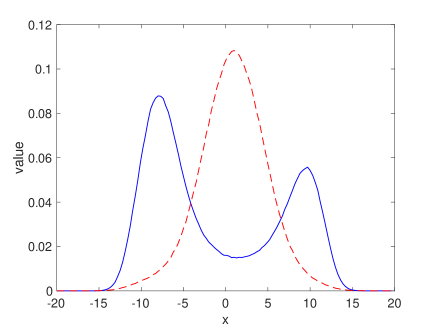
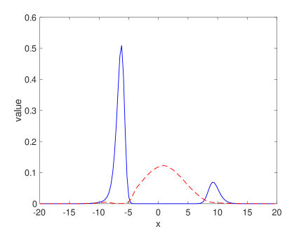
Figure 1. Nonsymmetric case: Densities of particle system (5) corresponding to the SKT population model (left) and particle system (3) (right) at time $t=2$. Solid blue line: species 1; Dashed red line: species 2.

7.2. Two species: symmetric case

We investigate the symmetric case by choosing $a_{11}=a_{22}=0$, $a_{12}=a_{21}=355$, and, as before, $\sigma_{1}=1$, $\sigma_{2}=2$. The initial data are chosen as in the previous example. In this example, we expect that cross-diffusion dominates self-diffusion. We present the approximate densities for different times in Figure 2. In both models, the species have the tendency to segregate. As expected, the segregation in the particle system (3) is stronger than in system (5) corresponding to the SKT model.

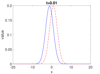
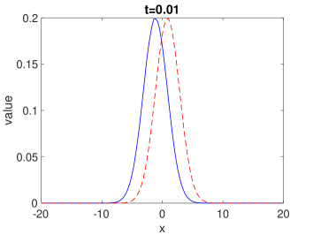
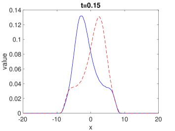
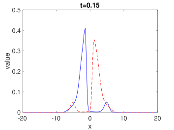
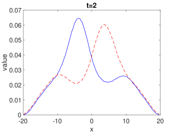
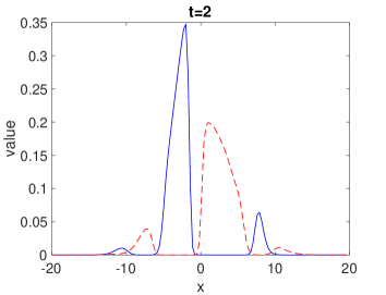
Figure 2. Symmetric case: Densities of particle system (5) corresponding to the SKT population model (left) and particle system (3) (right) for different times $t=0.01$, $0.15$, $2$. Solid blue line: species 1; dashed red line: species 2.

7.3. Three species

Our third numerical experiment illustrates the segregation behaviour in case of three interacting species with coefficients $\sigma_{1}=1$, $\sigma_{2}=2$, $\sigma_{3}=3$ and

$$(a_{ij})=\begin{pmatrix}0&355&355\\ 25&0&25\\ 355&0&0\end{pmatrix}.$$

Similar as in the two-species case, the initial data are overlapping normal distributions with means $-1$, 2, and $-3$, respectively, and variance 2. The approximate densities at $t=2$ are shown in Figure 3. We observe that the approximate densities of particle model (3) show a much clearer component-wise segregation behavior than the stochastic particle model (5), which corresponds to the SKT system, where the diffusion effects are much stronger. This may be explained by the fact that, on the PDE level, the gradient-flow structure of model (2) can be written species-wise, whereas the SKT model (1) (with $f(x)=x$) only posseses a vector-valued gradient-flow structure.

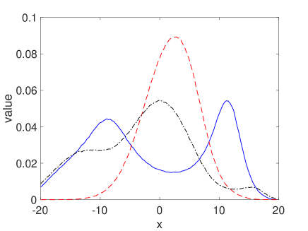
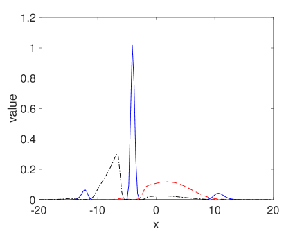
Figure 3. Three-species case: Densities of particle system (5) corresponding to the SKT population model (left) and particle system (3) (right) at time $t=2$. Solid blue line: species 1; dashed red line: species 2; dash-dotted black line: species 3.

7.4. Cubic nonlinearity

For our last experiment, we compare the numerical results for the cubic nonlinearity $f(s)=s^{3}$ with the linear case imposed in the previous examples. The parameters are the same as in Section 7.2. The numerical simulations are performed without using approximating functions $f_{\eta}$. This may be justified by the fact that the simulations deal with (relatively) small time scales and with compactly supported initial data. We observe in Figure 4 that the cubic nonlinearity causes more clustering than the linear case $f(s)=s$. The simulations suggests that in the cubic case, diffusion happens on a faster time scale than segregation, while in the linear case, the particles diffuse slower and hence they form bigger but fewer clusters.

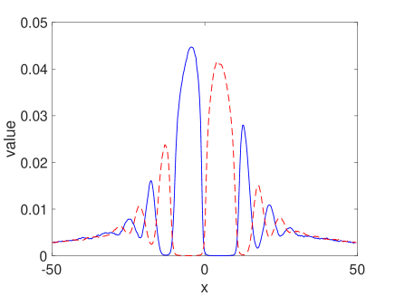
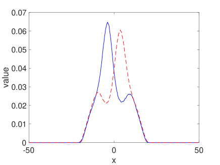
Figure 4. Densities of particle system (5) corresponding to the SKT population model with $f(s)=s^{3}$ (left) and $f(s)=s$ (right) at time $t=2$. Solid blue line: species 1; dashed red line: species 2. The right figure is the same as in Figure 2 (bottom right) but with the range $x=-50,\ldots,50$.

Appendix A Auxiliary results

For the convenience of the reader, we recall some well-known estimates used in this paper.

Lemma 11 (Young’s convolution inequality, [19, Formula (7), page 107]).

Let $1\leq p,q,r$ $\leq\infty$ be such that $1/p+1/q=1+1/r$ and let $f\in L^{p}({\mathbb{R}}^{d})$, $g\in L^{q}({\mathbb{R}}^{d})$. Then $f*g\in L^{r}({\mathbb{R}}^{d})$ and

$$\|f*g\|_{L^{r}({\mathbb{R}}^{d})}\leq\|f\|_{L^{p}({\mathbb{R}}^{d})}\|g\|_{L^{q}({\mathbb{R}}^{d})}.$$

Lemma 12 (Moser-type estimate I, [20, Prop. 2.1(A)]).

Let $s\in{\mathbb{N}}$ and $\alpha\in{\mathbb{N}}_{0}^{n}$ with $|\alpha|=s$. Then there exists a constant $C>0$ such that for all $f$, $g\in H^{s}({\mathbb{R}}^{d})\cap L^{\infty}({\mathbb{R}}^{d})$,

$$\|D^{\alpha}(fg)\|_{L^{2}({\mathbb{R}}^{d})}\leq C\big{(}\|f\|_{L^{\infty}({\mathbb{R}}^{d})}\|D^{s}g\|_{L^{2}({\mathbb{R}}^{d})}+\|D^{s}f\|_{L^{2}({\mathbb{R}}^{d})}\|g\|_{L^{\infty}({\mathbb{R}}^{d})}\big{)}.$$

Lemma 13 (Moser-type estimate II, [20, Prop. 2.1(C)]).

Let $s\in{\mathbb{N}}$ and $\alpha\in{\mathbb{N}}_{0}^{n}$ with $|\alpha|=s$. Then there exists a constant $C>0$ such that for smooth $g:{\mathbb{R}}\to{\mathbb{R}}$ and $u\in H^{s}({\mathbb{R}}^{d})\cap L^{\infty}({\mathbb{R}}^{d})$,

$$\|D^{\alpha}g(u)\|_{L^{2}({\mathbb{R}}^{d})}\leq C\|g^{\prime}\|_{C^{s-1}({\mathbb{R}})}\|u\|_{L^{\infty}({\mathbb{R}}^{d})}^{s-1}\|D^{\alpha}u\|_{L^{2}({\mathbb{R}}^{d})}.$$

Lemma 14 (Moser-type commutator inequality, [20, Prop. 2.1(B)]).

Let $s\in{\mathbb{N}}$ and $\alpha\in{\mathbb{N}}_{0}^{n}$ with $|\alpha|=s$. Then there exists $C>0$ such that for all $f\in H^{s}({\mathbb{R}}^{d})\cap W^{1,\infty}({\mathbb{R}}^{d})$ and $g\in H^{s-1}({\mathbb{R}}^{d})\cap L^{\infty}({\mathbb{R}}^{d})$,

$$\|D^{\alpha}(fg)-fD^{\alpha}(g)\|_{L^{2}({\mathbb{R}}^{d})}\leq C\big{(}\|Df\|_{L^{\infty}({\mathbb{R}}^{d})}\|D^{s-1}g\|_{L^{2}({\mathbb{R}}^{d})}+\|D^{s}f\|_{L^{2}({\mathbb{R}}^{d})}\|g\|_{L^{\infty}({\mathbb{R}}^{d})}\big{)},$$

where $D^{s}=\sum_{|\alpha|=s}D^{\alpha}$.