Detection of Local Mixing in Time-Series Data Using Permutation Entropy

Abstract

While it is tempting in experimental practice to seek as high a data rate as possible, oversampling can become an issue if one takes measurements too densely. These effects can take many forms, some of which are easy to detect: e.g., when the data sequence contains multiple copies of the same measured value. In other situations, as when there is mixing—in the measurement apparatus and/or the system itself—oversampling effects can be harder to detect. We propose a novel, model-free technique to detect local mixing in time series using an information-theoretic technique called permutation entropy. By varying the temporal resolution of the calculation and analyzing the patterns in the results, we can determine whether the data are mixed locally, and on what scale. This can be used by practitioners to choose appropriate lower bounds on scales at which to measure or report data. After validating this technique on several synthetic examples, we demonstrate its effectiveness on data from a chemistry experiment, methane records from Mauna Loa, and an Antarctic ice core.

I Introduction

In many fields of science, data are measured in gas or fluid states where local mixing occurs: in measurement chambers and laboratory piping, for instance. This can artificially interchange information between neighboring data points and thereby obfuscate the results. Similar effects can also be at work in the system under study: e.g., diffusion of isotopes in an ice sheet, which mixes climate data from successive years. In the face of these challenges, choosing an appropriate interval at which to measure, analyze, or report the data is often an imperfect balance between time, money, laboratory capabilities, and scientific need. Frequently, educated guesses are the only way to make these critical choices.

In this paper, we describe a novel technique to detect local mixing in a data set: not only whether or not it is present, but also (if so) on what scale. This gives practitioners a way to know precisely where to draw the line, in terms of sampling the system and reporting the data. Critically, our approach is model free, providing results without any need for domain-specific knowledge. The technique is based on a method called permutation entropy, which provides an estimate of the rate at which new information is produced in a data sequence: in effect, a measure of predictability. By varying the “stride” of this calculation, we can detect whether or not the data bear the scars of mixing. The underlying idea is as follows: for most time series, predictability tends to decrease as one extends the horizon, so permutation entropy will generally increase with the stride of the calculation because the data points involved span wider and wider temporal ranges. If successive data points are measured on a smaller scale than the mixing scales that are inherent in the data, though, each measurement is essentially a single draw from a local distribution composed of the data points in its local neighborhood. By definition, this added randomness will raise the entropy rate. Reversal of the normal pattern of the relationship between the stride of the calculation and the permutation entropy values, then, is an effective way to detect local mixing. Used in tandem with judicious bin averaging, this method also allows one to detect the scale of those mixing effects and adjust one’s procedures accordingly.

In Section II, we describe the techniques involved in our approach, beginning with some background on permutation entropy and describing the metric that we have developed to capture the effects described in the previous paragraph. We validate our technique using two synthetic examples (Sections III.1 and III.2) and explore its utility in the context of three real-world time-series data sets: one from a chemistry experiment involving gas mixtures (Section III.3), a second from an Antarctic ice core (Section III.4), and a third from the Mauna Loa methane records (Section III.5). We discuss these results and their implications in Section IV and conclude, with some thoughts about broader applications and future directions, in Section V.

II Materials and Methods

II.1 Permutation Entropy

Permutation entropy [1] is a method for estimating the Shannon entropy rate[2] of an arbitrary time-series data set. The calculation focuses on the local relationships among a sequence of points by mapping their values to an ordering of the same length. The three-point sequence $[7,3,11]$, for instance, would map to the ordering $[1,0,2]$ because $3<7<11$. The statistics of these ordinal sequences or permutations are calculated as follows. Let $|\cdot|$ denote set cardinality and Ord define a function that calculates the ordering of a given sequence of length $\ell$, as in the $\ell=3$ example above. Additionally, define a time series as the sequence $(x_{i})_{i\in I_{N}}$, where the index set is $I_{N}=\{k\in\mathbb{N}\setminus\{0\}\;|\;k\leq N\}$. Then the probability of the appearance in the time series of $\ell$-sequences of data points whose values map to a specific ordering $\pi$ can be estimated by

$$\mathrm{Pr}[\pi] =\frac{|\{n\in I_{N-\ell+1}\;|\;\texttt{Ord}(x_{n},x_{n+1},...,x_{n+\ell-1})=\pi\}|}{N-\ell+1}.$$ (1)

By calculating the probability of each of the $\ell!$ orderings across the whole time series, one constructs the permutation entropy or $PE$:

$$PE =-\frac{1}{\log\ell!}\sum_{\pi}\mathrm{Pr}[\pi]\log\mathrm{Pr}[\pi].$$ (2)

This is an estimate of the average rate at which new information appears in a time series per observation[1]. With the $1/\log\ell!$ normalization, its values range from 0 to 1. If $PE$ is low, the observations, on average, contain a significant amount of information about the past. This is the case for the sine wave in the top panel of Figure 1 where $PE\approx 0.012$.

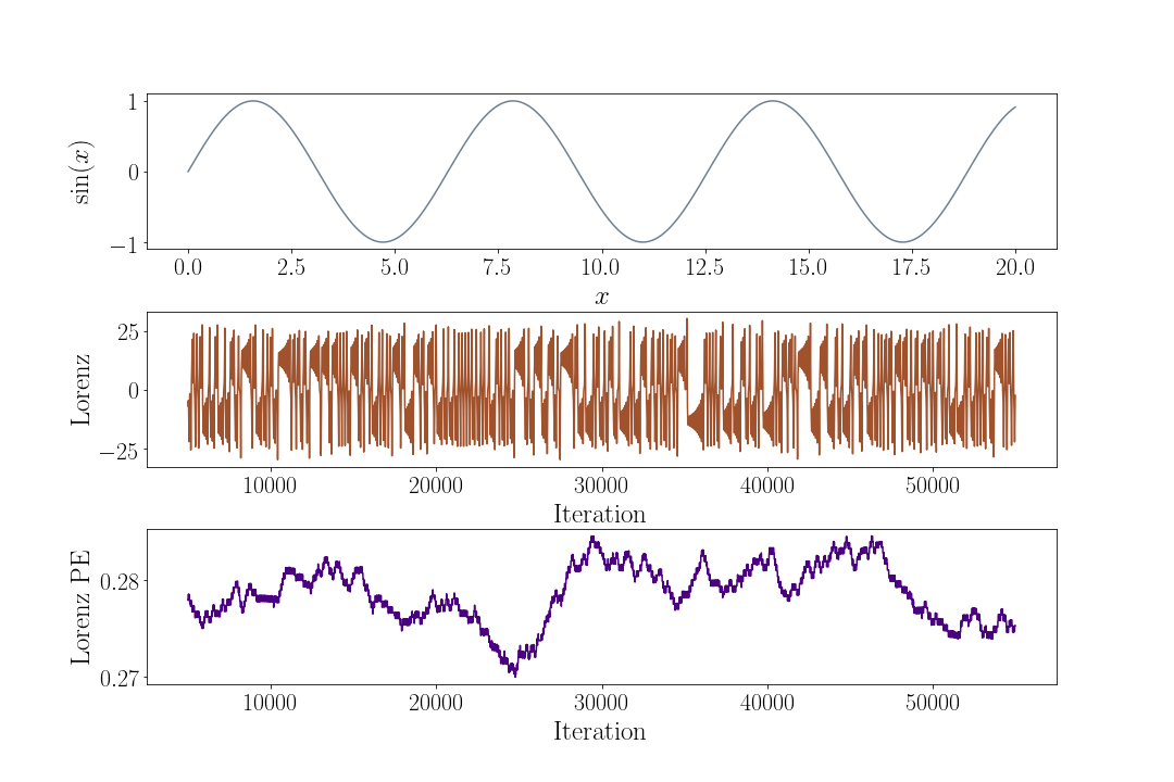
Figure 1: Demonstration signals Top: sinusoidal signal. Middle: a short segment of a chaotic signal from the Lorenz system. Bottom: permutation entropy of the Lorenz time series in the middle panel.

If $PE$ is high, on the other hand, most of the information in each observation is new. As such, this has been shown to correlate with predictability [3, 4, 5]. This is the case for the time series in the middle panel of Figure 1 from the canonical Lorenz system, described at more length later in this paper, where $PE\approx 0.28$, reflecting the limited predictability that is associated with deterministic chaos. If the signal were wholly random, the $PE$ would be 1. The value of the $PE$ is a function of the subsequence length $\ell$, of course; please see [7, 3, 8] for more discussion of this parameter and its implications.

As defined above, $PE$ captures the permutation entropy of an entire data set in the form of a single value. One can also perform this calculation in a sliding window across a time series to increase the temporal resolution of the results. This is a good idea, for example, if the dynamics of the system at hand are complex or nonstationary. In this variant of the calculation, each $PE$ value captures the statistics of the orderings in a window around the associated time point.

As shown in the bottom panel of Figure 1, this windowed analysis brings out subtle changes in the predictability of the Lorenz time series in the middle panel as it moves through different regimes in its behavior. However, it does introduce another free parameter into the calculation; see [9, 10] for discussion of the associated choices and issues.

All of the calculations reported in this paper use $\ell=4$ and $w=5000$, the former chosen via a careful persistence analysis that seeks stabilization of the results with variations in this parameter, and the latter as dictated by the formulas in [4, 11, 8, 12]. In a window of this length, each permutation of length four will have approximately 200 opportunities to appear at least once, which should be enough to rule out any forbidden ordinals[12].

II.2 Permutation entropy at varying temporal resolutions

The examples and equations in the previous section assume that one always works with ordinal permutations that are constructed from the values of successive points in a time series. It can also be useful to coarsen the grain of this procedure using $\tau$-separated points instead, thereby changing the temporal resolution of the calculation. This variant of the $PE$ technique, which was introduced in [9], requires a few modifications to the first step in the calculations. Specifically, Equation (1) becomes

$$\mathrm{Pr}[\pi] =\frac{|\{n\in I_{N-(\ell+1)\tau}\;|\;\texttt{Ord}(x_{n},x_{n+\tau},...,x_{n+(\ell-1)\tau})=\pi\}|}{N-(\ell+1)\tau}$$ (3)

where $\tau$ defines the spacing between the points in the time series that are used to construct the $\ell$-element ordinal permutations. With $\tau=2$, for instance, the first permutation constructed from the sequence $[1,4,6,2,5,3]$ would be $[0,2,1]$ because $1<5<6$.

The spacing parameter $\tau$ is the focus of the work reported here, and the central point of leverage for our technique. Because this parameter controls the “stride” of the calculation, changing its value allows one to understand the information dynamics of the system at different resolutions. This reveals some interesting patterns: persistence of features in $PE$ results across a range of $\tau$ values, for instance, indicates an effect in the underlying signal that spans multiple time scales. And in a wide range of data sets, we have observed that increasing the $\tau$ value generally raises the $PE$ curves. These data sets include a number of classic chaotic systems, two of which are used as examples later in this paper, as well as transient deterministic dynamics (e.g., the examples used in [9]), various paleoclimate records (e.g., [10, 13]), various one-second and one-minute financial price datasets, computer performance data from the experiments reported in [14, 15], and experimental data from a driven damped pendulum, which are available at [16]. Figure 2(a) demonstrates this in the context of the Lorenz signal from Figure 1.

(a)

(b)

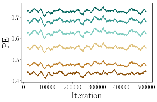
(c)

Figure 2: Lorenz permutation entropy. (a) Permutation entropy ($PE$) of the full version of the Lorenz signal from the middle panel of Figure 1, calculated with a range of values of $\tau$, the spacing between data points used to construct the permutations. (The trace in the bottom panel of Figure 1 is a short segment of the $\tau=1$ trace here.) Note the pattern of increasing $PE$ with $\tau$: i.e., the $\tau=a$ trace is higher than the $\tau=b$ trace for $a>b$. (b) If local mixing effects are artificially added to the same signal, the ordering of the $PE$ traces is reversed. (c) A simple bin averaging operation removes the local-mixing effects, restoring the normal order of the traces.

Note that the values of the permutation entropy increase monotonically with $\tau$. This simply reflects decreasing predictability over the longer time span sampled by each permutation. When there is local mixing in a time series, though, that reasoning no longer applies. Rather, because the data points used to construct individual permutations are measured on a smaller scale than the mixing scales that are inherent in the data, each element of those permutations is essentially a single draw from a local distribution composed of the data points in the neighborhood of each individual measurement. By definition, this added randomness will raise the $PE$. As $\tau$ increases, though, the points used to generate the orderings will spread out across those local distributions. When that point spacing exceeds the local distribution width—i.e., the largest mixing scale at work in the data—the extrinsic $PE$ increase [3] caused by that mixing will be reduced and eventually eliminated. The schematic in Figure 3 illustrates the mechanism underlying this effect.

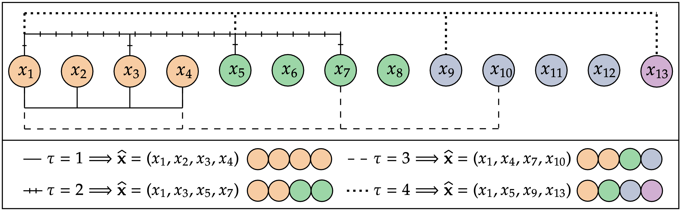
Figure 3: Mixing and permutation entropy. If the values of neighboring points are not independent and the $\tau$ value is small, then the points used to construct each permutation are effectively drawn from a single local distribution, schematized here with different colors. In this case, even though the underlying data may be deterministic, the relationships of these draws will be random and the permutation entropy will be artificially high. Higher $\tau$ values widen the span of the calculation beyond the spread of the local distributions, thereby mitigating this effect.

The takeaway here is that, when local mixing is at work in a data set, its $PE$ will not increase monotonically with $\tau$. Rather, the vertical ordering of the $PE$ curves in a plot like the ones in Figure 2 will be reversed, with the low-$\tau$ traces at the top and the high-$\tau$ traces at the bottom: the opposite of what we expect for a deterministic system. This reversal is not only a clear indicator of a specific issue in the data. With some additional experimentation, as described in Section II.4, this effect can actually bring out the scale of the mixing. First, though, we need a formal metric for assessing the relationships between permutation entropy curves calculated with different values of $\tau$.

II.3 Reversal Metric

The purely monotone nature of the vertical orderings of the different $PE$ traces in Figure 2 persists across the entire span of the time series, but that is not always the case; for some data sets, the traces will touch, or even cross, at different points in the time series. In order to assess the overall form of these patterns, what we want is a measure of how close this vertical ordering is to a purely monotone-increasing or monotone-decreasing pattern at different points in the time series. To quantify this formally, we develop the following metric. Let $\tau_{min}$ and $\tau_{max}$ denote the smallest and largest values of $\tau$ used in the $PE$ calculation. Additionally, let $\mathbf{v}_{i}$ denote the vector of monotone-increasing values of $\tau$:

$$\mathbf{v}_{i} =\begin{bmatrix}\tau_{min}&\tau_{min+1}&...&\tau_{max}\end{bmatrix}^{T}$$

If $\tau_{min}=1$ and $\tau_{max}=6$, for instance, this vector would be:

$$\mathbf{v}_{i} =\begin{bmatrix}1&2&3&4&5&6\end{bmatrix}^{T}$$

We construct a focal $\tau$-sequence vector, $\mathbf{v}$, that captures the ordering of the values of $PE$ at a given time $n$. (For the example in Figure 2, $\mathbf{v}=[1\;2\;3\;4\;5\;6]^{T}\;\forall\;n$.) We define the reversal metric $\mathcal{R}$ as the distance between this focal $\tau$-sequence vector and the purely monotone-increasing vector $\mathbf{v}_{i}$:

$$\mathcal{R}(\mathbf{v})=||\mathbf{v}-\mathbf{v}_{i}||/\lambda$$ (4)

where $\mathbf{v}\in\mathcal{S}_{\tau_{\max}}$, the set of permutations of order $\tau_{max}$, and $||\cdot||$ denotes the L1 norm. The scaling term $\lambda$, which is defined as

$$\lambda=\max_{\mathbf{y}}||\mathbf{y}-\mathbf{v_{i}}||$$ (5)

with $\mathbf{y}\in\mathcal{S}_{\tau_{max}}$, normalizes the value of $\mathcal{R}$ to run from 0 to 1, where 0 indicates perfect monotone-increasing order of the different $PE$ curves with $\tau$. This is the case for every time point in Figure 2(a). $\mathcal{R}=1$, on the other hand, indicates perfect monotone-decreasing order—as in Figure 2(b), where local-mixing effects have been added to the Lorenz signal via the procedure described in the following section. One can average these pointwise values of $\mathcal{R}$ across the time series, or over subsequences of it, in order to assess the overall reversal pattern in the corresponding span. In the examples in Figure 2(a) and (b), that average value $\overline{\mathcal{R}}$ is identical for all subsequences of the data. If the reversal patterns vary across the time series, though, that will not be the case—as will be shown in Section III.5.

The way of measuring distance that is encoded in Equation (4), which is a normalized version of Spearman’s footrule [17, 18], is more appropriate in our application than the Kendall-$\tau$ distance [19, 18]—which is essentially the number of pairs on which the relative order of two permutations disagrees—because a reversal of, say, the $\tau=1$ and $\tau=6$ traces is more meaningful than a reversal of the $\tau=3$ and $\tau=4$ traces because of the time scales involved. Other choices are of course possible for the form of this metric, as discussed in Section IV.

II.4 Data Manipulation Techniques

To validate our conjectures about the effect of mixing on the $\tau$ orderings of $PE$ traces, we perform a number of tests using synthetic time-series data sets $\mathbf{x}=(x_{n})_{n\in I_{N}}$ from well-known dynamical systems, manipulating them in order to create ansatzes that replicate the effects of mixing on those data: specifically, how it causes the interchange of information within some mixing window that includes $k$ points before and after each measurement. To do this, we create a local normal distribution at each point $\mathbf{x}_{n}$ whose mean and variance are calculated from the points in that mixing window around that point. To produce the corresponding point of the ansatz, $\hat{\mathbf{x}}_{n}$, we make a random draw from that distribution:

$$\hat{\mathbf{x}}_{n}{\sim}\textrm{Normal}(\mu_{n},\sigma_{n}^{2})$$

where $\mu_{n}$ and $\sigma_{n}$ are the mean and standard deviation of the points of $\mathbf{x}$ in the window:

$$[\mathbf{x}_{n-k},\dots,\mathbf{x}_{n},\dots,\mathbf{x}_{n+k}]$$

This is a comparatively simple model of the effects of mixing on a series of data points; it does not capture long-range effects, for instance. But for a wide range of experimental situations, this is a useful approximation.

In the following section, we also make use of binned averaging, where one uses groups of $j$ consecutive points of a time series $\mathbf{y}$ to create the elements of a new series $\overline{\mathbf{y}}$:

$$\overline{\mathbf{y}}_{n} =\left(\frac{y_{(n-1)j+1}+y_{(n-1)j+2}+...+y_{nj}}{j}\right)_{n\in I_{N/j}}$$ (6)

Note that this is not a rolling bin average; rather, the first point of $\overline{\mathbf{y}}$ is the average of the first $j$ points of $\mathbf{y}$, the second is the average of $[\mathbf{y}_{j+1}...\mathbf{y}_{2j}]$, and so on. This is intended to mimic what happens in experimental practice when $j$ successive points in a raw data set are averaged together—in the system, in the post processing, or in the laboratory apparatus. In the analyses that follow, this technique serves two purposes: as an extra validation step in the synthetic examples and as a diagnostic of mixing scales in the real-world data sets.

III Results

As validation and demonstration cases for our mixing-detection technique, we use two synthetic examples—classic systems from the field of nonlinear dynamics—and three real-world time-series data sets. The synthetic-data examples allow us to manipulate the time series, as described in Section II.4, in order to validate our reasoning about mixing and $\tau$ reversal. The experimental data sets—chemical sensor measurements from a gas mixing experiment, water-isotope data from an Antarctic ice core, measured by a spectrometer, and atmospheric methane from the Global Monitoring Laboratory observatory on Mauna Loa, Hawai’i—provide a first view into the utility of this technique in real-world settings. Figure 4 shows a data sample from each of these time series.

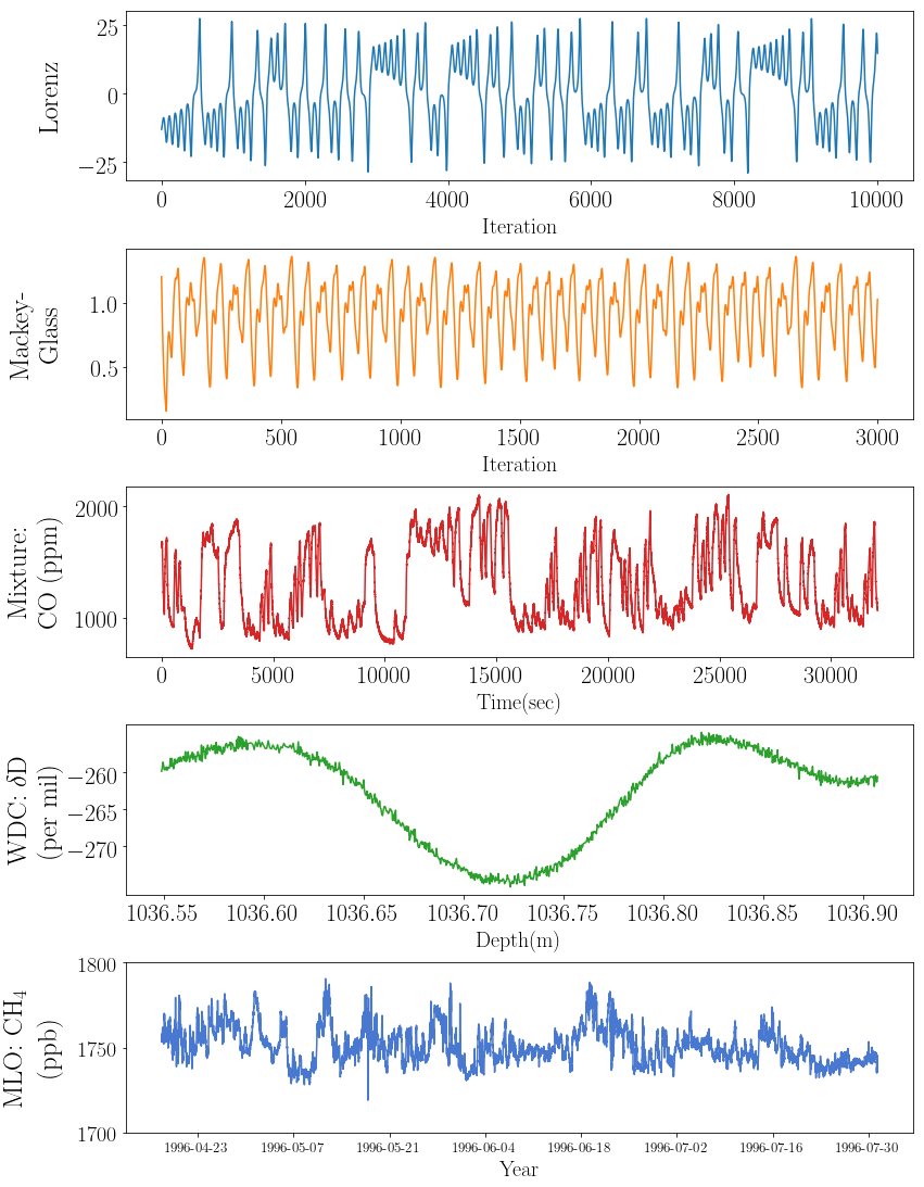
Figure 4: Data sample. A sample from each of the four time-series data sets used as examples in this paper: the classic Lorenz and Mackey-Glass systems from nonlinear dynamics, chemical sensor data from a gas-mixing experiment, water-isotope data from an Antarctic ice core (WDC), and atmospheric methane records from Mauna Loa (MLO).

III.1 Lorenz system

The Lorenz system [20] is defined by the following ordinary differential equations:

$$\dot{x} =a(y-x)$$

$$\dot{y} =x(r-z)-y$$

$$\dot{z} =xy-bz$$

To create a synthetic data set from this system, we choose $a=16,\;b=4,$ and $r=45$—parameter values that are known to produce chaotic behavior—and integrate the ODEs using a $4^{th}$ order Runge-Kutta method for 500,000 steps with a step size of $h=0.005$, starting from the initial condition $[x_{0},y_{0},z_{0}]=[-13,-12,52]$. The $x$ coordinate of this trajectory—the first 55,000 points of which are shown in the top trace in Figure 4—is the baseline time series $\mathbf{x}$ for the set of tests reported in this section.

Using the process described in Section II.4, we manipulate this high-resolution trajectory in order to replicate the effects of local mixing in real experiments. The details are as follows. At each point $\mathbf{x}_{n}$ in the original time series, we calculate the mean and variance of the points in a window of width six, centered on that point (i.e., $[\mathbf{x}_{n-3}...\mathbf{x}_{n+3}]$) and then make a random draw from a normal distribution with those parameters to obtain the corresponding point of a new time series $\hat{\mathbf{x}}_{n}$. We choose a mixing window of width six for this first experiment because $\ell=3$ gives us points from many distributions for each $\tau$.

As discussed previously, this $\hat{\mathbf{x}}$ signal—whose $PE$ is shown Figure 2(b)—is an ansatz that is specifically designed to let us explore the effects of local mixing in a controlled experiment. As expected, the monotone-increasing vertical order that is apparent in the $PE$ traces calculated from the original time series is reversed by the local-mixing operation. The corresponding value of the reversal metric $\overline{\mathcal{R}}$, computed across the span of the $PE$ traces in Figure 2(b), is 1, reflecting the perfect monotone-decreasing order of those traces with $\tau$. (This would also be the case for $\overline{\mathcal{R}}$ computed across any subsequence of those traces, since the ordering is reversed everywhere: i.e., $\mathcal{R}=1\;\forall\;n$.) Note that the $PE$ values are higher than in Figure 2(a). This simply reflects the additional randomness introduced by the local mixing operation. Careful examination shows that that effect decreases with $\tau$: the $\tau=6$ trace in Figure 2(b), for instance, has roughly the same mean value as in Figure 2(a), but the movement in the smaller-$\tau$ traces is comparatively larger. This is due to the mitigation of the mixing effects that occurs with larger $\tau$ values.

Our original conjecture was that one could effectively remove the added local mixing effects in $\hat{\mathbf{x}}$ by taking a binned average of that signal using the technique described in Section II.4, with a bin size $j$ roughly equal to the size of the mixing window used in the creation of that ansatz. This conjecture can be easily tested using the ansatz signal, as binning at that scale should “undo” the $\tau$ reversal produced by that synthetic mixing manipulation, thereby restoring the normal ordering. We propose the following heuristic for choosing the value of $j$ to remove the local-mixing effects: bin-average the time series using varying bin sizes $j$, calculating $\overline{\mathcal{R}}$ across the span of the time series at each one, and choose the first bin size where $\overline{\mathcal{R}}$ goes to zero; if $\overline{\mathcal{R}}$ never reaches zero, choose the first minimum of this curve. Figure 5(a) shows such a plot for the Lorenz ansatz.

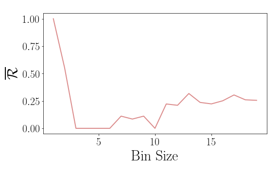
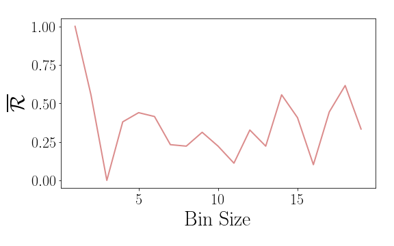
(a)                                                                 (b)

Figure 5: Bin size and mixing scales. Plots of $\overline{\mathcal{R}}$ versus bin size for the (a) Lorenz and (b) Mackey-Glass examples.

As the bin size increases, the curves start reordering themselves, with $\overline{\mathcal{R}}$ reaching zero at $j=3$. Beyond that, the ordering shifts because of the complicated relationships between the different timescales of the analysis ($\tau$, $\ell$, the mixing window, and the bin size). The $PE$ traces in Figure 2(c), computed from the Lorenz ansatz $\hat{\mathbf{x}}$ binned with $j=3$, are in clear monotone-increasing order with $\tau$, consistent with the $\overline{\mathcal{R}}$ value of 0.

These results confirm that the binning process—a data-manipulation step that manipulates the ansatz to eliminate the simulated effects of local mixing—does indeed restore the normal ordering. Note that the bin size indicated by our heuristic is smaller than the local mixing window that was used to create the ansatz, so our original conjecture was off by a scale factor. This is discussed further below. Note, too, that the binning operation does not restore the exact form of the original traces in Figure 2(a), just their ordering. The $PE$ values in Figure 2(c) are higher because of the residual effects of the added mixing. The difference in the smoothness of the traces in these two images is partially due to the altered window size—from the reduction in the number of points in the $\overline{\mathbf{x}}$ signal—as well as the difference in the scales of the images.

This series of experiments validates the conjecture that, when local mixing occurs in a data set, high sampling rates can lead to reversal of the normal ordering of permutation entropy with changing $\tau$. This observation is a potentially useful way to detect the presence of local mixing in experimental data. The bin size that restores the correct ordering is an indicator of the scale of the effect, and that size can be chosen from a curve like the one in Figure 5(a). Our experiments show that this claim holds for different mixing windows, as well as for different $w$ and $\ell$ values. In all cases, that bin size is smaller than, but on the same order as, the mixing window used in the creation of the ansatz. The implications of this, for experimental practice, are that this operation effectively identifies the order of magnitude of the mixing scale in the data, though not its specific value.

These results are encouraging, but this is only one system, and a low-dimensional one at that. In the following section, we replicate these steps with a more-complicated dynamical system.

III.2 Mackey-Glass System

The Mackey-Glass system [22] is described by a delay-differential equation of the following form:

$$\dot{x} =\beta\frac{x(t-t_{0})}{1+x(t-t_{0})^{q}}-\gamma x,\quad\gamma,\beta,q>0.$$ (7)

The delay here makes this system effectively infinite dimensional, even though there is only a single state variable. Like the Lorenz system, Mackey-Glass is known to exhibit deterministic chaos for some values of the parameters $\gamma,\beta,t_{0}\textrm{ and }q$. Using $\beta=0.2,\gamma=0.1,t_{0}=17,\textrm{ and }q=10$, we integrate Equation (7) with the same Runge-Kutta solver for $1.5\times 10^{6}$ steps from an initial state of $x=1.2$ using a step size of $0.1$ to obtain our test data $\mathbf{x}$. The first 3000 points of this time series are shown as the second trace in Figure 4.

The procedure for exploring $\tau$ reversal in this example is exactly the same as in the Lorenz system in the previous section. Figure 6 shows $PE$ traces of the ${\mathbf{x}}$, $\hat{\mathbf{x}}$ and $\overline{\mathbf{x}}$ signals.

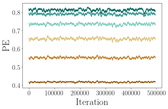
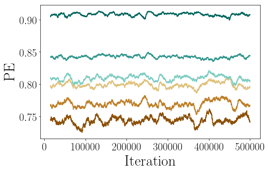
(a)                                   (b)                                   (c)

Figure 6: Reversal results in the Mackey-Glass system. $PE$ traces from the Mackey-Glass system with $1\leq\tau\leq 6$ for (a) the original time series (b) with added local-mixing effects (c) after a bin-averaging operation was applied to remove those effects.

Figure 6(a) demonstrates normal, monotone-increasing order, with $\mathcal{R}=0$ at all time points and a corresponding value of $\overline{\mathcal{R}}=0$ computed across the span of the time series. For the locally mixed ansatz $\hat{\mathbf{x}}$ in Figure 6(b), which was created with a mixing window of eight, the order is reversed and $\overline{\mathcal{R}}=1$. As before, bin averaging with a bin size chosen at the first minimum of the $\overline{\mathcal{R}}$ versus $j$ curve for this signal (Figure 5(b)) completely restores the monotone-increasing order of the $PE$ traces, as shown in Figure 6(c). Again, the form of these results persists for different mixing windows, as well as for different values of the parameters of the $PE$ calculations. And as in the Lorenz examples, the bin size needed to fully restore the normal ordering is always smaller than, but on the same order as, the mixing window used in the creation of the ansatz. In other words, this value provides a useful litmus test for the scale of that effect, even if it does not indicate the exact value.

These results reaffirm the overall relationship between local mixing effects and $\tau$ reversal. Next, we move to data from physical experiments.

III.3 Gas Mixture Data

As a first real-world demonstration case for these techniques, we use a data set from the UCI Machine Learning repository [23] that was produced during a chemistry experiment involving gas mixing. The values in this time series were measured by a sensor measuring carbon monoxide and ethylene mixtures in air under changing concentration conditions [24]. We focus on the $9^{th}$ sensor in the array, a Firago TGS-2600 instrument that reports particle concentrations in PPM. These data have an extremely high background noise level, which raises all the $PE$ curves to the top of their ranges and scrambles their order, so we first perform a filtering step. The third plot in Figure 4 shows 30,000 data points from the resulting time series, which is spaced at 0.25 sec. See the Supplementary Material for the full trace.

$PE$ traces calculated from this time series demonstrate reversed $\tau$ ordering across the entire span of the data set, as shown in the plot in Figure 7(a), with $\overline{\mathcal{R}}=1$.

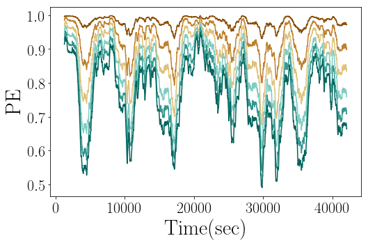
(a) Gas Mixture – Raw

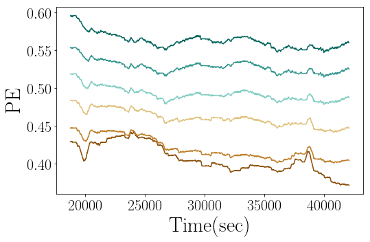
(b) Gas Mixture – Binned with $j=15$

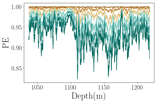
(c) WDC – Raw

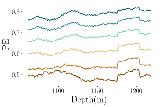
(d) WDC – Binned with $j=15$

(e) Mauna Loa – Raw

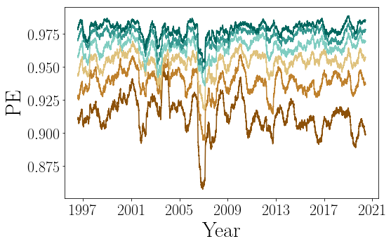
(f) Mauna Loa – Binned with $j=4$

Figure 7: Reversal results in experimental data sets. From top to bottom: $PE$ traces for the gas mixture, WAIS Divide, and Mauna Loa data. In all cases, the images in the left and right columns show the calculations for the raw and bin-averaged data, respectively. The traces in the latter are temporally offset by the width of the binning window times the width of the $PE$ calculation window. (This offset is essentially invisible in the WDC data because of the number of data points in the time series.)

This suggests that local mixing was at work during the collection of these data: in the chamber, perhaps, or the compartment in the sensor. To ascertain whether this was indeed the case, we perform a bin averaging step on the data—as in the synthetic examples in the previous sections—and observe how that operation affects the ordering of the $PE$ curves. And as in those previous examples, we can repeat this analysis using varying bin sizes in order to estimate the scale of the mixing effects.

In this example, the results of that procedure are quite clear, though the shape of the $\overline{\mathcal{R}}$ versus bin size curve is somewhat different than in our synthetic examples; see Figure 8(a).

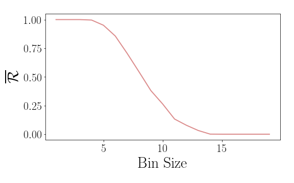
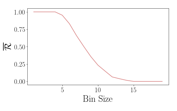
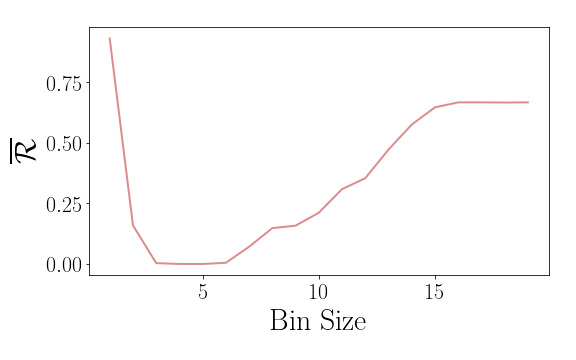
(a)                                   (b)                                   (c)

Figure 8: $\overline{\mathcal{R}}$ as a function of bin size (a) gas mixture (b) WAIS Divide and (c) Mauna Loa Methane

As before, the $PE$ traces move towards normal ordering as the bin size increases, but $\overline{\mathcal{R}}$ then reaches a broad minimum that begins at $j=15$ and extends to $j=54$ (not shown). Figure 7(b) shows that the $PE$ traces for data bin-averaged with $j=15$—i.e., 3.75 seconds—are in fully normal order. These results not only confirm that local mixing is at work in the raw data, but also suggest a scale for those effects. This, in turn, has implications for the resolution at which these data should be reported.

III.4 Antarctic Ice-Core Data

Water isotopes in ice cores, which are viewed as climate proxies [26], can be measured at very high resolution in modern continuous flow analysis (CFA) equipment [27]. During this process, the ice is continuously melted and then piped through tubing into an optical spectrometer that measures the ratios of heavy to normal variants of oxygen and hydrogen isotopes in the ice. The CFA apparatus in the Stable Isotope Laboratory at the Institute for Arctic and Alpine Research at the University of Colorado can perform these measurements at sub-millimeter resolution. Basic fluid dynamics makes mixing inevitable in the different stages of this analysis pipeline; see [27] for discussion of the associated issues. Diffusion causes these isotopes to mix in the ice sheet as well, before the samples reach the laboratory, so there are at least two potential sources of mixing in these data—perhaps with different scales.

The West Antarctic Ice Sheet Divide Core (WDC) is 3300m long, so a data set gathered from this core with sub-millimeter spacing contains many million points. Here, we focus on a short segment of that record: the ice from 1035.4 m–1368.2 m, which captures climate information from roughly 4500-6500 years ago [11, 28]. The fourth trace in Figure 4 shows a small segment of the hydrogen isotope ($\delta\text{D}$) data from this core; see the Supplementary Materials for the full trace. These data are reported in delta ($\delta$) notation relative to the baseline Vienna Standard Mean Ocean Water (VSMOW) and normalized to the Standard Light Antarctic Water (SLAP, $\delta\text{D}=-428.0$ ‰) scale. The $\delta$ value is determined by $\delta=1000(\rho_{sample}/\rho_{VSMOW}-1)$, where $\rho$ is the isotopic ratio D/H (i.e., ${}^{2}\text{H}/^{1}\text{H}$). Please see [10] for more details about these data. The sinusoidal pattern is a result of seasonal variability in temperature.

As is customary in this field, the raw, high-resolution data—0.3 mm spacing, in this data set—undergo a number of post-processing steps: removal of outliers, interpolation to fill gaps where data are missing, etc. The final step in the laboratory’s post-processing procedure involves a binned average of the data, with the bin scale explicitly chosen to reduce any mixing effects. In this case, the Stable Isotope lab used a bin size of 0.5 cm (i.e., 17 points at an 0.3 mm spacing) to construct the published version of this data, which is available at [28].

This provides a unique opportunity for our work: using permutation entropy, we can not only assess whether mixing was indeed at work in the raw data, but also potentially identify the associated scales, and even validate our results against expert judgment about those scales. To that end, we calculate $PE$ and $\overline{\mathcal{R}}$ for the raw 0.3 mm spaced data. Similarly to the gas mixture data in Section III.3, the higher-$\tau$ $PE$ traces are below the lower-$\tau$ traces across the full span of the data set; see Figure 7(c). The corresponding $\overline{\mathcal{R}}=1$ value reflects this consistent reversal of the normal monotone-increasing order across the entire time series. As in the gas-mixture example, this suggests that local mixing effects are present in those data. Note that $\tau$-reversal does not identify the mechanics of the effect, or its source. In this example, there are many potential culprits: the laboratory apparatus and the physics of the ice sheet, among other things. See Section IV for more discussion.

Note that we have moved to speaking of spatial scales and resolutions here—depths in the core—rather than temporal scales. Over this span of the WDC, there is a linear relationship between depth and age, with 0.5 cm of ice translating to 1/34th of a year of climate record, so these depthwise data can be viewed as time-series data. This would not be the case if we were using a longer span of the core—particularly one that extended to its deeper levels, where the nonlinearity of the age-depth relationship more strongly affects the temporal spacing of the data points.

To explore the mixing scales in this ice-core record, we again use bin averaging, computing $\overline{\mathcal{R}}$ from the raw 0.3 mm data, binned at a range of bin sizes. The shape of this curve, which is shown in Figure 8(b), is similar to the one for the gas-mixture data, reaching a broad minimum at $j=15$ with $\overline{\mathcal{R}}=0$. That is, bin-averaging the raw data using $j=15$ restores the normal order of the $PE$ traces; this is clearly visible in Figure 7(d). As before, this is an indication of the scale of the mixing effects that are present in the data. In this case, where we have expert judgment as a point of comparison, that scale can be corroborated. Recall that the laboratory used a bin size of 17 to construct the data to be reported on the U.S. Antarctic Program Data Center website, basing that choice on expert knowledge about the CFA apparatus. In other words, our technique not only matches expert reasoning about the data, but does so in a manner that is completely model-free, requiring no knowledge about the system that produced the data or the apparatus that was used to measure it.

This analysis brings out the effects of any local mixing process, of course—not just laboratory effects. Since the isotopes mix via diffusion in the ice sheet, there are also potential scientific implications of these results, as discussed further in Section IV.

III.5 Mauna Loa Methane Data

NOAA’s Global Monitoring Laboratory has been measuring atmospheric composition from Mauna Loa Observatory in Hawaii (altitude = 3397 m) at high temporal resolution for decades. Air is pumped continuously at $\approx 6L/min$ from two inlets 40 m above the surface to a manifold inside the laboratory where $\approx 100mL/min$ of the flows is fed to a calibrated analyzer that measures the abundance of atmospheric CH4 at fixed intervals [29]. Over the period on which we focus in this paper, two well-calibrated analysis methods were used. In both cases, the analyzer alternates between the two inlets. From 1996 to 9 April 2019, measurements were by gas chromatography with flame ionization detection (GC/FID) at 15 minute intervals, reported in ppb. For each measurement, a 10 mL (at STP) slug of air is injected into the GC/FID system every 15 minutes. The response of the detector is compared with bracketing measurements of standard to quantify $CH_{4}$. From 11 April 2019 to present, a Cavity Ring-Down Spectrometer (CRDS) was used. This instrument records nine 10-second averages of $CH_{4}$ every five minutes and averages them into a single “five-minute average” value, also reported in ppb. It is calibrated with a suite of standards every two weeks relative to a reference cylinder of natural air; this reference is measured once per hour during normal monitoring to track drift in the analyzer.

Because $PE$ calculations require data with a constant temporal spacing, we first downsampled the 5 min segment of the data to produce an 826,633 point time series at an even 15 minute spacing, beginning at 0007 on 1 January 1996 and ending at 2350 on 7 June 2020. We then scanned the data for missing or damaged values, replacing each of them with the last good value. The fourth plot in Figure 4 shows a 10,000-point segment of this record beginning in March of 1996; a plot of the full data set appears in the Supplementary Materials.

The ordering of the $PE$ traces of this important data set, which are shown in Figure 7(e), is more complex than in the previous two examples. The overall pattern is reversed, but not perfectly, with $\overline{\mathcal{R}}=0.907$, rather than 1.0, as in all of the previous examples. In other words, local mixing effects are almost certainly in play here, but the indication is not as clear as in the gas-mixture and ice-core examples, where $\mathcal{R}=1$ at every point in time (and $\overline{\mathcal{R}}=1$ for the whole span). Moreover, nonstationarity is obviously an issue: viz., the downward spikes in $PE$ values, especially at $\tau=1$ (e.g., in 2004), for instance, and the short regions where the $\tau$-ordering of the traces changes (e.g., in 2010 and from 2019-on). Some of these issues can be traced back to the data-cleaning and quality-control processes; many of the dips, for instance, correspond to regions where a large fraction of the data are missing or damaged. Replacing those points with the last good value effectively creates a constant signal which, by definition, obeys normal $\tau$ ordering. This is a well-known challenge in the permutation entropy literature: one that causes problems for all data-cleaning strategies, including ours [31, 32, 3].

As before, we can repeat the $\overline{\mathcal{R}}$ calculation for a range of bin sizes in order to confirm the presence of mixing and estimate the associated scale. In this case, as Figure 8(c) shows, the first minimum of $\overline{\mathcal{R}}$ falls at $j=4$. The $\overline{\mathcal{R}}$ value at this point is 0, indicating that a binning operation at a scale of one hour eliminates the local mixing effects. This is reflected in the ordering of the resulting traces, shown in Figure 7(f), which are in monotone-increasing order with $\tau$. Again, our results are in good alignment with standard practice in this field, which prescribes a one-hour reporting cadence. As in the gas-mixture and ice-core examples in the previous section, this has implications for both analysis and reporting. Unlike those examples, though, the curve in Figure 7(f) rises strongly for $j>5$. This behavior, which more closely resembles the two synthetic examples in Figure 5, is likely due to the time scales involved, in the systems and in the calculations—as well as to data limitations, which precluded a broader span on the horizontal axes of Figure 7(d) and (e).

When one suspects nonstationarities, it can be informative to perform a more-focused analysis: specifically, to compute $\overline{\mathcal{R}}$ over windows of the $PE$ traces, rather than over their entire temporal extent. Figure 9 shows the results of this calculation for the raw and binned MLO methane data that uses a window size of 5000 points.

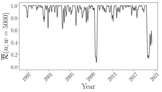
Figure 9: Windowed $\overline{\mathcal{R}}$ Analysis for the Mauna Loa data

This plot brings out the nonstationarities of the data very clearly. From 1996 through early 2019, $\overline{\mathcal{R}}$ oscillates between 1.0 and 0.7, with occasional drops to $\approx$0.6 and one even lower, in 2010. These results confirm that the mixing effects in this segment of the time series vary across the time series: the ordering of the curves is largely reversed across most of the span of the data, but the magnitude of that reversal varies with time. Many of these nonstationarities are due to the quality-control and data-cleaning processes, as described above. Between June 2009 and May 2010, for instance, at the time of the obvious spike in the middle of the curve, 5066 of the 31000 points were missing or damaged. Standard interpolation strategies for filling these gaps—a necessary step because $PE$ calculations require data that are evenly spaced in time—employ smooth functions: lines, curves, etc. Data spaced in this manner are inherently predictable, so the $PE$ values in the repaired spans will be low and the $\tau$ ordering will be monotone increasing, hence the drop in $\overline{\mathcal{R}}$. These effects are visible in $PE$ traces themselves—Figure 7(e) and the magnified views that appear in the Supplementary Materials, which zoom in on the time spans around 2000 and 2009—but they really stand out in the windowed $\overline{\mathcal{R}}$ plot in Figure 9. The same effects are also at work in many of the smaller dropouts in $\overline{\mathcal{R}}$: e.g., a temporary 10X increase in analyzer noise that occurred in June 2003, causing many of the points in this time span to be flagged during the quality-control process as suspicious, and therefore removed in our data-cleaning process.

One of the most interesting features of Figure 9 is the precipitous drop in $\overline{\mathcal{R}}$ in the spring of 2019. Recall that the Observatory switched from a gas chromatograph to a cavity ring-down spectrometer at 0155 on 11 April 2019, at the same time as the shift in measurement cadence. This newer instrument has a factor of 5 to 10 less short-term noise than the gas chromatograph that it replaced. Our metric detects this quite effectively from the raw data, not only flagging the timing of the change, but indicating clearly that the introduction of this new instrument significantly reduced the mixing effects in the data. This provides additional corroboration of the efficacy of our technique, and also has implications for the scientific analysis, as described in the following section.

IV Discussion

The synthetic-data experiments in Sections III.1 and III.2, which use ansatzes that are expressly designed to mimic the effects of local mixing, confirm our conjectures about $\tau$-reversal of $PE$ curves as an indicator of local mixing in a data set. In both cases, the $\overline{\mathcal{R}}$ metric shows that the monotone-increasing order of the $PE$ traces for the original data is reversed when information is artificially interchanged between neighboring data points. In both examples, a bin-averaging operation on these artificially mixed time series restores the normal order—as expected, since that operation compresses the distribution that is effectively created by that mixing down to its mean. The bin sizes required to accomplish this are on the same scale as, but somewhat smaller than, the width of the mixing window that we use to create the ansatzes. One can leverage this observation to estimate the mixing scale: specifically, when the $\overline{\mathcal{R}}$ value of the $PE$ curves reaches zero.

Applied in tandem with judicious bin averaging, this reversal metric has an even more powerful role in the examples in Sections III.3, III.4, and III.5, which involve data from real-world experiments. In all of these cases except a few spans of the Mauna Loa data, the $\tau$-reversal metric suggests that the resolution of these data sets was actually high enough that the raw data are essentially repeated draws from a distribution composed from the data in a local window around each point. Permutation entropy brings this out quite effectively, if one varies the $\tau$ parameter in the calculation and evaluates the ordering of those results. And even though this operation may not reveal the exact distribution of the mixing effects, it has important practical implications, as it gives an indication of the scales of those effects—not just their presence or absence. This can be used, together with expert knowledge and other data-analytic techniques, to select an appropriate lower bound on the interval at which one should analyze, or report, the data.

Departures from pure monotonicity in the $PE$ traces are a complex and interesting question. If $\overline{\mathcal{R}}$ does not reach zero for any bin size, for instance, one can choose the first minimum of a curve like the ones in Figure 5 or 8 to perform the binning, but that is not guaranteed to remove all of the mixing effects—especially if nonstationarities are involved, causing the mixing scales to vary across the data set. Deconvolving multiple nonstationary mixing processes would call for strategies far more sophisticated than simple binning at a fixed resolution across the whole time series. A formal solution to this would be a major challenge, given the complex nature of the nonlinear statistics that underpin permutation-entropy analyses. Nonetheless, a windowed $\overline{\mathcal{R}}$ analysis like the one shown in Figure 9 can help ascertain whether there are different regimes in the data, with different noise & mixing properties in each—as in the different segments of the Mauna Loa methane data, before and after the instrument change.

A major advantage of our technique is its model-free nature: it identifies the mixing scale regardless of the cause. This has disadvantages as well, though: if two mixing processes are at work, our analysis will bring out the larger one. If the scales are widely separated and one has very fine-grained data, it might be possible to extend this analysis to detect the different scales. This is a potential issue in the WDC data, where there are two known sources of mixing: diffusion of the isotopes in the ice sheet and fluid mixing in the laboratory analysis pipeline. Diffusion is a function of density, and density in a ice core is a function of depth, so the effects are not simple. Standard procedure in this laboratory is to use estimates of the accumulation rate and temperature to make an educated guess at the diffusion scale at each depth. In constructing the published data set from the raw data, the analysts chose a sample rate that exceeded that resolution—in effect, intentionally oversampling the data—and then selected a bin size that spaced the reported data points safely above their estimates of the mixing scales. If those estimates are good, this procedure will obviously make the two mixing scales (diffusion in the ice sheet and fluid dynamics in the laboratory apparatus) very similar, so we do not expect to be able to deconvolve these two effects from this data set.

Similarly, there are a number of different potential sources of the mixing effects in the Mauna Loa data. While the sample lines are unlikely to be at issue because the flow through them can be approximated as plug flow, there is noise in the analyzer. There are also known sources of organized natural variability in the study system itself, which span the time scales from days to decades:

1. Diurnal cycle related to local wind regime,

2. Synoptic scale variability occurring on time scales of weather fronts (a few days),

3. Seasonal cycle related to changing atmospheric loss process rate, and

4. Long-term trend related to imbalance between emissions and losses.

We did not find any correlation between $\overline{\mathcal{R}}$ and meteorological parameters, although Dlugokencky et al. [29] showed that, on average, the diurnal cycle in atmospheric $CH_{4}$ correlated with dew point, because both are impacted by daily cycling between upslope and downslope wind regimes. Of course, there could be convolved effects from multiple causes, but those would be difficult to study in isolation with a permutation-entropy analysis for the same reasons mentioned at the end of the previous paragraph.

The alignment between our results and scientific knowledge about the experimental situation is encouraging. The $\overline{\mathcal{R}}$ calculations also clearly bring out the timing, as well as the salutary effects, of the 2019 instrument change on Mauna Loa, for instance. In the ice core data, the $\overline{\mathcal{R}}$ metric revealed that a 15-point averaging window restored the normal order of the $PE$ traces, when the experts chose a 17-point window. Similarly, our method suggested a one-hour mixing window for the Mauna Loa data, which is exactly the cadence that is used in practice. In the data gathered by the newer instrument, the same strategy indicated a significant reduction in the mixing scales, corresponding to a 25-minute cadence.

While corroboration of the known properties of a new instrument is not that exciting, there can be unknown mechanisms at work in one’s data, leaving traces that are all but invisible to normal analysis techniques. Indeed, this was the driving force behind the creation of the WDC data set used for this work. After a permutation entropy analysis revealed noise introduced by the CRDS instrument that had been used to analyze this section of the ice core [11], the analysis was repeated using a newer instrument, removing the noise effects. Finally, the results of the analysis described in the previous sections not only corroborate the reasoning behind the approaches taken by the experts, but could also provide a more systematic way to figure out exactly how to squeeze as much information out of a study system as nature will allow. Note that this does not mean that data measured below the mixing scale are useless; indeed, one must sample below a scale in order to identify its lower boundary.

There are many avenues for extension of this work. The metric used in the pointwise $\tau$-reversal metric ($\mathcal{R}$) and the temporally aggregated nature of its average, $\overline{\mathcal{R}}$, have pros and cons. Recall that $\mathcal{R}$ is based solely on the L1 norm of the distance between the focal $\tau$-sequence vector $\mathbf{v}$ and the purely monotone vectors $\mathbf{v}_{i}$ and $\mathbf{v}_{d}$. While this is a sensible measure of an overall pattern of monotonicity, it does incorporate some bias: an interchange of the $\tau=6$ and $\tau=1$ $PE$ traces, for instance, will affect the $\mathcal{R}$ value more strongly than an interchange of the $\tau=3$ and $\tau=4$ traces. And because $\overline{\mathcal{R}}$ is an average of $\mathcal{R}$ across a segment of the data set, it cannot capture temporal detail that occurs below the scale of the segment, such as regimes of reversed and normal ordering at different points in the data. Since many real-world data sets are nonstationary, it might be useful to develop a formalized strategy for a windowed $\overline{\mathcal{R}}$ analysis with varying window sizes. (The window size in Figure 9 tuned by hand to bring out the operative effects without excessive detail.) One could compute some statistics on the lengths of reversed and normal regimes from these results; even just the maxima and minima in $\overline{\mathcal{R}}$ might be informative. This could be particularly useful in ice cores, where large diffusion events are theorized to occur [33]. In cases like this, these $\tau$-reversal metrics could provide insight not only into the instruments and sampling rates that are appropriate for different time scales, but also into the scientific questions of a field. Applications of the techniques described in this paper are by no means limited to purely temporal data, either, as evidenced by the WDC example. Since mixing is an important issue in spatial and spatio-temporal data sets, that is an additional advantage of the technique, and an avenue for further investigation.

V Conclusion

In experimental practice, a delicate balance can arise between properly sampling the dynamics of a study system and oversampling them and thereby obfuscating the underlying signal with measurement-related effects. The Nyquist rate provides some guidance for this when the system is linear and its highest frequency is known, but those conditions are not always met in real-world situations. In this manuscript, we have described an information-theoretic technique for detecting one such oversampling effect, which arises when local mixing is present. Critically, this method requires no domain-specific knowledge about the data, or about the system that produced it. One simply calculates the permutation entropy across the time series at different temporal resolutions and examines the relationship between the resulting traces.

For most time series, permutation entropy will increase with the stride of the calculation (the $\tau$ parameter in the previous sections). This simply reflects decreasing predictability over the longer time span sampled by each permutation. Reversal of that ordering suggests that local mixing has occurred. The basic intuition here is straightforward: if successive data points are measured on a smaller scale than the mixing scales that are inherent in the data, each measurement is essentially a single draw from a local distribution composed of the data points in its local neighborhood. By definition, this added randomness will raise the entropy rate. A reversal of the normal ordering of the traces, then, is an indication that mixing may be at work in the data. One can extend this reasoning to estimate the scale of the mixing effects via binned averaging, which eliminates the effects of local mixing. And mixing is not the only data issue that $\overline{\mathcal{R}}$ can flag; we are currently investigating rounding effects, for instance, which can also change $PE$ values and reshuffle the $\tau$ ordering.

Our method can not only be used by practitioners to detect mixing in their data; it can also help them choose appropriate lower bounds on the scales at which to perform the analysis, allowing them to squeeze as much information as possible out of their study system while avoiding spurious effects. Sampling frequency is often an imperfect balance between time, money, scientific need, and what the system of interest allows. Educated guesses are frequently our only means of making decisions about how often to sample. Considerable time and money could be saved if we had some meaningful feedback about where to draw the line in terms of sampling. Accuracy is also an issue here, since local mixing obfuscates data; in a situation like this, knowing the scales at which one should perform an analysis is of obvious value. Moreover, a method that identifies oversampling scales can be used to establish solid guidelines for data reporting. And our method does not only work on time series data, as is clear from our ice-core example, where the $\tau$-reversal metric revealed mixing on spatial scales in the core that aligned with expert reasoning about diffusion in the ice sheet.

Permutation entropy and its variants (e.g.,[34]) have become a staple in time-series analysis, especially in anomaly detection and forecasting. Some of that work has leveraged the $\tau$ parameter to focus on different temporal scales. To the best of our knowledge, though, no one has used the ordering of $PE$ traces calculated across different $\tau$ values to understand the properties of the data.

Supplementary Figures

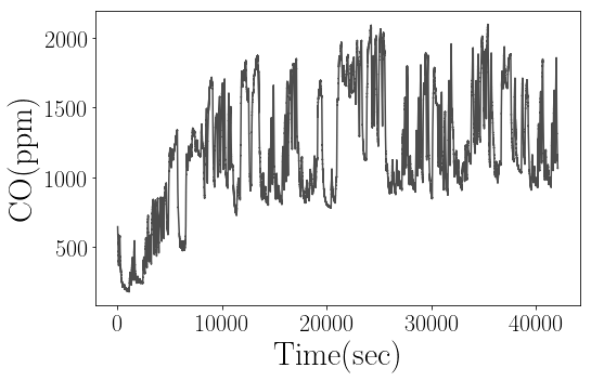
(a) Gas mixture concentrations – Raw

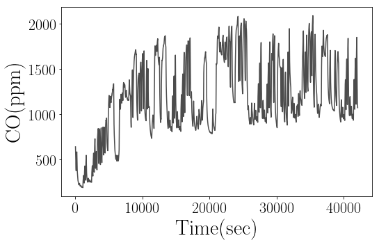
(b) Gas mixture concentrations – Binned with $j=15$

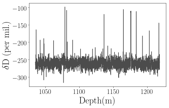
(c) WDC $\delta\text{D}$ – Raw

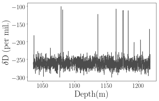
(d) WDC $\delta\text{D}$ – Binned with $j=15$

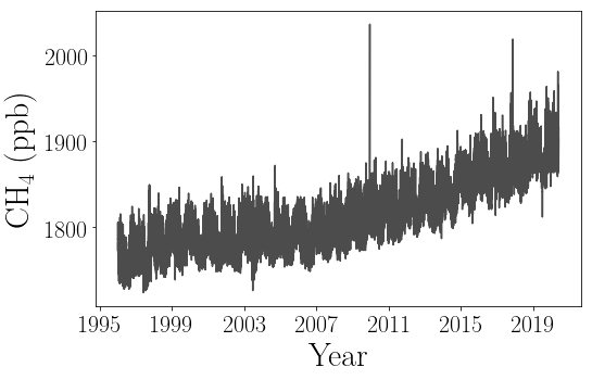
(e) Mauna Loa $CH_{4}$ – Raw

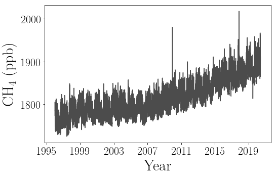
(f) Mauna Loa $CH_{4}$ – Binned with $j=4$

Figure S1: Data sets

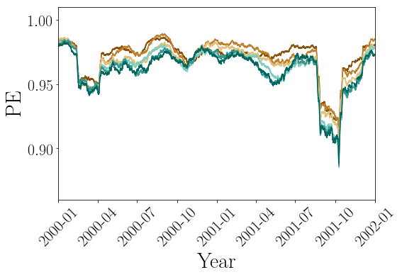
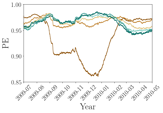
Figure S2: Mauna Loa data: Close-ups showing PE traces of the raw Mauna Loa data.

References

- Bandt and Pompe [2002] C. Bandt and B. Pompe, Permutation entropy: A natural complexity measure for time series, Physical Review Letters 88, 174102 (2002).
- Amigó [2010] J. Amigó, Permutation Complexity in Dynamical Systems: Ordinal Patterns, Permutation Entropy and All That (Springer Science & Business Media, 2010).
- Pennekamp et al. [2019] F. Pennekamp, A. C. Iles, J. Garland, G. Brennan, U. Brose, U. Gaedke, U. Jacob, P. Kratina, B. Matthews, S. Munch, et al., The intrinsic predictability of ecological time series and its potential to guide forecasting, Ecological Monographs 89, e01359 (2019).
- Garland et al. [2014] J. Garland, R. James, and E. Bradley, Model-free quantification of time-series predictability, Physical Review E 90, 052910 (2014).
- Scarpino and Petri [2019] S. V. Scarpino and G. Petri, On the predictability of infectious disease outbreaks, Nature Communications 10, 1 (2019).
- Note [1] The integration step size used to generate the time series also plays a role here; if it is very small, successive points are highly correlated and the will be lower.
- Myers and Khasawneh [2020] A. Myers and F. A. Khasawneh, On the automatic parameter selection for permutation entropy, Chaos 30, 033130 (2020).
- Riedl et al. [2013] M. Riedl, A. Müller, and N. Wessel, Practical considerations of permutation entropy, The European Physical Journal Special Topics 222, 249 (2013).
- Cao et al. [2004] Y. Cao, W.-w. Tung, J. Gao, V. A. Protopopescu, and L. M. Hively, Detecting dynamical changes in time series using the permutation entropy, Physical Review E 70, 046217 (2004).
- Garland et al. [2019] J. Garland, T. R. Jones, M. Neuder, J. W. White, and E. Bradley, An information-theoretic approach to extracting climate signals from deep polar ice cores, Chaos 29, 101105 (2019).
- Garland et al. [2018] J. Garland, T. R. Jones, M. Neuder, V. Morris, J. W. White, and E. Bradley, Anomaly detection in paleoclimate records using permutation entropy, Entropy 20, 931 (2018).
- Amigó et al. [2008] J. M. Amigó, S. Zambrano, and M. A. F. Sanjuán, Combinatorial detection of determinism in noisy time series, Europhysics Letters 83, 60005 (2008).
- Garland et al. [2016] J. Garland, T. R. Jones, E. Bradley, R. G. James, and J. W. White, A first step toward quantifying the climate’s information production over the last 68,000 years, in International Symposium on Intelligent Data Analysis (Springer, 2016) pp. 343–355.
- Myktowicz et al. [2009] T. Myktowicz, A. Diwan, and E. Bradley, Computers are dynamical systems, Chaos 19, 033124 (2009).
- Garland and Bradley [2011] J. Garland and E. Bradley, Predicting computer performance dynamics, in International Symposium on Intelligent Data Analysis (Springer, 2011) pp. 173–184.
- [16] E. Bradley, Damped-driven pendulum dataset, https://bit.ly/2UAuADp.
- Diaconis and Graham [1977] P. Diaconis and R. L. Graham, Spearman’s footrule as a measure of disarray, Journal of the Royal Statistical Society: Series B (Methodological) 39, 262 (1977).
- Kendall [1948] M. G. Kendall, Rank correlation methods., (1948).
- Abdi [2007] H. Abdi, The kendall rank correlation coefficient, Encyclopedia of Measurement and Statistics. Sage, Thousand Oaks, CA , 508 (2007).
- Lorenz [1963] E. N. Lorenz, Deterministic nonperiodic flow, Journal of the Atmospheric Sciences 20, 130 (1963).
- Note [2] For systems with delays, such as those modeled with delay-differential equations, a wider binning window may be required because of the associated temporal propagation of information due to the delay term.
- Mackey and Glass [1977] M. Mackey and L. Glass, Oscillation and chaos in physiological control systems, Science 197, 287 (1977), https://science.sciencemag.org/content/197/4300/287.full.pdf .
- [23] UCI machine learning repository, http://archive.ics.uci.edu/ml.
- Fonollosa et al. [2015] J. Fonollosa, S. Sheik, R. Huerta, and S. Marco, Reservoir computing compensates slow response of chemosensor arrays exposed to fast varying gas concentrations in continuous monitoring, Sensors and Actuators B: Chemical 215, 618 (2015).
- Note [3] We do not have enough data to extend the calculation beyond .
- Dansgaard [1964] W. Dansgaard, Stable isotopes in precipitation, Tellus 16, 436 (1964), https://onlinelibrary.wiley.com/doi/pdf/10.1111/j.2153-3490.1964.tb00181.x .
- Jones et al. [2017a] T. R. Jones, J. W. White, E. J. Steig, B. H. Vaughn, V. Morris, V. Gkinis, B. R. Markle, and S. W. Schoenemann, Improved methodologies for continuous-flow analysis of stable water isotopes in ice cores, Atmospheric Measurement Techniques 10 (2017a).
- [28] T. R. Jones, J. Garland, V. Morris, M. Neuder, E. Bradley, and J. W. C. White, Resampling of deep polar ice cores using information theory, U.S. Antarctic Program (USAP) Data Center. doi: 10.15784/601274.
- Dlugokencky et al. [1995] E. J. Dlugokencky, L. P. Steele, P. M. Lang, and K. A. Masarie, Atmospheric methane at mauna loa and barrow observatories: Presentation and analysis of in situ measurements, Journal of Geophysical Research: Atmospheres 100, 23103 (1995), https://agupubs.onlinelibrary.wiley.com/doi/pdf/10.1029/95JD02460 .
- Note [4] mol per mol dry air.
- McCullough et al. [2016] M. McCullough, K. Sakellariou, T. Stemler, and M. Small, Counting forbidden patterns in irregularly sampled time series. i. the effects of under-sampling, random depletion, and timing jitter, Chaos: An Interdisciplinary Journal of Nonlinear Science 26, 123103 (2016).
- Sakellariou et al. [2016] K. Sakellariou, M. McCullough, T. Stemler, and M. Small, Counting forbidden patterns in irregularly sampled time series. ii. reliability in the presence of highly irregular sampling, Chaos: An Interdisciplinary Journal of Nonlinear Science 26, 123104 (2016).
- Jones et al. [2017b] T. R. Jones, K. M. Cuffey, J. W. C. White, E. J. Steig, C. Buizert, B. R. Markle, J. R. McConnell, and M. Sigl, Water isotope diffusion in the WAIS Divide ice core during the Holocene and last glacial, Journal of Geophysical Research: Earth Surface 122, 290 (2017b).
- Fadlallah et al. [2013] B. Fadlallah, B. Chen, A. Keil, and J. Príncipe, Weighted-permutation entropy: A complexity measure for time series incorporating amplitude information, Physical Review E 87, 022911 (2013).
Acknowledgments
Author Contributions MN, EB, and JG crafted the
research questions. MN, EB, and JG designed the analyses. MN and JG
conducted the analyses. MN, EB, JW, ED, and JG wrote the manuscript and
contributed to discussion and idea development.
Funding: This research was funded by US National
Science Foundation (NSF) grant number 1807478. JG was also partially
supported by an Applied Complexity Fellowship at the Santa Fe
Institute.
Competing Interests The authors declare that they
have no competing financial interests.
Data and materials availability: The gas mixture
data is located in the UCI Machine Learning repository,
archive.ics.uci.edu/ml/machine-learning-databases/00322/.
The ice core data is located in the U.S. Antarctic Program Data
Center,
doi.org/10.15784/601274. The
hourly averages of the Mauna Loa data can be found at
ftp://aftp.cmdl.noaa.gov/data/trace_gases/ch4/in-situ/surface/