On  the  Beamforming  Design  of  Millimeter  Wave  UAV  Networks:  Power  vs.  Capacity  Trade-Offs

Abstract

The millimeter wave (mmWave) technology enables unmanned aerial vehicles (UAVs) to offer broadband high-speed wireless connectivity in fifth generation (5G) and beyond (6G) networks. However, the limited footprint of a single UAV implementing analog beamforming (ABF) requires multiple aerial stations to operate in swarms to provide ubiquitous network coverage, thereby posing serious constraints in terms of battery power consumption and swarm management. A possible remedy is to investigate the concept of hybrid beamforming (HBF) transceivers, which use a combination of analog beamformers as a solution to achieve higher flexibility in the beamforming design. This approach permits multiple ground users to be served simultaneously by the same UAV station, despite involving higher energy consumption in the radio frequency (RF) domain than its ABF counterpart. This paper presents a tractable stochastic analysis to characterize the downlink ergodic capacity and power consumption of UAV mmWave networks in an urban scenario, focusing on the trade-off between ABF and HBF architectures. A multi-beam coverage model is derived as a function of several UAV-specific parameters, including the number of UAVs, the deployment altitude, the antenna configuration, and the beamforming design. Our results, validated by simulation, show that, while ABF achieves better ergodic capacity at high altitudes, an HBF configuration with multiple beams, despite the use of more power-hungry RF blocks, consumes less power all the time with limited capacity degradation.

I Introucion

While Long Term Evolution (LTE) networks are already successfully penetrating new markets, and with 5th generation (5G) deployments ready for global commercial roll-out, the more stringent traffic requirements of future wireless applications (which will reach 1 zettabyte/month in 2028 [1]) are driving the research community to discuss new services and enabling technologies towards 6th generation (6G) systems [2]. Notably, not only will current terrestrial infrastructures facing greater capacity demands not guarantee the required Quality of Service (QoS), but they will also show vulnerability in emergency situations (such as disaster relief/recovery), a research challenge that communication standards have, so far, relegated to the very bottom, if not entirely ignored [3].

To address this issue, 6G research is focusing on the development of non-terrestrial networks (NTNs) where air/spaceborne stations like Unmanned Aerial Vehicles (UAVs), High Altitude Platforms (HAPs), and satellites assist terrestrial infrastructures in promoting flexible and cost-effective global connectivity [4, 5]. Thanks to their high mobility, versatility, and low cost, UAVs, in particular, play a key role in providing network service recovery in devastated region, enhancing public safety, and handling emergency situations[6, 7, 8, 9].

In combination with the millimeter wave (mmWave) technology, whose huge available bandwidth can offer multi-Gbps data rates [10], UAVs may also serve as aerial relays and base stations to support wireless services in high-traffic scenarios, e.g., to assist backhaul operations when terrestrial towers are overloaded [11], and/or to relay large amounts of sensor data in hot-spot areas from multiple ground users (GUs) [12]. However, mmWave communications may incur severe path loss and sensitivity to blockage, especially considering the very long transmission distances involved [13], which may result in QoS degradation. In these regards, massive Multiple Input Multiple Output (MIMO) techniques have been introduced to improve reliability and spectral efficiency through beamforming [10]. The short wavelength of mmWave signals, indeed, permits multiple antenna elements to be placed into a small UAV to form a concentrated beam pattern towards a specific direction, thus providing array gains and reduced co-channel interference [14].

In the UAV context, the limited energy and payload resources of aerial systems make it difficult, if not impossible, to realize full-blown digital beamforming (DBF) which, while potentially enabling the transceiver to direct beams at infinitely many directions, requires a dedicated Radio Frequency (RF) chain for each antenna element [15]. An analog beamforming (ABF) structure, in turn, adopts the simplest electronic components and requires a single RF chain, thus theoretically representing the most desirable option to achieve low power consumption [16]. The limited flexibility of ABF, however, means that UAVs can only beamform in one direction at a time, and forces multiple aerial stations to be deployed in formation to provide ubiquitous network coverage to GUs: this may incur significant energy consumption for propulsion and hovering as the swarm grows in size, thereby posing severe power management constraints. In this context, the research community is leaning towards the development of hybrid beamforming (HBF), which realizes a simple transceiver design by combining RF analog beamformers and low-dimensional baseband digital beamformers [17, 18]. In particular, HBF enables simultaneous transmission of multiple data streams from the same UAV station, and makes it possible to reduce the UAV swarm size and its relative cost compared to ABF. Despite these premises, however, few contributions have been devoted to the evaluation of the performance of HBF in a UAV scenario, which in turn represents a timely research issue.

Following this rationale, in this paper we provide the first analytical model to jointly evaluate and compare the ergodic capacity and power consumption of ABF and HBF architectures for UAV networks. The main novelty of our work can be summarized as follows:

• We provide a mathematical and tractable expression for the ergodic capacity of UAVs operating at mmWave frequencies based on stochastic geometry. Compared to previous analyses, which employ a specific beamforming design (e.g., [19, 20]), in this work we compare the performance of the ABF and HBF configurations as a function of the UAV deployment altitude, the antenna architecture, and the density of GUs. For these two types of beamforming strategies, two approximate antenna patterns (based on a flat-top model that accounts for both direct and tilted beams) are proposed to achieve a good balance between accuracy and analytical tractability.

• We provide an analytical expression for the power consumed by UAVs when establishing ABF and HBF transmissions. Our model accounts for both the hovering power, which is required to maintain the UAV aloft and enable its mobility, as well as the power consumed by each MIMO electronic component for communication. We discuss the impact of the number of RF chains and antenna elements on the beamforming design, the UAV deployment altitude, and the resolution of the Digital to Analog Converter (DAC), i.e., the most power-hungry hardware block in the transmitter.

• Based on the above-mentioned relations, while existing analyses tend to separate coverage- (e.g., [21, 22]) and power-related (e.g., [23, 24]) performance, we provide a new paradigm to jointly evaluate the coverage vs. power consumption trade-off for mmWave-assisted UAV networks. Our theoretical model is validated via realistic Monte Carlo simulations, so as to include many more details than would be possible via analytical evaluations while accounting for realistic channel implementations. Despite the common belief that HBF suffers from higher energy consumption than ABF, we demonstrate that HBF with two or three simultaneous beams always outperforms an ABF strategy at low altitude in terms of both power efficiency and capacity, especially when increasing the antenna array size. Conversely, ABF exhibits better capacity at higher altitudes, even though HBF’s degradation is limited. Specifically, we demonstrate that the user’s density qualifies as the most crucial factor in the capacity performance.

• We provide guidelines on the optimal beamforming strategy to adopt to minimize power consumption while not sacrificing spectral efficiency. We show that, with the increasing UAV altitude, the system capacity has a peak value that depends on the density of GUs and the antenna array size, above which the system would consume more power.

The remainder of this paper is organized as follows. Related works on UAV mmWave networks are discussed in Sec. II. Sec. III describes our system model, including the scenario, channel, antenna, and power consumption models for both ABF and HBF architectures. In Sec. V and Sec. IV we derive the expressions of the power consumption and ergodic capacity for ABF and HBF, respectively. Sec. VI reports our system parameters, validates our theoretical framework through simulations, and presents our main findings and results. Finally, conclusions and suggestions for future work are provided in Sec. VII.

II Related Work

UAV-assisted mmWave networks have been extensively studied in the literature. Xiao et al., for example, reviewed the main opportunities and challenges associated with high-frequency UAV operations [25], Xia et al. discussed applications of mmWaves in UAV-enabled public safety scenarios [26], while Zhao et al. evaluated the performance of integrated flight control and channel tracking for mmWave aerial links [27]. More recent works are now focusing on analyzing the coverage and data rate performance, beamforming design, and power consumption of the network, as discussed in the following paragraphs.

Coverage/rate performance

Stochastic geometry has emerged as a tractable approach to study the coverage performance of wireless systems. In the UAV context, papers [20, 28, 19, 29] derived lower and upper bounds for the coverage probability and the area spectral efficiency of UAV networks, while in our related work [22] we identified the trade-offs to be considered to maximize the coverage performance as a function of the drone density, height, and antenna patterns. More recently, the article in [30] investigated the coverage performance of UAV mmWave networks when UAVs are assumed to be distributed according to a homogeneous Poisson Point Process (PPP) and users are modeled as a Poisson Cluster Process (PCP, e.g., Thomas cluster processes or Matern cluster processes). For the proposed system, simulation results indicated that there exists an optimal altitude that maximizes the coverage probability, and that the effect of the thermal noise and non-line of sight transmissions can be omitted. Related work [31] adopted a similar model for the deployment of UAVs and GUs, and formulated a mathematical expression for the average uplink throughput to identify the optimal time division multiplexing between the downlink and uplink phases. Similarly, the authors in [32] compared the performance of LTE and mmWave networks for serving flying UAVs. The results demonstrated that a significant improvement of the UAV coverage probability is possible using mmWaves, even though inter-cell interference remains a key performance challenge at high altitudes. Another approach was considered in [33], where the authors provided a closed-form expression for the maximum achievable rate for a full-duplex UAV scenario, and proposed an alternating interference suppression algorithm to jointly design the beamforming vectors and the power control variables. Moreover, Xiao et al. [34] formulated a non-convex problem to maximize the achievable data rate, subject to user requirements, UAV positions, and beamforming vector constraints.

Energy consumption

Despite demonstrating promising coverage performance, there are still several challenges associated to UAV-enabled networks, ranging from energy limitations to optimal 3D deployment. In the literature, Mozaffari et al. [35] determined the optimal UAV altitude to minimize the transmitted power, while the authors in [23] proposed a coverage-aware path planning method to reduce energy consumption while satisfying data rate and resolution constraints. Several other related works, e.g., [36, 37], have also analyzed the energy trade-offs associated with UAV propulsion, which involves significantly higher power consumption compared to conventional (static) terrestrial stations.

In this perspective, the utilization of the mmWave technology for drone-assisted communications also resulted in higher power utilization for electronic components like DACs, phase shifters and combiners, and power amplifiers, which are required to process a large number of antenna outputs and very wide bandwidths. In a recent work [38], the authors explored how DAC resolution and bandwidth affect the total power consumption, while [39] studied the energy performance of mmWave systems as a function of different pre-coding and post-coding beamforming structures. However, most literature is referred to a cellular-type scenario, while only a few papers have investigated energy efficiency for UAV networks [37, 24], which therefore represents a timely topic for further research.

Beamforming design

Sharp beamforming is necessary to support UAV communications at mmWaves. Along these lines, Miao et al. [40] first formalized a robust beamforming optimization problem to maximize network coverage under the constraint of strong interference. Similarly, the authors in [41] explored how to design the optimal beam according to the drone flying range, while paper [42] presented an innovative position-based lightweight beamforming technology to enhance broadcasting communications through UAVs. More recently, Li et al. [43] proposed to jointly optimize UAV trajectory and beamforming design through reconfigurable intelligent surfaces, thus improving propagation environment and enhancing communication quality. While full DBF cannot be adopted on UAVs because of the high cost and energy consumption, HBF solutions have been proposed to improve communication performance while minimizing power utilization, e.g., [44]. A similar approach was followed in [45], even though the literature does not carefully demonstrate whether (and in which form) HBF outperforms a pure ABF configuration from both a coverage and an energy efficiency point of view.

Our work differs from the prior art in that we compare different beamforming architectures, optimizing both power consumption and coverage performance together. Moreover, our power model does not only consider hovering operations, but it also characterizes the energy impact for communication in the UAV context.

III System Model

In this section we present our system scenario (Sec. III-A), channel (Sec. III-B), antenna (Sec. III-C), and power (Sec. III-D) models that are considered in our study.

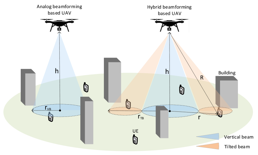
Fig. 1: UAV-assisted system model. UAVs can form vertical and/or tilted beams, depending on the beamforming architecture (ABF or HBF, respectively) they adopt.

III-A Scenario Description

As shown in Fig. 1, we consider a UAV-assisted urban scenario in which mmWave-enabled swarms of drones acting as aerial base stations are deployed at altitude $h$ to provide communication services on the ground. Furthermore, we assume that GUs are placed across a circular Area of Interest (AoI) to form a two-dimensional (2D) homogeneous PPP $\Phi_{u}$ with density $\lambda_{u}$. We assume that both UAVs and GUs communicate through directional beams whose width, shape, and structure depend on the beamforming strategy they adopt, as we will specify in Sec. III-C. We then call $r$ the 2D distance between the projection of the UAV on the user plane and a generic GU in the AoI, and $R=\sqrt{r^{2}+h^{2}}$ the distance between the reference UAV and the GU.

III-B Channel Model

III-B1 Line-of-sight probability

In the urban scenario, air-to-ground communication links may be blocked by environmental structures such as buildings or vegetation. Therefore, it is essential to distinguish between line of sight (LOS) and non-line of sight (NLOS) propagation (denoted respectively with subscripts $L$ and $N$ throughout the paper). The International Telecommunication Union (ITU) presents a precise expression for the LOS probability [46], which is estimated by ray-tracing techniques using data from building and terrain databases. For the purpose of mathematical tractability, in this paper we adopt a simplified equation, proposed in prior work [47] and universally adopted in the literature, in which the LOS probability $p_{L}(r)$ is modeled, as a function of the GU-UAV distance $R=\sqrt{r^{2}+h^{2}}$, as a modified Sigmoid function (S-curve), i.e.,

$$p_{L}(r)=\frac{1}{1+p\>\mathrm{exp}\left[-q\left(\arctan\Big{(}\frac{h}{\sqrt{r^{2}+h^{2}}}\Big{)}\frac{180}{\pi}-p\right)\right]},$$ (1)

where $\arctan({h}/\sqrt{r^{2}+h^{2}})$ is the elevation angle of the UAV, and $p$ and $q$ are the S-curve parameters which depend on the environment (suburban, urban, dense urban, high-rise urban). Consequently, the NLOS probability is given by $p_{N}(r)=1-p_{L}(r)$. By the thinning theorem of PPPs, we can thus distinguish two independent PPPs for the LOS and NLOS GUs, i.e., $\Phi_{u,L}\subseteq\Phi_{u}$ and $\Phi_{u,N}\subseteq\Phi_{u}$, respectively, of intensity measures $\lambda_{u,L}=p_{L}(r)\lambda_{u}$ and $\lambda_{u,N}=p_{N}(r)\lambda_{u}$.

III-B2 Path gain

We consider the widely adopted power-law model for the path gain [48], i.e.,

$$\ell_{i}(r)=\eta_{i}R^{-\kappa_{i}}=\eta_{i}(\sqrt{r^{2}+h^{2}})^{-\kappa_{i}},\quad i\in\{L,\,N\}.$$ (2)

In Eq. (2), $\kappa_{i}$ is the path loss exponent and $\eta_{i}$ is the path loss gain at unit distance. Due to the signal propagating in NLOS suffering from shadowing and reflection effects from obstacles, it holds $\eta_{\mathrm{L}}>\eta_{\mathrm{N}}$ and $\kappa_{\mathrm{L}}<\kappa_{\mathrm{N}}$.

III-B3 Small-scale fading

Even though measurements conducted in the mmWave environment show a relatively small impact of fading on propagation [49], the effect of small-scale fading due to reflectivity and scattering from common objects may not be negligible in the UAV scenario, especially when directional beamforming is applied [50]. In this paper, small-scale fading is modeled as a Nakagami-m random variable $\gamma_{i}$ of parameters $m_{i}$ and $\Omega_{i}$, $i\in\{L,N\}$, which is typically adopted to represent both LOS and NLOS air-to-ground channels, whose Cumulative Distribution Function (CDF) is given by [51]:

$$F(x;m_{i},\Omega_{i})=\mathbb{P}[\gamma_{i}(m_{i},\Omega_{i})\leq x]=$$

$$P\left(m_{i},\frac{m_{i}}{\Omega_{i}}x^{2}\right)=\frac{2m_{i}^{m_{i}}x^{2m_{i}-1}}{\Omega_{i}^{m_{i}}\Gamma(m_{i})}\ \mathrm{exp}\left(\frac{-m_{i}x^{2}}{\Omega_{i}}\right).$$ (3)

In Eq. (3), $\Omega_{i}$ is the spread factor, $m_{i}$ is the shape factor, and $\Gamma(\cdot)$ is the Gamma function.

III-C Antenna Model

In this paper we assume that UAVs are equipped with Uniform Planar Arrays (UPAs) of $N_{T}=N_{x}\times N_{y}$ antenna elements, separated in the horizontal and vertical dimension by $d_{x}$ and $d_{y}$, respectively, providing gain by beamforming. For simplicity, we assume square UPAs, i.e., $N_{x}=N_{y}$, and $d_{x}=d_{y}=d$. Further, we consider a flat-top model to characterize the pattern of the directional beamforming. UAVs implementing ABF shape the beam through a single RF chain for all the antenna elements, and can form a single vertical beam (VB) perpendicular to the ground (the blue beams in Fig. 1). In this case, the processing is performed in the analog domain, thus transmitting/receiving in only one direction at a time [13]. UAVs implementing HBF, in turn, use $N_{RF}$ RF chains (with $N_{RF}\leq N_{T}$) that allow to produce, besides the analog VB, $N_{D}-1$ additional parallel tilted beams (TBs), with $N_{D}\leq N_{RF}$, towards the ground (the orange beams in Fig. 1). This permits the transceiver to transmit/receive in $N_{D}$ directions simultaneously, thus improving flexibility compared to ABF, at the cost of a higher power consumption.

Lemma 1

Based on the above assumptions, the main lobe directivity gain $G$ for a UPA produced by beamforming can be expressed as

$$G=N_{x}\cdot N_{y}.$$ (4)

Proof: For UPAs, the array factors (AFs) of the arrays in the x- and y-directions, for any pair of vertical and horizontal angles $(\theta,\phi)$, $\forall\theta\in[0,\pi],\>\forall\phi\in[-\pi,\pi]$, can be written as

$$\mathrm{AF}(\theta,\phi)= \sum_{n_{y}=1}^{N_{y}}\left[\sum_{n_{x}=1}^{N_{x}}e^{j(2\pi/\lambda)[(n_{x}-1)d_{x}\sin\theta\cos\phi]}\right]$$

$$\cdot e^{j(2\pi/\lambda)[(n_{y}-1)d_{y}\sin\theta\sin\phi]},$$ (5)

where $\lambda$ is the wavelength. Inspired by [52] and [53], which derived the instantaneous directivity gain of Uniform Linear Arrays (ULAs) transmitters, the array gain of UPAs can be recast as

$$G_{t}(\Delta\theta,\Delta\phi) =N_{x}N_{y}\left[\mathrm{AF}(\Delta\theta,\Delta\phi)\right]^{2}$$

$$\overset{(a)}{=}\left[\frac{\sin^{2}(\pi N_{x}\psi_{x})}{N_{x}\sin^{2}(\pi\psi_{x})}\right]\left[\frac{\sin^{2}(\pi N_{y}\psi_{y})}{N_{y}\sin^{2}(\pi\psi_{y})}\right],$$ (6)

where

$$\psi_{x}=\frac{d_{x}}{\lambda}\sin(\Delta\theta)\cos(\Delta\phi),$$

$$\psi_{y}=\frac{d_{y}}{\lambda}\sin(\Delta\theta)\cos(\Delta\phi),$$ (7)

and $(a)$ follows from [54]. Assuming that the optimal beamforming vector is used, i.e., $\Delta\theta=\Delta\phi=0$, the antenna gain is then given by

$$G=G_{t}(0,0)=N_{x}\cdot N_{y}.$$ (8)

$\blacksquare$

III-D Power Model

In our model, we consider the power for hovering, which maintains the UAV aloft and permits its mobility, and for communicating to the GUs in both ABF and HBF configurations.

III-D1 Hovering Power

The power consumption model of multi-rotor UAVs include three components [55]: (i) induced power ($P_{\mathcal{I}}$), which produces thrust by propelling air downwards, (ii) profile power ($P_{\mathcal{P}}$), which overcomes the rotational drag of rotating propellers, and (iii) parasite power ($P_{par}$), which resists body drag between the UAV and the wind. These components are expressed as

$$P_{\mathcal{I}}(T,V_{vert})=k_{1}T\left[\tfrac{V_{vert}}{2}+\sqrt{(\tfrac{V_{vert}}{2})^{2}+\tfrac{T}{k_{2}^{2}}}\right],$$ (9)

$$P_{\mathcal{P}}(T,V_{air})=c_{2}\sqrt{T^{3}}+c_{3}(V_{air}\cos\alpha_{a})^{2}\sqrt{T},$$ (10)

$$P_{par}(V_{air})=c_{4}V_{air}^{3},$$ (11)

$$T=\sqrt{[mg-(c_{5}(V_{air}\cos\alpha)^{2}+c_{6}T)]^{2}+(c_{4}V_{air}^{2})^{2}},$$ (12)

where $T$, $mg$, and $V_{vert}$ are the UAV thrust, gravity, and vertical speed, $V_{air}$ is the horizontal airspeed, and $\alpha_{a}$ is the angle of attack. $k_{1}$, $k_{2}$, $c_{2}$, $c_{3}$, $c_{4}$ and $c_{5}$ are related constant parameters. When the vertical speed and the horizontal airspeed are equal to zero (e.g., when considering UAVs hovering at fixed locations, as assumed in this study), the hovering power consumption can be expressed as

$$P_{hover} =P_{\mathcal{I}}(T,0)+P_{\mathcal{P}}(T,0)+P_{par}(0)$$

$$=(c_{1}+c_{2})(mg)^{3/2},$$ (13)

where $c_{1}=k_{1}/k_{2}$. The hovering power consumption determines the maximum UAV endurance, range, and flight speed, which, based on Eq. (13), mainly depends on the UAV gravity.

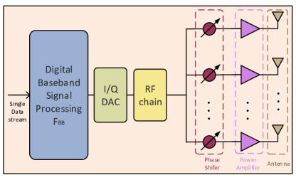
Fig. 2: ABF architecture with single RF chain.

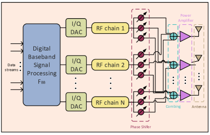
Fig. 3: HBF architecture with multiple RF chains.

III-D2 Communication Power

The ABF and HBF architectures are shown in Figs. 3 and 3, respectively. The total static power consumption of each scheme required for communication towards the ground can be evaluated by the following expressions [56]:

$$P_{\rm ABF}=P_{PA}+2P_{DAC}+P_{RF}+P_{SP}+N_{T}(P_{PS}),$$ (14)

$$P_{\rm HBF}=P_{PA}+N_{RF}\left(2P_{DAC}+P_{RF}+P_{SP}\right)$$

$$\qquad\quad\>+N_{T}(N_{RF}P_{PS}+P_{C}),$$ (15)

where $N_{T}$ is the total number of antenna elements in the UAV’s array, $N_{RF}$ is the number of RF chains, and $P_{PA}$, $P_{PS}$, $P_{SP}$, $P_{C}$ represent the power consumptions of the power amplifier, phase shifter, splitter, and combiner, respectively. In Eqs. (14) and (15), $P_{RF}$ and $P_{DAC}$ identify the power consumption of the RF chain and DAC, respectively. We consider an RF phase shifting approach, which modifies the phase on the RF path directly. Moreover, we deploy DACs with a binary-weighted current-steering topology which does not involve buffering, thus allowing high-speed conversions [57]. Hence, power consumption can be evaluated respectively as

$$P_{RF}=P_{M}+P_{LO}+P_{LPF}+P_{H}+P_{BBamp},$$ (16)

$$P_{DAC}=1.5\times 10^{-5}\cdot 2^{b_{DAC}}+9\times 10^{-12}\cdot b_{DAC}\cdot F_{S},$$ (17)

where $P_{M}$, $P_{LO}$, $P_{LPF}$, $P_{H}$, $P_{BBamp}$ are the power consumption of mixer, local oscillator, low pass filer, $90$-degree hybrid coupler with buffer, and base-band amplifier, while $F_{S}$ and $b_{DAC}$ are the DAC sampling frequency and resolution, respectively.

Overall, considering both UAV hovering and communication modules, the total power consumption for a UAV-assisted mmWave transmitter can be expressed by

$$P_{\rm tot}^{\rm ABF}=P_{ABF}+P_{hover},$$ (18)

$$P_{\rm tot}^{\rm HBF}=P_{HBF}+P_{hover}.$$ (19)

IV Power Consumption Analysis

In this section, we first calculate the main lobe half-power beamwidth (HPBW) of the VB and TBs (Sec. IV-A), then we derive an analytical expression for the power consumed by UAVs implementing ABF or HBF to provide connectivity to a certain AoI of size $S_{\rm tot}$ (Sec. IV-B).

IV-A Coverage Model

The main lobe HPBW for a UPA is given by [54]

$$\Theta_{P}(\theta,\phi)=\sqrt{\frac{1}{\cos^{2}\theta[\Theta_{L_{x}}^{-2}\cos^{2}\phi+\Theta_{L_{y}}^{-2}\sin^{2}\phi]}},$$ (20)

where $\theta$ and $\phi$ represent the antenna elevation and azimuth angles, respectively. In Eq. (20), $\Theta_{L_{x}}$ ($\Theta_{L_{y}}$) is the HPBW for a ULA of $N_{x}$ ($N_{y}$) elements along the x-axis (y-axis), i.e.,

$$\Theta_{L_{i}}=\pi-2\cos^{-1}\left(\tfrac{1.391}{\pi\rho N_{T}}\right),\quad i\in\{x,\,y\},$$ (21)

where $\rho=d/\lambda$, $d$ is the antenna separation, $\lambda$ is wavelength, and $N_{T}=N_{x}\times N_{y}$ is the total number of antenna elements. For the VB, which is perpendicular to the ground (i.e., ${\theta=0}$), the HPBW can be calculated directly as

$$\Theta_{P}^{\rm VB}=\Theta_{P}(0,\phi).$$ (22)

(a) HPBW of vertical beam $\Theta_{P}^{\rm VB}$.

(b) HBPW of tilted beams $\Theta_{P}^{\rm TB}$.

Fig. 4: Half-power beamwidth for different values of the antenna array size and antenna element separation distance.

As such, we define $r_{\rm VB}=h\tan(\Theta_{P}^{\rm VB}/2)$ the radius of the coverage area shaped by the VB, as depicted in Fig. 1. For the TBs, which are adjacent to the VB, the HPBW is

$$\Theta_{P}^{\rm TB}=\Theta_{P}\left((\Theta_{P}^{\rm VB}+\Theta_{P}^{\rm TB})/2,\phi\right).$$ (23)

In this case, we call $r_{\rm TB}=h\tan(\Theta_{P}^{\rm VB}/2+\Theta_{P}^{\rm TB})$ the distance between the projection of the UAV on the ground plane and the edge of the footprint shaped by the TB, as depicted in Fig. 1. In Fig. 4, we illustrate how the HPBW scales as a function of $\rho$ and $N_{T}$. The results show that, while TBs exhibit a larger HPBW, especially when $\rho$ is small, the footprint of both VB and TBs is inversely proportional to the antenna size and grows with the antenna separation distance.

Theorem 1

According to the coverage model introduced above, the (circular) coverage area of a VB and the (oval) coverage area of a single TB are derived respectively as

$$S_{\rm VB}=\pi r_{\rm VB}^{2},$$ (24)

$$S_{\rm TB}=\pi ab,$$ (25)

where parameters $a$ and $b$, which represent the two semi-axes of an ellipse, are given by

$$a=\tfrac{1}{2}\cdot h[\tan(\Theta_{H}^{\rm VB}+\Theta_{P}^{\rm TB})-\tan(\Theta_{H}^{\rm VB})],$$ (26)

$$b= \Big{\{}(\sin\Theta_{H}^{\rm TB})^{2}-\Big{[}\cos\Theta_{H}^{\rm VB}\cdot\tan(\pi/2-\Theta_{H}^{\rm VB}-\Theta_{H}^{\rm TB})-$$

$$-\arctan\left(\tfrac{h}{a+h\tan\Theta_{H}^{\rm VB}}\right)\Big{]}^{2}\Big{\}}^{1/2}/$$

$$\Big{[}{\cos(\Theta_{H}^{\rm VB}+\Theta_{P}^{\rm TB})\cdot\cos(\Theta_{H}^{\rm TB}/2)\cdot\sec(\Theta_{H}^{\rm VB}+\Theta_{H}^{\rm TB})}\Big{]}\cdot$$

$$\frac{\csc\left(\arctan\left(\tfrac{h}{a+h\tan\Theta_{H}^{\rm VB}}\right)\right)}{\sec\left(\pi/2-\Theta_{H}^{\rm VB}-\Theta_{H}^{\rm TB}-\arctan\left(\tfrac{h}{a+h\tan\Theta_{H}^{\rm VB}}\right)\right)},$$ (27)

and $\Theta_{H}^{i}$ is the half of $\Theta_{P}^{i}$, $i\in\{\text{VB,TB}\}$.

Proof: It is obvious that the VB covers a circular area of radius $r_{\rm VB}=h\tan(\Theta_{H}^{\rm VB})$. For the VBs, it is common knowledge that the cross section of a cone and plane is an ellipse, which proves the assumption that TBs cover an oval area. The length of the two semi-axes of the ellipse can be derived by applying the well-known properties of similar triangles, and the details are omitted here. $\blacksquare$

Therefore, the coverage area of an ABF UAV, shaping one single VB, and that of an HBF UAV, forming $N_{D}$ parallel beams, can be expressed as

$$S_{\rm ABF}=S_{\rm VB},$$ (28)

$$S_{\rm HBF}=S_{\rm VB}+(N_{D}-1)S_{\rm TB}.$$ (29)

IV-B Power Consumption

Finally, we can evaluate the power consumed by the UAVs to provide coverage service to an AoI of size $S_{\rm tot}$. Let $N_{\rm ABF}=\lceil{S_{\rm tot}}/{S_{\rm ABF}}\rceil$ and $N_{\rm HBF}=\lceil{S_{\rm tot}}/{S_{\rm HBF}}\rceil$ be the number of UAVs required to cover the AoI in case ABF or HBF is implemented, respectively. Overall, the total power consumption (which is due to both hovering and communication) for the ABF and HBF configurations is given based on Eqs. (18) and (19) by

$$P_{C}^{\rm ABF}=N_{\rm ABF}\cdot P_{\rm tot}^{\rm ABF}=N_{\rm ABF}\cdot(P_{hover}+P_{\rm ABF}),$$ (30)

$$P_{C}^{\rm HBF}=N_{\rm HBF}\cdot P_{\rm tot}^{\rm HBF}=N_{\rm HBF}\cdot(P_{hover}+P_{\rm HBF}).$$ (31)

V Stochastic Ergodic Capacity Analysis

In this section, we evaluate the stochastic ergodic capacity of a mmWave UAV network implementing ABF or HBF. Specifically, in Sec. V-A we present the association rule for the GUs and provide a probabilistic expression for the UAV-GU serving distance, while in Secs. V-B and V-C we derive the ergodic capacity experienced in the VB or TBs and when configuring ABF or HBF, respectively.

V-A Association Probabilities

In order to facilitate the analysis, we evaluate the association probabilities between a reference UAV and GUs from a 2D perspective. Specifically, we make the assumption that UAVs form their beam(s) towards and communicate with the closest available GUs within their respective coverage regions. Indeed, let $r_{n}$ be the distance between the projection of the reference UAV on the user plane and the $n$-th closest user on the ground, which means that there are $(n-1)$ GUs at distance smaller than $r_{n}$. Since the process $\Phi_{u}$ for the GUs’ distribution is a 2D homogeneous PPP with intensity measure $\lambda_{u}$, we can derive the CDF $F_{r_{n}}(r)$ of $r_{n}$ as [58]

$$F_{r_{n}}(r) =1-\mathbb{P}[r_{n}>r]$$

$$=1-\mathbb{P}[(n-1)\>\textrm{GUs closer than}\>r]$$

$$=1-e^{-\lambda_{u}\pi r^{2}}\sum_{k=1}^{n-1}\frac{(\lambda_{u}\pi r^{2})^{k}}{(k-1)!}.$$ (32)

Consequently, the probability density function (pdf) of $r_{n}$ can be derived as

$$f_{r_{n}}(r) =\frac{\mathrm{d}F_{r_{n}}(r)}{\mathrm{d}r}=r^{2n-1}(\lambda_{u}\pi)^{n}\frac{2}{(n-1)!}e^{-\lambda_{u}\pi r^{2}}.$$ (33)

$$\tau^{\rm VB}=B\int_{0}^{r_{\rm VB}}\int_{0}^{\infty}\int_{0}^{\infty}\frac{\left(l^{m_{L}-1}+\sum_{j=2}^{m_{L}}\frac{\Gamma(m_{L})}{(m_{L}-j)!}l^{m_{L}-j}\right)e^{-\Delta_{L}}}{(m_{L}-1)!}f_{r_{1}}^{\rm VB}(r)p_{\gamma}(\gamma_{N})\mathrm{d}\gamma_{N}\mathrm{d}t\mathrm{d}r$$ (37)

$$\tau^{\rm TB}=B\int_{0}^{r_{\rm TB}}\int_{0}^{\infty}\int_{0}^{\infty}\frac{\left(l^{m_{L}-1}+\sum_{j=2}^{m_{L}}\frac{\Gamma(m_{L})}{(m_{L}-j)!}l^{m_{L}-j}\right)e^{-\Delta_{L}}}{(m_{L}-1)!}f_{r_{\tilde{n}}}^{\rm TB}(r)p_{\gamma}(\gamma_{N})\mathrm{d}\gamma_{N}\mathrm{d}t\mathrm{d}r$$ (39)

 

In case a single (vertical) beam is formed, i.e., ABF or HBF with $N_{D}=1$, the reference UAV steers the VB towards the closest GU. We can then evaluate the pdf of the 2D distance between the UAV and the closest GU, i.e., $r_{1}$, from Eq. (33) as

$$f_{r_{1}}^{\rm VB}(r)=e^{-\lambda_{u}\pi r^{2}}2\pi\lambda_{u}r.$$ (34)

Since GUs’ distribution is PPP with density $\lambda_{u}$, the average number of users within VB’s footprint is equal to $\lambda_{u}S_{\rm VB}=\pi\lambda_{u}r_{\rm VB}^{2}$, where $r_{\rm VB}=h\tan(\Theta_{P}^{\rm VB}/2)$ is the radius of the coverage area described by the VB, as discussed in Sec. IV-A.

In case tilted beams are also available, i.e., HBF with $2\leq N_{D}\leq N_{RF}$, the reference UAV forms a TB towards the $\tilde{n}$-th closest GU, with $\widetilde{n}=\mathrm{floor}(\lambda_{u}\pi r_{\rm VB}^{2})+1$ corresponding to the first GU outside VB’s coverage. Based on the above definition, we can evaluate the pdf of the 2D distance between the UAV and the $\tilde{n}$-th closest GU, i.e., $r_{\tilde{n}}$, from Eq. (33) as

$$f_{r_{\tilde{n}}}^{\rm TB}(r)=r^{2{\tilde{n}}-1}(\lambda_{u}\pi)^{{\tilde{n}}}\frac{2}{({\tilde{n}}-1)!}e^{-\lambda_{u}\pi r^{2}}.$$ (35)

V-B Ergodic Capacity of Vertical and Tilted Beams

In this subsection we provide an analytical closed-form expression for the ergodic capacity $\tau^{\rm VB}$ and $\tau^{\rm TB}$ for a target GU within a VB or TB, respectively. The ergodic capacity is a function of the Signal to Noise Ratio (SNR) experienced by the GU attached to a reference UAV at distance $R=\sqrt{r^{2}+h^{2}}$ which, due to the presence of LOS and NLOS conditions for the channel, can be expressed as a function of $r$ as:

$$\text{SNR}(r)=\frac{P_{t}G\left[\gamma_{L}p_{L}(r)\ell_{L}(r)+\gamma_{N}p_{N}(r)\ell_{N}(r)\right]}{N_{D}\cdot\mathrm{NF}\cdot\sigma^{2}}.$$ (36)

In Eq. (36), $P_{t}$ is the total transmitter power, $G$ is the beamforming gain, $\gamma_{i}$, $p_{i}(r)$, and $\ell_{i}(r)$, $i\in\{L,N\}$, represent, as introduced in Sec. III-B, the small-scale fading, LOS probability, and path gain, respectively, $\mathrm{NF}$ is the noise figure, and $\sigma^{2}$ is the power of the thermal noise. Furthermore, $1\leq N_{D}\leq N_{RF}$ is the number of beams produced by the UAV simultaneously (where, of course, $N_{D}=1$ for ABF).

Theorem 2

The ergodic capacity for a target GU located within a VB can be written as in Eq. (37), where $\Delta_{L}=m_{L}/\Omega_{L}\cdot\beta(t,\gamma_{N})$, $B$ is the system bandwidth, $p_{\gamma}(\gamma_{N})$ is the probability distribution of the small-scale fading for NLOS propagation, and

$$\beta(t,\gamma_{N})=\frac{(e^{t\ln 2}-1)N_{D}\mathrm{NF}\sigma^{2}-P_{t}G\gamma_{N}p_{N}(r)\ell_{N}(r)}{P_{t}Gp_{L}(r)\ell_{L}(r)}.$$ (38)

Proof: The proof is given in Appendix A. $\blacksquare$

Theorem 3

The ergodic capacity for a target GU located within a TB can be written as in Eq. (39), where $r_{\rm TB}$ is the distance between the projection of the UAV on the ground plane and the farthest user within the TB, as described in Sec. IV-A.

Proof: The proof follows a similar method as that of Theorem 2, and is omitted here. $\blacksquare$

TABLE I: Parameters of the communication scenario and power consumption.

Communication scenario			Power consumption
Parameter	Description	Value	Parameter	Description	Value
$S_{\rm tot}$	Area of Interest	1000 m2	$P_{PA}$	Power amplifier [57]	$P_{t}/\xi,\xi=27\%$
$\lambda_{u}$	GU density	{0.005, 0.01, 0.05} GUs/m2	$P_{PS}$	Phase shifter [59]	21.6 mW
$w$	UAV weight [55]	1.5 Kg	$b_{DAC}$	DAC bits	{1,…,10}
$c_{1}+c_{2}$	UAV hovering parameters [55]	2.84 (m/kg)1/2	$P_{LO}$	Local oscillator [60]	22.5 mW
$h$	UAV deployment height	{10,…,100} m	$P_{C}$	Combiner [61]	19.5 mW
$N_{x}\times N_{y}$	Antenna array size	$\{[9\times 9],\dots,[17\times 17]\}$	$P_{M}$	Mixer [62]	16.8 mW
$\rho$	Antenna separation [63]	$1/4$	$P_{H}$	90-deg hybrid coupler [64]	3 mW
$P_{t}$	Transmit power	20 dBm	$P_{LPF}$	Low pass filter [65]	14 mW
$f_{c}$	Carrier frequency	28 GHz	$P_{BBamp}$	Base-band amplifier [66]	5 mW
$B$	System bandwidth	1 GHz	$P_{SP}$	Splitter [56]	19.5 mW
$\sigma^{2}$	Thermal noise	$-$84 dBm	$F_{S}$	Sampling frequency	1 GHz
NF	Noise figure	5 dB

TABLE II: Parameters of the channel model.

Parameter	LOS Value	NLOS Value
Nakagami-m shape parameter [67]	${}_{L}=3$	${}_{N}=2$
Nakagami-m spread parameter [67]	$\Omega_{L}=1$	$\Omega_{N}=1$
Additional attenuation factor [68]	$\eta_{L}=10^{-6.14}$	$\eta_{N}=10^{-7.2}$
Path loss exponent [68]	$\kappa_{L}=2$	$\kappa_{N}=2.92$
LOS probability parameters [47]	$p=9.6117$   $q=0.1581$

V-C Ergodic Capacity of ABF and HBF Architectures

Based on Theorem 2 and Theorem 3, we present the ergodic capacity experienced when implementing an ABF ($\tau_{\rm ABF})$ or HBF ($\tau_{\rm HBF})$ architecture. For ABF, the UAV steers a single VB, therefore

$$\tau_{\rm ABF}=\tau_{\rm VB}.$$ (40)

For HBF, the UAV steers one VB and $N_{D}-1$ additional TBs, therefore

$$\tau_{\rm HBF}=\frac{\tau_{\rm VB}+(N_{D}-1)\tau_{\rm TB}}{N_{D}}.$$ (41)

VI Performance Evaluation

In this section, we first introduce the simulation scenario and system parameters (Sec. VI-A), then we present some numerical simulations to evaluate the power consumption (Sec. VI-B) and ergodic capacity (Sec. VI-C) of UAV-assisted mmWave systems implementing ABF or HBF. The results are based on the analytical models described in Secs. IV and V, which are validated by Monte Carlo simulations.

VI-A Evaluation Scenario and Parameters

Table I summarizes the configuration parameters for the communication scenario. Notably, we consider a circular AoI of size $S_{\rm tot}=1000$ m², which represents a typical public safety scenario [69]. GUs are then deployed according to a PPP of density $\lambda_{u}\in\{0.005,0.01,0.05\}$ GUs/m². The reference UAV is an IRIS+ quadrotor of weight $w=1.5$ kg and parameters $c_{1}+c_{2}=2.84$ (m/kg)^1/2 measured in [55], which hovers at height $h$ ranging from 10 to 100 m. UAVs are equipped with UPAs of $N_{T}=N_{x}\times N_{y}$ elements separated by a quarter of a wavelength to reduce grating lobes, i.e., $\rho=1/4$ [63], and operate at frequency $f_{c}=28$ GHz with a bandwidth $B=1$ GHz. The transmit power $P_{t}$ and noise power $\sigma^{2}$ are set to $20$ dBm and $-84$ dBm, respectively, while the noise figure is equal to 5 dB [22].

For the channel model, we consider the parameters in Table II: for an urban scenario, the S-curve parameters for the LOS probability in Eq. (1) are given in [47], the path gain factors $\eta_{i}$ and $\kappa_{i}$, $i\in\{L,N\}$ are taken from [68], while the Nakagami fading values are adopted from [50].

(a) Power consumption of the sole communication module.

(b) Total power consumption with $N_{RF}=N_{D}$.

Fig. 5: Power consumption vs. $N_{T}$ for ABF and HBF as a function of $N_{RF}$ and $N_{D}$, when $h=10$ m and $b_{DAC}$ = 6.

As described in Sec. III-D, a mmWave communication system implements several electronic components. In order to consider a relatively equitable power model for ABF and HBF architectures, we consider the most efficient implementation of each module and ideal parameter settings, as reported in Table I. The power consumed by power amplifiers with power-added efficiency (PAE) $\xi$ is given by $P_{PA}=P_{t}/\xi$, where where $P_{t}$ is the actual transmit power: following [57], we adopt $\xi=27\%$. We then implement active phase shifters which, at the expenses of lower linearity performance compared to passive elements, exhibit higher gain and resolution: the measured result shows that $P_{PS}=21.6$ mW [59]. Moreover, we consider the values reported in [60] for local oscillators, [61] for combiners, [62] for mixers, [64] for $90$-deg hybrid couplers with buffers, [65] for low pass filers, [66] for base-band amplifiers, and[56] for splitters. Finally, the number of DAC bits $b_{DAC}$ varies from 2 to 8, to consider different resolutions, while the sampling frequency is fixed to $F_{S}=1$ GHz.

VI-B Evaluation Results: Power Consumption

In this subsection we study the impact of the antenna array size, the number of RF chains and beams, and the DAC resolution, on the power consumption of UAV-assisted mmWave networks implementing an ABF or HBF configuration. In Fig. 5(a) we plot the impact of the sole communication module on the UAV power consumption vs. the antenna array size. As expected, the power consumption is a direct function of $N_{T}$. In fact, Eqs. (14) and (15) make it clear that configuring larger arrays would also proportionally increase the number of electronic components (specifically phase shifters) in both ABF and HBF architectures. Still, ABF consumes less power than its HBF counterpart since it requires only a single RF chain. The gap between the two schemes increases as $N_{RF}$ increases, due to the use of more power-consuming electronics, first and foremost DACs and phase splitters in the hybrid domain.

Fig. 6: Total power consumption vs. $h$ for ABF and HBF as a function of $N_{D}$, when $N_{T}=9\times 9$.

Fig. 7: $P_{C}^{\rm ABF}/P_{C}^{\rm HBF}$ vs. the DAC resolution and the number of RF chains, when $N_{D}=1$ and $N_{D}=3$.

Nevertheless, Fig. 5(b) demonstrates that, if we investigate the total power consumption due to both hovering and communication for the ABF and HBF schemes, results would be radically different. Notably, despite using more power-hungry blocks, HBF results in more efficient operations than ABF when $N_{D}>1$. In particular, power consumption can be reduced by up to 4.5 times when HBF with $N_{D}=5$ is adopted. This is due to the fact that the total power consumption is dominated by the hovering power, which is proportional to the UAV swarm size, since the communication module, which consumes up to 63 W when $N_{T}=289$ (as illustrated in Fig. 5(a)) accounts only for a small amount of the overall power budget. Indeed, from Eqs. (30) and (31), it is clear that HBF, which forms multiple parallel TBs simultaneously, can cover a larger service area compared to ABF, thus potentially reducing the number of UAVs that need to be deployed to achieve full service coverage, i.e., ${N_{\rm HBF}\leq N_{\rm ABF}}$. According to Eq. (23), $N_{\rm HBF}$ can be also reduced by increasing $h$, thereby geometrically extending the coverage region shaped by the TBs projected on the ground, which would result in even lower power consumption with respect to ABF, as illustrated in Fig. 6.

Finally, Fig. 7 shows the effect of the DAC resolution and the number of RF chains on the total power consumption. We observe that the ratio between the power consumed when ABF is used ($P_{C}^{\rm ABF}$) and that when HBF is preferred ($P_{C}^{\rm HBF}$) is greater than 1 when $N_{D}>1$, thus acknowledging the conclusion that HBF results in more efficient UAV operations than ABF when multiple parallel TBs are steered. The optimal deployment is to set $N_{D}=N_{RF}$, so as to avoid using more RF chains (the most power consuming electronic block) than the actual number of beams used for communication. Finally, it is evident that both $P_{C}^{\rm ABF}$ and $P_{C}^{\rm HBF}$ are almost independent of the DAC resolution. Such commonly accepted conclusion that HBF suffers from high power consumption is the result of implicitly assuming that high resolution and wide band DACs dominate the overall energy budget [70] while, in turn, the main power constraint is represented by the hovering power, i.e., the UAV swarm size, rather than communication hardware components.

VI-C Evaluation Results: Ergodic Capacity

We now investigate the downlink ergodic capacity for ABF and HBF architectures as a function of different UAV-specific parameter configurations. In the following figures, the markers indicate the Monte Carlo simulation results, which we obtained by generating 1000 random realizations of a PPP for the GUs’ distribution across the AoI of size $S_{\rm tot}=1000$ m², while the lines represent the numerical results for the analytical model, solved using the MATLAB Symbolic toolbox.

Figs. 8(a) and 8(b) show the downlink ergodic capacity when UAVs implement ABF or HBF with $N_{D}=2$, respectively, vs. the deployment altitude $h$ and the antenna array size, with $\lambda_{u}=0.05$ GU/m². First, it is clear that the numerical results closely follow the analytic curves representing Eqs. (40) and (41), thereby validating our theoretical framework. Second, we see that the large spectrum available at mmWaves makes it possible to achieve multi-Gbps transmission rates, thereby opening up new opportunities for next-generation public safety networks [71]. Third, we observe that the curves of the ergodic capacity are bell shaped, and the peak value appears at a specific altitude $h^{*}$, which typically ranges between $20$ and $40$ m. On one hand, when the UAVs are deployed at low altitudes, the LOS probability is small, and the increased path loss in NLOS results in degraded channels. Consequently, $\tau_{\rm ABF}$ and $\tau_{\rm HBF}$ improve for increasing $h$, thus establishing more favorable propagation conditions. On the other hand, for higher altitudes, even if the link is likely in LOS, the impact of the increased distance between the GUs and their serving UAVs decreases the overall link budget, preventing successful communications. As expected, the ABF capacity (Fig. 8(a)) for $h=h^{*}$ is higher than its HBF counterpart (Fig. 8(b)). This is due to the fact that, in HBF, the transmit power has to be split among $N_{D}$ parallel streams, thus reducing the received power in the VB and TBs and, consequently, the achievable data rate. However, while HBF’s capacity degradation is quite limited (e.g., $-7\%$ at $h^{*}=30$ m when $N_{T}=13\times 13$), the hybrid approach has the potential to improve the ergodic capacity when $h<h^{*}$ compared to an analog architecture. At low altitudes, in fact, according to the HPBW model in Eq. (22), the (single) analog VB shapes a very small coverage region on the ground plane, increasing the risk of leaving some GUs unserved, which may instead lay within the coverage umbrella of HBF’s TBs: at $h=10$ m, HBF improves the capacity by up to $33\%$ compared to ABF when $N_{T}=17\times 17$.

(a) Analog beamforming architecture (VB only).

(b) Hybrid beamforming architecture (VB and TBs).

Fig. 8: Ergodic capacity of ABF and HBF vs. the deployment altitude and the antenna array size, when $N_{D}=2$ (for HBF) and $\lambda_{u}=0.05$ GU/m². The lines represent the results from the analytical model, and the markers indicate Monte Carlo simulations.

Fig. 8 also exemplifies the significant impact of the antenna array size on the overall capacity performance. If $h<h^{*}$, it becomes convenient to reduce the number of antenna elements, which also results in lower power consumption for the UAV (see Fig. 5(b)). In fact, reducing $N_{T}$ permits to produce wider beams (as also depicted in Fig. 4), thus increasing the coverage area shaped by the projection of the VB and TBs onto the ground which, at low altitude, is quite limited: at $h=10$ m, $r_{\rm VB}$ doubles from $1.047$ m when $N_{T}=17\times 17$ to $2$ m when $N_{T}=9\times 9$. If $h>h^{*}$, the beamwidth is already sufficiently large to allow for continuous coverage (thanks to the widening of the beam’s projection on the ground with the distance), while increasing the array size permits to achieve higher gains by beamforming and combat the severe path loss experienced at high altitudes.

The same conclusions can be derived from Fig. 9, which shows the ergodic capacity of the ABF and HBF schemes as a function of $N_{D}$. We can see that HBF indeed exhibits higher capacity than ABF at lower altitudes, especially when considering large-size antenna arrays. In these circumstances, the performance improvement grows consistently with $N_{D}$, i.e., as more parallel hybrid TBs are configured; e.g., when $N_{T}=17\times 17$ and $h=10$ m, HBF with $N_{D}=6$ guarantees the highest available capacity. However, for larger values of $h$, HBF underperforms ABF since the transmit power has to be subdivided among $N_{D}$ parallel beams, thus further reducing the received power which is already significantly deteriorated by the strong path loss experienced at high altitude.

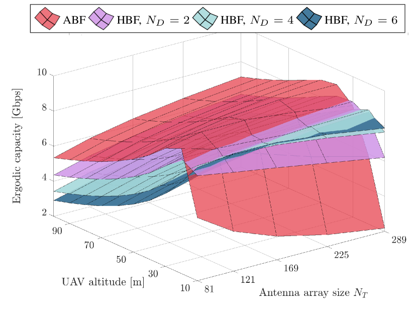
Fig. 9: Ergodic capacity of ABF and HBF vs. the deployment altitude, the antenna array size, and the number of parallel beams in HBF, when $\lambda_{u}=0.05$ GU/m².

The GU density is another key parameter of the network. Along these lines, Fig. 10 illustrates the ergodic capacity of the ABF and HBF architectures for different values of $\lambda_{u}$. We clearly see that ABF’s capacity drops when $\lambda_{u}$ decreases. The reasons are twofold. First, considering sparser networks, Eq. (34) demonstrates that the distance to the serving UAV increases, which results in weaker channels. Second, when fewer GUs are deployed, the probability that they will be placed within the coverage of the single VB decreases accordingly. In this perspective, an HBF configuration has the potential to guarantee better capacity by making it possible for the (sparse) GUs to still maintain connectivity with one of the available TBs: the performance gap grows proportionally with $N_{D}$, since more parallel TBs result in more connectivity opportunities for the GUs. Fig. 10 also demonstrates that the altitude for which the peak value is reached increases as $\lambda_{u}$ decreases: this approach (i) offers better signal quality by increasing the LOS probability (which has, therefore, a more significant impact than the resulting larger path loss), and (ii) produces larger VBs (which generate larger coverage regions).

VI-D Final Comments and Design Guidelines

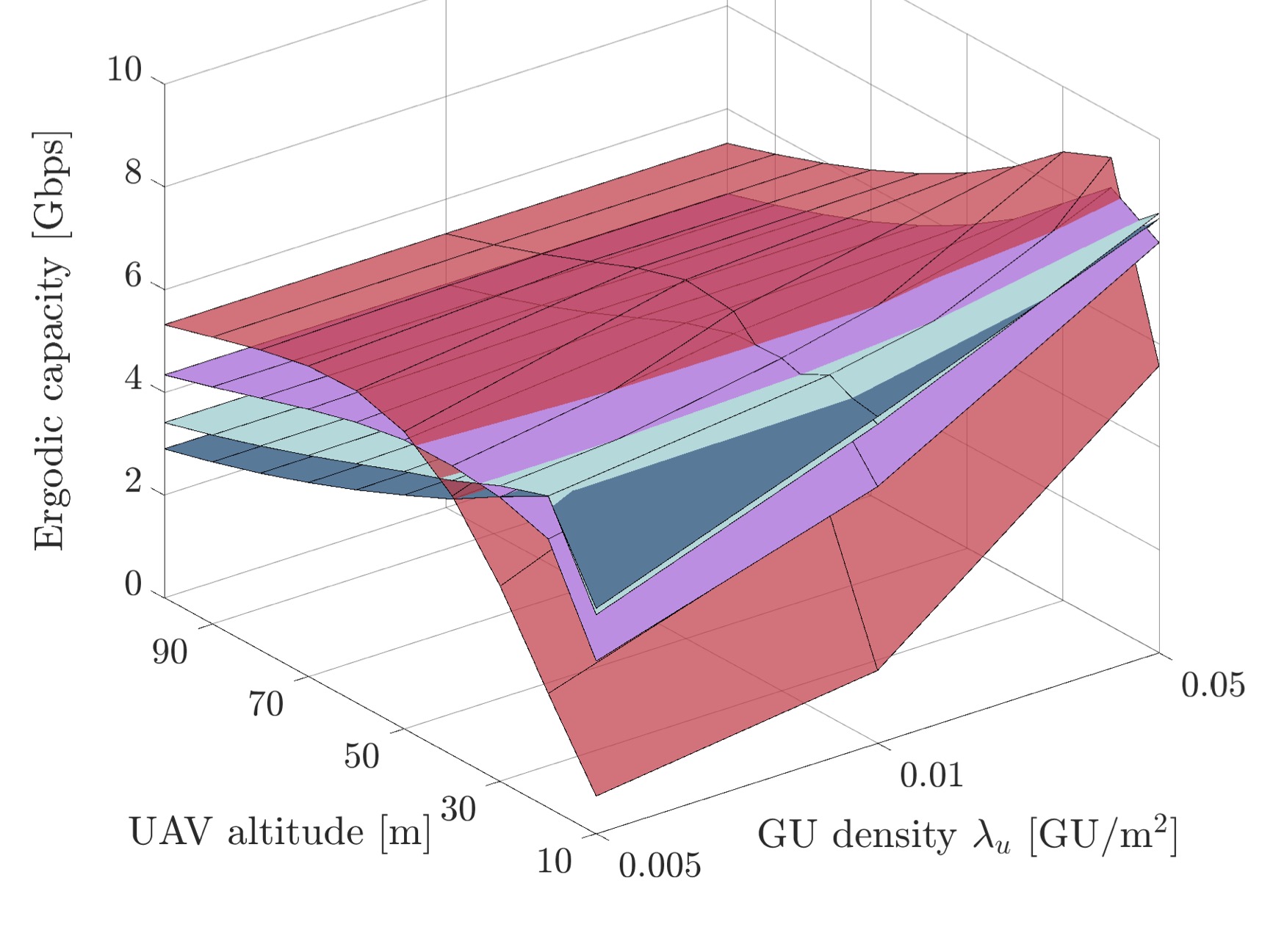
(a) Antenna array size $N_{T}=9\times 9$.

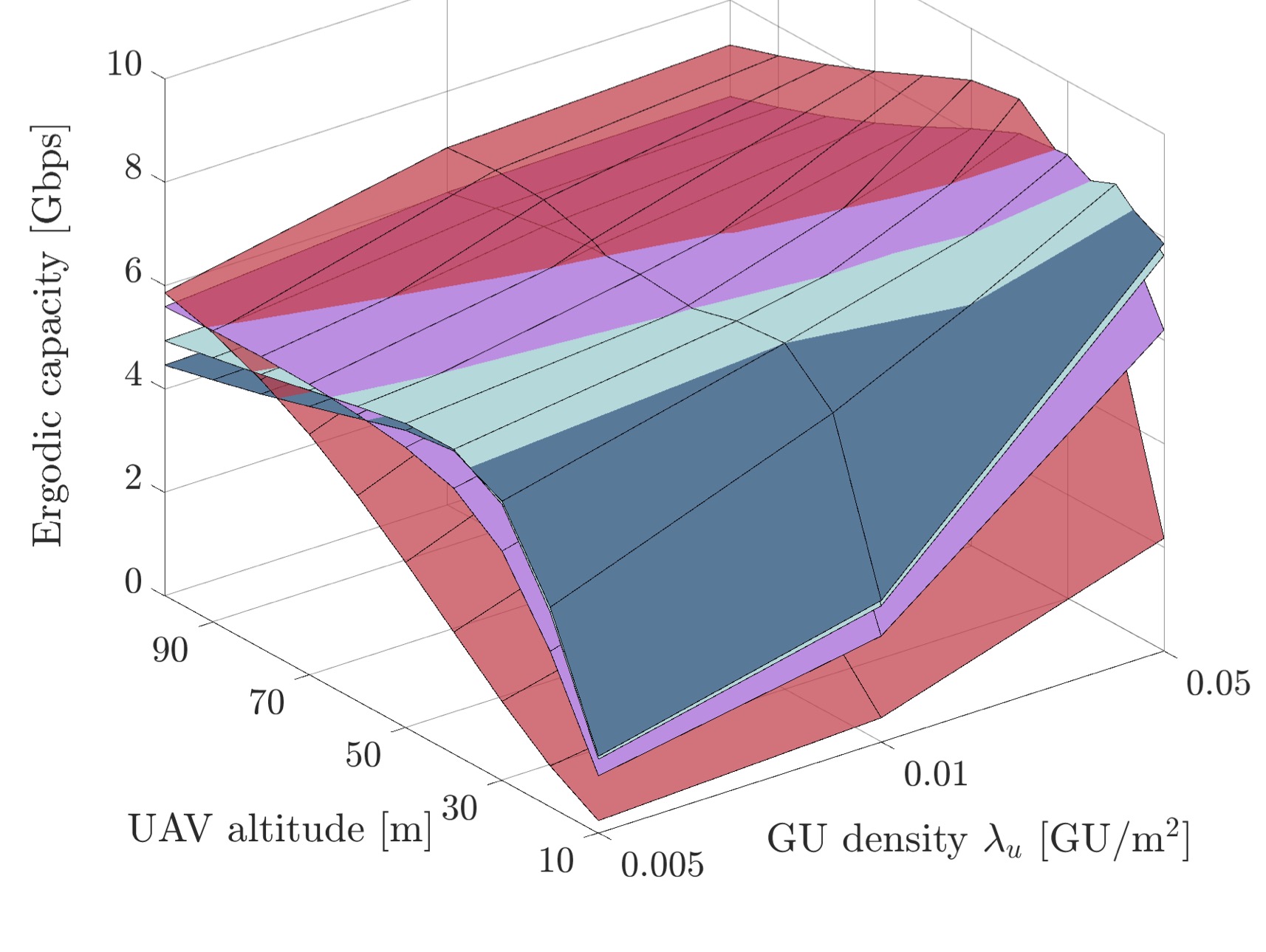
(b) Antenna array size $N_{T}=17\times 17$.

Fig. 10: Ergodic capacity of ABF and HBF vs. the deployment altitude, the antenna array size, the number of parallel beams in HBF, and the GU’s deployment density.

Based on the results we presented in the previous subsections, we now provide some guidelines to optimally dimension a UAV-operated network at mmWave frequencies to jointly optimize power consumption and ergodic capacity.

ABF vs. HBF. In general, ABF provides the highest ergodic capacity since the transmit power is concentrated towards a single vertical beam, while HBF can minimize the total power consumption when $N_{D}>1$ by reducing the number of UAVs that need to be deployed to achieve full service coverage. However, it should be noted that the capacity degradation for HBF is quite limited (e.g., only $-6\%$ for $N_{T}=9\times 9$ and $N_{D}=2$ at $h^{*}=25$ m, as illustrated in Fig. 8), in the face of a performance improvement in terms of power consumption by $60\%$ (as depicted in Fig. 6), thus making HBF an attractive option. Moreover, Fig. 11 illustrates that HBF guarantees better power efficiency, which is computed as $\tau_{i}/P_{C}^{i}$, $i\in\{\rm ABF,HBF\}$, in sparse deployments (i.e., $\lambda_{u}=0.005$ GU/m², which identify a typical emergency situation in public safety scenarios) for all investigated configurations, by offering the GUs more connectivity opportunities through tilted beams. Fig. 11(b) also exemplifies that HBF outperforms ABF when decreasing the UAV altitude, and when increasing the antenna array size (which is required to serve the traffic of the farthest GUs through the resulting higher gain achieved by beamforming).

(a) $\lambda_{u}=0.005$ GU/m² and $N_{T}=13\times 13$.

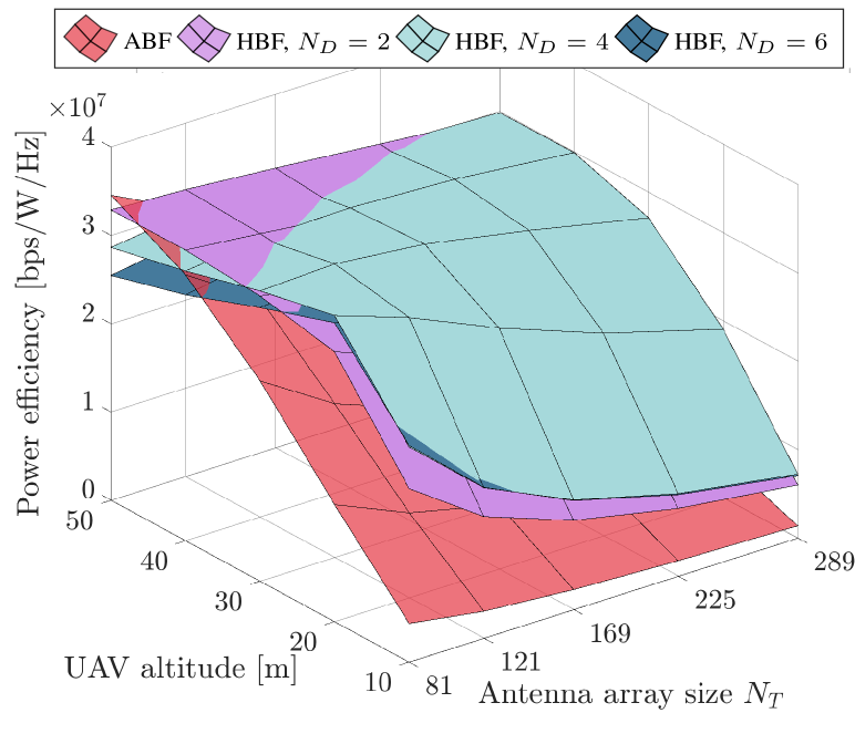
(b) $\lambda_{u}=0.005$ GU/m².

Fig. 11: Power efficiency of ABF and HBF vs. the deployment altitude, the number of parallel beams in HBF, and $N_{T}$.

Impact of $h$. From a theoretical point of view, it would be preferable to increase the deployment altitude to expand the service region shaped by VBs and TBs on the ground, and consistently reduce the number of UAVs that are required to cover the AoI. In practice, there exists an optimal value $h^{*}$ that maximizes the ergodic capacity: for $h>h^{*}$, despite the more likely LOS links, the impact of the increased path loss between the GUs and the serving UAV reduces the overall link budget, thus leading to intermittent connectivity. Notably, the value of $h^{*}$ increases as $\lambda_{u}$ decreases, especially when ABF is implemented. For example, Fig. 10(a) shows that, for $N_{T}=9\times 9$, $h^{*}$ moves from $60$ m when $\lambda_{u}=0.005$ GU/m² to $30$ m when $\lambda_{u}=0.05$ GU/m².

Impact of $N_{D}$ and $N_{RF}$. HBF permits to form $N_{D}$ parallel beams to serve multiple GUs simultaneously from the same UAV station. This approach (i) guarantees reduced power consumption compared to ABF, and (ii) offers higher ergodic capacity when UAVs hover at low altitude. Nevertheless, $N_{D}$ exhibits a maximum, that is inversely proportional to the GU density $\lambda_{u}$, above which increasing the number of TBs would deteriorate the ergodic capacity (as the transmit power has to be split among more directions simultaneously) with limited performance improvements in terms of power consumption. Finally, the optimal design would be to set $N_{D}=N_{RF}$.

Impact of $N_{T}$. In general, $N_{T}$ should be reduced as much as possible. Not only can this strategy minimize the total power consumption (by reducing the number of electronic components in the RF chain(s)), but it can also improve the ergodic capacity by allowing UAVs to generate larger connectivity regions on the ground. However, $N_{T}$ might still need to be increased, despite the higher power consumption, to provide connectivity (i) when $h$ is large, or (ii) when $\lambda_{u}$ is small, i.e., when the distance to the serving UAV increases. For example, from Fig. 8 we can see that the ergodic capacity grows by more than $30\%$ when $N_{T}$ is increased from $9\times 9$ to $17\times 17$ at $h=100$ m.

VII Conclusions and Future Work

In this work we characterized the ergodic capacity and power consumption of UAV mmWave networks and investigated the relationship between UAV altitude, GU density, and antenna design. Our model takes into account the power consumed by both UAV’s hovering and communication hardware components, and derives an analytical expression of the ergodic capacity for ABF and HBF architectures. We validated our analytical curves via Monte Carlo simulations, and demonstrated that there exists an optimal altitude at which the UAV should be placed to improve network capacity, which depends on the GU density and the adopted beamforming architecture. Specifically, we showed that HBF always consumes the least power, especially when increasing the antenna array size, with minimum capacity degradation compared to ABF. Moreover, the hybrid approach outperforms ABF in terms of capacity too when considering sparse GU deployments and when the UAVs hover at low altitudes (e.g., during take off or when civil flight authorities pose a limit on the height of the UAV).

This work opens up some particularly interesting research directions, such as the definition of a hybrid mechanism able to dynamically identify the recommended network configuration(s) as a function of the UAV swarm size, altitude, and antenna architecture. We will also investigate how to practically integrate UAVs with other non-terrestrial platforms like HAPs or satellites to promote ubiquitous and high-capacity global connectivity to on-the-ground devices.

Appendix A Proof of Theorem 2

With the assumption that the small scale fading is modeled as a Nakagami-m random variable $\gamma_{i}$ with parameter _i and $\Omega_{i}$, $i\in\{L,N\}$, for a given constant $x>0$, the probability $\mathbb{P}[\gamma_{i}>x]$ can be written as

$$\mathbb{P}[\gamma_{i}>x] =1-\mathbb{P}[\gamma_{i}\leq x]$$

$$=1-P\left(m_{i},\frac{m_{i}}{\Omega_{i}}x^{2}\right)$$

$$=1-\frac{u\left(m_{i},\frac{m_{i}}{\Omega_{i}}x^{2}\right)}{\Gamma(m_{i})}$$

$$=1-\frac{\int_{0}^{\frac{m_{i}}{\Omega_{i}}x}l^{m_{i}-1}e^{-l}dl}{(m_{i}-1)!}$$ (42)

where $P(m_{i},\frac{m_{i}}{\Omega_{i}}x^{2})$ is the (regularized) incomplete gamma function, and $u(m_{i},\frac{m_{i}}{\Omega_{i}}x^{2})$ is the lower incomplete gamma function. Let $r_{1}$ be the 2D distance between the UAV and the closest GU $\in\Phi_{u}$ within the VB, whose pdf is expressed in Eq. (34). The ergodic capacity experienced from the GU in the VB can be rewritten from Eq. (36) as

$$\tau^{\rm VB}\overset{\Delta}{=}\mathbb{E}_{\Phi_{u}}\left[B\log_{2}(1+\text{SNR}(r))\right]$$

$$=\int_{0}^{r_{\rm VB}}Bf_{r1}^{\rm VB}(r)\mathbb{E}_{\Phi_{u}}\left\{\log_{2}\left(1+\frac{P_{t}G\gamma_{L}p_{L}(r)\ell_{L}(r)}{N_{D}\cdot\mathrm{NF}\cdot\sigma^{2}}\right.\right.$$

$$\left.\left.+\frac{P_{t}G\gamma_{N}p_{N}(r)\ell_{N}(r)}{N_{D}\cdot\mathrm{NF}\cdot\sigma^{2}}\right)\right\}\mathrm{d}r$$

$$\overset{(a)}{=}\int_{0}^{r_{\rm VB}}\int_{0}^{\infty}Bf_{r_{1}}^{\rm VB}(r)\mathbb{P}[\gamma_{L}>\beta(t,\gamma_{N})]\mathrm{d}t\mathrm{d}r$$

$$\overset{(b)}{=}\int_{0}^{r_{\rm VB}}\int_{0}^{\infty}Bf_{r_{1}}^{\rm VB}(r)\mathbb{E}_{\Phi_{u,N}}\left[1-\frac{\int_{0}^{\Delta_{L}}l^{m_{L}-1}e^{-l}dl}{(m_{L}-1)!}\right]\mathrm{d}t\mathrm{d}r$$

$$\overset{(c)}{=}\int_{0}^{r_{\rm VB}}\int_{0}^{\infty}\left(1+\frac{\mathbb{E}_{\Phi_{u,N}}\left[\left(\frac{l^{m_{L}}}{l}+\sum\limits_{j=2}^{m_{L}}\frac{\Gamma(m_{L})}{(m_{L}-j)!}l^{m_{L}-j}\right)e^{-l}\Big{|}_{0}^{\Delta_{L}}\right]}{(m_{L}-1)!}\right)$$

$$\cdot Bf_{r_{1}}^{\rm VB}(r)\mathrm{d}t\mathrm{d}r$$

$$=\int_{0}^{r_{\rm VB}}\int_{0}^{\infty}\frac{\mathbb{E}_{\Phi_{u,N}}\left[\left(l^{m_{L}-1}+\sum\limits_{j=2}^{m_{L}}\frac{\Gamma(m_{L})}{(m_{L}-j)!}l^{m_{L}-j}\right)e^{-\Delta_{L}}\right]}{(m_{L}-1)!}$$

$$\cdot Bf_{r_{1}}^{\rm VB}(r)\mathrm{d}t\mathrm{d}r$$

$$=B\int_{0}^{r_{\rm VB}}\int_{0}^{\infty}\int_{0}^{\infty}\frac{\left(l^{m_{L}-1}+\sum\limits_{j=2}^{m_{L}}\frac{\Gamma(m_{L})}{(m_{L}-j)!}l^{m_{L}-j}\right)e^{-\Delta_{L}}}{(m_{L}-1)!}$$

$$\cdot f_{r_{1}}^{\rm VB}(r)p_{\gamma}(\gamma_{N})\mathrm{d}\gamma_{N}\mathrm{d}t\mathrm{d}r,$$ (43)

where $(a)$ follows the fact that, for a positive random variable X, $\mathbb{E}(X)=\int_{t>0}\mathbb{P}(X>t)\mathrm{d}t$ [58], $(b)$ is obtained from Eq. (42), and $(c)$ derives from

$$\int_{0}^{\Delta_{L}}l^{m_{L}-1}e^{-l}dl$$

$$=-(l^{m_{L}-1}+\sum_{j=2}^{m_{L}}\frac{\Gamma(m_{L})}{(m_{L}-j)}l^{m_{L}-j})e^{-l}\Big{|}_{0}^{\Delta_{L}}.$$ (44)

In Eq. (43), $p_{\gamma}(\gamma_{N})$ is the probability distribution of the Nakagami-m small-scale fading for NLOS propagation, and we assumed

$$\beta(t,\gamma_{N})=\frac{(e^{t\ln 2}-1)N_{D}\mathrm{NF}\sigma^{2}-P_{t}G\gamma_{N}p_{N}(r)\ell_{N}(r)}{P_{t}Gp_{L}(r)\ell_{L}(r)},$$ (45)

$$\Delta_{L}=\frac{m_{L}}{\Omega_{L}}\beta(t,\gamma_{N}).$$ (46)

References

- [1] F. Khan, “Multi-comm-core architecture for terabit-per-second wireless,” IEEE Communications Magazine, vol. 54, no. 4, pp. 124–129, Apr 2016.
- [2] M. Giordani, M. Polese, M. Mezzavilla, S. Rangan, and M. Zorzi, “Toward 6G Networks: Use Cases and Technologies,” IEEE Communications Magazine, vol. 58, no. 3, Mar. 2020.
- [3] A. Chaoub, M. Giordani, B. Lall, V. Bhatia, A. Kliks, L. Mendes, K. Rabie, H. Saarnisaari, A. Singhal, N. Zhang et al., “6G for Bridging the Digital Divide: Wireless Connectivity to Remote Areas,” 2020, submitted to the IEEE Wireless Communications Magazine, 2020. [Online]. Available: https://arxiv.org/abs/2009.04175
- [4] M. Giordani and M. Zorzi, “Non-Terrestrial Networks in the 6G Era: Challenges and Opportunities,” submitted to IEEE Network, 2020. [Online]. Available: https://arxiv.org/abs/1912.10226
- [5] ——, “Satellite Communication at Millimeter Waves: a Key Enabler of the 6G Era,” IEEE International Conference on Computing, Networking and Communications (ICNC), Feb 2020.
- [6] B. Li, Z. Fei, and Y. Zhang, “UAV communications for 5G and beyond: Recent advances and future trends,” IEEE Internet of Things Journal, vol. 6, no. 2, pp. 2241–2263, Apr 2018.
- [7] Y. Zeng, R. Zhang, and T. J. Lim, “Wireless communications with unmanned aerial vehicles: opportunities and challenges,” IEEE Communications Magazine, vol. 54, no. 5, pp. 36–42, May 2016.
- [8] L. Zhang, H. Zhao, S. Hou, Z. Zhao, H. Xu, X. Wu, Q. Wu, and R. Zhang, “A Survey on 5G Millimeter Wave Communications for UAV-Assisted Wireless Networks,” IEEE Access, vol. 7, pp. 117 460–117 504, Jul 2019.
- [9] X. Li, H. Yao, J. Wang, X. Xu, C. Jiang, and L. Hanzo, “A Near-Optimal UAV-Aided Radio Coverage Strategy for Dense Urban Areas,” IEEE Transactions on Vehicular Technology, vol. 68, no. 9, pp. 9098–9109, Jul 2019.
- [10] M. Xiao, S. Mumtaz, Y. Huang, L. Dai, Y. Li, M. Matthaiou, G. K. Karagiannidis, E. Björnson, K. Yang, C. I, and A. Ghosh, “Millimeter Wave Communications for Future Mobile Networks,” IEEE Journal on Selected Areas in Communications, vol. 35, no. 9, pp. 1909–1935, Jun 2017.
- [11] M. Gapeyenko, V. Petrov, D. Moltchanov, S. Andreev, N. Himayat, and Y. Koucheryavy, “Flexible and Reliable UAV-Assisted Backhaul Operation in 5G mmWave Cellular Networks,” IEEE Journal on Selected Areas in Communications, vol. 36, no. 11, pp. 2486–2496, Oct 2018.
- [12] N. Tafintsev, D. Moltchanov, M. Gerasimenko, M. Gapeyenko, J. Zhu, S. Yeh, N. Himayat, S. Andreev, Y. Koucheryavy, and M. Valkama, “Aerial Access and Backhaul in mmWave B5G Systems: Performance Dynamics and Optimization,” IEEE Communications Magazine, vol. 58, no. 2, pp. 93–99, Feb 2020.
- [13] M. Giordani, M. Polese, A. Roy, D. Castor, and M. Zorzi, “A Tutorial on Beam Management for 3GPP NR at mmWave Frequencies,” IEEE Communications Surveys Tutorials, vol. 21, no. 1, pp. 173–196, Firstquarter 2019.
- [14] S. Sun, T. S. Rappaport, R. W. Heath, A. Nix, and S. Rangan, “MIMO for millimeter-wave wireless communications: beamforming, spatial multiplexing, or both?” IEEE Communications Magazine, vol. 52, no. 12, pp. 110–121, Dec. 2014.
- [15] C. G. Tsinos, S. Maleki, S. Chatzinotas, and B. Ottersten, “On the energy-efficiency of hybrid analog–digital transceivers for single- and multi-carrier large antenna array systems,” IEEE Journal on Selected Areas in Communications, vol. 35, no. 9, pp. 1980–1995, Jun. 2017.
- [16] Z. Xiao, H. Dong, L. Bai, D. O. Wu, and X. Xia, “Unmanned Aerial Vehicle Base Station (UAV-BS) Deployment With Millimeter-Wave Beamforming,” IEEE Internet of Things Journal, vol. 7, no. 2, pp. 1336–1349, Feb 2020.
- [17] F. Sohrabi and W. Yu, “Hybrid analog and digital beamforming for mmWave OFDM large-scale antenna arrays,” IEEE Journal on Selected Areas in Communications, vol. 35, no. 7, pp. 1432–1443, Apr 2017.
- [18] A. F. Molisch, V. V. Ratnam, S. Han, Z. Li, S. L. H. Nguyen, L. Li, and K. Haneda, “Hybrid beamforming for massive MIMO: A survey,” IEEE Communications Magazine, vol. 55, no. 9, pp. 134–141, Sep 2017.
- [19] V. V. C. Ravi and H. S. Dhillon, “Downlink coverage probability in a finite network of unmanned aerial vehicle (UAV) base stations,” in IEEE 17th International Workshop on Signal Processing Advances in Wireless Communications (SPAWC), 2016.
- [20] V. V. Chetlur and H. S. Dhillon, “Downlink coverage analysis for a finite 3-D wireless network of unmanned aerial vehicles,” IEEE Transactions on Communications, vol. 65, no. 10, pp. 4543–4558, Oct. 2017.
- [21] W. Yi, Y. Liu, M. Elkashlan, and A. Nallanathan, “Modeling and coverage analysis of downlink UAV networks with mmWave communications,” in 2019 IEEE International Conference on Communications Workshops (ICC Workshops). IEEE, 2019, pp. 1–6.
- [22] M. Boschiero, M. Giordani, M. Polese, and M. Zorzi, “Coverage Analysis of UAVs in Millimeter Wave Networks: A Stochastic Geometry Approach,” in 2020 International Wireless Communications and Mobile Computing (IWCMC), 2020, pp. 351–357.
- [23] C. Di Franco and G. Buttazzo, “Energy-aware coverage path planning of UAVs,” in IEEE International Conference on Autonomous Robot Systems and Competitions, 2015.
- [24] S. Naqvi, J. Chakareski, N. Mastronarde, J. Xu, F. Afghah, and A. Razi, “Energy efficiency analysis of UAV-assisted mmWave HetNets,” in IEEE International Conference on Communications (ICC), 2018.
- [25] Z. Xiao, P. Xia, and X. Xia, “Enabling UAV cellular with millimeter-wave communication: Potentials and approaches,” IEEE Communications Magazine, vol. 54, no. 5, pp. 66–73, May 2016.
- [26] W. Xia, M. Polese, M. Mezzavilla, G. Loianno, S. Rangan, and M. Zorzi, “Millimeter Wave Remote UAV Control and Communications for Public Safety Scenarios,” in Proc. of the 1st Intl. Workshop on Internet of Autonomous Unmanned Vehicles, ser. IAUV ’19, Boston, MA, 2019.
- [27] J. Zhao, G. Gao, L. Kuang, Q. Wu, and W. Jia, “Channel tracking with flight control system for UAV mmWave MIMO communications,” IEEE Communications Letters, vol. 22, no. 6, pp. 1224–1227, Jun. 2018.
- [28] M. M. Azari, Y. Murillo, O. Amin, F. Rosas, M.-S. Alouini, and S. Pollin, “Coverage maximization for a poisson field of drone cells,” in IEEE 28th Annual International Symposium on Personal, Indoor, and Mobile Radio Communications (PIMRC), 2017.
- [29] C. Liu, M. Ding, C. Ma, Q. Li, Z. Lin, and Y.-C. Liang, “Performance analysis for practical unmanned aerial vehicle networks with LoS/NLoS transmissions,” in IEEE International Conference on Communications Workshops (ICC Workshops), 2018.
- [30] W. Yi, Y. Liu, E. Bodanese, A. Nallanathan, and G. K. Karagiannidis, “A Unified Spatial Framework for UAV-Aided MmWave Networks,” IEEE Transactions on Communications, vol. 67, no. 12, pp. 8801–8817, Oct 2019.
- [31] X. Wang and M. C. Gursoy, “Coverage Analysis for Energy-Harvesting UAV-Assisted mmWave Cellular Networks,” IEEE Journal on Selected Areas in Communications, vol. 37, no. 12, pp. 2832–2850, Oct 2019.
- [32] A. Colpaert, E. Vinogradov, and S. Pollin, “Aerial coverage analysis of cellular systems at LTE and mmwave frequencies using 3D city models,” Sensors, vol. 18, no. 12, p. 4311, Dec 2018.
- [33] L. Zhu, J. Zhang, Z. Xiao, X. Cao, X. Xia, and R. Schober, “Millimeter-Wave Full-Duplex UAV Relay: Joint Positioning, Beamforming, and Power Control,” IEEE Journal on Selected Areas in Communications, vol. 38, no. 9, pp. 2057–2073, Jan 2020.
- [34] Z. Xiao, H. Dong, L. Bai, D. O. Wu, and X. Xia, “Unmanned Aerial Vehicle Base Station (UAV-BS) Deployment With Millimeter-Wave Beamforming,” IEEE Internet of Things Journal, vol. 7, no. 2, pp. 1336–1349, Feb 2020.
- [35] M. Mozaffari, W. Saad, M. Bennis, and M. Debbah, “Drone small cells in the clouds: Design, deployment and performance analysis,” in IEEE Global Communications Conference (GLOBECOM), 2015.
- [36] D. Yang, Q. Wu, Y. Zeng, and R. Zhang, “Energy tradeoff in ground-to-UAV communication via trajectory design,” IEEE Transactions on Vehicular Technology, vol. 67, no. 7, pp. 6721–6726, Mar. 2018.
- [37] Y. Zeng, J. Xu, and R. Zhang, “Energy minimization for wireless communication with rotary-wing UAV,” IEEE Transactions on Wireless Communications, vol. 18, no. 4, pp. 2329–2345, Apr. 2019.
- [38] O. Orhan, E. Erkip, and S. Rangan, “Low power analog-to-digital conversion in millimeter wave systems: Impact of resolution and bandwidth on performance,” in Information Theory and Applications Workshop (ITA), 2015.
- [39] S. Buzzi and C. D’Andrea, “Energy efficiency and asymptotic performance evaluation of beamforming structures in doubly massive MIMO mmWave systems,” IEEE Transactions on Green Communications and Networking, vol. 2, no. 2, pp. 385–396, Jan. 2018.
- [40] W. Miao, C. Luo, G. Min, L. Wu, T. Zhao, and Y. Mi, “Position-Based Beamforming Design for UAV Communications in LTE Networks,” in IEEE International Conference on Communications (ICC), 2019.
- [41] L. Yang and W. Zhang, “Beam tracking and optimization for UAV communications,” IEEE Transactions on Wireless Communications, vol. 18, no. 11, pp. 5367–5379, Nov. 2019.
- [42] W. Miao, C. Luo, G. Min, and Z. Zhao, “Lightweight 3-d beamforming design in 5g uav broadcasting communications,” IEEE Transactions on Broadcasting, vol. 66, no. 2, pp. 515–524, Jun 2020.
- [43] S. Li, B. Duo, X. Yuan, Y.-C. Liang, and M. Di Renzo, “Reconfigurable intelligent surface assisted UAV communication: Joint trajectory design and passive beamforming,” IEEE Wireless Communications Letters, vol. 9, no. 5, pp. 716–720, May 2020.
- [44] Q. Yu, C. Han, J. Wang, and L. Bai, “Low Complexity Hybrid Beamforming for MmWave-UAV Communication Systems with a Pre-defined Codebook,” in Proceedings of the 2nd International Conference on Control and Computer Vision, 2019.
- [45] H. Ren, L. Li, W. Xu, W. Chen, and Z. Han, “Machine learning-based hybrid precoding with robust error for UAV mmWave massive MIMO,” in IEEE International Conference on Communications (ICC), 2019.
- [46] ITU, “Propagation data and prediction methods for the design of terrestrial broadband millimetric radio access systems,” P.1410-2, 2003.
- [47] A. Al-Hourani, S. Kandeepan, and S. Lardner, “Optimal LAP altitude for maximum coverage,” IEEE Wireless Communications Letters, vol. 3, no. 6, pp. 569–572, Jul. 2014.
- [48] M. Mozaffari, W. Saad, M. Bennis, and M. Debbah, “Unmanned aerial vehicle with underlaid device-to-device communications: Performance and tradeoffs,” IEEE Transactions on Wireless Communications, vol. 15, no. 6, pp. 3949–3963, Feb. 2016.
- [49] T. S. Rappaport, S. Sun, R. Mayzus, H. Zhao, Y. Azar, K. Wang, G. N. Wong, J. K. Schulz, M. Samimi, and F. Gutierrez, “Millimeter Wave Mobile Communications for 5G Cellular: It Will Work!” IEEE Access, vol. 1, pp. 335–349, May 2013.
- [50] Y. Zhu, G. Zheng, and M. Fitch, “Secrecy Rate Analysis of UAV-Enabled mmWave Networks Using Matern Hardcore Point Processes,” IEEE Journal on Selected Areas in Communications, vol. 36, no. 7, pp. 1397–1409, Jul. 2018.
- [51] M. Nakagami, “The m-distribution—a general formula of intensity distribution of rapid fading,” in Statistical methods in radio wave propagation. Elsevier, 1960, pp. 3–36.
- [52] M. T. Dabiri, H. Safi, S. Parsaeefard, and W. Saad, “Analytical channel models for millimeter wave UAV networks under hovering fluctuations,” IEEE Transactions on Wireless Communications, vol. 19, no. 4, pp. 2868–2883, Feb. 2020.
- [53] X. Yu, J. Zhang, M. Haenggi, and K. B. Letaief, “Coverage analysis for millimeter wave networks: The impact of directional antenna arrays,” IEEE Journal on Selected Areas in Communications, vol. 35, no. 7, pp. 1498–1512, Jul 2017.
- [54] C. A. Balanis, Antenna theory: analysis and design. John Wiley & Sons, 2016.
- [55] Z. Liu, R. Sengupta, and A. Kurzhanskiy, “A power consumption model for multi-rotor small unmanned aircraft systems,” in International Conference on Unmanned Aircraft Systems (ICUAS), 2017.
- [56] W. B. Abbas, F. Gomez-Cuba, and M. Zorzi, “Millimeter Wave Receiver Efficiency: A Comprehensive Comparison of Beamforming Schemes With Low Resolution ADCs,” IEEE Transactions on Wireless Communications, vol. 16, no. 12, pp. 8131–8146, Dec 2017.
- [57] L. N. Ribeiro, S. Schwarz, M. Rupp, and A. L. F. de Almeida, “Energy Efficiency of mmWave Massive MIMO Precoding With Low-Resolution DACs,” IEEE Journal of Selected Topics in Signal Processing, vol. 12, no. 2, pp. 298–312, May 2018.
- [58] J. G. Andrews, F. Baccelli, and R. K. Ganti, “A Tractable Approach to Coverage and Rate in Cellular Networks,” IEEE Transactions on Communications, vol. 59, no. 11, pp. 3122–3134, Nov. 2011.
- [59] D. Pepe and D. Zito, “A 78.8–92.8 GHz 4-bit 0–360 active phase shifter in 28nm FDSOI CMOS with 2.3 dB average peak gain,” in 41st European Solid-State Circuits Conference (ESSCIRC), 2015.
- [60] K. Scheir, S. Bronckers, J. Borremans, P. Wambacq, and Y. Rolain, “A 52 GHz Phased-Array Receiver Front-End in 90 nm Digital CMOS,” IEEE Journal of Solid-State Circuits, vol. 43, no. 12, pp. 2651–2659, Dec. 2008.
- [61] Y. Yu, P. G. Baltus, A. de Graauw, E. van der Heijden, C. S. Vaucher, and A. H. van Roermund, “A 60 GHz phase shifter integrated with LNA and PA in 65 nm CMOS for phased array systems,” IEEE Journal of Solid-State Circuits, vol. 45, no. 9, pp. 1697–1709, Aug 2010.
- [62] M. Kraemer, D. Dragomirescu, and R. Plana, “Design of a very low-power, low-cost 60 GHz receiver front-end implemented in 65 nm CMOS technology,” International Journal of Microwave and Wireless Technologies, vol. 3, no. 2, pp. 131–138, Apr. 2011.
- [63] X. Yu, J. Zhang, M. Haenggi, and K. B. Letaief, “Coverage Analysis for Millimeter Wave Networks: The Impact of Directional Antenna Arrays,” IEEE Journal on Selected Areas in Communications, vol. 35, no. 7, pp. 1498–1512, Apr 2017.
- [64] C. Marcu, “LO Generation and Distribution for 60GHz Phased Array Transceivers,” Ph.D. dissertation, EECS Department, University of California, Berkeley, Dec 2011.
- [65] S. Rangan, T. Rappaport, E. Erkip, Z. Latinovic, M. R. Akdeniz, and Y. Liu, “Energy efficient methods for millimeter wave picocellular systems,” in IEEE Communication Theory Workshop, 2013.
- [66] R. Méndez-Rial, C. Rusu, N. González-Prelcic, A. Alkhateeb, and R. W. Heath, “Hybrid MIMO architectures for millimeter wave communications: Phase shifters or switches?” IEEE Access, vol. 4, pp. 247–267, Jan. 2016.
- [67] Y. Zhu, G. Zheng, and M. Fitch, “Secrecy rate analysis of uav-enabled mmwave networks using matérn hardcore point processes,” IEEE Journal on Selected Areas in Communications, vol. 36, no. 7, pp. 1397–1409, 2018.
- [68] M. R. Akdeniz, Y. Liu, M. K. Samimi, S. Sun, S. Rangan, T. S. Rappaport, and E. Erkip, “Millimeter Wave Channel Modeling and Cellular Capacity Evaluation,” IEEE Journal on Selected Areas in Communications, vol. 32, no. 6, pp. 1164–1179, Jun. 2014.
- [69] M. Navolio, “Public Safety Wireless Data Network Requirements Project,” in Needs Assessment Report, 2011.
- [70] M. Giordani and M. Zorzi, “Improved user tracking in 5G millimeter wave mobile networks via refinement operations,” in 16th Annual Mediterranean Ad Hoc Networking Workshop (Med-Hoc-Net), 2017.
- [71] T. McElvaney, “5G: From a Public Safety Perspective,” 2015. [Online]. Available: http://www.atis.org/5g/presentations/5G_PublicSafety_TMcElvaney.pdf