BIMODAL BEHAVIOR AND CONVERGENCE REQUIREMENT IN MACROSCOPIC PROPERTIES
OF THE MULTIPHASE INTERSTELLAR MEDIUM FORMED BY ATOMIC CONVERGING FLOWS

Abstract

We systematically perform hydrodynamics simulations of 20 ${\rm km\,s^{-1}}$ converging flows of the warm neutral medium (WNM) to calculate the formation of the cold neutral medium (CNM), especially focusing on the mean properties of the multiphase interstellar medium (ISM), such as the average shock front position and the mean density on a 10 pc scale. Our results show that the convergence in those mean properties requires 0.02 pc spatial resolution that resolves the cooling length of the thermally unstable neutral medium (UNM) to follow the dynamical condensation from the WNM to CNM. We also find that two distinct post-shock states appear in the mean properties depending on the amplitude of the upstream WNM density fluctuation $\Delta\rho_{0}$ ($=\sqrt{\langle\delta\rho_{0}^{2}\rangle}/\rho_{0}$). When $\Delta\rho_{0}>10$ %, the interaction between shocks and density inhomogeneity leads to a strong driving of the post-shock turbulence of $>3$ km s^-1, which dominates the energy budget in the shock-compressed layer. The turbulence prevents the dynamical condensation by cooling and the following CNM formation, and the CNM mass fraction remains as $\sim 45$ %. In contrast, when $\Delta\rho_{0}\leq 10$ %, the shock fronts maintain an almost straight geometry and CNM formation efficiently proceeds, resulting in the CNM mass fraction of $\sim 70$ %. The velocity dispersion is limited to the thermal-instability mediated level of $\sim 2$ – $3$ km s^-1 and the layer is supported by both turbulent and thermal energy equally. We also propose an effective equation of state that models the multiphase ISM formed by the WNM converging flow as a one-phase ISM.

1 Introduction

Molecular clouds are formation sites of stars (Kennicutt & Evans 2012) and the formation process of molecular clouds is essential to understand the initial condition of star formation. Since the galactic disks are largely occupied by the warm neutral medium (WNM: $\simeq$ 6000 K and $\simeq$ 1 ${\rm cm^{-3}}$), the phase transition from the WNM to the cold neutral medium (CNM: $\simeq$ 100 K and $\simeq$ 100 ${\rm cm^{-3}}$) is the initial step in the formation of molecular clouds ($\simeq$ 10 K and $\geq$ 100 ${\rm cm^{-3}}$). The thermal instability due to radiative cooling and heating significantly influences this phase transition dynamics (Field 1965; Field et al. 1969; Zel’dovich & Pikel’ner 1969; Wolfire et al. 1995, 2003), and is believed to be triggered by supersonic flows originated in supernovae (McKee & Ostriker 1977; Chevalier 1977, 1999), superbubbles (McCray & Snow 1979; Tomisaka et al. 1981; Tomisaka & Ikeuchi 1986; Kim et al. 2017; Ntormousi et al. 2017), galactic spirals (Shu et al. 1972; Wada et al. 2011; Baba et al. 2017; Kim et al. 2020), and galaxy mergers (Heitsch et al. 2006; Arata et al. 2018).

Many authors have studied the dynamical condensation through the thermal instability in a shock-compressed layer formed by supersonic converging flows, whose importance is initially highlighted with one-dimensional simulations (e.g., Hennebelle & Pérault 1999; Koyama & Inutsuka 2000). This converging-flow configuration is a technical analogue to easily calculate the thermal instability in the post-shock rest frame, instead of tracking the post-shock interstellar medium (ISM) propagating with a shock front in space (see Koyama & Inutsuka 2000). Multi-dimensional simulations are later performed in two dimensions (Koyama & Inutsuka 2002; Audit & Hennebelle 2005; Heitsch et al. 2005; Hennebelle & Audit 2007) and in three dimensions (Heitsch et al. 2006; Vázquez-Semadeni et al. 2006, 2007; Audit & Hennebelle 2008). They essentially form the multiphase ISM with supersonic turbulence consistent with observations (e.g., Larson 1981; Heyer & Brunt 2004). There have been also converging-flow studies that extensively investigate the effect of magnetic fields (Hennebelle & Pérault 2000; Inoue & Inutsuka 2008, 2009; Hennebelle et al. 2008; Heitsch et al. 2009; Vázquez-Semadeni et al. 2011; Inoue & Inutsuka 2012; Valdivia et al. 2016; Inoue & Inutsuka 2016; Iwasaki et al. 2019; c.f., van Loo et al. 2007, 2010) and gas-phase metallicity (Inoue & Omukai 2015), reporting that the flow direction is redirected by magnetic fields and the critical metallicity is $\sim 0.04Z_{\odot}$, above which the ISM becomes biphasic.

Theoretical studies of the multiphase ISM obtained in those converging-flow simulations are promising to fill the spatial and timescale gap in numerical studies between the galactic-disk evolution on $\geq 1$ kpc scales over $100$ Myr and the formation of individual molecular cloud cores/stars on $\leq 0.1$ pc scales over a few Myr. For example, numerical simulations of the entire galactic disks start to achieve the mass (spatial) resolution down to $10^{4}\,\mbox{${\rm M_{\odot}}$}$ ($<10$ pc) (Wada & Norman 1999; Baba et al. 2017), but need an aid of some zooming techniques to simultaneously resolve individual cloud cores. Also simulations of a fraction of galactic disks are performed on $\sim$ kpc³ volume over a few 100 Myr to investigate the ISM evolution driven by multiple supernovae (e.g., Gent et al. 2013; Hennebelle & Iffrig 2014; Walch et al. 2015; Girichidis et al. 2016; Gatto et al. 2017; Kim & Ostriker 2017; Colling et al. 2018; Kim et al. 2020), whose spatial resolutions are typically a few to $10$ pc (see also Bonnell et al. 2013; Hennebelle 2018 for zoom-in simulations). Therefore converging-flow simulations on $10$ pc scales can be utilized to provide sub-grid models for large-scale simulations to consistently calculate time-evolution of the multiphase ISM below the spatial resolution (e.g., time-evolution of the mean density averaged on $10$ pc scales).

However, in the converging-flow simulations, authors employ different implementations of perturbation that initiates the thermal instability and different perturbation amplitudes. For example, a fluctuation is introduced in the upstream flow density (e.g., Koyama & Inutsuka 2002; Inoue & Inutsuka 2012; Carroll-Nellenback et al. 2014), velocity (e.g., Audit & Hennebelle 2005; Vázquez-Semadeni et al. 2006), or a sinusoidal interface where two flows initially collide (e.g., Heitsch et al. 2005). Therefore, it is not clear yet whether detailed initial settings of the flow impact not only the detailed ISM properties but also the corresponding mean properties which large-scale simulations need in their sub-grid model. In addition, previous discussions on the spatial resolution of converging-flows put emphasis on whether they resolve dense CNM structures and turbulent structures (e.g., Koyama & Inutsuka 2004; Audit & Hennebelle 2005; Inoue & Omukai 2015) and discussions on the mean properties are still limited; e.g., column density (Vázquez-Semadeni et al. 2006) and chemical abundance (Joshi et al. 2019). Therefore, it is still a remaining task for converging-flow simulations to systematically investigate the spatial resolution required for the convergence of the mean properties, and to reveal how detailed conditions of the flow impact such mean properties, under a fixed method of perturbation seeding.

In this article, we perform converging flow simulations on a 10 pc scale over 3 Myr with the spatial resolution up to $0.01$ pc. We employ an upstream density inhomogeneity $\Delta\rho_{0}$ as a perturbation seed. This is motivated by the fact that density inhomogeneity exists on all spatial scales in the diffuse ISM (Armstrong et al. 1995) down to star-forming regions (Schneider et al. 2013, 2016), where supersonic flows of supernova remnants and H ii regions are naturally expected to expand through such density fluctuation (Inoue et al. 2012; Kim & Ostriker 2015). We systematically vary the amplitude of the upstream density fluctuation $\Delta\rho_{0}$ and the spatial resolution $\Delta x$ to reveal the dependence of the physical properties of the multiphase ISM on those conditions. We also change the perturbation phase under a fixed perturbation power spectrum and spatial resolution, aiming at revealing the statistical variation that the mean properties intrinsically have but large-scale simulations are not able to directly calculate.

The rest of this article is organized as follows. In Section 2, we describe the method to perform our simulations and list the parameter space that we study. In Section 3, we show the results of our simulations, first by exploring the convergence with $\Delta x$, and variety depending on $\Delta\rho_{0}$. We discuss our results and provide additional analyses in Section 4, and summarize this article in Section 5.

2 Method

2.1 Basic Equations

We utilize the hydrodynamics part from the magneto-hydrodynamics code by Inoue & Inutsuka (2008). This solves equations of hydrodynamics based on the second-order Godunov scheme (van Leer 1979). Heating and cooling are explicitly time-integrated and have the second order accuracy. We solve the following basic equations:

$$\frac{\partial\rho}{\partial t}+\nabla_{\mu}(\rho v_{\mu})=0\,,$$ (1)

$$\frac{\partial(\rho v_{\mu})}{\partial t}+\nabla_{\nu}(P\delta_{\mu\nu}+\rho v_{\nu}v_{\mu})=0\,,$$ (2)

$$\frac{\partial e}{\partial t}+\nabla_{\mu}\left((e+P)v_{\mu}\right)=\nabla_{\mu}(\kappa(T)\nabla_{\mu}T)-\rho\mathcal{L}\,.$$ (3)

Here, $\rho$ represents the mass density, $v$ represents the velocity, $P$ is the thermal pressure, $T$ is the temperature, and $\nabla_{\mu}=\partial/\partial\mu$, where $\mu$ spans $x,y,$ and $z$. The total energy density, $e$, is given as $e=P/(\gamma-1)+\rho v^{2}/2$ where $\gamma$ means the ratio of the specific heat ($=5/3$). We implement the thermal conductivity, $\kappa$, as $\kappa(T)=2.5\times 10^{3}\,T^{0.5}\,\mathrm{erg\,cm^{-1}\,s^{-1}\,K^{-1}}$ by considering collisions between hydrogen atoms (Parker 1953). The net cooling rate per mass $\mathcal{L}$ is the integration of heating and cooling processes (see Figure 1). We utilize the following net cooling function,

$$\rho\mathcal{L}=-\left(\frac{\rho}{m_{\rm gas}}\right)\Gamma+\left(\frac{\rho}{m_{\rm gas}}\right)^{2}\Lambda\,,$$ (4)

$$\Gamma=2\times 10^{-26}\,\mathrm{erg\,s^{-1}}\,,$$

$$\frac{\Lambda(T)}{\Gamma}=$$

$$\begin{cases}10^{7}\exp\left(\frac{-118400}{T+1000}\right)\\ \hskip 8.5359pt+1.4\times 10^{-2}\sqrt{T}\exp\left(\frac{-92}{T}\right)\,\mathrm{cm^{3}}\,(\mathrm{for}\,T\leq 14,577\,\mathrm{K})\,,\\ 5\times 10^{3}+1.4\times 10^{-2}\sqrt{T}\exp\left(\frac{-92}{T}\right)\,\mathrm{cm^{3}}\\ \hskip 59.75095pt(\mathrm{for}\,14,577\,\mathrm{K}<T\leq 19,449\,\mathrm{K})\,,\\ 3.75\times 10^{4}\left(1-\tanh\left(\frac{T-2\times 10^{5}}{2\times 10^{5}}\right)\right)\exp\left(\frac{-5\times 10^{4}}{T}\right)\\ \hskip 8.5359pt+10^{3}\exp\left(\frac{-5\times 10^{4}}{T}\right)\,\mathrm{cm^{3}}\,(\mathrm{for}\,T>19,449\,\mathrm{K})\,,\\ \end{cases}$$

where $\Gamma$ is the heating rate, $m_{\rm gas}$ is the mean particle mass, and all the $T$ represents the temperature in the unit of Kelvin. The heating process, $\Gamma$, comes from photoelectric heating by polycyclic aromatic hydrocarbons. The cooling process, $\Lambda(T)$, is proposed in Koyama & Inutsuka (2002), which is based on detailed calculation of heating and cooling rates in optically thin ISM from Koyama & Inutsuka (2000). We use this formula in $T\leq 14,577$ K, which mainly consists of two terms; the Ly$\alpha$ cooling (the first term) and the C_II cooling (the second term). We modify this function at higher temperature regime as shown equations for $T>14,577$ K, by considering He, C, O, N, Ne, Si, Fe, and Mg (Cox & Tucker 1969; Dalgarno & McCray 1972; Figure 1). The typical cooling timescale of the injected WNM, $\tau_{\rm cool}$, is $1.3$ Myr under this cooling function. This timescale becomes shorter once the injected WNM is compressed by the shock.

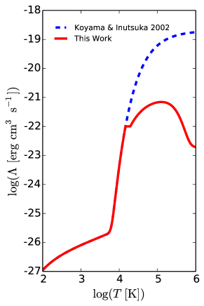
Figure 1: Comparison between the cooling functions from Koyama & Inutsuka (2002) (blue dashed) and from this work (red solid). Our modifications on Koyama & Inutsuka (2002) are motivated to calculate the cooling rate in the high-temperature regime, especially reflecting the facts that the thermal ionization of neutral hydrogen ($T\gtrsim 14,577$ K) and line emission by ionized carbon and oxygen (peaks at $T\sim 10^{5}$ K) (Cox & Tucker 1969; Dalgarno & McCray 1972).

We define the thermally unstable neutral medium (UNM) as $(\partial(\mathcal{L}/T)/\partial T)_{P}<0$ (e.g., Balbus 1986, 1995), and the gas state warmer (colder) than the UNM is classified as the WNM (CNM). We will use this definition hereafter when we analyze the mass fraction of each phase. Although the boundary between WNM, UNM, and CNM depends on both the density and temperature, the three phases roughly correspond to the WNM as $T\geq 5000$ K, the UNM as $100\leq T<5000$ K, and the CNM as $T<100$ K based on Equation 4.

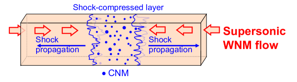
Figure 2: Schematic figure of our converging flow simulations. Supersonic WNM flows are continuously injected at the $x$ boundaries and flow inwards (red arrows). The shock-compressed layer forms at the center of the simulation box, sandwiched by two shock fronts (blue solid lines). It becomes thicken while the flow continues (blue arrows). Dense clumps whose density correspond to CNM form in the layer (blue points).

2.2 Setups and Shock Capturing

Table 1: Studied Parameters

Runs	Parameters
	Adiabatic (A)	Resolution	$\Delta\rho_{0}$	Phase	$\gamma$	Figures
	or Heating	$\Delta x$	$=\sqrt{\langle\delta\rho_{0}^{2}\rangle}/\rho_{0}$	$\alpha$
	& Cooling (C)	$($ pc $)$	$($ % $)$
	or Effective index (E)
A2D0000	A	0.02	0	N/A	$\gamma_{0}=$ 1.67	4
C2D0000	C	0.02	0	N/A	$\gamma_{0}=$ 1.67	4, and  2.3
C2D1000	C	0.02	100	$\alpha_{1}$, $\alpha_{2}$, $\alpha_{3}$	$\gamma_{0}=$ 1.67	2.3,  3.2,  2.2,  2.2,  10,  2.2,  2.2
C8D0316	C	0.08	31.6	$\alpha_{1}$, $\alpha_{2}$, $\alpha_{3}$	$\gamma_{0}=$ 1.67	3.2,  3.2,  3.2
C4D0316	C	0.04	31.6	$\alpha_{1}$, $\alpha_{2}$, $\alpha_{3}$	$\gamma_{0}=$ 1.67	3.2,  3.2,  3.2
C2D0316	C	0.02	31.6	$\alpha_{1}$, $\alpha_{2}$, $\alpha_{3}$	$\gamma_{0}=$ 1.67	2.3,  4,  3.2,  3.2,  3.2,  2.2,  10,  2.2,  2.2
C1D0316	C	0.01	31.6	$\alpha_{1}$	$\gamma_{0}=$ 1.67	3.2,  3.2, 3.2
C8D0100	C	0.08	10	$\alpha_{1}$, $\alpha_{2}$, $\alpha_{3}$	$\gamma_{0}=$ 1.67	3.2
C4D0100	C	0.04	10	$\alpha_{1}$, $\alpha_{2}$, $\alpha_{3}$	$\gamma_{0}=$ 1.67	3.2
C2D0100	C	0.02	10	$\alpha_{1}$, $\alpha_{2}$, $\alpha_{3}$	$\gamma_{0}=$ 1.67	2.3,  3.2,  2.2,  10,  2.2,  2.2
C1D0100	C	0.01	10	$\alpha_{1}$	$\gamma_{0}=$ 1.67	3.2
C8D0031	C	0.08	3.16	$\alpha_{1}$, $\alpha_{2}$, $\alpha_{3}$	$\gamma_{0}=$ 1.67	3.2,  3.2,  3.2
C4D0031	C	0.04	3.16	$\alpha_{1}$, $\alpha_{2}$, $\alpha_{3}$	$\gamma_{0}=$ 1.67	3.2,  3.2,  3.2
C2D0031	C	0.02	3.16	$\alpha_{1}$, $\alpha_{2}$, $\alpha_{3}$	$\gamma_{0}=$ 1.67	2.3,  3.2,  3.2,  3.2,  2.2,  2.2
C1D0031	C	0.01	3.16	$\alpha_{1}$	$\gamma_{0}=$ 1.67	3.2,  3.2,  3.2
C2D0010	C	0.02	1	$\alpha_{1}$, $\alpha_{2}$, $\alpha_{3}$	$\gamma_{0}=$ 1.67	2.3,  3.2,  2.2,  2.2,  10,  2.2,  2.2
C2D0003	C	0.02	0.316	$\alpha_{1}$, $\alpha_{2}$, $\alpha_{3}$	$\gamma_{0}=$ 1.67	2.3,  2.2,  2.2
C2D0001	C	0.02	0.1	$\alpha_{1}$, $\alpha_{2}$, $\alpha_{3}$	$\gamma_{0}=$ 1.67	2.3,  3.2,  2.2,  2.2
E2D0000	E	0.02	0	N/A	$\gamma_{0}=$ 1.67
					& $\gamma_{\rm eff}=0.863$	2.2

Note. 45 cases (out of total 69 cases) that we will present in this article. Details of individual parameters are described in Section 2. The run names represent the following first three columns. Each column represents as follows; The first column indicates whether we calculate adiabatic fluid (indicated as “A”), or include heating and cooling processes based on Equation 4 (indicated as “C”), or using the effective index $\gamma_{\rm eff}$ (indicated as “E”). Resolution shows the spatial resolution. Phases $\alpha_{1}$, $\alpha_{2}$, and $\alpha_{3}$ represent three different random phases for initial density fluctuation ($\alpha_{k_{y},k_{z}}$ in Equation 6), where N/A represents no fluctuation (i.e., $\sqrt{\langle\delta\rho_{0}^{2}\rangle}=0.0$). $\gamma$ lists the original specific heat $\gamma_{0}$ and the effective index $\gamma_{\rm eff}$. Figures list the corresponding figure numbers.

Figure 2 shows a schematic view of our simulations. The shock-compressed layer forms at the box center sandwiched by two shock fronts, and becomes thicken while the flow continues as the two shocks propagate outwards. Our three-dimensional simulation box has its size of $L_{x,y,z}=20,10,10$ pc, which is a typical size of giant molecular clouds in the Milky Way galaxy. Here $x$ is defined as the flow direction. The left and right parts of the WNM have the velocity in the opposite direction with $\left|v_{x}\right|=20$ km s^-1, colliding at the box center. The relative velocity between these two flows is thus $40\,{\rm km\,s^{-1}}$ in this $20\,{\rm km\,s^{-1}}$ + $20\,{\rm km\,s^{-1}}$ collision. This velocity is likely even faster in galaxy mergers (e.g., $>100\,{\rm km\,s^{-1}}$), but by employing 20 km s^-1, we opt to focus on more common situations in galactic disks (e.g., the late phase of supernova remnants expansions, H ii region expansions, and normal shock due to galactic spirals). For the initial velocity field, we may simply flip the sign of the velocity at $x=L_{x}/2$. However, as a more conservative approach to avoid any artifacts that may arise from such a step-function collision, we apply $\tanh$ smoothing as

$$v_{x}=V_{\rm in}\tanh\left(\frac{x-L_{x}/2}{n_{\rm smx}\Delta x}\right)\,,$$ (5)

so that the initial collision occurs smoothly. Here $V_{\rm in}=20$ km s^-1 and $\Delta x$ is the mesh size. $n_{\rm smx}$ is chosen such that the physical scale of this smoothing is constant as $n_{\rm smx}\Delta x=0.78$ pc between different resolution runs.

The WNM is continuously injected through the two $x$ boundaries at $x=0$ and $20$ pc until the calculation ends at 3 Myr, whereas $y$ and $z$ boundaries have the periodic boundary condition. The WNM flow is in a thermally stable phase having the mean number density $n_{0}=0.57\,\mbox{${\rm cm^{-3}}$}$ and pressure $P_{0}/k_{\rm B}=3500\,\mathrm{K\,cm^{-3}}$. The corresponding mean temperature, sound speed, and dynamical pressure are $6141$ K, $C_{\rm s}=8.16\,{\rm km\,s^{-1}}$, and $2.6\times 10^{4}\,\mathrm{K\,cm^{-3}}$, respectively, where we use $\rho_{0}=n_{0}\mu_{\rm M}m_{\rm p}$ with $\mu_{\rm M}=1.27$ as the mean molecular weight (c.f., Inoue & Inutsuka 2008, 2012).

The mass density of the WNM flow has a fluctuation as $\rho(x,y,z)=\rho_{0}+\delta\rho_{0}(x,y,z)$:

$$\delta\rho_{0}(x,y,z) = \sum_{k_{x},k_{y},k_{z}}A(k)$$ (6)

$$\times\sin(k_{x}x+k_{y}y+k_{z}z+\alpha_{k_{x},k_{y},k_{z}})\,.$$

$k_{x}$, $k_{y}$ and $k_{z}$ are the wave numbers in $x$, $y$ and $z$-directions as $k_{x}=2\pi l_{x}/(L_{x}/2)$, $k_{y}=2\pi l_{y}/L_{y}$ and $k_{z}=2\pi l_{z}/L_{z}$ while the integers $l_{x}$, $l_{y}$ and $l_{z}$ span from $-32$ to $32$. $A(k)$ is set such that the density power spectrum follows the Kolmogorov spectrum $P_{\rho}(k)\propto k^{-11/3}$ where $k=\sqrt{k_{x}^{2}+k_{y}^{2}+k_{z}^{2}}$ (Kolmogorov 1941; Armstrong et al. 1995). As indicated in the definition of $k_{x}$, we generate this fluctuation over a 10 pc $\times$ 10pc $\times$ 10pc volume so that the initial left-half ($x=0$ – $10$ pc) and right-half ($x=10$ – $20$ pc) of the WNM have the same density distribution (so as the temperature distribution does to achieve the initial pressure equilibrium). The WNM flow injected from the boundaries also follow this density distribution as the flows move inward, and the WNM accrete onto the shock-compressed layer always with this density fluctuation.

To identify the shock-compressed layer, we search cells along $x$ direction at every given $(y,z)$ inward from both $x$ boundaries, and label the first cells with $P>1.3P_{0}$. We calculate the arithmetic mean of the distances from the box-center to these positions as the representative shock front position:

$$\langle x_{\rm shock}\rangle=\frac{\sum_{y,z}\left(x_{\rm R}(y,z)-x_{\rm L}(y,z)\right)}{2N_{yz}}\,,$$ (7)

where the subscripts $\mathrm{R}$ and $\mathrm{L}$ denote the two shock front positions (the right and left side of the layer), and $N_{yz}$ denotes the total number of cells on $y$-$z$ plane. The factor of 2 in the denominator means that there are two shocks and the overall mean position of the shock front is the half of $x_{\rm R}-x_{\rm L}$ at every given $(y,z)$. We then measure the mean density within the shock-compressed layer $\langle n\rangle$ accordingly, as the gas density averaged over the entire volume of the shock-compressed layer defined above.

2.3 Range of Systematic Study

As a systematic study, we opt to vary two properties: the amplitude of the density fluctuation $\langle A\rangle$ and the spatial resolution $\Delta x$. We vary $\langle A\rangle$ such that the mean dispersion of the density $\Delta\rho_{0}=\sqrt{\langle\delta\rho_{0}^{2}\rangle}/\rho_{0}$ spans as $100$, $31.6$, $10$, $3.16$, $1$, $0.361$, $0.1$ %. This $100$ % is motivated by the fact that density inhomogeneity exists on all spatial scales in the diffuse ISM (e.g., Armstrong et al. 1995; Lazarian & Pogosyan 2000; Chepurnov & Lazarian 2010), and the column density of Hi gas likely varies with the order of unity (e.g., Burkhart et al. 2015; Fukui et al. 2018). We also investigate the conditions with extremely low levels of fluctuation (as low as $0.1$ %) to understand the dependence of $\Delta\rho_{0}$. We choose the spatial resolution of $\Delta x=$ $7.8\times 10^{-2}$, $3.9\times 10^{-2}$, $2.0\times 10^{-2}$ and $9.8\times 10^{-3}$ pc by splitting the calculation domain with from 256 $\times$ 256 $\times$ 128 cells at the lowest resolution up to 2048 $\times$ 1024 $\times$ 1024 cells at the highest resolution (hereafter noted as $\Delta x=0.08$ pc, $0.04$ pc, $0.02$ pc, and $0.01$ pc for simplicity in the text and figures). In addition, we repeat simulations with the same $\Delta\rho_{0}$ and $\Delta x$ but with three different random phases $\alpha_{1}$, $\alpha_{2}$, and $\alpha_{3}$ to investigate the possible range over which the averaged properties vary due to such randomness even under the same statistical condition. Note that the highest resolution is computationally expensive and is limited to study in 3 representative cases only ($\Delta\rho_{0}=31.6$, $10$, and $3.16$ % with Phase $\alpha_{1}$).

(a) $\Delta\rho_{0}=$ 100%                                                      (d) $\Delta\rho_{0}=$ 3.16%

Figure 3: The density slice on $z=5$ pc plane at $1.8$ Myr, where the color represents $\log(n[{\rm cm^{-3}}])$. The horizontal and vertical axes are $x$ and $y$ directions in the unit of pc. The thin black lines show the shock front positions. The panels correspond to (a) $\Delta\rho_{0}=$ 100% (Run C2D1000), (b) 31.6% (Run C2D0316), (c) 10% (Run C2D0100), (d) 3.16% (Run C2D0031), (e) 1% (Run C2D0010), and (f) 0 % (Run C2D0000) with Phase $\alpha_{1}$. Note that small-scale details are smeared out on these figures due to rasterization.

(b) $\Delta\rho_{0}=$ 31.6%                                                      (e) $\Delta\rho_{0}=$ 1%                 (c) $\Delta\rho_{0}=$ 10%                                                         (f) $\Delta\rho_{0}=$ 0%      

The combination of these 3(+1) resolutions, 7 fluctuation amplitudes, and 3 phases corresponds to 66 cases. We additionally perform 3 controlled runs as a reference, where we investigate head-on collisions with the upstream WNM density completely uniform ($\Delta\rho_{0}=0$ %). We thus investigate 69 cases in total. Table 2.2 summarizes the parameter sets, where we list 45 cases that we will present in this article, out of the total 69 cases. The calculation results are sampled every 0.1 Myr in each run.

3 Results

3.1 General Outcomes

In this section, we provide a brief overview of our simulation results, showing how the geometrical structure of the shock-compressed layer varies with $\Delta\rho_{0}$ and cooling process. Figure 2.3 shows the gallery of the density slice from runs with $\Delta\rho_{0}=$ 100% (Run C2D1000), 31.6% (Run C2D0316), 10% (Run C2D0100), 3.16% (Run C2D0031), 1% (Run C2D0010), and 0 % (Run C2D0000) with Phase $\alpha_{1}$ and $\Delta x=0.02$ pc. The shock-compressed layer is wider and wound more significantly with larger $\Delta\rho_{0}$ due to the larger density fluctuation, whereas the layer is narrower and tends to be less deformed with smaller $\Delta\rho_{0}$. Non-zero $\Delta\rho_{0}$ provides the interaction between shocks and density inhomogeneity, which drives turbulence in the shock-compressed layer. In contrast, $\Delta\rho_{0}=0$ % is an extreme condition where the flow becomes one-dimensional (i.e., the layer maintains a completely straight geometry), and all the mass of the WNM flow cools down and eventually accretes onto the thin CNM sheet formed at the center.

Figure 4 shows the time evolution of $\langle x_{\rm shock}\rangle$ from three runs: an adiabatic flow with $\Delta\rho_{0}=0$ % (Run A2D0000, “1D adiabatic”), a flow with cooling with $\Delta\rho_{0}=0$ % (Run C2D0000, “1D with cooling”), and a flow with cooling with $\Delta\rho_{0}=31.6$ % with Phase $\alpha_{1}$ (Run C2D0316, “3D with cooling”). As seen from the difference between Runs A2D0000 and C2D0000, the cooling process transforms the WNM to the CNM and the shock-compressed layer becomes denser and narrower. As shown in Run C2D0316, a non-zero $\Delta\rho_{0}$ converts a fraction of the WNM to the CNM and drive some turbulence, which makes the shock-compressed layer less dense and wider compared with the uniform case (Run C2D0000), but still significantly denser and narrower than the adiabatic case (Run A2D0000). All the shock-compressed layer with non-zero $\Delta\rho_{0}$ in our simulations evolves somewhere between Runs A2D0000 and C2D0000, accordingly.

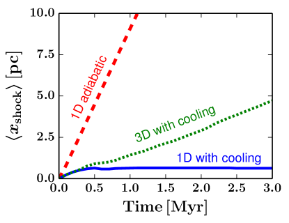
Figure 4: The time evolution of $\langle x_{\rm shock}\rangle$ from three runs: an adiabatic flow with $\Delta\rho_{0}=0$ % (Run A2D0000, red dasehd line “1D adiabatic”), a flow with cooling with $\Delta\rho_{0}=0$ % (Run C2D0000, blue solid line “1D with cooling”), and a flow with cooling with $\Delta\rho_{0}=31.6$ % with Phase $\alpha_{1}$ (Run C2D0316, green dotted line “3D with cooling”).

3.2 Convergence with Respect to the Spatial Resolution

(a) $\Delta\rho_{0}=$ 31.6%                                                      (b) $\Delta\rho_{0}=$ 3.16%

Figure 5: Panels (a) and (b): The mass histogram on the $P$-$n$ diagram at 3 Myr, where $\Delta\rho_{0}=31.6$ % (Run C2D0316, Panel (a)) and $3.16$ % (Run C2D0031, Panel (b)), both of which employ Phase $\alpha_{1}$ and $\Delta x=0.02$ pc. The blue color corresponds to $\log($mass$[\mbox{${\rm M_{\odot}}$}])$. The red solid curve shows the thermal equilibrium region where the heating and cooling balances each other defined as $\rho\mathcal{L}=0$. The horizontal black dashed line shows the ram pressure of the flow $\rho_{0}V_{\rm in}^{2}$. The thin black curve encloses the region of the UNM defined as $(\partial(\mathcal{L}/T)/\partial T)_{P}<0$. The horizontal and vertical axes are logarithmically equally binned by a factor $1.26$. Panels (c) and (d): The histogram of the effective cooling length $\lambda_{\rm cool,eff}$ in the shock-compressed layer at 3 Myr, where again $\Delta\rho_{0}=31.6$ % (Run C2D0316, Panel (c)) and $3.16$ % (Run C2D0031, Panel (d)). The blue curve shows the CNM, the green for the UNM, and red for the WNM, whereas the black curve shows the total of these components. The horizontal axis is logarithmically equally binned by a factor $1.26$.

(c) $\Delta\rho_{0}=$ 31.6%                                                      (d) $\Delta\rho_{0}=$ 3.16%      

(a) $\Delta\rho_{0}=$ 31.6 %                                                      (b) $\Delta\rho_{0}=$ 3.16 %

Figure 6: Panels (a) and (b): The time evolution of the average shock front position $\langle x_{\rm shock}\rangle$ as a function of the spatial resolution $\Delta x$, where $\Delta\rho_{0}=31.6$ % (Runs C*D0316, Panel (a)) and $3.16$ % (Runs C*D0031, Panel (b)), both of which employ Phase $\alpha_{1}$. The color corresponds to the spatial resolution. Panels (c) and (d): Same as Panels (a) and (b) but shows the time evolution of the mean density $\langle n\rangle$.

(c) $\Delta\rho_{0}=$ 31.6%                                                      (d) $\Delta\rho_{0}=$ 3.16%      

(a) $\Delta\rho_{0}=$ 31.6%                                                      (b) $\Delta\rho_{0}=$ 3.16%

Figure 7: Panels (a) and (b): The mass frequency ${\rm d}M/{\rm d}\log(n)$ as a function of $n$ at 3 Myr with $\Delta\rho_{0}=31.6$ % (Runs C*D0316, Panel (a)) and $3.16$ % (Runs C*D0031, Panel (b)), both of which employ Phase $\alpha_{1}$. The color corresponds to the spatial resolution $\Delta x$. The vertical lines show the mean density $\langle n\rangle$, whose color coding is matched with each spatial resolution. Panel (c): Compilation of the mass frequency from $\Delta\rho_{0}=$ 100% (Run C2D1000), 31.6% (Run C2D0316), 10% (Run C2D0100), 1% (Run C2D0010), and 0.1 % (Run C2D0001). The shades in each $\Delta\rho_{0}$ show the range of the maximum and minimum due to Phases $\alpha_{1}$, $\alpha_{2}$, and $\alpha_{3}$. Note that the shades of $\Delta\rho_{0}=1$ % and $0.1$ % are difficult to read because they are almost overlapped. Panel (d): the ratio of $\langle n\rangle(\Delta x,\alpha)$ to the $\langle n\rangle(0.01\,\mathrm{pc},\alpha_{1})$ in each $\Delta\rho_{0}$. The grey shades correspond to the range of the maximum and minimum due to Phases $\alpha_{1}$, $\alpha_{2}$, and $\alpha_{3}$. The colored points correspond to the average within each combination of ($\Delta\rho_{0}$, $\Delta x$), where the colors correspond to $\Delta x=0.08$ pc (red), $0.04$ pc (orange), and $0.02$ pc (green). Note that runs with $\Delta x=0.01$ pc are limited to Phase $\alpha_{1}$, and therfore the denominator in the vertical axis is a single value $\langle n\rangle$ from the Phase $\alpha_{1}$ but not the average of the three phases.

(c) Various $\Delta\rho_{0}$ with $\Delta x=0.02$ pc                                     (d) Variation with respect to $\Delta x=0.01$ pc      

We first investigate the convergence with respect to the spatial resolution $\Delta x$ by varying it from $0.08$ pc to $0.01$ pc in all $\Delta\rho_{0}$ cases as shown in Table 2.2. We find that the mean properties of the shock-compressed layer is converged with $0.02$ pc spatial resolution in any $\Delta\rho_{0}$ case, but the trend of convergence differs between the cases with larger $\Delta\rho_{0}>10$ % and with smaller $\Delta\rho_{0}\leq 10$ %. Therefore in this section, we show the results mainly from $\Delta\rho_{0}=31.6$ % and $3.16$ % as examples of large and small $\Delta\rho_{0}$ and investigate how the physical properties of the shock-compressed layer converge.

Panels (a) and (b) in Figure 3.2 show the mass histogram on the $P$-$n$ diagram at 3 Myr from $\Delta\rho_{0}=31.6$ % (Run C2D0316, Panel (a)) and $3.16$ % (Run C2D0031, Panel (b)). Most mass resides in two regions: the shock-heated component (WNM and UNM at $n\simeq 2\mbox{${\rm cm^{-3}}$}$) and the cooled component (CNM at $n>100\mbox{${\rm cm^{-3}}$}$). As shown here, the WNM density is typically 100 times diffuse than that of CNM, and the volume of the shock-compressed layer is dominated by the WNM. Therefore, resolving the typical transition scale from the WNM into CNM is crucial for the convergence in the mean properties of the shock-compressed layer, while resolving the CNM cooling length is important when we investigate the detailed structures of CNM clumps. We thus investigate the effective cooling length $\lambda_{\rm cool,eff}$ in the shock-compressed layer at 3 Myr. Panels (c) and (d) in Figure 3.2 show its histogram. Here we calculate $\lambda_{\rm cool,eff}$ as $C_{\rm s}P/(\gamma-1)/(n^{2}\Lambda-n\Gamma+P\nabla_{\mu}v_{\mu})$ in each cell where $C_{\rm s}$ and $P$ are the sound speed and thermal pressure in each cell. The panels show that $0.02$ pc corresponds to the typical spatial scale on which the dominant components in the cooling length transits from the UNM to CNM. We also find that the spatial resolution of $0.02$ pc fully resolves the WNM cooling length, and resolves the cooling length of more than 99 % (92 %) of the UNM in volume (mass) when $\Delta\rho_{0}=31.6$ % and more than 98 % (80 %) when $\Delta\rho_{0}=3.16$ %. We thus expect that the mean properties converge when $\Delta x=0.02{\rm~{}pc}$ or higher resolution, with which we can follow the dynamical condensation from WNM and UNM to CNM due to cooling.

This characteristic scale of $0.02$ pc is also consistent with the resolution requirement empirically suggested by previous numerical simulations. For example, Inoue & Omukai (2015) performed converging flow calculations similar to our studies, and suggested that more than 60 cells on the most frequent cooling length (defined as $\lambda_{\rm cool}=C_{\rm s}P/(\gamma-1)/(n^{2}\Lambda)$) is required to have convergence in the mass probability distribution function and CNM clump mass function. In our simulations, the mean cooling scale $\langle\lambda_{\rm cool}\rangle$ is peaked at the WNM and UNM component with $3.4$ pc in $\Delta\rho_{0}=31.6$ % and $2.2$ pc in $3.16$ %. The requirement of more than 60 cells over one cooling scale corresponds to $\Delta x<0.037$ pc, accordingly.

Panels (a) – (d) in Figure 3.2 show such convergence in the mean properties; the time evolution of $\langle x_{\rm shock}\rangle$ and $\langle n\rangle$ as a function of $\Delta x$ with Phase $\alpha_{1}$, where Panels (a) and (c) for $\Delta\rho_{0}=31.6$ % and (b) and (d) for $3.16$ %. In both $\Delta\rho_{0}$ cases, the linear growth of $\langle x_{\rm shock}\rangle$ (i.e., the constant speed of the shock propagation) corresponds to the quasi-steady $\langle n\rangle$. As already seen in Figure 2.3, the larger (smaller) $\Delta\rho_{0}$ results in a wider (narrower) layer and smaller (denser) $\langle n\rangle$. The measured $\langle x_{\rm shock}\rangle$ and $\langle n\rangle$ at 3 Myr are listed on Table 3.2. These results suggest that $\langle x_{\rm shock}\rangle$ and $\langle n\rangle$ indeed show a convergence with $\Delta x=0.02$ pc, with less than 17 % difference between the results of $\Delta x=0.02$ pc and $0.01$ pc.

The trend of convergence, however, differs between large and small $\Delta\rho_{0}$. For example, $\langle x_{\rm shock}\rangle$ and $\langle n\rangle$ of Runs C*D0316 do not vary monotonically along with $\Delta x$ whereas those of Runs C*D0031 do. In addition, the difference in $\langle x_{\rm shock}\rangle$ and $\langle n\rangle$ at 3 Myr between $\Delta x=0.08$ pc and $0.01$ pc is limited to a factor of $0.11$ in Runs C*D0316 but is by a factor of $2.09$ in Runs C*D0031. Thus overall, convergence with large $\Delta\rho_{0}$ is non-monotonic and calculations with coarse resolutions of $\geq 0.02$ pc show similar values in $\langle x_{\rm shock}\rangle$ and $\langle n\rangle$, whereas the convergence with small $\Delta\rho_{0}$ is monotonic and stringently requires $0.02$ pc as expected from the cooling length analysis above.

To understand these trends, we investigate the mass frequency as a function of density within the shock-compressed layer, which is shown in Panels (a) and (b) of Figure 3.2 with $\langle n\rangle$ as vertical lines. We also measure the mass fraction of WNM ($f_{\rm WNM}$), UNM ($f_{\rm UNM}$), and CNM ($f_{\rm CNM}$), and the peak density of the CNM $n_{\rm CNM\,peak}$, which are summarized on Table 3.2. The bimodality commonly appears in both $\Delta\rho_{0}$ cases, which shows the shock-heated component peaked at $n\sim 2$ – $4\,\mbox{${\rm cm^{-3}}$}$ mostly corresponding to the WNM and UNM, and the cooled component peaked at $n\sim 100$ – $400\,\mbox{${\rm cm^{-3}}$}$ mostly corresponding to the CNM. The relative mass fraction, however, depends on $\Delta\rho_{0}$. $f_{\rm CNM}$ remains $\sim 45$ % when $\Delta\rho_{0}=31.6$ % and both the WNM+UNM and CNM contribute to $\langle n\rangle$, whereas $f_{\rm CNM}$ is $\sim 70$ % when $\Delta\rho_{0}=3.16$ % and $\langle n\rangle$ depends more on the CNM component. For example, $\langle n\rangle$ with $\Delta\rho_{0}=31.6$ % shifts non-monotonically in accordance with the non-monotonic change in the WNM fraction with $\Delta x$, resulting in similar $\langle n\rangle$ between different $\Delta x$. In contrast, $\langle n\rangle$ with $\Delta\rho_{0}=3.16$ % shifts monotonically by the factor as $n_{\rm CNM,peak}$ monotonically shifts with $\Delta x$ (e.g., from $\Delta x=0.08$ pc to $0.01$ pc, $\langle n\rangle$ shifts from $12.0$ to $24.7\,\mbox{${\rm cm^{-3}}$}$ with $n_{\rm CNM,peak}$ from $200$ to $400\,\mbox{${\rm cm^{-3}}$}$).

Table 2: Physical properties at 3 Myr from $\Delta\rho_{0}=31.6$ % (Runs C*D0316) and $3.16$ % (Runs C*D0031) with Phase $\alpha_{1}$, with respect to the spatial resolution $\Delta x$.

Two distinct behaviors depending on $\Delta\rho_{0}$ appear also with different random phases $\alpha_{1}$, $\alpha_{2}$, and $\alpha_{3}$ in the upstream density fluctuation. Panel (c) of Figure 3.2 shows the mass frequency variation due to those three random phases in each $\Delta\rho_{0}$ under a fixed power spectrum of $P_{\rho}(k)\propto k^{-11/3}$ and a fixed spatial resolution of $\Delta x=0.02$ pc. This shows that the mass frequency has a larger variation by the random phases $\alpha$ in larger $\Delta\rho_{0}$ cases. To compare this variation due to different $\alpha$ with the variation due to $\Delta x$, Panel (d) of Figure 3.2 shows the ratio of $\langle n\rangle(\Delta x,\alpha)$ to the $\langle n\rangle(0.01\,\mathrm{pc},\alpha_{1})$ in each $\Delta\rho_{0}$. In the case of $\Delta\rho_{0}=31.6$ %, we found that the variation due to different $\alpha$ and that due to different $\Delta x$ are comparable (i.e., the width of grey shades is comparable to the scatter of points around the unity). This suggests that resolving the density fluctuation with different $\Delta x$ also intrinsically produces the variation in $\langle n\rangle$ comparable to the variation produced by different $\alpha$. Therfore, $\langle n\rangle$ converges non-monotonically and calculations with coarse resolutions of $\Delta x>0.02$ pc practically provide simliar values in $\langle x_{\rm shock}\rangle$ and $\langle n\rangle$ even though the physical convergence still requires $\Delta x=0.02$ pc. The physical origin of such variation due to different $\Delta x$ is explained by the non-linear nature of the system, which we will discuss in Section 4.2. In contrast in the case of $\Delta\rho_{0}\leq 10$ %, we found that the variation due to different $\alpha$ is limited, and the effect of changing $\Delta x$ directly appears as a monotonic change of $\langle n\rangle$, showing the convergence as predicted by the cooling length analysis.

Therefore in the following sections, we will focus on the results based on $\Delta x=0.02$ pc and highlight how the physical properties of the shock-compressed layer varies with $\Delta\rho_{0}$ and the random phases.

Figure 8: Left: The time evolution of the average shock front position $\langle x_{\rm shock}\rangle$ as a function of $\Delta\rho_{0}$ with $\Delta x=0.02$ pc. The color corresponds to $\Delta\rho_{0}$. The shades in each $\Delta\rho_{0}$ show the range of the maximum and minimum due to Phase $\alpha_{1}$, $\alpha_{2}$, and $\alpha_{3}$. Right: the dispersion of the shock front position $\sqrt{\langle\delta x_{\rm shock}^{2}\rangle}$ as a function of $\Delta\rho_{0}$ at 1, 2, and 3 Myr. We here average the results of three random phases at each time step.

(a) $\Delta\rho_{0}=$ 100%                                                      (b) $\Delta\rho_{0}=$ 1%

Figure 9: Panels (a) and (b): $v_{x}[{\rm{\rm km\,s^{-1}}}]$ slice on $z=5$ pc plane at $1.8$ Myr, where $\Delta\rho_{0}=31.6$ % (Run C2D0316, Panel (a)) and $3.16$ % (Run C2D0031, Panel (b)), both of which employ Phase $\alpha_{1}$ and $\Delta x=0.02$ pc. Panels (c) and (d): Same as Panels (a) and (b) but the $y$-component of vorticity, $\log\left(\left|(\nabla\times\mathbf{v})_{\rm y}\right|[{\rm s^{-1}}]\right)$.

(c) $\Delta\rho_{0}=$ 100%                                                      (d) $\Delta\rho_{0}=$ 1%      

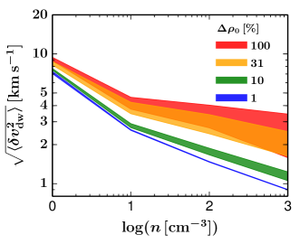
Figure 10: The density-weighted velocity dispersion $\sqrt{\langle\delta v_{\rm dw}^{2}\rangle}$ as a function of $n$ and $\Delta\rho_{0}$ with $\Delta x=0.02$ pc. The color corresponds to $\Delta\rho_{0}$ and the shades show the range of the maximum and minimum due to Phase $\alpha_{1}$, $\alpha_{2}$, and $\alpha_{3}$ in each $\Delta\rho_{0}$. Note that the vertical axis is also in the logarithmic scale. Also note that the horizontal axis has logarithmically equal bins as $\log(n[\mbox{${\rm cm^{-3}}$}])=[0,1),[1,2),[2,3),[3,\infty)$ and each bin is plotted at their lower limit density.

Figure 11: Left: the density-weighted velocity dispersion $\sqrt{\langle\delta v_{\rm dw}^{2}\rangle_{\rm tot}}$ as a function of $\Delta\rho_{0}$ at 1, 2, and 3 Myr. The subscription “tot” means that we take the average over the entire volume of the shock-compressed layer and we take the average of three random phases at each time step. Right: the energy conversion rate from the upstream kinetic energy into the post-shock turbulence energy ($\epsilon_{\rm turb}$, blue), and into the post-shock thermal energy ($\epsilon_{\rm th}$, red) as a function of $\Delta\rho_{0}$ at 1 and 3 Myr.

3.3 Geometry and Turbulence

We found that two distinct behaviors depending on $\Delta\rho_{0}$ appear also on the geometry of the shock-compressed layer corresponding to large/small $\Delta\rho_{0}$. The left panel of Figure 2.2 summarizes the time evolution of the average shock front position $\langle x_{\rm shock}\rangle$ for each $\Delta\rho_{0}$ with $\Delta x=0.02$ pc. The shades in each $\Delta\rho_{0}$ show the range of the maximum and minimum due to the three random phases $\alpha$. This shows that the shock-compressed layer becomes wider (with larger variation by different $\alpha$) when $\Delta\rho_{0}$ is larger, which one can visually confirm also in the density snapshots already shown in Figure 2.3. In addition, we investigate the dispersion of $\langle x_{\rm shock}\rangle$, defined as

$$\sqrt{\langle\delta x_{\rm shock}^{2}\rangle}=\frac{\sum_{y,z}\sqrt{(x_{\rm R}(y,z)-\bar{x}_{\rm R})^{2}+(x_{\rm L}(y,z)-\bar{x}_{\rm L})^{2}}}{2N_{yz}}\,,$$ (8)

where $\bar{x}_{\rm R}$ and $\bar{x}_{\rm L}$ are the mean position of the right and left shocks, respectively, and the results are summarized in the right panel of Figure 2.2. $\sqrt{\langle\delta x_{\rm shock}^{2}\rangle}$ gradually grows in time in all $\Delta\rho_{0}$ cases, especially density inhomogeneity with larger $\Delta\rho_{0}$ deforms shock fronts more significantly whose amplitude reaches a fraction of 10 pc (the size of the cross section of the computational domain). Given that the Kolmogorov spectrum in the upstream density fluctuation has a larger power on larger scales (Equation 6), we expect that the shock deformation is apparent on larger scales. The shock front geometry of $\Delta\rho_{0}=100$ %, for example, indeed indicates the impact from the largest-scale mode of $\lvert k\rvert=2\pi/L_{y}$ (e.g., Panel (a) of Figure 2.3). Smaller $\Delta\rho_{0}$ introduces less deformation and the shock front geometry becomes closer to the completely straight front observed in $\Delta\rho_{0}=0$ % (e.g., Panels (d) and (e) of Figure 2.3).

The two modes in these geometries, combined with the WNM:CNM mass fraction in Section 3.2, suggest that large-scale oblique shocks induced by significant shock deformation with larger $\Delta\rho_{0}$ suppresses the energy dissipation at the shock fronts, driving stronger turbulence and forming less CNM in the shock-compressed layer, and vice versa for smaller $\Delta\rho_{0}$ cases. We thus investigate the velocity and vorticity structure of the shock-compressed layer and the results are shown in Figure 2.2. We here choose $\Delta\rho_{0}=100$ % and $1$ % to clearly highlight the difference between large and small $\Delta\rho_{0}$. There are indeed fast WNM flows that continue into the shock-compressed layer without significant vorticity generation when $\Delta\rho_{0}$ is large (e.g., $3$ pc $\lesssim y\lesssim 7$ pc in Panels (a) and (c)), whereas most of the flow is well decelerated when $\Delta\rho_{0}$ is small (in Panels (b) and (d)). We also measure the density-weighted velocity dispersion $\sqrt{\langle\delta v_{\rm dw}^{2}\rangle}$ as a function of $n$ and $\Delta\rho_{0}$, which is shown in Figure 10. The bimodal behavior depending on $\Delta\rho_{0}$ appears also in this $\sqrt{\langle\delta v_{\rm dw}^{2}\rangle}$ as we expected; the less-decelerated fast flow of the WNM in larger $\Delta\rho_{0}$ cases drive larger $\sqrt{\langle\delta v_{\rm dw}^{2}\rangle}$ with significant variation due to different $\alpha$.

Note that the high-density structures predominantly contribute to the turbulent energy density $\rho\langle\delta v_{\rm dw}^{2}\rangle$ in any $\Delta\rho_{0}$ cases because the overall $n$-dependence of $\sqrt{\langle\delta v_{\rm dw}^{2}\rangle}$ is $\sqrt{\langle\delta v_{\rm dw}^{2}\rangle}\propto n^{-m}$ with $m\leq 0.5$ in the range of $n=1$ – $1000\,\mbox{${\rm cm^{-3}}$}$. In addition, $\sqrt{\langle\delta v_{\rm dw}^{2}\rangle}$ is dominated by the $x$-component because the converging-flow has a directionality in $x$. We found that the $x$-component of $\sqrt{\langle\delta v_{\rm dw}^{2}\rangle}$ amounts to $>70$ % of the total $\sqrt{\langle\delta v_{\rm dw}^{2}\rangle}$ in all density range in any $\Delta\rho_{0}$ cases. Such anisotropic turbulence is reported even in magnetized converging flow simulations when the magnetic fields are mostly parallel to the gas flow (e.g., Vázquez-Semadeni et al. 2007; Inoue & Inutsuka 2012; Iwasaki et al. 2019).

Also note that the overall decreasing trend of $\sqrt{\langle\delta v_{\rm dw}^{2}\rangle}$ with $n$ is consistent with other simulations and observations. For example, the velocity dispersion $\geq 2\,{\rm km\,s^{-1}}$ at $n<1\,\mbox{${\rm cm^{-3}}$}$ is reported from recent observations of the WNM absorption feature (e.g., Patra et al. 2018). The velocity dispersion $\leq 2\,{\rm km\,s^{-1}}$ at $n>10\,\mbox{${\rm cm^{-3}}$}$ is reported in previous converging WNM flow studies without magnetic fields (e.g., Heitsch et al. 2006). Fukui et al. (2018) also report this decreasing trend of $\sqrt{\langle\delta v_{\rm dw}^{2}\rangle}$ with $n$, where they perform synthetic observations of Hi line profiles in magnetohydrodynamics simulations and compare with emission-absorption measurements along quasar line of sights.

3.4 Energy Partition

Finally, we investigate the energy partition in the shock-compressed layer and its dependence on $\Delta\rho_{0}$. The left panel of Figure 2.2 shows the time evolution of $\sqrt{\langle\delta v_{\rm dw}^{2}\rangle_{\rm tot}}$ as a function of $\Delta\rho_{0}$. The subscription “tot” means that we take the average both over the entire volume of the shock-compressed layer and over the three random phases. This again clearly shows the bimodal behavior with respect to $\Delta\rho_{0}$, as expected from Figure 10. In addition, we found that small $\Delta\rho_{0}\leq 10$ % creates the velocity dispersion of $2.0$ – $3.2\,{\rm km\,s^{-1}}$ even down to $\Delta\rho_{0}=0.1$ %. The value of $\sim 2\,{\rm km\,s^{-1}}$ is consistent with the dispersion driven by the thermal instability alone (e.g., Koyama & Inutsuka 2002, 2006). This result indicates that shocks are always able to drive the velocity dispersion of $\sim 2\,{\rm km\,s^{-1}}$ through the thermal instability even when they propagate though the ISM with an almost uniform density.

Based on this $\sqrt{\langle\delta v_{\rm dw}^{2}\rangle_{\rm tot}}$, we measure the conversion rate of the upstream kinetic energy into the post-shock turbulent and thermal energy as

$$\epsilon_{\rm turb}(t)=\frac{M_{\rm total}(t)\,\langle\delta v_{\rm dw}^{2}(t)\rangle_{\rm tot}/2}{\int\dot{M}_{\rm total}(t)\,V_{\rm in}^{2}/2\,{\rm d}t}=\frac{\langle\delta v_{\rm dw}^{2}(t)\rangle_{\rm tot}}{V_{\rm in}^{2}}\,,$$ (9)

$$\epsilon_{\rm th}(t)=\frac{\int P(\mathbf{x},t){\rm d}\mathbf{x}/(\gamma-1)}{\int\dot{M}_{\rm total}(t)\,V_{\rm in}^{2}/2\,{\rm d}t}=\frac{\langle P(t)\rangle_{\rm tot}/(\gamma-1)}{\langle\rho(t)\rangle_{\rm tot}V_{\rm in}^{2}/2}\,.$$ (10)

Here $\dot{M}_{\rm total}(t)$ denotes the mass accretion rate into the shock-compressed layer at time $t$, which can be approximated as $\dot{M}_{\rm total}(t)\simeq 2\rho_{0}L_{y}L_{z}(V_{\rm in}+V_{\rm shock}(t))$. Note that $V_{\rm in}=20\,{\rm km\,s^{-1}}={\rm Const.}$ and we can assume $V_{\rm shock}={\rm Const.}$ as a zeroth-order estimation based on the time-evolution of $\langle x_{\rm shock}\rangle$. Therefore, we use $M_{\rm total}(t)=\int\dot{M}_{\rm total}(t){\rm d}t$ to obtain the second equality both in Equations 9 and 10.

The right panel of Figure 2.2 shows $\epsilon_{\rm turb}$ and $\epsilon_{\rm th}$ as a function of $\Delta\rho_{0}$ and time. The bimodal behavior depending on $\Delta\rho_{0}$ again appears in $\epsilon_{\rm turb}$ and $\epsilon_{\rm th}$ individually, and appears also in the relative importance of $\epsilon_{\rm turb}$ and $\epsilon_{\rm th}$; for example, at 3 Myr, the turbulent and thermal pressures equally support the shock-compressed layer when $\Delta\rho_{0}\leq 10$ % whereas the turbulence dominates when $\Delta\rho_{0}>10$ %.

In small $\Delta\rho_{0}$ cases, the shock-compressed layer is initially supported by the thermal pressure with limited turbulence. As CNM formation proceeds and the turbulence is developed (as seen in the left panel of Figure 2.2), the turbulent and thermal pressures start to equally support the shock-compressed layer. The sum of $\epsilon_{\rm turb}$ and $\epsilon_{\rm th}$ is limited to $<10$ % of the injected kinetic energy due to the radiation energy loss (implemented as the source term $\rho\mathcal{L}$ in Equation 3). In larger $\Delta\rho_{0}$ cases, strong turbulence prevents the dynamical condensation by cooling and the following CNM formation. The shock-compressed layer is occupied by the low-density high-temperature WNM and UNM (see the $P-n$ diagram of Figure 3.2), which keeps $\epsilon_{\rm th}$ higher than that in smaller $\Delta\rho_{0}$ cases. The turbulence dominantly supports the shock-compressed layer at 3 Myr and $\epsilon_{\rm turb}$ reaches $12.4$ % at maximum. Such a high conversion rate is consistent with the one driven by the interaction between shocks and density inhomogeneity (e.g., Inoue et al. 2012, 2013; Iwasaki et al. 2019). Inoue et al. 2013 showed that the growth velocity of the Richtmyer-Meshkov instability (Richtmyer 1960; Nishihara et al. 2010) is able to account for the velocity dispersion of the turbulence.

These results indicate that the observed supersonic turbulence within molecular clouds are originated not only from a weak turbulence of a few ${\rm km\,s^{-1}}$ by the thermal instability, but also (or even overridden) by the interaction between shocks and density inhomogeneity because the ISM in reality have the density fluctuation close to $\Delta\rho_{0}=100$ % (see also Section 4.1). This is also consistent with the conclusion of Inoue & Inutsuka (2012).

4 Discussions

4.1 Mass Fraction

As already seen in Figure 3.2 and Table 3.2, the CNM mass fraction varies from $45$ % to $70$ % as $\Delta\rho_{0}=0.1$ % to $100$ % at 3 Myr. There is also a time evolution such that $f_{\rm CNM}$ is initially 0 because we inject the WNM flows, and gradually increase to the aforementioned values. Typically after the typical cooling time of the injected WNM flow of $\tau_{\rm cool}=1.3$ Myr, $\langle x_{\rm shock}\rangle$ evolves almost linearly with time where the CNM mass fraction is constant (i.e., the mass conversion rate into the WNM and CNM per injected WNM is constant, and therefore the layer widens quasi-steadily). The time-evolution of the mean density $\langle n\rangle$ reflects such evolution as shown in Figure 3.2.

We suggest that the mass fraction measured at 3 Myr is a typical value achieved in the ISM. Any volume of the ISM is typically swept up by at least one supersonic shock in every 1 Myr (c.f., McKee & Ostriker 1977) due to supernovae. Thus, once the ISM reaches the quasi-steady state as observed at 3 Myr in our simulations, such frequent shock events presumably sustain that state. We also suggest that the density structure with $\Delta\rho_{0}=100$ % is more common in the ISM because the density probability distribution function in solar neighborhood star-forming regions has a wide density range well fitted by a log-normal function (e.g., measured from dust: Schneider et al. 2013, 2016). Therefore, our results suggest that the typical CNM mass fraction is $\sim 50$ % in the typical ISM. Large-scale simulations overestimate dense gas mass available for star formation if their sub-grid models immediately convert 100 percent of the diffuse WNM into CNM and molecular gas within 3 Myr. It is left for future studies to numerically simulate another shock passage through the multiphase ISM whose CNM mass fraction is already $\sim 50$ % (c.f., Inoue & Inutsuka 2012; Iwasaki et al. 2019).

4.2 Variation due to the Non-linear Nature

The CNM formation in any converging flow simulation has a chaotic behavior due to the non-linear nature of the system, in a sense that a slight difference in the shock deformation later results in the formation of CNM clumps with slightly different masses and sizes, and this impacts subsequent CNM formation by altering the density/turbulent structures. For example, as shown in Panels (d) and (e) of Figure 2.3, even a limited amplitude difference between $\Delta\rho_{0}=3.16$ % and $1$ % resulted in a different density distribution in the shock-compressed layer already by $1.8$ Myr. Such a chaotic behavior always occurs also within a given $\Delta\rho_{0}$ between various $\alpha$ under a fixed $\Delta x$ and between various $\Delta x$ under a fixed $\alpha$, which is able to introduce variation in the mean properties of the layer. Our results in Sections 3.2, 3.3, and 3.4 show that, when $\Delta\rho_{0}$ is small, this non-linear nature is less prominent if we average over the shock-compressed layer as $\langle x_{\rm shock}\rangle$ and $\langle n\rangle$. This is because $>90$ % of the WNM flow kinetic energy is dissipated and most of the injected mass condense into CNM with limited turbulence. Therefore, the monotonic convergence with $\Delta x$ in the mean properties directly reflects whether or not we resolve the condensation process well enough.

In contrast when $\Delta\rho_{0}$ is large, such a chaotic behavior appears in the mean properties, which we found is primarily due to the interaction between shocks and CNM clumps. In a large $\Delta\rho_{0}$ case, the layer becomes strongly turbulent where CNM clumps have a large velocity dispersion; for example, $\sqrt{\langle\delta v_{\rm dw}^{2}\rangle}$ at $n=100$ – $1000\,\mbox{${\rm cm^{-3}}$}$ reaches $2.7$ – $4.0\,{\rm km\,s^{-1}}$ when $\Delta\rho_{0}=100$ %, which is $>5$ times faster than the CNM sound speed ($0.67\,{\rm km\,s^{-1}}$ at the thermally balanced state of $n=100\,\mbox{${\rm cm^{-3}}$}$ and $T=41\,{\rm K}$). Once those fast CNM clumps form, they sometimes push/penetrate shock fronts (e.g., as seen at $y\simeq 1$ pc and $5$ pc in Panel (b) and $y\simeq 1$ pc in Panel (c) of Figure 2.3). This process provides an additional deformation of shock fronts on top of the deformation driven by the upstream density inhomogeneity. This additional deformation impacts the following CNM formation and turbulence in the shock-compressed layer, which introduce another shock deformation subsequently. The mean properties (e.g., the CNM mass fraction) also vary accordingly. This process always prevents a perfect convergence, and our results in Sections 3.2, 3.3, and 3.4 suggest that such variation due to different $\Delta x$ becomes comparable to the variation due to different $\alpha$ when $\Delta\rho_{0}$ is large.

4.3 Self Gravity

We by now ignore self-gravity in this article. Self-gravity decelerates the expansion of the shock-compressed layer, keeps CNM clumps stay in the layer, and pulls CNM clumps back to the layer even when they penetrate the shock fronts. Let us estimate two timescales determined by self-gravity and show the time range where the absence of self-gravity is valid.

Firstly, we define a timescale after which the shock-compressed layer becomes self-gravitating rather than the ram pressure confined. Let us label this timescale as $t_{\rm sg}$. $t_{\rm sg}$ can be estimated as the force balance between the self-gravity and the ram pressure of the converging flows as $\pi G\Sigma^{2}(t)/2>\rho_{0}V_{{\rm in}}^{2}$, where $G$ is the gravitational constant, and $\Sigma(t)$ is the column density of the shock-compressed layer at time $t$. Given that $\Sigma(t)\simeq 2\rho_{0}V_{\rm in}t$, $t_{\rm sg}$ can be estimated as

$$t_{\rm sg}\simeq\sqrt{\frac{1}{2\pi G\rho_{0}}}\,=\,44\,\mathrm{Myr}\left(\frac{n_{0}}{0.57\,\mbox{${\rm cm^{-3}}$}}\right)^{-1/2}\,.$$ (11)

Secondly, there is a typical timescale over which the self-gravity of the shock-compressed layer pulls back CNM clumps that push/penetrate the shock fronts (see Appendix C in Iwasaki et al. 2019). Let us label this timescale as $t_{\rm stop}$, which is $t_{\rm stop}\simeq\left(v_{\rm ej}/4\pi G\rho_{0}V_{\rm in}\right)^{1/2}$ where $v_{\rm ej}$ is the CNM clump’s ejection velocity when they penetrate the shock fronts. $t_{\rm stop}$ can be estimated as

$$t_{\rm stop}\simeq 12\,\mathrm{Myr}\,\left(\frac{v_{\rm ej}}{3\,{\rm km\,s^{-1}}}\right)^{\frac{1}{2}}\left(\frac{n_{0}}{0.57\,\mbox{${\rm cm^{-3}}$}}\right)^{-\frac{1}{2}}\left(\frac{V_{\rm in}}{20\,{\rm km\,s^{-1}}}\right)^{-\frac{1}{2}}\,.$$ (12)

Here we take $3\,{\rm km\,s^{-1}}$ for $v_{\rm ej}$ based on the typical CNM $\sqrt{\langle\delta v_{\rm dw}^{2}\rangle}$ in our simulations with $\Delta\rho_{0}=100$ % (see Figure 10).

Therefore both timescales suggest that it is an acceptable assumption to ignore self-gravity, when we focus on the early stages of the multiphase ISM formation as we did in our simulation $\lesssim 3$ Myr,

4.4 Role of Thermal Conduction

The thermal conduction plays an important role in determining the detailed structure of the CNM, especially the structure of a thin transition layer between the WNM and CNM (Field 1965). This is characterized by the Field length of the CNM. Under the cooling function and conduction rate (Equations 3 and 4), the typical Field length of the CNM is as short as $10^{-3}$ to $10^{-4}$ pc (at T=20 K and n=150 cm^-3; see Koyama & Inutsuka (2004)), which we do not resolve in our current simulations. However, the thermal conduction does not appear to have a strong influence on the convergence in the macroscopic properties of the shock-compressed layer (Section 3.2). This is because the dynamics in our simulation is dominated more by the interaction between the shocks and upstream density inhomogeneity, and also by the dynamical condensation due to cooling, than by the thermal conduction alone. We describe our understanding on this situation below.

In a system where the thermal conduction controls the dynamics, it is important to resolve the Field length. For example, starting from a thermal equilibrium UNM, Koyama & Inutsuka (2004) performed a one-dimensional numerical calculation to investigate the formation of the WNM and CNM, and follow the long-term evolution of the motion between the two phases. They showed that the thermal conduction drives the motion of $\sim 0.1\,{\rm km\,s^{-1}}$, and it is required to resolve the Field length to calculate this motion (by at least three cells: Field condition). Iwasaki & Inutsuka (2014) investigated the two-dimensional cases, which also observed the $\sim 0.1\,{\rm km\,s^{-1}}$ velocity dispersion driven by the thermal conduction and confirmed the requirement of the Field condition to achieve the convergence in the velocity dispersion.

In contrast, in more dynamical systems like our simulations, super-sonic shocks create the WNM and UNM with high pressure, which is far from the thermal equilibrium. In this case, the cooling dominates the dynamical evolution of those phases (see e.g., Appendix A of Iwasaki & Inutsuka 2012), and it is important to resolve the cooling length. Koyama & Inutsuka (2002) numerically investigated the evolution of the post-shock medium and showed that the interaction between the shocks and upstream density inhomogeneity, as well as the following dynamical condensation of the WNM and UNM into CNM due to cooling, keep driving much faster turbulence of a few ${\rm km\,s^{-1}}$. Hennebelle & Audit (2007) numerically investigated the effect of the thermal conduction in their high resolution converging-flow simulations (with 0.002 pc resolution albeit two dimensional) by changing the thermal conductivity, and they have shown that the total mass in the CNM does not significantly change with the thermal conductivity.

Therefore, the thermal conduction does not play a critical role in our converging-flow calculations, and this seems to be the reason why we do not necessarily resolve the Field length of $10^{-3}$ pc in this case. Nevertheless, it is still important to resolve the cooling length of a few pc – $10^{-2}$ pc to achieve the convergence in the macroscopic properties of the shock-compressed layer (as shown in Panels (c) and (d) of Figure 3.2 and discussions therein).

4.5 Effective EoS with $\gamma_{\rm eff}$ and its Application

ISM models and star formation prescription below the spatial resolution is one of the challenges and uncertainties in large-scale simulations (e.g., evolution of the entire galactic disk and large-scale structure of the Universe). To consistently calculate such sub-resolution scale ISM evolution and star formation, there have been semi-analytical studies aiming at formulation of an ISM effective equation of state (EoS) that describes the balance between the CNM formation by the thermal instability and supernovae feedback (e.g., Yepes et al. 1997; Springel & Hernquist 2003). There are also studies based on numerical simulations to model such ISM effective EoS controlled by turbulence (Joung et al. 2009; Birnboim et al. 2015). In this section, we would like to propose a similar effective equation of state on a $\sim 10$ pc scale that approximates the multiphase ISM in the CNM formation epoch as a one-phase medium. This is in a form of $P\propto\rho^{\gamma_{\rm eff}}$, where we evaluate the effective index $\gamma_{\rm eff}$ based on the results of our converging-flow simulations.

The concept of our effective EoS is summarized in Figure 12. The ordinary Rankine-Hugoniot relations connect physical quantities across a shock front in a one-dimensional adiabatic flow. The density ratio of the post/pre shock regions, $r=\rho_{2}/\rho_{1}$, is characterized as $r=(\gamma+1)\mathcal{M}^{2}/((\gamma-1)\mathcal{M}^{2}+2)$, where $\mathcal{M}$ is the Mach number $\mathcal{M}=V_{\rm in,pre}/C_{\rm s}$ with $V_{\rm in,pre}$ as the flow speed in the shock-front rest-frame, and $\gamma$ represents the polytropic index of the fluid. This relation can be inverted as $\gamma=(2r-\mathcal{M}^{2}(1+r))/(\mathcal{M}^{2}(1-r))$ to evaluate $\gamma$ by measuring density ratio $r$ and $\mathcal{M}$ of that fluid. As an analogy from such adiabatic shocks, we propose that measurement of $r$ and $\mathcal{M}$ of the multiphase ISM should also give an effective index $\gamma_{\rm eff}$, which approximates the multiphase ISM as a one-phase medium. Here, the one-phase approximation means that adiabatic WNM with the EoS using $\gamma_{\rm eff}$ evolves while having its mean properties consistent with that of the multiphase ISM even without directly solving heating and cooling processes. Such an effective EoS based on our converging-flow simulations should be a relation of $P\propto\rho^{\gamma_{\rm eff}}$ that connects the initial state of the injected WNM and the simulated mean state of the shock-compressed layer (see Figure 12). Qualitatively speaking, when the mean density of the layer is low and the layer is geometrically widen, the multiphase ISM is stiff against a given ram pressure by the WNM inflow, and the corresponding $\gamma_{\rm eff}$ is expected to be large. When the mean density is high and the layer is geometrically narrow, the multiphase ISM is soft and the corresponding $\gamma_{\rm eff}$ is expected to be small.

The converging flow configuration is almost in the post-shock rest-frame whereas shock propagations in reality are mostly in the pre-shock rest-frame. Therefore, we need to modify the original Rankine-Hugoniot relation as follows when evaluating $\gamma_{\rm eff}$ from our simulations:

$$\gamma_{\rm eff}=\frac{2r_{\rm d}-\mathcal{M}_{\rm shock}^{2}(1+r_{\rm d})}{\mathcal{M}_{\rm shock}^{2}(1-r_{\rm d})}\,.$$ (13)

Here $r_{\rm d}$ is the effective density ratio, $r_{\rm d}=\langle\rho\rangle/\rho_{0}$, where $\langle\rho\rangle$ is the mean mass density in the shock-compressed layer. This $\langle\rho\rangle$ includes both the WNM and CNM because we aim at formulating an EoS representing the overall mean properties of the multiphase ISM. $\mathcal{M}_{\rm shock}$ is the Mach number in the shock-front rest-frame and therefore $\mathcal{M}_{\rm shock}=(V_{\rm in}+V_{\rm shock})/C_{\rm s,WNM}$ where $V_{\rm shock}$ is the shock propagation speed.

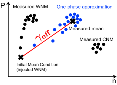
Figure 12: Schematic $P$-$n$ diagram to explain the concept of $\gamma_{\rm eff}$ formulated from our converging-flow simulations. The density of filled circles schematically represents the mass frequency in the shock-compressed layer (see Panels (a) and (b) of Figure 3.2). The bottom-left black cross shows the injected WNM state. In converging-flow simulations, the injected WNM is first adiabatically shocked (“Measured WNM”, black circles on the left) then cools to form CNM (“Measured CNM”, black circles on the right). As a result, we obtain the mean state averaged over the shock-compressed layer (“Measured mean”, the top-right black cross). $\gamma_{\rm eff}$ connects the initial WNM state and the mean state of the multiphase ISM (“$\gamma_{\rm eff}$”, the red solid line). The converging flow of an adiabatic WNM using the effective index $\gamma_{\rm eff}$ reproduces the mean state of the multiphase ISM without directly calculating the heating and cooling processes (“one-phase approximation”, blue circles).

Figure 13: Left: The time evolution of the effective index $\gamma_{\rm eff}$ as a function of time and $\Delta\rho_{0}$ with $\Delta x=0.02$ pc. The color corresponds to $\Delta\rho_{0}$ and the shades show the range of the maximum and minimum due to Phase $\alpha_{1}$, $\alpha_{2}$, and $\alpha_{3}$ in each $\Delta\rho_{0}$. Right: the time evolution of the average shock front position $\langle x_{\rm shock}\rangle$. “3D with cooling” (black line) shows $\langle x_{\rm shock}\rangle$ from $\Delta\rho_{0}=100$ % (Run C2D1000 with Phase $\alpha_{1}$), whereas “1D with $\gamma_{\rm eff}$” (red straight line) shows $\langle x_{\rm shock}\rangle$ of the test demonstration using $\gamma_{\rm eff}=0.863$ (Run E2D0000).

The left panel of Figure 2.2 shows the time evolution of $\gamma_{\rm eff}$. We measure the $V_{\rm shock}$ as $(x_{\rm shock}(t)-x_{\rm shock}(t-0.1\,\mathrm{Myr}))/0.1\,\mathrm{Myr}$ until $\tau_{\rm cool}$ (=1.3 Myr), and perform a linear fit as $(x_{\rm shock}(t)-x_{\rm shock}(\tau_{\rm cool}))/(t-\tau_{\rm cool})$ after $\tau_{\rm cool}$. All $\Delta\rho_{0}$ cases show a decreasing trend of $\gamma_{\rm eff}$ in time, which reflects the time-evolution of $\langle n\rangle$ due to the CNM formation (i.e., the layer becomes softer by forming CNM; see Figure 3.2). $\gamma_{\rm eff}$ tends to become constant after $\tau_{\rm cool}$ because the layer expansion becomes quasi-steady with an almost quasi-steady NM mass fraction (see the left panel of Figure 2.2). Larger/smaller $\Delta\rho_{0}$ cases have lower/higher mean density, and $\gamma_{\rm eff}$ is stiffer/softer accordingly, as we expected.

We found that $\gamma_{\rm eff}$ is softer than isothermal even in the stiffest case $\Delta\rho_{0}=100$ %, and that it becomes as soft as $\gamma_{\rm eff}\sim 0.7$ in smaller $\Delta\rho_{0}$ conditions. Such a high compressibility indicates that the overall dynamics on $<10$ pc scales in large-scale simulations could be further improved by introducing this type of the effective EoS, especially in regions where the multiphase ISM formation is ongoing without any feedback, because most of current simulations use $\gamma_{\rm eff}>1$ as a sub-grid model (c.f., Inoue & Yoshida 2019).

As the first step towards such an actual application, we perform a converging adiabatic WNM flow by employing $\gamma_{\rm eff}$ to demonstrate how well our $\gamma_{\rm eff}$ reproduces the properties of the multiphase ISM. In this demonstration, we directly update the thermal pressure based on the density evolution and $\gamma_{\rm eff}$ at each timestep, instead of calculating the heating and cooling ($\rho\mathcal{L}$ in Equation 3). For simplicity, we opt to solve equations only in the $x$ direction to set this demonstration of $\gamma_{\rm eff}$ in one-dimensional case, and set a constant value of $\gamma_{\rm eff}=0.863$ without modelling any time-evolution seen in the left panel of Figure 2.2. This value $0.863$ is based on the result of Run C2D1000 with Phase $\alpha_{1}$ at 3 Myr. We also employ $\Delta\rho_{0}=0$ to simulate a completely uniform head-on collision, just as an simple demonstration.

The right panel of Figure 2.2 shows the time evolution of $\langle x_{\rm shock}\rangle$. “3D with cooling” shows the result of our simulations with $\Delta\rho_{0}=100$ % (Run C2D1000 with Phase $\alpha_{1}$), whereas “1D with $\gamma_{\rm eff}$” shows the result of this the test demonstration using $\gamma_{\rm eff}=0.863$ (Run E2D0000). Table 2.2 summarizes the measured properties at 3 Myr. Our constant $\gamma_{\rm eff}$ does not reproduce the detailed time-evolution of “3D with cooling.” Nevertheless it successfully reproduces $V_{\rm in}+V_{\rm shock}$, $\langle x_{\rm shock}\rangle$, and $\langle n\rangle$ at 3 Myr within 11 % difference, which is still smaller than the variation due to different $\alpha$; for example, the variation of $\langle x_{\rm shock}\rangle$ due to Phases $\alpha_{1}$, $\alpha_{2}$, and $\alpha_{3}$ at 3 Myr is $1.763$ pc in Run C2D1000 ($\sim$ 29 % variation against $\langle x_{\rm shock}\rangle=6.183$ pc with Phase $\alpha_{1}$; see the shade of $\Delta\rho_{0}=100$ % in the left panel of Figure 2.2).

Ideally, we would like to provide a time-evolving model of $\gamma_{\rm eff}(t)$ along with a time-evolving model of $f_{\rm CNM}$, which, however, we reserve for future studies at this moment. In such studies, we should also consider the intrinsic variation of $\gamma_{\rm eff}$ due to random phases, for example, $\gamma_{\rm eff}=0.829$, $0.863$, and $0.898$ in Run C2D1000 with Phases $\alpha_{3}$, $\alpha_{1}$, and $\alpha_{2}$ at 3 Myr (see the left panel of Figure 2.2).

Table 3: Measured Properties at 3 Myr

Note. $V_{\rm in}+V_{\rm shock}$, $\langle x_{\rm shock}\rangle$, and $\langle n\rangle$ measured in Runs C2D1000 and E2D0000.

Note that the implementation of this effective EoS is unfortunately not that straightforward. For example, to introduce a time-evolving $\gamma_{\rm eff}$, we would like to measure shock propagation speed and elapsed-time since the last shock passage even in large-scale simulations. This is, however, computationally expensive and time-consuming, similar to following stellar population evolution below the spatial resolution to blow supernovae at a correct timing. Such difficulties have to be also discussed and left for future studies. Nevertheless, since the typical frequency of shock passages is as high as once per Myr (e.g., McKee & Ostriker 1977, ; see also Section 4.6), we may expect that the quasi-steady $\gamma_{\rm eff}$ at $\sim 3$ Myr is still close to the typical time-averaged state of the actual ISM.

4.6 Limitations of Current Converging Flow Systems

In this section, we briefly address some potential limitations/issues in converging flow simulations (not only ours but also in general). Given that 1 Myr is the typical interval in the ISM between successive shock passages by multiple supernovae and/or H ii regions (McKee & Ostriker 1977; Inutsuka et al. 2015), supersonic flow in reality continue in a fixed direction only $\leq$ 1 Myr. Statistically speaking, successive flows essentially propagate from any direction and they incident the shock-compressed layer at some angle. Almost all of the converging flow studies therefore presumably keep the flow injection too long in a fixed direction. There are previous studies introducing an inclination angle between flows to investigate the effect of magnetic diffusion and supercritical core formation (Körtgen & Banerjee 2015) and to investigate the reorientation of pre-existing filaments (c.f., Fogerty et al. 2016, 2017), but it is still left for future studies to reveal how the mean properties of the shock-compressed layer depend on such inclinations and multiple compressions by flows from various angles.

Similarly, the typical dynamical timescale of the shock-compressed layer is a few Myr (e.g., the crossing time of the WNM component over the shock-compressed layer is $10$ pc / $10{\rm km\,s^{-1}}$ in Run C2D1000). It is thus also left for future studies to investigate how an already-created shock-compressed layer expands and/or shrinks once the inflow ceases and to measure whether the turbulence and $f_{\rm CNM}$ is maintained or not. Limiting the inflow mass is one of the technique to study such condition; Vázquez-Semadeni et al. (2007) for example demonstrate that the global and local collapses of the shock-compressed layers occur once all the gas finish accreting onto the shock-compressed layers.

The concept of converging flow setup is to easily perform calculations in the post-shock rest frame. However, most of the post-shock regions in reality is presumably not sandwiched by two shock fronts as in the converging flows, but instead by one shock front and one contact discontinuity. Converging flow is just an analogue of such a shock-contact discontinuity system, and only one half side of shock-compressed layer is meaningful. The two-shock-front configuration likely impacts the time-evolution of the shock-compressed layer. For example as shown in Figure 2.2, fast WNM flows continue deep into the layer and interact each other, especially when $\Delta\rho_{0}$ is large, which depends on the shock front geometry on both two sides. The turbulent properties and $f_{\rm CNM}$ may accordingly differ in a shock-contact discontinuity system. Simulation studies of a shock-contact discontinuity system (e.g., Koyama & Inutsuka 2002) is still limited and careful comparison is left for future studies.

We also ignore magnetic fields for simplicity in this article, but they play a pivotal role; for example magnetic field pressure supports the shock-compressed layer and the turbulence decays, especially in case the field lines have perpendicular orientation against the inflow (Heitsch et al. 2009; Vázquez-Semadeni et al. 2011; Inoue & Inutsuka 2012; Iwasaki et al. 2019). We expect that magnetic fileds do not modify our proposed $\gamma_{\rm eff}$ significantly because the magnetized shock-compressed layer tends to be equipartition (see Iwasaki et al. 2019, for $V_{\rm in}<20\,{\rm km\,s^{-1}}$ cases), but this still has to be investigated with magnetized converging flow simulations.

5 Summary

We perform a series of hydrodynamics simulations of converging warm neutral medium (WNM) flows with heating and cooling, to calculate the cold neutral medium (CNM) formation and to investigate the mean physical properties of the multiphase interstellar medium (ISM) averaged over the shock-compressed layer on a 10 pc scale, such as the mean shock front position $\langle x_{\rm shock}\rangle$, the mean density $\langle n\rangle$, and the density-weighted velocity dispersion $\sqrt{\langle\delta v_{\rm dw}^{2}\rangle_{\rm tot}}$. Under a fixed flow velocity of $20{\rm km\,s^{-1}}$ and the Kolmogorov power spectrum in the upstream density fluctuation, we systematically vary the amplitude of the upstream density fluctuation $\Delta\rho_{0}=\sqrt{\langle\delta\rho_{0}\rangle}/\rho_{0}$, random phases of the fluctuation $\alpha$, and the spatial resolution $\Delta x$. We find that two distinct post-shock states exist depending on $\Delta\rho_{0}$, typically divided by $\Delta\rho_{0}=10$ %. We list our main findings as follows.

1. The convergence in $\langle x_{\rm shock}\rangle$ and $\langle n\rangle$ requires $\Delta x=0.02$ pc by fully resolving the typical cooling length on which the phase transition occurs from the WNM to CNM.

2. The trend of convergence, however, differs depending on $\Delta\rho_{0}$. The trend is non-monotonic when $\Delta\rho_{0}>10$ % due to the intrinsic large variation induced by different phase $\alpha$ and different $\Delta x$, and calculations with coarse resolutions of $\Delta x>0.02$ pc practically provide simliar values in $\langle x_{\rm shock}\rangle$ and $\langle n\rangle$. The convergence in the case of $\Delta\rho_{0}\leq 10$ % is monotonic and stringently requires $\Delta x=0.02$ pc.

3. The significant deformation of the shock fronts in large $\Delta\rho_{0}$ cases drive strong turbulence up to $\sqrt{\langle\delta v_{\rm dw}^{2}\rangle_{\rm tot}}\sim 7\,{\rm km\,s^{-1}}$, which prevents the dynamical condensation by cooling and the CNM formation. When $\Delta\rho_{0}$ is small, the shock fronts maintain a straight geometry and the velocity dispersion is limited to the thermal-instability mediated level of $\sqrt{\langle\delta v_{\rm dw}^{2}\rangle_{\rm tot}}=2$ – $3\,{\rm km\,s^{-1}}$.

4. The shock-compressed layer is wider (narrower) and less dense (denser) with larger (smaller) $\Delta\rho_{0}$, where the CNM mass fraction is $\sim 45$ % and $\sim 70$ % when $\Delta\rho_{0}=31.6$ % and $3.16$ %, respectively.

5. The turbulent energy supports the shock-compressed layer when $\Delta\rho_{0}>10$ %, whereas both the turbulent and thermal energy equally supports the shock-compressed layer when $\Delta\rho_{0}\leq 10$ %.

6. We formulate an effective equation of state, $P\propto\rho^{\gamma_{\rm eff}}$, which approximates the multiphase ISM as a one-phase medium. $\gamma_{\rm eff}$ measured from our converging-flow simulations ranges from $0.9$ (with large $\Delta\rho_{0}$) to $0.7$ (with small $\Delta\rho_{0}$), softer than isothermal.

These results have to be further investigated by simulating other shock orientations, ceasing of mass accretion, and by including magnetic fields as well as in a shock-contact discontinuity system. We also hope that upcoming observations (e.g., ALMA, SKA, ngVLA) constrain the formation condition of the multiphase ISM, such as $\Delta\rho_{0}$, by measuring the physical properties of the ISM (velocity dispersion, the CNM mass fraction, etc.).

ACKNOWLEDGMENTS

We are grateful to the anonymous reviewer for his/her careful reading and comments, which improved our manuscript significantly. Numerical computations were carried out on Cray XC30 and XC50 at Center for Computational Astrophysics, National Astronomical Observatory of Japan. MINK (15J04974, 18J00508, 20H04739), TI (18H05436, 20H01944), SI (16H02160, 18H05436, 18H05437), KT (16H05998, 16K13786,17KK0091), KI (19K03929), and KEIT (19H05080, 19K14760) are supported by Grants-in-Aid from the Ministry of Education, Culture, Sports, Science, and Technology of Japan. KT and KEIT are also supported by NAOJ ALMA Scientific Research grant No. 2017-05A. MINK is grateful to Eve C. Ostriker, Woong-Tae Kim, Patrick Hennebelle, Philippe André, Marc-Antoine Miville-Deschênes, Antoine Marchal, Jin Koda, Kentaro Nagamine, Tomoyuki Hanawa, Kazuyuki Omukai, and Shinsuke Takasao for fruitful comments.

References

- Arata et al. (2018) Arata, S., Yajima, H., & Nagamine, K. 2018, MNRAS, 475, 4252, doi: 10.1093/mnras/sty122
- Armstrong et al. (1995) Armstrong, J. W., Rickett, B. J., & Spangler, S. R. 1995, ApJ, 443, 209, doi: 10.1086/175515
- Audit & Hennebelle (2005) Audit, E., & Hennebelle, P. 2005, A&A, 433, 1, doi: 10.1051/0004-6361:20041474
- Audit & Hennebelle (2008) Audit, E., & Hennebelle, P. 2008, in Astronomical Society of the Pacific Conference Series, Vol. 385, Numerical Modeling of Space Plasma Flows, ed. N. V. Pogorelov, E. Audit, & G. P. Zank, 73
- Baba et al. (2017) Baba, J., Morokuma-Matsui, K., & Saitoh, T. R. 2017, MNRAS, 464, 246, doi: 10.1093/mnras/stw2378
- Balbus (1986) Balbus, S. A. 1986, ApJ, 303, L79, doi: 10.1086/184657
- Balbus (1995) —. 1995, ApJ, 453, 380, doi: 10.1086/176397
- Birnboim et al. (2015) Birnboim, Y., Balberg, S., & Teyssier, R. 2015, MNRAS, 447, 3678, doi: 10.1093/mnras/stu2717
- Bonnell et al. (2013) Bonnell, I. A., Dobbs, C. L., & Smith, R. J. 2013, MNRAS, 430, 1790, doi: 10.1093/mnras/stt004
- Burkhart et al. (2015) Burkhart, B., Lee, M.-Y., Murray, C. E., & Stanimirović, S. 2015, ApJ, 811, L28, doi: 10.1088/2041-8205/811/2/L28
- Carroll-Nellenback et al. (2014) Carroll-Nellenback, J. J., Frank, A., & Heitsch, F. 2014, ApJ, 790, 37, doi: 10.1088/0004-637X/790/1/37
- Chepurnov & Lazarian (2010) Chepurnov, A., & Lazarian, A. 2010, ApJ, 710, 853, doi: 10.1088/0004-637X/710/1/853
- Chevalier (1977) Chevalier, R. A. 1977, ARA&A, 15, 175, doi: 10.1146/annurev.aa.15.090177.001135
- Chevalier (1999) —. 1999, ApJ, 511, 798, doi: 10.1086/306710
- Colling et al. (2018) Colling, C., Hennebelle, P., Geen, S., Iffrig, O., & Bournaud, F. 2018, A&A, 620, A21, doi: 10.1051/0004-6361/201833161
- Cox & Tucker (1969) Cox, D. P., & Tucker, W. H. 1969, ApJ, 157, 1157, doi: 10.1086/150144
- Dalgarno & McCray (1972) Dalgarno, A., & McCray, R. A. 1972, ARA&A, 10, 375, doi: 10.1146/annurev.aa.10.090172.002111
- Field (1965) Field, G. B. 1965, ApJ, 142, 531, doi: 10.1086/148317
- Field et al. (1969) Field, G. B., Goldsmith, D. W., & Habing, H. J. 1969, ApJ, 155, L149, doi: 10.1086/180324
- Fogerty et al. (2017) Fogerty, E., Carroll-Nellenback, J., Frank, A., Heitsch, F., & Pon, A. 2017, MNRAS, 470, 2938, doi: 10.1093/mnras/stx1381
- Fogerty et al. (2016) Fogerty, E., Frank, A., Heitsch, F., et al. 2016, MNRAS, 460, 2110, doi: 10.1093/mnras/stw1141
- Fukui et al. (2018) Fukui, Y., Hayakawa, T., Inoue, T., et al. 2018, ApJ, 860, 33, doi: 10.3847/1538-4357/aac16c
- Gatto et al. (2017) Gatto, A., Walch, S., Naab, T., et al. 2017, MNRAS, 466, 1903, doi: 10.1093/mnras/stw3209
- Gent et al. (2013) Gent, F. A., Shukurov, A., Fletcher, A., Sarson, G. R., & Mantere, M. J. 2013, MNRAS, 432, 1396, doi: 10.1093/mnras/stt560
- Girichidis et al. (2016) Girichidis, P., Walch, S., Naab, T., et al. 2016, MNRAS, 456, 3432, doi: 10.1093/mnras/stv2742
- Heitsch et al. (2005) Heitsch, F., Burkert, A., Hartmann, L. W., Slyz, A. D., & Devriendt, J. E. G. 2005, ApJ, 633, L113, doi: 10.1086/498413
- Heitsch et al. (2006) Heitsch, F., Slyz, A. D., Devriendt, J. E. G., Hartmann, L. W., & Burkert, A. 2006, ApJ, 648, 1052, doi: 10.1086/505931
- Heitsch et al. (2009) Heitsch, F., Stone, J. M., & Hartmann, L. W. 2009, ApJ, 695, 248, doi: 10.1088/0004-637X/695/1/248
- Hennebelle (2018) Hennebelle, P. 2018, A&A, 611, A24, doi: 10.1051/0004-6361/201731071
- Hennebelle & Audit (2007) Hennebelle, P., & Audit, E. 2007, A&A, 465, 431, doi: 10.1051/0004-6361:20066139
- Hennebelle et al. (2008) Hennebelle, P., Banerjee, R., Vázquez-Semadeni, E., Klessen, R. S., & Audit, E. 2008, A&A, 486, L43, doi: 10.1051/0004-6361:200810165
- Hennebelle & Iffrig (2014) Hennebelle, P., & Iffrig, O. 2014, A&A, 570, A81, doi: 10.1051/0004-6361/201423392
- Hennebelle & Pérault (1999) Hennebelle, P., & Pérault, M. 1999, A&A, 351, 309
- Hennebelle & Pérault (2000) —. 2000, A&A, 359, 1124
- Heyer & Brunt (2004) Heyer, M. H., & Brunt, C. M. 2004, ApJ, 615, L45, doi: 10.1086/425978
- Ho et al. (2019) Ho, S. H., Martin, C. L., & Turner, M. L. 2019, ApJ, 875, 54, doi: 10.3847/1538-4357/ab0ec2
- Inoue & Yoshida (2019) Inoue, S., & Yoshida, N. 2019, MNRAS, 488, 4400, doi: 10.1093/mnras/stz2076
- Inoue & Inutsuka (2008) Inoue, T., & Inutsuka, S.-i. 2008, ApJ, 687, 303, doi: 10.1086/590528
- Inoue & Inutsuka (2009) —. 2009, ApJ, 704, 161, doi: 10.1088/0004-637X/704/1/161
- Inoue & Inutsuka (2012) —. 2012, ApJ, 759, 35, doi: 10.1088/0004-637X/759/1/35
- Inoue & Inutsuka (2016) —. 2016, ApJ, 833, 10, doi: 10.3847/0004-637X/833/1/10
- Inoue & Omukai (2015) Inoue, T., & Omukai, K. 2015, ApJ, 805, 73, doi: 10.1088/0004-637X/805/1/73
- Inoue et al. (2013) Inoue, T., Shimoda, J., Ohira, Y., & Yamazaki, R. 2013, ApJ, 772, L20, doi: 10.1088/2041-8205/772/2/L20
- Inoue et al. (2012) Inoue, T., Yamazaki, R., Inutsuka, S.-i., & Fukui, Y. 2012, ApJ, 744, 71, doi: 10.1088/0004-637X/744/1/71
- Inutsuka et al. (2015) Inutsuka, S.-i., Inoue, T., Iwasaki, K., & Hosokawa, T. 2015, A&A, 580, A49, doi: 10.1051/0004-6361/201425584
- Iwasaki & Inutsuka (2012) Iwasaki, K., & Inutsuka, S.-i. 2012, MNRAS, 423, 3638, doi: 10.1111/j.1365-2966.2012.21156.x
- Iwasaki & Inutsuka (2014) —. 2014, ApJ, 784, 115, doi: 10.1088/0004-637X/784/2/115
- Iwasaki et al. (2019) Iwasaki, K., Tomida, K., Inoue, T., & Inutsuka, S.-i. 2019, ApJ, 873, 6, doi: 10.3847/1538-4357/ab02ff
- Joshi et al. (2019) Joshi, P. R., Walch, S., Seifried, D., et al. 2019, MNRAS, 484, 1735, doi: 10.1093/mnras/stz052
- Joung et al. (2009) Joung, M. R., Mac Low, M.-M., & Bryan, G. L. 2009, ApJ, 704, 137, doi: 10.1088/0004-637X/704/1/137
- Kennicutt & Evans (2012) Kennicutt, R. C., & Evans, N. J. 2012, ARA&A, 50, 531, doi: 10.1146/annurev-astro-081811-125610
- Kim & Ostriker (2015) Kim, C.-G., & Ostriker, E. C. 2015, ApJ, 802, 99, doi: 10.1088/0004-637X/802/2/99
- Kim & Ostriker (2017) —. 2017, ApJ, 846, 133, doi: 10.3847/1538-4357/aa8599
- Kim et al. (2017) Kim, C.-G., Ostriker, E. C., & Raileanu, R. 2017, ApJ, 834, 25, doi: 10.3847/1538-4357/834/1/25
- Kim et al. (2020) Kim, W.-T., Kim, C.-G., & Ostriker, E. C. 2020, ApJ, 898, 35, doi: 10.3847/1538-4357/ab9b87
- Kolmogorov (1941) Kolmogorov, A. 1941, Akademiia Nauk SSSR Doklady, 30, 301
- Körtgen & Banerjee (2015) Körtgen, B., & Banerjee, R. 2015, MNRAS, 451, 3340, doi: 10.1093/mnras/stv1200
- Koyama & Inutsuka (2000) Koyama, H., & Inutsuka, S.-I. 2000, ApJ, 532, 980, doi: 10.1086/308594
- Koyama & Inutsuka (2002) Koyama, H., & Inutsuka, S.-i. 2002, ApJ, 564, L97, doi: 10.1086/338978
- Koyama & Inutsuka (2004) —. 2004, ApJ, 602, L25, doi: 10.1086/382478
- Koyama & Inutsuka (2006) —. 2006, arXiv e-prints, arXiv:0605528. https://arxiv.org/abs/0605528
- Larson (1981) Larson, R. B. 1981, MNRAS, 194, 809, doi: 10.1093/mnras/194.4.809
- Lazarian & Pogosyan (2000) Lazarian, A., & Pogosyan, D. 2000, ApJ, 537, 720, doi: 10.1086/309040
- McCray & Snow (1979) McCray, R., & Snow, T. P., J. 1979, ARA&A, 17, 213, doi: 10.1146/annurev.aa.17.090179.001241
- McKee & Ostriker (1977) McKee, C. F., & Ostriker, J. P. 1977, ApJ, 218, 148, doi: 10.1086/155667
- Micic et al. (2013) Micic, M., Glover, S. C. O., Banerjee, R., & Klessen, R. S. 2013, MNRAS, 432, 626, doi: 10.1093/mnras/stt489
- Nishihara et al. (2010) Nishihara, K., Wouchuk, J. G., Matsuoka, C., Ishizaki, R., & Zhakhovsky, V. V. 2010, Philosophical Transactions of the Royal Society of London Series A, 368, 1769, doi: 10.1098/rsta.2009.0252
- Ntormousi et al. (2017) Ntormousi, E., Dawson, J. R., Hennebelle, P., & Fierlinger, K. 2017, A&A, 599, A94, doi: 10.1051/0004-6361/201629268
- Parker (1953) Parker, E. N. 1953, ApJ, 117, 431, doi: 10.1086/145707
- Patra et al. (2018) Patra, N. N., Kanekar, N., Chengalur, J. N., & Roy, N. 2018, MNRAS, 479, L7, doi: 10.1093/mnrasl/sly087
- Richtmyer (1960) Richtmyer, R. D. 1960, Commun. Pure Appl. Math., 13, 297
- Schneider et al. (2013) Schneider, N., André, P., Könyves, V., et al. 2013, ApJ, 766, L17, doi: 10.1088/2041-8205/766/2/L17
- Schneider et al. (2016) Schneider, N., Bontemps, S., Motte, F., et al. 2016, A&A, 587, A74, doi: 10.1051/0004-6361/201527144
- Shu et al. (1972) Shu, F. H., Milione, V., Gebel, W., et al. 1972, ApJ, 173, 557, doi: 10.1086/151444
- Springel & Hernquist (2003) Springel, V., & Hernquist, L. 2003, MNRAS, 339, 289, doi: 10.1046/j.1365-8711.2003.06206.x
- Tomisaka et al. (1981) Tomisaka, K., Habe, A., & Ikeuchi, S. 1981, Ap&SS, 78, 273, doi: 10.1007/BF00648941
- Tomisaka & Ikeuchi (1986) Tomisaka, K., & Ikeuchi, S. 1986, PASJ, 38, 697
- Valdivia et al. (2016) Valdivia, V., Hennebelle, P., Gérin, M., & Lesaffre, P. 2016, A&A, 587, A76, doi: 10.1051/0004-6361/201527325
- van Leer (1979) van Leer, B. 1979, Journal of Computational Physics, 32, 101, doi: 10.1016/0021-9991(79)90145-1
- van Loo et al. (2010) van Loo, S., Falle, S. A. E. G., & Hartquist, T. W. 2010, MNRAS, 406, 1260, doi: 10.1111/j.1365-2966.2010.16761.x
- van Loo et al. (2007) van Loo, S., Falle, S. A. E. G., Hartquist, T. W., & Moore, T. J. T. 2007, A&A, 471, 213, doi: 10.1051/0004-6361:20077430
- Vázquez-Semadeni et al. (2011) Vázquez-Semadeni, E., Banerjee, R., Gómez, G. C., et al. 2011, MNRAS, 414, 2511, doi: 10.1111/j.1365-2966.2011.18569.x
- Vázquez-Semadeni et al. (2007) Vázquez-Semadeni, E., Gómez, G. C., Jappsen, A. K., et al. 2007, ApJ, 657, 870, doi: 10.1086/510771
- Vázquez-Semadeni et al. (2006) Vázquez-Semadeni, E., Ryu, D., Passot, T., González, R. F., & Gazol, A. 2006, ApJ, 643, 245, doi: 10.1086/502710
- Wada et al. (2011) Wada, K., Baba, J., & Saitoh, T. R. 2011, ApJ, 735, 1, doi: 10.1088/0004-637X/735/1/1
- Wada & Norman (1999) Wada, K., & Norman, C. A. 1999, ApJ, 516, L13, doi: 10.1086/311987
- Walch et al. (2015) Walch, S., Girichidis, P., Naab, T., et al. 2015, MNRAS, 454, 238, doi: 10.1093/mnras/stv1975
- Wolfire et al. (1995) Wolfire, M. G., Hollenbach, D., McKee, C. F., Tielens, A. G. G. M., & Bakes, E. L. O. 1995, ApJ, 443, 152, doi: 10.1086/175510
- Wolfire et al. (2003) Wolfire, M. G., McKee, C. F., Hollenbach, D., & Tielens, A. G. G. M. 2003, ApJ, 587, 278, doi: 10.1086/368016
- Yepes et al. (1997) Yepes, G., Kates, R., Khokhlov, A., & Klypin, A. 1997, MNRAS, 284, 235, doi: 10.1093/mnras/284.1.235
- Zel’dovich & Pikel’ner (1969) Zel’dovich, Y. B., & Pikel’ner, S. B. 1969, Soviet Journal of Experimental and Theoretical Physics, 29, 170