Sub-linear convergence of a stochastic proximal iteration method in Hilbert space

Abstract.

We consider a stochastic version of the proximal point algorithm for optimization problems posed on a Hilbert space. A typical application of this is supervised learning. While the method is not new, it has not been extensively analyzed in this form. Indeed, most related results are confined to the finite-dimensional setting, where error bounds could depend on the dimension of the space. On the other hand, the few existing results in the infinite-dimensional setting only prove very weak types of convergence, owing to weak assumptions on the problem. In particular, there are no results that show convergence with a rate. In this article, we bridge these two worlds by assuming more regularity of the optimization problem, which allows us to prove convergence with an (optimal) sub-linear rate also in an infinite-dimensional setting. In particular, we assume that the objective function is the expected value of a family of convex differentiable functions. While we require that the full objective function is strongly convex, we do not assume that its constituent parts are so. Further, we require that the gradient satisfies a weak local Lipschitz continuity property, where the Lipschitz constant may grow polynomially given certain guarantees on the variance and higher moments near the minimum. We illustrate these results by discretizing a concrete infinite-dimensional classification problem with varying degrees of accuracy.

1. Introduction

We consider convex optimization problems of the form

(1.1) $$w^{*}=\operatorname*{arg\,min}_{w\in H}F(w),$$

where

$$F(w)=\mathbf{E}_{\xi}[f(w,\xi)].$$

The main applications we have in mind are supervised learning tasks. In such a problem, a set of data samples $\{x_{j}\}_{j=1}^{n}$ with corresponding labels $\{y_{j}\}_{j=1}^{n}$ is given, as well as a classifier $h$ depending on the parameters $w$. The goal is to find $w$ such that $h(w,x_{j})\approx y_{j}$ for all $j\in\{1,\dots,n\}$. This is done by minimizing

(1.2) $$F(w)=\frac{1}{n}\sum_{j=1}^{n}{\ell(h(w,x_{j}),y_{j})},$$

where $\ell$ is a given loss function. We refer to, e.g., Bottou, Curtis & Nocedal [9] for an overview. In order to reduce the computational costs, it has been proved to be useful to split $F$ into a collection of functions $f$ of the type

$$f(w,\xi)=\frac{1}{|B_{\xi}|}\sum_{j\in B_{\xi}}{\ell(h(w,x_{j}),y_{j})},$$

where $B_{\xi}$ is a random subset of $\{1,\dots,n\}$, referred to as a batch. In particular, the case of $|B_{\xi}|=1$ is interesting for applications, as it corresponds to a separation of the data into single samples.

A commonly used method for such problems is the stochastic gradient method (SGD), given by the iteration

$$w^{k+1}=w^{k}-\alpha_{k}\nabla f(w^{k},\xi^{k}),$$

where $\alpha_{k}>0$ denotes a step size, $\{\xi^{k}\}_{k\in\mathbb{N}}$ is a family of jointly independent random variables and $\nabla$ denotes the Gâteaux derivative with respect to the first variable. The idea is that in each step we choose a random part $f(\cdot,\xi)$ of $F$ and go in the direction of the negative gradient of this function. SGD corresponds to a stochastic version of the explicit (forward) Euler scheme applied to the gradient flow

$$\dot{w}=-\nabla F(w).$$

This differential equation is frequently stiff, which means that the method often suffers from stability issues.

The restatement of the problem as a gradient flow suggests that we could avoid such stability problems by instead considering a stochastic version of implicit (backward) Euler, given by

$$w^{k+1}=w^{k}-\alpha_{k}\nabla f(w^{k+1},\xi^{k}).$$

In the deterministic setting, this method has a long history under the name proximal point method, because it is equivalent to

$$w^{k+1}=\operatorname*{arg\,min}_{w\in H}\Big{\{}\alpha F(w)+\frac{1}{2}\|w-w^{k}\|^{2}\Big{\}}=\text{prox}_{\alpha F}(w^{k}),$$

where

$$\text{prox}_{\alpha F}(w^{k})=(I+\alpha\nabla F)^{-1}w^{k}.$$

The proximal point method has been studied extensively in the infinite dimensional but deterministic case, beginning with the work of Rockafellar [26]. Several convergence results and connections to other methods such as the Douglas–Rachford splitting are collected in Eckstein & Bertsekas [13].

Following Ryu & Boyd [29], we will refer to the stochastic version as stochastic proximal iteration (SPI). We note that the computational cost of one SPI step is in general much higher than for SGD, and indeed often infeasible. However, in many special cases a clever reformulation can result in very similar costs. If so, then SPI should be preferred over SGD, as it will converge more reliably. We provide such an example in Section 5.

The main goal of this paper is to prove sub-linear convergence of the type

$$\mathbf{E}\big{[}\|w^{k}-w^{*}\|^{2}\big{]}\leq\frac{C}{k}$$

in an infinite-dimensional setting, i.e. where $\{w^{k}\}_{k\in\mathbb{N}}$ and $w^{*}$ are elements in a Hilbert space $H$. As shown in e.g. [1, 24], this is optimal in the sense that we cannot expect a better asymptotic rate even in the finite-dimensional case.

Most previous convergence results in this setting only provide guarantees for convergence, without an explicit error bound. The convergence is usually also in a rather weak norm. This is mainly due to weak assumptions on the involved functions and operators. Overall, little work has been done to consider SPI in an infinite dimensional space. A few exceptions are given by Bianchi [7], where maximal monotone operators $\nabla F\colon H\to 2^{H}$ are considered and weak ergodic convergence and norm convergence is proved. In Rosasco et al. [28], the authors work with an infinite dimensional setting and an implicit-explicit splitting where $\nabla F$ is decomposed in a regular and an irregular part. The regular part is considered explicitly but with a stochastic approximation while the irregular part is used in a deterministic proximal step. They prove both $\nabla F(w^{k})\to\nabla F(w^{*})$ and $w^{k}\to w^{*}$ in $H$ as $k\to\infty$. Without further assumptions, neither of these approaches yield convergence rates.

In the finite-dimensional case, stronger assumptions are typically made, with better convergence guarantees as a result. Nevertheless, for the SPI scheme in particular, we are only aware of the unpublished manuscript [29], which suggests $\nicefrac{{1}}{{k}}$ convergence in $\mathbb{R}^{d}$. Based on [29], the implicit method has also been considered in a few other works: In Patrascu & Necoara [22], a SPI method with additional constraints on the domain was studied. A slightly more general setting that includes the SPI has been considered in Davis & Drusvyatskiy [12]. Toulis & Airoldi and Toulis et al. studied such an implicit scheme in [33, 34, 32].

Whenever using an implicit scheme, it is essential to solve the appearing implicit equation effectively. This can be impeded by large batches for the stochastic approximation of $F$. On the other hand, a larger batch improves the accuracy of the approximation of the function. In Toulis, Tran & Airoldi [36, 37] and Ryu & Yin [30], a compromise was found by solving several implicit problems on small batches and taking the average of these results. This corresponds to a sum splitting. Furthermore, implicit-explicit splittings can be found in Patrascu & Irofti [21], Ryu & Yin [30], Salim et al. [31], Bianchi & Hachem [8] and Bertsekas [6]. A few more related schemes have been considered in Asi & Duchi [2, 3] and Toulis, Horel & Airoldi [35]. More information about the complexity of solving these kinds of implicit equations and the corresponding implementation can be found in Fagan & Iyengar [16] and Tran, Toulis & Airoldi in [37].

Our aim is to bridge the gap between the “strong finite-dimensional” and “weak infinite-dimensional” settings, by extending the approach of [29] to the infinite-dimensional case. We also further extend the results by allowing for more general Lipschitz conditions on $\nabla f(\cdot,\xi)$, provided that sufficient guarantees can be made on the integrability near the minimum $w^{*}$. These strong convergence results can then be applied to, e.g., the setting where there is an original infinite-dimensional optimization problem which is subsequently discretized into a series of finite-dimensional problems. Given a reasonable discretization, each of those problems will then satisfy the same convergence guarantees. We will follow [29] closely, because their approach is sound. However, several arguments no longer work in the infinite-dimensional case (such as the unit ball being compact, or a linear operator having a minimal eigenvalue) and we fix those. Additionally, we simplify several of the remaining arguments, provide many omitted, but critical, details and extend the results to less bounded operators.

A brief outline of the paper is as follows. The main assumptions that we make are stated in Section 2, as well as the main theorem. Then we prove a number of preliminary results in Section 3, before we can tackle the main proof in Section 4. In Section 5 we describe a numerical experiment that illustrates our results, and then we summarize our findings in Section 6.

2. Assumptions and main theorem

Let $(\Omega,\mathcal{F},\mathbf{P})$ be a complete probability space and let $\{\xi^{k}\}_{k\in\mathbb{N}}$ be a family of jointly independent random variables on $\Omega$. Each realization of $\xi^{k}$ corresponds to a different batch. Let $(H,(\cdot,\cdot),\|\cdot\|)$ be a real Hilbert space and $(H^{*},(\cdot,\cdot)_{H^{*}},\|\cdot\|_{H^{*}})$ its dual. Since $H$ is a Hilbert space, there exists an isometric isomorphism $\iota\colon H^{*}\to H$ such that $\iota^{-1}\colon H\to H^{*}$ with $\iota^{-1}:u\mapsto(u,\cdot)$. Furthermore, the dual pairing is denoted by $\langle u^{\prime},u\rangle=u^{\prime}(u)$ for $u^{\prime}\in H^{*}$ and $u\in H$. It satisfies

$$\langle\iota^{-1}u,v\rangle=(u,v)\quad\text{and}\quad\langle u^{\prime},v\rangle=(\iota u^{\prime},v),\quad u,v\in H,u^{\prime}\in H^{*}.$$

We denote the space of linear bounded operators mapping $H$ into $H$ by $\mathcal{L}(H)$. For a symmetric operator $S$, we say that it is positive if $(Su,u)\geq 0$ for all $u\in H$. It is called strictly positive if $(Su,u)>0$ for all $u\in H$ such that $u\neq 0$.

For the function $f(\cdot,\xi)\colon H\times\Omega\to(-\infty,\infty]$, we use $\nabla$, as in $\nabla f(u,\xi)$, to denote differentiation with respect to the first variable. When we present an argument that holds almost surely, we will frequently omit $\xi$ from the notation and simply write $f(u)$ rather than $f(u,\xi)$. Given a random variable $X$ on $\Omega$, we denote the expectation with respect to $\mathbf{P}$ by $\mathbf{E}[X]$. We use sub-indices, such as in $\mathbf{E}_{\xi}[\cdot]$, to denote expectations with respect to the probability distribution of a certain random variable.

For the family of jointly independent random variables $\{\xi^{k}\}_{k\in\mathbb{N}}$, we are interested in the total expectation

$$\mathbf{E}_{k}\big{[}\|X\|^{2}\big{]}=\mathbf{E}_{\xi^{1}}\big{[}\mathbf{E}_{\xi^{2}}\big{[}\cdots\mathbf{E}_{\xi^{k}}\big{[}\|X\|^{2}\big{]}\cdots\big{]}\big{]}.$$

Since the random variables $\{\xi^{k}\}_{k\in\mathbb{N}}$ are jointly independent, and $w^{k}$ only depends on $\xi^{j}$, $j\leq k-1$, this expectation coincides with the expectation with respect to the joint probability distribution of $\xi^{1},\ldots,\xi^{k-1}$. In the rest of the paper, it often occurs that a statement does not involve an expectation but contains a random variable. Where it does not cause any confusion, such a statement is assumed to hold almost surely even if this is not explicitly stated.

We consider the stochastic proximal iteration (SPI) scheme given by

(2.1) $$w^{k+1}=w^{k}-\alpha_{k}\iota\nabla f(w^{k+1},\xi^{k})\quad\text{ in }H,\quad\quad w^{1}=w_{1}\quad\text{ in }H,$$

for minimizing

$$F(w)=\mathbf{E}_{\xi}[f(w,\xi)],$$

where $f$ and $F$ fulfill the following assumption.

Assumption 1.

For a random variable $\xi$ on $\Omega$, let the function $f(\cdot,\xi)\colon\Omega\times H\to(-\infty,\infty]$ be given such that $f(\cdot,\xi)$ is convex, lower semi-continuous and proper almost surely. Additionally, $f(\cdot,\xi)$ fulfills the following conditions:

• The expectation $\mathbf{E}_{\xi}\big{[}f(\cdot,\xi)\big{]}=:F(\cdot)$ is lower semi-continuous and proper.

• The function $f(\cdot,\xi)$ is Gâteaux differentiable almost surely on a non-empty common domain $\mathcal{D}\left(\nabla f\right)\subseteq H$, i.e. for all for all $v,w\in\mathcal{D}\left(\nabla f\right)$ the inequality $\langle\iota\nabla f(v,\xi),w\rangle=\lim_{h\to 0}\frac{f(v+hw,\xi)-f(v,\xi)}{h}$ is fulfilled almost surely.

• There exists $m\in\mathbb{N}$ such that $\big{(}\mathbf{E}_{\xi}\big{[}\|\nabla f(w^{*},\xi)\|_{H^{*}}^{2^{m}}\big{]}\big{)}^{2^{-m}}=:\sigma<\infty$.

• For every $R>0$ there exists $L_{\xi}(R)\colon\Omega\to\mathbb{R}$ such that

  $$\|\nabla f(u,\xi)-\nabla f(v,\xi)\|_{H^{*}}\leq L_{\xi}(R)\|u-v\|$$

  almost surely for all $u,v\in\mathcal{D}\left(\nabla f\right)$ with $\|u\|,\|v\|\leq R$. Furthermore, there exists a polynomial $P\colon\mathbb{R}\to\mathbb{R}$ of degree $2^{m}-2$ such that $L_{\xi}(R)\leq P(R)$ almost surely.

• There exist a random variable $M_{\xi}\colon\Omega\to\mathcal{L}(H)$ such that the image is symmetric and a random variable $\mu_{\xi}\colon\Omega\to[0,\infty)$ such that $\mathbf{E}_{\xi}[\mu_{\xi}]=\mu>0$ and $\mathbf{E}_{\xi}[\mu_{\xi}^{2}]=\nu^{2}<\infty$. Moreover,

  $$\langle\nabla f(u,\xi)-\nabla f(v,\xi),u-v\rangle\geq(M_{\xi}(u-v),u-v)\geq\mu_{\xi}\|u-v\|^{2}$$

  is fulfilled almost surely for all $u,v\in\mathcal{D}\left(\nabla f\right)$.

An immediate result of Assumption 1, is that the gradient $\nabla f(\cdot,\xi)$ is maximal monotone almost surely, see [25, Theorem A]. As a consequence, the resolvent (proximal operator)

$$T_{f,\xi}=(I+\nabla f(\cdot,\xi))^{-1}$$

is well-defined almost surely, see Lemma 3.1 for more details. Further, each resolvent maps into $\mathcal{D}\left(\nabla f\right)$, and as a consequence every iterate $w^{k}\in\mathcal{D}\left(\nabla f\right)$. Finally, we may interchange expectation and differentation so that $\nabla F(w)=\mathbf{E}_{\xi}[\nabla f(\xi,w)]$. In our case, this can be shown via a straightforward argument based on dominated convergence similar to [29, Lemma 6], but we note that it also holds in more general settings [19, 27].

Remark 2.1.

The idea behind the operators $M_{\xi}$ is that each $f(\cdot,\xi)$ is is allowed to be only convex rather than strongly convex. However, they should be strongly convex in some directions, such that $f(\cdot,\xi)$ is strongly convex in expectation. By assumption, $F$ is lower semi-continuous, proper and strongly convex, so there is a minimum $w^{*}$ of (1.1) (c.f. [4, Proposition 1.4]) which is unique due to the strong convexity.

Remark 2.2.

While the properness of $F$ needs to be verified by application-specific means, the lower semi-continuity can be guaranteed on a more general level in different ways. If, e.g., it is additionally known that $\mathbf{E}_{\xi}\big{[}\inf_{u\in H}f(u,\xi)\big{]}>-\infty$ then one can employ Fatou’s lemma ([20, Theorem 2.3.6]) as in [29, Lemma 5], or slightly modify [5, Corollary 9.4].

Remark 2.3.

We note that from a function analytic point of view, we are dealing with bounded rather than unbounded operators $\nabla F$. However, also operators that are traditionally seen as unbounded fit into the framework, given that the space $H$ is chosen properly. For example, the functional $F(w)=\frac{1}{2}\int{\|\nabla w\|^{2}}$ corresponding to $\nabla F=-\Delta$, the negative Laplacian, is unbounded on $H=L^{2}$. But if we instead choose $H=H^{1}_{0}$, then $H^{*}=H^{-1}$ and $\nabla F$ is bounded and Lipschitz continuous. In this case, the splitting of $F(w)$ into $f(w,\xi^{k})$ is less obvious than in our main application, but e.g. (randomized) domain decomposition as in  [23] is a natural idea. In each step, an elliptic problem then has to be solved (to apply $\iota$), but this can often be done very efficiently.

Our main theorem states that we have sub-linear convergence of the iterates $w^{k}$ to $w^{*}$ measured in this expectation:

Theorem 2.1.

Let Assumption 1 be fulfilled and let $\{\xi^{k}\}_{k\in\mathbb{N}}$ be a family of jointly independent random variables on $\Omega$. Then the scheme (2.1) converges sub-linearly if the step sizes fulfill $\alpha_{k}=\frac{\eta}{k}$ with $\eta>\frac{1}{\mu}$. In particular, the error bound

$$\mathbf{E}_{k-1}\big{[}\|w^{k}-w^{*}\|^{2}\big{]}\leq\frac{C}{k}$$

is fulfilled, where $C$ depends on $\|w_{1}-w^{*}\|$, $\mu$, $\nu$, $\sigma$, $\eta$ and $m$.

The proof of this theorem is given in Section 4. The main idea is to acquire a contraction property of the form

$$\mathbf{E}_{k-1}\big{[}\|w^{k}-w^{*}\|^{2}\big{]}\leq C_{k}\mathbf{E}_{k-2}\big{[}\|w^{k-1}-w^{*}\|^{2}\big{]}+\alpha_{k}^{2}D,$$

where $C_{k}<1$ and $D$ are certain constants depending on the data. Inevitably, $C_{k}\to 1$ as $k\to\infty$, but because of the chosen step size sequence this happens slowly enough to still guarantee the optimal rate. To reach this point, we first show two things: First, an a priori bound of the form $\mathbf{E}_{k-1}\big{[}\|w^{k}-w^{*}\|^{2}\big{]}\leq C$, i.e. the scheme is always stable. Secondly, that the resolvents $T_{f,\xi}$ are contractive with

$$\mathbf{E}_{\xi}\big{[}\|T_{f,\xi}u-T_{f,\xi}v\|^{2}\big{]}\leq C_{k}\|u-v\|^{2}.$$

Similarly to [29], we do the latter by approximating the functions $f(\cdot,\xi)$ by convex quadratic functions $\tilde{f}(\cdot,\xi)$ for which the property is easier to verify, and then establishing a relation between the approximated and the true contraction factors. The series of lemmas in the next section is devoted to this preparatory work.

3. Preliminaries

First, let us show that the scheme is in fact well-defined, in the sense that every iterate is measurable if the random variables $\{\xi^{k}\}_{k\in\mathbb{N}}$ are.

Lemma 3.1.

Let Assumption 1 be fulfilled. Further, let $\{\xi^{k}\}_{k\in\mathbb{N}}$ be a family of jointly independent random variables. Then for every $k\in\mathbb{N}$ there exists a unique mapping $w^{k+1}\colon\Omega\to\mathcal{D}\left(\nabla f\right)$ that fulfills (2.1) and is measurable with respect to the joint probability distribution of $\xi^{1},\ldots,\xi^{k}$.

Proof.

We define the mapping

$$h\colon\mathcal{D}\left(\nabla f\right)\times\Omega\to H,\quad(u,\omega)\mapsto w^{k}-(I+\alpha_{k}\iota\nabla f(\cdot,\xi^{k}(\omega)))u.$$

For almost all $\omega\in\Omega$, the mapping $f(\cdot,\xi^{k}(\omega))$ is lower semi-continuous, proper and convex. Thus, by [25, Theorem A] $\nabla f(\cdot,\xi^{k}(\omega))$ is maximal monotone. By [4, Theorem 2.2], this shows that the operator $\iota^{-1}+\alpha_{k}\nabla f(\cdot,\xi^{k}(\omega))\colon\mathcal{D}\left(\nabla f\right)\to H^{*}$ is surjective. Note that the two previously cited results are stated for multi-valued operators. As we are in a more regular setting, the sub-differential of $f(\cdot,\xi^{k}(\omega))$ only consists of a single element at each point. Therefore, it is possible to apply these multi-valued results also in our setting and interpret the appearing operators as single-valued. Furthermore, due to the monotonicity of $\nabla f(\cdot,\xi^{k}(\omega))$ it follows that for $u,v\in\mathcal{D}\left(\nabla f\right)$

$$\langle\big{(}\iota^{-1}+\alpha_{k}\nabla f(\cdot,\xi^{k}(\omega))\big{)}u-\big{(}\iota^{-1}+\alpha_{k}\nabla f(\cdot,\xi^{k}(\omega))\big{)}v,u-v\rangle\geq\|u-v\|^{2}$$

which implies

$$\big{\|}\big{(}\iota^{-1}+\alpha_{k}\nabla f(\cdot,\xi^{k}(\omega))\big{)}u-\big{(}\iota^{-1}+\alpha_{k}\nabla f(\cdot,\xi^{k}(\omega))\big{)}v\big{\|}\geq\|u-v\|.$$

This verifies that $I+\alpha_{k}\iota\nabla f(\cdot,\xi^{k}(\omega))$ is injective. As we have proved that the operator is both injective and surjective, it is, in particular, bijective. Therefore, there exists a unique element $w^{k+1}(\omega)$ such that

$$h(w^{k+1}(\omega),\omega)=w^{k}-(I+\alpha_{k}\iota\nabla f(\cdot,\xi^{k}(\omega)))w^{k+1}(\omega)=0.$$

We can now apply [14, Lemma 2.1.4] or [15, Lemma  4.3] and obtain that $\omega\mapsto w^{k+1}(\omega)$ is measurable. ∎

Proving that the scheme is always stable is relatively straightforward, as shown in the next lemma. With some extra effort, we also get stability in stronger norms, i.e. we can bound not only $\mathbf{E}_{k}\big{[}\|w^{k+1}-w^{*}\|^{2}\big{]}$ but also higher moments $\mathbf{E}_{k}\big{[}\|w^{k+1}-w^{*}\|^{2^{m}}\big{]}$, $m\in\mathbb{N}$. This will be important since we only have the weaker local Lipschitz continuity stated in Assumption 1 rather than global Lipschitz continuity.

Lemma 3.2.

Let Assumption 1 be fulfilled, and suppose that $\sum_{k=1}^{\infty}{\alpha_{k}^{2}}<\infty$. Then there exists a constant $D\geq 0$ depending only on $\|w_{1}-w^{*}\|$, $\sum_{k=1}^{\infty}{\alpha_{k}^{2}}$ and $\sigma$, such that

$$\mathbf{E}_{k}\big{[}\|w^{k+1}-w^{*}\|^{2^{m}}\big{]}\leq D$$

for all $k\in\mathbb{N}$.

Proof.

Within the proof, we abbreviate the function $f(\cdot,\xi^{k})$ by $f_{k}$, $k\in\mathbb{N}$. First, we consider first the case $m=1$. Recall the identity $(a-b,a)=\frac{1}{2}\big{(}\|a\|^{2}-\|b\|^{2}+\|a-b\|^{2}\big{)}$, $a,b\in H$. We write the scheme as

$$w^{k+1}-w^{k}+\alpha_{k}\iota\nabla f_{k}(w^{k+1})=0,$$

subtract $\alpha_{k}\iota\nabla f_{k}(w^{*})$ from both sides, multiply by two and test it with $w^{k+1}-w^{*}$ to obtain

$$\|w^{k+1}-w^{*}\|^{2}-\|w^{k}-w^{*}\|^{2}+\|w^{k+1}-w^{k}\|^{2}$$

$$\quad+2\alpha_{k}(\iota\nabla f_{k}(w^{k+1})-\iota\nabla f_{k}(w^{*}),w^{k+1}-w^{*})$$

$$=-2\alpha_{k}(\iota\nabla f_{k}(w^{*}),w^{k+1}-w^{*}).$$

For the right-hand side, we have by Young’s inequality that

$$-2\alpha_{k}(\iota\nabla f_{k}(w^{*}),w^{k+1}-w^{*})$$

$$=-2\alpha_{k}\langle\nabla f_{k}(w^{*}),w^{k+1}-w^{k}\rangle-2\alpha_{k}\langle\nabla f_{k}(w^{*}),w^{k}-w^{*}\rangle$$

$$\leq 2\alpha_{k}\|\nabla f_{k}(w^{*})\|_{H^{*}}\|w^{k+1}-w^{k}\|-2\alpha_{k}\langle\nabla f_{k}(w^{*}),w^{k}-w^{*}\rangle$$

$$\leq\alpha_{k}^{2}\|\nabla f_{k}(w^{*})\|_{H^{*}}^{2}+\|w^{k+1}-w^{k}\|^{2}-2\alpha_{k}\langle\nabla f_{k}(w^{*}),w^{k}-w^{*}\rangle.$$

Together with the monotonicity condition, it then follows that

(3.1) $$\begin{split}\|w^{k+1}-w^{*}\|^{2}-\|w^{k}-w^{*}\|^{2}&\leq\alpha_{k}^{2}\|\nabla f_{k}(w^{*})\|_{H^{*}}^{2}-2\alpha_{k}\langle\nabla f_{k}(w^{*}),w^{k}-w^{*}\rangle.\end{split}$$

Since $w^{k}-w^{*}$ is independent of $\xi^{k}$ and $\mathbf{E}_{\xi^{k}}[\nabla f_{k}(w^{*})]=\nabla F(w^{*})=0$, taking the expectation $\mathbf{E}_{\xi^{k}}$ thus leads to the following bound:

$$\mathbf{E}_{\xi^{k}}\big{[}\|w^{k+1}-w^{*}\|^{2}\big{]}\leq\|w^{k}-w^{*}\|^{2}+\alpha_{k}^{2}\sigma^{2}.$$

Repeating this argument, we obtain that

$$\mathbf{E}_{k}\big{[}\|w^{k+1}-w^{*}\|^{2}\big{]}\leq\|w_{1}-w^{*}\|^{2}+\sigma^{2}\sum_{j=1}^{k}\alpha_{j}^{2}.$$

In order to find the higher moment bound, we recall (3.1). We then follow a similar idea as in [10, Lemma 3.1], where we multiply this inequality with $\|w^{k+1}-w^{*}\|^{2}$ and use the identity $(a-b)a=\frac{1}{2}\big{(}|a|^{2}-|b|^{2}+|a-b|^{2}\big{)}$ for $a,b\in\mathbb{R}$. It then follows that

$$\|w^{k+1}-w^{*}\|^{4}-\|w^{k}-w^{*}\|^{4}+\big{|}\|w^{k+1}-w^{*}\|^{2}-\|w^{k}-w^{*}\|^{2}\big{|}^{2}$$

$$\leq\Big{(}\alpha_{k}^{2}\|\nabla f_{k}(w^{*})\|_{H^{*}}^{2}-2\alpha_{k}\langle\nabla f_{k}(w^{*}),w^{k}-w^{*}\rangle\Big{)}\|w^{k+1}-w^{*}\|^{2}$$

$$\leq\Big{(}\alpha_{k}^{2}\|\nabla f_{k}(w^{*})\|_{H^{*}}^{2}-2\alpha_{k}\langle\nabla f_{k}(w^{*}),w^{k}-w^{*}\rangle\Big{)}$$

$$\quad\times\Big{(}\|w^{k}-w^{*}\|^{2}+\alpha_{k}^{2}\|\nabla f_{k}(w^{*})\|_{H^{*}}^{2}-2\alpha_{k}\langle\nabla f_{k}(w^{*}),w^{k}-w^{*}\rangle\Big{)}$$

$$\leq\alpha_{k}^{2}\|w^{k}-w^{*}\|^{2}\|\nabla f_{k}(w^{*})\|_{H^{*}}^{2}-2\alpha_{k}\|w^{k}-w^{*}\|^{2}\langle\nabla f_{k}(w^{*}),w^{k}-w^{*}\rangle$$

$$\quad+\alpha_{k}^{4}\|\nabla f_{k}(w^{*})\|_{H^{*}}^{4}-4\alpha_{k}^{3}\|\nabla f_{k}(w^{*})\|_{H^{*}}^{2}\langle\nabla f_{k}(w^{*}),w^{k}-w^{*}\rangle$$

$$\quad+4\alpha_{k}^{2}\big{(}\langle\nabla f_{k}(w^{*}),w^{k}-w^{*}\rangle\big{)}^{2}.$$

Applying Young’s inequality to the first and fourth term of the previous row then implies that

$$\|w^{k+1}-w^{*}\|^{4}-\|w^{k}-w^{*}\|^{4}$$

$$\leq\frac{\alpha_{k}^{2}}{2}\|w^{k}-w^{*}\|^{4}-2\alpha_{k}\|w^{k}-w^{*}\|^{2}\langle\nabla f_{k}(w^{*}),w^{k}-w^{*}\rangle$$

$$\quad+\Big{(}3\alpha_{k}^{4}+\frac{\alpha_{k}^{2}}{2}\Big{)}\|\nabla f_{k}(w^{*})\|_{H^{*}}^{4}+6\alpha_{k}^{2}\|\nabla f_{k}(w^{*})\|_{H^{*}}^{2}\|w^{k}-w^{*}\|^{2}$$

$$\leq\frac{\alpha_{k}^{2}}{2}\|w^{k}-w^{*}\|^{4}-2\alpha_{k}\|w^{k}-w^{*}\|^{2}\langle\nabla f_{k}(w^{*}),w^{k}-w^{*}\rangle$$

$$\quad+\Big{(}3\alpha_{k}^{4}+\frac{\alpha_{k}^{2}}{2}\Big{)}\|\nabla f_{k}(w^{*})\|_{H^{*}}^{4}+3\alpha_{k}^{2}\|\nabla f_{k}(w^{*})\|_{H^{*}}^{4}+3\alpha_{k}^{2}\|w^{k}-w^{*}\|^{4}$$

$$\leq\frac{7\alpha_{k}^{2}}{2}\|w^{k}-w^{*}\|^{4}-2\alpha_{k}\|w^{k}-w^{*}\|^{2}\langle\nabla f_{k}(w^{*}),w^{k}-w^{*}\rangle$$

$$\quad+\Big{(}3\alpha_{k}^{4}+\frac{7\alpha_{k}^{2}}{2}\Big{)}\|\nabla f_{k}(w^{*})\|_{H^{*}}^{4}.$$

Summing up from $j=1$ to $k$ and taking the expectation $\mathbf{E}_{k}$, yields

$$\mathbf{E}_{k}\big{[}\|w^{k+1}-w^{*}\|^{4}\big{]}$$

$$\leq\|w_{1}-w^{*}\|^{4}+\sum_{j=1}^{k}\frac{7\alpha_{j}^{2}}{2}\mathbf{E}_{j-1}\big{[}\|w^{j}-w^{*}\|^{4}\big{]}+\sigma^{4}\sum_{j=1}^{k}\Big{(}3\alpha_{j}^{4}+\frac{7\alpha_{j}^{2}}{2}\Big{)}.$$

We then apply the discrete Grönwall inequality for sums (see, e.g., [11]) which shows that

$$\mathbf{E}_{k}\big{[}\|w^{k+1}-w^{*}\|^{4}\big{]}\leq\Big{(}\|w_{1}-w^{*}\|^{4}+\sigma^{4}\sum_{j=1}^{k}\Big{(}3\alpha_{j}^{4}+\frac{7\alpha_{j}^{2}}{2}\Big{)}\Big{)}\mathrm{exp}\Big{(}\frac{7}{2}\sum_{j=1}^{k}\alpha_{j}^{2}\Big{)}.$$

For the next higher bound $\mathbf{E}_{k}\big{[}\|w^{k+1}-w^{*}\|^{8}\big{]}$, we recall that

$$\|w^{k+1}-w^{*}\|^{4}-\|w^{k}-w^{*}\|^{4}$$

$$\leq\frac{7\alpha_{k}^{2}}{2}\|w^{k}-w^{*}\|^{4}-2\alpha_{k}\|w^{k}-w^{*}\|^{2}\langle\nabla f_{k}(w^{*}),w^{k}-w^{*}\rangle$$

$$\quad+\Big{(}3\alpha_{k}^{4}+\frac{7\alpha_{k}^{2}}{2}\Big{)}\|\nabla f_{k}(w^{*})\|_{H^{*}}^{4},$$

which we can multiply with $\|w^{k+1}-w^{*}\|^{4}$ in order to follow the same strategy as before. Following this approach, we find bounds for $\mathbf{E}_{k}\big{[}\|w^{k+1}-w^{*}\|^{2^{m}}\big{]}$ recursively for all $m\in\mathbb{N}$. ∎

Remark 3.1.

In particular, Lemma 3.2 implies that there exists a constant $D$ depending on $\|w_{1}-w^{*}\|$, $\sum_{k=1}^{\infty}{\alpha_{k}^{2}}$ and $\sigma$ such that

$$\mathbf{E}_{k}\big{[}\|w^{k+1}-w^{*}\|^{p}\big{]}\leq D$$

for all $p\leq 2^{m}$ and $k\in\mathbb{N}$.

For the further analysis, we now introduce the function $\tilde{f}(\cdot,\xi)\colon H\times\Omega\to(-\infty,\infty]$ given by

(3.2) $$\tilde{f}(u,\xi)=f(u_{0},\xi)+\langle\nabla f(u_{0},\xi),u-u_{0}\rangle+\frac{1}{2}(M_{\xi}(u-u_{0}),u-u_{0}),$$

where $u_{0}\in\mathcal{D}\left(\nabla f\right)$ is a fixed parameter. This mapping is a convex approximation of $f$. Furthermore, we define the function $\tilde{r}(\cdot,\xi)\colon H\times\Omega\to(-\infty,\infty]$ given by

(3.3) $$\tilde{r}(u,\xi)=f(u,\xi)-\tilde{f}(u,\xi).$$

Their gradients $\nabla\tilde{f}(\cdot,\xi)\colon H\times\Omega\to H^{*}$ and $\nabla\tilde{r}(\cdot,\xi)\colon\mathcal{D}\left(\nabla f\right)\times\Omega\to H^{*}$ can be stated as

$$\nabla\tilde{f}(u,\xi) =\nabla f(u_{0},\xi)+(M_{\xi}(u-u_{0}),\cdot),\quad u\in H,$$

$$\nabla\tilde{r}(u,\xi) =\nabla f(u,\xi)-\nabla f(u_{0},\xi)-(M_{\xi}(u-u_{0}),\cdot),\quad u\in\mathcal{D}\left(\nabla f\right)$$

almost surely.

Lemma 3.3.

The function $\tilde{r}(\cdot,\xi)$ defined in (3.3) is convex almost surely, i.e., it fulfills $\tilde{r}(u,\xi)\geq\tilde{r}(v,\xi)+\langle\nabla\tilde{r}(v,\xi),u-v\rangle$ for all $u,v\in\mathcal{D}\left(\nabla f\right)$ almost surely. As a consequence, the gradient $\nabla\tilde{r}(\cdot,\xi)$ is monotone almost surely.

Proof.

In the following proof, let us omit $\xi$ for simplicity and let $u,v\in\mathcal{D}\left(\nabla f\right)$ be given. Due to the monotonicity property of $\nabla f$ stated in Assumption 1, it follows that

$$f(u)\geq f(v)+\langle\nabla f(v),u-v\rangle+\frac{1}{2}(M(u-v),u-v).$$

For the function $\tilde{f}$ we can write

$$\tilde{f}(u) =f(u_{0})+\langle\nabla f(u_{0}),u-u_{0}\rangle+\frac{1}{2}(M(u-u_{0}),u-u_{0}),$$

$$\nabla\tilde{f}(u) =\nabla f(u_{0})+(M(u-u_{0}),\cdot)\quad\text{and}\quad\nabla^{2}\tilde{f}(u)=M.$$

All further derivatives are zero. Thus, we can use a Taylor expansion around $v$ to write

$$\tilde{f}(u) =\tilde{f}(v)+\langle\nabla\tilde{f}(v),u-v\rangle+\frac{1}{2}(M(u-v),u-v).$$

It then follows that

$$\tilde{r}(u) \geq f(v)+\langle\nabla f(v),u-v\rangle+\frac{1}{2}(M(u-v),u-v)$$

$$\quad-\big{(}\tilde{f}(v)+\langle\nabla\tilde{f}(v),u-v\rangle+\frac{1}{2}(M(u-v),u-v)\big{)}$$

$$=\tilde{r}(v)+\langle\nabla\tilde{r}(v),u-v\rangle.$$

By [38, Proposition 25.10], it follows that $\nabla\tilde{r}$ is monotone. ∎

The following lemma demonstrates that the resolvents $T_{\tilde{f},\xi}$ and certain perturbations of them are well-defined. Furthermore, we will provide a more explicit formula for such resolvents.

Lemma 3.4.

Let Assumption 1 be fulfilled and let $\tilde{f}(\cdot,\xi)$ be defined as in (3.2). Then the operator

$$T_{\tilde{f},\xi}=(I+\iota\nabla\tilde{f}(\cdot,\xi))^{-1}\colon H\times\Omega\to H$$

is well-defined. If a function $r(\cdot,\xi)\colon H\times\Omega\to(-\infty,\infty]$ is Gâteaux differentiable with the common domain $\mathcal{D}\left(\nabla r\right)=\mathcal{D}\left(\nabla f\right)$, lower semi-continuous, convex and proper almost surely, then

$$T_{\tilde{f}+r,\xi}=(I+\iota\nabla\tilde{f}(\cdot,\xi)+\iota\nabla r(\cdot,\xi))^{-1}\colon H\times\Omega\to\mathcal{D}\left(\nabla f\right)$$

is well-defined.

If there exist $Q_{\xi}\colon\mathcal{D}\left(\nabla f\right)\times\Omega\to H^{*}$ and $z_{\xi}\colon\Omega\to H^{*}$ such that $\nabla r(u,\xi)=Q_{\xi}u+z_{\xi}$ then the resolvent can be represented by

$$T_{\tilde{f}+r,\xi}u=(I+M_{\xi}+\iota Q_{\xi})^{-1}\big{(}u-\iota\nabla f(u_{0},\xi)+M_{\xi}u_{0}-\iota z_{\xi}\big{)}.$$

Proof.

For simplicity, let us omit $\xi$ again. In order to prove that $T_{\tilde{f}}$ and $T_{\tilde{f}+r}$ are well-defined, we can apply [25, Theorem A] and [4, Theorem 2.2] analogously to the argumentation in the proof of Lemma 3.1.

Assuming that $\nabla r(u)=Qu+z$, we find an explicit representation for $T_{\tilde{f}+r}$. To this end, for $v\in H$, consider

$$(I+\iota\nabla\tilde{f}+\iota\nabla r)^{-1}v=T_{\tilde{f}+r}v=:u\in\mathcal{D}\left(\nabla f\right).$$

Then it follows that

$$v=(I+\iota\nabla\tilde{f}+\iota\nabla r)u=(I+M+\iota Q)u+\iota\nabla f(u_{0})-Mu_{0}+\iota z.$$

Rearranging the terms, yields

$$T_{\tilde{f}+r}v =(I+M+\iota Q)^{-1}\big{(}v-\iota\nabla f(u_{0})+Mu_{0}-\iota z\big{)}.$$

∎

Next, we will show that the contraction factors of $T_{f,\xi}$ and $T_{\tilde{f},\xi}$ are related. For this, we need the following basic identities and some stronger inequalities that hold for symmetric positive operators on $H$.

Lemma 3.5.

Let Assumption 1 be satisfied and let $\tilde{f}(\cdot,\xi)$ and $\tilde{r}(\cdot,\xi)$ be given as in (3.2) and (3.3), respectively. Then the identities

$$\iota\nabla f(T_{f,\xi},\xi)=I-T_{f,\xi}\quad\text{and}\quad\iota\nabla\tilde{f}(T_{f,\xi},\xi)+T_{f,\xi}-I=-\iota\nabla\tilde{r}(T_{f,\xi},\xi)$$

are fulfilled almost surely.

Proof.

By the definition of $T_{f,\xi}$, we have that

$$T_{f,\xi}+\iota\nabla f(T_{f,\xi},\xi)=(I+\iota\nabla f(\cdot,\xi))T_{f,\xi}=I,$$

from which the first claim follows immediately. The second identity then follows from

$$\iota\nabla\tilde{f}(T_{f,\xi},\xi)+T_{f,\xi}-I=\iota\nabla\tilde{f}(T_{f,\xi},\xi)-\iota\nabla f(T_{f,\xi},\xi)=-\iota\nabla\tilde{r}(T_{f,\xi},\xi).$$

∎

As a consequence of Lemma 3.5 we have the following basic inequalities:

Lemma 3.6.

Let Assumption 1 be satisfied. It then follows that

$$\|T_{f,\xi}u-u\|\leq\|\nabla f(u,\xi)\|_{H^{*}}$$

almost surely for every $u\in\mathcal{D}\left(\nabla f\right)$. Additionally, if for $R>0$ the bound $\|u\|+\|\nabla f(u,\xi)\|\leq R$ holds true almost surely, then the second-order estimate

$$\|\iota^{-1}(T_{f,\xi}u-u)+\nabla f(u,\xi)\|_{H^{*}}\leq L_{\xi}(R)\|\nabla f(u,\xi)\|_{H^{*}}$$

is fulfilled almost surely.

Proof.

In order to shorten the notation, we omit the $\xi$ in the following proof and let $u$ be in $\mathcal{D}\left(\nabla f\right)$. For the first inequality, we note that since $\nabla f$ is monotone, we have

$$\langle\nabla f(T_{f}u)-\nabla f(u),T_{f}u-u\rangle\geq 0.$$

Thus, by the first identity in Lemma 3.5, it follows that

$$\langle-\nabla f(u),T_{f}u-u\rangle =\langle\nabla f(T_{f}u)-\nabla f(u),T_{f}u-u\rangle-\langle\nabla f(T_{f}),T_{f}u-u\rangle$$

$$\geq\langle\iota^{-1}(T_{f}u-u),T_{f}u-u\rangle$$

$$=(T_{f}u-u,T_{f}u-u)=\|T_{f}u-u\|^{2}.$$

But by the Cauchy-Schwarz inequality, we also have

$$\langle-\nabla f(u),T_{f}u-u\rangle\leq\|\nabla f(u)\|_{H^{*}}\|T_{f}u-u\|,$$

which in combination with the previous inequality proves the first claim.

The second inequality follows from the first part of this lemma. Because

$$\|T_{f}u\|\leq\|T_{f}u-u\|+\|u\|\leq\|\nabla f(u)\|_{H^{*}}+\|u\|,$$

both $u$ and $T_{f}u$ are in a ball of radius $R$. Thus, we obtain

$$\|\iota^{-1}(T_{f}u-u)+\nabla f(u)\|_{H^{*}} =\|\nabla f(u)-\nabla f(T_{f}u)\|_{H^{*}}$$

$$\leq L(R)\|u-T_{f}u\|\leq L(R)\|\nabla f(u)\|_{H^{*}}.$$

∎

Lemma 3.7.

Let $Q,S\in\mathcal{L}(H)$ be symmetric operators. Then the following holds:

• If $Q$ is invertible and $S$ and $Q^{-1}$ are strictly positive. Then $(Q+S)^{-1}<Q^{-1}$. If $S$ is only positive, then $(Q+S)^{-1}\leq Q^{-1}$.

• If $Q$ is a positive and contractive operator, i.e. $\|Qu\|\leq\|u\|$ for all $u\in H$, then it follows that $\|Qu\|^{2}\leq(Qu,u)$ for all $u\in H$.

• If $Q$ is a strongly positive invertible operator, such that there exists $\beta>0$ with $(Qu,u)\geq\beta\|u\|^{2}$ for all $u\in H$, then $\|Qu\|\geq\beta\|u\|$ for all $u\in H$ and $\|Q^{-1}\|_{\mathcal{L}(H)}\leq\frac{1}{\beta}$.

Proof.

We start by expressing $(Q+S)^{-1}$ in terms of $Q^{-1}$ and $S$, similar to the Sherman-Morrison-Woodbury formula for matrices [17]. First observe that the operator $(I+Q^{-1}S)^{-1}\in\mathcal{L}(H)$ by e.g. [18, Lemma 2A.1]. Then, since

$$\Big{(}Q^{-1}-Q^{-1}S\big{(}I+Q^{-1}S\big{)}^{-1}Q^{-1}\Big{)}(Q+S)$$

$$\quad=I+Q^{-1}S-Q^{-1}S\big{(}I+Q^{-1}S\big{)}^{-1}\big{(}I+Q^{-1}S\big{)}=I$$

and

$$(Q+S)\Big{(}Q^{-1}-Q^{-1}S\big{(}I+Q^{-1}S\big{)}^{-1}Q^{-1}\Big{)}$$

$$\quad=I+SQ^{-1}-S\big{(}I+Q^{-1}S\big{)}\big{(}I+Q^{-1}S\big{)}^{-1}Q^{-1}=I,$$

we find that

$$(Q+S)^{-1}=Q^{-1}-Q^{-1}S\big{(}I+Q^{-1}S\big{)}^{-1}Q^{-1}.$$

Since $Q^{-1}$ is symmetric, we see that $(Q+S)^{-1}<Q^{-1}$ if and only if $S\big{(}I+Q^{-1}S\big{)}^{-1}$ is strictly positive. But this is true, as we see from the change of variables $z=(I+Q^{-1}S)^{-1}u$. Because then

$$\Big{(}S\big{(}I+Q^{-1}S\big{)}^{-1}u,u\Big{)} =\big{(}Sz,z+Q^{-1}Sz\big{)}=\big{(}Sz,z\big{)}+\big{(}Q^{-1}Sz,Sz\big{)}>0$$

for any $u\in H$, $u\neq 0$, since $S$ and $Q^{-1}$ are strictly positive. If $S$ is only positive, it follows analogously that $\big{(}S\big{(}I+Q^{-1}S\big{)}^{-1}u,u\big{)}\geq 0$.

In order to prove the second statement, we use the fact that there exists a unique symmetric and positive square root $Q^{\nicefrac{{1}}{{2}}}\in\mathcal{L}(H)$ such that $Q=Q^{\nicefrac{{1}}{{2}}}Q^{\nicefrac{{1}}{{2}}}$. Since $\|Q\|=\sup_{x\in H}(Qx,x)=\sup_{x\in H}(Q^{\frac{1}{2}}x,Q^{\frac{1}{2}}x)=\|Q^{\nicefrac{{1}}{{2}}}\|^{2}$, also $Q^{\nicefrac{{1}}{{2}}}$ is contractive. Thus

$$\|Qu\|^{2}=\|Q^{\nicefrac{{1}}{{2}}}Q^{\nicefrac{{1}}{{2}}}u\|^{2}\leq\|Q^{\nicefrac{{1}}{{2}}}u\|^{2}=(Q^{\nicefrac{{1}}{{2}}}u,Q^{\nicefrac{{1}}{{2}}}u)=(Qu,u).$$

Now, we prove the third statement. First we notice that $(Qu,u)\geq\beta\|u\|^{2}$ and $(Qu,u)\leq\|Qu\|\|u\|$ imply that $\|Qu\|\geq\beta\|u\|$ for all $u\in H$. Substituting $v=Q^{-1}u$, then shows $\|v\|\geq\beta\|Q^{-1}v\|$, which proves the final claim. ∎

Lemma 3.8.

Let Assumption 1 be fulfilled and let $\tilde{f}(\cdot,\xi)$ be given as in (3.2). Then

$$\mathbf{E}_{\xi}\Bigg{[}\frac{\|T_{f,\xi}u-T_{f,\xi}v\|^{2}}{\|u-v\|^{2}}\Bigg{]}\leq\Bigg{(}\mathbf{E}_{\xi}\Bigg{[}\frac{\|T_{\tilde{f},\xi}u-T_{\tilde{f},\xi}v\|^{2}}{\|u-v\|^{2}}\Bigg{]}\Bigg{)}^{\nicefrac{{1}}{{2}}}$$

holds for every $u,v\in H$.

Proof.

For better readability, we once again omit $\xi$ where there is no risk of confusion. For $u,v\in\mathcal{D}\left(\nabla f\right)$ and $\varepsilon>0$, we approximate the function $\tilde{r}(\cdot,\xi)$ defined in (3.3) by

$$\tilde{r}_{\varepsilon}(\cdot,\xi)\colon H\times\Omega\to(-\infty,\infty],\quad\tilde{r}_{\varepsilon}(z,\xi)=\langle\nabla\tilde{r}(T_{f}u,\xi),z\rangle+\frac{\big{(}\langle v_{\varepsilon},z-T_{f}u\rangle\big{)}^{2}}{2a_{\varepsilon}},$$

where

$$v_{\varepsilon}=-\nabla\tilde{r}(T_{f}u)+\nabla\tilde{r}(T_{f}v)+\varepsilon\iota^{-1}(T_{f}v-T_{f}u)\in H\quad\text{and}\quad a_{\varepsilon}=\langle v_{\varepsilon},T_{f}v-T_{f}u\rangle.$$

As we can write

$$a_{\varepsilon} =\langle-\nabla\tilde{r}(T_{f}u)+\nabla\tilde{r}(T_{f}v)+\varepsilon\iota^{-1}(T_{f}v-T_{f}u),T_{f}v-T_{f}u\rangle$$

$$=\langle\nabla\tilde{r}(T_{f}u)-\nabla\tilde{r}(T_{f}v),T_{f}u-T_{f}v\rangle+\varepsilon(T_{f}v-T_{f}u,T_{f}v-T_{f}u)$$

$$\geq\varepsilon\|T_{f}v-T_{f}u\|^{2}>0,$$

$\tilde{r}_{\varepsilon}$ is well-defined. The derivative is given by $\nabla\tilde{r}_{\varepsilon}(\cdot,\xi)\colon H\times\Omega\to H^{*}$,

$$\nabla\tilde{r}_{\varepsilon}(z)=\nabla\tilde{r}(T_{f}u)+\frac{\langle v_{\varepsilon},z-T_{f}u\rangle}{a_{\varepsilon}}v_{\varepsilon}=\frac{\langle v_{\varepsilon},z\rangle}{a_{\varepsilon}}v_{\varepsilon}+\nabla\tilde{r}(T_{f}u)-\frac{\langle v_{\varepsilon},T_{f}u\rangle}{a_{\varepsilon}}v_{\varepsilon}.$$

This function $\nabla\tilde{r}_{\varepsilon}$ is an interpolation between the points

$$\nabla\tilde{r}_{\varepsilon}(T_{f}u) =\nabla\tilde{r}(T_{f}u)\quad\text{and}$$

$$\nabla\tilde{r}_{\varepsilon}(T_{f}v) =\nabla\tilde{r}(T_{f}u)+\frac{\langle v_{\varepsilon},T_{f}v-T_{f}u\rangle}{a_{\varepsilon}}v_{\varepsilon}$$

$$=\nabla\tilde{r}(T_{f}u)+\frac{\langle v_{\varepsilon},T_{f}v-T_{f}u\rangle}{\langle v_{\varepsilon},T_{f}v-T_{f}u\rangle}v_{\varepsilon}$$

$$=\nabla\tilde{r}(T_{f}u)+\big{(}-\nabla\tilde{r}(T_{f}u)+\nabla\tilde{r}(T_{f}v)+\varepsilon\iota^{-1}(T_{f}v-T_{f}u)\big{)}$$

$$=\nabla\tilde{r}(T_{f}v)+\varepsilon\iota^{-1}(T_{f}v-T_{f}u).$$

Furthermore, since $T_{\tilde{f}+\tilde{r}_{\varepsilon}}=(I+\iota\nabla\tilde{f}+\iota\nabla\tilde{r}_{\varepsilon})^{-1}$, it follows that

$$(I+\iota\nabla\tilde{f}+\iota\nabla\tilde{r}_{\varepsilon})T_{f}u =T_{f}u+\iota\nabla\tilde{f}(T_{f}u)+\iota\nabla\tilde{r}(T_{f}u)$$

$$=T_{f}u+\iota\nabla f(T_{f}u)=(I+\iota\nabla f)T_{f}u=u$$

and therefore

$$T_{f}u=(I+\iota\nabla\tilde{f}+\iota\nabla\tilde{r}_{\varepsilon})^{-1}u=T_{\tilde{f}+\tilde{r}_{\varepsilon}}u.$$

Applying Lemma 3.5, we find that

$$(I+\iota\nabla\tilde{f}+\iota\nabla\tilde{r}_{\varepsilon})T_{f}v$$

$$=T_{f}v+\iota\nabla\tilde{f}(T_{f}v)+\iota\nabla\tilde{r}(T_{f}v)+\varepsilon(T_{f}v-T_{f}u)$$

$$=T_{f}v+\iota\nabla f(T_{f}v)+\varepsilon(T_{f}v-T_{f}u)=v+\varepsilon(T_{f}v-T_{f}u).$$

This shows that

(3.4) $$T_{f}v=(I+\iota\nabla\tilde{f}+\iota\nabla\tilde{r}_{\varepsilon})^{-1}(v+\varepsilon(T_{f}v-T_{f}u))=T_{\tilde{f}+\tilde{r}_{\varepsilon}}(v+\varepsilon(T_{f}v-T_{f}u)).$$

Using the explicit representation of $T_{\tilde{f}+\tilde{r}_{\varepsilon}}$ from Lemma 3.4, it follows that

$$T_{\tilde{f}+\tilde{r}_{\varepsilon}}z =\Big{(}I+M+\iota\Big{(}\frac{\langle v_{\varepsilon},\cdot\rangle}{a_{\varepsilon}}v_{\varepsilon}\Big{)}\Big{)}^{-1}\Big{(}z-\iota\nabla f(u_{0})$$

$$\hskip 113.81102pt+Mu_{0}-\iota\Big{(}\nabla\tilde{r}(T_{f}u)-\frac{\langle v_{\varepsilon},T_{f}u\rangle}{a_{\varepsilon}}v_{\varepsilon}\Big{)}\Big{)}.$$

Therefore, we have

$$\|T_{\tilde{f}+\tilde{r}_{\varepsilon}}v-T_{\tilde{f}+\tilde{r}_{\varepsilon}}(v+\varepsilon(T_{f}v-T_{f}u))\|$$

$$\leq\Big{\|}\Big{(}I+M+\iota\Big{(}\frac{\langle v_{\varepsilon},\cdot\rangle}{a_{\varepsilon}}v_{\varepsilon}\Big{)}\Big{)}^{-1}\Big{\|}_{\mathcal{L}(H)}\|v-v-\varepsilon(T_{f}v-T_{f}u)\|$$

$$\leq\varepsilon\|T_{f}v-T_{f}u\|\to 0\quad\text{ as }\varepsilon\to 0,$$

since

$$\Big{(}\Big{(}I+M+\iota\Big{(}\frac{\langle v_{\varepsilon},\cdot\rangle}{a_{\varepsilon}}v_{\varepsilon}\Big{)}\Big{)}u,u\Big{)}\geq\|u\|^{2}$$

means that we can apply Lemma 3.7. Thus, this shows that $T_{f}u=T_{f+\tilde{r}_{\varepsilon}}u$ and $T_{f}v=\lim_{\varepsilon\to 0}T_{\tilde{f}+\tilde{r}_{\varepsilon}}v$. Further, we can state an explicit representation for $T_{\tilde{f}}$ using Lemma 3.4 given by

$$T_{\tilde{f}}z=(I+\iota\nabla\tilde{f})^{-1}z=(I+M)^{-1}\big{(}z-\iota\nabla f(u_{0})+Mu_{0}\big{)}.$$

For $n=\frac{u-v}{\|u-v\|}$ with $\|n\|=1$, we obtain using Lemma 3.7

$$\frac{\|T_{\tilde{f}}u-T_{\tilde{f}}v\|}{\|u-v\|} =\|(I+M)^{-1}n\|$$

$$\geq((I+M)^{-1}n,n)$$

$$\geq\Big{(}\Big{(}I+M+\iota\Big{(}\frac{\langle v_{\varepsilon},\cdot\rangle}{a_{\varepsilon}}v_{\varepsilon}\Big{)}\Big{)}^{-1}n,n\Big{)}$$

$$\geq\Big{\|}\Big{(}I+M+\iota\Big{(}\frac{\langle v_{\varepsilon},\cdot\rangle}{a_{\varepsilon}}v_{\varepsilon}\Big{)}\Big{)}^{-1}n\Big{\|}^{2}$$

$$=\frac{\|T_{\tilde{f}+\tilde{r}_{\varepsilon}}u-T_{\tilde{f}+\tilde{r}_{\varepsilon}}v\|^{2}}{\|u-v\|^{2}}\to\frac{\|T_{f}u-T_{f}v\|^{2}}{\|u-v\|^{2}}\quad\text{ as }\varepsilon\to 0.$$

Finally, as $\mathbf{E}_{\xi}\Big{[}\frac{\|T_{\tilde{f}}u-T_{\tilde{f}}v\|}{\|u-v\|}\Big{]}$ is finite, we can apply the dominated convergence theorem to obtain that

$$\mathbf{E}_{\xi}\Big{[}\frac{\|T_{f}u-T_{f}v\|^{2}}{\|u-v\|^{2}}\Big{]}\leq\mathbf{E}_{\xi}\Big{[}\frac{\|T_{\tilde{f}}u-T_{\tilde{f}}v\|}{\|u-v\|}\Big{]}\leq\Big{(}\mathbf{E}_{\xi}\Big{[}\frac{\|T_{\tilde{f}}u-T_{\tilde{f}}v\|^{2}}{\|u-v\|^{2}}\Big{]}\Big{)}^{\frac{1}{2}}.$$

∎

After having established a connection between the contraction properties of $T_{f,\xi}$ and $T_{\tilde{f},\xi}$, the next step is to provide a concrete result for the contraction factor of $T_{\tilde{f},\xi}$. Applying Lemma 3.4, we can express this resolvent in terms of $M_{\xi}$, which is easier to handle due to its linearity.

Lemma 3.9.

Let Assumption 1 be satisfied and let $\tilde{f}(\cdot,\xi)$ be given as in (3.2). Then for $u,v\in H$ and $\alpha>0$,

$$\mathbf{E}_{\xi}\big{[}\|T_{\alpha\tilde{f},\xi}u-T_{\alpha\tilde{f},\xi}v\|^{2}\big{]}<\mathbf{E}_{\xi}\big{[}\|(I+\alpha M_{\xi})^{-1}\|_{\mathcal{L}(H)}^{2}\big{]}\|u-v\|^{2}$$

is fulfilled. Furthermore, it follows that

$$\mathbf{E}_{\xi}\big{[}\|(I+\alpha M_{\xi})^{-1}\|_{\mathcal{L}(H)}^{2}\big{]}<1-2\mu\alpha+3\nu^{2}\alpha^{2}.$$

Proof.

Due to the explicit representation of $T_{\alpha\tilde{f},\xi}$ stated in Lemma 3.4, we find that

$$T_{\alpha\tilde{f},\xi}u-T_{\alpha\tilde{f},\xi}v=(I+\alpha M_{\xi})^{-1}(u-v)$$

for $u,v\in H$. As $u-v$ does not depend on $\Omega$, it follows that

$$\mathbf{E}_{\xi}\big{[}\|(I+\alpha M_{\xi})^{-1}(u-v)\|^{2}\big{]}\leq\mathbf{E}_{\xi}\big{[}\|(I+\alpha M_{\xi})^{-1}\|_{\mathcal{L}(H)}^{2}\big{]}\|u-v\|^{2}.$$

Thus, we have reduced the problem to a question about “how contractive” the resolvent of $M_{\xi}$ is in expectation. We note that for any $u\in H$, we have

$$((I+\alpha M_{\xi})u,u)\geq(1+\mu_{\xi}\alpha)\|u\|^{2}.$$

Due to Lemma 3.7 it follows that

$$\|(I+\alpha M_{\xi})^{-1}\|_{\mathcal{L}(H)}^{2}\leq(1+\mu_{\xi}\alpha)^{-2}.$$

The right-hand-side bound is a $C^{2}(0,\infty)$-function with respect to $\alpha$ (in fact, it is even in $C^{\infty}(0,\infty)$). By a second-order expansion in a Taylor series we can therefore conclude that

$$\|(I+\alpha M_{\xi})^{-1}\|_{\mathcal{L}(H)}^{2}\leq 1-2\mu_{\xi}\alpha+3\mu_{\xi}^{2}\alpha^{2}.$$

Combining these results, we obtain

$$\mathbf{E}_{\xi}\big{[}\|(I+\alpha M_{\xi})^{-1}\|_{\mathcal{L}(H)}^{2}\big{]}\leq\mathbf{E}_{\xi}\big{[}1-2\mu_{\xi}\alpha+3\mu_{\xi}^{2}\alpha^{2}\big{]}=1-2\mu\alpha+3\nu^{2}\alpha^{2}.$$

∎

Finally, the proof of the main theorem relies on iterating the step-wise bounds arising from the contraction properties of the resolvents which we just established. This leads to certain products of the contraction factors. The following algebraic inequalities show that these are bounded in the desired way.

Lemma 3.10.

Let $C_{1},C_{2}>0$, $p>0$ and $r\geq 0$ satisfy $C_{1}p>r$ and $4C_{2}\geq C_{1}^{2}$. Then the following inequalities are satisfied:

1. $\prod_{j=1}^{k}\big{(}1-\frac{C_{1}}{j}+\frac{C_{2}}{j^{2}}\big{)}^{p}\leq\mathrm{exp}\Big{(}\frac{C_{2}p\pi^{2}}{6}\Big{)}(k+1)^{-C_{1}p}$,

2. $\sum_{j=1}^{k}\frac{1}{j^{1+r}}\prod_{i=j+1}^{k}\big{(}1-\frac{C_{1}}{i}+\frac{C_{2}}{i^{2}}\big{)}^{p}\leq 2^{C_{1}p}\mathrm{exp}\Big{(}\frac{C_{2}p\pi^{2}}{6}\Big{)}\frac{1}{C_{1}p-r}(k+1)^{-r}.$

Proof.

The proof relies on the trivial inequality $1+u\leq\mathrm{e}^{u}$ for $u\geq-1$ and the following two basic inequalities involving (generalized) harmonic numbers

$$\ln{(k+1)}-\ln{(m)}\leq\sum_{i=m}^{k}\frac{1}{i}\quad\text{and}\quad\sum_{i=1}^{k}{i^{C-1}}\leq\frac{1}{C}(k+1)^{C}.$$

The first one follows quickly by treating the sum as a lower Riemann sum approximating the integral $\int_{m}^{k+1}{u^{-1}\,\mathrm{d}u}$. The second one can be proved analogously by approximating the integral $\int_{0}^{k+1}{u^{C-1}\,\mathrm{d}u}$ with an upper ($C<1$) or lower ($C>1$) Riemann sum.

The condition $4C_{2}\geq C_{1}^{2}$ implies that all the factors in the product (i) are positive. We therefore have that $0\leq 1-\frac{C_{1}}{j}+\frac{C_{2}}{j^{2}}\leq\mathrm{exp}(-\frac{C_{1}}{j})\mathrm{exp}(\frac{C_{2}}{j^{2}})$. Thus, it follows that

$$\prod_{j=1}^{k}\Big{(}1-\frac{C_{1}}{j}+\frac{C_{2}}{j^{2}}\Big{)}^{p} \leq\mathrm{exp}\Big{(}-C_{1}p\sum_{j=1}^{k}{\frac{1}{j}}\Big{)}\mathrm{exp}\Big{(}C_{2}p\sum_{j=1}^{k}{\frac{1}{j^{2}}}\Big{)}$$

$$\leq\mathrm{exp}\Big{(}-C_{1}p\ln{(k+1)}\Big{)}\mathrm{exp}\Big{(}\frac{C_{2}p\pi^{2}}{6}\Big{)},$$

from which the first claim follows directly. For the second claim, we similarly have

$$\sum_{j=1}^{k}\frac{1}{j^{1+r}}\prod_{i=j+1}^{k}\Big{(}1-\frac{C_{1}}{i}+\frac{C_{2}}{i^{2}}\Big{)}^{p}\leq\mathrm{exp}\Big{(}\frac{C_{2}p\pi^{2}}{6}\Big{)}\sum_{j=1}^{k}\frac{1}{j^{1+r}}\mathrm{exp}\bigg{(}-C_{1}p\sum_{i=j+1}^{k}{\frac{1}{i}}\bigg{)},$$

where the latter sum can be bounded by

$$\sum_{j=1}^{k}\frac{1}{j^{1+r}}\mathrm{exp}\Big{(}-C_{1}p\sum_{i=j+1}^{k}{\frac{1}{i}}\Big{)} \leq\sum_{j=1}^{k}\frac{1}{j^{1+r}}\mathrm{exp}\Big{(}-C_{1}p\ln\Big{(}\frac{k+1}{j+1}\Big{)}\Big{)}$$

$$\leq\sum_{j=1}^{k}{\frac{1}{j^{1+r}}\Big{(}\frac{k+1}{j+1}\Big{)}^{-C_{1}p}}$$

$$=(k+1)^{-C_{1}p}\sum_{j=1}^{k}{j^{C_{1}p-r-1}\cdot\Big{(}\frac{j+1}{j}\Big{)}^{C_{1}p}}$$

$$\leq\frac{2^{C_{1}p}}{C_{1}p-r}(k+1)^{-r}.$$

The final inequality is where we needed $C_{1}p>r$, in order to have something better than $j^{-1}$ in the sum. ∎

4. Proof of main theorem

We are now in a position to prove Theorem 2.1.

Proof of Theorem 2.1.

Given the sequence of mutually independent random variables $\xi^{k}$, we abbreviate the random functions $f_{k}=f(\cdot,\xi^{k})$ and $T_{k}=T_{\alpha_{k}f,\xi_{k}}$, $k\in\mathbb{N}$. Then the scheme can be written as $w^{k+1}=T_{k}w^{k}$. If $T_{k}w^{*}=w^{*}$, we would essentially only have to invoke Lemma 3.8 and Lemma 3.9 to finish the proof. But due to the stochasticity, this does not hold, so we need to be more careful.

We begin by adding and subtracting the term $T_{k}w^{*}$ and find that

$$\|w^{k+1}-w^{*}\|^{2} =\|T_{k}w^{k}-T_{k}w^{*}\|^{2}+2(T_{k}w^{k}-T_{k}w^{*},T_{k}w^{*}-w^{*})+\|T_{k}w^{*}-w^{*}\|^{2}.$$

By Lemma 3.8 and Lemma 3.9 the expectation $\mathbf{E}_{\xi^{k}}$ of the first term on the right-hand side is bounded by $(1-2\mu\alpha_{k}+3\nu^{2}\alpha_{k}^{2})^{\nicefrac{{1}}{{2}}}\|w^{k}-w^{*}\|^{2}$ while by Lemma 3.6 the last term is bounded in expectation by $\alpha_{k}^{2}\sigma^{2}$. The second term is the problematic one. We add and subtract both $w^{k}$ and $w^{*}$ in order to find terms that we can control:

$$(T_{k}w^{k}-T_{k}w^{*},T_{k}w^{*}-w^{*})$$

$$=\big{(}(T_{k}-I)w^{k}-(T_{k}-I)w^{*},(T_{k}-I)w^{*}\big{)}+\big{(}w^{k}-w^{*},(T_{k}-I)w^{*}\big{)}$$

$$\equalscolon I_{1}+I_{2}.$$

In order to bound $I_{1}$ and $I_{2}$, we first need to apply the a priori bound from Lemma 3.2. This will also enable us to utilize the local Lipschitz condition. First, we notice that due to Lemma 3.6, we find that

$$\big{(}\mathbf{E}_{\xi^{k}}\big{[}\|T_{k}w^{*}\|^{j}\big{]}\big{)}^{\frac{1}{j}}\leq\|w^{*}\|+\big{(}\mathbf{E}_{\xi^{k}}\big{[}\|\nabla f_{k}(w^{*})\|_{H^{*}}^{j}\big{]}\big{)}^{\frac{1}{j}}\leq\|w^{*}\|+\sigma$$

is bounded for $j\leq 2^{m}$. As $T_{k}$ is a contraction, we also obtain

$$\big{(}\mathbf{E}_{k}\big{[}\|T_{k}w^{k}\|^{j}\big{]}\big{)}^{\frac{1}{j}} \leq\big{(}\mathbf{E}_{k}\big{[}\|T_{k}w^{k}-T_{k}w^{*}\|^{j}\big{]}\big{)}^{\frac{1}{j}}+\big{(}\mathbf{E}_{\xi^{k}}\big{[}\|T_{k}w^{*}\|^{j}\big{]}\big{)}^{\frac{1}{j}}$$

$$\leq\big{(}\mathbf{E}_{k}\big{[}\|w^{k}-w^{*}\|^{j}\big{]}\big{)}^{\frac{1}{j}}+\|w^{*}\|+\sigma.$$

Thus, there exists a random variable $R_{1}$ such that

$$\max\Big{(}\max_{j\in\{1,\dots,k\}}\|T_{j}w^{j}\|,\max_{j\in\{1,\dots,k\}}\|T_{j}w^{*}\|\Big{)}\leq R_{1},$$

and $\mathbf{E}_{k}[R_{1}^{j}]$ is bounded for $j\leq 2^{m}$. For $I_{1}$, we then obtain that

$$I_{1} \leq\big{(}(T_{k}-I)w^{k}-(T_{k}-I)w^{*},(T_{k}-I)w^{*}\big{)}$$

$$\leq\|\alpha_{k}\nabla f_{k}(T_{k}w^{k})-\alpha_{k}\nabla f_{k}(T_{k}w^{*})\|_{H^{*}}\|\alpha_{k}\nabla f_{k}(w^{*})\|_{H^{*}}$$

$$\leq\alpha_{k}^{2}L_{\xi^{k}}(R_{1})\|T_{k}w^{k}-T_{k}w^{*}\|\|\nabla f_{k}(w^{*})\|_{H^{*}}$$

$$\leq\alpha_{k}^{2}L_{\xi^{k}}(R_{1})\|w^{k}-w^{*}\|\|\nabla f_{k}(w^{*})\|_{H^{*}},$$

where we used the fact that $T_{k}$ is non-expansive in the last step. Taking the expectation, we then have by Hölder’s inequality that

$$\mathbf{E}_{k}[I_{1}] \leq\alpha_{k}^{2}\mathbf{E}_{k}\big{[}L_{\xi^{k}}(R_{1})\|w^{k}-w^{*}\|\|\nabla f_{k}(w^{*})\|_{H^{*}}\big{]}$$

$$\leq\alpha_{k}^{2}\tilde{L}_{1}\big{(}\mathbf{E}_{k-1}\big{[}\|w^{k}-w^{*}\|^{2^{m}}\big{]}\big{)}^{2^{-m}}\big{(}\mathbf{E}_{\xi_{k}}\big{[}\|\nabla f_{k}(w^{*})\|_{H^{*}}^{2^{m}}\big{]}\big{)}^{2^{-m}},$$

where

$$\tilde{L}_{1}=\begin{cases}\big{(}\mathbf{E}_{k}\big{[}P(R_{1})^{\frac{2^{m-1}}{2^{m-1}-1}}\big{]}\big{)}^{\frac{2^{m-1}-1}{2^{m-1}}},\quad&m>1,\\ \sup|P(R_{1})|,&m=1.\end{cases}$$

As $P$ is a polynomial of at most order $2^{m}-2$, the exponent for $P$ is bounded by $\big{(}\frac{2^{m-1}}{2^{m-1}-1}\big{)}\big{(}2^{m}-2\big{)}=2^{m}$. Hence $\tilde{L}_{1}$ is bounded, and in view of Lemma 3.2 we get that

$$\mathbf{E}_{k}[I_{1}]\leq D_{1}\alpha_{k}^{2},$$

where $D_{1}\geq 0$ is a constant depending only on $\|w^{*}\|$, $\|w_{1}-w^{*}\|$, $\sigma$ and $\eta$. For $I_{2}$, we add and subtract $\alpha_{k}\iota\nabla f_{k}w^{*}$ to get

$$I_{2} =\big{(}w^{k}-w^{*},(T_{k}-I)w^{*}\big{)}$$

$$=\big{(}w^{k}-w^{*},(T_{k}-I)w^{*}+\alpha_{k}\iota\nabla f_{k}(w^{*})\big{)}-\big{(}w^{k}-w^{*},\alpha_{k}\iota\nabla f_{k}(w^{*})\big{)}.$$

Since $w^{k}-w^{*}$ is independent of $\alpha_{k}\nabla f_{k}(w^{*})$, it follows that

$$\mathbf{E}_{\xi_{k}}[\big{(}w^{k}-w^{*},\alpha_{k}\iota\nabla f_{k}(w^{*})\big{)}]=\big{(}w^{k}-w^{*},\mathbf{E}_{\xi_{k}}[\alpha_{k}\iota\nabla f_{k}(w^{*})]\big{)}=0.$$

Using the Cauchy-Schwarz inequality and Lemma 3.6, we find that

$$\mathbf{E}_{k}[I_{2}] \leq\mathbf{E}_{k}\big{[}\|w^{k}-w^{*}\|\|\iota^{-1}(T_{k}-I)w^{*}+\alpha_{k}\nabla f_{k}(w^{*})\|_{H^{*}}\big{]}$$

$$\leq\mathbf{E}_{k}\big{[}L_{\xi^{k}}(R_{2})\alpha_{k}^{2}\|w^{k}-w^{*}\|\|\nabla f_{k}(w^{*})\|_{H^{*}}\big{]}$$

$$\leq\alpha_{k}^{2}\tilde{L}_{2}\big{(}\mathbf{E}_{k-1}\big{[}\|w^{k}-w^{*}\|^{2^{m}}\big{]}\big{)}^{2^{-m}}\big{(}\mathbf{E}_{\xi_{k}}\big{[}\|\nabla f_{k}(w^{*})\|_{H^{*}}^{2^{m}}\big{]}\big{)}^{2^{-m}},$$

where $R_{2}=\max(\|w^{*}\|,\|\nabla f_{k}(w^{*})\|_{H^{*}})$ and

$$\tilde{L}_{2}=\begin{cases}\big{(}\mathbf{E}_{k}\big{[}P(R_{2})^{\frac{2^{m-1}}{2^{m-1}-1}}\big{]}\big{)}^{\frac{2^{m-1}-1}{2^{m-1}}},\quad&m>1,\\ \sup|P(R_{2})|,&m=1.\end{cases}$$

Just as for $I_{1}$, we therefore get by Lemma 3.2 that

$$\mathbf{E}_{k}[I_{2}]\leq D_{2}\alpha_{k}^{2},$$

where $D_{2}\geq 0$ is a constant depending only on $\|w^{*}\|$, $\|w_{1}-w^{*}\|$, $\sigma$ and $\eta$.

Summarising, we now have

$$\mathbf{E}_{k}\big{[}\|w^{k+1}-w^{*}\|^{2}\big{]} \leq\tilde{C}_{k}\mathbf{E}_{k-1}\big{[}\|w^{k}-w^{*}\|^{2}\big{]}+\alpha_{k}^{2}D$$

with $\tilde{C}_{k}=\big{(}1-2\mu\alpha_{k}+3\nu^{2}\alpha_{k}^{2}\big{)}^{\nicefrac{{1}}{{2}}}$ and $D=\sigma^{2}+D_{1}+D_{2}$. Recursively applying the above bound yields

$$\mathbf{E}_{k}\big{[}\|w^{k+1}-w^{*}\|^{2}\big{]}\leq\prod_{j=1}^{k}{\tilde{C}_{j}\|w_{1}-w^{*}\|^{2}}+D\sum_{j=1}^{k}{\alpha_{j}^{2}\prod_{i=j+1}^{k}{\tilde{C}_{i}}}.$$

Applying Lemma 3.10 (i) and (ii) with $p=\nicefrac{{1}}{{2}}$, $r=1$, $C_{1}=2\mu\eta$ and $C_{2}=3\nu^{2}\eta^{2}$ then shows that

$$\prod_{j=1}^{k}{\tilde{C}_{j}}\leq\mathrm{exp}\Big{(}\frac{\nu^{2}\eta^{2}\pi^{2}}{4}\Big{)}(k+1)^{-\mu\eta}$$

and

$$\sum_{j=1}^{k}{\alpha_{j}^{2}\prod_{i=j+1}^{k}{\tilde{C}_{i}}}\leq\eta^{2}2^{\mu\eta}\mathrm{exp}\Big{(}\frac{\nu^{2}\eta^{2}\pi^{2}}{4}\Big{)}\frac{1}{\mu\eta-1}(k+1)^{-1}.$$

Thus, we finally arrive at

$$\mathbf{E}_{k}\big{[}\|w^{k+1}-w^{*}\|^{2}\big{]}\leq\frac{C}{k+1},$$

where $C$ depends on $\|w^{*}\|$, $\|w_{1}-w^{*}\|$, $\mu$, $\sigma$ and $\eta$. ∎

Remark 4.1.

The above proof is complicated mainly due to the stochasticity and due to the lack of strong convexity. We consider briefly the simpler, deterministic, full-batch, case with

$$w^{k+1}=w^{k}-\alpha_{k}\nabla F(w^{k+1}),$$

where $F$ is strongly convex with convexity constant $\mu$. Then it can easily be shown that

$$(\nabla F(v)-\nabla F(w),v-w)\geq\mu\|v-w\|^{2}.$$

This means that

$$\|\big{(}I+\alpha\nabla F\big{)}^{-1}(v)-\big{(}I+\alpha\nabla F\big{)}^{-1}(w)\|\leq(1+\alpha\mu)^{-1}\|v-w\|,$$

i.e. the resolvent is a strict contraction. Since $\nabla F(w^{*})=0$, it follows that $\big{(}I+\alpha\nabla F\big{)}^{-1}w^{*}=w^{*}$ so a simple iterative argument shows that

$$\|w^{k+1}-w^{*}\|^{2}\leq\prod_{j=1}^{k}\big{(}1+\alpha_{j}\mu\big{)}^{-1}\|w_{1}-w^{*}\|^{2}.$$

Using $(1+\alpha\mu)^{-1}\leq 1-\mu\alpha+\mu^{2}\alpha^{2}$, choosing $\alpha_{k}=\eta/k$ and applying Lemma 3.10 then shows that

$$\|w^{k+1}-w^{*}\|^{2}\leq C(k+1)^{-1}$$

for appropriately chosen $\eta$. In particular, these arguments do not require the Lipschitz continuity of $\nabla F$, which is needed in the stochastic case to handle the terms arising due to $\nabla f(w^{*},\xi)\neq 0$.

5. Numerical experiments

In order to illustrate our results, we set up a numerical experiment along the lines given in the introduction. In the following, let $H=L^{2}(0,1)$ be the Lebesgue space of square integrable functions equipped with the usual inner product and norm. Further, let $x_{j}^{i}\in H$ for $i=1$, $j=1,\dots,\lfloor\frac{n}{2}\rfloor$ and $i=2$, $j=\lfloor\frac{n}{2}\rfloor+1,\ldots,n$ be elements from two different classes within the space $H$. In particular, we choose each $x_{j}^{1}$ to be a polynomial of degree $4$ and each $x_{j}^{2}$ to be a trigonometric function with bounded frequency for $j=1,\dots,n$. The polynomial coefficients and the frequencies were randomly chosen.

We want to classify these functions as either polynomial or trigonometric. To do this, we set up an affine (SVM-like) classifier by choosing the loss function $\ell(h,y)=\ln(1+\mathrm{e}^{-hy})$ and the prediction function $h([w,\overline{w}],x)=(w,x)+\overline{w}$ with $[w,\overline{w}]\in L^{2}(0,1)\times\mathbb{R}$. Without $\overline{w}$, this would be linear, but by including $\overline{w}$ we can allow for a constant bias term and thereby make it affine. We also add a regularization term $\frac{\lambda}{2}\|w\|^{2}$ (not including the bias), such that the minimization objective is

$$F([w,\overline{w}],\xi)=\frac{1}{n}{\sum_{j=1}^{n}{\ell(h([w,\overline{w}],x_{j}),y_{j})}+\frac{\lambda}{2}\|w\|^{2}},$$

where $[x_{j},y_{j}]=[x^{1}_{j},-1]$ if $j\leq\lfloor\frac{n}{2}\rfloor$ and $[x_{j},y_{j}]=[x^{2}_{j},1]$ if $j>\lfloor\frac{n}{2}\rfloor$, similar to Equation (1.2). In one step of SPI, we use the function

$$f([w,\overline{w}],\xi)=\ell(h([w,\overline{w}],x_{\xi}),y_{\xi})+\frac{\lambda}{2}\|w\|^{2},$$

with a random variable $\xi\colon\Omega\to\{1,\dots,n\}$. Since we cannot do computations directly in the infinite-dimensional space, we discretize all the functions using $N$ equidistant points in $[0,1]$, omitting the endpoints. For each $N$, this gives us an optimization problem on $\mathbb{R}^{N}$, which approximates the problem on $H$.

For the implementation, we make use of the following computational idea, which makes SPI essentially as fast as SGD. Differentiating the chosen $\ell$ and $h$ shows that the scheme is given by the iteration

$$[w,\overline{w}]^{k+1}=[w,\overline{w}]^{k}+c_{k}[x_{k},1]-\lambda\alpha_{k}[w,0]^{k+1},$$

where $c_{k}=\frac{\alpha_{k}y_{k}}{1+\mathrm{exp}((w^{k+1},x_{k})y_{k}+\overline{w}^{k+1}y_{k})}$. This is equivalent to

$$w^{k+1}=\frac{1}{1+\alpha_{k}\lambda}\big{(}w^{k}+c_{k}x_{k}\big{)}\quad\text{and}\quad\overline{w}^{k+1}=\overline{w}^{k}+c_{k}.$$

Inserting the expression for $[w,\overline{w}]^{k+1}$ in the definition of $c_{k}$, we obtain that

$$c_{k}=\frac{\alpha_{k}y_{k}}{1+\mathrm{exp}\Big{(}\frac{1}{1+\alpha_{k}\lambda}(w^{k}+c_{k}x_{k},x_{k})y_{k}+(\overline{w}^{k}+c_{k})y_{k}\Big{)}}.$$

We thus only need to solve one scalar-valued equation. This is at most twice as expensive as SGD, since the equation solving is essentially free and the only additional costly term is $(x_{k},x_{k})$ (the term $(w^{k},x_{k})$ of course has to be computed also in SGD). By storing the scalar result, the extra cost will be essentially zero if the same sample is revisited. We note that extending this approach to larger batch-sizes is straightforward. If the batch size is $B$, then one has to solve a $B$-dimensional equation.

Using this idea, we implemented the method in Python and tested it on a series of different discretizations. We took $n=1000$, i.e. $500$ functions of each type, $M=10000$ time steps and discretization parameters $N=100\cdot 2^{i}$ for $i=1,\ldots,11$ to approximate the infinite dimensional space $L^{2}(0,1)$. We used $\lambda=10^{-3}$ and the initial step size $\eta=\frac{2}{\lambda}$, since in this case it can be shown that $\mu\geq\lambda$. There is no closed-form expression for the exact minimum $w^{*}$, so instead we ran SPI with $10M$ time steps and used the resulting reference solution as an approximation to $w^{*}$. Further, we approximated the expectation $\mathbf{E}_{k}$ by running the experiment $10$ times and averaging the resulting errors. This may seem like a small number of paths but using more (or less) such paths does not seem to influence the results much, indicating that the convergence is likely actually almost surely rather than only in expectation. In order to compensate for the vectors becoming longer as $N$ increases, we measure the errors in the RMS-norm $\|\cdot\|_{N}=\|\cdot\|_{\mathbb{R}^{N}}/\sqrt{N+1}$. As $N\to\infty$, this tends to the $L^{2}$ norm.

Figure 1 shows the resulting approximated errors $\mathbf{E}_{k-1}[\|w^{k}-w^{*}\|_{N}^{2}]$. As expected, we observe convergence proportional to $\nicefrac{{1}}{{k}}$ for all $N$. The error constants do vary to a certain extent, but they are reasonably similar. As the problem approaches the infinite-dimensional case, they vary less. In order to decrease the computational requirements, we only compute statistics at every $100$ time steps, this is why the plot starts at $k=100$.

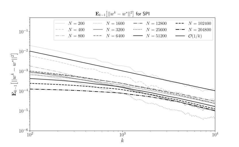
Figure 1. Approximated errors $\mathbf{E}_{k-1}[\|w^{k}-w^{*}\|_{N}^{2}]$ for the SPI method, measured in RMS-norm, for discretizations with varying number of grid points $N$. Statistics were only computed at every $100$ time steps, this is why the plot starts at $k=100$. The $1/k$-convergence is clearly seen by comparing to the uppermost solid black reference line.

In contrast, redoing the same experiment but with the explicit SGD method instead results in Figure 2. We note that except for $N=200$ and $N=400$, the method does not converge at all, likely because as $N$ grows the problem also becomes more stiff. Even when it does converge, the errors are much larger than in Figure 1. Many more steps would be necessary to reach the same accuracy as SPI. Since our implementations are certainly not optimal in any sense, we do not show a comparison of computational times here. They are, however, very similar, meaning that SPI is more efficient than SGD for this problem.

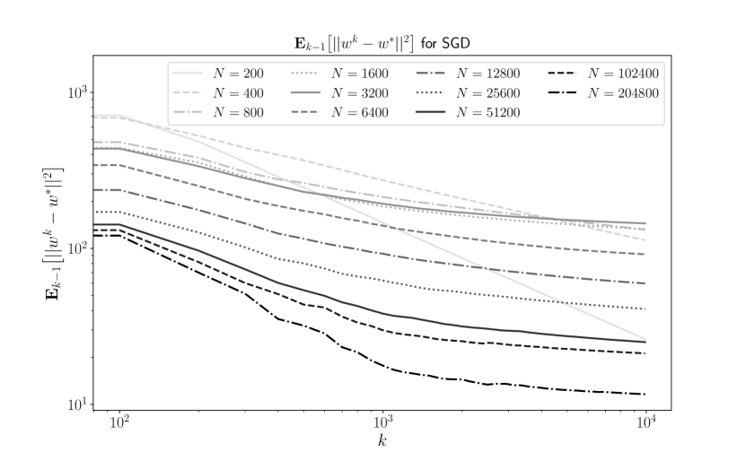
Figure 2. Approximated errors $\mathbf{E}_{k-1}[\|w^{k}-w^{*}\|_{N}^{2}]$ for the SGD method, measured in RMS-norm, for discretizations with varying number of grid points $N$. Statistics were only computed at every $100$ time steps, this is why the plot starts at $k=100$. Except for $N=200$ and $N=400$, the method does not converge at all. Even when it does, the errors are much larger than in Figure 1.

6. Conclusions

We have rigorously proved convergence with an optimal rate for the stochastic proximal iteration method in a general Hilbert space. This improves the analysis situation in two ways. Firstly, by providing an extension of similar results in a finite-dimensional setting to the infinite-dimensional case, as well as extending these to less bounded operators. Secondly, by improving on similar infinite-dimensional results that only achieve convergence, without any error bounds. The latter improvement comes at the cost of stronger assumptions on the cost functional. Global Lipschitz continuity of the gradient is, admittedly, a rather strong assumption. However, as we have demonstrated, this can be replaced by local Lipschitz continuity where the maximal growth of the Lipschitz constant is determined by higher moments of the gradient applied to the minimum. This is a weaker condition. Finally, we have seen that the theoretical results are applicable also in practice, as demonstrated by the numerical results in the previous section.

References

[1]
A. Agarwal, P. L. Bartlett, P. Ravikumar, and M. J. Wainwright.
Information-theoretic lower bounds on the oracle complexity of
stochastic convex optimization.
IEEE Trans. Inform. Theory, 58(5):3235–3249, 2012.
[2]
H. Asi and J. C. Duchi.
Modeling simple structures and geometry for better stochastic
optimization algorithms.
In Kamalika Chaudhuri and Masashi Sugiyama, editors, Proceedings
of the Twenty-Second International Conference on Artificial Intelligence and
Statistics, volume 89 of Proceedings of Machine Learning Research,
pages 2425–2434, Naha, Japan, 16–18 Apr 2019. PMLR.
[3]
H. Asi and J. C. Duchi.
Stochastic (approximate) proximal point methods: convergence,
optimality, and adaptivity.
SIAM J. Optim., 29(3):2257–2290, 2019.
[4]
V. Barbu.
Nonlinear Differential Equations of Monotone Types in
Banach Spaces.
Springer-Verlag, New York, 2010.
[5]
H. H. Bauschke and P. L. Combettes.
Convex analysis and monotone operator theory in Hilbert
spaces.
CMS Books in Mathematics/Ouvrages de Mathématiques de la SMC.
Springer, Cham, second edition, 2017.
[6]
D. P. Bertsekas.
Incremental proximal methods for large scale convex optimization.
Math. Program., 129(2, Ser. B):163–195, 2011.
[7]
P. Bianchi.
Ergodic convergence of a stochastic proximal point algorithm.
SIAM J. Optim., 26(4):2235–2260, 2016.
[8]
P. Bianchi and W. Hachem.
Dynamical behavior of a stochastic forward-backward algorithm using
random monotone operators.
J. Optim. Theory Appl., 171(1):90–120, 2016.
[9]
L. Bottou, F. E. Curtis, and J. Nocedal.
Optimization methods for large-scale machine learning.
SIAM Rev., 60(2):223–311, 2018.
[10]
Z. Brzeźniak, E. Carelli, and A. Prohl.
Finite-element-based discretizations of the incompressible
Navier-Stokes equations with multiplicative random forcing.
IMA J. Numer. Anal., 33(3):771–824, 2013.
[11]
D. S. Clark.
Short proof of a discrete Gronwall inequality.
Discrete Appl. Math., 16(3):279–281, 1987.
[12]
D. Davis and D. Drusvyatskiy.
Stochastic model-based minimization of weakly convex functions.
SIAM J. Optim., 29(1):207–239, 2019.
[13]
J. Eckstein and D. P. Bertsekas.
On the Douglas-Rachford splitting method and the proximal point
algorithm for maximal monotone operators.
Math. Programming, 55(3, Ser. A):293–318, 1992.
[14]
M. Eisenmann.
Methods for the Temporal Approximation of Nonlinear,
Nonautonomous Evolution Equations.
PhD thesis, TU Berlin, 2019.
[15]
M. Eisenmann, M. Kovács, R. Kruse, and S. Larsson.
On a randomized backward Euler method for nonlinear evolution
equations with time-irregular coefficients.
Found. Comput. Math., 19(6):1387–1430, 2019.
[16]
F. Fagan and G. Iyengar.
Unbiased scalable softmax optimization.
ArXiv Preprint, arXiv:1803.08577, 2018.
[17]
W. W. Hager.
Updating the inverse of a matrix.
SIAM Rev., 31(2):221–239, 1989.
[18]
I. Lasiecka and R. Triggiani.
Control theory for partial differential equations: continuous
and approximation theories. I, volume 74 of Encyclopedia of
Mathematics and its Applications.
Cambridge University Press, Cambridge, 2000.
Abstract parabolic systems.
[19]
N. S. Papageorgiou.
Convex integral functionals.
Trans. Amer. Math. Soc., 349(4):1421–1436, 1997.
[20]
N. S. Papageorgiou and P. Winkert.
Applied Nonlinear Functional Analysis. An Introduction.
De Gruyter, Berlin, 2018.
[21]
A. Patrascu and P. Irofti.
Stochastic proximal splitting algorithm for composite minimization.
ArXiv Preprint, arXiv:1912.02039v2, 2020.
[22]
A. Patrascu and I. Necoara.
Nonasymptotic convergence of stochastic proximal point methods for
constrained convex optimization.
J. Mach. Learn. Res., 18(Paper 198):1–42, 2018.
[23]
A. Quarteroni and A. Valli.
Domain decomposition methods for partial differential
equations.
Numerical Mathematics and Scientific Computation. The Clarendon
Press, Oxford University Press, New York, 1999.
Oxford Science Publications.
[24]
M. Raginsky and A. Rakhlin.
Information-based complexity, feedback and dynamics in convex
programming.
IEEE Trans. Inform. Theory, 57(10):7036–7056, 2011.
[25]
R. T. Rockafellar.
On the maximal monotonicity of subdifferential mappings.
Pacific J. Math., 33:209–216, 1970.
[26]
R. T. Rockafellar.
Monotone operators and the proximal point algorithm.
SIAM J. Control Optimization, 14(5):877–898, 1976.
[27]
R. T. Rockafellar and R. J.-B. Wets.
On the interchange of subdifferentiation and conditional expectations
for convex functionals.
Stochastics, 7(3):173–182, 1982.
[28]
L. Rosasco, S. Villa, and B. C. Vũ.
Convergence of stochastic proximal gradient algorithm.
Appl. Math. Optim., 82(3):891–917, 2020.
[29]
E. Ryu and S. Boyd.
Stochastic proximal iteration: A non-asymptotic improvement upon
stochastic gradient descent.
www.math.ucla.edu/eryu/papers/spi.pdf, 2016.
Accessed 20 March 2020.
[30]
E. K. Ryu and W. Yin.
Proximal-proximal-gradient method.
J. Comput. Math., 37(6):778–812, 2019.
[31]
A. Salim, P. Bianchi, and W. Hachem.
Snake: a stochastic proximal gradient algorithm for regularized
problems over large graphs.
IEEE Trans. Automat. Control, 64(5):1832–1847, 2019.
[32]
P. Toulis, E. Airoldi, and J. Rennie.
Statistical analysis of stochastic gradient methods for generalized
linear models.
In Eric P. Xing and Tony Jebara, editors, Proceedings of the
31st International Conference on Machine Learning, volume 32 of Proceedings of Machine Learning Research, pages 667–675, Bejing, China,
22–24 Jun 2014. PMLR.
[33]
P. Toulis and E. M. Airoldi.
Scalable estimation strategies based on stochastic approximations:
classical results and new insights.
Stat. Comput., 25(4):781–795, 2015.
[34]
P. Toulis and E. M. Airoldi.
Asymptotic and finite-sample properties of estimators based on
stochastic gradients.
Ann. Statist., 45(4):1694–1727, 2017.
[35]
P. Toulis, T. Horel, and E. M. Airoldi.
The proximal Robbins–Monro method.
ArXiv Preprint, arXiv:1510.00967v4, 2020.
[36]
P. Toulis, D. Tran, and E. Airoldi.
Towards stability and optimality in stochastic gradient descent.
In Arthur Gretton and Christian C. Robert, editors, Proceedings
of the 19th International Conference on Artificial Intelligence and
Statistics, volume 51 of Proceedings of Machine Learning Research,
pages 1290–1298, Cadiz, Spain, 09–11 May 2016. PMLR.
[37]
D. Tran, P. Toulis, and E. M. Airoldi.
Stochastic gradient descent methods for estimation with large data
sets.
ArXiv Preprint, arXiv:1509.06459, 2015.
[38]
E. Zeidler.
Nonlinear Functional Analysis and its Applications.
II/B.
Springer-Verlag, New York, 1990.
Nonlinear monotone operators.