Two-sided bounds on free energy of directed polymers on strongly recurrent graphs

Abstract

We study the directed polymers in random environment on an infinite graph $G=(V,E)$ on which the underlying random walk satisfies sub-Gaussian heat kernel bounds with spectral dimension $d_{s}$ strictly less than two. Our goal in this paper is to show (i) the existence and the coincidence of the quenched and the annealed free energy $F_{q}(\beta)$, $F_{a}(\beta)$ and (ii) that $F_{a}(\beta)-F_{q}(\beta)$ is comparable to $\beta^{\frac{4}{2-d_{s}}}$ for small inverse temperature $\beta$.

AMS 2010 Subject Classification: Primary 82D60. Secondary 82C44.

Key words: directed polymers in random environment, phase transition, fractal graph, free energy, strongly recurrent graphs.

For a probability space $(\Omega,{\cal F},P)$, we denote by $P[X]$ the expectation of random variable $X$ with respect to $P$. Let $\mathbb{N}_{0}=\{0,1,2,\cdots\}$, $\mathbb{N}=\{1,2,3,\cdots\}$, and $\mathbb{Z}=\{0,\pm 1,\pm 2,\cdots\}$. Let $C_{x_{1},\cdots,x_{p}}$ or $C(x_{1},\cdots,x_{p})$ be a non-random constant which depends only on the parameters $x_{1},\cdots,x_{p}$.

1 Introduction

1.1 The model.

The directed polymers in random environment (DPRE) was introduced by Henley and Huse [23] in the physics literature to analyze an influence of random media to the shape of polymer chains. Later on, Imbrie-Spencer and Bolthausen succeeded to treat DPRE mathematically [24, 7]. Then, a lot of progress has been achieved by many authors [2, 10, 17, 16, 15]. In particular, it is known that the phase transition of delocalization-localization of polymer chain is characterized by the free energy[16]. The reader may refer the survey text [14].

In the most studied model, polymer chain and random media are represented by a path of random walk on graph $\mathbb{Z}^{d}$ and time-space i.i.d. random variables $\omega$ respectively, and their interaction is described in terms of Gibbs measure with Hamiltonian $H(\omega,S)$. In this paper, we consider the model on a general infinite graph $G=(V,E)$ with bounded degree and replace the underlying walk by a reversible random walk $S$.

To formulate our model, we introduce a framework of a graph $G=(V,E)$ and a random walk $S=\{S_{n}\}_{n=0}^{\infty}$ with suitable conditions as in [5].

Graph and random walk Let $G=(V,E)$ be an infinite graph where $V$ is the set of vertices with countably infinite elements and $E$ is the set of undirected edges. Let $0\in V$ be the distinguished vertex called the origin. We assume that graph does not have multiple edges. Then, each edge is identified as a pair of vertices $\left\langle x,y\right\rangle$ and we denote by $N(x)=\left\{y\in V:\text{There exists $e\in E$ s.t.~{}}e=\left\langle y,x\right\rangle\right\}$.

We assume that

graph $$G$$ is connected, (1.1)

that is, for any $x,y\in V$, there exist an $n\in\mathbb{N}$ and a sequence of $x_{0},x_{1},\cdots,x_{n}\in V$ such that $x_{0}=x$, $x_{n}=y$ and $\left\langle x_{i-1},x_{i}\right\rangle\in E$ for each $i=1,\cdots,n$.

Also, we introduce the weight $\{\mu_{xy}\}_{x,y\in V}$ on graph $G$ such that

1. $\mu_{xy}=\mu_{yx}$.

2. $\mu_{xy}\geq 0$ for any $x,y\in V$.

3. $\mu_{xy}>0$ if and only if $\left\langle x,y\right\rangle\in E$.

We consider a random walk $S$ on weighted graph $G$ with transition probability given by

$$p_{x,y}=P_{S}(S_{n+1}=y|S_{n}=x)=\frac{\mu_{xy}}{\mu_{x}},\quad y\in N(x),$$

where $\mu_{x}=\displaystyle\sum_{y\in N(x)}\mu_{xy}$ and we denote by $(\Omega_{S},\mathcal{G}_{S},P_{S})$ the probability space on which $S$ is defined. In particular, $P_{S}^{x}$ denotes the law of $S$ starting from $x\in V$, and also by $P_{S}=P_{S}^{0}$ for simplicity.

We remark that a random walk $S$ is reversible since

$$\mu_{x}p_{x,y}=\mu_{y}p_{y,x}.$$

Throughout the paper, we assume the “bounded weights” condition: There exists a constant $C_{\mu}$ such that

$$C_{\mu}^{-1}\leq\mu_{xy}\leq C_{\mu}$$ (BW)

for any $x,y\in V$ with $\langle x,y\rangle\in E$.

Random media Let $\{\omega(n,x):n\in\mathbb{N},x\in V\}$ be i.i.d. $\mathbb{R}$-valued random variables which are independent of $S$ and defined on the probability space $(\Omega,\mathcal{F},Q)$. In this paper, we assume

$$Q[\omega(n,x)]=0,\quad\text{and }\quad Q\left[\exp\left(\beta\omega(n,x)\right)\right]=:e^{\lambda(\beta)}<\infty\text{ for all }\beta\in\mathbb{R}.$$ (1.2)

For each $n\in\mathbb{N}$, $z\in V$, let $\theta_{n,x}:\Omega\to\Omega$ be a time-space shift of random media:

$$\theta_{n,z}\circ\omega(m,y)=\omega(m+n,y+z)$$

and we define $\theta_{n,z}\circ f(\omega):=f(\theta_{n,z}\circ\omega)$ for a measurable function $f:\Omega\to\mathbb{R}$.

Then, Hamiltonian is defined by

$$H_{n}(S,\omega)=\sum_{i=1}^{n}\omega(i,S_{i})$$

and the polymer measure is given by

$$P_{n,x}^{\beta}(dS)=\frac{1}{Z_{n,\beta}^{x}}\exp\left(\beta H_{n}(S,\omega)\right)P_{S}^{x}(dS)$$

where

$$Z^{x}_{n,\beta}:=Z_{n}^{x}=P_{S}^{x}\left[\exp\left(\beta H_{n}(S,\omega)\right)\right]$$

is the normalizing constant called a partition function.

Then, the argument in [17, Theorem 3.2] assure the existence of a critical point $\beta_{1}\in[0,\infty]$ such that

$$Q(W_{\infty,\beta}^{x}>0)=\begin{cases}1\ (\text{weak disorder})\quad&\beta\in\{0\}\cup[0,\beta_{1})\\ 0\ (\text{strong disorder})\quad&\beta\in(\beta_{1},\infty).\end{cases}$$

One then defines the free energy of the systems.

Proposition 1.1.

Assume that for each $x\in V$,

$$\varlimsup_{n\to\infty}\frac{1}{n}\log\tilde{V}(x,n)=0,$$ (subExp)

where $\tilde{V}(x,n)$ is the number elements in the ball centered at $x$ with radius $n$.

Then, for any $x\in V$, the following limit exists and is constant $Q$-a.s.:

$$F_{q,x}(\beta) =\lim_{n\to\infty}\frac{1}{n}\log Z_{n,\beta}^{x}=\lim_{n\to\infty}\frac{1}{n}Q[\log Z_{n}^{x}(\beta)]$$

$$F_{a}(\beta) =\lim_{n\to\infty}\frac{1}{n}\log Q[Z_{n,\beta}^{x}]=\lambda(\beta).$$

In particular, $F_{q,x}(\beta)$ is constant in $x\in V$ and we denote by $F_{q}(\beta)=F_{q,x}(\beta)$ $(x\in V)$.

$F_{q,x}(\beta)$ and $F_{a}(\beta)$ are called the quenched free energy and the annealed free energy of the systems, respectively.

Remark 1.2.

Jensen’s inequality implies that

$$\frac{1}{n}Q[\log Z_{n,\beta}^{x}]\leq\frac{1}{n}\log Q[Z_{n,\beta}^{x}]=\lambda(\beta)$$

and $F_{q}(\beta)\leq\lambda(\beta)=:F_{a}(\beta)$. The same argument as in [17, Theorem 3.2] assures the existence of critical point $\beta_{2}\in[0,\infty]$ such that

$$F_{q}(\beta)-F_{a}(\beta)\begin{cases}=0\quad&\beta\in[0,\beta_{2}]\\ <0\ (\text{very strong disorder})\quad&\beta\in(\beta_{2},\infty).\end{cases}$$

Our main result gives an asymptotic order of $F_{q}(\beta)-F_{a}(\beta)$, where the detail of assumptions is discussed in subsection 1.2:

Theorem 1.3.

1. Suppose that the underlying random walk $S$ satisfies upper heat kernel condition (UHK) with $d_{s}<2$ and (VG). Then, there exist constants $C_{1}>0$ and $\beta_{0}>0$ such that for any $\beta\in[0,\beta_{0})$

   $$F_{q}(\beta)-F_{a}(\beta)\leq-C_{2}\beta^{\frac{4}{2-d_{s}}}.$$

   In particular, $\beta_{1}=\beta_{2}=0$.

2. In addition, we suppose that the underlying random walk $S$ satisfies lower heat kernel condition (LHK) with $d_{s}<2$. Then, there exists a constant $C_{2}>0$ such that for any $\beta\in[0,\beta_{0})$

   $$-C_{2}\beta^{\frac{4}{2-d_{s}}}\leq F_{q}(\beta)-F_{a}(\beta).$$

For DPRE in $1+1$ ($d_{f}=1$ and $d_{w}=2$), the same upper bound (and lower bound for Gaussian environment) was obtained by H. Lacoin [25] and the same lower bound was obtained by K.S. Alexander and G. Yildirim [3].

Remark 1.4.

Cosco, Seroussi, and Zeitouni study the DPRE on infinite graphs independently [18]. They discuss the critical points of phase transitions for large classes of graphs. They also obtain an upper bound of asymptotics of free energy under a similar set of conditions independently.

1.2 Heat kernel estimate

In this subsection, we review some selected facts on the random walk on graphs $G=(V,E)$.

Let $B(x,n)=\{y\in V:d(x,y)\leq n\}$ be a ball centered at $x$ with radius $n$, where $d(x,y)$ is a graph distance of $x,y\in V$, that is $d(x,y)=\inf\{n\geq 0:\text{There exists a sequence $\{x_{i}\}_{i=0}^{n}\subset V$, $x=x_{0},x_{1},\cdots,x_{n}=y$ such that $\langle x_{i-1},x_{i}\rangle\in E$}\}$. For $x\in V$ and a nonempty subset $A,B\subset V$, we denote the distance between $x$ and $A$ by

$$d(x,A):=\inf\{d(x,y):y\in A\}$$

and the distance between $A$ and $B$ by

$$d(A,B)=\inf\{d(x,y):x\in A,y\in B\}.$$

Here, we list some properties of graphs and random walk. Let $d_{f}>0$ and $d_{w}>1$.

• (Upper heat kernel estimate) There exist constants $c_{1},c_{2}>0$ such that for $n\geq 0$ and $x,y\in V$ with $d(x,y)\leq n$

  $$p_{n}(x,y)\leq\frac{c_{1}}{(n\vee 1)^{d_{f}/d_{w}}}\exp\left(-c_{2}\left(\frac{d(x,y)^{d_{w}}}{n\vee 1}\right)^{\frac{1}{d_{w}-1}}\right).$$ (UHK)

• (Lower heat kernel estimate) There exist constants $c_{3},c_{4}>0$ such that for $n\geq 0$ and $x,y\in V$ with $d(x,y)\leq n$

  $$\frac{c_{3}}{(n\vee 1)^{d_{f}/d_{w}}}\exp\left(-c_{4}\left(\frac{d(x,y)^{d_{w}}}{n\vee 1}\right)^{\frac{1}{d_{w}-1}}\right)\leq p_{n}(x,y)+p_{n+1}(x,y)$$ (LHK)

• (Bounded geometry) The degree is bounded, that is

  $$\sup_{x\in V}|N(x)|<\infty$$ (BG)

• (Volume growth) There exists a non-random constant $C_{V}>0$ s.t.

  $$C_{V}^{-1}n^{d_{f}}\leq V(x,n)\leq C_{V}n^{d_{f}}\quad\text{for $x\in V$ and $n\geq 1$},$$ (VG)

  where $V(x,n)$ be the volume growth function:

  $$V(x,n)=\mu(B(x,n))=\sum_{y\in B(x,n)}\mu_{y}\quad\text{for }x\in V,n\geq 1.$$

When (UHK) and (LHK) are satisfied, $d_{w}>1$ is called the walk dimension of $S$ and $d_{s}:=2d_{f}/d_{w}$ is called the spectral dimension of $S$ [5, Definition 4.14].

We say the weighted graph is strongly recurrent if the random walk $S$ satisfies (UHK) and (LHK) with $d_{f}<d_{w}$, or equivalently, $d_{s}=2d_{f}/d_{w}<2$. [6, Section 1.1]

Remark 1.5.

• (UHK) and (LHK) imply (BW), (BG), (VG) [5, Lemma 4.17].

• (BW) and (VG) imply that there exists a non-random constant $C_{V}^{\prime}>0$ s.t.

  $${C_{V}^{\prime}}^{-1}n^{d_{f}}\leq\tilde{V}(x,n)\leq C_{V}^{\prime}n^{d_{f}}\quad\text{for }x\in V,n\geq 1,$$ (VG’)

  where $\tilde{V}(x,n)=\sharp B(x,n)$ is the number of elements in the ball $B(x,n)$.

Lemma 1.6.

[5, Lemma 4.21] We assume (UHK). Then, there exist constants $c_{5},c_{6}$ such that for $t\geq 1$,

$$P_{x}\left(S_{n}\not\in B(x,tn^{\frac{1}{d_{w}}})\right) \leq c_{5}\exp\left(-c_{6}t^{\frac{d_{w}}{d_{w}-1}}\right)$$ (1.3)

$$P_{x}\left(\tau(x,2tn^{\frac{1}{d_{w}}})<n\right) \leq 2c_{5}\exp\left(-c_{6}t^{\frac{d_{w}}{d_{w}-1}}\right),$$ (1.4)

where $\tau(x,r)=\inf\{n\geq 0:S_{n}\not\in B(x,r)\}$ for $r\geq 1$.

1.2.1 Example of strongly recurrent graphs

Here, we will consider random walk on the Sierpinski gasket graph as an example of strongly recurrent graphs. See [5, Section2.9].

Let $O=(0,0)$, $a_{0}=(1,0)$, $b_{0}=({\frac{1}{2}},\frac{\sqrt{3}}{{2}})$. Let $G_{0}$ be the graph which consists of the vertices $O$, $a_{0}$, and $b_{0}$ and the edges $\langle O,a_{0}\rangle$, $\langle O,b_{0}\rangle$, and $\langle a_{0},b_{0}\rangle$. Then, we consider the sequence of graphs $\{G_{n}\}_{n=0}^{\infty}$ defined by

$$G_{n+1}=G_{n}\cup(G_{n}+2^{n}a_{0})\cup(G_{n}+2^{n}b_{0}),$$

where $A+a=\{x+a:x\in A\}$. Then, the graph $\displaystyle G=\bigcup_{n=0}^{\infty}G_{n}$ is the Sierpinski gasket graph.

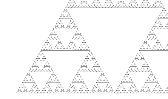
Figure 1: Sierpinski gasket graph

When we consider a simple random walk $S_{\textrm{SG}}$ on $G$, it is known that $S_{\textrm{SG}}$ satisfies (UHK) and (LHK) with $d_{f}=\frac{\log 3}{\log 2}$, $d_{w}=\frac{\log 5}{\log 2}$ and hence $d_{s}=\frac{\log 9}{\log 5}<1$ [5, Corollary 6.11].

1.3 Some remarks and Comments

For DPRE in $1+1$, one of authors obtained a sharper asymptotics as follows [28]. Suppose we assume (1.2) and $Q[\omega(n,x)^{2}]=1$ with a certain technical condition on $\omega$, then

$$\lim_{\beta\to 0}\frac{F_{q}(\beta)-F_{a}(\beta)}{\beta^{4}}=\lim_{T\to\infty}\frac{1}{T}\mathcal{P}[\log\mathcal{Z}_{T}]$$ (1.5)

with $\mathcal{Z}_{T}=\displaystyle\int_{\mathbb{R}}\mathcal{Z}(T,x)dx$, where $\mathcal{Z}(t,x)$ is a solution to a stochastic heat equation

$$\partial_{t}\mathcal{Z}=\frac{1}{2}\Delta\mathcal{Z}+\sqrt{2}\mathcal{Z}\dot{\mathcal{W}},\quad\lim_{t\to 0}\mathcal{Z}(t,x)dx=\delta(dx),$$

where $\mathcal{W}$ is a time-space white noise on $[0,\infty)\times\mathbb{R}$.

To explain the rough idea of (1.5), we need the following theorem obtained by T. Alberts, K. Khanin, and J. Quastel[1, Theorem 2.1]:

Theorem A.

Suppose (1.2) and $Q[\omega(n,x)^{2}]=1$. Then we have

$$\frac{Z_{Tn,\beta_{n}}^{0}}{Q\left[Z_{Tn,\beta_{n}}^{0}\right]}\Rightarrow\mathcal{Z}_{T}$$

where $\beta_{n}=n^{-\frac{1}{4}}$.

Then, (1.5) implies roughly that

$$(LHS)=\lim_{n\to\infty}\frac{1}{\beta_{n}^{4}}\lim_{T\to\infty}\frac{1}{Tn}Q\left[\log\frac{Z_{Tn,\beta_{n}}^{0}}{Q\left[Z_{Tn,\beta_{n}}^{0}\right]}\right]=\lim_{T\to\infty}\lim_{n\to\infty}\frac{1}{T}Q\left[\log\frac{Z_{Tn,\beta_{n}}^{0}}{Q\left[Z_{Tn,\beta_{n}}^{0}\right]}\right]=(RHS),$$

that is (1.5) means the interchangeability of two limits in $n$ and $T$. In several discrete disordered systems, it is known that such interchangeability of limits holds [9, 11, 12]

Thus, we have the following conjectures.

Conjecture A.

Suppose the underlying random walk satisfies the local limit theorem in the sense discussed in [19]. Then, we have for each $T>0$

$$\frac{Z^{0}_{Tn,\beta_{n}}}{Q\left[Z_{Tn,\beta_{n}}^{0}\right]}\Rightarrow\mathcal{Z}_{T},$$

with $\beta_{n}=n^{-\frac{d_{w}-d_{f}}{2d_{w}}}$, $\mathcal{Z}_{T}=\int_{\bar{V}}\mathcal{Z}_{T,x}\mu(dx)$, where $\mathcal{Z}_{t,x}$ satisfies the

$$\mathcal{Z}_{t,x}=p_{t}(x)+\hat{\beta}\int_{0}^{t}\int_{\bar{V}}\left(\int_{\bar{V}}p_{t-s}(x-z)\mathcal{Z}_{s,z-y}\mu(dz)\right)\mathcal{W}(ds,dy),$$ (1.6)

where $\hat{\beta}$ is a constant depends on underlying random walk and $p_{t}(x)$ is a heat kernel of Brownian motion in fractal graph and $\mathcal{W}$ is a white noise on $(\bar{V},\mu)$.

Remark 1.7.

Simple random walk on Sierpinski gasket graph satisfies local limit theorem[19].

Remark 1.8.

In [22, 21], SPDE on measure space equipped with gradient and divergence are discussed and they prove the existence and uniqueness of solutions.

Conjecture B.

Under the assumption in Conjecture A, we have that

$$\lim_{\beta\to 0}\beta^{-\frac{4}{2-d_{s}}}(F_{q}(\beta)-F_{a}(\beta))=\lim_{T\to\infty}\frac{1}{T}\mathcal{P}\left[\log\mathcal{Z}_{T}\right].$$

2 The existence of the free energy

In this section, we prove Proposition 1.1 and we assume (subExp) and (BW).

In [15], the existence of the limit $\displaystyle\lim_{n\to\infty}\frac{1}{n}Q[\log Z_{n,\beta}^{x}]$ follows from superadditivity of $\{Q[\log Z_{n,\beta}^{x}]\}_{n=1}^{\infty}$, but we should remark that $\{Q[\log Z_{n,\beta}^{x}]\}_{n=1}^{\infty}$ is not superadditive in our case due to loss of the shift invariance of the underlying random walk.

Letting $Z^{x,y}_{n,\beta}$ be the point to point partition function

$$Z^{x,y}_{n,\beta}=Z_{n}^{x,y}:=P_{x}\left[\exp\left(\beta\sum_{i=1}^{n}\omega(i,S_{i})\right):S_{n}=y\right],$$

then $\{Q[\log Z^{x,x}_{n}]\}_{n=1}^{\infty}$ is superadditive and hence the limit $\lim_{n\to\infty}\frac{1}{n}Q[\log Z^{x,x}_{n}]=\sup_{n\geq 1}\frac{1}{n}Q[\log Z^{x,x}_{n}]$ exists.

Proof of Proposition 1.1.

Theorem 6.1 [27] combined with [15, Proposition 1.5] gives the concentration inequality for $\log Z_{n}^{x,y}$ and $\log Z_{n}^{x}$: There exists a constant $K>0$ such that for any $n\geq 1$, $t\in(-1,1)$, $\delta>0$, and $x,y\in V$

$$Q\left[\exp\left(t(\log Z^{x}_{n}-Q[\log Z^{x}_{n}])\right)\right] \leq\exp\left(\frac{nKt^{2}}{1-|t|}\right)$$ (2.1)

and

$$Q\left(\left|\log Z_{n}^{x}-Q[\log Z_{n}^{x}]\right|>n\delta\right) \leq\exp\left(-n\left(\sqrt{\delta+K}-\sqrt{K}\right)^{2}\right),$$

and the same inequality holds even if $Z_{n}^{x}$ is replaced by $Z_{n}^{x,y}$.

Thus, it is enough to show the convergence of $\frac{1}{n}Q[\log Z_{n}^{x}]$ and independence of $x\in V$. We will show that

$$\lim_{n\to\infty}\frac{1}{n}Q[\log Z_{n}^{x}]=\lim_{n\to\infty}\frac{1}{n}Q[\log Z^{x,x}_{n}]$$

by the same argument as in [13, Proposition 2.4]: $Z_{n}^{x}\geq Z^{x}_{n,x}$ is trivial so that

$$\lim_{n\to\infty}\frac{1}{n}Q[\log Z^{x,x}_{n}]\leq\varliminf_{n\to\infty}\frac{1}{n}Q[\log Z^{x}_{n}].$$

Also, $Q[\log Z^{x,x}_{2n}]\geq Q[\log Z_{n}^{x,y}]+Q[\log Z_{n}^{y,x}]$ with (BW) implies that there exists a constant $c>0$ such that for any $x,y\in V$

$$Q[\log Z^{x,x}_{2n}]\geq 2Q[\log Z_{n}^{x,y}]-c.$$ (2.2)

On the other hand, we have that for any $0<t<1$

$$\frac{1}{n}Q[\log Z^{x}_{n}] \leq\frac{1}{tn}\log Q\left[\left(Z_{n}^{x}\right)^{t}\right]\hskip 100.00015pt(\text{Jensen's inequality})$$

$$\leq\frac{1}{tn}\log Q\left[\sum_{y\in V}\left(Z_{n,y}^{x}\right)^{t}\right]$$

$$=\frac{1}{tn}\log\left(\sum_{y\in V}Q\left[\exp\left(t\left(\log Z_{n}^{x,y}-Q[\log Z_{n}^{x,y}]\right)\right)\right]\exp\left(tQ[\log Z_{n}^{x,y}]\right)\right)$$

$$\leq\frac{1}{tn}\log Q\left[\sum_{y\in V}\exp\left(t\left(\log Z_{n}^{x,y}-Q[\log Z^{x,y}_{n}]\right)\right)\right]+\frac{1}{2n}Q[\log Z_{2n}^{x,x}]+\frac{c}{2nt}$$

$$\leq\frac{1}{tn}\left(\log\tilde{V}(x,n)+\frac{nKt^{2}}{1-t}\right)+\frac{1}{2n}Q[\log Z_{2n}^{x,x}]+\frac{c}{2nt},$$ (2.3)

where we used Jensen’s inequality in the first line, the fact $(a+b)^{\theta}\leq a^{\theta}+b^{\theta}$ for $a,b\geq 0$ and $\theta\in(0,1)$ in the second line, (2.2) in the fourth line, and (2.1) in the last line.

Taking $n\to\infty$ and then $t\to 0$, we obtain from (subExp) that

$$\varlimsup_{n\to\infty}\frac{1}{n}Q[\log Z_{n}^{x}]\leq\lim_{n\to\infty}\frac{1}{2n}Q[\log Z_{2n}^{x,x}]$$

and thus $\lim_{n\to\infty}\frac{1}{n}Q[\log Z_{n}^{x}]$ exists. The independence of $x$ for $F_{q,x}(\beta)$ follows by $Q[\log Z^{x}_{n+d(x,y)}]\geq Q[\log Z^{y}_{n}]$.

∎

3 Upper bound

In this section, we prove Theorem 1.3 (1). Throughout this section, we assume (BW), (VG) (which imply (VG’)), (UHK).

We will prove the upper bound by the coarse graining scheme and change of measure method used in several polymer models [4, 8, 9, 25, 20, 30].

3.1 Coarse graining and change of measure

We define $W_{n,\beta}^{x}=Z_{n,\beta}^{x}/Q[Z_{n,\beta}^{x}]=P_{S}^{x}\left[e_{n}\right]$ where

$$e_{n}=e_{n}(\beta,\omega,S):=\exp\left(\beta H_{n}(S)-n\lambda(\beta)\right)$$ (3.1)

and we denote by $\{\mathcal{F}_{n}:n\geq 0\}$ the filtration generated by $\omega(n,x)$: $\mathcal{F}_{0}=\{\Omega,\emptyset\}$ and $\mathcal{F}_{n}=\sigma[\omega(i,x):1\leq i\leq n,x\in V]$ for $n\geq 1$.

We remark from Proposition 1.1 that

$$F_{q}(\beta)-F_{a}(\beta)=\lim_{n\to\infty}\frac{1}{n}Q[\log W_{n}^{0}(\beta)]=\lim_{N\to\infty}\frac{1}{nN}Q[\log W_{nN}^{0}(\beta)].$$ (3.2)

Therefore, we will estimate the RHS in (3.2) in the proof.

For small $\beta>0$, let $n$ be the smallest integer bigger than $h_{V}(\beta)$, where $h_{V}$ is a decreasing function on $(0,{\beta_{0}})$ with $\lim_{\beta\to+0}h_{V}(0)=\infty$ and given explicitly later. First, we consider a covering of graph by balls with radius $n_{w}=n^{\frac{1}{d_{w}}}$. From Vitali’s covering lemma, we can find a set of verticies $I^{(n)}=\{y_{i}^{(n)}\}_{i\in\mathbb{N}}$ such that

1. $B(y_{i}^{(n)},n_{w})\cap B(y_{j}^{(n)},n_{w})=\emptyset$ for $i\not=j$.

2. $\displaystyle\bigcup_{i}B(y_{i}^{(n)},5n_{w})=V$.

Denoting by $\mathcal{N}_{i}^{(n)}(R)$ the elements in $I^{(n)}$ which lie in the ball $B(y_{i}^{(n)},Rn_{w})$ for $R\geq 1$, we have

$$\bigcup_{j\in\mathcal{N}_{i}^{(n)}}B(y_{j}^{(n)},n_{w})\subset B(y_{i}^{(n)},(R+1)n_{w})$$

and hence (VG’) implies that there exists a constant $C_{C}>0$ such that

$$\sharp\mathcal{N}_{i}^{(n)}(R)\leq C_{C}R^{d_{f}}$$ (3.3)

for any $n\geq 1$ and $y_{i}^{(n)}\in I^{(n)}$.

Jensen’s inequality implies that for each $0<\theta<1$

$$\frac{1}{nN}Q[\log W_{nN}^{0}(\beta)]\leq\frac{1}{\theta nN}\log Q\left[W_{nN}^{0}(\beta)^{\theta}\right].$$

We will prove that there exists an $m>0$ such that

$$Q\left[W_{nN}^{0}(\beta)^{\theta}\right]\leq e^{-mN}$$ (3.4)

so that

$$\varlimsup_{n\to\infty}h_{V}(\beta)\left(F_{q}(\beta)-F_{a}(\beta)\right)\leq-\frac{m}{\theta}.$$

To estimate $W_{nN}^{0}(\beta)^{\theta}$, we focus on the balls which the underlying random walk passes through in each $m=n,2n,3,\cdots,nN$:

$$W_{nN}^{0}(\beta) =P_{0}\left[\exp\left(\beta H_{nN}(S,\omega)-nN\lambda(\beta)\right)\right]$$

$$\leq\sum_{z_{1},\cdots,z_{N}\in I^{(n)}}P_{0}\left[\exp\left(\beta H_{nN}(S,\omega)-nN\lambda(\beta)\right):S_{in}\in B(z_{i},5n_{w}),i=1,\cdots,N\right].$$

Therefore, we have that

$$Q\left[W_{nN}^{0}(\beta)^{\theta}\right] \leq\sum_{z_{1},\cdots,z_{N}\in I^{(n)}}Q\left[P_{0}\left[\exp\left(\beta H_{nN}(S,\omega)-nN\lambda(\beta)\right):S_{in}\in B(z_{i},5n_{w}),i=1,\cdots,N\right]^{\theta}\right],$$ (3.5)

where we used the fact $(a+b)^{\theta}\leq a^{\theta}+b^{\theta}$ for $a,b\geq 0$ and $\theta\in(0,1)$. For simplicity of notation, we denote by

$$W_{nN}(Z)=P_{0}\left[\exp\left(\beta H_{nN}(S,\omega)-nN\lambda(\beta)\right):S_{in}\in B(z_{i},5n_{w}),i=1,\cdots,N\right].$$

We will take $h_{V}(\beta)=C_{1}\beta^{-\frac{4}{2-d_{s}}}$, where $C_{1}>0$ will be chosen large later. Then, we have that

$$C_{1}\beta^{-\frac{4}{2-d_{s}}}\leq n<C_{1}\beta^{-\frac{4}{2-d_{s}}}+1$$ (3.6)

For each $Z=(z_{1},\cdots,z_{N})\in\left(I^{(n)}\right)^{N}$, we introduce a new probability measure which has a Radon-Nikodym derivative

$$\frac{dQ_{Z}}{dQ} =\exp\left(-\sum_{(l,x)\in J_{Z}}\left(\delta_{n}\omega(l,x)-\lambda(-\delta_{n})\right)\right)$$

$$=\prod_{i=0}^{N-1}\exp\left(-\sum_{(l,x)\in J_{i,z_{i}}}\left(\delta_{n}\omega(l,x)-\lambda(-\delta_{n})\right)\right),$$

where

$$J_{Z}=\left\{(in+k,x)\in\mathbb{N}\times V:i=0,\cdots,N-1,k=1,\cdots,n,x\in B(z_{i-1},C_{2}n_{w})\right\}$$

$$J_{i,z_{i}}=\{(in+k,x)\in\mathbb{N}\times V:k=1,\cdots,n,x\in B(z_{i-1},C_{2}n_{w})\}$$

with $z_{0}=0$, $C_{2}$ will be chosen large later, and $\delta_{n}=(C_{V}^{\prime}n(C_{2}n_{w})^{d_{f}})^{-\frac{1}{2}}$.

Then, Hölder’s inequality yields that

$$Q\left[P_{0}\left[e_{nN}:S_{in}\in B(z_{i},5n_{w}),i=1,\cdots,N\right]^{\theta}\right]$$

$$=Q_{Z}\left[\frac{dQ}{dQ_{Z}}P_{0}\left[e_{nN}:S_{in}\in B(z_{i},5n_{w}),i=1,\cdots,N\right]^{\theta}\right]$$

$$\leq Q_{Z}\left[\left(\frac{dQ}{dQ_{Z}}\right)^{\frac{1}{1-\theta}}\right]^{1-\theta}Q_{Z}\left[P_{0}\left[e_{nN}:S_{in}\in B(z_{i},5n_{w}),i=1,\cdots,N\right]\right]^{\theta}.$$ (3.7)

Set $\theta=\frac{1}{2}$. Then, we know that

$$Q_{Z}\left[\left(\frac{dQ}{dQ_{Z}}\right)^{2}\right] =Q\left[\exp\left(\sum_{(l,x)\in J_{Z}}\left(\delta_{n}\omega(l,x)+\lambda(-\delta_{n})\right)\right)\right]$$

$$=\exp\left(\sum_{(l,x)\in J_{Z}}(\lambda(\delta_{n})+\lambda(-\delta_{n}))\right)$$

$$=\exp\left(n\sum_{i=0}^{N-1}\tilde{V}(z_{i},C_{2}n_{w})(\lambda(\delta_{n})+\lambda(-\delta_{n}))\right)$$

$$\leq\exp\left(NC_{V}^{\prime}C_{2}^{d_{f}}nn_{w}^{d_{f}}(\lambda(\delta_{n})+\lambda(-\delta_{n}))\right)$$

$$\leq\exp\left(NC_{3}C_{V}^{\prime}C_{2}^{d_{f}}nn_{w}^{d_{f}}\delta_{n}^{2}\right)$$

$$\leq e^{C_{3}N},$$ (3.8)

where we have used $\lambda(\beta)+\lambda(-\beta)\leq C_{3}\beta^{2}$ for small $\beta>0$ with some constant $C_{3}>0$.

Markov property of $S$ implies that

$$Q_{Z}\left[P_{0}\left[e_{nN}:S_{in}\in B(z_{i},n_{w}),i=1,\cdots,N\right]^{\frac{1}{2}}\right]$$

$$\leq P_{0}\left[Q_{Z}\left[e_{nN}\right]:S_{in}\in B(z_{i},5n_{w}),i=1,\cdots,N\right]^{\frac{1}{2}}$$

$$\leq\prod_{i=0}^{N-1}\max_{x\in B(z_{i},5n_{w})}P_{x}\left[Q\left[\exp\left(-\sum_{l=1}^{n}\sum_{x\in B(z_{i},C_{4}n_{w})}\delta_{n}\omega(l,x)-\lambda(-\delta_{n})\right)e_{n}\right]:S_{n}\in B(z_{i+1},5n_{w})\right]^{\frac{1}{2}}$$

$$=\prod_{i=0}^{N-1}\max_{x\in B(z_{i},5n_{w})}P_{x}\left[\exp\left((\lambda(\beta-\delta_{n})-\lambda(\beta)-\lambda(-\beta))\sharp\{1\leq l\leq n:S_{l}\in B(z_{i},C_{2}n_{w})\}\right):S_{n}\in B(z_{i+1},5n_{w})\right]^{\frac{1}{2}}$$

$$\leq\prod_{i=0}^{N-1}\max_{x\in B(z_{i},5n_{w})}P_{x}\left[\exp\left(-C_{4}\beta\delta_{n}\sharp\{1\leq l\leq n:S_{l}\in B(z_{i},C_{2}n_{w})\}\right):S_{n}\in B(z_{i+1},5n_{w})\right]^{\frac{1}{2}},$$ (3.9)

where we have used $\lambda(\beta-\delta_{n})-\lambda(\beta)-\lambda(-\beta)\leq-C\beta\delta_{n}$ for small $\beta>0$ with some constant $C_{4}>0$.

Putting together (3.5), (3.7), (3.8), and (3.9), we get

$$Q\left[W_{nN}^{0}(\beta)^{\frac{1}{2}}\right]$$

$$\leq e^{\frac{C_{3}}{2}N}\left(\sup_{y\in I^{(n)}}\sum_{z\in I^{(n)}}\max_{x\in B(y,5n_{w})}P_{x}\left[\exp\left(-C_{4}\beta\delta_{n}\sharp\{1\leq l\leq n:S_{l}\in B(y,C_{2}n_{w})\}\right):S_{n}\in B(z,5n_{w})\right]^{\frac{1}{2}}\right)^{N}.$$

Thus, (3.4) follows when we show that for any $\varepsilon>0$, there exists $C_{1}>0$, $C_{2}>0$ such that

$$\sup_{y\in I^{(n)}}\sum_{z\in I^{(n)}}\max_{x\in B(y,5n_{w})}P_{x}\left[\exp\left(-C_{4}\beta\delta_{n}\sharp\{1\leq l\leq n:S_{l}\in B(y,C_{2}n_{w})\}\right):S_{n}\in B(z,5n_{w})\right]^{\frac{1}{2}}<\varepsilon.$$

For $y\in I^{(n)}$ and $R\in\mathbb{N}$, we consider

$$J_{y,R,1}^{(n)} =\{z\in I^{(n)}:d(B(y,5n_{w}),B(z,5n_{w}))\geq Rn_{w}\},$$

$$J_{y,R,2}^{(n)} =\{z\in I^{(n)}:d(B(y,5n_{w}),B(z,5n_{w}))<Rn_{w}\}.$$

Then, we obtain from (UHK) that for $x\in B(y,5n_{w})$

$$P_{x}(S_{n}\in B(z,5n_{w})) \leq\sum_{u\in B(z,5n_{w})}\frac{c_{1}}{n^{\frac{d_{f}}{d_{w}}}}\exp\left(-c_{2}\left(\frac{d(x,u)^{d_{w}}}{n}\right)^{\frac{1}{d_{w}-1}}\right)$$

$$\leq\tilde{V}(z,5n_{w})\frac{c_{1}}{n^{\frac{d_{f}}{d_{w}}}}\exp\left(-c_{2}\left(\frac{d(B(y,5n_{w}),B(z,5n_{w}))^{d_{w}}}{n}\right)^{\frac{1}{d_{w}-1}}\right)$$

$$\leq c_{1}C_{V}^{\prime}5^{d_{f}}\exp\left(-c_{2}\left(\frac{d(B(y,5n_{w}),B(z,5n_{w}))^{d_{w}}}{n}\right)^{\frac{1}{d_{w}-1}}\right).$$

Thus, we obtain that

$$\sum_{z\in J_{y,R,1}^{(n)}}\max_{x\in B(y,5n_{w})}P_{x}(S_{n}\in B(z,5n_{w}))^{\frac{1}{2}} \leq\sum_{k=R}^{\infty}\sum_{\begin{smallmatrix}z\in I^{(n)},\\ (k-1)n_{w}<d(B(y,5n_{w}),B(z,5n_{w}))\leq kn_{w}\end{smallmatrix}}\max_{x\in B(y,5n_{w})}P_{x}(S_{n}\in B(z,5n_{w}))^{\frac{1}{2}}$$

$$\leq\sum_{k=R}^{\infty}C_{C}(k+10)^{d_{f}}\left(c_{1}C_{V}^{\prime}5^{d_{f}}\exp\left(-c_{2}k^{\frac{1}{d_{w}-1}}\right)\right)^{\frac{1}{2}}$$

$$\leq\frac{\varepsilon}{2}$$

by taking $R>0$ large enough since the summation in the second inequality converges.

For each $z\in J_{y,R,2}^{(n)}$, we have that

$$P_{x}\left[\exp\left(-C_{4}\beta\delta_{n}\sharp\{1\leq l\leq n:S_{l}\in B(y,C_{2}n_{w})\}\right):S_{n}\in B(z,5n_{w})\right]$$

$$\leq P_{x}\left[\exp\left(-C_{4}\beta\delta_{n}\sharp\{1\leq l\leq n:S_{l}\in B(y,C_{2}n_{w})\}\right)\right]$$

$$\leq P_{x}\left(\tau(x,C_{2}n_{w})<n\right)+e^{-C_{4}\beta\delta_{n}n}$$

$$\leq 2c_{5}\exp\left(-c_{6}\left(\frac{C_{2}}{2}\right)^{\frac{d_{w}}{d_{w}-1}}\right)+\exp\left(-C_{4}\left(\frac{C_{1}}{n}\right)^{\frac{d_{w}-d_{f}}{2d_{w}}}\left(C_{V}^{\prime}n(C_{2}n_{w})^{d_{f}}\right)^{-\frac{1}{2}}n\right)$$

$$\leq 2c_{5}\exp\left(-c_{6}\left(\frac{C_{2}}{2}\right)^{\frac{d_{w}}{d_{w}-1}}\right)+\exp\left(-C_{4}\frac{C_{1}^{\frac{d_{w}-d_{f}}{2d_{w}}}}{\sqrt{C_{V}^{\prime}C_{2}^{d_{f}}}}\right),$$

and hence we have that for each $y\in V$ and fixed $R>0$,

$$\sum_{z\in J_{y,R,2}^{(n)}}\max_{x\in B(y,5n_{w})}P_{x}(S_{n}\in B(z,5n_{w}))^{\frac{1}{2}}$$

$$\leq\sum_{z\in J_{y,R,2}^{(n)}}\left(2c_{5}\exp\left(-c_{6}\left(\frac{C_{2}}{2}\right)^{\frac{d_{w}}{d_{w}-1}}\right)+\exp\left(-C_{4}\frac{C_{1}^{\frac{d_{w}-d_{f}}{2d_{w}}}}{\sqrt{C_{V}^{\prime}C_{2}^{d_{f}}}}\right)\right)^{\frac{1}{2}}$$

$$\leq C_{C}(10R)^{d_{f}}\left(2c_{5}\exp\left(-c_{6}\left(\frac{C_{2}}{2}\right)^{\frac{d_{w}}{d_{w}-1}}\right)+\exp\left(-C_{4}\frac{C_{1}^{\frac{d_{w}-d_{f}}{2d_{w}}}}{\sqrt{C_{V}^{\prime}C_{2}^{d_{f}}}}\right)\right)^{\frac{1}{2}}$$

$$<\frac{\varepsilon}{2}.$$ (3.10)

by taking $C_{2}>0$ and then $C_{1}>0$ large enough.

4 Lower bound

This section is devoted to the proof of Theorem 1.3 (2). Throughout this section, we assume (UHK) and (LHK), which imply (BW), (BG), (VG), and (VG’).

Our proof of the lower bound is a modification of the one in [3]. Since $G=(V,E)$ is infinite graph, there exists an inifinite path $\{x_{n}\}_{n=0}^{\infty}$ such that $x_{0}=0$, $\langle x_{i},x_{i+1}\rangle\in E$, and $d(0,x_{n})=0$ for $n\geq 1$.

For small $\beta>0$, let $n$ be the smallest integer bigger than $h_{V}(\beta)=C_{1}\beta^{-\frac{4}{2-d_{s}}}$, where $C_{1}>0$ will be taken small later.

We also define $n_{w}=n^{\frac{1}{d_{w}}}$ for $n\geq 1$.

We consider two sets of balls

$$\mathbb{B}_{n} =\{B_{i}^{(n)}:=B(x_{in_{w}},{n_{w}}):i\geq 0\}$$

$$\tilde{\mathbb{B}}_{n} =\{\tilde{B}_{i}^{(n)}:={B}(x_{in_{w}},{C_{7}n_{w}}):i\geq 0\},$$

where $C_{7}\geq 5$ will be chosen large enough later.

Then, it is clear that

$$B_{i}^{(n)}\cap B_{j}^{(n)}\not=\emptyset \quad(i\not=j)$$

$$\tilde{B}_{i}^{(n)}\cap\tilde{B}_{j}^{(n)}=\emptyset\quad (|i-j|\geq 2C_{7}+2)$$

$$B_{j}^{(n)}\subset\tilde{B}_{i}^{(n)} \quad(|i-j|\leq 1).$$

For each $I,J\in\mathbb{N}$ with $0\leq J\leq I$, we set a rectangle in $\mathbb{N}_{0}\times V$

$$R^{(n)}(I,J)=[In,(I+1)n]\times\tilde{B}_{J}^{(n)}.$$

We introduce a coarse grained time-space lattice embedded into $\mathbb{N}_{0}\times\mathbb{Z}$:

$$\mathbb{L}_{CG} =\{(I,J)\in\mathbb{N}_{0}\times\mathbb{N}_{0}:0\leq J\leq I,I-J\in 2\mathbb{N}_{0}\}.$$

A path $\Gamma=\Gamma_{(I,J)}$ from $(0,0)$ to $(I,J)$ in $\mathbb{L}_{CG}$ is a sequence of sites $\{(i,\gamma_{i}):i=0,\cdots,I\}$ with $\gamma_{0}=0$, $|\gamma_{i+1}-\gamma_{i}|=1$ ($i=0,\cdots,I-1$), and $\gamma_{I}=J$. Also, an infinite path $\Gamma=\Gamma_{\infty}$ is an infinite sequence of sites $\{(i,\gamma_{i}):i\geq 0\}$ with $\gamma_{0}=0$, $|\gamma_{i+1}-\gamma_{i}|=1$ ($i\geq 0$). A length of a path $\Gamma_{(I,J)}$ denoted by $|\Gamma|$ is $I$ and we define $|\Gamma|=\infty$ for an infinite path $\Gamma$. We denote by $\Gamma(i)=\gamma_{i}$ the spatial site of a path $\Gamma$ at time $i$. For $\Gamma_{(I,J)}$ and $\Gamma_{(I,J)}^{\prime}$, we say that $\Gamma_{(I,J)}$ is closer to $0$ than $\Gamma_{(I,J)}^{\prime}$ if $\Gamma(i)\leq\Gamma^{\prime}(i)$ for $0\leq i\leq I$. Given a finite path $\Gamma=\Gamma_{(I,J)}$, we denote by $\Gamma_{+}=\Gamma_{(I,J),+}$ and $\Gamma_{-}=\Gamma_{(I,J),-}$ the path to $(I+1,J+1)$ and $(I+1,J-1)$ whose path up to time $I$ coincides with $\Gamma$, respectively.

For an $I\geq 0$ and a path $\Gamma$ with $|\Gamma|\geq I$, we consider a set $\Omega_{I}^{(n)}(\Gamma)$ of trajectories of random walk $S$ up to time $In$ by

$$\Omega_{I}^{(n)}(\Gamma)=\left\{s=\{(i,s_{i})_{i=0}^{In}\}:s_{0}=z,s_{Ln}\in B_{\gamma_{L}}^{(n)}\text{for }L\leq I,s\subset\bigcup_{L<I}R^{(n)}(L,\gamma_{L})\right\},$$

where we remark that random walk doesn’t have to start at $0$ in the definition.

We obtain a lower bound of the free energy by the following lemma:

Lemma 4.1.

Taking $C_{1}>0$ small enough in $h_{V}(\beta)$ and $C_{7}>0$ large enough, then there exists a $\tilde{c}\in(0,1)$ and $p>0$ such that $\beta\in(0,\beta_{0}]$

$$Q\left(\text{There exists a random infinite path $\Gamma$ such that }W_{In}\left(\Omega_{I}^{(n)}(\Gamma)\right)\geq\tilde{c}^{I}\text{ for all $I\geq 0$}\right)>p,$$

where we define

$$W_{n}^{x}(A)=P_{S}^{x}\left[e_{n}:A\right]\quad\text{for }A\in\mathcal{G}_{S},x\in V.$$

Indeed, it is trivial that for any infinite path $\Gamma$

$$W_{In}\geq W_{In}\left(\Omega_{I}^{(n)}(\Gamma)\right)$$

and hence Lemma 4.1 implies that

$$Q\left(\varliminf_{I\to\infty}\frac{1}{In}\log W_{In}\geq\frac{\tilde{c}}{n}\right)>p.$$

and Proposition 1.1 tells us that $F_{q}(\beta)\geq\displaystyle\frac{\tilde{c}}{n}$ $Q$-a.s.

4.1 Proof of Lemma 4.1

Suppose $1$-$0$ is assigned to each site $(I,J)\in\mathbb{L}_{CG}$ in a certain manner. Then, we say that $(I,J)$ is open (closed) if $1$ $(0)$ is assigned to $(I,J)$.

We say a path $\Gamma_{(I,J)}$ is

• open if all the site $(i,\gamma_{i})$ is open,

• maximal if it has the maximum number of open sites in $0\leq i\leq I-1$ among all paths to $(I,J)$,

• optimal if it is the maximal path which is closer to $0$ than any other paths $\Gamma_{(I,J)}^{\prime}$.

For each $(I,J)\in\mathbb{L}_{CG}$, we denote by $\Gamma_{(I,J)}^{\text{opt}}$ the optimal path to $(I,J)$, which is uniquely determined by the configuration in the time-space site up to time $I-1$.

Now, we will assign $1$-$0$ to each site by induction in $I$. Let $\tilde{c}>0$ be a constant which will be given explicitly later.

We assign $1$ to $(0,0)$ if

$$W_{n}(\Omega_{1}^{(n)}(\Gamma_{(0,0),+}))\geq\tilde{c}$$

and $0$ otherwise. Given the $1$-$0$ state to sites $(i,j)\in\mathbb{L}_{CG}$ for $i\leq I-1$, then we assign $1$ to the site $(I,J)$ $0<J\leq I$ if

$$\widetilde{W}_{(I,J),+}^{(n)}:=\frac{W_{(I+1)n}\left(\Omega_{I+1}^{(n)}({\Gamma_{(I,J),+}^{\text{opt}}})\right)}{W_{In}\left(\Omega_{I}^{(n)}({\Gamma_{(I,J)}^{\text{opt}}})\right)}\geq\tilde{c}\quad\text{ and \quad}\widetilde{W}_{(I,J),-}^{(n)}:=\frac{W_{(I+1)n}\left(\Omega_{I+1}^{(n)}({\Gamma_{(I+1,J),-}^{\text{opt}}})\right)}{W_{In}\left(\Omega_{I}^{(n)}({\Gamma_{(I,J)}^{\text{opt}}})\right)}\geq\tilde{c},$$

and to the site $(I,0)$ if

$$\widetilde{W}_{(I,0),+}^{(n)}:=\frac{W_{(I+1)n}\left(\Omega_{I+1}^{(n)}({\Gamma_{(I,0),+}^{\text{opt}}})\right)}{W_{In}\left(\Omega_{I}^{(n)}({\Gamma_{(I,0)}^{\text{opt}}})\right)}\geq\tilde{c}\quad,$$

otherwise $0$.

The construction implies that if the optimal path to the site $(I,J)$, $\Gamma_{(I,J)}^{{\textrm{opt}}}$, is open, then

$$W_{(I+1)n}\left(\Omega_{I}^{(n)}\left({\Gamma_{(I,J),*}^{\text{opt}}}\right)\right)\geq\tilde{c}^{I+1},\quad*\in\{+,-\}.$$

Also, if there exists an infinite open path $\Gamma$, then

$$W_{In}\left(\Omega_{I}^{(n)}\left({\Gamma}\right)\right)\geq\tilde{c}^{I}\quad\text{for any $I\geq 0$}.$$

Thus, it is enough to show that there exists $p_{1}>0$ such that

$$Q\left(\text{There exists an infinite open path $\Gamma$}\right)>p_{1},$$

where $\Gamma|_{I}$ is the path of $\Gamma$ up to time $I$.

We introduce random probability measures on $B_{J}^{(n)}$ by

$$\nu^{(n)}_{(I,J)}(x)=\frac{1}{W_{In}(\Omega_{I}^{(n)}(\Gamma_{(I,J)}^{\text{opt}}))}W_{In}\left((\Omega_{I}^{(n)}(\Gamma_{(I,J)}^{\text{opt}}))\cap\{S_{In}=x\}\right),\quad x\in B_{J}^{(n)}.$$

Then, we find that

$$\widetilde{W}_{(I,J),*}^{(n)}=\sum_{x\in B_{J}^{(n)}}\nu_{(I,J)}^{(n)}(x)\theta_{In}\circ W^{x}_{n}\left(\{S_{i}\in\tilde{B}_{J}^{(n)},i=0,1\cdots,n\}\cap\{S_{n}\in B_{J*1}^{(n)}\}\right).$$

It is easy to see that

$$Q\left[\left.\widetilde{W}_{(I,J),*}^{(n)}\right|\mathcal{F}_{In}\right]=\sum_{x\in B_{J}^{(n)}}\nu_{(I,J)}^{(n)}(x)P_{S}^{x}\left(\{S_{i}\in\tilde{B}_{J}^{(n)},i=1,\cdots,n\}\cap\{S_{n}\in B_{J*1}^{(n)}\}\right)$$

for $*\in\{+,-\}$. Let $\widetilde{\Omega}_{J*}^{(n)}(S)=\{S_{i}\in\tilde{B}_{J}^{(n)},i=1,\cdots,n\}\cap\{S_{n}\in B_{J*1}^{(n)}\}$.

Proposition 4.2.

There exists $c>0$ such that

$$\inf_{n\geq 1}\inf_{J\in\mathbb{N}_{0}}\inf_{x\in\tilde{B_{J}^{(n)}}}P_{S}^{x}\left(\{S_{i}\in\tilde{B}_{J*}^{(n)},i=1,\cdots,n\}\cap\{S_{n}\in B_{J*1}^{(n)}\}\right)>c.$$

Proof.

For fixed $n\geq 1$, $J\geq 1$, $x\in B_{J}^{(n)}$,

$$P_{S}^{x}\left(\{S_{i}\in\tilde{B}_{J*}^{(n)},i=1,\cdots,n\}\cap\{S_{n}\in B_{J*1}^{(n)}\}\right)\geq P_{S}^{x}\left(S_{n}\in B_{J*1}^{(n)}\right)-P_{S}^{x}\left(S_{i}\not\in\tilde{B}_{J*}^{(n)},i=1,\cdots,n\}\right).$$

It is easy to see that for any $J\geq 1$, $x\in B_{J}^{(n)}$

$$\sum_{y\in{B}(x_{(J*1)n_{w}},\frac{1}{2}n_{w})}\left(P_{S}^{x}\left(S_{n}=y\right)+P_{S}^{x}\left(S_{n+1}=y\right)\right) \leq\sum_{y\in{B}(x_{(J*1)n_{w}},\frac{1}{2}n_{w})}P_{S}^{x}\left(S_{n}=y\right)$$

$$\hskip 20.00003pt+\sum_{z\in V}\sum_{z\in{B}(x_{(J*1)n_{w}},\frac{1}{2}n_{w}+1)}P_{S}^{x}\left(S_{n}=z\right)P_{S}^{z}(S_{1}=y)$$

$$\leq C_{8}P_{S}^{x}\left(S_{n}\in{B}_{J*1}^{(n)}\right),$$

where $C_{8}>0$ is a constant depending only on $\mu$. Thus, (LHK) implies that there exists a constant $C_{9}>0$ such that for any $J\geq 1$, $x\in B_{J}^{(n)}$

$$P_{S}^{x}\left(S_{n}\in{B}_{J*1}^{(n)}\right)\geq C_{9}.$$

From (1.4), we can take

$$P_{S}^{x}\left(S_{i}\not\in\tilde{B}_{J*}^{(n)},i=1,\cdots,n\}\right)\leq 2c_{5}\exp\left(-c_{6}\left(\frac{C_{7}-1}{2}\right)^{\frac{d_{w}}{d_{w}-1}}\right)$$

small arbitrarily by letting $C_{7}>0$ large enough.

∎

Throughout this section, we will fix a constant $\tilde{c}=\frac{1}{2}c$, where $c>0$ is a constant appeared in Proposition 4.2.

Let $X^{(n)}_{(I,J)}=1\{(I,J)\text{ is open}\}$ for $(I,J)\in\mathbb{L}_{CG}$. In the proof of Lemma 4.1, we will show that the $\{X_{(I,J)}:(I,J)\in\mathbb{L}_{CG}\}$ stochastically dominates a super-critical oriented percolation.

Lemma 4.3.

For any $\varepsilon>0$, there exists $C_{1}>0$ such that for any $(I,J)\in\mathbb{L}_{CG}$ and for any small $\beta>0$

$$Q\left(X^{(n)}_{(I,J)}=1|\mathcal{F}_{In}\right)>1-\varepsilon.$$

The following lemma which is a modification of [26, Theorem 1.3] tells us that $1$-$0$-states $\{X^{(n)}_{(I,J)}:(I,J)\in\mathbb{L}_{CG}\}$ stochastically dominate non-trivial Bernoulli random variables $\{Y_{(I,J)}:(I,J)\in\mathbb{L}_{CG}\}$.

Lemma 4.4.

Suppose that $Q\left(X^{(n)}_{(I,J)}=1\right)>p$. There exists a $p_{0}\in(0,1)$ such that if $p>p_{0}$, then there exist i.i.d. Bernoulli random variables $\{Y_{(I,J)}:(I,J)\in\mathbb{L}_{CG}\}$ with density $0<\rho(p)<1$ which are stochastically dominated from above by $\{X_{(I,J)}^{(n)}:(I,J)\in\mathbb{L}_{CG}\}$.

Furthermore, $\rho(p)\to 1$ as $p\to 1$.

Proof of Lemma 4.1.

Lemma 4.3 and Lemma 4.4 yield that $\{X_{(I,J}^{(n)}:(I,J)\in\mathbb{L}_{CG}\}$ dominates oriented site percolation on $\mathbb{N}_{0}\times\mathbb{N}_{0}$ with density $0<\rho(p)<1$ from above.

In particular, we can find by the standard contour argument that the critical probability $\overrightarrow{p}$ of oriented site percolation is non-trivial. Thus, taking $C_{1}>0$ small such that $Q\left(X_{(I,J)}^{(n)}=1\right)>p$ with $\rho(p)>\overrightarrow{p}$, we have that

$$Q\left(\textrm{There exists an infinite nearest neighbor path $\Gamma$}\right)>0.$$

∎

4.2 Proof of Lemma 4.3

When we prove that

$$\frac{Q\left(\left.\left(\widetilde{W}_{(I,J),*}^{(n)}\right)^{2}\right|\mathcal{F}_{In}\right)-Q\left(\left.\widetilde{W}_{(I,J),*}^{(n)}\right|\mathcal{F}_{In}\right)^{2}}{Q\left(\left.\widetilde{W}_{(I,J),*}^{(n)}\right|\mathcal{F}_{In}\right)^{2}}<\frac{\varepsilon}{8}\quad\textrm{ for $*\in\{+,-\}$}$$

$Q$-a.s., we have from Chevyshev’s inequality that

$$Q\left(\left.\left|\widetilde{W}_{(I,J),*}^{(n)}-Q\left[\left.\widetilde{W}_{(I,J),*}^{(n)}\right|\mathcal{F}_{In}\right]\right|\geq\frac{1}{2}Q\left[\left.\widetilde{W}_{(I,J),*}^{(n)}\right|\mathcal{F}_{In}\right]\right|\mathcal{F}_{In}\right)<\frac{\varepsilon}{2}.$$

In particular, we have that

$$1-\frac{\varepsilon}{2}<Q\left(\left.\widetilde{W}_{(I,J),*}^{(n)}\geq\frac{1}{2}Q\left[\left.\widetilde{W}_{(I,J),*}^{(n)}\right|\mathcal{F}_{In}\right]\right|\mathcal{F}_{In}\right)\leq Q\left(\left.\widetilde{W}_{(I,J),*}^{(n)}>c\right|\mathcal{F}_{In}\right).$$

Combining Proposition 4.2, it is enough to show that when we take $C_{1}>0$ small,

$$Q\left(\left.\left(\widetilde{W}_{(I,J),*}^{(n)}\right)^{2}\right|\mathcal{F}_{In}\right)-Q\left(\left.\widetilde{W}_{(I,J),*}^{(n)}\right|\mathcal{F}_{In}\right)^{2}$$

could be small.

It is easy to see from the second moment argument in DPRE that

$$Q\left(\left.\left(\widetilde{W}_{(I,J),*}^{(n)}\right)^{2}\right|\mathcal{F}_{In}\right)-Q\left(\left.\widetilde{W}_{(I,J),*}^{(n)}\right|\mathcal{F}_{In}\right)^{2}$$

$$=\sum_{x,x^{\prime}\in B_{J}^{(n)}}\nu_{(I,J)}^{(n)}(x)\nu_{(I,J)}^{(n)}(x^{\prime})P_{S,S^{\prime}}^{x,x^{\prime}}\left[\exp\left(\gamma(\beta)L_{n}(S,S^{\prime})\right)-1:\widetilde{\Omega}_{J*}^{(n)}(S)\cap\widetilde{\Omega}_{J*}^{(n)}(S^{\prime})\right]$$

$$\leq\sum_{x,x^{\prime}\in B_{J}^{(n)}}\nu_{(I,J)}^{(n)}(x)\nu_{(I,J)}^{(n)}(x^{\prime})P_{S,S^{\prime}}^{x,x^{\prime}}\left[\exp\left(\gamma(\beta)L_{n}(S,S^{\prime})\right)-1\right]$$

where $\gamma(\beta)=\lambda(2\beta)-2\lambda(\beta)$, $P_{S,S^{\prime}}^{x,x^{\prime}}$ is the product of probability measures $P_{S}^{x}$ and $P_{S^{\prime}}^{x^{\prime}}$, and $L_{n}(S,S^{\prime})=\displaystyle\sum_{i=1}^{n}1\{S_{i}=S_{i}^{\prime}\}$ is the collision local time of two simple random walks $S$ and $S^{\prime}$ up to time $n$.

Since $\displaystyle\exp\left(\gamma(\beta)L_{N}(S,S^{\prime})\right)=\prod_{i=1}^{n}\left(e^{\gamma(\beta)1\{S_{i}=S_{i}^{\prime}\}}-1+1\right)=\prod_{i=1}^{n}\left(\left(e^{\gamma(\beta)}-1\right)1\{S_{i}=S_{i}^{\prime}\}+1\right)$, we have

$$P_{S,S^{\prime}}^{x,x^{\prime}}\left[\exp\left(\gamma(\beta)L_{n}(S,S^{\prime})\right)-1\right]$$

$$=\sum_{k=1}^{n}\sum_{1\leq j_{1}<\cdots<j_{k}\leq n}P_{S,S^{\prime}}^{x,x^{\prime}}\left[\prod_{i=1}^{k}\left(e^{\gamma(\beta)}-1\right)1\{S_{j_{i}}=S_{j_{i}}^{\prime}\}\right]$$

$$=\sum_{k=1}^{n}(e^{\gamma(\beta)}-1)^{k}\sum_{1\leq j_{1}<\cdots<j_{k}\leq n}\sum_{x_{i}\in V}P_{S,S^{\prime}}^{x,x^{\prime}}\left(S_{j_{1}}=S^{\prime}_{j_{1}}=x_{1}\right)\prod_{i=1}^{k-1}P_{S}^{x_{i}}(S_{j_{i+1}-j_{i}}=x_{i+1})^{2}$$

$$\leq\sum_{k=1}^{n}(e^{\gamma(\beta)}-1)^{k}\left(Cn^{1-\frac{d_{f}}{d_{w}}}\right)^{k},$$

where we have used the fact that

$$\sum_{i=1}^{n}\sum_{y\in V}P_{S}^{x}(S_{i}=y)^{2} \leq\sum_{i=1}^{n}\sup_{y\in V}P_{S}^{x}(S_{i}=y)\sum_{z\in V}P_{S}^{x}(S_{i}=z)\stackrel{{\scriptstyle\eqref{UHK}}}{{\leq}}\sum_{i=1}^{n}\frac{c_{1}}{i^{\frac{d_{f}}{d_{w}}}}\leq Cn^{1-\frac{d_{f}}{d_{w}}}$$

in the last line. Since we have that

$$\lim_{\beta\to 0}\frac{e^{\gamma(\beta)}-1}{\beta^{2}}=\gamma^{\prime\prime}(0),$$

it follows that for small $\beta>0$

$$Q\left(\left.\left(\widetilde{W}_{(I,J),*}^{(n)}\right)^{2}\right|\mathcal{F}_{In}\right)-Q\left(\left.\widetilde{W}_{(I,J),*}^{(n)}\right|\mathcal{F}_{In}\right)^{2} \leq\sum_{k=1}^{n}\left(\left(2\gamma^{\prime\prime}(0)\beta^{2}\right)\left(Cn^{1-\frac{d_{f}}{d_{w}}}\right)\right)^{k}$$

$$\leq\sum_{k=1}^{n}\left((2\gamma^{\prime\prime}(0)\beta^{2})CC_{1}^{\frac{d_{w}-d_{f}}{d_{w}}}\beta^{-2}\right)^{k}$$

$$\leq\frac{2\gamma^{\prime\prime}(0)CC_{1}^{\frac{d_{w}-d_{f}}{d_{w}}}}{1-2\gamma^{\prime\prime}(0)CC_{1}^{\frac{d_{w}-d_{f}}{d_{w}}}},$$ (4.1)

when $C_{1}>0$ is taken small enough such that $2\gamma^{\prime\prime}(0)CC_{1}^{\frac{d_{w}-d_{f}}{d_{w}}}<1$. Furthermore, letting $C_{1}>0$ small, the RHS in (4.1) could be smaller than $\frac{\varepsilon}{8}$ and hence Lemma 4.3 follows.

Appendix A Proof of Lemma 4.4

First, we will introduce some notations. Let $S$ be a countable set and $\Omega^{(S)}=\{0,1\}^{S}$ with product topology and corresponding Borel $\sigma$-algebra, $\mathcal{B}$. We define a partial order to $\Omega^{(S)}$ by saying that for $\omega_{1},\omega_{2}\in\Omega^{(S)}$, $\omega_{1}\leq\omega_{2}$ if

$$\omega_{1}(s)\leq\omega_{2}(s),\quad\text{for all }s\in S.$$

We say a measurable function $f:\Omega^{(S)}\to\mathbb{R}$ is increasing if $f(\omega_{1})\leq f(\omega_{2})$ for any $\omega_{1},\omega_{2}\in\Omega^{(S)}$ with $\omega_{1}\leq\omega_{2}$.

Given two probability measures $\mu,\nu$ on $(\Omega^{(S)},\mathcal{B})$, we say that $\mu$ stochastically dominates $\nu$ ($\mu\succcurlyeq\nu$) if for any continuous increasing function $f$,

$$\int_{\Omega^{(S)}}f(\omega)\mu(d\omega)\geq\int_{\Omega^{(S)}}f(\omega)\nu(d\omega).$$

For $\rho\in[0,1]$, we denote by $\pi_{\rho}=\displaystyle\prod_{s\in S}\mu^{(s)}_{\rho}$ a probability measure on $(\Omega^{(S)},\mathcal{B})$ with marginal distribution $\pi_{\rho}(\{\omega:\omega(s)=1\})=\mu^{(s)}_{\rho}(\omega=1)=\rho$ for $s\in S$.

We shall come back to the proof of Lemma 4.4.

The followings is the first key lemma.

Lemma A.1.

[29, Lemma 1], [26, Lemma 1.1] Suppose that $\{X_{s}:s\in S\}$ is a family of $\{0,1\}$-valued random variables, indexed by $S$, with joint law $\mu$. Suppose $S$ can be totally ordered in such a way that, given any finite subset of $S$, $s_{1}<s_{2}<\cdots<s_{j+1}$, and any choice of $\varepsilon_{1},\cdots,\varepsilon_{j}\in\{0,1\}$, then, whenever $\mathbb{P}(X_{s_{1}}=\varepsilon_{1},\cdots,X_{s_{j}}=\varepsilon_{j})>0$,

$$\mathbb{P}\left(\left.X_{s_{j+1}}=1\right|X_{s_{1}}=\varepsilon_{1},\cdots,X_{s_{j}}=\varepsilon_{j}\right)\geq\rho.$$

Then, $\mu\succcurlyeq\pi_{\rho}$.

We define a total order to $\mathbb{L}_{CG}$ by saying that

$$(I_{1},J_{1})<(I_{2},J_{2})\quad\text{ if }\begin{cases}I_{1}<I_{2},\text{ or }\\ I_{1}=I_{2}\text{ and }J_{1}<J_{2}.\end{cases}$$

We remark that $X_{(I,J_{1})}^{(n)}$ and $X_{(I,J_{2})}^{(n)}$ are independent conditioned on $\mathcal{F}_{In}$ if $|J_{1}-J_{2}|\geq 4$. For each $(I,J)\in\mathbb{L}_{CG}$, we say that $(I^{\prime},J^{\prime})$ is adjacent to $(I,J)$ if $I^{\prime}=I$ and $|J-J^{\prime}|<4$.

The following lemma is a modification of [26, Lemma 1.2].

Lemma A.2.

We denote by $\mu^{(n)}$ the law of $\{X_{I,J}^{(n)}:(I,J)\in\mathbb{L}_{CG}\}$. Let $\varepsilon>0$ small enough such that there exist $\alpha,r\in(0,1)$ with

$$(1-\alpha)(1-r)^{5}\geq\varepsilon$$

$$(1-\alpha)\alpha^{5}\geq\varepsilon$$

Let $\{Y_{(I,J)}:(I,J)\in\mathbb{L}_{CG}\}$ be a family independent of $\{X_{I,J}^{(n)}:(I,J)\in\mathbb{L}_{CG}\}$ with joint law $\pi_{r}$, and let $Z_{(I,J)^{(n)}}=X_{(I,J)}^{(n)}Y_{(I,J)}$. Then, for each $(I,J)$, and for any choice of $\varepsilon_{(i,j)}\in\{0,1\}$ with $(i,j)<(I,J)$, we have

$$\mathbb{P}\left(Z_{(I,J)}^{(n)}=1\left|Z_{(i,j)}^{(n)}=\varepsilon_{(i,j)}\text{ for all }(i,j)<(I,J)\right.\right)\geq\alpha r.$$

Proof.

We omit the proof since it is the same as the one in [26]. ∎

Remark A.3.

We don’t know whether $\mathbb{Q}\left(X_{(I,J}^{(n)}=1|\sigma[X_{(I^{\prime},J^{\prime})}^{(n)}:I^{\prime}>I]\right)>1-\varepsilon$. So, we can’t apply [26, Theorem 1.3] directly to prove Proposition 4.2.

Proof of Lemma 4.4.

We denote by $\nu^{(n)}_{\alpha,r}$ the law of $\{Z_{(I,J)}^{(n)}:(I,J)\in\mathbb{L}_{CG}\}$. Then, we find by coupling of $X$ and $Z$ that $\mu^{(n)}\succcurlyeq\nu^{(n)}_{\alpha,r}$. Combining with Lemma A.1 and Lemma A.2 yields $\nu_{\alpha,r}^{(n)}\succcurlyeq\pi_{\alpha r}$. Letting $\varepsilon\to 0$, we can take $\alpha r$ close to $1$ arbitrarily. ∎

Naotaka Kajino, nkajino@math.kobe-u.ac.jp, Department of Mathematics, Graduate School of Science, Kobe University, Rokkodai-cho 1-1, Nada-ku, Kobe 657-8501, Japan

Kosei Konishi, k.kousei1206@icloud.com, Nippon Life Insurance Company, Imabashi 3-5-12, Chuo-ku, Osaka 541-8501, Japan

Makoto Nakashima, nakamako@math.nagoya-u.ac.jp, Graduate School of Mathematics, Nagoya University, Furocho, Chikusa-ku, Nagoya 464-8602, Japan

References

- [1] Tom Alberts, Konstantin Khanin, and Jeremy Quastel. The intermediate disorder regime for directed polymers in dimension . Ann. Probab., Vol. 42, No. 3, pp. 1212–1256, 2014.
- [2] Sergio Albeverio and Xian Yin Zhou. A martingale approach to directed polymers in a random environment. J. Theoret. Probab., Vol. 9, No. 1, pp. 171–189, 1996.
- [3] Kenneth S. Alexander and Gökhan Yildirim. Directed polymers in a random environment with a defect line. Electron. J. Probab., Vol. 20, pp. no. 6, 20, 2015.
- [4] Kenneth S Alexander and Nikos Zygouras. Quenched and annealed critical points in polymer pinning models. Communications in Mathematical Physics, Vol. 291, No. 3, pp. 659–689, 2009.
- [5] Martin T. Barlow. Random walks and heat kernels on graphs, Vol. 438 of London Mathematical Society Lecture Note Series. Cambridge University Press, Cambridge, 2017.
- [6] Martin T Barlow, Thierry Coulhoun, and Takashi Kumagai. Characterization of sub-gaussian heat kernel estimates on strongly recurrent graphs. Communications on Pure and Applied Mathematics: A Journal Issued by the Courant Institute of Mathematical Sciences, Vol. 58, No. 12, pp. 1642–1677, 2005.
- [7] Erwin Bolthausen. A note on the diffusion of directed polymers in a random environment. Comm. Math. Phys., Vol. 123, No. 4, pp. 529–534, 1989.
- [8] Erwin Bolthausen, Francesco Caravenna, and Béatrice de Tilière. The quenched critical point of a diluted disordered polymer model. Stochastic processes and their applications, Vol. 119, No. 5, pp. 1479–1504, 2009.
- [9] Erwin Bolthausen and Frank den Hollander. Localization transition for a polymer near an interface. The Annals of Probability, Vol. 25, No. 3, pp. 1334–1366, 1997.
- [10] Alexei Borodin, Ivan Corwin, and Daniel Remenik. Log-gamma polymer free energy fluctuations via a Fredholm determinant identity. Comm. Math. Phys., Vol. 324, No. 1, pp. 215–232, 2013.
- [11] Francesco Caravenna and Giambattista Giacomin. The weak coupling limit of disordered copolymer models. The Annals of Probability, Vol. 38, No. 6, pp. 2322–2378, 2010.
- [12] Francesco Caravenna, Fabio Lucio Toninelli, and Niccolò Torri. Universality for the pinning model in the weak coupling regime. Ann. Probab., Vol. 45, No. 4, pp. 2154–2209, 2017.
- [13] Philippe Carmona and Yueyun Hu. Fluctuation exponents and large deviations for directed polymers in a random environment. Stochastic Process. Appl., Vol. 112, No. 2, pp. 285–308, 2004.
- [14] Francis Comets. Directed polymers in random environments, Vol. 2175 of Lecture Notes in Mathematics. Springer, Cham, 2017. Lecture notes from the 46th Probability Summer School held in Saint-Flour, 2016.
- [15] Francis Comets, Tokuzo Shiga, and Nobuo Yoshida. Directed polymers in a random environment: path localization and strong disorder. Bernoulli, Vol. 9, No. 4, pp. 705–723, 2003.
- [16] Francis Comets, Tokuzo Shiga, and Nobuo Yoshida. Probabilistic analysis of directed polymers in a random environment: a review. In Stochastic analysis on large scale interacting systems, Vol. 39 of Adv. Stud. Pure Math., pp. 115–142. Math. Soc. Japan, Tokyo, 2004.
- [17] Francis Comets and Nobuo Yoshida. Directed polymers in random environment are diffusive at weak disorder. Ann. Probab., Vol. 34, No. 5, pp. 1746–1770, 2006.
- [18] Clément Cosco, Seroussi Inbar, and Zeitouni Ofer. Directed polymers on infinite graphs. arXiv preprint arXiv:2010.09503, 2020.
- [19] D. A. Croydon and B. M. Hambly. Local limit theorems for sequences of simple random walks on graphs. Potential Anal., Vol. 29, No. 4, pp. 351–389, 2008.
- [20] Bernard Derrida, Giambattista Giacomin, Hubert Lacoin, and Fabio Lucio Toninelli. Fractional moment bounds and disorder relevance for pinning models. Communications in Mathematical Physics, Vol. 287, No. 3, pp. 867–887, 2009.
- [21] Ben Hambly and Weiye Yang. Continuous random field solutions to parabolic spdes on pcf fractals. arXiv preprint arXiv:1709.00916, 2017.
- [22] Michael Hinz, Michael Röckner, and Alexander Teplyaev. Vector analysis for dirichlet forms and quasilinear pde and spde on metric measure spaces. Stochastic Processes and their Applications, Vol. 123, No. 12, pp. 4373–4406, 2013.
- [23] David A Huse and Christopher L Henley. Pinning and roughening of domain walls in ising systems due to random impurities. Physical review letters, Vol. 54, No. 25, p. 2708, 1985.
- [24] J. Z. Imbrie and T. Spencer. Diffusion of directed polymers in a random environment. J. Statist. Phys., Vol. 52, No. 3-4, pp. 609–626, 1988.
- [25] Hubert Lacoin. New bounds for the free energy of directed polymers in dimension and . Comm. Math. Phys., Vol. 294, No. 2, pp. 471–503, 2010.
- [26] T. M. Liggett, R. H. Schonmann, and A. M. Stacey. Domination by product measures. Ann. Probab., Vol. 25, No. 1, pp. 71–95, 1997.
- [27] Quansheng Liu and Frédérique Watbled. Exponential inequalities for martingales and asymptotic properties of the free energy of directed polymers in a random environment. Stochastic Process. Appl., Vol. 119, No. 10, pp. 3101–3132, 2009.
- [28] Makoto Nakashima. Free energy of directed polymers in random environment in -dimension at high temperature. Electronic Journal of Probability, Vol. 24, , 2019.
- [29] Lucio Russo. An approximate zero-one law. Zeitschrift für Wahrscheinlichkeitstheorie und verwandte Gebiete, Vol. 61, No. 1, pp. 129–139, 1982.
- [30] Fabio Lucio Toninelli. Coarse graining, fractional moments and the critical slope of random copolymers. Electron. J. Probab., Vol. 14, pp. no. 20, 531–547, 2009.